xgboost - saed sayad · the degree of overﬁtting. xgboost provides a convenient function to do...

XGBoostXGBoosteXtreme Gradient Boosting

Tong He

OverviewIntroduction

Basic Walkthrough

Real World Application

Model Specification

Parameter Introduction

Advanced Features

Kaggle Winning Solution

·

·

·

·

·

·

·

2/128

Introduction

3/128

IntroductionNowadays we have plenty of machine learning models. Those most well-knowns are

Linear/Logistic Regression

k-Nearest Neighbours

Support Vector Machines

Tree-based Model

Neural Networks

·

·

·

·

Decision Tree

Random Forest

Gradient Boosting Machine

-

-

-

·

4/128

IntroductionXGBoost is short for eXtreme Gradient Boosting. It is

An open-sourced tool

A variant of the gradient boosting machine

The winning model for several kaggle competitions

·

Computation in C++

R/python/Julia interface provided

-

-

·

Tree-based model-

·

5/128

IntroductionXGBoost is currently host on github.

The primary author of the model and the c++ implementation is Tianqi Chen.

The author for the R-package is Tong He.

·

·

6/128

https://github.com/dmlc/xgboost

https://github.com/tqchen

https://github.com/hetong007

IntroductionXGBoost is widely used for kaggle competitions. The reason to choose XGBoost includes

Easy to use

Efficiency

Accuracy

Feasibility

·

Easy to install.

Highly developed R/python interface for users.

-

-

·

Automatic parallel computation on a single machine.

Can be run on a cluster.

-

-

·

Good result for most data sets.-

·

Customized objective and evaluation

Tunable parameters

-

-

7/128

Basic WalkthroughWe introduce the R package for XGBoost. To install, please run

This command downloads the package from github and compile it automatically on your

machine. Therefore we need RTools installed on Windows.

devtools::install_github('dmlc/xgboost',subdir='R-package')

8/128

http://cran.r-project.org/bin/windows/Rtools/

Basic WalkthroughXGBoost provides a data set to demonstrate its usages.

This data set includes the information for some kinds of mushrooms. The features are binary,

indicate whether the mushroom has this characteristic. The target variable is whether they are

poisonous.

require(xgboost)

## Loading required package: xgboost

data(agaricus.train, package='xgboost')

data(agaricus.test, package='xgboost')

train = agaricus.train

test = agaricus.test

9/128

Basic WalkthroughLet's investigate the data first.

We can see that the data is a dgCMatrix class object. This is a sparse matrix class from the

package Matrix. Sparse matrix is more memory efficient for some specific data.

str(train$data)

## Formal class 'dgCMatrix' [package "Matrix"] with 6 slots

## ..@ i : int [1:143286] 2 6 8 11 18 20 21 24 28 32 ...

## ..@ p : int [1:127] 0 369 372 3306 5845 6489 6513 8380 8384 10991 ...

## ..@ Dim : int [1:2] 6513 126

## ..@ Dimnames:List of 2

## .. ..$ : NULL

## .. ..$ : chr [1:126] "cap-shape=bell" "cap-shape=conical" "cap-shape=convex" "cap-shape=flat

## ..@ x : num [1:143286] 1 1 1 1 1 1 1 1 1 1 ...

## ..@ factors : list()

10/128

Basic WalkthroughTo use XGBoost to classify poisonous mushrooms, the minimum information we need to

provide is:

1. Input features

2. Target variable

3. Objective

4. Number of iteration

XGBoost allows dense and sparse matrix as the input.·

A numeric vector. Use integers starting from 0 for classification, or real values for

regression

·

For regression use 'reg:linear'

For binary classification use 'binary:logistic'

·

·

The number of trees added to the model·

11/128

Basic WalkthroughTo run XGBoost, we can use the following command:

The output is the classification error on the training data set.

bst = xgboost(data = train$data, label = train$label,

nround = 2, objective = "binary:logistic")

## [0] train-error:0.000614

## [1] train-error:0.001228

12/128

Basic WalkthroughSometimes we might want to measure the classification by 'Area Under the Curve':

bst = xgboost(data = train$data, label = train$label, nround = 2,

objective = "binary:logistic", eval_metric = "auc")

## [0] train-auc:0.999238

## [1] train-auc:0.999238

13/128

Basic WalkthroughTo predict, you can simply write

pred = predict(bst, test$data)

head(pred)

## [1] 0.2582498 0.7433221 0.2582498 0.2582498 0.2576509 0.2750908

14/128

Basic WalkthroughCross validation is an important method to measure the model's predictive power, as well as

the degree of overfitting. XGBoost provides a convenient function to do cross validation in a line

of code.

Notice the difference of the arguments between xgb.cv and xgboost is the additional nfold

parameter. To perform cross validation on a certain set of parameters, we just need to copy

them to the xgb.cv function and add the number of folds.

cv.res = xgb.cv(data = train$data, nfold = 5, label = train$label, nround = 2,

objective = "binary:logistic", eval_metric = "auc")

## [0] train-auc:0.998668+0.000354 test-auc:0.998497+0.001380

## [1] train-auc:0.999187+0.000785 test-auc:0.998700+0.001536

15/128

Basic Walkthroughxgb.cv returns a data.table object containing the cross validation results. This is helpful for

choosing the correct number of iterations.

cv.res

## train.auc.mean train.auc.std test.auc.mean test.auc.std

## 1: 0.998668 0.000354 0.998497 0.001380

## 2: 0.999187 0.000785 0.998700 0.001536

16/128

Real World Experiment

17/128

Higgs Boson CompetitionThe debut of XGBoost was in the higgs boson competition.

Tianqi introduced the tool along with a benchmark code which achieved the top 10% at the

beginning of the competition.

To the end of the competition, it was already the mostly used tool in that competition.

18/128

https://www.kaggle.com/c/higgs-boson

https://www.kaggle.com/c/higgs-boson/forums/t/8184/public-starting-guide-to-get-above-3-60-ams-score

Higgs Boson CompetitionXGBoost offers the script on github.

To run the script, prepare a data directory and download the competition data into this

directory.

19/128

https://github.com/dmlc/xgboost/blob/master/demo/kaggle-higgs/higgs-train.R

Higgs Boson CompetitionFirstly we prepare the environment

require(xgboost)

require(methods)

testsize = 550000

20/128

Higgs Boson CompetitionThen we can read in the data

dtrain = read.csv("data/training.csv", header=TRUE)

dtrain[33] = dtrain[33] == "s"

label = as.numeric(dtrain[[33]])

data = as.matrix(dtrain[2:31])

weight = as.numeric(dtrain[[32]]) * testsize / length(label)

sumwpos <- sum(weight * (label==1.0))

sumwneg <- sum(weight * (label==0.0))

21/128

Higgs Boson CompetitionThe data contains missing values and they are marked as -999. We can construct an

xgb.DMatrix object containing the information of weight and missing.

xgmat = xgb.DMatrix(data, label = label, weight = weight, missing = -999.0)

22/128

Higgs Boson CompetitionNext step is to set the basic parameters

param = list("objective" = "binary:logitraw",

"scale_pos_weight" = sumwneg / sumwpos,

"bst:eta" = 0.1,

"bst:max_depth" = 6,

"eval_metric" = "auc",

"eval_metric" = "[email protected]",

"silent" = 1,

"nthread" = 16)

23/128

Higgs Boson CompetitionWe then start the training step

bst = xgboost(params = param, data = xgmat, nround = 120)

24/128

Higgs Boson CompetitionThen we read in the test data

dtest = read.csv("data/test.csv", header=TRUE)

data = as.matrix(dtest[2:31])

xgmat = xgb.DMatrix(data, missing = -999.0)

25/128

Higgs Boson CompetitionWe now can make prediction on the test data set.

ypred = predict(bst, xgmat)

26/128

Higgs Boson CompetitionFinally we output the prediction according to the required format.

Please submit the result to see your performance :)

rorder = rank(ypred, ties.method="first")

threshold = 0.15

ntop = length(rorder) - as.integer(threshold*length(rorder))

plabel = ifelse(rorder > ntop, "s", "b")

outdata = list("EventId" = idx,

"RankOrder" = rorder,

"Class" = plabel)

write.csv(outdata, file = "submission.csv", quote=FALSE, row.names=FALSE)

27/128

Higgs Boson CompetitionBesides the good performace, the efficiency is also a highlight of XGBoost.

The following plot shows the running time result on the Higgs boson data set.

28/128

Higgs Boson CompetitionAfter some feature engineering and parameter tuning, one can achieve around 25th with a

single model on the leaderboard. This is an article written by a former-physist introducing his

solution with a single XGboost model:

https://no2147483647.wordpress.com/2014/09/17/winning-solution-of-kaggle-higgs-

competition-what-a-single-model-can-do/

On our post-competition attempts, we achieved 11th on the leaderboard with a single XGBoost

model.

29/128

https://no2147483647.wordpress.com/2014/09/17/winning-solution-of-kaggle-higgs-competition-what-a-single-model-can-do/

https://no2147483647.wordpress.com/2014/09/17/winning-solution-of-kaggle-higgs-competition-what-a-single-model-can-do/

Model Specification

30/128

Training ObjectiveTo understand other parameters, one need to have a basic understanding of the model behind.

Suppose we have trees, the model is

where each is the prediction from a decision tree. The model is a collection of decision trees.

K

∑k=1

K

fk

fk

31/128

Training ObjectiveHaving all the decision trees, we make prediction by

where is the feature vector for the -th data point.

Similarly, the prediction at the -th step can be defined as

= ( )yi ∑k=1

K

fk xi

xi i

t

= ( )yi(t) ∑

k=1

t

fk xi

32/128

Training ObjectiveTo train the model, we need to optimize a loss function.

Typically, we use

Rooted Mean Squared Error for regression

LogLoss for binary classification

mlogloss for multi-classification

·

- L = ( −1N ∑N

i=1 yi yi)2

·

- L = − ( log( ) + (1 − ) log(1 − ))1N ∑N

i=1 yi pi yi pi

·

- L = − log( )1N ∑N

i=1 ∑Mj=1 yi,j pi,j

33/128

Training ObjectiveRegularization is another important part of the model. A good regularization term controls the

complexity of the model which prevents overfitting.

Define

where is the number of leaves, and is the score on the -th leaf.

Ω = γT + λ12 ∑

j=1

T

w2j

T w2j j

34/128

Training ObjectivePut loss function and regularization together, we have the objective of the model:

where loss function controls the predictive power, and regularization controls the simplicity.

Obj = L + Ω

35/128

Training ObjectiveIn XGBoost, we use gradient descent to optimize the objective.

Given an objective to optimize, gradient descent is an iterative technique which

calculate

at each iteration. Then we improve along the direction of the gradient to minimize the

objective.

Obj(y, )y

Obj(y, )∂y y

y

36/128

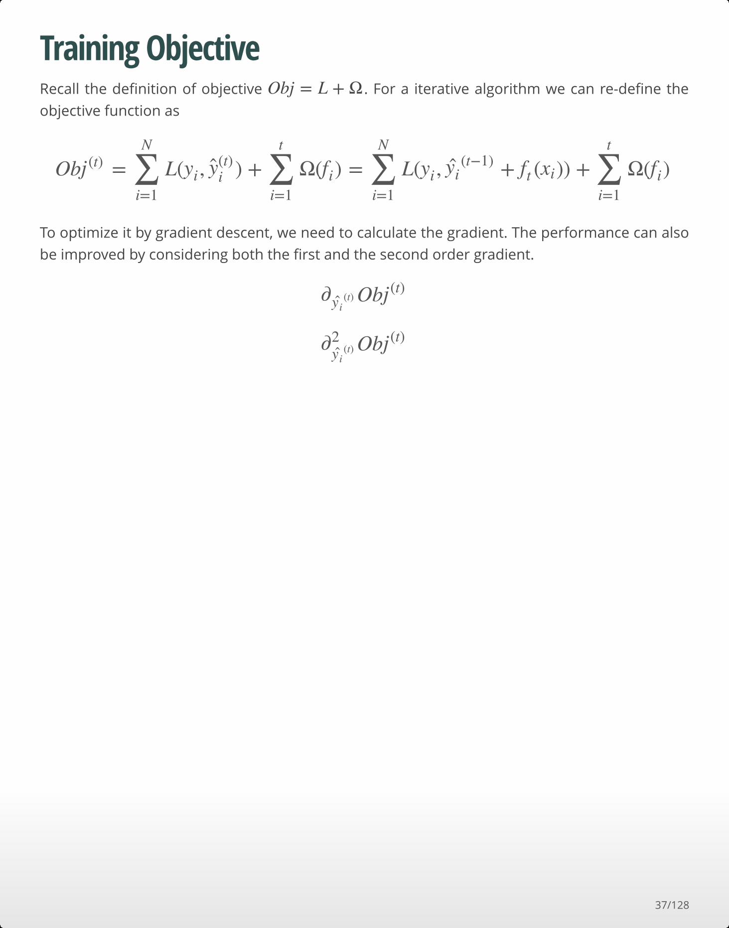
Training ObjectiveRecall the definition of objective . For a iterative algorithm we can re-define the

objective function as

To optimize it by gradient descent, we need to calculate the gradient. The performance can also

be improved by considering both the first and the second order gradient.

Obj = L + Ω

Ob = L( , ) + Ω( ) = L( , + ( )) + Ω( )j (t) ∑i=1

N

yi y(t)i ∑

i=1

t

fi ∑i=1

N

yi yi(t−1) ft xi ∑

i=1

t

fi

Ob∂yi(t) j(t)

Ob∂2yi

(t) j(t)

37/128

Training ObjectiveSince we don't have derivative for every objective function, we calculate the second order taylor

approximation of it

where

Ob ≃ [L( , ) + ( ) + ( )] + Ω( )j(t) ∑i=1

N

yi y(t−1) gift xi12

hif 2t xi ∑

i=1

t

fi

· = l( , )gi ∂ y(t−1) yi y(t−1)

· = l( , )hi ∂2y(t−1) yi y(t−1)

38/128

Training ObjectiveRemove the constant terms, we get

This is the objective at the -th step. Our goal is to find a to optimize it.

Ob = [ ( ) + ( )] + Ω( )j(t) ∑i=1

n

gift xi12

hif 2t xi ft

t ft

39/128

Tree Building AlgorithmThe tree structures in XGBoost leads to the core problem:

how can we find a tree that improves the prediction along the gradient?

40/128

Tree Building AlgorithmEvery decision tree looks like this

Each data point flows to one of the leaves following the direction on each node.

41/128

Tree Building AlgorithmThe core concepts are:

Internal Nodes

Leaves

·

Each internal node split the flow of data points by one of the features.

The condition on the edge specifies what data can flow through.

-

-

·

Data points reach to a leaf will be assigned a weight.

The weight is the prediction.

-

-

42/128

Tree Building AlgorithmTwo key questions for building a decision tree are

1. How to find a good structure?

2. How to assign prediction score?

We want to solve these two problems with the idea of gradient descent.

43/128

Tree Building AlgorithmLet us assume that we already have the solution to question 1.

We can mathematically define a tree as

where is a "directing" function which assign every data point to the -th leaf.

This definition describes the prediction process on a tree as

(x) =ft wq(x)

q(x) q(x)

Assign the data point to a leaf by

Assign the corresponding score on the -th leaf to the data point.

· x q

· wq(x) q(x)

44/128

Tree Building AlgorithmDefine the index set

This set contains the indices of data points that are assigned to the -th leaf.

= {i|q( ) = j}Ij xi

j

45/128

Tree Building AlgorithmThen we rewrite the objective as

Since all the data points on the same leaf share the same prediction, this form sums the

prediction by leaves.

Ob = [ ( ) + ( )] + γT + λj(t) ∑i=1

n

gift xi12

hif 2t xi

12 ∑

j=1

T

w2j

= [( ) + ( + λ) ] + γT∑j=1

T

∑i∈Ij

gi wj12 ∑

i∈Ij

hi w2j

46/128

Tree Building AlgorithmIt is a quadratic problem of , so it is easy to find the best to optimize .

The corresponding value of is

wj wj Obj

= −w∗j

∑i∈Ijgi

+ λ∑i∈Ijhi

Obj

Ob = − + γTj (t) 12 ∑

j=1

T (∑i∈Ijgi)2

+ λ∑i∈Ijhi

47/128

Tree Building AlgorithmThe leaf score

relates to

= −wj

∑i∈Ijgi

+ λ∑i∈Ijhi

The first and second order of the loss function and

The regularization parameter

· g h

· λ

48/128

Tree Building AlgorithmNow we come back to the first question: How to find a good structure?

We can further split it into two sub-questions:

1. How to choose the feature to split?

2. When to stop the split?

49/128

Tree Building AlgorithmIn each split, we want to greedily find the best splitting point that can optimize the objective.

For each feature

1. Sort the numbers

2. Scan the best splitting point.

3. Choose the best feature.

50/128

Tree Building AlgorithmNow we give a definition to "the best split" by the objective.

Everytime we do a split, we are changing a leaf into a internal node.

51/128

Tree Building AlgorithmLet

Recall the best value of objective on the -th leaf is

be the set of indices of data points assigned to this node

and be the sets of indices of data points assigned to two new leaves.

· I

· IL IR

j

Ob = − + γj (t) 12

(∑i∈Ijgi)2

+ λ∑i∈Ijhi

52/128

Tree Building AlgorithmThe gain of the split is

gain = [ + − ] − γ12

(∑i∈ILgi)2

+ λ∑i∈ILhi

(∑i∈IRgi)2

+ λ∑i∈IRhi

(∑i∈I gi)2

+ λ∑i∈I hi

53/128

Tree Building AlgorithmTo build a tree, we find the best splitting point recursively until we reach to the maximum

depth.

Then we prune out the nodes with a negative gain in a bottom-up order.

54/128

Tree Building AlgorithmXGBoost can handle missing values in the data.

For each node, we guide all the data points with a missing value

Finally every node has a "default direction" for missing values.

to the left subnode, and calculate the maximum gain

to the right subnode, and calculate the maximum gain

Choose the direction with a larger gain

·

·

·

55/128

Tree Building AlgorithmTo sum up, the outline of the algorithm is

Iterate for nround times·

Grow the tree to the maximun depth

Prune the tree to delete nodes with negative gain

-

Find the best splitting point

Assign weight to the two new leaves

-

-

-

56/128

Parameters

57/128

Parameter IntroductionXGBoost has plenty of parameters. We can group them into

1. General parameters

2. Booster parameters

3. Task parameters

Number of threads·

Stepsize

Regularization

·

·

Objective

Evaluation metric

·

·

58/128

Parameter IntroductionAfter the introduction of the model, we can understand the parameters provided in XGBoost.

To check the parameter list, one can look into

The documentation of xgb.train.

The documentation in the repository.

·

·

59/128

https://github.com/dmlc/xgboost/blob/master/doc/parameter.md

Parameter IntroductionGeneral parameters:

nthread

booster

·

Number of parallel threads.-

·

gbtree: tree-based model.

gblinear: linear function.

-

-

60/128

Parameter IntroductionParameter for Tree Booster

eta

gamma

·

Step size shrinkage used in update to prevents overfitting.

Range in [0,1], default 0.3

-

-

·

Minimum loss reduction required to make a split.

Range [0, ], default 0

-

- ∞

61/128


max_depth

min_child_weight

max_delta_step

·

Maximum depth of a tree.


-

- ∞·

Minimum sum of instance weight needed in a child.


-

- ∞·

Maximum delta step we allow each tree's weight estimation to be.


-

- ∞

62/128


subsample

colsample_bytree

·

Subsample ratio of the training instance.

Range (0, 1], default 1

-

-

·

Subsample ratio of columns when constructing each tree.

Range (0, 1], default 1

-

-

63/128

Parameter IntroductionParameter for Linear Booster

lambda

alpha

lambda_bias

·

L2 regularization term on weights

default 0

-

-

·

L1 regularization term on weights

default 0

-

-

·

L2 regularization term on bias

default 0

-

-

64/128

Parameter IntroductionObjectives·

"reg:linear": linear regression, default option.

"binary:logistic": logistic regression for binary classification, output probability

"multi:softmax": multiclass classification using the softmax objective, need to specify

num_class

User specified objective

-

-

-

-

65/128

Parameter IntroductionEvaluation Metric·

"rmse"

"logloss"

"error"

"auc"

"merror"

"mlogloss"

User specified evaluation metric

-

-

-

-

-

-

-

66/128

Guide on Parameter TuningIt is nearly impossible to give a set of universal optimal parameters, or a global algorithm

achieving it.

The key points of parameter tuning are

Control Overfitting

Deal with Imbalanced data

Trust the cross validation

·

·

·

67/128

Guide on Parameter TuningThe "Bias-Variance Tradeoff", or the "Accuracy-Simplicity Tradeoff" is the main idea for

controlling overfitting.

For the booster specific parameters, we can group them as

Controlling the model complexity

Robust to noise

·

max_depth, min_child_weight and gamma-

·

subsample, colsample_bytree-

68/128

Guide on Parameter TuningSometimes the data is imbalanced among classes.

Only care about the ranking order

Care about predicting the right probability

·

Balance the positive and negative weights, by scale_pos_weight

Use "auc" as the evaluation metric

-

-

·

Cannot re-balance the dataset

Set parameter max_delta_step to a finite number (say 1) will help convergence

-

-

69/128

Guide on Parameter TuningTo select ideal parameters, use the result from xgb.cv.

Trust the score for the test

Use early.stop.round to detect continuously being worse on test set.

If overfitting observed, reduce stepsize eta and increase nround at the same time.

·

·

·

70/128

Advanced Features

71/128

Advanced FeaturesThere are plenty of highlights in XGBoost:

Customized objective and evaluation metric

Prediction from cross validation

Continue training on existing model

Calculate and plot the variable importance

·

·

·

·

72/128

CustomizationAccording to the algorithm, we can define our own loss function, as long as we can calculate the

first and second order gradient of the loss function.

Define and . We can optimize the loss function if we can calculate

these two values.

grad = l∂yt−1 hess = l∂2yt−1

73/128

CustomizationWe can rewrite logloss for the -th data point as

The is calculated by applying logistic transformation on our prediction .

Then the logloss is

i

L = log( ) + (1 − ) log(1 − )yi pi yi pi

pi yi

L = log + (1 − ) logyi1

1 + e−yiyi

e−yi

1 + e−yi

74/128

CustomizationWe can see that

Next we translate them into the code.

· grad = − = −11+e−yi

yi pi yi

· hess = = (1 − )1+e−yi

(1+e−yi )2 pi pi

75/128

CustomizationThe complete code:

logregobj = function(preds, dtrain) {

labels = getinfo(dtrain, "label")

preds = 1/(1 + exp(-preds))

grad = preds - labels

hess = preds * (1 - preds)

return(list(grad = grad, hess = hess))

}

76/128



# Extract the true label from the second argument






}

77/128





# apply logistic transformation to the output





}

78/128







# Calculate the 1st gradient




}

79/128









# Calculate the 2nd gradient



}

80/128









# Calculate the 2nd gradient


# Return the result


}

81/128

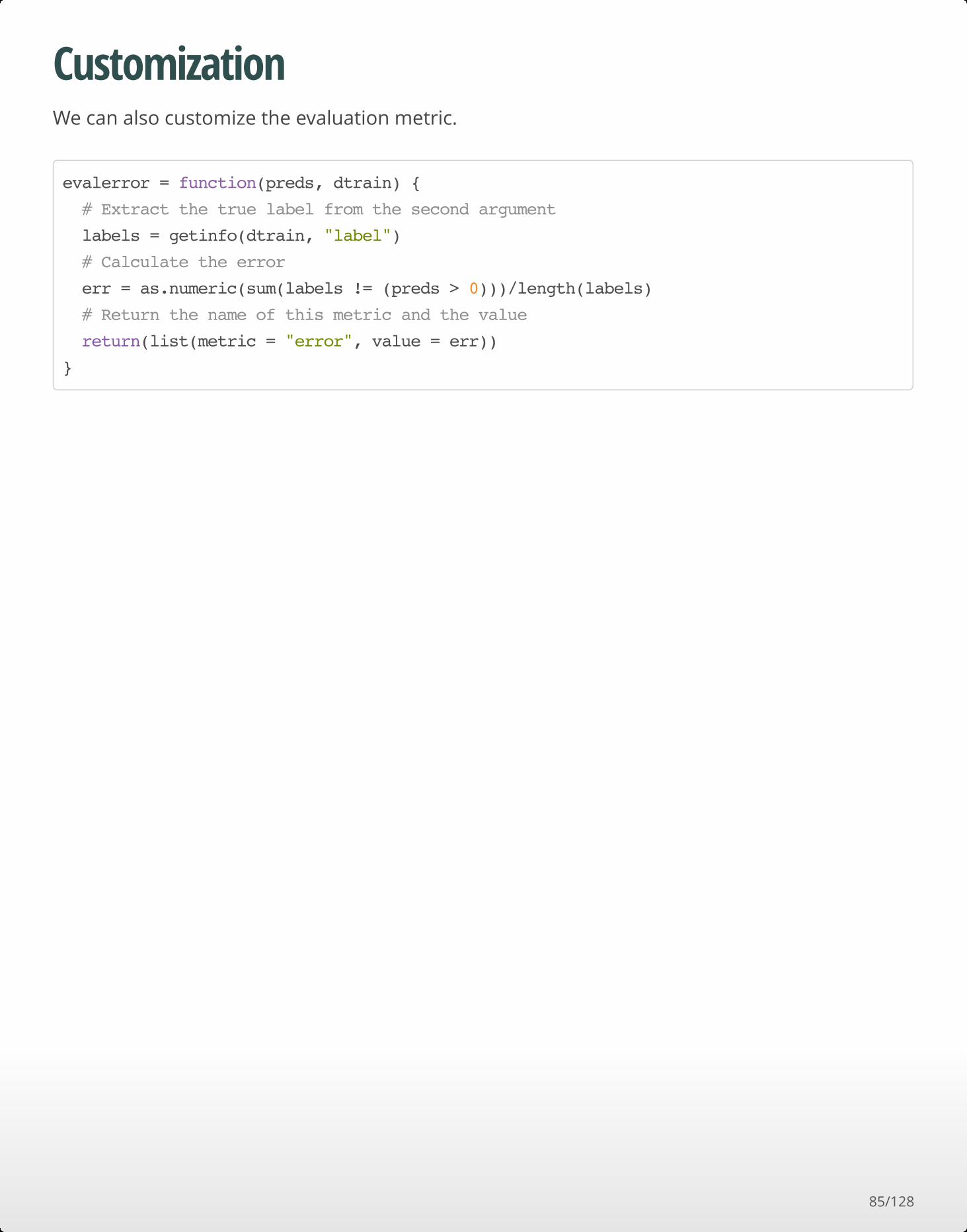
CustomizationWe can also customize the evaluation metric.

evalerror = function(preds, dtrain) {


err = as.numeric(sum(labels != (preds > 0)))/length(labels)

return(list(metric = "error", value = err))

}

82/128







}

83/128





# Calculate the error



}

84/128





# Calculate the error


# Return the name of this metric and the value


}

85/128

CustomizationTo utilize the customized objective and evaluation, we simply pass them to the arguments:

param = list(max.depth=2,eta=1,nthread = 2, silent=1,

objective=logregobj, eval_metric=evalerror)

bst = xgboost(params = param, data = train$data, label = train$label, nround = 2)

## [0] train-error:0.0465223399355136

## [1] train-error:0.0222631659757408

86/128

Prediction in Cross Validation"Stacking" is an ensemble learning technique which takes the prediction from several models. It

is widely used in many scenarios.

One of the main concern is avoid overfitting. The common way is use the prediction value from

cross validation.

XGBoost provides a convenient argument to calculate the prediction during the cross validation.

87/128

Prediction in Cross Validationres = xgb.cv(params = param, data = train$data, label = train$label, nround = 2,

nfold=5, prediction = TRUE)

## [0] train-error:0.046522+0.001347 test-error:0.046522+0.005387


str(res)

## List of 2

## $ dt :Classes 'data.table' and 'data.frame': 2 obs. of 4 variables:

## ..$ train.error.mean: num [1:2] 0.0465 0.0223

## ..$ train.error.std : num [1:2] 0.001347 0.000637

## ..$ test.error.mean : num [1:2] 0.0465 0.0223

## ..$ test.error.std : num [1:2] 0.00539 0.00254

## ..- attr(*, ".internal.selfref")=<externalptr>

## $ pred: num [1:6513] 2.58 -1.07 -1.03 2.59 -3.03 ...

88/128

xgb.DMatrixXGBoost has its own class of input data xgb.DMatrix. One can convert the usual data set into

it by

It is the data structure used by XGBoost algorithm. XGBoost preprocess the input data and

label into an xgb.DMatrix object before feed it to the training algorithm.

If one need to repeat training process on the same big data set, it is good to use the

xgb.DMatrix object to save preprocessing time.

dtrain = xgb.DMatrix(data = train$data, label = train$label)

89/128

xgb.DMatrixAn xgb.DMatrix object contains

1. Preprocessed training data

2. Several features

Missing values

data weight

·

·

90/128

Continue TrainingTrain the model for 5000 rounds is sometimes useful, but we are also taking the risk of

overfitting.

A better strategy is to train the model with fewer rounds and repeat that for many times. This

enable us to observe the outcome after each step.

91/128

Continue Trainingbst = xgboost(params = param, data = dtrain, nround = 1)

## [0] train-error:0.0465223399355136

ptrain = predict(bst, dtrain, outputmargin = TRUE)

setinfo(dtrain, "base_margin", ptrain)

## [1] TRUE

bst = xgboost(params = param, data = dtrain, nround = 1)

## [0] train-error:0.0222631659757408

92/128

Continue Training# Train with only one round


## [0] train-error:0.0222631659757408



## [1] TRUE


## [0] train-error:0.00706279748195916

93/128



## [0] train-error:0.00706279748195916

# margin means the baseline of the prediction



## [1] TRUE


## [0] train-error:0.0152003684937817

94/128



## [0] train-error:0.0152003684937817



# Set the margin information to the xgb.DMatrix object


## [1] TRUE


## [0] train-error:0.00706279748195916

95/128



## [0] train-error:0.00706279748195916



# Set the margin information to the xgb.DMatrix object


## [1] TRUE

# Train based on the previous result


## [0] train-error:0.00122831260555811

96/128

Importance and Tree plottingThe result of XGBoost contains many trees. We can count the number of appearance of each

variable in all the trees, and use this number as the importance score.

bst = xgboost(data = train$data, label = train$label, max.depth = 2, verbose = FALSE,

eta = 1, nthread = 2, nround = 2,objective = "binary:logistic")

xgb.importance(train$dataDimnames[[2]], model = bst)

## Feature Gain Cover Frequence

## 1: 28 0.67615484 0.4978746 0.4

## 2: 55 0.17135352 0.1920543 0.2

## 3: 59 0.12317241 0.1638750 0.2

## 4: 108 0.02931922 0.1461960 0.2

97/128

Importance and Tree plottingWe can also plot the trees in the model by xgb.plot.tree.

xgb.plot.tree(agaricus.train$data@Dimnames[[2]], model = bst)

98/128

Tree plotting

99/128

Early StoppingWhen doing cross validation, it is usual to encounter overfitting at a early stage of iteration.

Sometimes the prediction gets worse consistantly from round 300 while the total number of

iteration is 1000. To stop the cross validation process, one can use the early.stop.round

argument in xgb.cv.

bst = xgb.cv(params = param, data = train$data, label = train$label,

nround = 20, nfold = 5,

maximize = FALSE, early.stop.round = 3)

100/128

Early Stopping## [0] train-error:0.050783+0.011279 test-error:0.055272+0.013879

















## Stopping. Best iteration: 14

101/128

Kaggle Winning Solution

102/128

Kaggle Winning SolutionTo get a higher rank, one need to push the limit of

1. Feature Engineering

2. Parameter Tuning

3. Model Ensemble

The winning solution in the recent Otto Competition is an excellent example.

103/128

https://www.kaggle.com/c/otto-group-product-classification-challenge/forums/t/14335/1st-place-winner-solution-gilberto-titericz-stanislav-semenov

https://www.kaggle.com/c/otto-group-product-classification-challenge

Kaggle Winning SolutionThey used a 3-layer ensemble learning model, including

33 models on top of the original data

XGBoost, neural network and adaboost on 33 predictions from the models and 8 engineered

features

Weighted average of the 3 prediction from the second step

·

·

·

104/128

Kaggle Winning SolutionThe data for this competition is special: the meanings of the featuers are hidden.

For feature engineering, they generated 8 new features:

Distances to nearest neighbours of each classes

Sum of distances of 2 nearest neighbours of each classes

Sum of distances of 4 nearest neighbours of each classes

Distances to nearest neighbours of each classes in TFIDF space

Distances to nearest neighbours of each classed in T-SNE space (3 dimensions)

Clustering features of original dataset

Number of non-zeros elements in each row

X (That feature was used only in NN 2nd level training)

·

·

·

·

·

·

·

·

105/128

Kaggle Winning SolutionThis means a lot of work. However this also implies they need to try a lot of other models,

although some of them turned out to be not helpful in this competition. Their attempts include:

A lot of training algorithms in first level as

Some preprocessing like PCA, ICA and FFT

Feature Selection

Semi-supervised learning

·

Vowpal Wabbit(many configurations)

R glm, glmnet, scikit SVC, SVR, Ridge, SGD, etc...

-

-

·

·

·

106/128

Influencers in Social NetworksLet's learn to use a single XGBoost model to achieve a high rank in an old competition!

The competition we choose is the Influencers in Social Networks competition.

It was a hackathon in 2013, therefore the size of data is small enough so that we can train the

model in seconds.

107/128

https://www.kaggle.com/c/predict-who-is-more-influential-in-a-social-network

Influencers in Social NetworksFirst let's download the data, and load them into R

train = read.csv('train.csv',header = TRUE)

test = read.csv('test.csv',header = TRUE)

y = train[,1]

train = as.matrix(train[,-1])

test = as.matrix(test)

108/128

Influencers in Social NetworksObserve the data:

colnames(train)

## [1] "A_follower_count" "A_following_count" "A_listed_count"

## [4] "A_mentions_received" "A_retweets_received" "A_mentions_sent"

## [7] "A_retweets_sent" "A_posts" "A_network_feature_1"

## [10] "A_network_feature_2" "A_network_feature_3" "B_follower_count"

## [13] "B_following_count" "B_listed_count" "B_mentions_received"

## [16] "B_retweets_received" "B_mentions_sent" "B_retweets_sent"

## [19] "B_posts" "B_network_feature_1" "B_network_feature_2"

## [22] "B_network_feature_3"

109/128

Influencers in Social NetworksObserve the data:

train[1,]

## A_follower_count A_following_count A_listed_count

## 2.280000e+02 3.020000e+02 3.000000e+00

## A_mentions_received A_retweets_received A_mentions_sent

## 5.839794e-01 1.005034e-01 1.005034e-01

## A_retweets_sent A_posts A_network_feature_1

## 1.005034e-01 3.621501e-01 2.000000e+00

## A_network_feature_2 A_network_feature_3 B_follower_count

## 1.665000e+02 1.135500e+04 3.446300e+04

## B_following_count B_listed_count B_mentions_received

## 2.980800e+04 1.689000e+03 1.543050e+01

## B_retweets_received B_mentions_sent B_retweets_sent

## 3.984029e+00 8.204331e+00 3.324230e-01

## B_posts B_network_feature_1 B_network_feature_2

## 6.988815e+00 6.600000e+01 7.553030e+01

## B_network_feature_3

## 1.916894e+03

110/128

Influencers in Social NetworksThe data contains information from two users in a social network service. Our mission is to

determine who is more influencial than the other one.

This type of data gives us some room for feature engineering.

111/128

Influencers in Social NetworksThe first trick is to increase the information in the data.

Every data point can be expressed as <y, A, B>. Actually it indicates <1-y, B, A> as well.

We can simply use extract this part of information from the training set.

new.train = cbind(train[,12:22],train[,1:11])

train = rbind(train,new.train)

y = c(y,1-y)

112/128

Influencers in Social NetworksThe following feature engineering steps are done on both training and test set. Therefore we

combine them together.

x = rbind(train,test)

113/128

Influencers in Social NetworksThe next step could be calculating the ratio between features of A and B seperately:

followers/following

mentions received/sent

retweets received/sent

followers/posts

retweets received/posts

mentions received/posts

·

·

·

·

·

·

114/128

Influencers in Social NetworksConsidering there might be zeroes, we need to smooth the ratio by a constant.

Next we can calculate the ratio with this helper function.

calcRatio = function(dat,i,j,lambda = 1) (dat[,i]+lambda)/(dat[,j]+lambda)

115/128

Influencers in Social NetworksA.follow.ratio = calcRatio(x,1,2)

A.mention.ratio = calcRatio(x,4,6)

A.retweet.ratio = calcRatio(x,5,7)

A.follow.post = calcRatio(x,1,8)

A.mention.post = calcRatio(x,4,8)

A.retweet.post = calcRatio(x,5,8)

B.follow.ratio = calcRatio(x,12,13)

B.mention.ratio = calcRatio(x,15,17)

B.retweet.ratio = calcRatio(x,16,18)

B.follow.post = calcRatio(x,12,19)

B.mention.post = calcRatio(x,15,19)

B.retweet.post = calcRatio(x,16,19)

116/128

Influencers in Social NetworksCombine the features into the data set.

x = cbind(x[,1:11],

A.follow.ratio,A.mention.ratio,A.retweet.ratio,

A.follow.post,A.mention.post,A.retweet.post,

x[,12:22],

B.follow.ratio,B.mention.ratio,B.retweet.ratio,

B.follow.post,B.mention.post,B.retweet.post)

117/128

Influencers in Social NetworksThen we can compare the difference between A and B. Because XGBoost is scale invariant,

therefore minus and division are the essentially same.

AB.diff = x[,1:17]-x[,18:34]

x = cbind(x,AB.diff)

train = x[1:nrow(train),]

test = x[-(1:nrow(train)),]

118/128

Influencers in Social NetworksNow comes to the modeling part. We investigate how far can we can go with a single model.

The parameter tuning step is very important in this step. We can see the performance from

cross validation.

119/128

Influencers in Social NetworksHere's the xgb.cv with default parameters.

set.seed(1024)

cv.res = xgb.cv(data = train, nfold = 3, label = y, nrounds = 100, verbose = FALSE,

objective='binary:logistic', eval_metric = 'auc')

120/128

Influencers in Social NetworksWe can see the trend of AUC on training and test sets.

121/128

Influencers in Social NetworksIt is obvious our model severly overfits. The direct reason is simple: the default value of eta is

0.3, which is too large for this mission.

Recall the parameter tuning guide, we need to decrease eta and inccrease nrounds based on

the result of cross validation.

122/128

Influencers in Social NetworksAfter some trials, we get the following set of parameters:

set.seed(1024)

cv.res = xgb.cv(data = train, nfold = 3, label = y, nrounds = 3000,

objective='binary:logistic', eval_metric = 'auc',

eta = 0.005, gamma = 1,lambda = 3, nthread = 8,

max_depth = 4, min_child_weight = 1, verbose = F,

subsample = 0.8,colsample_bytree = 0.8)

123/128

Influencers in Social NetworksWe can see the trend of AUC on training and test sets.

124/128

Influencers in Social NetworksNext we extract the best number of iterations.

We calculate the AUC minus the standard deviation, and choose the iteration with the largest

value.

bestRound = which.max(as.matrix(cv.res)[,3]-as.matrix(cv.res)[,4])

bestRound

## [1] 2442

cv.res[bestRound,]

## train.auc.mean train.auc.std test.auc.mean test.auc.std

## 1: 0.934967 0.00125 0.876629 0.002073

125/128

Influencers in Social NetworksThen we train the model with the same set of parameters:

set.seed(1024)

bst = xgboost(data = train, label = y, nrounds = 3000,

objective='binary:logistic', eval_metric = 'auc',

eta = 0.005, gamma = 1,lambda = 3, nthread = 8,

max_depth = 4, min_child_weight = 1,

subsample = 0.8,colsample_bytree = 0.8)

preds = predict(bst,test,ntreelimit = bestRound)

126/128

Influencers in Social NetworksFinally we submit our solution

This wins us top 10 on the leaderboard!

result = data.frame(Id = 1:nrow(test),

Choice = preds)

write.csv(result,'submission.csv',quote=FALSE,row.names=FALSE)

127/128

FAQ

128/128

xgboost - saed sayad · the degree of overﬁtting. xgboost provides a convenient function to do...

Documents