xact‘invar · · 2008-05-16xact‘invar ‘ intro invar‘ is ... of the riemann tensor of a...
TRANSCRIPT

xAct‘Invar ‘
Intro
Invar‘ is currently a package for efficient simplification of the algebraic and differential polynomial scalars (usuallyknown as invariants) of the Riemann tensor of a metric−compatible connection. The medium term goal is generalizingInvar‘ to simplify generic polynomial expressions (with free indices) of the Riemann tensor.
Invar‘ requires the tensor computer algebra system xTensor‘ when running on Mathematica. There is a twinversion for Maple, based on the tensor system Canon. It can be downloaded, under the General Public Licence, from
http://metric.iem.csic.es/Martin−Garcia/xAct/
http://www.lncc.br/~portugal/ (Maple version)
For further information, see the articles
The Invar tensor package, J.M. Martín−García, R. Portugal and L.R.U. Manssur, Comp. Phys. Comm. 177, 640(2007)
The Invar tensor package: Differential invariants of Riemann, J.M. Martín−García, D. Yllanes and R. Portugal,Comp. Phys. Comm. (2008)
Subsection 6.3 contains a number of tests designed to check most capabilities of Invar‘ . They all should give zero.
Load the package and configure
Invar‘ requires the free package xTensor‘ to perform the underlying tensor and permutation manipulations. It canbe downloaded from
http://metric.iem.csic.es/Martin−Garcia/xAct/
For a single−user installation under Linux the file xAct_<version>.tar.gz must be unpacked in the directory $Home/.−Mathematica/Applications giving a directory xAct. Then unpack the Invar.tar.gz file inside the xAct directory. Weassume that configuration in the following. See the Readme file for more information, including installation instructionsfor other operating systems.
We first load the Mathematica kernel, and the xTensor‘ package from the default directory
In[1]:= mathRAM = MemoryInUse@D
Out[1]= 3059792
InvarDoc.nb 1
©2003−2004 José M. Martín−García
In[2]:= << xAct‘xTensor‘
------------------------------------------------------------------------------
--
Package xAct‘xCore‘ version 0.5.0, 82008, 5, 16 <CopyRight HCL 2007 -2008, Jose M.
Martin -Garcia, under the General Public License.
------------------------------------------------------------------------------
--
Package ExpressionManipulation‘
CopyRight HCL 1999 -2008, David J. M. Park and Ted Ersek
------------------------------------------------------------------------------
--
Package xAct‘xPerm‘ version 1.0.1, 82008, 5, 16 <CopyRight HCL 2003 -2008, Jose M.
Martin -Garcia, under the General Public License.
Connecting to external linux executable...
Connection established.
------------------------------------------------------------------------------
--
Package xAct‘xTensor‘ version 0.9.5, 82008, 5, 16 <CopyRight HCL 2002 -2008, Jose M.
Martin -Garcia, under the General Public License.
------------------------------------------------------------------------------
--
These packages come with ABSOLUTELY NO WARRANTY; for details typeDisclaimer @D. This is free software, and you are welcome to redistributeit under certain conditions. See the General Public License for details.
------------------------------------------------------------------------------
--
Note: When loading xTensor‘ inside a Windows environment, a black DOS−like window may appear. This is caused by the C link used to speed computations and should not be closed.
In[3]:= xtensorRAM = MemoryInUse@D - mathRAM
Out[3]= 12729104
2 InvarDoc.nb
©2003−2004 José M. Martín−García
Then we read the Invar‘ package.
In[4]:= <<xAct‘Invar‘
------------------------------------------------------------------------------
--
Package xAct‘Invar‘ version 2.0.2, 82008, 3, 5 <CopyRight HCL 2006 -2008, J. M. Martin -Garcia, D.
Yllanes and R. Portugal, under the General Public License.
------------------------------------------------------------------------------
--
These packages come with ABSOLUTELY NO WARRANTY; for details typeDisclaimer @D. This is free software, and you are welcome to redistributeit under certain conditions. See the General Public License for details.
------------------------------------------------------------------------------
--
** DefConstantSymbol: Defining constant symbol sigma.
** DefConstantSymbol: Defining constant symbol dim.
We see that, in Mathematica 5, the MathKernel takes only 2 Mbytes, xTensor‘ takes 9 Mbytes, and Invar‘ takes 41 Mbytes:
In[5]:= invarRAM = MemoryInUse@D - mathRAM - xtensorRAM
Out[5]= 299616
In[6]:= Remove@mathRAM, xtensorRAM, invarRAMD
Note the structure of the ContextPath. There are six contexts: xAct‘Invar‘ , xAct‘xTensor‘ , xAct‘xPerm‘ and xAct‘Ex−pressionManipulation‘ contain the respective reserved words. System‘ contains Mathematica’s reserved words. The current context Global‘ will contain your definitions and right now it is empty.
In[7]:= $ContextPath
Out[7]= 8xAct‘Invar‘, xAct‘xTensor‘, xAct‘xPerm‘,xAct‘xCore‘, xAct‘ExpressionManipulation‘, Global‘, System‘ <
In[8]:= Context@D
Out[8]= Global‘
In[9]:= ?Global‘*
Information::nomatch : No symbol matching Global‘ * found. More¼
à 1. Example sessionThis is a simple example of the use of Invar‘ . The package is very easy to use: all its capabilities can be controlledthrough 10 basic commands. In addition, you will have to setup a basic xTensor‘ session, which we proceed to donow. We need to start by defining the manifold and metric of the Riemann tensor. For information on xTensor‘ seethe file xTensorDoc.nb.
InvarDoc.nb 3
©2003−2004 José M. Martín−García
Define a 4d manifold M:
In[10]:= DefManifold@M, 81, 2, 3, 4<, 8a, b, c, d, e, f, g, h, i, j, k, l, m, n<D
** DefManifold: Defining manifold M.
** DefVBundle: Defining vbundle TangentM.
Define a metric with negative determinant, with associated Levi−Civita connection CD:
In[11]:= DefMetric@-1, metric@-a, -bD, CD, 8";", "õ"<, CurvatureRelations ® FalseD
** DefTensor: Defining symmetric metric tensor metric @-a, -bD.** DefTensor: Defining antisymmetric tensor epsilonmetric @a, b, c, d D.** DefCovD: Defining covariant derivative CD @-aD.** DefTensor: Defining vanishing torsion tensor TorsionCD @a, -b, -cD.** DefTensor: Defining symmetric Christoffel tensor ChristoffelCD @a, -b, -cD.** DefTensor: Defining Riemann tensor RiemannCD @-a, -b, -c, -dD.** DefTensor: Defining symmetric Ricci tensor RicciCD @-a, -bD.** DefTensor: Defining Ricci scalar RicciScalarCD @D.** DefTensor: Defining symmetric Einstein tensor EinsteinCD @-a, -bD.** DefTensor: Defining Weyl tensor WeylCD @-a, -b, -c, -dD.
Rules 81, 2, 3, 4, 5, 6, 7, 8 < have been declared as DownValues for WeylCD.
** DefTensor: Defining symmetric TFRicci tensor TFRicciCD @-a, -bD.Rules 81, 2 < have been declared as DownValues for TFRicciCD.
** DefCovD: Computing RiemannToWeylRules for dim 4
** DefCovD: Computing RicciToTFRicci for dim 4
** DefCovD: Computing RicciToEinsteinRules for dim 4
We included the option CurvatureRelations −> False so contractions of Riemanns will not be converted into Riccis. A number of tensors have been automatically defined. In particular there are the three curvature tensor fields
In[12]:= RiemannCD@-a, -b, -c, -dD
Out[12]= R@õDabcd
In[13]:= RicciCD@-a, -bD
Out[13]= R@õDab
In[14]:= RicciScalarCD@D
Out[14]= R@õD
4 InvarDoc.nb
©2003−2004 José M. Martín−García
and their traceless counterparts:
In[15]:= WeylCD@-a, -b, -c, -dD
Out[15]= W@õDabcd
In[16]:= TFRicciCD@-a, -bD
Out[16]= S@õDab
with their expected trace properties:
In[17]:= WeylCD@a, -b, -c, -aD
Out[17]= 0
In[18]:= TFRicciCD@-a, aD
Out[18]= 0
The Riemann and Ricci tensors are not automatically replaced when they have contracted indices. Use ContractCurvature to do that:
In[19]:= RiemannCD@a, -b, -c, -aD
Out[19]= R@õD bcaa
In[20]:= ContractCurvature@%D
Out[20]= -R@õDbc
In[21]:= RicciCD@-b, bD
Out[21]= R@õDbb
In[22]:= ContractCurvature@%D
Out[22]= R@õD
We can change the output form of the tensors (note the use of Mathematica downvalues ^= )
In[23]:= PrintAs@metricD ^= "g";PrintAs@epsilonmetricD ^= "Ε";PrintAs@RiemannCDD ^= "R";PrintAs@RicciCDD ^= "R";PrintAs@RicciScalarCDD ^= "R";PrintAs@WeylCDD ^= "W";PrintAs@TFRicciCDD ^= "S";
So much for xTensor‘ . You will not need many more xTensor‘ functions to work with Invar‘ , but you will beable to do it more efficiently if you read the specific documentation for that package. Now we can start using thecommands added by the package Invar‘:
InvarDoc.nb 5
©2003−2004 José M. Martín−García
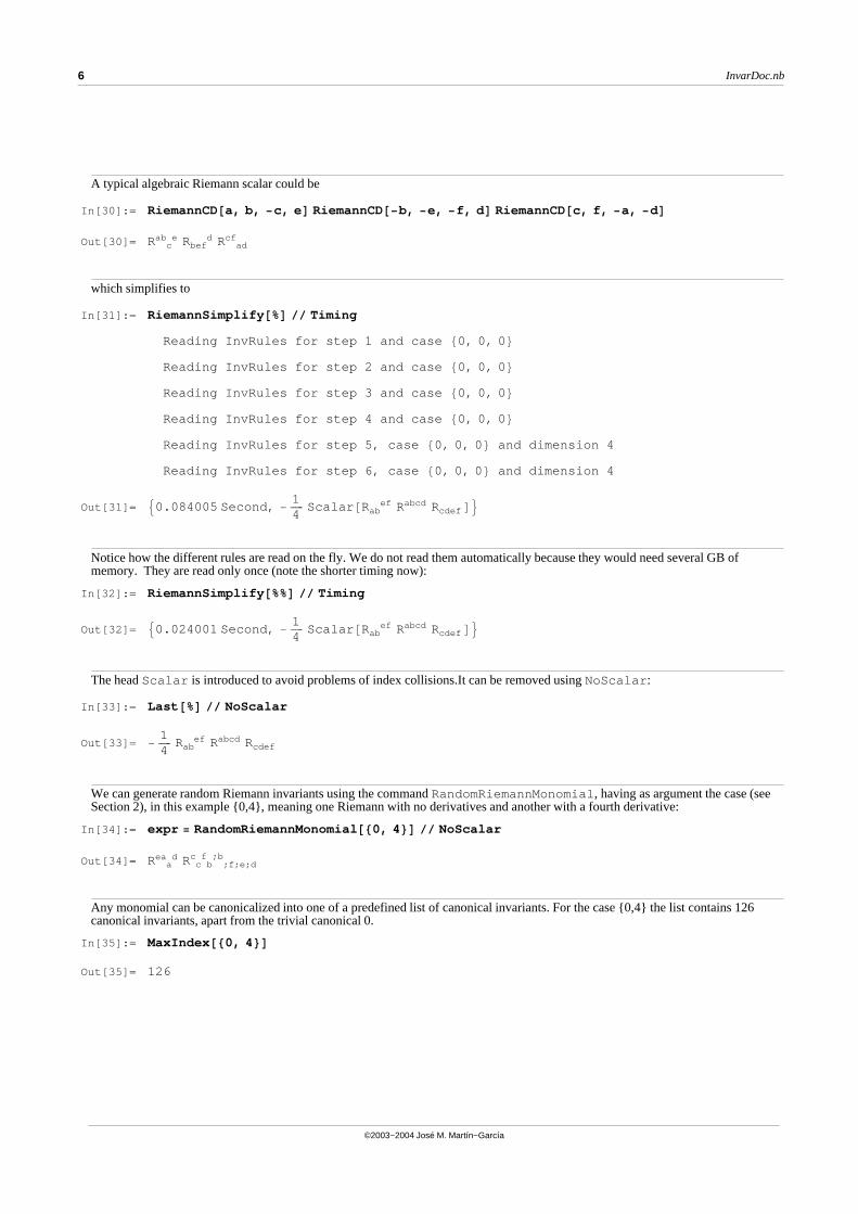
A typical algebraic Riemann scalar could be
In[30]:= RiemannCD@a, b, -c, eD RiemannCD@-b, -e, -f, dD RiemannCD@c, f, -a, -dD
Out[30]= R cab e Rbef
d R adcf
which simplifies to
In[31]:= RiemannSimplify@%D �� Timing
Reading InvRules for step 1 and case 80, 0, 0 <Reading InvRules for step 2 and case 80, 0, 0 <Reading InvRules for step 3 and case 80, 0, 0 <Reading InvRules for step 4 and case 80, 0, 0 <Reading InvRules for step 5, case 80, 0, 0 < and dimension 4
Reading InvRules for step 6, case 80, 0, 0 < and dimension 4
Out[31]= 90.084005 Second, -1�����4
Scalar @Rabef Rabcd Rcdef D=
Notice how the different rules are read on the fly. We do not read them automatically because they would need several GB of memory. They are read only once (note the shorter timing now):
In[32]:= RiemannSimplify@%%D �� Timing
Out[32]= 90.024001 Second, -1�����4
Scalar @Rabef Rabcd Rcdef D=
The head Scalar is introduced to avoid problems of index collisions.It can be removed using NoScalar :
In[33]:= Last@%D �� NoScalar
Out[33]= -1�����4
Rabef Rabcd Rcdef
We can generate random Riemann invariants using the command RandomRiemannMonomial , having as argument the case (see Section 2), in this example {0,4}, meaning one Riemann with no derivatives and another with a fourth derivative:
In[34]:= expr = RandomRiemannMonomial@80, 4<D �� NoScalar
Out[34]= R aea d R c b ;f;e;d
c f ;b
Any monomial can be canonicalized into one of a predefined list of canonical invariants. For the case {0,4} the list contains 126 canonical invariants, apart from the trivial canonical 0.
In[35]:= MaxIndex@80, 4<D
Out[35]= 126
6 InvarDoc.nb
©2003−2004 José M. Martín−García
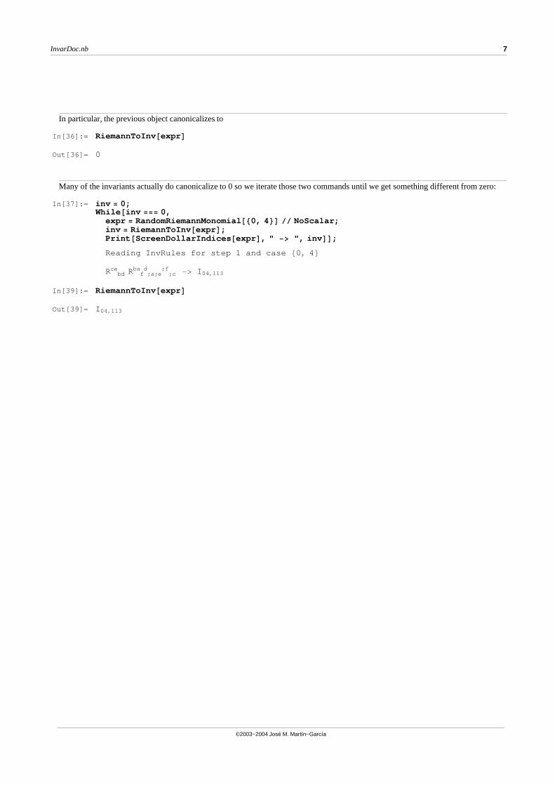
In particular, the previous object canonicalizes to
In[36]:= RiemannToInv@exprD
Out[36]= 0
Many of the invariants actually do canonicalize to 0 so we iterate those two commands until we get something different from zero:
In[37]:= inv = 0;While@inv === 0,expr = RandomRiemannMonomial@80, 4<D �� NoScalar;inv = RiemannToInv@exprD;Print@ScreenDollarIndices@exprD, " -> ", invDD;
Reading InvRules for step 1 and case 80, 4 <
R bdce R f ;a;e ;c
ba d ;f-> I 04,113
In[39]:= RiemannToInv@exprD
Out[39]= I 04,113
InvarDoc.nb 7
©2003−2004 José M. Martín−García
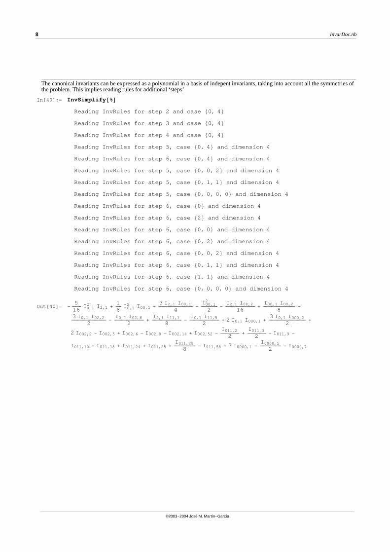
The canonical invariants can be expressed as a polynomial in a basis of indepent invariants, taking into account all the symmetries of the problem. This implies reading rules for additional ‘steps’
In[40]:= InvSimplify@%D
Reading InvRules for step 2 and case 80, 4 <Reading InvRules for step 3 and case 80, 4 <Reading InvRules for step 4 and case 80, 4 <Reading InvRules for step 5, case 80, 4 < and dimension 4
Reading InvRules for step 6, case 80, 4 < and dimension 4
Reading InvRules for step 5, case 80, 0, 2 < and dimension 4
Reading InvRules for step 5, case 80, 1, 1 < and dimension 4
Reading InvRules for step 5, case 80, 0, 0, 0 < and dimension 4
Reading InvRules for step 6, case 80< and dimension 4
Reading InvRules for step 6, case 82< and dimension 4
Reading InvRules for step 6, case 80, 0 < and dimension 4
Reading InvRules for step 6, case 80, 2 < and dimension 4
Reading InvRules for step 6, case 80, 0, 2 < and dimension 4
Reading InvRules for step 6, case 80, 1, 1 < and dimension 4
Reading InvRules for step 6, case 81, 1 < and dimension 4
Reading InvRules for step 6, case 80, 0, 0, 0 < and dimension 4
Out[40]= -5
��������16
I 0,12 I 2,1 +
1�����8
I 0,12 I 00,1 +
3 I 2,1 I 00,1�����������������������������
4-
I 00,12
��������������2
-I 2,1 I 00,2�������������������������
16+
I 00,1 I 00,2���������������������������
8+
3 I 0,1 I 02,2�����������������������������
2-
I 0,1 I 02,6�������������������������
2+
I 0,1 I 11,1�������������������������
8-
I 0,1 I 11,5�������������������������
2+ 2 I 0,1 I 000,1 +
3 I 0,1 I 000,2�������������������������������
2+
2 I 002,2 - I 002,5 + I 002,6 - I 002,8 - I 002,14 + I 002,52 -I 011,2����������������
2+
I 011,3����������������
2- I 011,9 -
I 011,10 + I 011,18 + I 011,24 + I 011,25 +I 011,28������������������
8- I 011,58 + 3 I 0000,1 -
I 0000,5������������������
2- I 0000,7
8 InvarDoc.nb
©2003−2004 José M. Martín−García
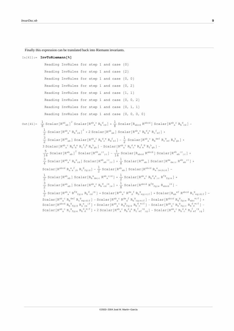
Finally this expression can be translated back into Riemann invariants.
In[41]:= InvToRiemann@%D
Reading InvRules for step 1 and case 80<Reading InvRules for step 1 and case 82<Reading InvRules for step 1 and case 80, 0 <Reading InvRules for step 1 and case 80, 2 <Reading InvRules for step 1 and case 81, 1 <Reading InvRules for step 1 and case 80, 0, 2 <Reading InvRules for step 1 and case 80, 1, 1 <Reading InvRules for step 1 and case 80, 0, 0, 0 <
Out[41]=1�����8
Scalar @R abab D2
Scalar @R aab c Rb cd
d D +1�����8
Scalar @Rabcd Rabcd D Scalar @R aab c Rb cd
d D -
1�����2
Scalar @R aab c Rb cd
d D2+ 2 Scalar @R ab
ab D Scalar @R aab c Rb d
d e Rc eff D +
3�����2
Scalar @R abab D Scalar @R a
ab c Rb cd e Rd ef
f D -1�����2
Scalar @R aab c Rb
def Rc efg Rd gh
h D +
3 Scalar @R aab c Rb d
d e Rc ff g Re gh
h D - Scalar @R aab c Rb c
d e Rd ef g Rf gh
h D -
5��������16
Scalar @R abab D2
Scalar @R ab ;cab ;c D -
1��������16
Scalar @Rabcd Rabcd D Scalar @R ab ;cab ;c D +
3�����4
Scalar @R aab c Rb cd
d D Scalar @R ab ;cab ;c D +
1�����8
Scalar @R abab D Scalar @R de;c
de R abab ;c D +
Scalar @Rabcd Ra e ;be f Rc fg;d
g D -1�����2
Scalar @R abab D Scalar @Rabcd Ra ce;b;d
e D -
1�����2
Scalar @R abab D Scalar @Rb de;c
e R aab c;d D +
1�����2
Scalar @R aab c Rb d ;c
d e R fg;efg D +
3�����2
Scalar @R abab D Scalar @R a
ab c Rb cd ;ed ;e D +
1�����8
Scalar @Rabcd R fg;efg Rabcd
;e D -
1�����2
Scalar @R aab c R fg;e
fg Rb cdd ;e D + Scalar @R a
ab c R dde f Rb eg;c;f
g D + Scalar @Rabef Rabcd Rc eg;d;f
g D -
Scalar @R aab c Rb
def Rc eg;d;fg D - Scalar @R a
ab c R dde f Rb cg;e;f
g D - Scalar @Rabcd Rd fg;eg Rabc
e;f D +
Scalar @Rabcd Rb fg;dg Ra ce
e ;f D + Scalar @R aab c Rd fg;e
g Rb cd e;f D - Scalar @R a
ab c Re fg;cg Rb d
d e;f D -
Scalar @R aab c Rc fg;e
g Rb dd e;f D + 2 Scalar @R a
ab c Rb dd e Rc ef ;g
f ;g D - Scalar @R aab c Rb c
d e Rd ef ;gf ;g D
InvarDoc.nb 9
©2003−2004 José M. Martín−García
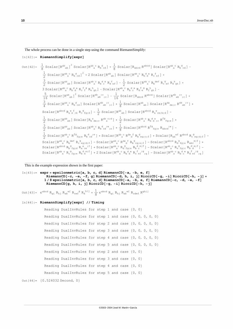
The whole process can be done in a single step using the command RiemannSimplify:
In[42]:= RiemannSimplify@exprD
Out[42]=1�����8
Scalar @R abab D2
Scalar @R aab c Rb cd
d D +1�����8
Scalar @Rabcd Rabcd D Scalar @R aab c Rb cd
d D -
1�����2
Scalar @R aab c Rb cd
d D2+ 2 Scalar @R ab
ab D Scalar @R aab c Rb d
d e Rc eff D +
3�����2
Scalar @R abab D Scalar @R a
ab c Rb cd e Rd ef
f D -1�����2
Scalar @R aab c Rb
def Rc efg Rd gh
h D +
3 Scalar @R aab c Rb d
d e Rc ff g Re gh
h D - Scalar @R aab c Rb c
d e Rd ef g Rf gh
h D -
5��������16
Scalar @R abab D2
Scalar @R ab ;cab ;c D -
1��������16
Scalar @Rabcd Rabcd D Scalar @R ab ;cab ;c D +
3�����4
Scalar @R aab c Rb cd
d D Scalar @R ab ;cab ;c D +
1�����8
Scalar @R abab D Scalar @R de;c
de R abab ;c D +
Scalar @Rabcd Ra e ;be f Rc fg;d
g D -1�����2
Scalar @R abab D Scalar @Rabcd Ra ce;b;d
e D -
1�����2
Scalar @R abab D Scalar @Rb de;c
e R aab c;d D +
1�����2
Scalar @R aab c Rb d ;c
d e R fg;efg D +
3�����2
Scalar @R abab D Scalar @R a
ab c Rb cd ;ed ;e D +
1�����8
Scalar @Rabcd R fg;efg Rabcd
;e D -
1�����2
Scalar @R aab c R fg;e
fg Rb cdd ;e D + Scalar @R a
ab c R dde f Rb eg;c;f
g D + Scalar @Rabef Rabcd Rc eg;d;f
g D -
Scalar @R aab c Rb
def Rc eg;d;fg D - Scalar @R a
ab c R dde f Rb cg;e;f
g D - Scalar @Rabcd Rd fg;eg Rabc
e;f D +
Scalar @Rabcd Rb fg;dg Ra ce
e ;f D + Scalar @R aab c Rd fg;e
g Rb cd e;f D - Scalar @R a
ab c Re fg;cg Rb d
d e;f D -
Scalar @R aab c Rc fg;e
g Rb dd e;f D + 2 Scalar @R a
ab c Rb dd e Rc ef ;g
f ;g D - Scalar @R aab c Rb c
d e Rd ef ;gf ;g D
This is the example expression shown in the first paper:
In[43]:= expr = epsilonmetric@a, b, c, dD RiemannCD@-a, -b, e, fD
RiemannCD@-c, -e, -f, gD RiemannCD@-d, h, i, jD RicciCD@-g, -iD RicciCD@-h, -jD +
1�8 epsilonmetric@a, b, c, dD RiemannCD@-a, -b, e, fD RiemannCD@-c, -d, -e, -fD
RiemannCD@g, h, i, jD RicciCD@-g, -iD RicciCD@-h, -jD
Out[43]= Εabcd Rgi Rhj Rab
ef Rcefg Rd
hij+
1�����8
Εabcd Rgi Rhj Rab
ef Rcdef Rghij
In[44]:= RiemannSimplify@exprD �� Timing
Reading DualInvRules for step 1 and case 80, 0 <Reading DualInvRules for step 1 and case 80, 0, 0, 0, 0 <Reading DualInvRules for step 2 and case 80, 0, 0, 0, 0 <Reading DualInvRules for step 3 and case 80, 0, 0, 0, 0 <Reading DualInvRules for step 4 and case 80, 0, 0, 0, 0 <Reading DualInvRules for step 5 and case 80, 0, 0, 0, 0 <Reading DualInvRules for step 2 and case 80, 0 <Reading DualInvRules for step 3 and case 80, 0 <Reading DualInvRules for step 4 and case 80, 0 <Reading DualInvRules for step 5 and case 80, 0 <
Out[44]= 80.524032 Second, 0 <
10 InvarDoc.nb
©2003−2004 José M. Martín−García
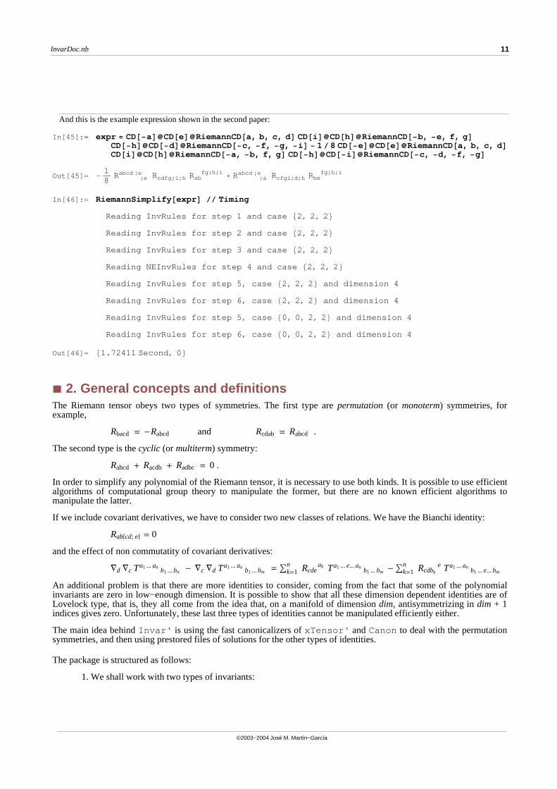
And this is the example expression shown in the second paper:
In[45]:= expr = CD@-aD�CD@eD�RiemannCD@a, b, c, dD CD@iD�CD@hD�RiemannCD@-b, -e, f, gD
CD@-hD�CD@-dD�RiemannCD@-c, -f, -g, -iD - 1�8 CD@-eD�CD@eD�RiemannCD@a, b, c, dD
CD@iD�CD@hD�RiemannCD@-a, -b, f, gD CD@-hD�CD@-iD�RiemannCD@-c, -d, -f, -gD
Out[45]= -1�����8
R ;eabcd ;e Rcdfg;i;h Rab
fg;h;i+ R ;a
abcd ;e Rcfgi;d;h Rbefg;h;i
In[46]:= RiemannSimplify@exprD �� Timing
Reading InvRules for step 1 and case 82, 2, 2 <Reading InvRules for step 2 and case 82, 2, 2 <Reading InvRules for step 3 and case 82, 2, 2 <Reading NEInvRules for step 4 and case 82, 2, 2 <Reading InvRules for step 5, case 82, 2, 2 < and dimension 4
Reading InvRules for step 6, case 82, 2, 2 < and dimension 4
Reading InvRules for step 5, case 80, 0, 2, 2 < and dimension 4
Reading InvRules for step 6, case 80, 0, 2, 2 < and dimension 4
Out[46]= 81.72411 Second, 0 <
à 2. General concepts and definitionsThe Riemann tensor obeys two types of symmetries. The first type are permutation (or monoterm) symmetries, forexample,
Rbacd = -Rabcd and Rcdab = Rabcd .
The second type is the cyclic (or multiterm) symmetry:
Rabcd + Racdb + Radbc = 0 .
In order to simplify any polynomial of the Riemann tensor, it is necessary to use both kinds. It is possible to use efficientalgorithms of computational group theory to manipulate the former, but there are no known efficient algorithms tomanipulate the latter.
If we include covariant derivatives, we have to consider two new classes of relations. We have the Bianchi identity:
Rab@cd; eD = 0
and the effect of non commutatity of covariant derivatives:
Ñd Ñc Ta1 ...anb1 ... bn - Ñc Ñd Ta1 ...an
b1 ... bm = Úk=1n
Rcdeak Ta1 ... e... an
b1 ... bm -Úk=1n
Rcdbk
e Ta1 ... an
b1 ... e... bm
An additional problem is that there are more identities to consider, coming from the fact that some of the polynomialinvariants are zero in low−enough dimension. It is possible to show that all these dimension dependent identities are ofLovelock type, that is, they all come from the idea that, on a manifold of dimension dim, antisymmetrizing in dim + 1indices gives zero. Unfortunately, these last three types of identities cannot be manipulated efficiently either.
The main idea behind Invar‘ is using the fast canonicalizers of xTensor‘ and Canon to deal with the permutationsymmetries, and then using prestored files of solutions for the other types of identities.
The package is structured as follows:
1. We shall work with two types of invariants:
InvarDoc.nb 11
©2003−2004 José M. Martín−García
1. We shall work with two types of invariants:
− (non−dual) invariants: fully contracted products of n Riemann tensors (where n will be called thedegree of the invariant), possibly including covariant derivatives .
− dual invariants: fully contracted products of n Riemann tensors with or without derivatives and oneepsilon tensor (n is again called the degree of the dual invariant). There is no need to work with more than one epsilon,because products of two epsilons can be converted into delta tensors.
We shall separate the set of all monomial invariants of degree n in subsets R8Λ1 , ... ,Λn < , where Λi is the differentiationorder of the i−th Riemann tensor, assuming the tensors have sorted such that Λi £ Λi+ . An n−tuple {Λ1 , ..., Λn} will bereferred to as a case, with the corresponding invariants having N = 4n +Úi=1
n Λi indices and order L = 2n + Úi=1n
Λi . L isthe number of derivatives of the metric, not to be confused with the total number of derivatives of the Riemann tensors(the sum of the Λi ’s). Both N and L are always even numbers because we only consider scalar expressions. For example,an invariant of the case {0,1,3}, hence with N = 16 indices and order L = 10, is
Rabcd Ñe Recfg Ñ
a Ñ f Ñh Rbdh
g .
2. We shall distinguish six steps or levels of simplification:
1.− Canonicalization with respect to permutation symmetries.
2.− Canonicalization with respect to the cyclic symmetry.
3.− Canonicalization with respect to the Bianchi symmetry.
4.− Canonicalization with respect to commutation of derivatives.
5.− Use of all possible dimensionally−dependent identities.
6.− Conversion of invariants into products of two dual invariants (metric−signature dependent).
3. Each Riemann monomial can be represented in one of three forms (examples will be given below):
− As an explicit tensor expression.
− As a permutation of the indices in canonical order.
− As an expression RInv[metric][case, index] or DualRInv[metric][case, index]which represents the equivalent canonical monomial after canonicalization with respect to the permutation symmetries.The integer index identifies each particular invariant in the list of invariants, sorted according to some predefinedordering.
4. Commands are given to change among those three representations, and to simplify the invariants up to someparticular level. They are all listed below. Their mutual structure is schematically given by
In[47]:= << Graphics‘Arrow‘
12 InvarDoc.nb
©2003−2004 José M. Martín−García
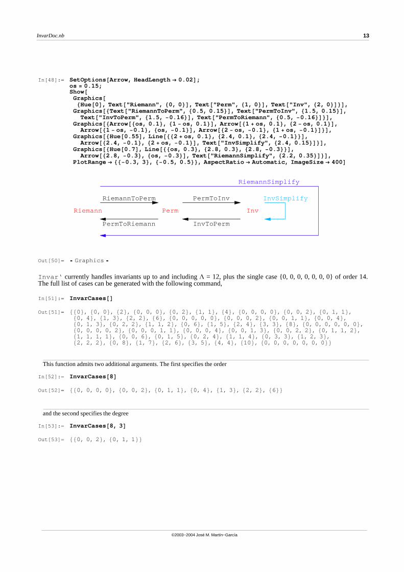
In[48]:= SetOptions@Arrow, HeadLength ® 0.02D;os = 0.15;Show@Graphics@8Hue@0D, Text@"Riemann", 80, 0<D, Text@"Perm", 81, 0<D, Text@"Inv", 82, 0<D<D,Graphics@8Text@"RiemannToPerm", 80.5, 0.15<D, Text@"PermToInv", 81.5, 0.15<D,Text@"InvToPerm", 81.5, -0.16<D, Text@"PermToRiemann", 80.5, -0.16<D<D,
Graphics@8Arrow@8os, 0.1<, 81 - os, 0.1<D, Arrow@81 + os, 0.1<, 82 - os, 0.1<D,Arrow@81 - os, -0.1<, 8os, -0.1<D, Arrow@82 - os, -0.1<, 81 + os, -0.1<D<D,
Graphics@[email protected], Line@882 + os, 0.1<, 82.4, 0.1<, 82.4, -0.1<<D,[email protected], -0.1<, 82 + os, -0.1<D, Text@"InvSimplify", 82.4, 0.15<D<D,
Graphics@[email protected], Line@88os, 0.3<, 82.8, 0.3<, 82.8, -0.3<<D,[email protected], -0.3<, 8os, -0.3<D, Text@"RiemannSimplify", 82.2, 0.35<D<D,
PlotRange ® 88-0.3, 3<, 8-0.5, 0.5<<, AspectRatio ® Automatic, ImageSize ® 400D
Riemann Perm Inv
RiemannToPerm PermToInv
InvToPermPermToRiemann
InvSimplify
RiemannSimplify
Out[50]= � Graphics �
Invar‘ currently handles invariants up to and including L = 12, plus the single case {0, 0, 0, 0, 0, 0, 0} of order 14.The full list of cases can be generated with the following command,
In[51]:= InvarCases@D
Out[51]= 880<, 80, 0 <, 82<, 80, 0, 0 <, 80, 2 <, 81, 1 <, 84<, 80, 0, 0, 0 <, 80, 0, 2 <, 80, 1, 1 <,80, 4 <, 81, 3 <, 82, 2 <, 86<, 80, 0, 0, 0, 0 <, 80, 0, 0, 2 <, 80, 0, 1, 1 <, 80, 0, 4 <,80, 1, 3 <, 80, 2, 2 <, 81, 1, 2 <, 80, 6 <, 81, 5 <, 82, 4 <, 83, 3 <, 88<, 80, 0, 0, 0, 0, 0 <,80, 0, 0, 0, 2 <, 80, 0, 0, 1, 1 <, 80, 0, 0, 4 <, 80, 0, 1, 3 <, 80, 0, 2, 2 <, 80, 1, 1, 2 <,81, 1, 1, 1 <, 80, 0, 6 <, 80, 1, 5 <, 80, 2, 4 <, 81, 1, 4 <, 80, 3, 3 <, 81, 2, 3 <,82, 2, 2 <, 80, 8 <, 81, 7 <, 82, 6 <, 83, 5 <, 84, 4 <, 810<, 80, 0, 0, 0, 0, 0, 0 <<
This function admits two additional arguments. The first specifies the order
In[52]:= InvarCases@8D
Out[52]= 880, 0, 0, 0 <, 80, 0, 2 <, 80, 1, 1 <, 80, 4 <, 81, 3 <, 82, 2 <, 86<<
and the second specifies the degree
In[53]:= InvarCases@8, 3D
Out[53]= 880, 0, 2 <, 80, 1, 1 <<
InvarDoc.nb 13
©2003−2004 José M. Martín−García
à 3. Canonical invariants
RInv Non−dual invariant DualRInv Dual invariantRInvs List of all non−dual invariants after a given stepDualRInvs List of all dual invariants after a given stepMaxIndex Maximum value of the index for the list of non−dual invariant after a given stepMaxDualIndex Maximum value of the index for the list of dual invariants after a given stepRInvRules List of all independent invariants for a given step and caseRemoveRInvRules Remove rules for invariants of a given step and case
Canonical invariants
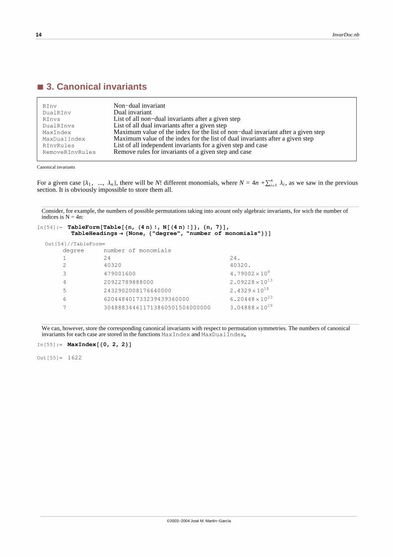
For a given case 8Λ1 , ..., Λn<, there will be N! different monomials, where N = 4n +Úi=1n Λi , as we saw in the previous
section. It is obviously impossible to store them all.
Consider, for example, the numbers of possible permutations taking into acount only algebraic invariants, for wich the number of indices is N = 4n:
In[54]:= TableForm@Table@8n, H4 nL!, N@H4 nL!D<, 8n, 7<D,TableHeadings ® 8None, 8"degree", "number of monomials"<<D
Out[54]//TableForm=degree number of monomials1 24 24.2 40320 40320.
3 479001600 4.79002 ´ 108
4 20922789888000 2.09228 ´ 1013
5 2432902008176640000 2.4329 ´ 1018
6 620448401733239439360000 6.20448 ´ 1023
7 304888344611713860501504000000 3.04888 ´ 1029
We can, however, store the corresponding canonical invariants with respect to permutation symmetries. The numbers of canonical invariants for each case are stored in the functions MaxIndex and MaxDualIndex ,
In[55]:= MaxIndex@80, 2, 2<D
Out[55]= 1622
14 InvarDoc.nb
©2003−2004 José M. Martín−García
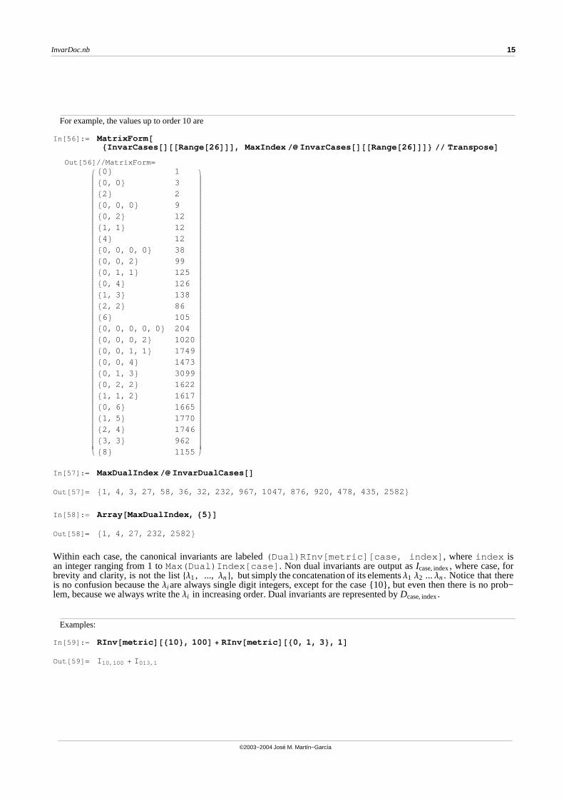
For example, the values up to order 10 are
In[56]:= MatrixForm@8InvarCases@D@@Range@26DDD, MaxIndex �� InvarCases@D@@Range@26DDD< �� TransposeD
Out[56]//MatrixForm=
i
k
jjjjjjjjjjjjjjjjjjjjjjjjjjjjjjjjjjjjjjjjjjjjjjjjjjjjjjjjjjjjjjjjjjjjjjjjjjjjjjjjjjjjjjjjjjjjjjjjjjjjjjjjjjjjjjjjjjjjjjjjjjjjj
80< 180, 0 < 382< 280, 0, 0 < 980, 2 < 1281, 1 < 1284< 1280, 0, 0, 0 < 3880, 0, 2 < 9980, 1, 1 < 12580, 4 < 12681, 3 < 13882, 2 < 8686< 10580, 0, 0, 0, 0 < 20480, 0, 0, 2 < 102080, 0, 1, 1 < 174980, 0, 4 < 147380, 1, 3 < 309980, 2, 2 < 162281, 1, 2 < 161780, 6 < 166581, 5 < 177082, 4 < 174683, 3 < 96288< 1155
y
{
zzzzzzzzzzzzzzzzzzzzzzzzzzzzzzzzzzzzzzzzzzzzzzzzzzzzzzzzzzzzzzzzzzzzzzzzzzzzzzzzzzzzzzzzzzzzzzzzzzzzzzzzzzzzzzzzzzzzzzzzzzzzz
In[57]:= MaxDualIndex �� InvarDualCases@D
Out[57]= 81, 4, 3, 27, 58, 36, 32, 232, 967, 1047, 876, 920, 478, 435, 2582 <
In[58]:= Array@MaxDualIndex, 85<D
Out[58]= 81, 4, 27, 232, 2582 <
Within each case, the canonical invariants are labeled (Dual)RInv[metric][case, index] , where index isan integer ranging from 1 to Max(Dual)Index[case] . Non dual invariants are output as Icase, index, where case, forbrevity and clarity, is not the list 8Λ1 , ..., Λn<, but simply the concatenation of its elementsΛ1 Λ2 ... Λn . Notice that thereis no confusion because the Λi are always single digit integers, except for the case {10}, but even then there is no prob−lem, because we always write the Λi in increasing order. Dual invariants are represented by Dcase, index.
Examples:
In[59]:= RInv@metricD@810<, 100D + RInv@metricD@80, 1, 3<, 1D
Out[59]= I 10,100 + I 013,1
InvarDoc.nb 15
©2003−2004 José M. Martín−García
In[60]:= RInv@metricD@80, 1, 2<, 12D - DualRInv@metricD@80, 0, 0<, 1D
Out[60]= -D000,1 + I 012,12
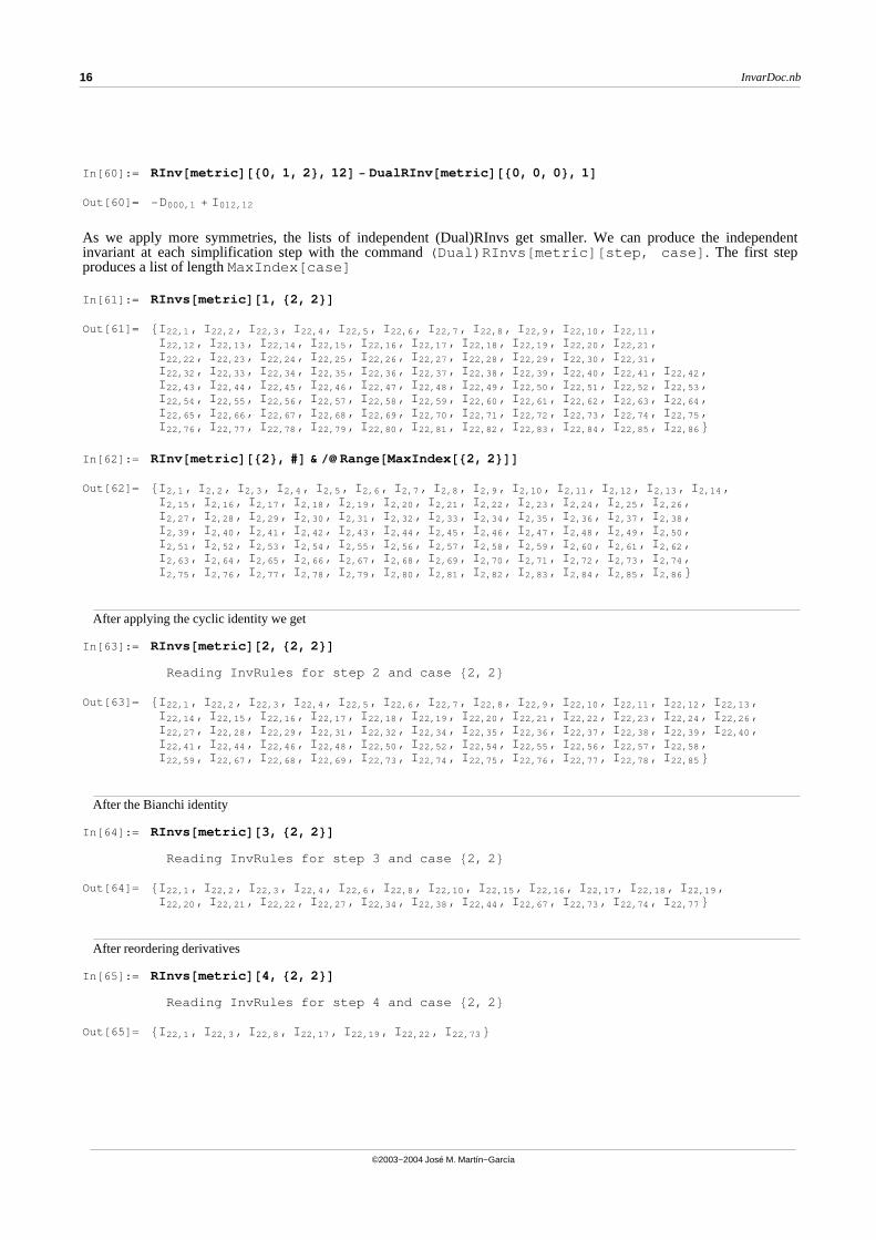
As we apply more symmetries, the lists of independent (Dual)RInvs get smaller. We can produce the independentinvariant at each simplification step with the command (Dual)RInvs[metric][step, case] . The first stepproduces a list of length MaxIndex[case]
In[61]:= RInvs@metricD@1, 82, 2<D
Out[61]= 8I 22,1 , I 22,2 , I 22,3 , I 22,4 , I 22,5 , I 22,6 , I 22,7 , I 22,8 , I 22,9 , I 22,10 , I 22,11 ,I 22,12 , I 22,13 , I 22,14 , I 22,15 , I 22,16 , I 22,17 , I 22,18 , I 22,19 , I 22,20 , I 22,21 ,I 22,22 , I 22,23 , I 22,24 , I 22,25 , I 22,26 , I 22,27 , I 22,28 , I 22,29 , I 22,30 , I 22,31 ,I 22,32 , I 22,33 , I 22,34 , I 22,35 , I 22,36 , I 22,37 , I 22,38 , I 22,39 , I 22,40 , I 22,41 , I 22,42 ,I 22,43 , I 22,44 , I 22,45 , I 22,46 , I 22,47 , I 22,48 , I 22,49 , I 22,50 , I 22,51 , I 22,52 , I 22,53 ,I 22,54 , I 22,55 , I 22,56 , I 22,57 , I 22,58 , I 22,59 , I 22,60 , I 22,61 , I 22,62 , I 22,63 , I 22,64 ,I 22,65 , I 22,66 , I 22,67 , I 22,68 , I 22,69 , I 22,70 , I 22,71 , I 22,72 , I 22,73 , I 22,74 , I 22,75 ,I 22,76 , I 22,77 , I 22,78 , I 22,79 , I 22,80 , I 22,81 , I 22,82 , I 22,83 , I 22,84 , I 22,85 , I 22,86 <
In[62]:= RInv@metricD@82<, #D & �� Range@MaxIndex@82, 2<DD
Out[62]= 8I 2,1 , I 2,2 , I 2,3 , I 2,4 , I 2,5 , I 2,6 , I 2,7 , I 2,8 , I 2,9 , I 2,10 , I 2,11 , I 2,12 , I 2,13 , I 2,14 ,I 2,15 , I 2,16 , I 2,17 , I 2,18 , I 2,19 , I 2,20 , I 2,21 , I 2,22 , I 2,23 , I 2,24 , I 2,25 , I 2,26 ,I 2,27 , I 2,28 , I 2,29 , I 2,30 , I 2,31 , I 2,32 , I 2,33 , I 2,34 , I 2,35 , I 2,36 , I 2,37 , I 2,38 ,I 2,39 , I 2,40 , I 2,41 , I 2,42 , I 2,43 , I 2,44 , I 2,45 , I 2,46 , I 2,47 , I 2,48 , I 2,49 , I 2,50 ,I 2,51 , I 2,52 , I 2,53 , I 2,54 , I 2,55 , I 2,56 , I 2,57 , I 2,58 , I 2,59 , I 2,60 , I 2,61 , I 2,62 ,I 2,63 , I 2,64 , I 2,65 , I 2,66 , I 2,67 , I 2,68 , I 2,69 , I 2,70 , I 2,71 , I 2,72 , I 2,73 , I 2,74 ,I 2,75 , I 2,76 , I 2,77 , I 2,78 , I 2,79 , I 2,80 , I 2,81 , I 2,82 , I 2,83 , I 2,84 , I 2,85 , I 2,86 <
After applying the cyclic identity we get
In[63]:= RInvs@metricD@2, 82, 2<D
Reading InvRules for step 2 and case 82, 2 <
Out[63]= 8I 22,1 , I 22,2 , I 22,3 , I 22,4 , I 22,5 , I 22,6 , I 22,7 , I 22,8 , I 22,9 , I 22,10 , I 22,11 , I 22,12 , I 22,13 ,I 22,14 , I 22,15 , I 22,16 , I 22,17 , I 22,18 , I 22,19 , I 22,20 , I 22,21 , I 22,22 , I 22,23 , I 22,24 , I 22,26 ,I 22,27 , I 22,28 , I 22,29 , I 22,31 , I 22,32 , I 22,34 , I 22,35 , I 22,36 , I 22,37 , I 22,38 , I 22,39 , I 22,40 ,I 22,41 , I 22,44 , I 22,46 , I 22,48 , I 22,50 , I 22,52 , I 22,54 , I 22,55 , I 22,56 , I 22,57 , I 22,58 ,I 22,59 , I 22,67 , I 22,68 , I 22,69 , I 22,73 , I 22,74 , I 22,75 , I 22,76 , I 22,77 , I 22,78 , I 22,85 <
After the Bianchi identity
In[64]:= RInvs@metricD@3, 82, 2<D
Reading InvRules for step 3 and case 82, 2 <
Out[64]= 8I 22,1 , I 22,2 , I 22,3 , I 22,4 , I 22,6 , I 22,8 , I 22,10 , I 22,15 , I 22,16 , I 22,17 , I 22,18 , I 22,19 ,I 22,20 , I 22,21 , I 22,22 , I 22,27 , I 22,34 , I 22,38 , I 22,44 , I 22,67 , I 22,73 , I 22,74 , I 22,77 <
After reordering derivatives
In[65]:= RInvs@metricD@4, 82, 2<D
Reading InvRules for step 4 and case 82, 2 <
Out[65]= 8I 22,1 , I 22,3 , I 22,8 , I 22,17 , I 22,19 , I 22,22 , I 22,73 <
16 InvarDoc.nb
©2003−2004 José M. Martín−García
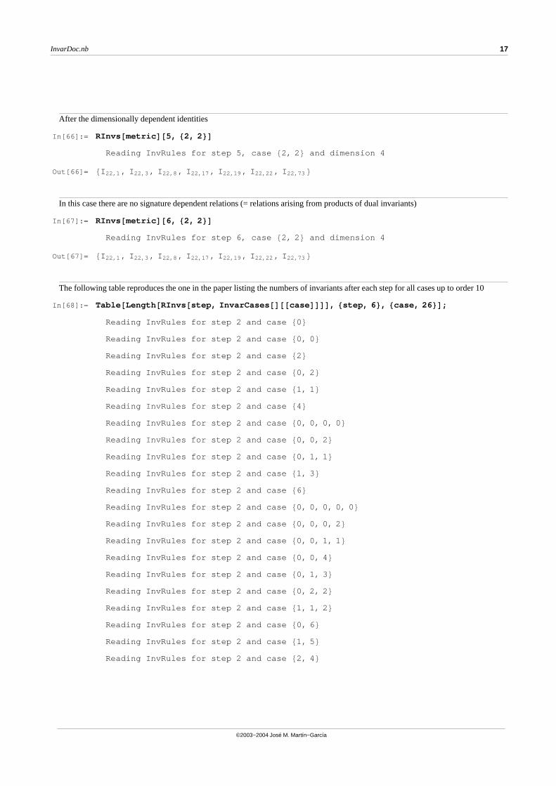
After the dimensionally dependent identities
In[66]:= RInvs@metricD@5, 82, 2<D
Reading InvRules for step 5, case 82, 2 < and dimension 4
Out[66]= 8I 22,1 , I 22,3 , I 22,8 , I 22,17 , I 22,19 , I 22,22 , I 22,73 <
In this case there are no signature dependent relations (= relations arising from products of dual invariants)
In[67]:= RInvs@metricD@6, 82, 2<D
Reading InvRules for step 6, case 82, 2 < and dimension 4
Out[67]= 8I 22,1 , I 22,3 , I 22,8 , I 22,17 , I 22,19 , I 22,22 , I 22,73 <
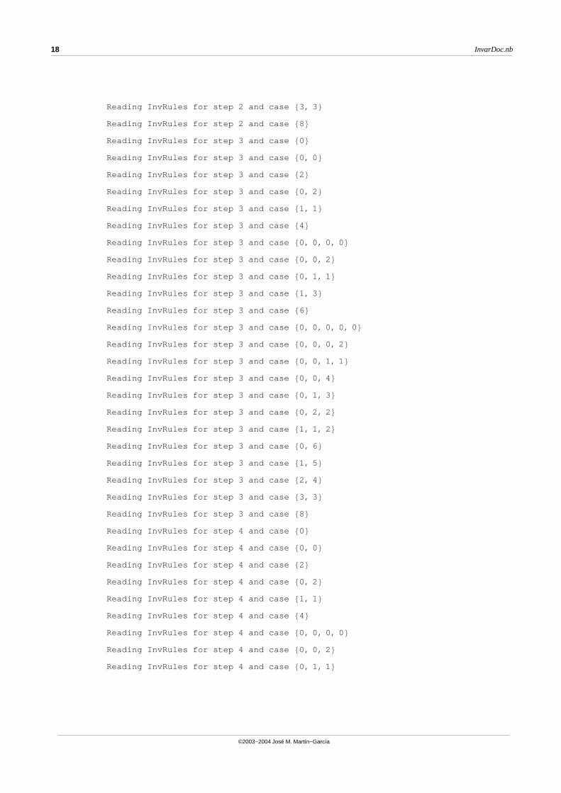
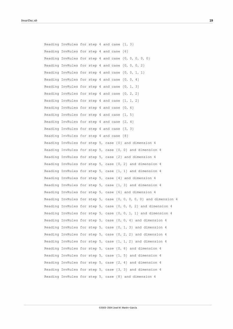
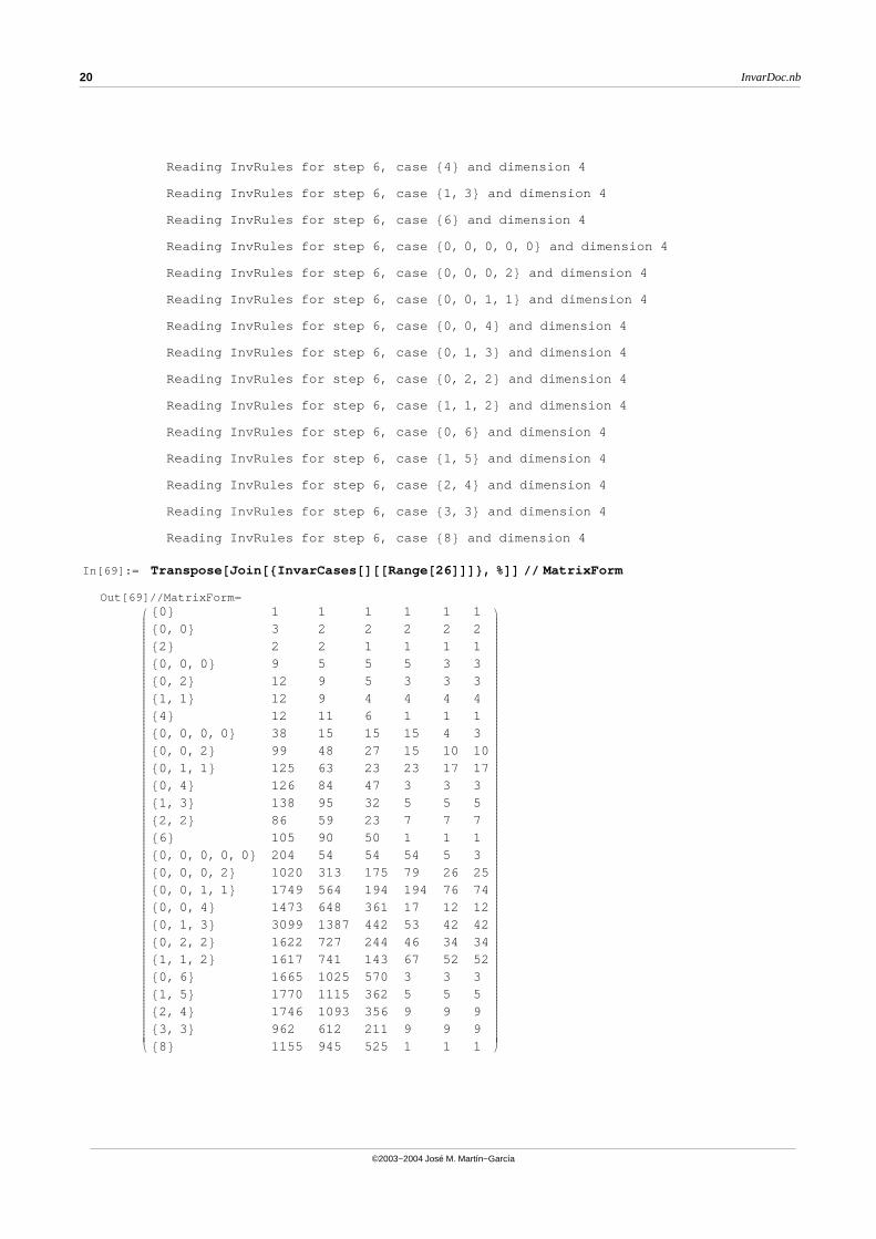
The following table reproduces the one in the paper listing the numbers of invariants after each step for all cases up to order 10
In[68]:= Table@Length@RInvs@step, InvarCases@D@@caseDDDD, 8step, 6<, 8case, 26<D;
Reading InvRules for step 2 and case 80<Reading InvRules for step 2 and case 80, 0 <Reading InvRules for step 2 and case 82<Reading InvRules for step 2 and case 80, 2 <Reading InvRules for step 2 and case 81, 1 <Reading InvRules for step 2 and case 84<Reading InvRules for step 2 and case 80, 0, 0, 0 <Reading InvRules for step 2 and case 80, 0, 2 <Reading InvRules for step 2 and case 80, 1, 1 <Reading InvRules for step 2 and case 81, 3 <Reading InvRules for step 2 and case 86<Reading InvRules for step 2 and case 80, 0, 0, 0, 0 <Reading InvRules for step 2 and case 80, 0, 0, 2 <Reading InvRules for step 2 and case 80, 0, 1, 1 <Reading InvRules for step 2 and case 80, 0, 4 <Reading InvRules for step 2 and case 80, 1, 3 <Reading InvRules for step 2 and case 80, 2, 2 <Reading InvRules for step 2 and case 81, 1, 2 <Reading InvRules for step 2 and case 80, 6 <Reading InvRules for step 2 and case 81, 5 <Reading InvRules for step 2 and case 82, 4 <
InvarDoc.nb 17
©2003−2004 José M. Martín−García
Reading InvRules for step 2 and case 83, 3 <Reading InvRules for step 2 and case 88<Reading InvRules for step 3 and case 80<Reading InvRules for step 3 and case 80, 0 <Reading InvRules for step 3 and case 82<Reading InvRules for step 3 and case 80, 2 <Reading InvRules for step 3 and case 81, 1 <Reading InvRules for step 3 and case 84<Reading InvRules for step 3 and case 80, 0, 0, 0 <Reading InvRules for step 3 and case 80, 0, 2 <Reading InvRules for step 3 and case 80, 1, 1 <Reading InvRules for step 3 and case 81, 3 <Reading InvRules for step 3 and case 86<Reading InvRules for step 3 and case 80, 0, 0, 0, 0 <Reading InvRules for step 3 and case 80, 0, 0, 2 <Reading InvRules for step 3 and case 80, 0, 1, 1 <Reading InvRules for step 3 and case 80, 0, 4 <Reading InvRules for step 3 and case 80, 1, 3 <Reading InvRules for step 3 and case 80, 2, 2 <Reading InvRules for step 3 and case 81, 1, 2 <Reading InvRules for step 3 and case 80, 6 <Reading InvRules for step 3 and case 81, 5 <Reading InvRules for step 3 and case 82, 4 <Reading InvRules for step 3 and case 83, 3 <Reading InvRules for step 3 and case 88<Reading InvRules for step 4 and case 80<Reading InvRules for step 4 and case 80, 0 <Reading InvRules for step 4 and case 82<Reading InvRules for step 4 and case 80, 2 <Reading InvRules for step 4 and case 81, 1 <Reading InvRules for step 4 and case 84<Reading InvRules for step 4 and case 80, 0, 0, 0 <Reading InvRules for step 4 and case 80, 0, 2 <Reading InvRules for step 4 and case 80, 1, 1 <
18 InvarDoc.nb
©2003−2004 José M. Martín−García
Reading InvRules for step 4 and case 81, 3 <Reading InvRules for step 4 and case 86<Reading InvRules for step 4 and case 80, 0, 0, 0, 0 <Reading InvRules for step 4 and case 80, 0, 0, 2 <Reading InvRules for step 4 and case 80, 0, 1, 1 <Reading InvRules for step 4 and case 80, 0, 4 <Reading InvRules for step 4 and case 80, 1, 3 <Reading InvRules for step 4 and case 80, 2, 2 <Reading InvRules for step 4 and case 81, 1, 2 <Reading InvRules for step 4 and case 80, 6 <Reading InvRules for step 4 and case 81, 5 <Reading InvRules for step 4 and case 82, 4 <Reading InvRules for step 4 and case 83, 3 <Reading InvRules for step 4 and case 88<Reading InvRules for step 5, case 80< and dimension 4
Reading InvRules for step 5, case 80, 0 < and dimension 4
Reading InvRules for step 5, case 82< and dimension 4
Reading InvRules for step 5, case 80, 2 < and dimension 4
Reading InvRules for step 5, case 81, 1 < and dimension 4
Reading InvRules for step 5, case 84< and dimension 4
Reading InvRules for step 5, case 81, 3 < and dimension 4
Reading InvRules for step 5, case 86< and dimension 4
Reading InvRules for step 5, case 80, 0, 0, 0, 0 < and dimension 4
Reading InvRules for step 5, case 80, 0, 0, 2 < and dimension 4
Reading InvRules for step 5, case 80, 0, 1, 1 < and dimension 4
Reading InvRules for step 5, case 80, 0, 4 < and dimension 4
Reading InvRules for step 5, case 80, 1, 3 < and dimension 4
Reading InvRules for step 5, case 80, 2, 2 < and dimension 4
Reading InvRules for step 5, case 81, 1, 2 < and dimension 4
Reading InvRules for step 5, case 80, 6 < and dimension 4
Reading InvRules for step 5, case 81, 5 < and dimension 4
Reading InvRules for step 5, case 82, 4 < and dimension 4
Reading InvRules for step 5, case 83, 3 < and dimension 4
Reading InvRules for step 5, case 88< and dimension 4
InvarDoc.nb 19
©2003−2004 José M. Martín−García
Reading InvRules for step 6, case 84< and dimension 4
Reading InvRules for step 6, case 81, 3 < and dimension 4
Reading InvRules for step 6, case 86< and dimension 4
Reading InvRules for step 6, case 80, 0, 0, 0, 0 < and dimension 4
Reading InvRules for step 6, case 80, 0, 0, 2 < and dimension 4
Reading InvRules for step 6, case 80, 0, 1, 1 < and dimension 4
Reading InvRules for step 6, case 80, 0, 4 < and dimension 4
Reading InvRules for step 6, case 80, 1, 3 < and dimension 4
Reading InvRules for step 6, case 80, 2, 2 < and dimension 4
Reading InvRules for step 6, case 81, 1, 2 < and dimension 4
Reading InvRules for step 6, case 80, 6 < and dimension 4
Reading InvRules for step 6, case 81, 5 < and dimension 4
Reading InvRules for step 6, case 82, 4 < and dimension 4
Reading InvRules for step 6, case 83, 3 < and dimension 4
Reading InvRules for step 6, case 88< and dimension 4
In[69]:= Transpose@Join@8InvarCases@D@@Range@26DDD<, %DD �� MatrixForm
Out[69]//MatrixForm=
i
k
jjjjjjjjjjjjjjjjjjjjjjjjjjjjjjjjjjjjjjjjjjjjjjjjjjjjjjjjjjjjjjjjjjjjjjjjjjjjjjjjjjjjjjjjjjjjjjjjjjjjjjjjjjjjjjjjjjjjjjjjjjjjj
80< 1 1 1 1 1 180, 0 < 3 2 2 2 2 282< 2 2 1 1 1 180, 0, 0 < 9 5 5 5 3 380, 2 < 12 9 5 3 3 381, 1 < 12 9 4 4 4 484< 12 11 6 1 1 180, 0, 0, 0 < 38 15 15 15 4 380, 0, 2 < 99 48 27 15 10 1080, 1, 1 < 125 63 23 23 17 1780, 4 < 126 84 47 3 3 381, 3 < 138 95 32 5 5 582, 2 < 86 59 23 7 7 786< 105 90 50 1 1 180, 0, 0, 0, 0 < 204 54 54 54 5 380, 0, 0, 2 < 1020 313 175 79 26 2580, 0, 1, 1 < 1749 564 194 194 76 7480, 0, 4 < 1473 648 361 17 12 1280, 1, 3 < 3099 1387 442 53 42 4280, 2, 2 < 1622 727 244 46 34 3481, 1, 2 < 1617 741 143 67 52 5280, 6 < 1665 1025 570 3 3 381, 5 < 1770 1115 362 5 5 582, 4 < 1746 1093 356 9 9 983, 3 < 962 612 211 9 9 988< 1155 945 525 1 1 1
y
{
zzzzzzzzzzzzzzzzzzzzzzzzzzzzzzzzzzzzzzzzzzzzzzzzzzzzzzzzzzzzzzzzzzzzzzzzzzzzzzzzzzzzzzzzzzzzzzzzzzzzzzzzzzzzzzzzzzzzzzzzzzzzz
20 InvarDoc.nb
©2003−2004 José M. Martín−García

The simplified notation RInvs[metric][step, n] is automatically translated into RInvs[metric][step, {0, ...n , 0}] , for backwards compatibility with Invar 1. For instance, these are all the algebraic invariants after step 3 with degree 6 (case {0,0,0,0,0,0}):
In[70]:= RInvs@metricD@3, 6D
Reading InvRules for step 2 and case 80, 0, 0, 0, 0, 0 <Reading InvRules for step 3 and case 80, 0, 0, 0, 0, 0 <
Out[70]= 8I 000000,1 , I 000000,2 , I 000000,3 , I 000000,4 , I 000000,6 , I 000000,8 , I 000000,9 , I 000000,11 , I 000000,13 ,I 000000,14 , I 000000,16 , I 000000,17 , I 000000,18 , I 000000,19 , I 000000,22 , I 000000,23 , I 000000,25 ,I 000000,27 , I 000000,32 , I 000000,34 , I 000000,36 , I 000000,38 , I 000000,40 , I 000000,45 , I 000000,47 ,I 000000,49 , I 000000,50 , I 000000,52 , I 000000,57 , I 000000,60 , I 000000,65 , I 000000,66 , I 000000,69 ,I 000000,71 , I 000000,74 , I 000000,76 , I 000000,77 , I 000000,84 , I 000000,86 , I 000000,87 , I 000000,88 ,I 000000,91 , I 000000,94 , I 000000,95 , I 000000,97 , I 000000,101 , I 000000,103 , I 000000,108 , I 000000,110 ,I 000000,112 , I 000000,114 , I 000000,117 , I 000000,119 , I 000000,136 , I 000000,140 , I 000000,143 , I 000000,147 ,I 000000,149 , I 000000,151 , I 000000,156 , I 000000,165 , I 000000,167 , I 000000,174 , I 000000,176 , I 000000,178 ,I 000000,180 , I 000000,183 , I 000000,187 , I 000000,189 , I 000000,191 , I 000000,196 , I 000000,208 , I 000000,213 ,I 000000,216 , I 000000,221 , I 000000,223 , I 000000,229 , I 000000,231 , I 000000,233 , I 000000,235 ,I 000000,240 , I 000000,242 , I 000000,244 , I 000000,245 , I 000000,247 , I 000000,252 , I 000000,255 ,I 000000,260 , I 000000,261 , I 000000,264 , I 000000,266 , I 000000,268 , I 000000,270 , I 000000,275 ,I 000000,292 , I 000000,296 , I 000000,298 , I 000000,304 , I 000000,309 , I 000000,312 , I 000000,331 ,I 000000,334 , I 000000,342 , I 000000,344 , I 000000,346 , I 000000,348 , I 000000,349 , I 000000,353 ,I 000000,359 , I 000000,362 , I 000000,372 , I 000000,374 , I 000000,379 , I 000000,381 , I 000000,383 , I 000000,385 ,I 000000,393 , I 000000,395 , I 000000,400 , I 000000,402 , I 000000,404 , I 000000,406 , I 000000,409 ,I 000000,411 , I 000000,428 , I 000000,432 , I 000000,435 , I 000000,439 , I 000000,441 , I 000000,443 ,I 000000,448 , I 000000,457 , I 000000,459 , I 000000,464 , I 000000,466 , I 000000,468 , I 000000,470 ,I 000000,474 , I 000000,478 , I 000000,480 , I 000000,484 , I 000000,492 , I 000000,497 , I 000000,499 ,I 000000,503 , I 000000,505 , I 000000,510 , I 000000,533 , I 000000,535 , I 000000,539 , I 000000,544 ,I 000000,561 , I 000000,569 , I 000000,625 , I 000000,627 , I 000000,629 , I 000000,633 , I 000000,650 ,I 000000,655 , I 000000,658 , I 000000,665 , I 000000,670 , I 000000,672 , I 000000,701 , I 000000,703 ,I 000000,708 , I 000000,712 , I 000000,714 , I 000000,716 , I 000000,719 , I 000000,725 , I 000000,732 ,I 000000,738 , I 000000,740 , I 000000,742 , I 000000,749 , I 000000,751 , I 000000,754 , I 000000,765 ,I 000000,767 , I 000000,772 , I 000000,782 , I 000000,791 , I 000000,797 , I 000000,802 , I 000000,828 ,I 000000,829 , I 000000,839 , I 000000,864 , I 000000,869 , I 000000,898 , I 000000,928 , I 000000,930 ,I 000000,935 , I 000000,937 , I 000000,939 , I 000000,941 , I 000000,944 , I 000000,946 , I 000000,963 ,I 000000,967 , I 000000,970 , I 000000,974 , I 000000,976 , I 000000,978 , I 000000,983 , I 000000,993 ,I 000000,998 , I 000000,1001 , I 000000,1003 , I 000000,1006 , I 000000,1009 , I 000000,1011 , I 000000,1015 ,I 000000,1023 , I 000000,1028 , I 000000,1030 , I 000000,1045 , I 000000,1048 , I 000000,1053 , I 000000,1058 ,I 000000,1068 , I 000000,1073 , I 000000,1076 , I 000000,1081 , I 000000,1083 , I 000000,1131 , I 000000,1142 ,I 000000,1146 , I 000000,1148 , I 000000,1153 , I 000000,1158 , I 000000,1161 , I 000000,1179 , I 000000,1182 ,I 000000,1190 , I 000000,1192 , I 000000,1194 , I 000000,1201 , I 000000,1203 , I 000000,1204 , I 000000,1213 ,I 000000,1219 , I 000000,1221 , I 000000,1223 , I 000000,1478 , I 000000,1480 , I 000000,1482 , I 000000,1486 ,I 000000,1488 , I 000000,1502 , I 000000,1504 , I 000000,1508 , I 000000,1510 , I 000000,1519 , I 000000,1523 ,I 000000,1530 , I 000000,1541 , I 000000,1542 , I 000000,1548 , I 000000,1561 , I 000000,1563 , I 000000,1572 ,I 000000,1576 , I 000000,1577 , I 000000,1579 , I 000000,1582 , I 000000,1586 , I 000000,1588 , I 000000,1596 <
Similar shorthands are available for other commands, such as MaxIndex or RInv
In[71]:= 8MaxIndex@7D, MaxIndex@80, 0, 0, 0, 0, 0, 0<D<
Out[71]= 816532, 16532 <
In[72]:= RInv@metricD@4, 1D
Out[72]= I 0000,1
InvarDoc.nb 21
©2003−2004 José M. Martín−García
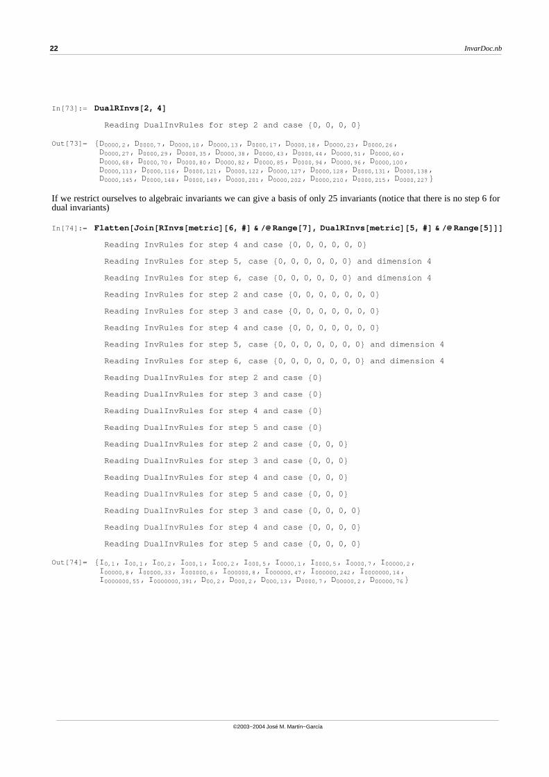
In[73]:= DualRInvs@2, 4D
Reading DualInvRules for step 2 and case 80, 0, 0, 0 <
Out[73]= 8D0000,2 , D 0000,7 , D 0000,10 , D 0000,13 , D 0000,17 , D 0000,18 , D 0000,23 , D 0000,26 ,D0000,27 , D 0000,29 , D 0000,35 , D 0000,38 , D 0000,43 , D 0000,44 , D 0000,51 , D 0000,60 ,D0000,68 , D 0000,70 , D 0000,80 , D 0000,82 , D 0000,85 , D 0000,94 , D 0000,96 , D 0000,100 ,D0000,113 , D 0000,116 , D 0000,121 , D 0000,122 , D 0000,127 , D 0000,128 , D 0000,131 , D 0000,138 ,D0000,145 , D 0000,148 , D 0000,149 , D 0000,201 , D 0000,202 , D 0000,210 , D 0000,215 , D 0000,227 <
If we restrict ourselves to algebraic invariants we can give a basis of only 25 invariants (notice that there is no step 6 fordual invariants)
In[74]:= Flatten@Join@RInvs@metricD@6, #D & �� Range@7D, DualRInvs@metricD@5, #D & �� Range@5DDD
Reading InvRules for step 4 and case 80, 0, 0, 0, 0, 0 <Reading InvRules for step 5, case 80, 0, 0, 0, 0, 0 < and dimension 4
Reading InvRules for step 6, case 80, 0, 0, 0, 0, 0 < and dimension 4
Reading InvRules for step 2 and case 80, 0, 0, 0, 0, 0, 0 <Reading InvRules for step 3 and case 80, 0, 0, 0, 0, 0, 0 <Reading InvRules for step 4 and case 80, 0, 0, 0, 0, 0, 0 <Reading InvRules for step 5, case 80, 0, 0, 0, 0, 0, 0 < and dimension 4
Reading InvRules for step 6, case 80, 0, 0, 0, 0, 0, 0 < and dimension 4
Reading DualInvRules for step 2 and case 80<Reading DualInvRules for step 3 and case 80<Reading DualInvRules for step 4 and case 80<Reading DualInvRules for step 5 and case 80<Reading DualInvRules for step 2 and case 80, 0, 0 <Reading DualInvRules for step 3 and case 80, 0, 0 <Reading DualInvRules for step 4 and case 80, 0, 0 <Reading DualInvRules for step 5 and case 80, 0, 0 <Reading DualInvRules for step 3 and case 80, 0, 0, 0 <Reading DualInvRules for step 4 and case 80, 0, 0, 0 <Reading DualInvRules for step 5 and case 80, 0, 0, 0 <
Out[74]= 8I 0,1 , I 00,1 , I 00,2 , I 000,1 , I 000,2 , I 000,5 , I 0000,1 , I 0000,5 , I 0000,7 , I 00000,2 ,I 00000,8 , I 00000,33 , I 000000,6 , I 000000,8 , I 000000,47 , I 000000,242 , I 0000000,14 ,I 0000000,55 , I 0000000,391 , D 00,2 , D 000,2 , D 000,13 , D 0000,7 , D 00000,2 , D 00000,76 <
22 InvarDoc.nb
©2003−2004 José M. Martín−García
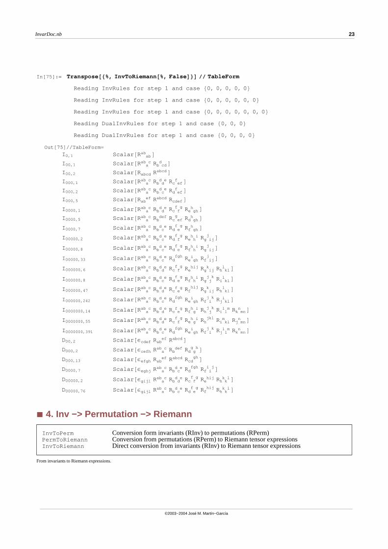
In[75]:= Transpose@8%, InvToRiemann@%, FalseD<D �� TableForm
Reading InvRules for step 1 and case 80, 0, 0, 0, 0 <Reading InvRules for step 1 and case 80, 0, 0, 0, 0, 0 <Reading InvRules for step 1 and case 80, 0, 0, 0, 0, 0, 0 <Reading DualInvRules for step 1 and case 80, 0, 0 <Reading DualInvRules for step 1 and case 80, 0, 0, 0 <
Out[75]//TableForm=
I 0,1 Scalar @R abab D
I 00,1 Scalar @R aab c Rb cd
d DI 00,2 Scalar @Rabcd Rabcd DI 000,1 Scalar @R a
ab c Rb dd e Rc ef
f DI 000,2 Scalar @R a
ab c Rb cd e Rd ef
f DI 000,5 Scalar @Rab
ef Rabcd Rcdef DI 0000,1 Scalar @R a
ab c Rb dd e Rc f
f g Re ghh D
I 0000,5 Scalar @R aab c Rb
def Rc efg Rd gh
h DI 0000,7 Scalar @R a
ab c Rb cd e Rd e
f g Rf ghh D
I 00000,2 Scalar @R aab c Rb c
d e Rd ff g Re h
h i Rg ijj D
I 00000,8 Scalar @R aab c Rb c
d e Rd ef g Rf h
h i Rg ijj D
I 00000,33 Scalar @R aab c Rb c
d e Rdfgh Re gh
i Rf ijj D
I 000000,6 Scalar @R aab c Rb d
d e Rc ff g Re
hij Rg ijk Rh kl
l DI 000000,8 Scalar @R a
ab c Rb cd e Rd e
f g Rf hh i Rg j
j k Ri kll D
I 000000,47 Scalar @R aab c Rb d
d e Rc ef g Rf
hij Rg ijk Rh kl
l DI 000000,242 Scalar @R a
ab c Rb cd e Rd
fgh Re ghi Rf i
j k Rj kll D
I 0000000,14 Scalar @R aab c Rb d
d e Rc ef g Rf g
h i Rh jj k Ri l
l m Rk mnn D
I 0000000,55 Scalar @R aab c Rb d
d e Rc ff g Re g
h i Rhjkl Ri kl
m Rj mnn D
I 0000000,391 Scalar @R aab c Rb c
d e Rdfgh Re gh
i Rf ij k Rj l
l m Rk mnn D
D00,2 Scalar @Εcdef Rabef Rabcd D
D000,2 Scalar @Εcefh R aab c Rb
def Rd gg h D
D000,13 Scalar @Εefgh Rabef Rabcd Rcd
gh DD0000,7 Scalar @Εeghj R a
ab c Rb cd e Rd
fgh Rf ii j D
D00000,2 Scalar @Εgijl R aab c Rb d
d e Rc ff g Re
hij Rh kk l D
D00000,76 Scalar @Εgijl R aab c Rb c
d e Rd ef g Rf
hij Rh kk l D
à 4. Inv −> Permutation −> Riemann
InvToPerm Conversion form invariants (RInv) to permutations (RPerm)PermToRiemann Conversion from permutations (RPerm) to Riemann tensor expressionsInvToRiemann Direct conversion from invariants (RInv) to Riemann tensor expressions
From invariants to Riemann expressions.
InvarDoc.nb 23
©2003−2004 José M. Martín−García
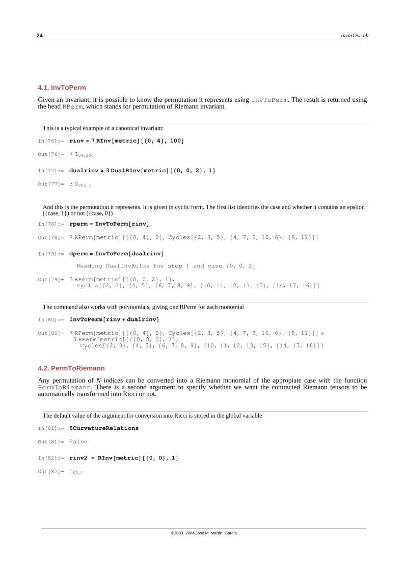
4.1. InvToPerm
Given an invariant, it is possible to know the permutation it represents using InvToPerm . The result is returned usingthe head RPerm, which stands for permutation of Riemann invariant.
This is a typical example of a canonical invariant:
In[76]:= rinv = 7 RInv@metricD@80, 4<, 100D
Out[76]= 7 I 04,100
In[77]:= dualrinv = 3 DualRInv@metricD@80, 0, 2<, 1D
Out[77]= 3 D002,1
And this is the permutation it represents. It is given in cyclic form. The first list identifies the case and whether it contains an epsilon ({case, 1}) or not ({case, 0})
In[78]:= rperm = InvToPerm@rinvD
Out[78]= 7 RPerm@metric D@880, 4 <, 0 <, Cycles @82, 3, 5 <, 84, 7, 9, 10, 6 <, 88, 11 <DD
In[79]:= dperm = InvToPerm@dualrinvD
Reading DualInvRules for step 1 and case 80, 0, 2 <
Out[79]= 3 RPerm@metric D@880, 0, 2 <, 1 <,Cycles @82, 3 <, 84, 5 <, 86, 7, 8, 9 <, 810, 11, 12, 13, 15 <, 814, 17, 16 <DD
The command also works with polynomials, giving one RPerm for each monomial
In[80]:= InvToPerm@rinv + dualrinvD
Out[80]= 7 RPerm@metric D@880, 4 <, 0 <, Cycles @82, 3, 5 <, 84, 7, 9, 10, 6 <, 88, 11 <DD +
3 RPerm@metric D@880, 0, 2 <, 1 <,Cycles @82, 3 <, 84, 5 <, 86, 7, 8, 9 <, 810, 11, 12, 13, 15 <, 814, 17, 16 <DD
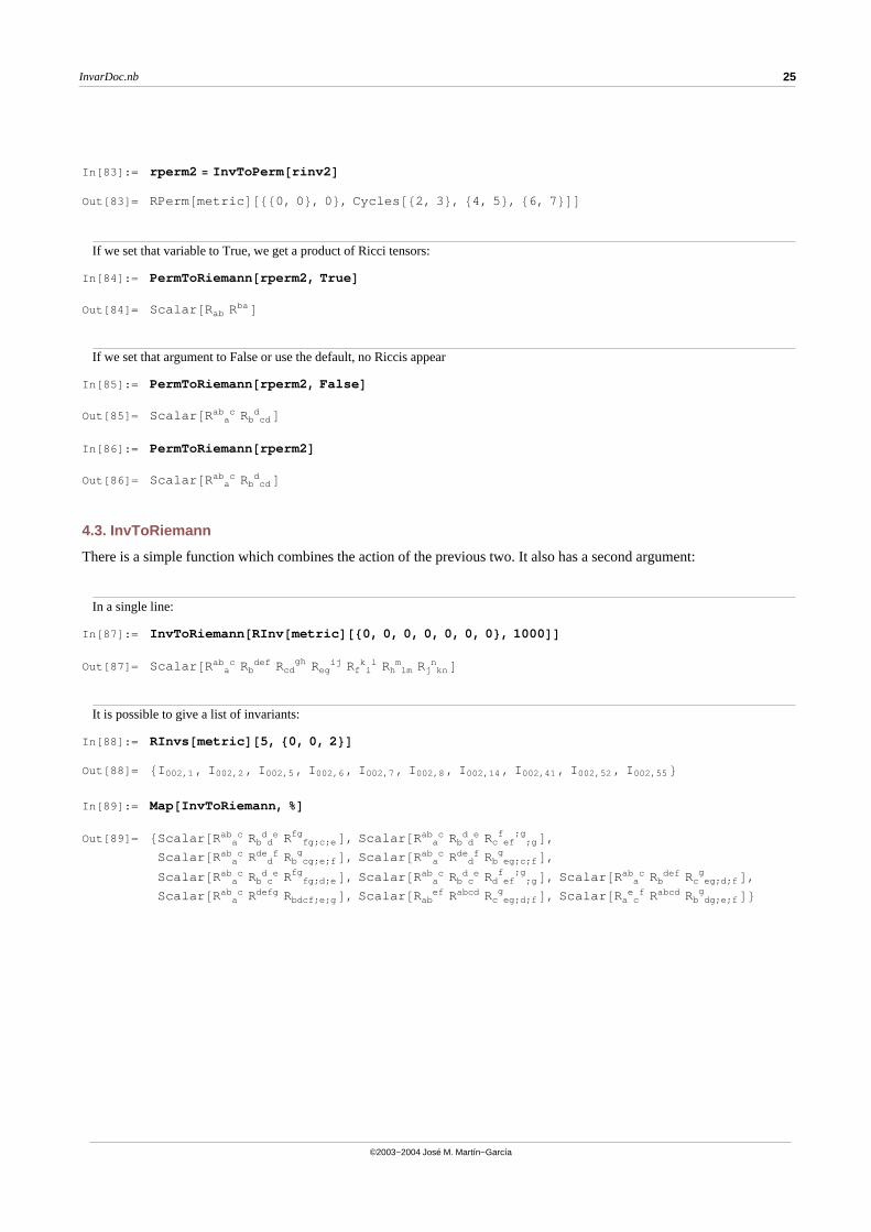
4.2. PermToRiemann
Any permutation of N indices can be converted into a Riemann monomial of the appropiate case with the functionPermToRiemann . There is a second argument to specify whether we want the contracted Riemann tensors to beautomatically transformed into Ricci or not.
The default value of the argument for conversion into Ricci is stored in the global variable
In[81]:= $CurvatureRelations
Out[81]= False
In[82]:= rinv2 = RInv@metricD@80, 0<, 1D
Out[82]= I 00,1
24 InvarDoc.nb
©2003−2004 José M. Martín−García
In[83]:= rperm2 = InvToPerm@rinv2D
Out[83]= RPerm@metric D@880, 0 <, 0 <, Cycles @82, 3 <, 84, 5 <, 86, 7 <DD
If we set that variable to True, we get a product of Ricci tensors:
In[84]:= PermToRiemann@rperm2, TrueD
Out[84]= Scalar @Rab Rba D
If we set that argument to False or use the default, no Riccis appear
In[85]:= PermToRiemann@rperm2, FalseD
Out[85]= Scalar @R aab c Rb cd
d D
In[86]:= PermToRiemann@rperm2D
Out[86]= Scalar @R aab c Rb cd
d D
4.3. InvToRiemann
There is a simple function which combines the action of the previous two. It also has a second argument:
In a single line:
In[87]:= InvToRiemann@RInv@metricD@80, 0, 0, 0, 0, 0, 0<, 1000DD
Out[87]= Scalar @R aab c Rb
def Rcdgh Reg
ij Rf ik l Rh lm
m Rj knn D
It is possible to give a list of invariants:
In[88]:= RInvs@metricD@5, 80, 0, 2<D
Out[88]= 8I 002,1 , I 002,2 , I 002,5 , I 002,6 , I 002,7 , I 002,8 , I 002,14 , I 002,41 , I 002,52 , I 002,55 <
In[89]:= Map@InvToRiemann, %D
Out[89]= 8Scalar @R aab c Rb d
d e R fg;c;efg D, Scalar @R a
ab c Rb dd e Rc ef ;g
f ;g D,
Scalar @R aab c R d
de f Rb cg;e;fg D, Scalar @R a
ab c R dde f Rb eg;c;f
g D,
Scalar @R aab c Rb c
d e R fg;d;efg D, Scalar @R a
ab c Rb cd e Rd ef ;g
f ;g D, Scalar @R aab c Rb
def Rc eg;d;fg D,
Scalar @R aab c Rdefg Rbdcf;e;g D, Scalar @Rab
ef Rabcd Rc eg;d;fg D, Scalar @Ra c
e f Rabcd Rb dg;e;fg D<
InvarDoc.nb 25
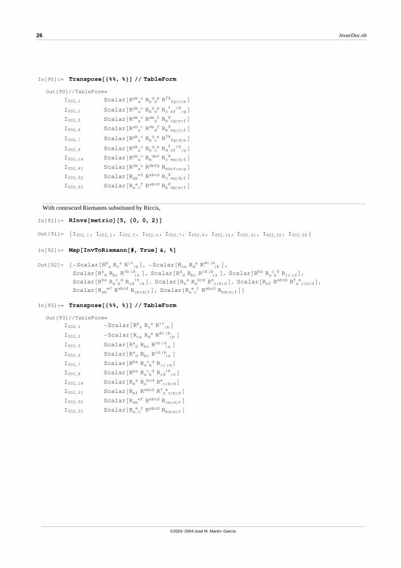
©2003−2004 José M. Martín−García
In[90]:= Transpose@8%%, %<D �� TableForm
Out[90]//TableForm=
I 002,1 Scalar @R aab c Rb d
d e R fg;c;efg D
I 002,2 Scalar @R aab c Rb d
d e Rc ef ;gf ;g D
I 002,5 Scalar @R aab c R d
de f Rb cg;e;fg D
I 002,6 Scalar @R aab c R d
de f Rb eg;c;fg D
I 002,7 Scalar @R aab c Rb c
d e R fg;d;efg D
I 002,8 Scalar @R aab c Rb c
d e Rd ef ;gf ;g D
I 002,14 Scalar @R aab c Rb
def Rc eg;d;fg D
I 002,41 Scalar @R aab c Rdefg Rbdcf;e;g D
I 002,52 Scalar @Rabef Rabcd Rc eg;d;f
g DI 002,55 Scalar @Ra c
e f Rabcd Rb dg;e;fg D
With contracted Riemanns substituted by Riccis,
In[91]:= RInvs@metricD@5, 80, 0, 2<D
Out[91]= 8I 002,1 , I 002,2 , I 002,5 , I 002,6 , I 002,7 , I 002,8 , I 002,14 , I 002,41 , I 002,52 , I 002,55 <
In[92]:= Map@InvToRiemann@#, TrueD &, %D
Out[92]= 8-Scalar @R ab Rc
a R ;b;c D, -Scalar @Rca Rd
a R ;bdc ;b D,
Scalar @R da Rbc R ;a
cb ;d D, Scalar @R da Rbc R ;a
cd ;b D, Scalar @Rba Ra bc d R;c ;d D,
Scalar @Rba Ra bc d Rcd ;e
;e D, Scalar @Rea Ra
bcd R c;b;de D, Scalar @Ref Rabcd R a c;b;d
f e D,Scalar @Rab
ef Rabcd Rce;d;f D, Scalar @Ra ce f Rabcd Rbd;e;f D<
In[93]:= Transpose@8%%, %<D �� TableForm
Out[93]//TableForm=
I 002,1 -Scalar @R ab Rc
a R ;b;c D
I 002,2 -Scalar @Rca Rda R ;b
dc ;b DI 002,5 Scalar @R d
a Rbc R ;acb ;d D
I 002,6 Scalar @R da Rbc R ;a
cd ;b DI 002,7 Scalar @Rba Ra b
c d R;c ;d DI 002,8 Scalar @Rba Ra b
c d Rcd ;e;e D
I 002,14 Scalar @Rea Ra
bcd R c;b;de D
I 002,41 Scalar @Ref Rabcd R a c;b;df e D
I 002,52 Scalar @Rabef Rabcd Rce;d;f D
I 002,55 Scalar @Ra ce f Rabcd Rbd;e;f D
26 InvarDoc.nb
©2003−2004 José M. Martín−García
Note that we have got a minus sign. This is because the invariants are sorted with respect to their Riemann−only expression:
à 5. Riemann −> Permutation −> Inv
RiemannToPerm Conversion from Riemann tensor expressions into permutations (RPerm)PermToInv Strong Conversion from permutations (RPerm) into invariants (RInv)RiemannToInv Direct conversion from Riemann tensor expressions into invariants (RInv)
From Riemann expressions to invariants.
5.1. RiemannToPerm
The function RiemannToPerm converts all Riemann scalars of a given metric (or list of metrics) into their canonicalpermutations:
Suppose we start from this simple expression:
In[94]:= rexpr = RiemannCD@a, b, c, dD RiemannCD@-a, -b, -c, -dD +
6 RiemannCD@e, f, -c, -dD RiemannCD@-a, -b, -e, -fD epsilonmetric@a, b, c, dD
Out[94]= Rabcd Rabcd+ 6 Ε
abcd Rabef R cdef
Then we can transform all terms into their canonical permutations,
In[95]:= rperm = RiemannToPerm@rexprD
Out[95]= RPerm@metric D@880, 0 <, 0 <, Cycles @82, 3, 5 <, 84, 7, 6 <DD +
6 RPerm@metric D@880, 0 <, 1 <, Cycles @82, 3, 5 <, 84, 7, 9, 6 <, 88, 11, 10 <DD
that is, not the permutations which would regenerate the previous objects:
In[96]:= PermToRiemann@rpermD
Out[96]= Scalar @Rabcd Rabcd D + 6 Scalar @Εcdef Rabef Rabcd D
5.2. PermToInv
This function uses the stored tables of results to identify the index corresponding to a given canonical permutation.
Example:
In[97]:= PermToInv@rpermD
Out[97]= 6 D00,2 + I 00,2
InvarDoc.nb 27
©2003−2004 José M. Martín−García
This function only works with canonical permutations:
In[98]:= InvToPerm@RInv@metricD@80, 2<, 3DD
Out[98]= RPerm@metric D@880, 2 <, 0 <, Cycles @82, 3 <, 84, 5 <, 86, 7, 8, 9 <DD
In[99]:= PermToInv@%D
Out[99]= I 02,3
We rewrite the cycles in a different form
In[100]:=RPerm@metricD@880, 2<, 0<, Cycles@83, 2<, 84, 5<, 86, 7, 8, 9<DD
Out[100]=RPerm@metric D@880, 2 <, 0 <, Cycles @83, 2 <, 84, 5 <, 86, 7, 8, 9 <DD
but now PermToInv does not work, because the new permutation is not canonical
In[101]:=PermToInv@%D
Out[101]=Cycles @83, 2 <, 84, 5 <, 86, 7, 8, 9 <D
5.3. RiemannToInv
Combined function:
Simple example:
In[102]:=RiemannToInv@rexprD
Out[102]=6 D00,2 + I 00,2
à 6. Simplification
6.1. InvSimplify
Once we have converted any Riemann expression into invariants with heads RInv and DualRInv , then we can"simplify" the expression by using the multiterm symmetries described above (steps 2, 3 and 4 of the simplificationprocess). We use quotes because in many cases a single monomial is expanded into a large polynomial, its canonicalform in the basis we have chosen, and this can be hardly called simplification. However, if an expression is equivalent tozero, the function InvSimplify will find it.
28 InvarDoc.nb
©2003−2004 José M. Martín−García
Example:
In[103]:=rinv = RInv@metricD@80, 0, 0, 0, 0<, 100D
Out[103]=I 00000,100
At level 1 nothing happens:
In[104]:=InvSimplify@rinv, 1D
Out[104]=I 00000,100
At level 2 the cyclic identity is used. Note that the degree does not change, but the indexes of the invariants decrease:
In[105]:=InvSimplify@rinv, 2D
Out[105]=-I 00000,97 + I 00000,99
We skip levels 3 and 4 becasue there are no derivatives in this example. At level 5 we use dimensionally dependent identities for dimension 4:
In[106]:=InvSimplify@rinv, 5D �� Expand
Out[106]=
-11 I 0,1
5
�������������������96
+79��������96
I 0,13 I 00,1 -
1�����8
I 0,1 I 00,12
-1
�����������192
I 0,13 I 00,2 +
5��������32
I 0,1 I 00,1 I 00,2 -1
��������64
I 0,1 I 00,22
+
5�����3
I 0,12 I 000,1 +
I 00,1 I 000,1�����������������������������
6+
I 00,2 I 000,1�����������������������������
6+
1�����4
I 0,12 I 000,2 -
I 00,1 I 000,2�����������������������������
2-
I 00,2 I 000,2�����������������������������
8-
1��������32
I 0,12 I 000,5 +
3 I 0,1 I 0000,1����������������������������������
2-
I 0,1 I 0000,5�����������������������������
8-
3 I 0,1 I 0000,7����������������������������������
4+
I 0,1 I 0000,21�������������������������������
32+ I 00000,2
At level 6 we use signature dependent identities expressing RInv[{0,0,0,0}, 21] in terms of DualRInv[{0,0}, 2] squared:
In[107]:=InvSimplify@rinv, 6D �� Expand
Out[107]=
-1
�����������512
D00,22 I 0,1 -
49 I 0,15
�������������������384
+91��������96
I 0,13 I 00,1 -
3��������16
I 0,1 I 00,12
-1
��������48
I 0,13 I 00,2 +
5��������32
I 0,1 I 00,1 I 00,2 -1
�����������128
I 0,1 I 00,22
+5�����3
I 0,12 I 000,1 +
I 00,1 I 000,1�����������������������������
6+
I 00,2 I 000,1�����������������������������
6-
I 00,1 I 000,2�����������������������������
2-
I 00,2 I 000,2�����������������������������
8-
1��������96
I 0,12 I 000,5 +
11 I 0,1 I 0000,1�������������������������������������
8-
I 0,1 I 0000,7�����������������������������
2+ I 00000,2
Another example, with derivatives and involving dual relations
InvarDoc.nb 29
©2003−2004 José M. Martín−García
In[108]:=diffrinv = RInv@metricD@80, 0, 1, 1<, 800D
Out[108]=I 0011,800
In[109]:=InvSimplify@diffrinv, 2D
Out[109]=
-I 0011,793����������������������
2
In[110]:=InvSimplify@diffrinv, 3D
Out[110]=
-I 0011,368����������������������
2+
I 0011,369����������������������
2
In[111]:=InvSimplify@diffrinv, 4D
Out[111]=
-I 0011,368����������������������
2+
I 0011,369����������������������
2
In[112]:=InvSimplify@diffrinv, 5D
Out[112]=
-3
��������32
I 0,12 I 11,1 +
3 I 00,1 I 11,1�������������������������������
8-
I 00,2 I 11,1���������������������������
32+
3�����8
I 0,12 I 11,4 -
3 I 00,1 I 11,4�������������������������������
2+
I 00,2 I 11,4���������������������������
8-
3�����8
I 0,12 I 11,5 +
3 I 00,1 I 11,5�������������������������������
2-
I 00,2 I 11,5���������������������������
8+
I 0,1 I 011,1���������������������������
8+
I 0,1 I 011,2���������������������������
2+
I 0,1 I 011,3���������������������������
2+
I 0,1 I 011,8 -I 0,1 I 011,9���������������������������
2- I 0,1 I 011,10 -
I 0,1 I 011,11�����������������������������
2+
I 0011,1������������������
4+ I 0011,2 + I 0011,3 +
2 I 0011,10 - I 0011,11 - 2 I 0011,12 - I 0011,13 -I 0011,23��������������������
4- I 0011,24 - I 0011,25 - 2 I 0011,42 +
I 0011,43 + 2 I 0011,44 + I 0011,50 +I 0011,125����������������������
2+
I 0011,362����������������������
2- I 0011,363 +
I 0011,367����������������������
2-
I 0011,368����������������������
2
In[113]:=InvSimplify@diffrinv, 6D
Out[113]=
-1
��������16
D00,2 D11,1 -I 0011,367����������������������
2
Simplification of a dual invariant
In[114]:=dualrinv = DualRInv@metricD@81, 3<, 3D
Out[114]=D13,3
30 InvarDoc.nb
©2003−2004 José M. Martín−García
In[115]:=InvSimplify@dualrinv, 2D
Reading DualInvRules for step 2 and case 81, 3 <Out[115]=
D13,3
In[116]:=InvSimplify@dualrinv, 3D
Reading DualInvRules for step 3 and case 81, 3 <Out[116]=
D13,1��������������
2
In[117]:=InvSimplify@dualrinv, 4D
Reading DualInvRules for step 4 and case 81, 3 <Out[117]=
0
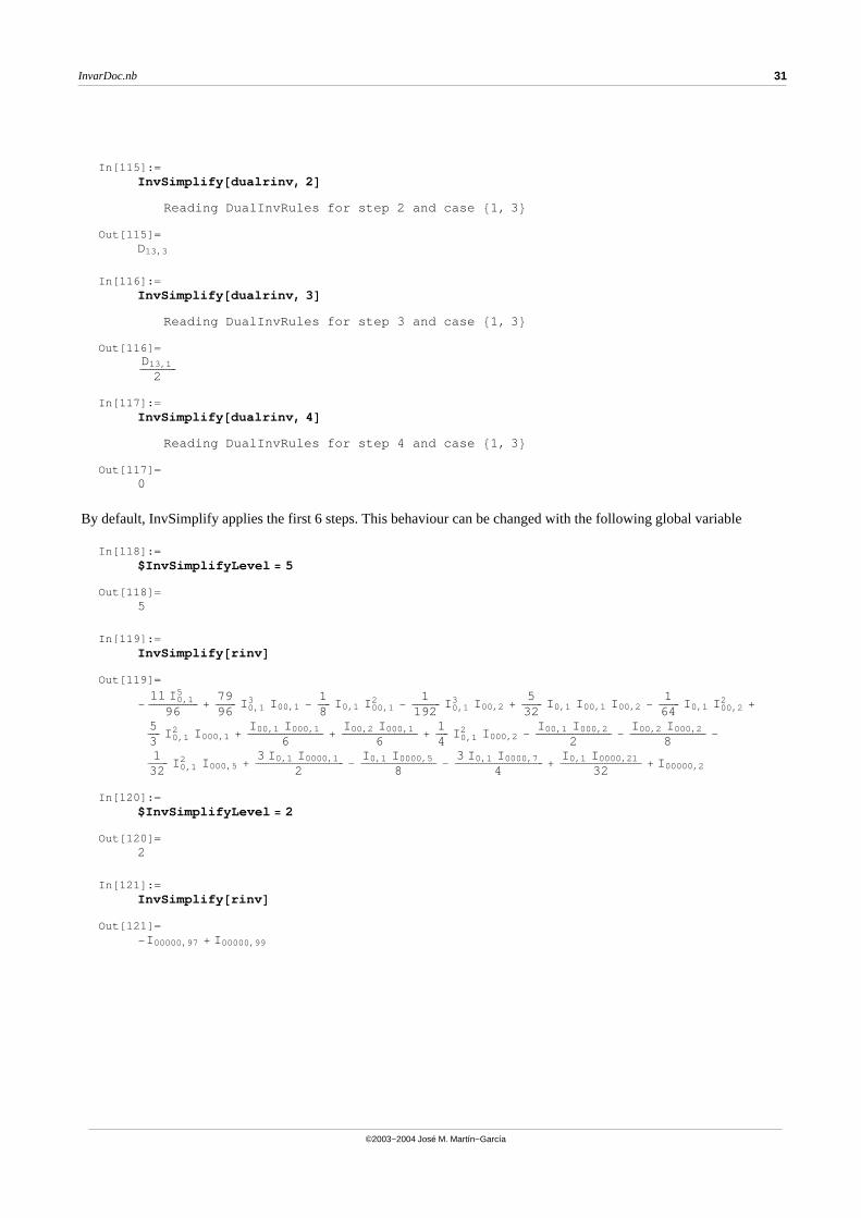
By default, InvSimplify applies the first 6 steps. This behaviour can be changed with the following global variable
In[118]:=$InvSimplifyLevel = 5
Out[118]=5
In[119]:=InvSimplify@rinvD
Out[119]=
-11 I 0,1
5
�������������������96
+79��������96
I 0,13 I 00,1 -
1�����8
I 0,1 I 00,12
-1
�����������192
I 0,13 I 00,2 +
5��������32
I 0,1 I 00,1 I 00,2 -1
��������64
I 0,1 I 00,22
+
5�����3
I 0,12 I 000,1 +
I 00,1 I 000,1�����������������������������
6+
I 00,2 I 000,1�����������������������������
6+
1�����4
I 0,12 I 000,2 -
I 00,1 I 000,2�����������������������������
2-
I 00,2 I 000,2�����������������������������
8-
1��������32
I 0,12 I 000,5 +
3 I 0,1 I 0000,1����������������������������������
2-
I 0,1 I 0000,5�����������������������������
8-
3 I 0,1 I 0000,7����������������������������������
4+
I 0,1 I 0000,21�������������������������������
32+ I 00000,2
In[120]:=$InvSimplifyLevel = 2
Out[120]=2
In[121]:=InvSimplify@rinvD
Out[121]=-I 00000,97 + I 00000,99
InvarDoc.nb 31
©2003−2004 José M. Martín−García
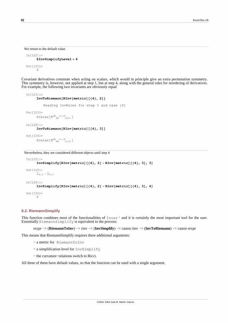
We return to the default value
In[122]:=$InvSimplifyLevel = 6
Out[122]=6
Covariant derivatives commute when acting on scalars, which would in principle give an extra permutation symmetry.This symmetry is, however, not applied at step 1, but at step 4, along with the general rules for reordering of derivatives.For example, the following two invariants are obviously equal
In[123]:=InvToRiemann@RInv@metricD@84<, 2DD
Reading InvRules for step 1 and case 84<Out[123]=
Scalar @R ab ;d;cab ;c ;d D
In[124]:=InvToRiemann@RInv@metricD@84<, 3DD
Out[124]=
Scalar @R ab ;c;dab ;c ;d D
Nevertheless, they are considered different objects until step 4
In[125]:=InvSimplify@RInv@metricD@84<, 2D - RInv@metricD@84<, 3D, 3D
Out[125]=I 4,2 - I 4,3
In[126]:=InvSimplify@RInv@metricD@84<, 2D - RInv@metricD@84<, 3D, 4D
Out[126]=0
6.2. RiemannSimplify
This function combines most of the functionalities of Invar‘ and it is certainly the most important tool for the user.Essentially RiemannSimplify is equivalent to the process:
rexpr −> (RiemannToInv) −> rinv −> (InvSimplify) −> canon rinv −> (InvToRiemann) −> canon rexpr
This means that RiemannSimplify requires three additional arguments:
− a metric for RiemannToInv
− a simplification level for InvSimplify
− the curvature−relations switch to Ricci.
All three of them have default values, so that the function can be used with a single argument.
32 InvarDoc.nb
©2003−2004 José M. Martín−García
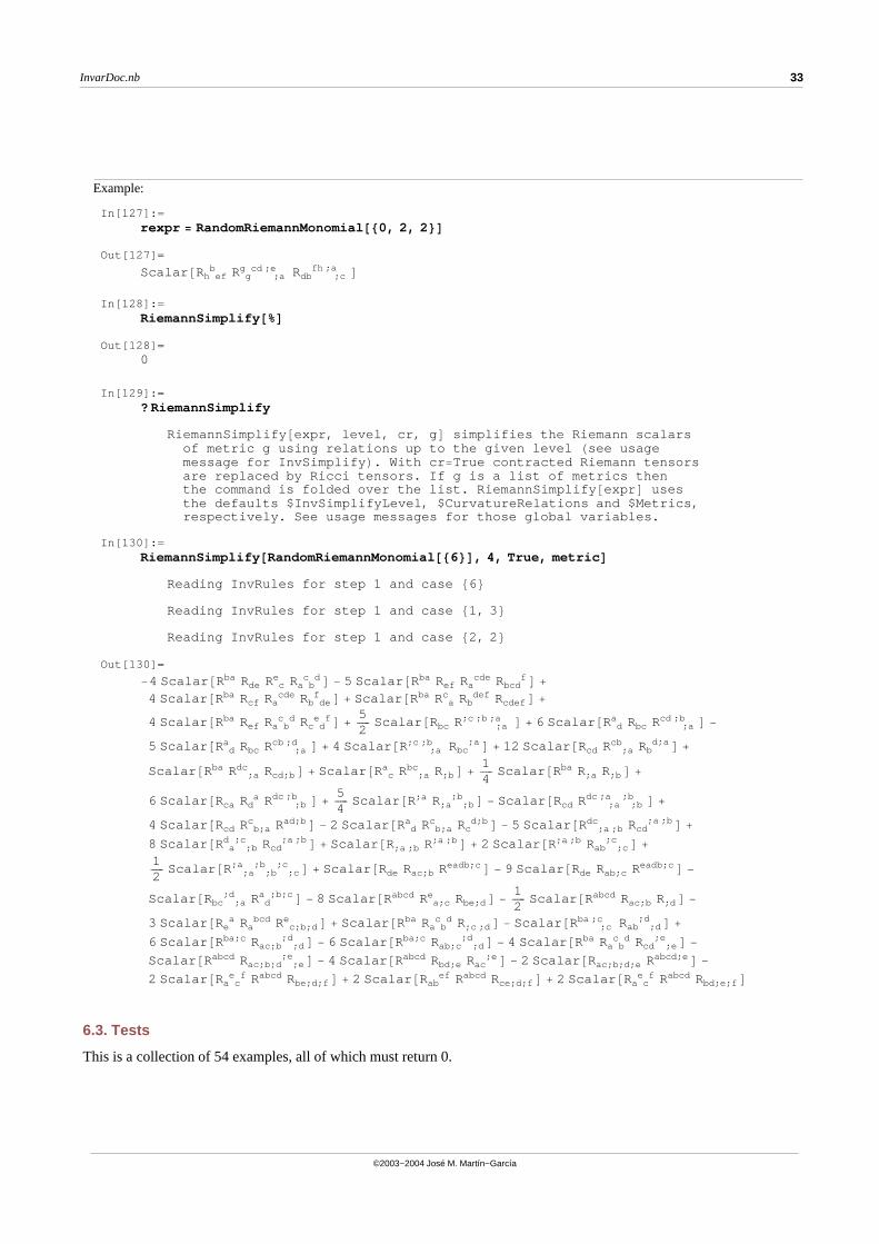
Example:
In[127]:=rexpr = RandomRiemannMonomial@80, 2, 2<D
Out[127]=
Scalar @Rh efb R g ;a
g cd ;e Rdb ;cfh ;a D
In[128]:=RiemannSimplify@%D
Out[128]=0
In[129]:=?RiemannSimplify
RiemannSimplify @expr, level, cr, g D simplifies the Riemann scalarsof metric g using relations up to the given level Hsee usagemessage for InvSimplify L. With cr =True contracted Riemann tensorsare replaced by Ricci tensors. If g is a list of metrics thenthe command is folded over the list. RiemannSimplify @expr D usesthe defaults $InvSimplifyLevel, $CurvatureRelations and $Metrics,respectively. See usage messages for those global variables.
In[130]:=RiemannSimplify@RandomRiemannMonomial@86<D, 4, True, metricD
Reading InvRules for step 1 and case 86<Reading InvRules for step 1 and case 81, 3 <Reading InvRules for step 1 and case 82, 2 <
Out[130]=
-4 Scalar @Rba Rde R ce Ra b
c d D - 5 Scalar @Rba Ref Racde Rbcd
f D +
4 Scalar @Rba Rcf Racde Rb de
f D + Scalar @Rba R ac Rb
def Rcdef D +
4 Scalar @Rba Ref Ra bc d Rc d
e f D +5�����2
Scalar @Rbc R ;a;c ;b ;a D + 6 Scalar @R d
a Rbc R ;acd ;b D -
5 Scalar @R da Rbc R ;a
cb ;d D + 4 Scalar @R ;a;c ;b Rbc
;a D + 12 Scalar @Rcd R ;acb Rb
d;a D +
Scalar @Rba R ;adc Rcd;b D + Scalar @R c
a R ;abc R;b D +
1�����4
Scalar @Rba R;a R;b D +
6 Scalar @Rca Rda R ;b
dc ;b D +5�����4
Scalar @R;a R;a ;b;b D - Scalar @Rcd R ;a ;b
dc ;a ;b D +
4 Scalar @Rcd R b;ac Rad;b D - 2 Scalar @R d
a R b;ac Rc
d;b D - 5 Scalar @R ;a ;bdc Rcd
;a ;b D +
8 Scalar @R a ;bd ;c Rcd
;a ;b D + Scalar @R;a ;b R;a ;b D + 2 Scalar @R;a ;b Rab ;c;c D +
1�����2
Scalar @R ;a ;b ;c;a ;b ;c D + Scalar @Rde Rac;b Readb;c D - 9 Scalar @Rde Rab;c Readb;c D -
Scalar @Rbc ;a;d R d
a ;b;c D - 8 Scalar @Rabcd R a;ce Rbe;d D -
1�����2
Scalar @Rabcd Rac;b R;d D -
3 Scalar @Rea Ra
bcd R c;b;de D + Scalar @Rba Ra b
c d R;c ;d D - Scalar @R ;cba ;c Rab ;d
;d D +
6 Scalar @Rba;c Rac;b ;d;d D - 6 Scalar @Rba;c Rab;c ;d
;d D - 4 Scalar @Rba Ra bc d Rcd ;e
;e D -
Scalar @Rabcd Rac;b;d ;e;e D - 4 Scalar @Rabcd Rbd;e Rac
;e D - 2 Scalar @Rac;b;d;e Rabcd;e D -
2 Scalar @Ra ce f Rabcd Rbe;d;f D + 2 Scalar @Rab
ef Rabcd Rce;d;f D + 2 Scalar @Ra ce f Rabcd Rbd;e;f D
6.3. Tests
This is a collection of 54 examples, all of which must return 0.
InvarDoc.nb 33
©2003−2004 José M. Martín−García
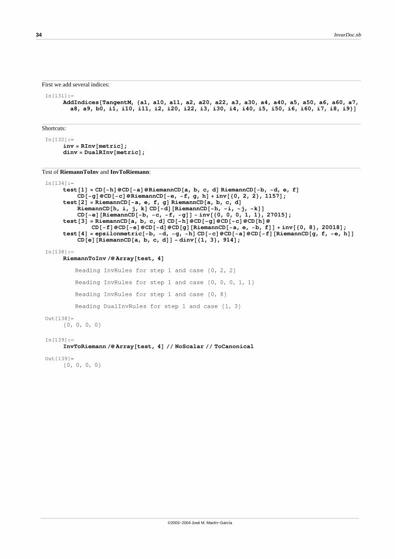
First we add several indices:
In[131]:=AddIndices@TangentM, 8a1, a10, a11, a2, a20, a22, a3, a30, a4, a40, a5, a50, a6, a60, a7,a8, a9, b0, i1, i10, i11, i2, i20, i22, i3, i30, i4, i40, i5, i50, i6, i60, i7, i8, i9<D
Shortcuts:
In[132]:=inv = RInv@metricD;dinv = DualRInv@metricD;
Test of RiemannToInv and InvToRiemann:
In[134]:=test@1D = CD@-hD�CD@-aD�RiemannCD@a, b, c, dD RiemannCD@-b, -d, e, fD
CD@-gD�CD@-cD�RiemannCD@-e, -f, g, hD + inv@80, 2, 2<, 1157D;test@2D = RiemannCD@-a, e, f, gD RiemannCD@a, b, c, dD
RiemannCD@h, i, j, kD CD@-dD@RiemannCD@-h, -i, -j, -kDD
CD@-eD@RiemannCD@-b, -c, -f, -gDD - inv@80, 0, 0, 1, 1<, 27015D;test@3D = RiemannCD@a, b, c, dD CD@-hD�CD@-gD�CD@-cD�CD@hD�
CD@-fD�CD@-eD�CD@-dD�CD@gD@RiemannCD@-a, e, -b, fDD + inv@80, 8<, 20018D;test@4D = epsilonmetric@-b, -d, -g, -hD CD@-cD�CD@-aD�CD@-fD@RiemannCD@g, f, -e, hDD
CD@eD@RiemannCD@a, b, c, dDD - dinv@81, 3<, 914D;
In[138]:=RiemannToInv �� Array@test, 4D
Reading InvRules for step 1 and case 80, 2, 2 <Reading InvRules for step 1 and case 80, 0, 0, 1, 1 <Reading InvRules for step 1 and case 80, 8 <Reading DualInvRules for step 1 and case 81, 3 <
Out[138]=80, 0, 0, 0 <
In[139]:=InvToRiemann �� Array@test, 4D �� NoScalar �� ToCanonical
Out[139]=80, 0, 0, 0 <
34 InvarDoc.nb
©2003−2004 José M. Martín−García
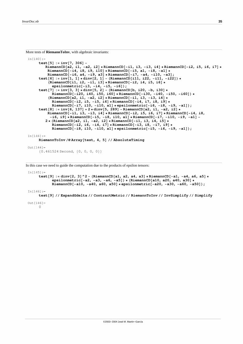
More tests of RiemannToInv, with algebraic invariants:
In[140]:=test@5D := inv@7, 306D -
RiemannCD@a2, i1, -a2, i2D*RiemannCD@-i1, i3, -i3, i4D*RiemannCD@-i2, i5, i6, i7D*
RiemannCD@-i4, i8, i9, i10D*RiemannCD@-i5, a1, -i8, -a1D*
RiemannCD@-i6, a4, -i9, a3D*RiemannCD@-i7, -a4, -i10, -a3D;test@6D := inv@1, 1D*dinv@2, 1D - HRiemannCD@i11, i22, -i11, -i22DL*
HRiemannCD@i1, i2, -i1, i3D*RiemannCD@-i2, i4, i5, i6D*
epsilonmetric@-i3, -i4, -i5, -i6DL;test@7D := inv@3, 3D*dinv@5, 2D - HRiemannCD@b, i20, -b, i30D*
RiemannCD@-i20, i40, i50, i60D*RiemannCD@-i30, -i40, -i50, -i60DL*
HRiemannCD@a2, i1, -a2, i2D*RiemannCD@-i1, i3, -i3, i4D*
RiemannCD@-i2, i5, -i5, i6D*RiemannCD@-i4, i7, i8, i9D*
RiemannCD@-i7, i10, -i10, a1D*epsilonmetric@-i6, -i8, -i9, -a1DL;test@8D := inv@6, 137D + 2*dinv@5, 289D - RiemannCD@a2, i1, -a2, i2D*
RiemannCD@-i1, i3, -i3, i4D*RiemannCD@-i2, i5, i6, i7D*RiemannCD@-i4, i8,-i6, i9D*RiemannCD@-i5, -i8, i10, a1D*RiemannCD@-i7, -i10, -i9, -a1D -
2*HRiemannCD@a2, i1, -a2, i2D*RiemannCD@-i1, i3, i4, i5D*
RiemannCD@-i2, i6, -i4, i7D*RiemannCD@-i3, i8, -i7, i9D*
RiemannCD@-i8, i10, -i10, a1D*epsilonmetric@-i5, -i6, -i9, -a1DL;
In[144]:=RiemannToInv �� Array@test, 4, 5D �� AbsoluteTiming
Out[144]=80.461524 Second, 80, 0, 0, 0 <<
In this case we need to guide the computation due to the products of epsilon tensors:
In[145]:=test@9D := dinv@2, 3D^2 - HRiemannCD@a1, a2, a4, a3D*RiemannCD@-a1, -a4, a6, a5D*
epsilonmetric@-a2, -a3, -a6, -a5DL*HRiemannCD@a10, a20, a40, a30D*
RiemannCD@-a10, -a40, a60, a50D*epsilonmetric@-a20, -a30, -a60, -a50DL;
In[146]:=test@9D �� ExpandGdelta �� ContractMetric �� RiemannToInv �� InvSimplify �� Simplify
Out[146]=0
InvarDoc.nb 35
©2003−2004 José M. Martín−García
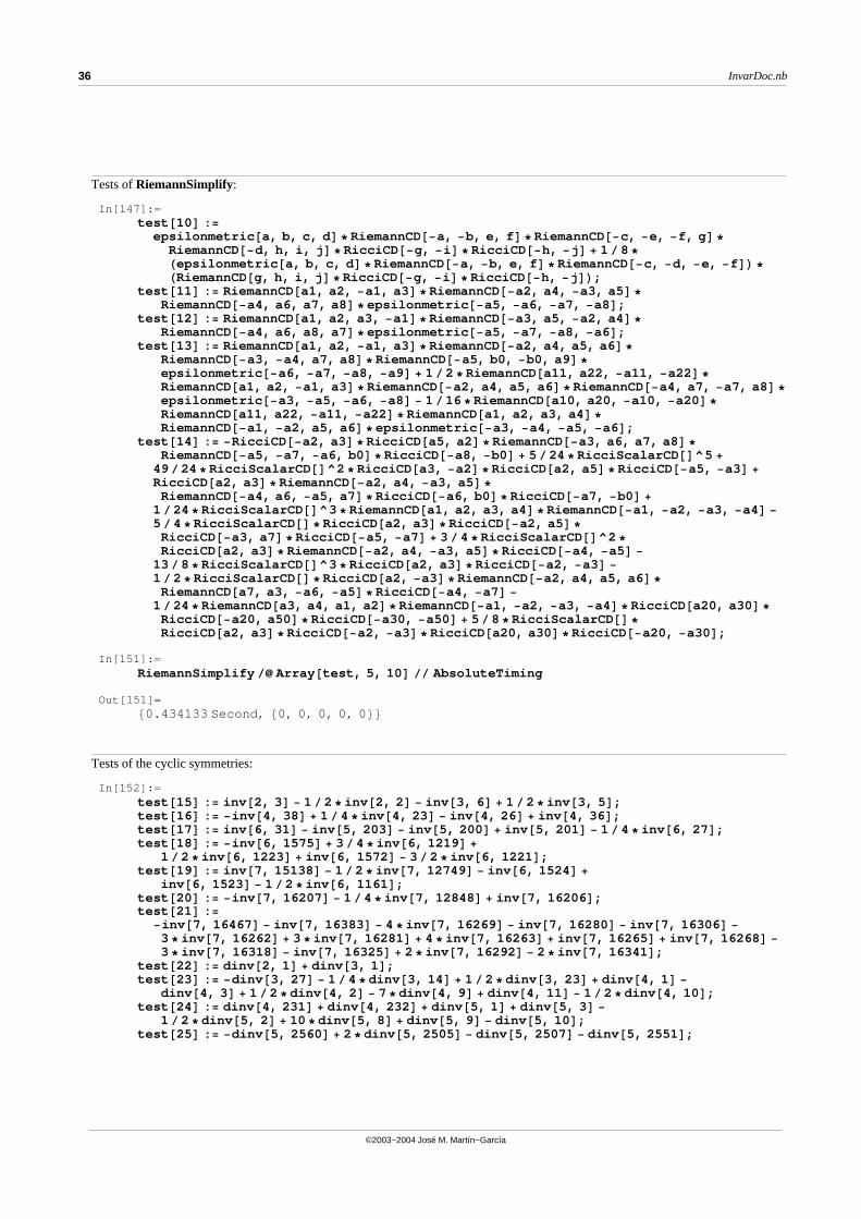
Tests of RiemannSimplify:
In[147]:=test@10D :=
epsilonmetric@a, b, c, dD*RiemannCD@-a, -b, e, fD*RiemannCD@-c, -e, -f, gD*
RiemannCD@-d, h, i, jD*RicciCD@-g, -iD*RicciCD@-h, -jD + 1�8*
Hepsilonmetric@a, b, c, dD*RiemannCD@-a, -b, e, fD*RiemannCD@-c, -d, -e, -fDL*
HRiemannCD@g, h, i, jD*RicciCD@-g, -iD*RicciCD@-h, -jDL;test@11D := RiemannCD@a1, a2, -a1, a3D*RiemannCD@-a2, a4, -a3, a5D*
RiemannCD@-a4, a6, a7, a8D*epsilonmetric@-a5, -a6, -a7, -a8D;test@12D := RiemannCD@a1, a2, a3, -a1D*RiemannCD@-a3, a5, -a2, a4D*
RiemannCD@-a4, a6, a8, a7D*epsilonmetric@-a5, -a7, -a8, -a6D;test@13D := RiemannCD@a1, a2, -a1, a3D*RiemannCD@-a2, a4, a5, a6D*
RiemannCD@-a3, -a4, a7, a8D*RiemannCD@-a5, b0, -b0, a9D*
epsilonmetric@-a6, -a7, -a8, -a9D + 1�2*RiemannCD@a11, a22, -a11, -a22D*
RiemannCD@a1, a2, -a1, a3D*RiemannCD@-a2, a4, a5, a6D*RiemannCD@-a4, a7, -a7, a8D*
epsilonmetric@-a3, -a5, -a6, -a8D - 1�16*RiemannCD@a10, a20, -a10, -a20D*
RiemannCD@a11, a22, -a11, -a22D*RiemannCD@a1, a2, a3, a4D*
RiemannCD@-a1, -a2, a5, a6D*epsilonmetric@-a3, -a4, -a5, -a6D;test@14D := -RicciCD@-a2, a3D*RicciCD@a5, a2D*RiemannCD@-a3, a6, a7, a8D*
RiemannCD@-a5, -a7, -a6, b0D*RicciCD@-a8, -b0D + 5�24*RicciScalarCD@D^5 +
49�24*RicciScalarCD@D^2*RicciCD@a3, -a2D*RicciCD@a2, a5D*RicciCD@-a5, -a3D +
RicciCD@a2, a3D*RiemannCD@-a2, a4, -a3, a5D*
RiemannCD@-a4, a6, -a5, a7D*RicciCD@-a6, b0D*RicciCD@-a7, -b0D +
1�24*RicciScalarCD@D^3*RiemannCD@a1, a2, a3, a4D*RiemannCD@-a1, -a2, -a3, -a4D -
5�4*RicciScalarCD@D*RicciCD@a2, a3D*RicciCD@-a2, a5D*
RicciCD@-a3, a7D*RicciCD@-a5, -a7D + 3�4*RicciScalarCD@D^2*
RicciCD@a2, a3D*RiemannCD@-a2, a4, -a3, a5D*RicciCD@-a4, -a5D -
13�8*RicciScalarCD@D^3*RicciCD@a2, a3D*RicciCD@-a2, -a3D -
1�2*RicciScalarCD@D*RicciCD@a2, -a3D*RiemannCD@-a2, a4, a5, a6D*
RiemannCD@a7, a3, -a6, -a5D*RicciCD@-a4, -a7D -
1�24*RiemannCD@a3, a4, a1, a2D*RiemannCD@-a1, -a2, -a3, -a4D*RicciCD@a20, a30D*
RicciCD@-a20, a50D*RicciCD@-a30, -a50D + 5�8*RicciScalarCD@D*
RicciCD@a2, a3D*RicciCD@-a2, -a3D*RicciCD@a20, a30D*RicciCD@-a20, -a30D;
In[151]:=RiemannSimplify �� Array@test, 5, 10D �� AbsoluteTiming
Out[151]=80.434133 Second, 80, 0, 0, 0, 0 <<
Tests of the cyclic symmetries:
In[152]:=test@15D := inv@2, 3D - 1�2*inv@2, 2D - inv@3, 6D + 1�2*inv@3, 5D;test@16D := -inv@4, 38D + 1�4*inv@4, 23D - inv@4, 26D + inv@4, 36D;test@17D := inv@6, 31D - inv@5, 203D - inv@5, 200D + inv@5, 201D - 1�4*inv@6, 27D;test@18D := -inv@6, 1575D + 3�4*inv@6, 1219D +
1�2*inv@6, 1223D + inv@6, 1572D - 3�2*inv@6, 1221D;test@19D := inv@7, 15138D - 1�2*inv@7, 12749D - inv@6, 1524D +
inv@6, 1523D - 1�2*inv@6, 1161D;test@20D := -inv@7, 16207D - 1�4*inv@7, 12848D + inv@7, 16206D;test@21D :=
-inv@7, 16467D - inv@7, 16383D - 4*inv@7, 16269D - inv@7, 16280D - inv@7, 16306D -
3*inv@7, 16262D + 3*inv@7, 16281D + 4*inv@7, 16263D + inv@7, 16265D + inv@7, 16268D -
3*inv@7, 16318D - inv@7, 16325D + 2*inv@7, 16292D - 2*inv@7, 16341D;test@22D := dinv@2, 1D + dinv@3, 1D;test@23D := -dinv@3, 27D - 1�4*dinv@3, 14D + 1�2*dinv@3, 23D + dinv@4, 1D -
dinv@4, 3D + 1�2*dinv@4, 2D - 7*dinv@4, 9D + dinv@4, 11D - 1�2*dinv@4, 10D;test@24D := dinv@4, 231D + dinv@4, 232D + dinv@5, 1D + dinv@5, 3D -
1�2*dinv@5, 2D + 10*dinv@5, 8D + dinv@5, 9D - dinv@5, 10D;test@25D := -dinv@5, 2560D + 2*dinv@5, 2505D - dinv@5, 2507D - dinv@5, 2551D;
36 InvarDoc.nb
©2003−2004 José M. Martín−García
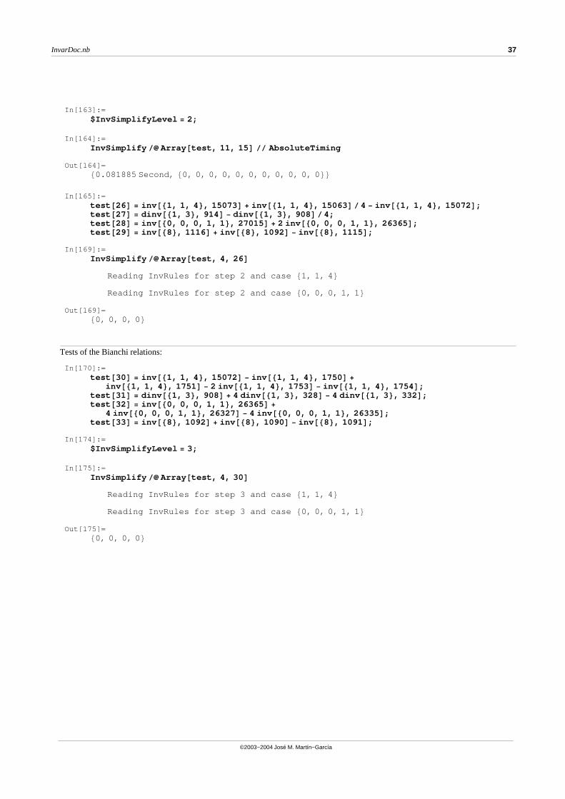
In[163]:=$InvSimplifyLevel = 2;
In[164]:=InvSimplify �� Array@test, 11, 15D �� AbsoluteTiming
Out[164]=80.081885 Second, 80, 0, 0, 0, 0, 0, 0, 0, 0, 0, 0 <<
In[165]:=test@26D = inv@81, 1, 4<, 15073D + inv@81, 1, 4<, 15063D�4 - inv@81, 1, 4<, 15072D;test@27D = dinv@81, 3<, 914D - dinv@81, 3<, 908D�4;test@28D = inv@80, 0, 0, 1, 1<, 27015D + 2 inv@80, 0, 0, 1, 1<, 26365D;test@29D = inv@88<, 1116D + inv@88<, 1092D - inv@88<, 1115D;
In[169]:=InvSimplify �� Array@test, 4, 26D
Reading InvRules for step 2 and case 81, 1, 4 <Reading InvRules for step 2 and case 80, 0, 0, 1, 1 <
Out[169]=80, 0, 0, 0 <
Tests of the Bianchi relations:
In[170]:=test@30D = inv@81, 1, 4<, 15072D - inv@81, 1, 4<, 1750D +
inv@81, 1, 4<, 1751D - 2 inv@81, 1, 4<, 1753D - inv@81, 1, 4<, 1754D;test@31D = dinv@81, 3<, 908D + 4 dinv@81, 3<, 328D - 4 dinv@81, 3<, 332D;test@32D = inv@80, 0, 0, 1, 1<, 26365D +
4 inv@80, 0, 0, 1, 1<, 26327D - 4 inv@80, 0, 0, 1, 1<, 26335D;test@33D = inv@88<, 1092D + inv@88<, 1090D - inv@88<, 1091D;
In[174]:=$InvSimplifyLevel = 3;
In[175]:=InvSimplify �� Array@test, 4, 30D
Reading InvRules for step 3 and case 81, 1, 4 <Reading InvRules for step 3 and case 80, 0, 0, 1, 1 <
Out[175]=80, 0, 0, 0 <
InvarDoc.nb 37
©2003−2004 José M. Martín−García
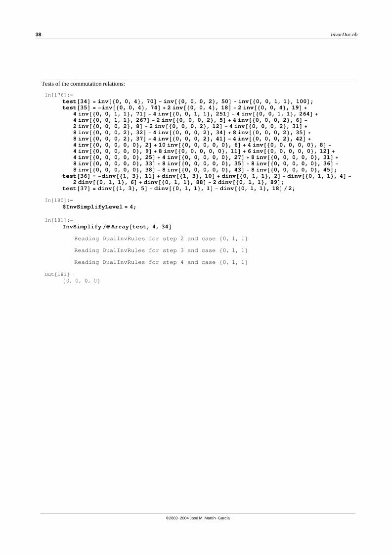
Tests of the commutation relations:
In[176]:=test@34D = inv@80, 0, 4<, 70D - inv@80, 0, 0, 2<, 50D - inv@80, 0, 1, 1<, 100D;test@35D = -inv@80, 0, 4<, 74D + 2 inv@80, 0, 4<, 18D - 2 inv@80, 0, 4<, 19D +
4 inv@80, 0, 1, 1<, 71D - 4 inv@80, 0, 1, 1<, 251D - 4 inv@80, 0, 1, 1<, 264D +
4 inv@80, 0, 1, 1<, 267D - 2 inv@80, 0, 0, 2<, 5D + 4 inv@80, 0, 0, 2<, 6D -
2 inv@80, 0, 0, 2<, 8D - 2 inv@80, 0, 0, 2<, 12D - 4 inv@80, 0, 0, 2<, 31D +
8 inv@80, 0, 0, 2<, 32D - 4 inv@80, 0, 0, 2<, 34D + 8 inv@80, 0, 0, 2<, 35D +
8 inv@80, 0, 0, 2<, 37D - 4 inv@80, 0, 0, 2<, 41D - 4 inv@80, 0, 0, 2<, 42D +
4 inv@80, 0, 0, 0, 0<, 2D + 10 inv@80, 0, 0, 0, 0<, 6D + 4 inv@80, 0, 0, 0, 0<, 8D -
4 inv@80, 0, 0, 0, 0<, 9D + 8 inv@80, 0, 0, 0, 0<, 11D + 6 inv@80, 0, 0, 0, 0<, 12D +
4 inv@80, 0, 0, 0, 0<, 25D + 4 inv@80, 0, 0, 0, 0<, 27D + 8 inv@80, 0, 0, 0, 0<, 31D +
8 inv@80, 0, 0, 0, 0<, 33D + 8 inv@80, 0, 0, 0, 0<, 35D - 8 inv@80, 0, 0, 0, 0<, 36D -
8 inv@80, 0, 0, 0, 0<, 38D - 8 inv@80, 0, 0, 0, 0<, 43D - 8 inv@80, 0, 0, 0, 0<, 45D;test@36D = -dinv@81, 3<, 11D + dinv@81, 3<, 10D + dinv@80, 1, 1<, 2D - dinv@80, 1, 1<, 4D -
2 dinv@80, 1, 1<, 6D + dinv@80, 1, 1<, 88D - 2 dinv@80, 1, 1<, 89D;test@37D = dinv@81, 3<, 5D - dinv@80, 1, 1<, 1D - dinv@80, 1, 1<, 18D�2;
In[180]:=$InvSimplifyLevel = 4;
In[181]:=InvSimplify �� Array@test, 4, 34D
Reading DualInvRules for step 2 and case 80, 1, 1 <Reading DualInvRules for step 3 and case 80, 1, 1 <Reading DualInvRules for step 4 and case 80, 1, 1 <
Out[181]=80, 0, 0, 0 <
38 InvarDoc.nb
©2003−2004 José M. Martín−García
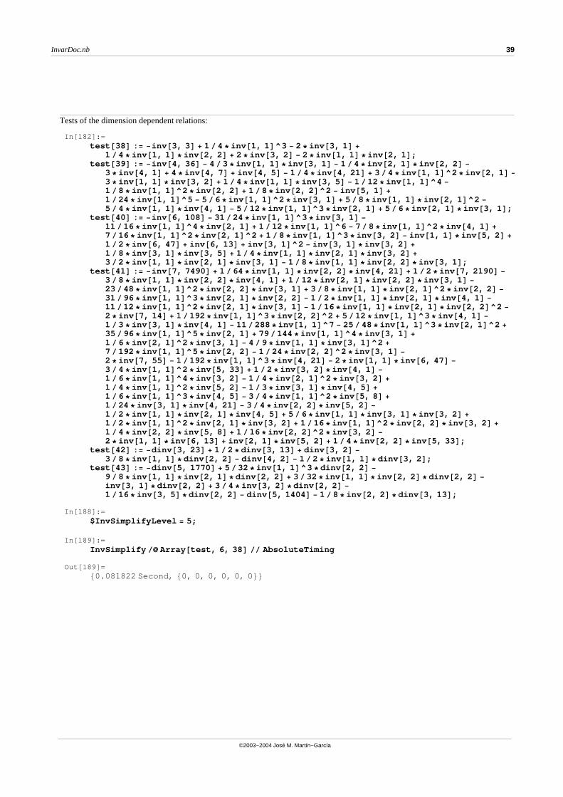
Tests of the dimension dependent relations:
In[182]:=test@38D := -inv@3, 3D + 1�4*inv@1, 1D^3 - 2*inv@3, 1D +
1�4*inv@1, 1D*inv@2, 2D + 2*inv@3, 2D - 2*inv@1, 1D*inv@2, 1D;test@39D := -inv@4, 36D - 4�3*inv@1, 1D*inv@3, 1D - 1�4*inv@2, 1D*inv@2, 2D -
3*inv@4, 1D + 4*inv@4, 7D + inv@4, 5D - 1�4*inv@4, 21D + 3�4*inv@1, 1D^2*inv@2, 1D -
3*inv@1, 1D*inv@3, 2D + 1�4*inv@1, 1D*inv@3, 5D - 1�12*inv@1, 1D^4 -
1�8*inv@1, 1D^2*inv@2, 2D + 1�8*inv@2, 2D^2 - inv@5, 1D +
1�24*inv@1, 1D^5 - 5�6*inv@1, 1D^2*inv@3, 1D + 5�8*inv@1, 1D*inv@2, 1D^2 -
5�4*inv@1, 1D*inv@4, 1D - 5�12*inv@1, 1D^3*inv@2, 1D + 5�6*inv@2, 1D*inv@3, 1D;test@40D := -inv@6, 108D - 31�24*inv@1, 1D^3*inv@3, 1D -
11�16*inv@1, 1D^4*inv@2, 1D + 1�12*inv@1, 1D^6 - 7�8*inv@1, 1D^2*inv@4, 1D +
7�16*inv@1, 1D^2*inv@2, 1D^2 + 1�8*inv@1, 1D^3*inv@3, 2D - inv@1, 1D*inv@5, 2D +
1�2*inv@6, 47D + inv@6, 13D + inv@3, 1D^2 - inv@3, 1D*inv@3, 2D +
1�8*inv@3, 1D*inv@3, 5D + 1�4*inv@1, 1D*inv@2, 1D*inv@3, 2D +
3�2*inv@1, 1D*inv@2, 1D*inv@3, 1D - 1�8*inv@1, 1D*inv@2, 2D*inv@3, 1D;test@41D := -inv@7, 7490D + 1�64*inv@1, 1D*inv@2, 2D*inv@4, 21D + 1�2*inv@7, 2190D -
3�8*inv@1, 1D*inv@2, 2D*inv@4, 1D + 1�12*inv@2, 1D*inv@2, 2D*inv@3, 1D -
23�48*inv@1, 1D^2*inv@2, 2D*inv@3, 1D + 3�8*inv@1, 1D*inv@2, 1D^2*inv@2, 2D -
31�96*inv@1, 1D^3*inv@2, 1D*inv@2, 2D - 1�2*inv@1, 1D*inv@2, 1D*inv@4, 1D -
11�12*inv@1, 1D^2*inv@2, 1D*inv@3, 1D - 1�16*inv@1, 1D*inv@2, 1D*inv@2, 2D^2 -
2*inv@7, 14D + 1�192*inv@1, 1D^3*inv@2, 2D^2 + 5�12*inv@1, 1D^3*inv@4, 1D -
1�3*inv@3, 1D*inv@4, 1D - 11�288*inv@1, 1D^7 - 25�48*inv@1, 1D^3*inv@2, 1D^2 +
35�96*inv@1, 1D^5*inv@2, 1D + 79�144*inv@1, 1D^4*inv@3, 1D +
1�6*inv@2, 1D^2*inv@3, 1D - 4�9*inv@1, 1D*inv@3, 1D^2 +
7�192*inv@1, 1D^5*inv@2, 2D - 1�24*inv@2, 2D^2*inv@3, 1D -
2*inv@7, 55D - 1�192*inv@1, 1D^3*inv@4, 21D - 2*inv@1, 1D*inv@6, 47D -
3�4*inv@1, 1D^2*inv@5, 33D + 1�2*inv@3, 2D*inv@4, 1D -
1�6*inv@1, 1D^4*inv@3, 2D - 1�4*inv@2, 1D^2*inv@3, 2D +
1�4*inv@1, 1D^2*inv@5, 2D - 1�3*inv@3, 1D*inv@4, 5D +
1�6*inv@1, 1D^3*inv@4, 5D - 3�4*inv@1, 1D^2*inv@5, 8D +
1�24*inv@3, 1D*inv@4, 21D - 3�4*inv@2, 2D*inv@5, 2D -
1�2*inv@1, 1D*inv@2, 1D*inv@4, 5D + 5�6*inv@1, 1D*inv@3, 1D*inv@3, 2D +
1�2*inv@1, 1D^2*inv@2, 1D*inv@3, 2D + 1�16*inv@1, 1D^2*inv@2, 2D*inv@3, 2D +
1�4*inv@2, 2D*inv@5, 8D + 1�16*inv@2, 2D^2*inv@3, 2D -
2*inv@1, 1D*inv@6, 13D + inv@2, 1D*inv@5, 2D + 1�4*inv@2, 2D*inv@5, 33D;test@42D := -dinv@3, 23D + 1�2*dinv@3, 13D + dinv@3, 2D -
3�8*inv@1, 1D*dinv@2, 2D - dinv@4, 2D - 1�2*inv@1, 1D*dinv@3, 2D;test@43D := -dinv@5, 1770D + 5�32*inv@1, 1D^3*dinv@2, 2D -
9�8*inv@1, 1D*inv@2, 1D*dinv@2, 2D + 3�32*inv@1, 1D*inv@2, 2D*dinv@2, 2D -
inv@3, 1D*dinv@2, 2D + 3�4*inv@3, 2D*dinv@2, 2D -
1�16*inv@3, 5D*dinv@2, 2D - dinv@5, 1404D - 1�8*inv@2, 2D*dinv@3, 13D;
In[188]:=$InvSimplifyLevel = 5;
In[189]:=InvSimplify �� Array@test, 6, 38D �� AbsoluteTiming
Out[189]=80.081822 Second, 80, 0, 0, 0, 0, 0 <<
InvarDoc.nb 39
©2003−2004 José M. Martín−García
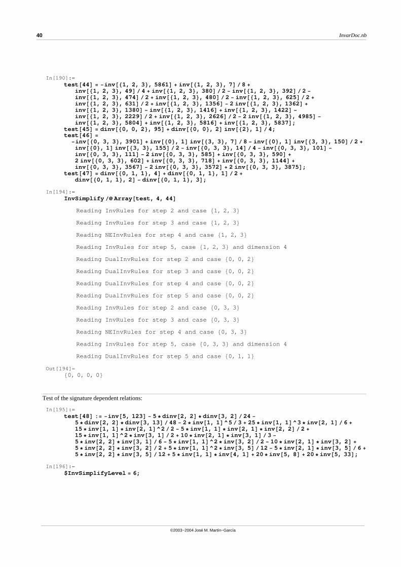
In[190]:=test@44D = -inv@81, 2, 3<, 5861D + inv@81, 2, 3<, 7D�8 +
inv@81, 2, 3<, 49D�4 + inv@81, 2, 3<, 380D�2 - inv@81, 2, 3<, 392D�2 -
inv@81, 2, 3<, 474D�2 + inv@81, 2, 3<, 480D�2 - inv@81, 2, 3<, 625D�2 +
inv@81, 2, 3<, 631D�2 + inv@81, 2, 3<, 1356D - 2 inv@81, 2, 3<, 1362D +
inv@81, 2, 3<, 1380D - inv@81, 2, 3<, 1416D + inv@81, 2, 3<, 1422D -
inv@81, 2, 3<, 2229D�2 + inv@81, 2, 3<, 2626D�2 - 2 inv@81, 2, 3<, 4985D -
inv@81, 2, 3<, 5804D + inv@81, 2, 3<, 5816D + inv@81, 2, 3<, 5837D;test@45D = dinv@80, 0, 2<, 95D + dinv@80, 0<, 2D inv@82<, 1D�4;test@46D =
-inv@80, 3, 3<, 3901D + inv@80<, 1D inv@83, 3<, 7D�8 - inv@80<, 1D inv@83, 3<, 150D�2 +
inv@80<, 1D inv@83, 3<, 155D�2 - inv@80, 3, 3<, 14D�4 - inv@80, 3, 3<, 101D -
inv@80, 3, 3<, 111D - 2 inv@80, 3, 3<, 585D + inv@80, 3, 3<, 590D +
2 inv@80, 3, 3<, 602D + inv@80, 3, 3<, 718D + inv@80, 3, 3<, 1144D +
inv@80, 3, 3<, 3567D - 2 inv@80, 3, 3<, 3572D + 2 inv@80, 3, 3<, 3875D;test@47D = dinv@80, 1, 1<, 4D + dinv@80, 1, 1<, 1D�2 +
dinv@80, 1, 1<, 2D - dinv@80, 1, 1<, 3D;
In[194]:=InvSimplify �� Array@test, 4, 44D
Reading InvRules for step 2 and case 81, 2, 3 <Reading InvRules for step 3 and case 81, 2, 3 <Reading NEInvRules for step 4 and case 81, 2, 3 <Reading InvRules for step 5, case 81, 2, 3 < and dimension 4
Reading DualInvRules for step 2 and case 80, 0, 2 <Reading DualInvRules for step 3 and case 80, 0, 2 <Reading DualInvRules for step 4 and case 80, 0, 2 <Reading DualInvRules for step 5 and case 80, 0, 2 <Reading InvRules for step 2 and case 80, 3, 3 <Reading InvRules for step 3 and case 80, 3, 3 <Reading NEInvRules for step 4 and case 80, 3, 3 <Reading InvRules for step 5, case 80, 3, 3 < and dimension 4
Reading DualInvRules for step 5 and case 80, 1, 1 <Out[194]=
80, 0, 0, 0 <
Test of the signature dependent relations:
In[195]:=test@48D := -inv@5, 123D - 5*dinv@2, 2D*dinv@3, 2D�24 -
5*dinv@2, 2D*dinv@3, 13D�48 - 2*inv@1, 1D^5�3 + 25*inv@1, 1D^3*inv@2, 1D�6 +
15*inv@1, 1D*inv@2, 1D^2�2 - 5*inv@1, 1D*inv@2, 1D*inv@2, 2D�2 +
15*inv@1, 1D^2*inv@3, 1D�2 + 10*inv@2, 1D*inv@3, 1D�3 -
5*inv@2, 2D*inv@3, 1D�6 - 5*inv@1, 1D^2*inv@3, 2D�2 - 10*inv@2, 1D*inv@3, 2D +
5*inv@2, 2D*inv@3, 2D�2 + 5*inv@1, 1D^2*inv@3, 5D�12 - 5*inv@2, 1D*inv@3, 5D�6 +
5*inv@2, 2D*inv@3, 5D�12 + 5*inv@1, 1D*inv@4, 1D + 20*inv@5, 8D + 20*inv@5, 33D;
In[196]:=$InvSimplifyLevel = 6;
40 InvarDoc.nb
©2003−2004 José M. Martín−García
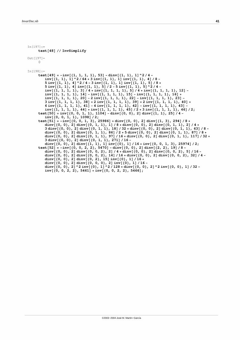
In[197]:=test@48D �� InvSimplify
Out[197]=0
In[198]:=test@49D = -inv@81, 1, 1, 1<, 53D - dinv@81, 1<, 1D^2�4 -
inv@81, 1<, 1D^2�64 + 3 inv@81, 1<, 1D inv@81, 1<, 4D�8 -
5 inv@81, 1<, 4D^2�4 - 3 inv@81, 1<, 1D inv@81, 1<, 5D�8 +
5 inv@81, 1<, 4D inv@81, 1<, 5D�2 - 5 inv@81, 1<, 5D^2�4 -
inv@81, 1, 1, 1<, 3D�4 + inv@81, 1, 1, 1<, 5D�4 + inv@81, 1, 1, 1<, 12D -
inv@81, 1, 1, 1<, 14D - inv@81, 1, 1, 1<, 15D - inv@81, 1, 1, 1<, 16D +
inv@81, 1, 1, 1<, 20D - 2 inv@81, 1, 1, 1<, 22D - inv@81, 1, 1, 1<, 23D -
3 inv@81, 1, 1, 1<, 38D + 2 inv@81, 1, 1, 1<, 39D + 2 inv@81, 1, 1, 1<, 40D +
6 inv@81, 1, 1, 1<, 41D - 4 inv@81, 1, 1, 1<, 42D - inv@81, 1, 1, 1<, 43D -
inv@81, 1, 1, 1<, 44D + inv@81, 1, 1, 1<, 45D�2 + 3 inv@81, 1, 1, 1<, 46D�2;test@50D = inv@80, 0, 1, 1<, 1104D - dinv@80, 0<, 2D dinv@81, 1<, 25D�4 -
inv@80, 0, 1, 1<, 1098D�2;test@51D = -inv@80, 0, 1, 3<, 25986D + dinv@80, 0<, 2D dinv@81, 3<, 294D�8 +
dinv@80, 0<, 2D dinv@80, 1, 1<, 1D�8 + dinv@80, 0<, 2D dinv@80, 1, 1<, 2D�4 +
3 dinv@80, 0<, 2D dinv@80, 1, 1<, 18D�32 + dinv@80, 0<, 2D dinv@80, 1, 1<, 63D�8 -
dinv@80, 0<, 2D dinv@80, 1, 1<, 86D�2 + 5 dinv@80, 0<, 2D dinv@80, 1, 1<, 87D�8 +
dinv@80, 0<, 2D dinv@80, 1, 1<, 97D�16 + dinv@80, 0<, 2D dinv@80, 1, 1<, 117D�32 +
3 dinv@80, 0<, 2D dinv@80, 1, 1<, 271D�16 -
dinv@80, 0<, 2D dinv@81, 1<, 1D inv@80<, 1D�16 + inv@80, 0, 1, 3<, 25974D�2;test@52D = -inv@80, 0, 2, 2<, 5470D - dinv@80, 0<, 2D dinv@82, 2<, 19D�8 -
dinv@80, 0<, 2D dinv@80, 0, 2<, 2D�4 + dinv@80, 0<, 2D dinv@80, 0, 2<, 5D�16 -
dinv@80, 0<, 2D dinv@80, 0, 2<, 14D�16 + dinv@80, 0<, 2D dinv@80, 0, 2<, 32D�4 -
dinv@80, 0<, 2D dinv@80, 2<, 15D inv@80<, 1D�16 +
dinv@80, 0<, 2D dinv@80, 0, 0<, 2D inv@80<, 1D�16 -
dinv@80, 0<, 2D^2 inv@80<, 1D^2�128 + dinv@80, 0<, 2D^2 inv@80, 0<, 1D�32 -
inv@80, 0, 2, 2<, 5461D + inv@80, 0, 2, 2<, 5466D;
InvarDoc.nb 41
©2003−2004 José M. Martín−García
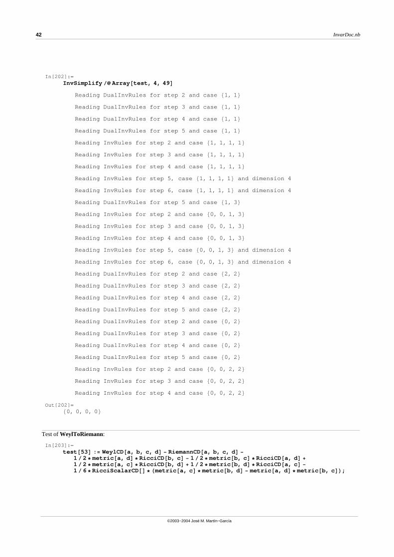
In[202]:=InvSimplify �� Array@test, 4, 49D
Reading DualInvRules for step 2 and case 81, 1 <Reading DualInvRules for step 3 and case 81, 1 <Reading DualInvRules for step 4 and case 81, 1 <Reading DualInvRules for step 5 and case 81, 1 <Reading InvRules for step 2 and case 81, 1, 1, 1 <Reading InvRules for step 3 and case 81, 1, 1, 1 <Reading InvRules for step 4 and case 81, 1, 1, 1 <Reading InvRules for step 5, case 81, 1, 1, 1 < and dimension 4
Reading InvRules for step 6, case 81, 1, 1, 1 < and dimension 4
Reading DualInvRules for step 5 and case 81, 3 <Reading InvRules for step 2 and case 80, 0, 1, 3 <Reading InvRules for step 3 and case 80, 0, 1, 3 <Reading InvRules for step 4 and case 80, 0, 1, 3 <Reading InvRules for step 5, case 80, 0, 1, 3 < and dimension 4
Reading InvRules for step 6, case 80, 0, 1, 3 < and dimension 4
Reading DualInvRules for step 2 and case 82, 2 <Reading DualInvRules for step 3 and case 82, 2 <Reading DualInvRules for step 4 and case 82, 2 <Reading DualInvRules for step 5 and case 82, 2 <Reading DualInvRules for step 2 and case 80, 2 <Reading DualInvRules for step 3 and case 80, 2 <Reading DualInvRules for step 4 and case 80, 2 <Reading DualInvRules for step 5 and case 80, 2 <Reading InvRules for step 2 and case 80, 0, 2, 2 <Reading InvRules for step 3 and case 80, 0, 2, 2 <Reading InvRules for step 4 and case 80, 0, 2, 2 <
Out[202]=80, 0, 0, 0 <
Test of WeylToRiemann:
In[203]:=test@53D := WeylCD@a, b, c, dD - RiemannCD@a, b, c, dD -
1�2* metric@a, dD*RicciCD@b, cD - 1�2* metric@b, cD*RicciCD@a, dD +
1�2* metric@a, cD*RicciCD@b, dD + 1�2* metric@b, dD*RicciCD@a, cD -
1�6*RicciScalarCD@D*Hmetric@a, cD* metric@b, dD - metric@a, dD* metric@b, cDL;
42 InvarDoc.nb
©2003−2004 José M. Martín−García
In[204]:=test@53D �� WeylToRiemann �� Simplify �� AbsoluteTiming
Out[204]=80.027630 Second, 0 <
Test of ContractCurvature:
In[205]:=test@54D := RiemannCD@c, d, -c, -dD*
RiemannCD@a, f, b, -fD*RiemannCD@-a, -b, h, lD* metric@-h, -lD -
RicciScalarCD@D*RicciCD@a, bD*RiemannCD@-a, -b, h, lD* metric@-h, -lD;
In[206]:=test@54D �� ContractCurvature �� ContractMetric �� AbsoluteTiming
Out[206]=80.004365 Second, 0 <
Tidy up:
In[207]:=RemoveIndices@TangentM,8a1, a10, a11, a2, a20, a22, a3, a30, a4, a40, a5, a50, a6, a60, a7, a8, a9, b0,i1, i10, i11, i2, i20, i22, i3, i30, i4, i40, i5, i50, i6, i60, i7, i8, i9<D;
Remove@testD
6.4. Zero powers of Riemann
Surprisingly, there are monomials of the Riemann tensor which are zero due to the cyclic symmetry only. This firsthappens for a single monomial of degree 6:
It does not happen for degrees 1 to 5:
In[209]:=Cases@RInvRules@2, 1D, HoldPattern@_ ® 0DD
Out[209]=8<
In[210]:=Cases@RInvRules@2, 2D, HoldPattern@_ ® 0DD
Out[210]=8<
In[211]:=Cases@RInvRules@2, 3D, HoldPattern@_ ® 0DD
Out[211]=8<
In[212]:=Cases@RInvRules@2, 4D, HoldPattern@_ ® 0DD
Out[212]=8<
InvarDoc.nb 43
©2003−2004 José M. Martín−García
In[213]:=Cases@RInvRules@2, 5D, HoldPattern@_ ® 0DD
Out[213]=8<
There is a single case in degree 6:
In[214]:=Cases@RInvRules@2, 6D, HoldPattern@_ ® 0DD
Out[214]=8I 000000,1461 ® 0<
And 19 more cases for degree 7:
In[215]:=Cases@RInvRules@2, 7D, HoldPattern@_ ® 0DD
Out[215]=8I 0000000,663 ® 0, I 0000000,1600 ® 0, I 0000000,1601 ® 0, I 0000000,3439 ® 0, I 0000000,3440 ® 0,
I 0000000,3460 ® 0, I 0000000,4987 ® 0, I 0000000,4988 ® 0, I 0000000,5822 ® 0, I 0000000,6830 ® 0,I 0000000,6831 ® 0, I 0000000,7545 ® 0, I 0000000,7546 ® 0, I 0000000,10851 ® 0, I 0000000,10852 ® 0,I 0000000,11644 ® 0, I 0000000,13382 ® 0, I 0000000,13843 ® 0, I 0000000,14054 ® 0<
There is no obvious reason why this should be zero, and for all dimensions:
In[216]:=RInv@metricD@6, 1461D �� InvToRiemann �� NoScalar
Out[216]=
Racef Rabcd Rb
ghi Rd hj k Reij
l Rfkgl
but we can check it in the pure Ricci case:
In[217]:=expr =
% �. RiemannCD@a_, b_, c_, d_D ® RicciCD@a, cD delta@b, dD + delta@a, cD RicciCD@b, dD -
RicciCD@a, dD delta@b, cD - delta@a, dD RicciCD@b, cD
Out[217]=
Hgbd Rac- gbc Rad
- gad Rbc+ gac Rbd L H∆c
f Rae
- ∆ce Ra
f- ∆a
f Rce
+ ∆ae Rc
f LHggi Rb
h- ggh Rb
i- ∆b
i Rgh+ ∆b
h Rgi L H∆il Rej - gij Re
l- ∆e
l Rij + gej Ril L
Hgjk Rdh - ∆ hj Rd
k- ∆d
k R hj
+ gdh Rjk L Hgkl Rfg - gkg Rfl - gfl Rkg + gfg Rkl L
In[218]:=expr@@1DD expr@@2DD �� ContractMetric �� ToCanonical
Out[218]=
-2 Rad Rbc+ 2 Rac Rbd
+ gce Rba R ad
- gbe Rca R ad
- gcd Rba R ae
+ gbd Rca R ae
44 InvarDoc.nb
©2003−2004 José M. Martín−García
In[219]:=% expr@@3DD �� ContractMetric �� ToCanonical
Out[219]=
geg Rba Rcf R ad
- gef Rba Rcg R ad
- 2 Rac Rbf Rde+ 2 Rab Rcf Rde
+ 2 Rac Rbe Rdf-
geg Rba R ac Rdf
- 2 Rab Rce Rdf+ gef Rba R a
c Rdg+ gdg Rba R a
c Ref- gcg Rba R a
d Ref-
gdf Rba R ac Reg
+ gcf Rba R ad Reg
+ 2 geg Rbd Rca R af
- 2 geg Rbc Rda R af
+ gbd Rca Reg R af
-
gbc Rda Reg R af
- 2 gef Rbd Rca R ag
+ 2 gef Rbc Rda R ag
- gbd Rca Ref R ag
+ gbc Rda Ref R ag
+
gce gfh Rab Rda Rgb- gcd gfh Rab Rea Rgb
- gce gfg Rab Rda Rhb+ gcd gfg Rab Rea Rhb
In[220]:=% expr@@4DD �� ContractMetric �� ToCanonical
Out[220]=
3 Rbg Rca R fd R a
e- 3 R f
b Rca Rdg R ae
+ 2 Rba R ac Rdg R f
e- 2 Rba R a
c R fd Reg
+ 2 Rbg Rce Rda Rfa -
3 Rbg Rca Rde Rfa + 3 Rba Rcg Rde Rfa - 3 Rba Rce Rdg Rfa + 4 Rbc Rdg Rea Rfa - 2 Rbc Rda Reg Rfa -
geh Rab R gc Rda Rfb
+ ∆ ge Rab Rch Rda Rfb
+ gch Rab Rda R ge Rfb
- ∆ gc Rab Rda Reh Rfb
-
2 geh Rca Rdb R bf Rga - gfh Rca R a
d Reb Rgb + gch Rda Reb R af Rgb + geh Rca R a
d Rfb Rgb -
3 gef Rab Rch Rda Rgb
- geh Rab Rca Rdf Rgb
+ gef Rab Rca Rdh Rgb
+ gdh Rab Rca Ref Rgb
-
gch Rab Rda Ref Rgb
- gdf Rab Rca Reh Rgb
+ 2 geh Rab Rcd Rfa Rgb
+ 2 gcd Rab Reh Rfa Rgb
-
2 R fb Rce Rda R a
g+ 3 R f
b Rca Rde R ag
- 3 Rba R fc Rde R a
g+ 3 Rba Rce R f
d R ag
-
4 Rbc R fd Rea R a
g+ 2 Rbc Rda R f
e R ag
- gci gfg Rad Rbd Rea Rh
b+ gce gfi Ra
d Rbd Rga Rhb
+
2 ∆ ge Rca Rdb R b
f R ah
- 3 gef Rca Rdb Rgb R ah
+ gdf Rca Reb Rgb R ah
+ gcd Rea Rfb Rgb R ah
+
∆ gf Rca R a
d Reb R bh
- ∆ gc Rda Reb R a
f R bh
- ∆ ge Rca R a
d Rfb R bh
+ 3 gef Rca Rdb Rga R bh
-
gdf Rca Reb Rga R bh
- gcd Rea Rfb Rga R bh
+ 3 gef Rab R gc Rda Rhb
+ ∆ ge Rab Rca Rdf Rhb
-
gef Rab Rca R gd Rhb
- ∆ gd Rab Rca Ref Rhb
+ ∆ gc Rab Rda Ref Rhb
+ gdf Rab Rca R ge Rhb
-
2 ∆ ge Rab Rcd Rfa Rhb
- 2 gcd Rab R ge Rfa Rhb
+ ∆ hc gfg Ra
d Rbd Rea Rib- ∆ h
f gce Rad Rbd Rga Rib
In[221]:=% expr@@5DD �� ContractMetric �� ToCanonical
Out[221]=
-geh gfi Rac Rab Rb
d Rcg Rdg - 3 g fh Ra
c Rab Rbd Rcd Reg
- 6 Rac Rab Rbc Rdf Reg
-
6 Rbc Rbc Rda Reg R af
+ 11 Rac Rbc Rda Reg Rfb
- 2 Rab R cc Rda Reg Rfb
- 2 geg Rac Rab Rb
d Rcd Rfh-
3 g fh Rbd Rbc Rcd Rea R a
g- 3 Rbc Rbc Rdf Rea R a
g- 3 R c
c Rda Reb R af R b
g-
2 Rac Rda Reb Rfc R bg
+ 7 g fh Rac Rb
d Rcd Rea Rgb- gfh Rab Rcd Rcd Rea Rgb
+
7 Rac Rbc Rdf Rea Rgb
+ 2 Rbc Rda Reb R af Rgc
- geg Rbd Rbc Rcd Rfa R a
h+ 3 geg Ra
c Rbd Rcd Rfa Rhb
In[222]:=% expr@@6DD �� ContractMetric �� ToCanonical
Out[222]=0
à 7. Working with order 12 invariantsFully expanded relations for the fourth step of order 12 invariants take up too much memory to be loaded at the sametime in a typical PC. We provide two versions of the database for the hardest cases of this step and order:
− Non expanded: these rules have not been fully ‘simplified’ taking into account all the other relations. As aresult, they are both somewhat smaller and slower to use. The corresponding files in the database end in the string ‘NE’.
− Expanded: these rules have been fully expanded. They are bigger but faster.
We can control which version to use with the global variable $ExpandedCommuteOrder12Q :
InvarDoc.nb 45
©2003−2004 José M. Martín−García
The default value is False, meaning that Invar will load the non expanded version.
In[223]:=$ExpandedCommuteOrder12Q
Out[223]=False
For example, let us take this invariant:
In[224]:=inv = RInv@metricD@80, 3, 3<, 100D
Out[224]=I 033,100
which is still independent after steps 2 and 3:
In[225]:=InvSimplify@inv, 3D
Out[225]=I 033,100
It can be expanded using the NE−rules for step 4:
In[226]:=InvSimplify@%, 4D
Out[226]=I 033,28 + I 0013,60 + 2 I 0013,480
but it is still not fully expanded, as this expression changes again under InvSimplify :
In[227]:=InvSimplify@%, 4D
Out[227]=I 033,28 + I 0013,22 + 2 I 0013,386
The rules take less than 20 Mbytes:
In[228]:=ByteCount@RInvRules@4, 80, 3, 3<DD�1000.�1024
Out[228]=19.7127
Now remove the rules
In[229]:=RemoveRInvRules@4, 80, 3, 3<D
46 InvarDoc.nb
©2003−2004 José M. Martín−García
and simplify again the invariant, now using the expanded rules. We get the fully expanded result
In[230]:=$ExpandedCommuteOrder12Q = True;InvSimplify@inv, 4D
Reading InvRules for step 4 and case 80, 3, 3 <Out[231]=
I 033,28 + I 0013,22 + 2 I 0013,386
but now the rules take more than 80 Mbytes:
In[232]:=ByteCount@RInvRules@4, 80, 3, 3<DD�1000.�1024
Out[232]=84.0526
Tidy up:
In[233]:=Clear@invD
à 8. The (algebraic) Narlikar and Karmarkar basis
8.1. Definitions
This section deals only with algebraic invariants. It is well known that there are 14 independent scalars of the Riemanntensor. Narlikar and Karmarkar gave 14 such scalars in 1947. We express them in terms of our basis of invariants.
Definitions taken from [Alex Harvey, Class. Quantum Grav. 7 (1990) 715−716]. First define six intermediate tensors:
In[234]:=IndexSet@Atensor@h_, i_, j_, k_D, WeylCD@h, i, -a, -bD WeylCD@a, b, j, kDD;IndexSet@Btensor@h_, i_, j_, k_D, WeylCD@h, i, -a, -bD Atensor@a, b, j, kDD;IndexSet@Dtensor@h_, i_, j_, k_D,Btensor@h, i, j, kD - 1�12 J2 Hmetric@h, jD metric@i, kD - metric@h, kD metric@i, jDL -
1�4 J1 WeylCD@h, i, j, kDD;IndexSet@Etensor@h_, i_, j_, k_D, WeylCD@h, i, -a, -bD Dtensor@a, b, j, kDD;IndexSet@Ftensor@h_, i_, j_, k_D, WeylCD@h, i, -a, -bD Etensor@a, b, j, kDD;IndexSet@Qtensor@a_, b_D, RicciCD@-c, aD RicciCD@c, bDD;
InvarDoc.nb 47
©2003−2004 José M. Martín−García
These are the 14 scalars:
In[240]:=I1 := RicciScalarCD@D;IndexSet@I2, RicciCD@-a, bD RicciCD@-b, aDD;IndexSet@I3, RicciCD@-a, bD RicciCD@-b, cD RicciCD@-c, aDD;IndexSet@I4, RicciCD@-a, bD RicciCD@-b, cD RicciCD@-c, dD RicciCD@-d, aDD;IndexSet@J1, Atensor@-i, -j, i, jDD;IndexSet@J2, Btensor@-i, -j, i, jDD;IndexSet@J3, Etensor@-i, -j, i, jDD;IndexSet@J4, Ftensor@-i, -j, i, jDD;IndexSet@K1, WeylCD@-h, -i, -j, -kD RicciCD@h, jD RicciCD@i, kDD;IndexSet@K2, Atensor@-h, -i, -j, -kD RicciCD@h, jD RicciCD@i, kDD;IndexSet@K3, Dtensor@-h, -i, -j, -kD RicciCD@h, jD RicciCD@i, kDD;IndexSet@K4, WeylCD@-h, -i, -j, -kD Qtensor@h, jD Qtensor@i, kDD;IndexSet@K5, Atensor@-h, -i, -j, -kD Qtensor@h, jD Qtensor@i, kDD;IndexSet@K6, Dtensor@-h, -i, -j, -kD Qtensor@h, jD Qtensor@i, kDD;
Pure Ricci:
In[254]:=8I1, I2, I3, I4<
Out[254]=
8R, Rab Rb
a , R ab Rb
c Rca , R a
b Rbc Rc
d Rda<
Pure Weyl:
In[255]:=8J1, J2, J3, J4< �� ContractMetric
Out[255]=
9Wabcd Wcdab , Wacef W acbd Wefbd , -
1�����4
Waceg Wbdfh Wegac Wfhbd + Wadgh W adbe W be
cf Wghcf ,
-1�����4
Wadhj Wbegi W adcf Wgibe Whjcf -
1��������12
Waeij W dhbf W ae
cg W bfdh Wijcg +
1��������12
Waeij W aecg W bf
dh W dhfb Wijcg + Waeij W ae
bf W bfcg W cg
dh Wijdh =
Mixed invariants:
In[256]:=8K1, K2, K3, K4, K5, K6< �� ContractMetric
Out[256]=
9Rac Rbd Wabcd , R ce Rdf W efab Wcdab , -
1�����4
Rcg Reh Wabdf Wcegh Wdfab + Reg Rfh W ghac W ac
bd Wefbd +
1��������12
R ge R e
g Wacfh W acbd Wfhbd -
1��������12
R ee R g
g Wacfh W acbd Wfhbd , R a
c Rae Rbd Rbf Wcdef ,
Rce Rcg Rd
f Rdh W ghab Wefab , -
1�����4
Rce Rci Rd
g Rdj Wabfh Wegij Wfhab + Reg Rei Rf
h Rfj W ijac W ac
bd Wghbd +
1��������12
Reg R i
e Rfi R g
f Wachj W acbd Whjbd -
1��������12
Reg R g
e Rfi R i
f Wachj W acbd Whjbd =
8.2. Relation with our basis
The basis is given in terms of Weyl and Ricci. We need to convert the Weyl tensors into Riemann tensors, what takesquite a long time. The results form appendix B of the first paper.
48 InvarDoc.nb
©2003−2004 José M. Martín−García
Show timings over 1 second:
In[257]:=<< xAct‘ShowTime1‘
The function do1 performs the translation from Weyl to Riemann (do1 has a very strange form in order to make it faster). The function do2 changes to invariants and simplify them:
In[258]:=do1@expr_D := ToCanonical�
ContractMetric@ToCanonical�ContractMetric�WeylToRiemann�ToCanonical@exprD �.CurvatureRelations@CDDD;
do2@expr_D := expr �� RiemannToInv �� InvSimplify �� Simplify;
In[260]:=$InvSimplifyLevel = 6
Out[260]=6
Pure Ricci:
In[261]:=I1 �� do2
Out[261]=I 0,1
In[262]:=I2 �� do2
Out[262]=I 00,1
In[263]:=I3 �� do2
Out[263]=-I 000,1
In[264]:=I4 �� do2
Out[264]=I 0000,1
Pure Weyl:
In[265]:=J1 �� do1 �� do2
Out[265]=
I 0,12
������������3
- 2 I 00,1 + I 00,2
InvarDoc.nb 49
©2003−2004 José M. Martín−García
In[266]:=J2 �� do1 �� do1
1.13607 Second
Out[266]=
6 Rac Rab Rbc - 5 Rab Rab R +
5 R3
�������������9
+ 6 Rab Rcd Racbd + R Rabcd Rabcd- 6 Rab Ra
cde Rbcde + Rabef Rabcd Rcdef
In[267]:=% �� do2
Out[267]=
-17 I 0,1
3
�������������������18
+ I 0,1 I7 I 00,1 -I 00,2��������������
2M + 6 I 000,1 - 6 I 000,2 + I 000,5
In[268]:=J3 �� do1 �� do1
20.7773 Second
Out[268]=
-12 Rac Rab Rb
d Rcd + 2 Rab Rab Rcd Rcd+ 12 Ra
c Rab Rbc R - 5 Rab Rab R2+
5 R4
�������������12
+
8 Rab Rcd R Racbd +1�����2
R2 Rabcd Rabcd- 8 Rab R Ra
cde Rbcde - 24 Rac Rab Rde Rbdce +
8 Rab Rcd Racef Rbdef + 8 Rab Rcd Ra c
e f Rbedf +4�����3
R Rabef Rabcd Rcdef + 8 Ra
c Rab Rbdef Rcdef +
Rab Rab Rcdef Rcdef- 8 Rab Ra
cde Rbcfg Rdefg + Rab
ef Rabcd Rcdgh Refgh -
1�����4
Rabcd Rabcd Refgh Refgh
In[269]:=% �� do2
Out[269]=
-D00,2
2
��������������16
50 InvarDoc.nb
©2003−2004 José M. Martín−García
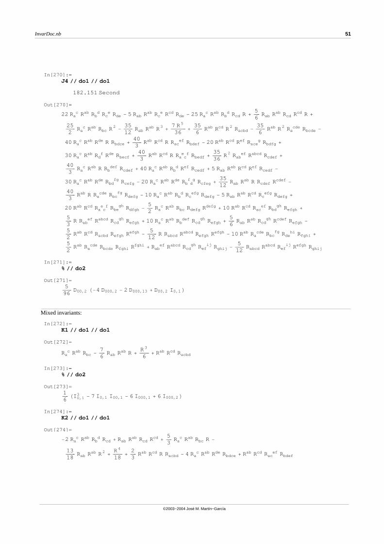
In[270]:=J4 �� do1 �� do1
182.151 Second
Out[270]=
22 Rac Rab Rb
d Rce Rde - 5 Rab Rab Rc
e Rcd Rde - 25 Rac Rab Rb
d Rcd R +5�����6
Rab Rab Rcd Rcd R +
25��������2
Rac Rab Rbc R2
-35��������12
Rab Rab R3+
7 R5
�������������36
+35��������6
Rab Rcd R2 Racbd -35��������6
Rab R2 Racde Rbcde -
40 Rac Rab Rde R Rbdce +
40��������3
Rab Rcd R Racef Rbdef - 20 Rab Rcd Ref Race
g Rbdfg +
30 Rac Rab Rd
f Rde Rbecf +40��������3
Rab Rcd R Ra ce f Rbedf +
35��������36
R2 Rabef Rabcd Rcdef +
40��������3
Rac Rab R Rb
def Rcdef + 40 Rac Rab Rb
d Ref Rcedf + 5 Rab Rab Rcd Ref Rcedf -
30 Rac Rab Rde Rbd
fg Rcefg - 20 Rac Rab Rde Rb d
f g Rcfeg +35��������12
Rab Rab R Rcdef Rcdef-
40��������3
Rab R Racde Rbc
fg Rdefg - 10 Rac Rab Rb
d Rcefg Rdefg - 5 Rab Rab Rcd Rc
efg Rdefg +
20 Rab Rcd Ra ce f Rbe
gh Rdfgh -5�����2
Rac Rab Rbc Rdefg Rdefg
+ 10 Rab Rcd Racef Rbd
gh Refgh +
5�����3
R Rabef Rabcd Rcd
gh Refgh + 10 Rac Rab Rb
def Rcdgh Refgh +
5�����6
Rab Rab Rcdgh Rcdef Refgh -
5�����2
Rab Rcd Racbd Refgh Refgh-
5��������12
R Rabcd Rabcd Refgh Refgh- 10 Rab Ra
cde Rbcfg Rde
hi Rfghi +
5�����2
Rab Racde Rbcde Rfghi Rfghi
+ Rabef Rabcd Rcd
gh Refij Rghij -
5��������12
Rabcd Rabcd Refij Refgh Rghij
In[271]:=% �� do2
Out[271]=5
��������96
D00,2 H-4 D000,2 - 2 D000,13 + D00,2 I 0,1 L
Mixed invariants:
In[272]:=K1 �� do1 �� do1
Out[272]=
Rac Rab Rbc -
7�����6
Rab Rab R +R3
��������6
+ Rab Rcd Racbd
In[273]:=% �� do2
Out[273]=1�����6HI 0,1
3- 7 I 0,1 I 00,1 - 6 I 000,1 + 6 I 000,2 L
In[274]:=K2 �� do1 �� do1
Out[274]=
-2 Rac Rab Rb
d Rcd + Rab Rab Rcd Rcd+
5�����3
Rac Rab Rbc R -
13��������18
Rab Rab R2+
R4
��������18
+2�����3
Rab Rcd R Racbd - 4 Rac Rab Rde Rbdce + Rab Rcd Rac
ef Rbdef
InvarDoc.nb 51
©2003−2004 José M. Martín−García
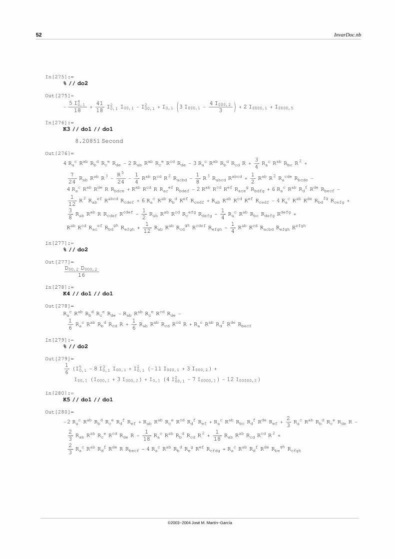
In[275]:=% �� do2
Out[275]=
-5 I 0,1
4
����������������18
+41��������18
I 0,12 I 00,1 - I 00,1
2+ I 0,1 J3 I 000,1 -
4 I 000,2��������������������
3N + 2 I 0000,1 + I 0000,5
In[276]:=K3 �� do1 �� do1
8.20851 Second
Out[276]=
4 Rac Rab Rb
d Rce Rde - 2 Rab Rab Rc
e Rcd Rde - 3 Rac Rab Rb
d Rcd R +3�����4
Rac Rab Rbc R2
+
7��������24
Rab Rab R3-
R5
��������24
-1�����4
Rab Rcd R2 Racbd -1�����8
R3 Rabcd Rabcd+
1�����2
Rab R2 Racde Rbcde -
4 Rac Rab Rde R Rbdce + Rab Rcd R Rac
ef Rbdef - 2 Rab Rcd Ref Raceg Rbdfg + 6 Ra
c Rab Rdf Rde Rbecf -
1��������12
R2 Rabef Rabcd Rcdef + 6 Ra
c Rab Rbd Ref Rcedf + Rab Rab Rcd Ref Rcedf - 4 Ra
c Rab Rde Rbdfg Rcefg +
3�����8
Rab Rab R Rcdef Rcdef-
1�����2
Rab Rab Rcd Rcefg Rdefg -
1�����4
Rac Rab Rbc Rdefg Rdefg
+
Rab Rcd Racef Rbd
gh Refgh +1
��������12
Rab Rab Rcdgh Rcdef Refgh -
1�����4
Rab Rcd Racbd Refgh Refgh
In[277]:=% �� do2
Out[277]=D00,2 D000,2�����������������������������
16
In[278]:=K4 �� do1 �� do1
Out[278]=
Rac Rab Rb
d Rce Rde - Rab Rab Rc
e Rcd Rde -
1�����6
Rac Rab Rb
d Rcd R +1�����6
Rab Rab Rcd Rcd R + Rac Rab Rd
f Rde Rbecf
In[279]:=% �� do2
Out[279]=1�����6HI 0,1
5- 8 I 0,1
3 I 00,1 + I 0,12 H-11 I 000,1 + 3 I 000,2 L +
I 00,1 HI 000,1 + 3 I 000,2 L + I 0,1 H4 I 00,12
- 7 I 0000,1 L - 12 I 00000,2 L
In[280]:=K5 �� do1 �� do1
Out[280]=
-2 Rac Rab Rb
d Rce Rd
f Ref + Rab Rab Rce Rcd Rd
f Ref + Rac Rab Rbc Rd
f Rde Ref +2�����3
Rac Rab Rb
d Rce Rde R -
2�����3
Rab Rab Rce Rcd Rde R -
1��������18
Rac Rab Rb
d Rcd R2+
1��������18
Rab Rab Rcd Rcd R2+
2�����3
Rac Rab Rd
f Rde R Rbecf - 4 Rac Rab Rb
d Reg Ref Rcfdg + Ra
c Rab Rdf Rde Rbe
gh Rcfgh
52 InvarDoc.nb
©2003−2004 José M. Martín−García
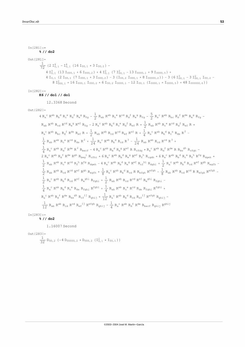
In[281]:=% �� do2
Out[281]=1
��������72H2 I 0,1
6- I 0,1
4 H16 I 00,1 + 3 I 00,2 L -
4 I 0,13 H13 I 000,1 + 6 I 000,2 L + 4 I 0,1
2 H7 I 00,12
- 13 I 0000,1 + 9 I 0000,5 L +
4 I 0,1 H2 I 00,1 H7 I 000,1 + 3 I 000,2 L - 3 HI 00,2 I 000,1 + 8 I 00000,2 LL - 3 H6 I 00,13
- 3 I 00,12 I 00,2 -
8 I 000,12
+ 16 I 000,1 I 000,2 + 6 I 00,2 I 0000,1 - 12 I 00,1 HI 0000,1 + I 0000,5 L + 48 I 000000,6 LL
In[282]:=K6 �� do1 �� do1
12.3368 Second
Out[282]=
4 Rac Rab Rb
d Rce Rd
f Reg Rfg -
1�����2
Rab Rab Rce Rcd Rd
f Reg Rfg -
5�����2
Rac Rab Rbc Rd
f Rde Reg Rfg -
Rab Rab Rcd Rcd Reg Ref Rfg - 2 Ra
c Rab Rbd Rc
e Rdf Ref R +
1�����2
Rab Rab Rce Rcd Rd
f Ref R +
Rac Rab Rbc Rd
f Rde Ref R +1�����2
Rab Rab Rcd Rcd Ref Ref R +1�����4
Rac Rab Rb
d Rce Rde R2
-
1�����4
Rab Rab Rce Rcd Rde R2
+1
��������24
Rac Rab Rb
d Rcd R3-
1��������24
Rab Rab Rcd Rcd R3+
1�����4
Rac Rab Rd
f Rde R2 Rbecf - 4 Rac Rab Rb
d Reg Ref R Rcfdg + Ra
c Rab Rdf Rde R Rbe
gh Rcfgh -
2 Rac Rab Rd
f Rde Rgh Rbegi Rcfhi + 6 Ra
c Rab Rbd Re
g Ref Rfh Rcgdh + 6 Ra
c Rab Rbd Rc
e Rfh Rfg Rdgeh +
1�����2
Rab Rab Rce Rcd Rf
h Rfg Rdgeh - 4 Rac Rab Rb
d Reg Ref Rcf
hi Rdghi +1�����2
Rac Rab Rb
d Rcd Ref Rgh Regfh -
1�����2
Rab Rab Rcd Rcd Ref Rgh Regfh +1�����8
Rac Rab Rb
d Rcd R Refgh Refgh-
1�����8
Rab Rab Rcd Rcd R Refgh Refgh-
1�����2
Rac Rab Rb
d Rcd Ref Reghi Rfghi +
1�����2
Rab Rab Rcd Rcd Ref Reghi Rfghi -
1�����4
Rac Rab Rb
d Rce Rde Rfghi Rfghi
+1�����4
Rab Rab Rce Rcd Rde Rfghi Rfghi
+
Rac Rab Rd
f Rde Rbegh Rcf
ij Rghij +1
��������12
Rac Rab Rb
d Rcd Refij Refgh Rghij -
1��������12
Rab Rab Rcd Rcd Refij Refgh Rghij -
1�����4
Rac Rab Rd
f Rde Rbecf Rghij Rghij
In[283]:=% �� do2
1.16007 Second
Out[283]=1
��������32
D00,2 H-4 D00000,2 + D000,2 HI 0,12
+ I 00,1 LL
InvarDoc.nb 53
©2003−2004 José M. Martín−García
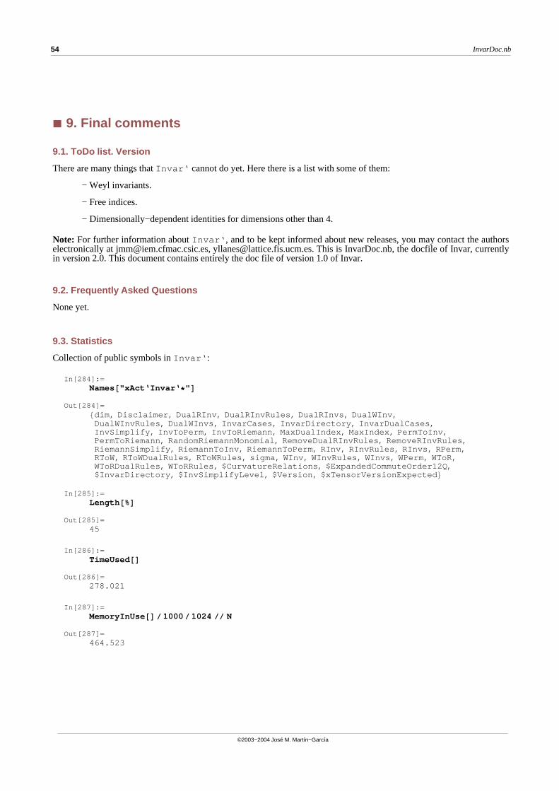
à 9. Final comments
9.1. ToDo list. Version
There are many things that Invar‘ cannot do yet. Here there is a list with some of them:
− Weyl invariants.
− Free indices.
− Dimensionally−dependent identities for dimensions other than 4.
Note: For further information about Invar‘ , and to be kept informed about new releases, you may contact the authorselectronically at [email protected], [email protected]. This is InvarDoc.nb, the docfile of Invar, currentlyin version 2.0. This document contains entirely the doc file of version 1.0 of Invar.
9.2. Frequently Asked Questions
None yet.
9.3. Statistics
Collection of public symbols in Invar‘ :
In[284]:=Names@"xAct‘Invar‘*"D
Out[284]=8dim, Disclaimer, DualRInv, DualRInvRules, DualRInvs, DualWInv,
DualWInvRules, DualWInvs, InvarCases, InvarDirectory, InvarDualCases,InvSimplify, InvToPerm, InvToRiemann, MaxDualIndex, MaxIndex, PermToInv,PermToRiemann, RandomRiemannMonomial, RemoveDualRInvRules, RemoveRInvRules,RiemannSimplify, RiemannToInv, RiemannToPerm, RInv, RInvRules, RInvs, RPerm,RToW, RToWDualRules, RToWRules, sigma, WInv, WInvRules, WInvs, WPerm, WToR,WToRDualRules, WToRRules, $CurvatureRelations, $ExpandedCommuteOrder12Q,$InvarDirectory, $InvSimplifyLevel, $Version, $xTensorVersionExpected <
In[285]:=Length@%D
Out[285]=45
In[286]:=TimeUsed@D
Out[286]=278.021
In[287]:=MemoryInUse@D�1000�1024 �� N
Out[287]=464.523
54 InvarDoc.nb
©2003−2004 José M. Martín−García
In[288]:=MaxMemoryUsed@D�1000�1024 �� N
Out[288]=484.799
InvarDoc.nb 55
©2003−2004 José M. Martín−García