Supporting Information for

X-ray absorption spectroscopy quantitative analysis of biomimetic copper(II) complexes with tridentate nitrogen ligands mimicking the tris(imidazole) array of protein centres Elena Borghi*a and Luigi Casellab

aDipartimento di Chimica, Università di Roma “La Sapienza”, Piazzale A. Moro 5, 00185 Roma, Italy and bDipartimento di Chimica Generale, Università di Pavia, via Taramelli 12, 27100 Pavia, Italy e.borghi@caspur.it and bioinorg@unipv.it

SI-1. MS XANES simulations The software procedure, MXAN1-3, is able to fit the XANES part of the experimental spectra. The method performs the fit between the experimental spectrum and several theoretical calculations obtained by changing a defined set of structural parameters around the absorbing atom. The MXAN method, properly taking into account all the multiple scattering contributions, calculates exactly the total photon absorption cross-section. The absorption coefficient is directly given as a function of the energy, allowing an immediate fit of the experimental data. The optimisation in parameter space is achieved using the MINUIT program of the CERN library by performing the minimisation of the square residual function S2 defined as:

( )[ ]

∑

∑

=

=

−−= m

1ii

m

1i

21expi

thii

2

w

yywnS

iε

where n is the number of independent parameters, m is the number of data points, yi

th and yiexp are the theoretical and

experimental values of absorption, respectively, εi is the individual error in the experimental data set, and wi is a statistical weight. For wi = constant = 1, the square residual function, S2, becomes the statistical χ2 function. The estimate of the experimental error represented by εi, was considered constant in the fitting procedure, and in this case, it was assumed equal to ~1% of the experimental edge jump. This procedure uses the set of programs developed at the INFN Laboratori Nazionali di Frascati4 by the Frascati theory group: VGEN, which is a generator of muffin-tin (MT) potentials, the CONTINUUM code for the full multiple scattering cross-section calculation. The MS calculations are done in the frame of one-electron theory by using a molecular electron potential calculated with the MT approximation. The MT potential is calculated around each atomic species (the MT spheres). The MT radii are chosen according to the Norman criterion, with specified percentage of overlap allowed between the contiguous spheres, and the potential is recalculated at each step of the minimization procedure keeping the overlap factor fixed. The Coulomb part of the potential is calculated using the atomic charge densities of Clementi and Roetti tables.5 The exchange correlation part of the potential can be calculated using the complex Hedin–Lundqvist (H-L) optical form.6 To avoid the over damping at low energies of the complex part of the HL potential in the case of covalent molecular systems, MXAN uses a phenomenological approach that takes into account the inelastic processes by a convolution of the theoretical spectrum with a broadening function. This calculation uses only the real part of the HL potential, with a suitable Lorentzian function having an energy-dependent width of the form Γtot(E ) = Γc + Γ(E). The constant part, Γc, is the energy independent broadening value, includes the core-hole lifetime and the experimental resolution. The energy-dependent term, Γ(E), represents all the inelastic processes, accounting for any damping associated with the inelastic losses of the photoelectron in the final state. Both parameters are refined during the fitting procedure. The Γ(E) function is zero below an onset energy, Es, (which corresponds to the plasmon excitation energy) and begins to increase from a value, As, (which corresponds to the plasmon excitation amplitude). Their numerical values are derived at each computational step of optimization of the structural parameters (i.e., for each geometric configuration) on the basis of a Monte Carlo fit. The MXAN method introduces four non-structural parameters (i.e. Fermi energy, broadening parameters (energy-independent/dependent), overlap between the MT radii). The coordination numbers and the Debye-Waller factors are not treated, the edge jump (normalization) and the edge position (alignment) are unrelated to the fitted structural parameters, so the relevant parameters are essentially geometrical. The non-structural parameters are refined by Monte Carlo search at each step. In a final minimization cycle to get parameters errors, and to avoid artificial results, they were fixed. The minimization strategy employed in this study uses as structural parameters the polar coordinates (distances and polar angles) of the first ligands to the absorbing atom, put in the center of the coordinate system. Atoms linked to the first ligands

1

in the input coordinate file rigidly follow the movements of these ligands without changing the relative position. The only statistical errors that can be calculated numerically by the MIGRAD routine are those on polar parameters of the first-shell donors. In the case of test system, the [Cu(2-BB)(N3)]+ cation, the right geometrical configuration has been recovered within an error of the order of 0.03-0.06 Å in the interatomic distances and about 3 degrees in the angle determination. For the [Cu(2-BB)(H2O)n]+ cation in the powdered complex [Cu(2-BB)(H2O)n](ClO4)·(H2O)2-n (n=1 or 2) the “true actual” configuration obtained for the two independent best-fitting simulations show an error of the order of 0.02-0.04 Å in bond distances and of 2-3 degrees in the angles. Ligand angles can be added in the input coordinate file, so that the program MXAN will provide automatically their best-fitting values. Furthermore the MXAN procedure supplies as output file the best fitting structure in a format readable by molecule viewer programs. All bond distances and bond angles, different from the first-shell ones, reported in Tables SI-1 1, SI-1 2, SI-1 3 have been evaluated with the Mercury program available from the Cambridge Crystallographic Data Centre.

2

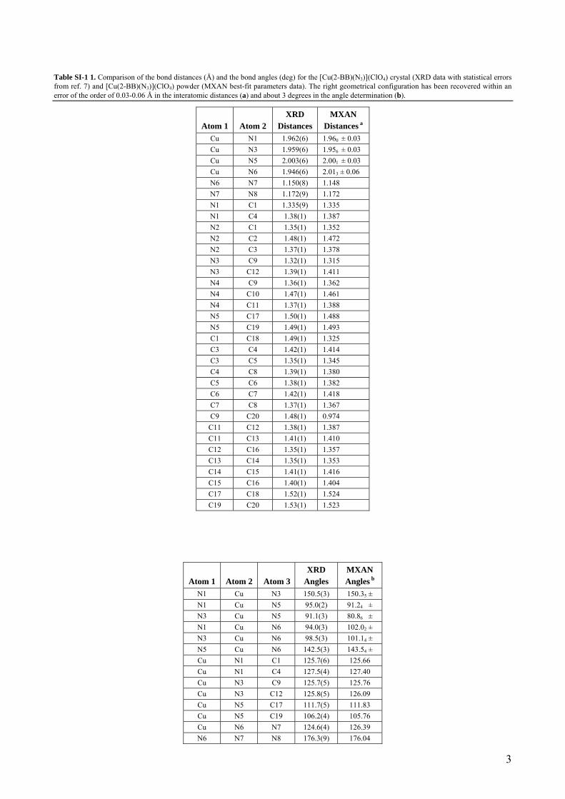
Table SI-1 1. Comparison of the bond distances (Å) and the bond angles (deg) for the [Cu(2-BB)(N3)](ClO4) crystal (XRD data with statistical errors from ref. 7) and [Cu(2-BB)(N3)](ClO4) powder (MXAN best-fit parameters data). The right geometrical configuration has been recovered within an error of the order of 0.03-0.06 Å in the interatomic distances (a) and about 3 degrees in the angle determination (b).

Atom 1

Atom 2

XRD Distances

MXAN Distances a

Cu N1 1.962(6) 1.960 ± 0.03 Cu N3 1.959(6) 1.956 ± 0.03 Cu N5 2.003(6) 2.001 ± 0.03 Cu N6 1.946(6) 2.013 ± 0.06 N6 N7 1.150(8) 1.148 N7 N8 1.172(9) 1.172 N1 C1 1.335(9) 1.335 N1 C4 1.38(1) 1.387 N2 C1 1.35(1) 1.352 N2 C2 1.48(1) 1.472 N2 C3 1.37(1) 1.378 N3 C9 1.32(1) 1.315 N3 C12 1.39(1) 1.411 N4 C9 1.36(1) 1.362 N4 C10 1.47(1) 1.461 N4 C11 1.37(1) 1.388 N5 C17 1.50(1) 1.488 N5 C19 1.49(1) 1.493 C1 C18 1.49(1) 1.325 C3 C4 1.42(1) 1.414 C3 C5 1.35(1) 1.345 C4 C8 1.39(1) 1.380 C5 C6 1.38(1) 1.382 C6 C7 1.42(1) 1.418 C7 C8 1.37(1) 1.367 C9 C20 1.48(1) 0.974 C11 C12 1.38(1) 1.387 C11 C13 1.41(1) 1.410 C12 C16 1.35(1) 1.357 C13 C14 1.35(1) 1.353 C14 C15 1.41(1) 1.416 C15 C16 1.40(1) 1.404 C17 C18 1.52(1) 1.524 C19 C20 1.53(1) 1.523

Atom 1

Atom 2

Atom 3

XRD Angles

MXAN Angles b

N1 Cu N3 150.5(3) 150.35 ± N1 Cu N5 95.0(2) 91.24 ± N3 Cu N5 91.1(3) 80.86 ± N1 Cu N6 94.0(3) 102.02 ± N3 Cu N6 98.5(3) 101.14 ± N5 Cu N6 142.5(3) 143.54 ± Cu N1 C1 125.7(6) 125.66 Cu N1 C4 127.5(4) 127.40 Cu N3 C9 125.7(5) 125.76 Cu N3 C12 125.8(5) 126.09 Cu N5 C17 111.7(5) 111.83 Cu N5 C19 106.2(4) 105.76 Cu N6 N7 124.6(4) 126.39 N6 N7 N8 176.3(9) 176.04

3

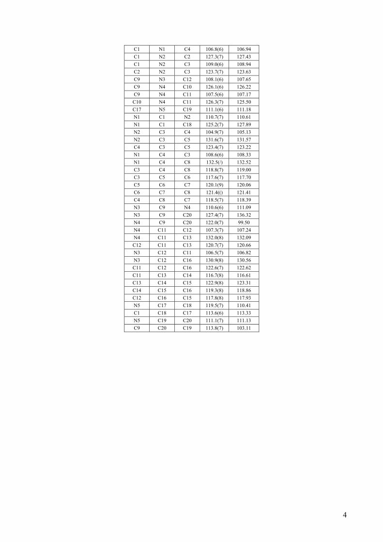
C1 N1 C4 106.8(6) 106.94 C1 N2 C2 127.3(7) 127.43 C1 N2 C3 109.0(6) 108.94 C2 N2 C3 123.7(7) 123.63 C9 N3 C12 108.1(6) 107.65 C9 N4 C10 126.1(6) 126.22 C9 N4 C11 107.5(6) 107.17 C10 N4 C11 126.3(7) 125.50 C17 N5 C19 111.1(6) 111.18 N1 C1 N2 110.7(7) 110.61 N1 C1 C18 125.2(7) 127.89 N2 C3 C4 104.9(7) 105.13 N2 C3 C5 131.6(7) 131.57 C4 C3 C5 123.4(7) 123.22 N1 C4 C3 108.6(6) 108.33 N1 C4 C8 132.5(/) 132.52 C3 C4 C8 118.8(7) 119.00 C3 C5 C6 117.6(7) 117.70 C5 C6 C7 120.1(9) 120.06 C6 C7 C8 121.4(() 121.41 C4 C8 C7 118.5(7) 118.39 N3 C9 N4 110.6(6) 111.09 N3 C9 C20 127.4(7) 136.32 N4 C9 C20 122.0(7) 99.50 N4 C11 C12 107.3(7) 107.24 N4 C11 C13 132.0(8) 132.09 C12 C11 C13 120.7(7) 120.66 N3 C12 C11 106.5(7) 106.82 N3 C12 C16 130.9(8) 130.56 C11 C12 C16 122.6(7) 122.62 C11 C13 C14 116.7(8) 116.61 C13 C14 C15 122.9(8) 123.31 C14 C15 C16 119.3(8) 118.86 C12 C16 C15 117.8(8) 117.93 N5 C17 C18 119.5(7) 110.41 C1 C18 C17 113.6(6) 113.33 N5 C19 C20 111.1(7) 111.13 C9 C20 C19 113.8(7) 103.11

4

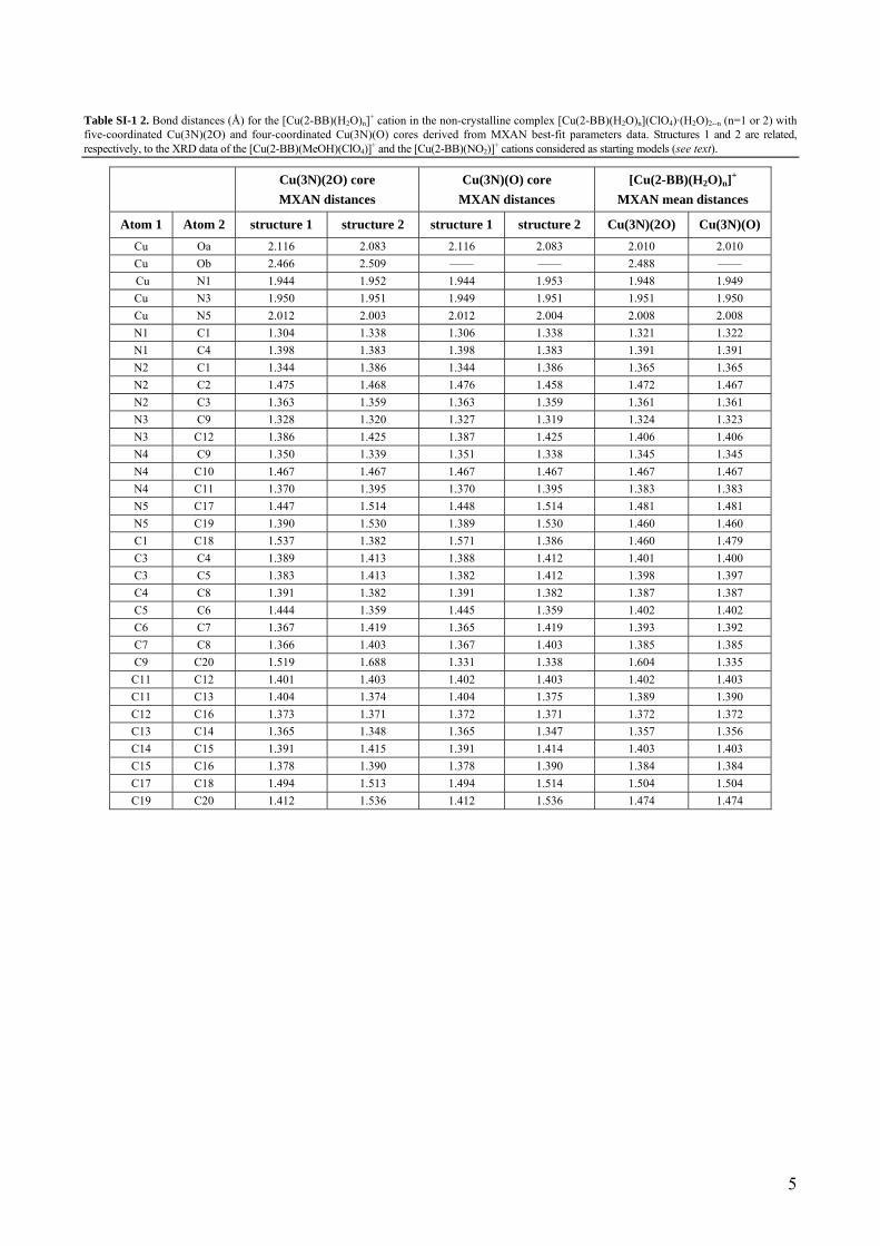
Table SI-1 2. Bond distances (Å) for the [Cu(2-BB)(H2O)n]+ cation in the non-crystalline complex [Cu(2-BB)(H2O)n](ClO4)·(H2O)2--n (n=1 or 2) with five-coordinated Cu(3N)(2O) and four-coordinated Cu(3N)(O) cores derived from MXAN best-fit parameters data. Structures 1 and 2 are related, respectively, to the XRD data of the [Cu(2-BB)(MeOH)(ClO4)]+ and the [Cu(2-BB)(NO2)]+ cations considered as starting models (see text).

Cu(3N)(2O) core MXAN distances

Cu(3N)(O) core MXAN distances

[Cu(2-BB)(H2O)n]+

MXAN mean distances

Atom 1 Atom 2 structure 1 structure 2 structure 1 structure 2 Cu(3N)(2O) Cu(3N)(O) Cu Oa 2.116 2.083 2.116 2.083 2.010 2.010 Cu Ob 2.466 2.509 —— —— 2.488 —— Cu N1 1.944 1.952 1.944 1.953 1.948 1.949 Cu N3 1.950 1.951 1.949 1.951 1.951 1.950 Cu N5 2.012 2.003 2.012 2.004 2.008 2.008 N1 C1 1.304 1.338 1.306 1.338 1.321 1.322 N1 C4 1.398 1.383 1.398 1.383 1.391 1.391 N2 C1 1.344 1.386 1.344 1.386 1.365 1.365 N2 C2 1.475 1.468 1.476 1.458 1.472 1.467 N2 C3 1.363 1.359 1.363 1.359 1.361 1.361 N3 C9 1.328 1.320 1.327 1.319 1.324 1.323 N3 C12 1.386 1.425 1.387 1.425 1.406 1.406 N4 C9 1.350 1.339 1.351 1.338 1.345 1.345 N4 C10 1.467 1.467 1.467 1.467 1.467 1.467 N4 C11 1.370 1.395 1.370 1.395 1.383 1.383 N5 C17 1.447 1.514 1.448 1.514 1.481 1.481 N5 C19 1.390 1.530 1.389 1.530 1.460 1.460 C1 C18 1.537 1.382 1.571 1.386 1.460 1.479 C3 C4 1.389 1.413 1.388 1.412 1.401 1.400 C3 C5 1.383 1.413 1.382 1.412 1.398 1.397 C4 C8 1.391 1.382 1.391 1.382 1.387 1.387 C5 C6 1.444 1.359 1.445 1.359 1.402 1.402 C6 C7 1.367 1.419 1.365 1.419 1.393 1.392 C7 C8 1.366 1.403 1.367 1.403 1.385 1.385 C9 C20 1.519 1.688 1.331 1.338 1.604 1.335 C11 C12 1.401 1.403 1.402 1.403 1.402 1.403 C11 C13 1.404 1.374 1.404 1.375 1.389 1.390 C12 C16 1.373 1.371 1.372 1.371 1.372 1.372 C13 C14 1.365 1.348 1.365 1.347 1.357 1.356 C14 C15 1.391 1.415 1.391 1.414 1.403 1.403 C15 C16 1.378 1.390 1.378 1.390 1.384 1.384 C17 C18 1.494 1.513 1.494 1.514 1.504 1.504 C19 C20 1.412 1.536 1.412 1.536 1.474 1.474

5

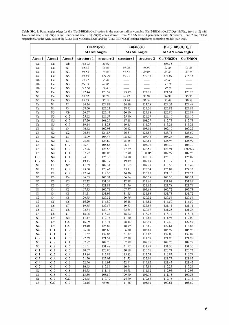
Table SI-1 3. Bond angles (deg) for the [Cu(2-BB)(H2O)n]+ cation in the non-crystalline complex [Cu(2-BB)(H2O)n](ClO4)·(H2O)2--n (n=1 or 2) with five-coordinated Cu(3N)(2O) and four-coordinated Cu(3N)(O) cores derived from MXAN best-fit parameters data. Structures 1 and 2 are related, respectively, to the XRD data of the [Cu(2-BB)(MeOH)(ClO4)]+ and the [Cu(2-BB)(NO2)]+ cations considered as starting models (see text).

Cu(3N)(2O) MXAN Angles

Cu(3N)(O) MXAN Angles

[Cu(2-BB)(H2O)2]+

MXAN mean angles

Atom 1 Atom 2 Atom 3 structure 1 structure 2 structure 1 structure 2 Cu(3N)(2O) Cu(3N)(O) Oa Cu Ob 146.08 65.02 —— —— 105.55 —— Oa Cu N1 85.32 98.03 91.20 98.90 91.68 95.05 Oa Cu N3 96.63 75.03 87.83 80.06 85.83 83.95 Oa Cu N5 86.95 141.23 99.75 137.35 114.09 118.55 Ob Cu N1 75.41 95.84 —— —— 85.63 —— Ob Cu N3 99.33 87.05 —— —— 93.19 —— Ob Cu N5 122.68 76.83 —— —— 99.76 —— N1 Cu N3 172.44 170.57 173.79 172.70 171.51 173.25 N1 Cu N5 97.62 92.22 96.77 93.97 94.92 95.37 N3 Cu N5 89.79 97.18 89.44 91.59 93.49 90.52 Cu N1 C1 124.24 124.81 124.19 124.78 124.53 124.49 Cu N1 C4 128.50 127.23 128.53 127.20 127.82 127.87 Cu N3 C9 126.57 127.14 126.60 127.18 126.86 126.89 Cu N3 C12 125.62 126.57 125.60 126.59 126.10 126.10 Cu N5 C17 117.20 108.29 117.18 108.27 112.75 112.73 Cu N5 C19 119.14 111.28 119.15 111.27 115.21 115.21 C1 N1 C4 106.42 107.95 106.42 108.02 107.19 107.22 C1 N2 C2 126.54 124.88 126.51 124.87 125.71 125.69 C1 N2 C3 108.09 108.46 108.12 108.45 108.28 108.29 C2 N2 C3 125.35 126.60 125.35 126.62 125.98 125.99 C9 N3 C12 106.81 105.83 106.81 105.78 106.32 106.30 C9 N4 C10 127.26 126.56 127.29 126.56 126.91 126.925 C9 N4 C11 107.92 108.06 107.90 108..05 107.99 107.98 C10 N4 C11 124.81 125.38 124.80 125.38 125.10 125.09 C17 N5 C19 119.15 107.19 119.19 107.19 113.17 113.19 N1 C1 N2 111.69 109.31 111.62 109.28 110.50 110.45 N1 C1 C18 123.60 128.43 123.11 125.54 126.02 124.33 N2 C1 C18 122.84 119.36 124.30 120.15 121.10 122.23 N2 C3 C4 106.03 106.57 106.04 106.58 106.30 106.31 N2 C3 C5 132.22 131.59 132.18 131.60 131.91 131.89 C4 C3 C5 121.72 121.84 121.76 121.82 121.78 121.79 N1 C4 C3 107.73 107.71 107.77 107.68 107.72 107.73 N1 C4 C8 131.51 131.94 131.45 131.98 131.73 131.72 C3 C4 C8 120.75 120.32 120.76 120.32 120.54 120.54 C3 C5 C6 116.20 116.80 116.18 116.82 116.50 116.50 C5 C6 C7 119.65 122.57 119.63 122.58 121.11 121.11 C6 C7 C8 122.34 120.16 122.35 120.17 121.25 121.26 C4 C8 C7 118.06 118.27 118.02 118.25 118.17 118.14 N3 C9 N4 111.17 112.73 111.20 112.80 111.95 112.00 N3 C9 C20 116.09 118.71 128.14 126.99 117.40 127.57 N4 C9 C20 119.40 125.82 118.99 118.66 122.61 118.83 N4 C11 C12 106.28 105.66 106.30 105.61 105.97 105.96 N4 C11 C13 131.32 132.83 131.32 132.82 132.08 132.07 C12 C11 C13 122.39 121.51 122.38 121.57 121.95 121.98 N3 C12 C11 107.82 107.70 107.79 107.75 107.76 107.77 N3 C12 C16 131.51 131.48 131.52 131.47 131.50 131.50 C11 C12 C16 120.67 120.80 120.69 120.76 120.74 120.73 C11 C13 C14 115.84 117.81 115.83 117.74 116.83 116.79 C13 C14 C15 121.50 122.03 121.53 122.10 121.77 121.82 C14 C15 C16 122.96 119.93 122.91 119.92 121.45 121.42 C12 C16 C15 116.63 117.86 116.64 117.84 117.25 117.24 N5 C17 C18 114.73 111.16 114.78 111.12 112.95 112.95 C1 C18 C17 113.36 108.89 109.90 104.75 111.13 107.33 N5 C19 C20 124.75 110.70 124.79 110.68 117.73 117.74 C9 C20 C19 102.16 99.06 111.86 105.92 100.61 108.89

6

Table SI-1 4. MXAN best-fit results for the non-structural parameters

broadening parameters error (S2)

structure overlap factor (%)

Fermi energy

Γc (eV) Γ(E) Es (eV) As

Cu(2-BB)(N3) 3.4 -1.88 2.22 25.16 9.69 0.30

Cu(2-BB)(2O) (a) 5.4 -1.05 2.35 16.52 11.91 0.22

Cu(2-BB)(O) (a) 6.3 -0.27 2.43 17.30 12.13 0.21

Cu(2-BB)(2O) (b) 4.3 - 0.95 2.30 16.99 14.23 0.21

Cu(2-BB)(O) (b) 4.7 - 0.45 2.41 17.88 14.60 0.21

The values of the error function (S2) indicate that the agreement between the theoretical and experimental data is very good in the energy region chosen for the simulations. The values of Γc are reasonable considering that the core-hole lifetime width of copper is 1.55 eV.8

(a) and (b) refer to the best-fits from, respectively, the XRD data of the [Cu(2-BB)(MeOH)(ClO4)]+ and of the [Cu(2-BB)(NO2)]+ cations considered as starting models with five- and four-coordinated cores. See text.

Figure SI-1 1. Theoretical full MS cross-section calculations with the CONTINUUM code of the Cu K-edge absorption of the mononuclear complexes of the 2-BB ligand with different coordination geometries. Clusters of atoms corresponding to the entire cationic complexes have been considered. (a) [Cu(2-BB)N3]+ cation complex, (b) [Cu(2-BB)(MeOH)(ClO4)]+ cation complex, (c) [Cu(2-BB)(NO2)]+ cation complex. Reproduced from ref. 9.

References SI-1 1 M. Benfatto and S. Della Longa, J. Synchrotron Radiat. 2001, 8, 1087–1094. 2 M. Benfatto, S. Della Longa, and C. R.Natoli, J. Synchrotron Radiat. 2003, 10, 51-57 3 C. R. Natoli, M. Benfatto, S. Della Longa and K. Hatada, J. Synchrotron Radiat. 2003, 10, 26-42. 4 T. A. Tyson, K. O. Hodgson, C. R. Natoli and M. Benfatto, Phys. Rev. B 1992, 46, 5997-6019. 5 E. Clementi and C. Roetti, Atom. Data Nucl. Data Tables 1974, 14, 177-478. 6 L. Hedin and B. I. Lundqvist, J. Phys. C 1971, 4, 2064-2083. 7 L. Casella, O. Cargo, M. Gullotti, S. Doldi and M. Frassoni, Inorg. Chem. 1996, 35, 1101-1113. 8 M. O. Krause and H. H: Oliver, J. Phys. Chem. Ref. Data 1979, 8, 329-338. 9 E. Borghi and P. L. Solari, J. Synchrotron Radiat. 2005, 12, 102-110.

7

Supporting Information for

X-ray absorption spectroscopy quantitative analysis of biomimetic copper(II) complexes with tridentate nitrogen ligands mimicking the tris(imidazole) array of protein centres Elena Borghi*a and Luigi Casellab

aDipartimento di Chimica, Università di Roma “La Sapienza”, Piazzale A. Moro 5, 00185 Roma, Italy and bDipartimento di Chimica Generale, Università di Pavia, via Taramelli 12, 27100 Pavia, Italy e.borghi@caspur.it and bioinorg@unipv.it

SI-2. EXAFS analysis in multiple-scattering (MS) formalism: the MS theoretical calculations considered to achieve a good fit of the experimental spectrum of the [Cu(2-BB)(H2O)n](ClO4)·(H2O)2-n (n=1 or 2) complex in powder form The EXAFS analysis has been performed using the GNXAS set of programs. This code, which takes full account of the MS effects, is particularly suited for analyzing disordered systems and has been successfully applied to investigate biological or biological-related samples. The GNXAS program, given an atomic cluster [i.e. the model structure], finds all inequivalent absorbers, calculates ab-initio the associate signals and compares their sum to the experimental signal. The ability of the method in reproducing known structures in test cases has been amply documented in the literature. The theoretical signal is subsequently refined against the experimental signal in order to determine the structural parameters of the sample. With GNXAS, differently from other advanced analysis codes, starting from the model structure, the total theoretical EXAFS χ(k) signal is not decomposed as a sum of signals related to the number of scattering events [i.e. χ(2), χ(3), χ(4)] but as a sum of signals related to the different two-body, three-body and four-body sub-geometries inside the system of atoms [i.e. γ(2), γ(3) and γ(4)]. The structural parameters associated with a generic n-body signals [i.e. the multiplicity N, the distances R, the angles θ, the dihedral angles ψ and their associated Deby

1-3

e Waller (DW) factors, σ2] can be obtained with best fits [for more details see, for example, Di Cicco (2003)4]. Distinguishing the multiplicity of the n-body signals and taking into account the single and multiple scatterings coming from the n-atoms, the theoretical EXAFS signal is calculated as

χ(k) = ∑ γ(2) + γ(3) + γ(4)

In order to avoid signal proliferation in a fitting procedure it is essential to group the signals associated with the same n-atom configuration. This procedure is convenient to reduce the calculation parameters especially in the case of leading signals with comparable frequencies. A typical example is that of a structure with a first coordination shell and a second coordination shell. The second shell atom will be first shell of the first shell, therefore each second shell distance is also part of a triangle with an additional intermediate first shell atom. In this case the grouping procedure can combine the γ(n) signals with different n values involving sub-clusters of the main n-atom configuration, considering the n-body signal η(n) defined as

n-1

η(n) = γ(n) + ∑ γ(j) j=2

Thus, for a three-body configuration, the corresponding η(3) signal consists of a three-body γ(3) signal and a γ(2) signal between the two more distant atoms (γLB(2), LB=long-bond signal), [i.e. η(3) = γ(3) + γLB(2)]. An effective four-body η(4) signal consists of a two-body long-bond signal, of a three body signals, and of a four-body signal, [i.e. η(4) = γ(4) + γ(3)+ γLB(2)]. The refined MS results, 5, 6 including the previously unpublished values of the angular parameters, for the hypothetical [Cu(2-BB)(H2O)2](ClO4) complex in the [Cu(2-BB)(H2O)n](ClO4)·(H2O)2-n (n=1 or 2) powder form, obtained by taking as a starting structure the XRD data of the [Cu(2-BB)(MeOH)(ClO4)](ClO4) complex, 7 are presented in Table SI-2 1. Figure SI-2 1 shows the crystal structure and the related 28-atoms cluster used in the fit. Figure SI-2 2 shows the n-body scattering paths considered for the EXAFS fit. The results of the fit for the EXAFS signal, including details of the different theoretical signals used, are shown in Figure SI-2 3.

1

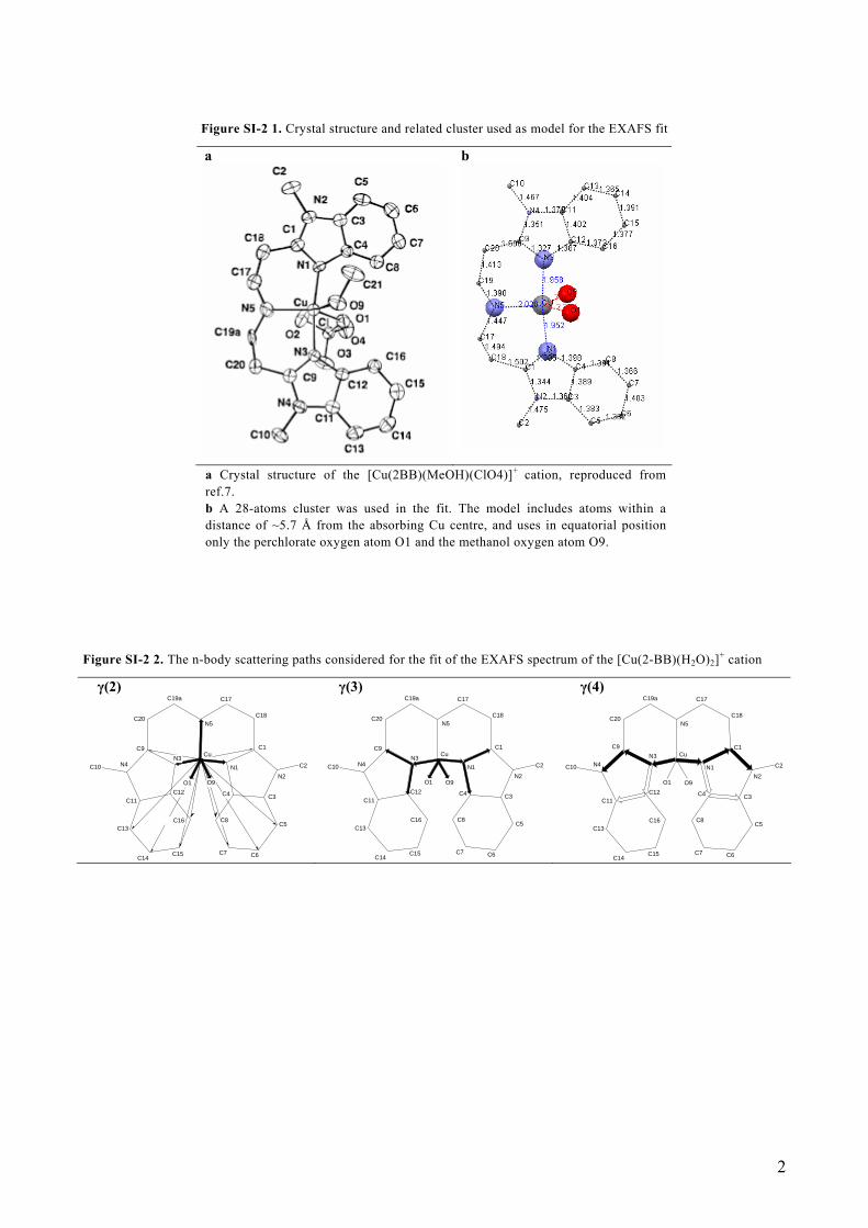
Figure SI-2 1. Crystal structure and related cluster used as model for the EXAFS fit

a b

a Crystal structure of the [Cu(2BB)(MeOH)(ClO4)]+ cation, reproduced from ref.7. b A 28-atoms cluster was used in the fit. The model includes atoms within a distance of ~5.7 Å from the absorbing Cu centre, and uses in equatorial position only the perchlorate oxygen atom O1 and the methanol oxygen atom O9.

Figure SI-2 2. The n-body scattering paths considered for the fit of the EXAFS spectrum of the [Cu(2-BB)(H2O)2]+ cation

γ(2)

C14C15

C13

C10

C11

C16 C8

C7 C6

C5

C3

N4Cu

C12

N3 C9

C20

C19a

N5

C17

C18

C1

C2N1

C4

N2O9O1

γ(3)

C14C15

C13

C10

C11

C16 C8

C7 C6

C5

C3

N4Cu

C12

N3 C9

C20

C19a

N5

C17

C18

C1

C2N1

C4

N2O9O1

γ(4)

C14C15

C13

C10

C11

C16 C8

C7 C6

C5

C3

N4Cu

C12

N3 C9

C20

C19a

N5

C17

C18

C1

C2N1

C4

N2O9O1

2

Figure SI-2 3. Detail of the theoretical signals considered for the final fit of the spectrum of the [Cu(2-BB)(H2O)2]+ cation

2 4 6 8 10 12

k (Å-1)

γ(2)Cu-N5

γ(2)Cu-N1/N3

γ(2)Cu-O9

γ(2)Cu-O1

γ(2)Cu-C1/C9

γ(2)Cu-C8/C16

γ(2)Cu-C7/C15

γ(2)Cu-C6/C14

γ(2)Cu-C5/C13

γ(3)Cu-N-C

γ(3)O-Cu-O

η(4)Cu-N1-C1-N2

η(4)Cu-N1-C4-C3

Residual experiment

Theory and experiment signals

χ(k

) x k

3 (a. u

.)

3

Table SI-2 1. Results obtained for the hypothetical [Cu(2-BB)(H2O)2]+ cation in the [Cu(2-BB)(H2O)n](ClO4)·(H2O)2-n powdered complex starting from the structure of [Cu(2BB)(MeOH)(ClO4)]+ cation

n-body scattering paths inside the cluster of 28 atoms

Distance (Å) or angle (°)

Structural parameter

Structural feature x multiplicity

XRD

Distance (Å)

σdist

2(Å2) or

n-body Signal associated

σang2 (°2) or angle (°)

Two-body scattering paths Cu(o)–N/O/C(i) γ(2) Ro,i Cu–N5 x 1 2.01 0.002 2.02 Cu–N1/N3 x 2 1.97 0.001 1.96 Cu–O9 x 1 2.30 0.006 2.11 Cu–O1 x 1 2.58 0.001 2.33 Cu–C1/C9 x 2 3.19 0.009 2.92 Cu–C8/C16 x 2 3.45 0.008 3.38 Cu–C7/C15 x 2 5.07 0.003 4.90 Cu–C6/C14 x 2 5.75 0.01 5.42 Cu–C5/C13 x 2 5.50 0.01 5.62 Three-body scattering paths inside imidazole: Cu(o)–N1(i)–C1/C4(j) and Cu(o)–N3(i)–C9/C12(j) Ro,i Cu–N1/N3 x 2 1.97 0.001 2.02 Ri,j N1–C1/C4 ; N3–C9/C12 x 4 1.30 0.001 1.30 θoij Cu–N1–C1/C4 ; Cu–N3–C9/C12 x 4 126.1 2.35 125.7 η(3)= γ(3)+γLB(2) Ro,j Cu–C1/C4 ; Cu–C9/C12 x 4 2.963 0.006 2.92 Three-body scattering path: O(i)–Cu(o)–O(j) γ(3) Ro,i Cu–O9 x 1 2.30 0.001 2.10 Ri,j Cu–O1 x 1 2.58 0.006 2.33 θoij O9–Cu–O1 x 1 127.0 1.07 119.1 Four-body scattering paths inside imidazole: Cu(o)–N1(i)–C1(j)–N2(k) and Cu(o)–N3(i)–C9(j)–N4(k) γ(4) Ro,i Cu–N1/N3 x 2 1.97 0.001 1.96 Ri,j N1/N3–C1/C9 x 2 1.30 0.001 1.31 θoij Cu–N1/N3–C1/C9 x 2 126.1 2.35 125.7 Rj,k C1/C9–N2/N4 x2 1.35 0.001 1.36 φijk N1/N3–C1/C9–N2/N4 x 2 109.9 16.43 110.4 Ψ (Ri,j) 170.6 15.1 170.6 η(4)=γ(4)+γLB(3) Ro,k Cu–N2/N4 x 2 4.10 0.006 4.12 Four-body scattering paths inside imidazole: Cu(o)–N1(i)–C4(j)–C3(k) and Cu(o)–N3(i)–C12(j)–C11(k) γ(4) Ro,i Cu–N1/N3 x 2 1.97 0.001 1.96 Ri,j N1/N3–C4/C12 x2 1.44 0.001 1.40 θoij Cu–N1/N3–C4/C12 x2 128.5 1.047 128.5 Rj,k C4/C12–C3/C11 x 2 1.38 0.003 1.39 φijk N1/N3–C4/C12–C3/C11 x2 109.9 16.43 107.8 ψ (Ri,j) 170.6 15.1 171.4 η(4)= γ(4)+ γLB(3) Ro,k Cu–C3/C11 x 2 4.22 0.016 4.19

Residual, experiment 0.806 x 10-6

4

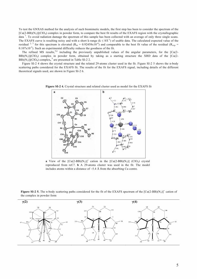
To test the GNXAS method for the analysis of such biomimetic models, the first step has been to consider the spectrum of the [Cu(2-BB)(N3)](ClO4) complex in powder form, to compare the best fit results of the EXAFS region with the crystallographic data 7. To avoid radiation damage the spectrum of this sample has been collected with an average of only three single scans. The EXAFS curve is resulting noisy and with a short k-range (k ≤ 8Å-1) of usable data. The calculated expected value of the residual 2, 3 for this spectrum is elevated (Rth = 0.92458x10-6) and comparable to the best fit value of the residual (Rexp = 0.107x10-5). Such an experimental difficulty reduces the goodness of the fit. The refined MS results,5,6 including the previously unpublished values of the angular parameters, for the [Cu(2-BB)(N3)](ClO4) complex in powder form, obtained by taking as a starting structure the XRD data of the [Cu(2-BB)(N3)](ClO4) complex, 7 are presented in Table SI-2 2. Figure SI-2 4 shows the crystal structure and the related 29-atoms cluster used in the fit. Figure SI-2 5 shows the n-body scattering paths considered for the EXAFS fit. The results of the fit for the EXAFS signal, including details of the different theoretical signals used, are shown in Figure SI-2 6.

Figure SI-2 4. Crystal structure and related cluster used as model for the EXAFS fit

a

b

a View of the [Cu(2-BB)(N3)]+ cation in the [Cu(2-BB)(N3)] (ClO4) crystal reproduced from ref.7. b A 29-atoms cluster was used in the fit. The model includes atoms within a distance of ~5.4 Å from the absorbing Cu centre.

Figure SI-2 5. The n-body scattering paths considered for the fit of the EXAFS spectrum of the [Cu(2-BB)(N3)]+ cation of the complex in powder form

γ(2)

γ(3) γ(4)

5

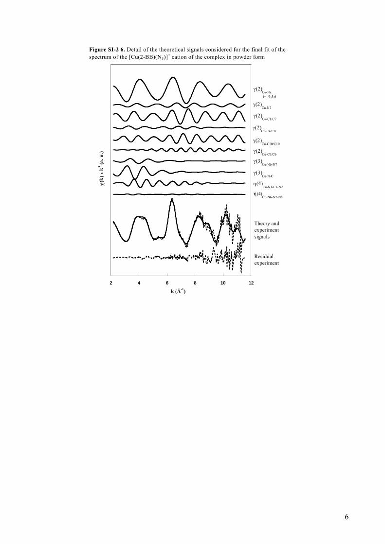
Figure SI-2 6. Detail of the theoretical signals considered for the final fit of the spectrum of the [Cu(2-BB)(N3)]+ cation of the complex in powder form

2 4 6 8 10 12

k (Å-1)

γ(2)Cu-Ni

γ(2)Cu-C1/C7

γ(2)Cu-C6/C6

η(4)Cu-N6-N7-N8

η(4)Cu-N1-C1-N2

γ(3)Cu-N-C

γ(3)Cu-N6-N7

γ(2)Cu-C4/C8

γ(2)Cu-C10/C10

γ(2)Cu-N7

χ(k

) x k

3 (a. u

.)

Theory and experiment signals

Residual experiment

i=1/3;5;6

6

Table SI-2 2. Results obtained for the [Cu(2-BB)(N3)]+ cation of the complex in powder form starting from the structure of the [Cu(2-BB)(N3)]+ cation in the [Cu(2-BB)(N3)](ClO4) crystal

n-body scattering paths inside the cluster of 29 atoms

Structural parameter

Structural feature x multiplicity

Distance (Å) or angle (°)

XRD

Distance (Å)

σdist

2(Å2) or

σang2 (°2)

n-body Signal associated

or angle (°)

Two-body scattering paths Cu(o)–N/C(i) γ(2) Ro,i Cu–N5 x 1 2.00 Cu–N1/N3 x 2 1.96 Cu–N6 x 1

0.002 1.96

1.95

Cu–N7 x 1 2.75 0.007 2.79 Cu–C1/C7 x 2 2.96 0.003 2.93 Cu–C4/C8 x 2 3.22 0.009 3.00 Cu–C5/C10 x 4 3.56 0.001 3.37 Cu–C6 x 2 4.94 0.001 4.90 Three-body scattering paths inside imidazole: Cu(o)–N1(i)–C1/C4(j) and Cu(o)–N3(i)–C7/C8(j) Ro,i Cu–N1/N3 x 2 1.96 0.002 1.96 Ri,j N1–C1/C4 ; N3–C7/C8 x 4 1.35 0.003 1.32 θoij Cu–N1–C1/C4 ; Cu–N3–C7/C8 x 4 126.6 24.18 125.7 η(3)= γ(3)+γLB(2) Ro,j Cu–C1/C4 ; Cu–C7/C8 x 4 2.78 0.008 2.86

Three-body scattering path: Cu(o)–N6(i)–N7(j) Ro,i Cu–N6 x 1 1.96 0.002 1.95 Ri,j N6–N7 x 1 1.11 0.001 1.15 θoij Cu–N6–N7 x 1 125.0 15.21 126.3

η(3)= γ(3)+γLB(2) Ro,j Cu–N7 x 1 2.78 0.006 2.79

Four-body scattering paths inside imidazole: Cu(o)–N1(i)–C1(j)–N2(k) and Cu(o)–N3(i)–C7(j)–N4(k) γ(4) Ro,i Cu–N1/N3 x 2 1.96 0.002 1.96 Ri,j N1/N3–C1/C7 x 2 1.34 0.004 1.34 θoij Cu–N1/N3–C1/C7 x 2 127.8 15.21 125.7 Rj,k C1/C7–N2/N4 x2 1.30 0.001 1.35 φijk N1/N3–C1/C7–N2/N4 x 2 112.7 23.33 110.6

ψ (Ri,j) 182.4 1.3 178.1 η(4)=γ(4)+γLB(3) Ro,k Cu–N2/N4 x 2 4.10 0.006 4.12

Four-body scattering paths inside azide: Cu(o)–N6(i)–N7(j)–N8(k) γ(4) Ro,i Cu–N6 x 1 1.96 0.002 1.95 Ri,j N6–N7 x 1 1.11 0.003 1.15 θoij Cu–N6–N7 x 1 127.5 15.21 126.3 Rj,k N7–N8 x 1 1.11 0.003 1.17 φijk N6–N7–N8 x 1 176.3 1.0 176.3 ψ (Ri,j) 163.3 15.16 164.4 η(4)= γ(4)+ γLB(3) Ro,k Cu–N8 x 1 4.22 0.016 4.19

Residual, experiment 0.107x 10-5

References SI-2 1 A. Filipponi, A. Di Cicco and C. R. Natoli, Phys. Rev. B 1995, 52, 15122-15134. 2 A. Filipponi and A.Di Cicco, Phys. Rev. B 1995, 52, 15135-15149. 3 A. Filipponi and A. Di Cicco, Task Q. 2000, 4, 575- 669. 4 A. Di Cicco, J. Synchrotron Rad. 2003, 10, 46-50. 5 E. Borghi, P. L: Solari, M. Beltramini, l. Bubacco, P. Di Muro and B. Salvato, Biophys. J. 2002, 82, 3254–3268. 6 M. Friello and E. Borghi, http://www.circmsb.uniba.it/ 2003 7 L. Casella, O. Cargo, M. Gullotti, S. Doldi and M. Frassoni, Inorg. Chem. 1996, 35, 1101-1113

7