X Marks the Spot: Nexus of Filaments, Cores,and Outflows in a Young Star-forming Region

Item Type Article

Authors Imara, Nia; Lada, Charles; Lewis, John; Bieging, John H.; Kong,Shuo; Lombardi, Marco; Alves, Joao

Citation X Marks the Spot: Nexus of Filaments, Cores, and Outflows in aYoung Star-forming Region 2017, 840 (2):119 The AstrophysicalJournal

DOI 10.3847/1538-4357/aa6d74

Publisher IOP PUBLISHING LTD

Journal The Astrophysical Journal

Rights © 2017. The American Astronomical Society. All rights reserved.

Download date 24/07/2018 05:11:03

Link to Item http://hdl.handle.net/10150/624336

X Marks the Spot: Nexus of Filaments, Cores, and Outflowsin a Young Star-forming Region

Nia Imara1, Charles Lada1, John Lewis1, John H. Bieging2, Shuo Kong3, Marco Lombardi4, and Joao Alves51 Harvard-Smithsonian Center for Astrophysics, 60 Garden Street, Cambridge, MA 02138, USA; nimara@cfa.harvard.edu

2 Steward Observatory, The University of Arizona, Tucson, AZ 85719, USA3 Department of Astronomy, Yale University, 52 Hillhouse Avenue, New Haven, CT 06511, USA

4 University of Milan, Department of Physics, via Celoria 16, I-20133, Italy5 University of Vienna, Türkenschanzstrasse 17, A-1880 Vienna, Austria

Received 2017 February 24; revised 2017 April 13; accepted 2017 April 14; published 2017 May 15

Abstract

We present a multiwavelength investigation of a region of a nearby giant molecular cloud that is distinguished by aminimal level of star formation activity. With our new CO12 (J=2–1) and CO13 (J=2–1) observations of a remoteregion within the middle of the California molecular cloud, we aim to investigate the relationship betweenfilaments, cores, and a molecular outflow in a relatively pristine environment. An extinction map of the region fromHerschel Space Observatory observations reveals the presence of two 2 pc long filaments radiating from a high-extinction clump. Using the CO13 observations, we show that the filaments have coherent velocity gradients andthat their mass-per-unit-lengths may exceed the critical value above which filaments are gravitationally unstable.The region exhibits structure with eight cores, at least one of which is a starless, prestellar core. We identify a low-velocity, low-mass molecular outflow that may be driven by a flat spectrum protostar. The outflow does not appearto be responsible for driving the turbulence in the core with which it is associated, nor does it provide significantsupport against gravitational collapse.

Key words: dust, extinction – ISM: clouds – ISM: jets and outflows – ISM: kinematics and dynamics – ISM:structure – stars: formation

1. Introduction

Observations show that the internal structures of giantmolecular clouds (GMCs) are permeated with complexsubstructure, including networks of filaments on a wide rangeof spatial scales, molecular outflows, and newly forming stars.In optical, submillimeter, and far-infrared images, filaments arefrequently seen radiating from compact groups of young stellarobjects (YSOs) and prestellar cores (e.g., Myers 2009; Andréet al. 2010; Ward-Thompson et al. 2010; André et al. 2014).Millimeter observations have revealed that YSOs, in turn, arefrequently associated with molecular outflows, which maydrive a significant portion of turbulence in GMCs (e.g., Ballyet al. 1996; Reipurth & Bally 2001; Maury et al. 2009). Theubiquity of such features suggests that outflows and filamentsplay critical roles in star formation (e.g., Margulis et al. 1988;Maury et al. 2009; Arzoumanian et al. 2011; Hacar et al. 2016).In particular, molecular line studies of nearby filamentarystructure demonstrate that prestellar core formation depends oncloud kinematics and chemistry (e.g., Duarte-Cabralet al. 2010; Hacar & Tafalla 2011; Arzoumanian et al. 2013;Kirk et al. 2013).

In this paper, we present results on the California molecularcloud (CMC), an excellent laboratory for studying the influenceof environment, structure, and cloud evolution on the initialconditions of star formation. At a distance of 450±23 pc(Lada et al. 2009; Lombardi et al. 2010), the CMC has a similarmass, size, and morphology to the Orion A molecular cloud(OMC). However,the CMC has a much lower level of starformation activity than the OMC does, with roughly an order ofmagnitude fewer YSOs (Lada et al. 2009, 2010). The mostobvious area of star formation within the CMC is the youngembedded cluster associated with the reflection nebula NGC1579 (Andrews & Wolk 2008), located at the southeastern edge

of the cloud. The cluster contains the B star Lk Hα 101, themost massive star known in the CMC. In dust extinction maps,one finds that the majority of the YSOs in the cloud areassociated with regions of highest extinction (Lada et al. 2009;Harvey et al. 2013). Most observed YSOs, in fact, are projectedalong a slender filamentary ridge in the south of the cloud(Lada et al. 2009; Harvey et al. 2013). As one proceedswestward in the CMC, one encounters regions of fewer YSOs,sometimes only single objects, and regions with no apparentstar formation activity at all. Thus, not only is the CMC notablefor its low level of star formation activity compared to moreactive GMCs in the solar vicinity, but within the cloud itselfthere appears to be a gradient in the star formation rate that isworthy of examination.The focus of this study is on a small region in the middle of

the CMC, near (l, b)=(162°.4, −8°.8), for which we presentnew CO12 (J=2–1) and CO13 (J=2–1) observations taken atthe Arizona Radio Observatory. These observations weremotivated in part by a noteworthy feature previously observedin an extinction map: two filaments radiating from a high-density structure with two embedded massive cores. As we willshow, the high-density structure from which the filamentsradiate also contains an outflow of molecular gas that is mostevident in CO12 emission. The filaments themselves are mostprominent in dust extinction. Altogether, the structure asobserved in extinction resembles an “X,” and we willhenceforth refer to it as California-X, or Cal-X. Near theoutflow, infrared observations reveal the presence of two brightsources, one of which is a YSO candidate that could be drivingthe outflow. While a number of studies have consideredfilaments feeding into clusters (e.g., Myers 2009; Schneideret al. 2012; André et al. 2016), there has been less of a focus onthe role of filamentary structure in the formation of individual

The Astrophysical Journal, 840:119 (15pp), 2017 May 10 https://doi.org/10.3847/1538-4357/aa6d74© 2017. The American Astronomical Society. All rights reserved.

1

stars, as we observe in this interesting structure within theCMC. All in all, Cal-X provides an ideal opportunity forinvestigating incipient star formation in a relatively pristineenvironment. In particular, our observations enable us toexamine the role of filamentary structure and molecularoutflows in an early stage of stellar evolution.

The main goals of this paper are to characterize the physicalproperties of the various components of Cal-X—including thefilaments, cores, and outflow—and to determine the kinematicrelationship of these components with each other and with theYSO. In Section 2, we describe the CO12 (2−1), CO13 (2−1),and far-infrared Herschel Space Observatory observations usedfor this study. We also describe the properties of the YSOobserved in this region. Our methods and results on thephysical properties of Cal-X are presented in Section 3. Wediscuss the implications of our results for the evolution of starformation in the CMC in Section 4, and we summarize ourconclusions in Section 5.

2. Observations

2.1. CO Data

Observations of the CMC were made with the HeinrichHertz Submillimeter Telescope (HHT), a 10 m submillimeterfacility located at an elevation of 3200 m on Mount Graham,Arizona. The J=2–1 lines of C O12 16 (230.538 GHz; hereafter

CO12 ) and C O13 16 (220.399 GHz; hereafter CO13 ) were mappedover a 1°.28×0°.48 field centered at (l, b)=(162°, −8°.85)using a prototype ALMA Band 6 sideband separating receiverwith dual orthogonal linear polarizations. CO12 and CO13 weresimultaneously observed in the upper and lower sidebands,respectively. We use a 128 channel filterbank spectrometerwith 0.25MHz (0.34 km s−1) wide channels to collect dataover a range in VLSR of −20 to 16 -km s 1for both lines. Thetypical single sideband system temperature for these observa-tions is about 200 K.

Observations were conducted in November and December in2012 as part of a larger HHT CO mapping survey of the CMC(e.g., Kong et al. 2015). The field was broken into 2310′×10′ tiles on a 3×8 grid. Each tile is generated “on-the-fly” by raster scanning each tile field at a rate of 10″ s−1 alongthe galactic longitude with 0.1 s sampling (smoothed with a0.4 s window in post-processing). Each row in the raster wasoffset by 10″ in galactic latitude. This sampling gives a nativebeam size of 34″–36″, depending on the frequency. The datawere calibrated using a standard chopper-wheel technique(Kutner & Ulich 1981) to establish a temperature scale inantenna temperature, *TA , which was then corrected to a main-beam temperature scale, Tmb, using observations of the standardsource W3(OH) (for details, see Bieging & Peters 2011). Theindividual calibrated polarization maps are combined using theinverse-variance-weighted average and are stitched into a finalmap with overlapping regions weighted by their variances. Thefinal CO12 and CO13 maps were convolved to a common beamFWHM size of 38″. The final maps have a per pixel rms noiseof 0.17K/channel.

2.2. Far-infrared Data

Far-infrared observations of the CMC were taken with theHerschel Space Observatory in the Auriga-California program(Harvey et al. 2013). The observations were taken in the parallelmode of the PACS and SPIRE instruments (Griffin et al. 2010).

Additional details about the observing strategy may be found inHarvey et al. (2013) and André et al. (2010). After the methodsof Lombardi et al. (2014), the Herschel data products were pre-processed with the most recent version of the calibration files,using the Herschel Interactive Processing Environment (Ott2010). A dust extinction map of the CMC map was createdaccording tothe methods described in Lombardi et al. (2014). Tosummarize, the dust emission, which is optically thin at theobserving frequencies of Herschel (λ=160–500 μm), wasmodeled as a modified blackbody. All the Herschel data werefirst convolved to the 36″ beam size of the SPIRE 500 μm map—comparable to the beam size of the CO data—and then theoptical depth was determined by fitting the observed spectralenergy distribution according to the modified blackbody model.

3. Methods and Results

3.1. Dust Extinction and CO Intensity Maps

Figure 1 displays the CO12 and CO13 intensity maps of thesub-region of the CMC, both integrated over the velocity range−8 to 5 -km s 1. In the bottom panel of the figure is the dustextinction map of the region in units of visual extinction, AV,derived from Herschel data, which calls attention to thepresence of two prominent filamentary structures extendingbelow approximately−8°.8. One can see that traces of thefilamentary structures are apparent in the CO13 map but arescarcely discernible in the CO12 map. However, in both the

CO12 and CO13 channel maps, discussed below, the filamentarystructures are more pronounced. Nevertheless, dust is the morereliable tracer overall, since CO12 tends to be optically thick athigh column densities, while locally, CO13 can also be opticallythick or suffer from fractionation (e.g., Lada et al. 1994). Amolecular tracer of higher densities, such as C18O, is likely torecover more of the filamentary structure than either CO12 or

CO13 (e.g., Figure 5 of Alves et al. 1999). Finally, the dashedbox in Figure 1 draws attention to a notable feature in the north,centered at (l, b)≈(162°.45, −8°.7). This feature is prominentin each map and particularly so in the CO12 map. In Section 3.5,we show that this feature is an outflow.In Figures 2 and 3, we show channel maps of the CO12 and

CO13 emission, from −2.5to 3.5 -km s 1, in bins of 1 -km s 1. Inthese maps and the following, we now restrict our attention to theX-shaped feature, Cal-X, located at > l 162 .1, containing twofilament-like structures in the south and the outflow in the north.In panels (c) and (d) of the CO12 channel maps, some of thefilamentary structure becomes apparent in the velocity range −0.5to 1.5 -km s 1. The outflow becomes distinct from the rest of theemission at velocities greater than approximately−0.5 -km s 1.The CO13 channel maps indicate that the two filamentarystructures located at < - b 8 .8 have most of their emission atdistinct velocities. The emission from the west filament, locatedbetween ~ < < l162 .20 162 .33, is concentrated within thevelocity range of −1.5 to +0.5 -km s 1. For the east filament,located between ~ < < l162 .48 162 .65, most of the emittingmaterial is moving at velocities −0.5 to +1.5 -km s 1. To obtain amore detailed understanding of the filament kinematics, weanalyze their spectra in Section 3.2 below.In the rest of this paper, our aim is to characterize the

physical properties of the Cal-X substructures and determinehow they might be related. For convenience, we divide theregion in the extinction map into four axes, as shown inFigure 4: northwest (NW; positions 1–5), northeast (NE;

2

The Astrophysical Journal, 840:119 (15pp), 2017 May 10 Imara et al.

positions 32–26), southeast (SE-fil; positions 6–18), andsouthwest (SW; positions 19–31).

3.2. CO Spectra

We characterized the kinematic properties of the substructuresby analyzing the CO12 and CO13 spectra at each location labeledin Figure 4. The average CO12 and CO13 spectra toward the entireregion are displayed in the top right corner of Figure 4, and the

CO12 and CO13 spectra corresponding to each location along thefilaments are displayed in Figure 5. Although the CO12 spectraappear structured with typically at least two peaks, the CO13

spectra exhibit single peaks and are clearly more narrow than theCO12 spectra. We fitted a Gaussian to each individual CO13

spectrum in Figure 5 using the MPFITFUN least-squares fittingprocedure from the Markwardt IDL Library (Markwardt 2009).The three parameters determined from the Gaussian fit at eachlocation—the peak main-beam brightness temperature, Tmb,central velocity, v0, and velocity dispersion, σ—are summarizedin Table 1. The systematic CO13 and CO12 velocities of the entireCal-X region as derived from the average spectra toward theregion are −2.6 and −2.3 -km s 1, respectively. The average

CO13 and CO12 linewidths are 1.9 and 3.5 -km s 1, respectively.

Figure 1. Integrated intensity maps of (a) CO12 and (b) CO13 with corresponding contours overlaid for clarity. Both maps are integrated over the range of −8 to 5-K km s 1, and the color bars are in units of -K km s 1. The grayscale CO12 contour levels are 6, 10, 14, and 18 -K km s 1. The grayscale CO13 contour levels are 1.5, 3,

and 4 -K km s 1. (c) Dust extinction map derived from far-infrared Herschel observations, with the color bar in units of visual magnitudes, AV. The grayscale contourlevels are 4, 6, 8, 16, 20, and 24 mag.

3

The Astrophysical Journal, 840:119 (15pp), 2017 May 10 Imara et al.

We note that the Gaussian fitting of the CO13 spectra result intypical uncertainties on the velocity measurements,±0.01 -km s 1, that are less than the channel width of thedata (0.34 -km s 1).

The results of the Gaussian fitting are presented in Figure 6.The colors and sizes of the circles represent the line-of-sightvelocity and linewidth, respectively. Dispersions are fairly narrowand uniform along the filaments but broaden at their apex, nearposition 31. The axes of Cal-X also converge dynamically nearposition 31 to a velocity of approximately−0.35 -km s 1, andeach axis displays the presence of a velocity gradient. We note, inparticular, the velocity gradients along the lengths of thefilamentary structures, which we denote asSE-fil and SW-fil.

These gradients could plausibly be due to accelerating gas flowsalong the filaments, in particular, either an inflow or an outflow ofgas, depending on the relative orientation of the filaments alongour line of sight (see Section 4.1). The NE axis associated withthe outflow is slightly blueshifted with respect to the other threesubstructures. As Figure 5 shows, all four of the axes of Cal-Xare redshifted with respect to the CO13 systematic velocity of−2.6 -km s 1 of the entire region, indicated with a vertical dashedline, which is dominated by relatively low-density material.Assuming a gas-to-dust ratio of = ´N A 1.87H V

- -10 cm mag21 2 1 (Bohlin et al. 1978), the total mass of materialin the region having AV�1mag is 2220 M , while the totalmass of material with AV�4mag (the threshold extinction we

Figure 2. Channel maps of CO12 emission, shown in color, integrated over channel widths of 1 -km s 1. The velocity range is shown on the right in each map. Dustextinction contours, from =A 2.2V to 20 mag, are overlaid. The color scale in each map goes from 0 -K km s 1to a maximum intensity of (a) 5.7, (b) 6.9, (c) 6.4, (d)5.5, (e) 5.0, and (f) 2.9 -K km s 1.

4

The Astrophysical Journal, 840:119 (15pp), 2017 May 10 Imara et al.

use to define the extents of the filaments; see Section 3.3 below)is 950 M .

The CO12 line profiles shown in Figure 5 are complex,suggesting multiple substructures that are moving at differentvelocities along the line of sight at many of the positions. Theprofiles of the rarer CO13 isotope are generally simple, single-peak spectra that are well-characterized by single Gaussians.Exceptions include positions 30–34, which indicate thepresence of a second component and the possibility that

CO13 may be optically thick here. A number of the CO12

profiles have dips at velocities where there is a peak in CO13

emission—for instance, positions 4, 8, 17, 20, 24, 32, and34—signaling that the CO12 emission is optically thick andself-reversed.

In Figure 7, we present the parameters derived from theGaussian fits to the CO13 spectra as a function of distance alongeach axis of Cal-X. For convenience, we calculate the distancefrom the nexus of the four axes, which we define to be the centerof positions 5, 6, 31, and 32, located at (l, b)=(162°.406,−8°.736). We note that, in the Dobashi et al. (2005) dark cloudcatalog, this is near the location of cloud 1096 (see Table 7 inDobashi et al. 2005). In the first panel of Figure 7, we also showAVas a function of distance. The CO13 brightness temperature,Tmb, varies between 1–3 K and 1–2.5 K for the SE and SWfilaments, respectively. The ratio of the peak brightnesstemperatures, T T12 13, varies between∼0.5 and 3 K, substantiallysmaller than the fractional abundance on Earth of ∼89 (Wilson& Matteucci 1992), which demonstrates that the CO12 (2−1) is

Figure 3. Channel maps of CO13 emission. Same as Figure 2, except the color scale in each map goes from 0 -K km s 1to a maximum intensity of (a) 3.2, (b) 3.0, (c)3.2, (d) 1.1, (e) 0.6,and (f) 0.5 -K km s 1.

5

The Astrophysical Journal, 840:119 (15pp), 2017 May 10 Imara et al.

optically thick in the line center. The fourth panel in Figure 7confirms the presence of a velocity gradient along each of thefour axes that we see in Figure 6. In particular, the magnitudes ofthe velocity gradients along the filaments are roughly

- -0.1 km s pc1 1 (SE-fil) and - -0.2 km s pc1 1 (SW-fil). Thegradients are roughly linear, but contain some departures fromlinearity that could be due to random motions or, as is the casewith the NE axis, the presence of an outflow near the positionwhere the CO13 spectrum was taken. The last panel in Figure 7shows that the velocity dispersions along the four axes arehighest close to the nexus point, near the outflow, and thendecrease with distance from the nexus.

3.3. Physical Properties of Filaments and Cores

Dust is the preferred tracer of total gas column density (e.g.,Bohlin et al. 1978; Goodman et al. 2009), so to estimate the twofilament masses and other related properties, we use the Herschelextinction map. We begin by assuming that the filaments includematerial having extinction of A 4V mag. We found that settingthe extinction boundary at A 3.5V mag includes too muchextraneous material beyond the filaments. On the other hand, insetting the boundary at A 4.5V mag, the continuity of thefilamentary structure is lost. The extinction map covers muchmore area than does the CO13 map we use to measure thekinematic properties of the filaments. Thus, we define thesouthernmost tip of SE-fil at = - ( ) ( )l b, 162 .58, 9 .14 , belowposition 18; the southernmost tip of SW-fil is located at

= - ( ) ( )l b, 162 .32, 9 .16 . We define the northernmost partsof SE-fil and SW-fil at positions 9 and 28, respectively. It is likely

that the filaments extend even further northward—i.e., into thehigh-column-density region containing the NE and NW axes—but beyond this, we have no way of separating them out from thehigh-column-density material into which they blend.In Table 2,we list the sizes, masses, and number densities of

the filaments. Since the filaments may extend further north thanwe defined, our estimated lengths are possibly lower limits. Weapproximate the widths by taking the average of a number ofmeasurements along the spines of the filaments. Columndensities are calculated assuming the standard Galactic dust-to-gas ratio

= ´ - - ( )N

A1.87 10 cm mag , 1H

V

21 2 1

of Bohlin et al. (1978), where = +( ) ( )N N NH 2 HIH 2 is thetotal hydrogen column density. We then calculate the massusing

m= ( )M m N S, 2H H

where m = 1.36 is the helium correction factor, mH is thehydrogen mass, and S is the surface area occupied by materialhaving A 4V mag. The resulting masses of SE-fil and SW-filare roughly 126 and 154 M , respectively. Table 2 also lists theestimated masses per unit length, which we discuss in Section 4.Under the hypothesis that the filaments are funneling gas to thehigh-density region in the north, we also estimate flowvelocities and mass flow rates, M , also to be discussed inSection 4.1. All errors in Table 2 stem from the propagation of

Figure 4. Key—locations for spectra in the next figures. The dust extinction map of Cal-X is shown in grayscale, with contour levels at 4, 6, 8, 12, 16, 20, 24, and32 mag. The colored labels identify the four axes defined in Section 3.1: northwest (NW), northeast (NE), southeast (SE), and southwest (SW). The two stars mark thelocations of two infrared bright sources, discussed in Section 3.4. The inset shows the average CO12 and CO13 spectra.

6

The Astrophysical Journal, 840:119 (15pp), 2017 May 10 Imara et al.

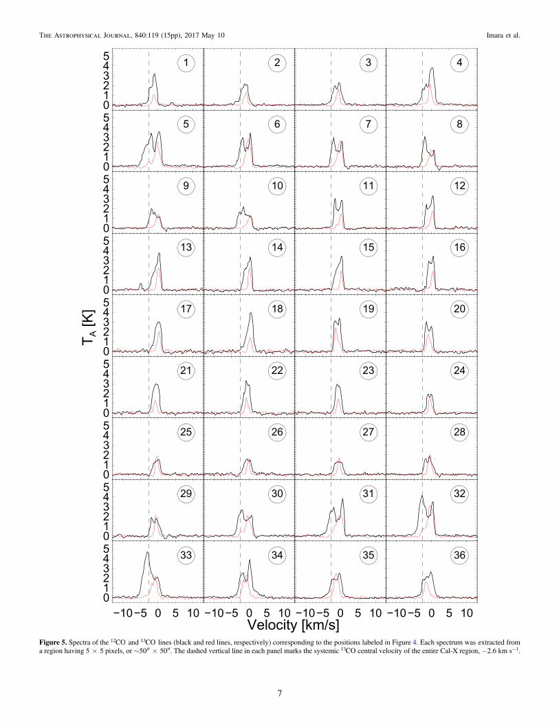
Figure 5. Spectra of the CO12 and CO13 lines (black and red lines, respectively) corresponding to the positions labeled in Figure 4. Each spectrum wasextracted froma region having 5×5 pixels, or ∼50″×50″. The dashed vertical line in each panel marks the systemic CO13 central velocity of the entire Cal-X region, −2.6 -km s 1.

7

The Astrophysical Journal, 840:119 (15pp), 2017 May 10 Imara et al.

uncertainties in the Herschel map and from the uncertainty inthe distance to the California GMC, = d 450 23 pc. We alsoinclude an uncertainty in the gas-to-dust ratio of 10%.

The dust map in Figure 1 reveals the presence of severalcompact, high-extinction subregions embedded throughout Cal-X. We aim to identify cores, keeping two objectives in mind.First, we want to select peaks in the extinction map thatcorrespond to potentially star-forming material. Here we draw onthe argument that cloud material above the extinction of

»A 7.3V mag is most directly related to star formation activity(Lada et al. 2010). This is similar to the threshold for coreformation discussed by André et al. (2010). Second, we want todifferentiate neighboring peaks from each other and from thebackground material. With these criteria, we identify six cores,defined as material enclosed withinbounded contours of

A 7V mag, embedded in SE-fil and SW-fil. Each of thesecores contains a local maximum, i.e., an isolated peak in

emission at a pixel in the map that is not connected to any otherpixels at higher contour levels.Since the cores in the northern region near the outflow are

embedded in gas that has a much higher average extinction thanthe filaments, our criteria for defining their boundaries aresomewhat stricter. In this case, we identify two cores, delineatingtheir boundaries at =A 12V mag. At lower extinctions, the twocores start to blend together, but at 12mag, the cores appear asdistinct local peaks in the extinction map. Contour maps of thetotal of eight cores we define in this way are shown in Figure 8.The selection criteria are somewhat subjective, but theysuccessfully isolate peaks in the extinction map and distinguishneighboring cores from one another. Cores E and F in SW-fil arean exception, in that they appear blended together into onestructure at 7 mag. However, due to the prominent “saddle” inbetween these two local peaks in extinction, we decide to treatthem as distinct objects and measure their properties separately.We compared our results with those of the core extraction

program CLUMPFIND (Williams et al. 1994), an automatedroutine for analyzing hierarchical structure in observations ofmolecular clouds. We used the version of the program for two-dimensional data sets. The algorithm searches for peaks inemission located within a user-defined lowest level contour,and then follows the peaks until all the emission above thedefined threshold can be assigned to specific clumps (Williamset al. 1994). We applied CLUMPFIND to the Herschel dustmap with a range of lowest level contours as inputs, and foundthat at 7 and 12 mag levels, the algorithm extracts the sameeight cores that we identify above.We estimate the effective radius of each core, p=R Aceff ,

from its projected area, Ac, corresponding to continuous pixelshaving extinctions in excess of 7 or 12mag. In calculating thecore masses, to correct for the fact that they are embedded withinregions of high extinction, we perform a background subtractionas follows. For a core having a projected area, Ac, we calculatethe mass within identical background areas having an extinctionof 4 mag, Mback. For each core, we select at least two regions inthe dust map that are near the core without having anyoverlapping emission with it or any other cores. We definethe average mass of these background areas as Mback. Next,we subtract Mback from the uncorrected mass contained withinthe core before subtraction, Muncor. That is, we estimate the coremass as = –M M Muncor back. Similarly, in estimating the numberdensity of a core, we subtract a contribution from its meancolumn density equivalent to =A 4V mag.In Table 3, we list the derived core sizes (ranging from 0.11

to 0.28 pc), the corrected masses (from ∼4 to 88 M ), theuncorrected masses (listed in parentheses), and numberdensities (from ~ ´1.2 104 to ´4.4 104 cm−3).We note that the choice of contouring level effects the

estimated masses, sizes, and other properties of the cores, suchas the virial parameter, which we examine in Section 4. Weperformed additional calculations of the core masses and sizesat = A 7 1V mag and 12±1 mag to get a sense of howmuch the estimates differ. The average core mass at 6 mag is∼1.3 times greater than the estimated average at 7 mag, whichin turn is ∼1.4 times the average at 8 mag. The average coresize at 6 mag is 1.6 times larger than the average size at 7 mag,which is 1.3 times the average size at 8 mag. In Section 4, wewill discuss how the choice in contour level affects estimates ofthe virial parameter.

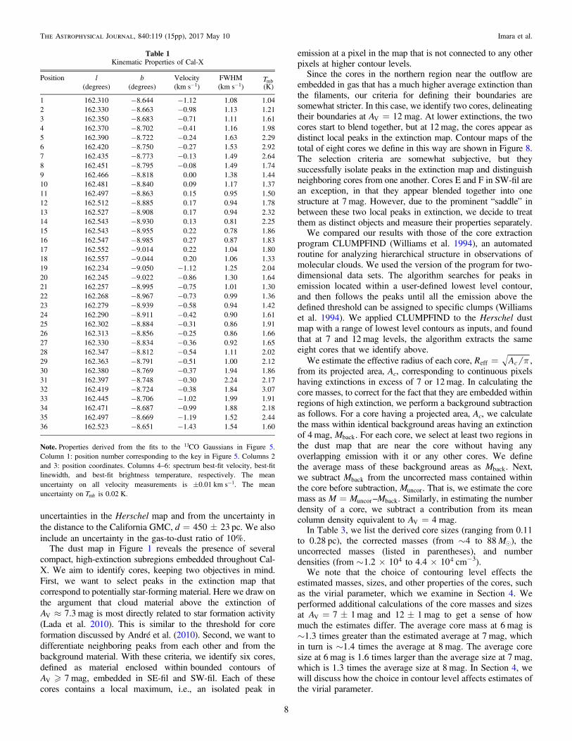
Table 1Kinematic Properties of Cal-X

Position l b Velocity FWHM Tmb(degrees) (degrees) ( -km s 1) ( -km s 1) (K)

1 162.310 −8.644 −1.12 1.08 1.042 162.330 −8.663 −0.98 1.13 1.213 162.350 −8.683 −0.71 1.11 1.614 162.370 −8.702 −0.41 1.16 1.985 162.390 −8.722 −0.24 1.63 2.296 162.420 −8.750 −0.27 1.53 2.927 162.435 −8.773 −0.13 1.49 2.648 162.451 −8.795 −0.08 1.49 1.749 162.466 −8.818 0.00 1.38 1.4410 162.481 −8.840 0.09 1.17 1.3711 162.497 −8.863 0.15 0.95 1.5012 162.512 −8.885 0.17 0.94 1.7813 162.527 −8.908 0.17 0.94 2.3214 162.543 −8.930 0.13 0.81 2.2515 162.543 −8.955 0.22 0.78 1.8616 162.547 −8.985 0.27 0.87 1.8317 162.552 −9.014 0.22 1.04 1.8018 162.557 −9.044 0.20 1.06 1.3319 162.234 −9.050 −1.12 1.25 2.0420 162.245 −9.022 −0.86 1.30 1.6421 162.257 −8.995 −0.75 1.01 1.3022 162.268 −8.967 −0.73 0.99 1.3623 162.279 −8.939 −0.58 0.94 1.4224 162.290 −8.911 −0.42 0.90 1.6125 162.302 −8.884 −0.31 0.86 1.9126 162.313 −8.856 −0.25 0.86 1.6627 162.330 −8.834 −0.36 0.92 1.6528 162.347 −8.812 −0.54 1.11 2.0229 162.363 −8.791 −0.51 1.00 2.1230 162.380 −8.769 −0.37 1.94 1.8631 162.397 −8.748 −0.30 2.24 2.1732 162.419 −8.724 −0.38 1.84 3.0733 162.445 −8.706 −1.02 1.99 1.9134 162.471 −8.687 −0.99 1.88 2.1835 162.497 −8.669 −1.19 1.52 2.4436 162.523 −8.651 −1.43 1.54 1.60

Note. Properties derived from the fits to the CO13 Gaussians in Figure 5.Column 1: position number corresponding to the key in Figure 5. Columns 2and 3: position coordinates. Columns 4–6: spectrum best-fit velocity, best-fitlinewidth, and best-fit brightness temperature, respectively. The meanuncertainty on all velocity measurements is ±0.01 -km s 1. The meanuncertainty on Tmbis 0.02 K.

8

The Astrophysical Journal, 840:119 (15pp), 2017 May 10 Imara et al.

3.4. Infrared Source Properties

The two sources associated with core A(A1 and A2 inFigure 8), were previously identified as YSOs by Harvey et al.(2013) and Broekhoven-Fiene et al. (2014). Broekhoven-Fieneet al. (2014) performed SED modeling on Spitzer observationsof the CMC to determine the YSO classes and physicalproperties, which are summarized in Harvey et al. (2013).Sources A1 and A2, corresponding to source 13 and 12 inHarvey et al. (2013), are located at = - ( ) ( )l b, 162 .47, 8 .68and - ( )162 .46, 8 .68 , respectively. Broekhoven-Fiene et al.(2014) classified source A1 as a class I YSO and determined itsbolometric luminosity to be L0.56 . The authors classified A2as a flat spectrum source with a luminosity of L3.40 . SourceA2 appears prominently in the near-infrared image in Figure 9;in the plane of the sky, it is seen to be projected close to thepeak of the blueshifted lobe of the outflow. Source A1, too faintto be visible in the image, is projected close to the peak of theredshifted lobe of the outflow.

3.5. Outflow

Inspection of the CO12 spectra in the northwest region ofCal-X reveals an excess of emission at high velocitiescompared to other regions. In particular, the CO12 spectra inFigure 5 corresponding to positions 32–36 have surpluses ofblue- and/or redshifted wing emission that suggest a molecularoutflow. However, there are other possible causes for thisexcess emission that must be considered before conclusivelyidentifying the source as an outflow. For instance, the emission

could be due to small background or foreground clouds alongthe line of sight, or it may arise from gas clumps within theCMC that are moving at speeds markedly different from theaverage cloud velocity. Because the presence of excess wingemission is not by itself sufficient to identify an outflow, wefollow Margulis et al. (1988) in adopting more selectivecriteria, which are aided by the contour map and spectrumdisplayed in Figure 9.First, our candidate outflow exhibits bipolarity. Second, the

shape and profile of its average CO12 spectrum departssignificantly from the average spectrum toward Cal-X as awhole, in which most subregions do not display excess emission.Quantitatively, the average CO12 linewidth of Cal-X is3.5 -km s 1, whereas the average spectrum in the vicinity of theoutflow exhibits velocities much greater than (3.5 -km s 1)/2=1.75 -km s 1from the line center. Third, two YSOs are closeto the center of the bipolar outflow candidate and may be itsdriving source. These three criteria are summarized in Figure 9,which shows a near-infrared image of the field containing thesources, created from JHK observations taken at the Calar AltoObservatory in Spain. The image, kindly provided by CarlosRomán-Zúñiga, is overlaid with a contour map of the blue- andredshifted lobes of the outflow, as well as the average CO12

spectrum toward the region in the inset. Only the brighter of thetwo YSOs (A2 in Figure 8) is apparent in the near-infraredimage.To derive the masses of the outflow lobes using the CO12

emission, we first assess the CO12 optical depth. Analysis of theline ratios in Section 3.2 indicates that the CO12 is likely to be

Figure 6. Results of the CO13 spectra fitting (circles) overlaid on the Herschel extinction map. The color and size of the circles represent the gas velocity and the gasvelocity dispersion, respectively.

9

The Astrophysical Journal, 840:119 (15pp), 2017 May 10 Imara et al.

optically thick toward the line center. We estimate the averageratio of line intensities, T T12 13, toward the outflows as afunction of velocity. In the wings, where CO13 emissionbecomes undetectable, we calculate upper limits to the ratio, bysetting the minimum values of T13 to the 1σ rms noise level,0.1 K. We find that the maximum value of T T12 13 toward theoutflow is ∼7, indicating a moderate opacity for the CO12 line.Nevertheless, we estimate the masses of the outflow lobesaccording to the following method, under the assumption thatthe CO12 line is optically thin. Thus, we are likely tounderestimate the optical depth, and therefore the mass.

For each velocity channel in the blue- or redshifted lobe, wecalculate the CO12 optical depth, t12, using

t = - --

⎡⎣⎢

⎤⎦⎥( ) ( )

( ) ( )( )v

T

J T J Tln 1

CO, 312

mb12

ex bg

where = nn -

( )( )

J T h k

h kTexp 1is the radiation temperature

(Rohlfs & Wilson 2004), and ( )T COmb12 , the CO12 main-beam

temperature, depends on velocity. Again, these calculationsassume that the CO12 is optically thin.Next, we assume local thermodynamic equilibrium condi-

tions to estimate the CO12 column density, N12, in each channelusing

òt

= ´ +

´- -

-

( )( )

( )( )

N Tv

Tdv

2.39 10 0.93

1 exp 11.06cm , 4

1214

ex

12

ex

2

where Tex is the excitation temperature, and velocities overwhich we integrate are in units of -km s 1(e.g., Scovilleet al. 1986). For the blueshifted (redshifted) lobe, we integrateover the velocity range of−10 to −4 -km s 1(1–7 -km s 1).Finally, we assume an abundance ratio of = -[ ] [ ]CO H 1012

24

to calculate the total mass per channel,

m=-⎛

⎝⎜⎞⎠⎟

[ ][ ]

( )M m N ACO

H, 5flow H 12 flow

2

1

2

where Aflow is the area of the outflow, mH2 is the mass of anH2molecule, and μ=1.36 is the helium correction factor. Theresulting masses, calculated for three different values of theunknown excitation temperature ( =T 10, 20, 30ex K), arelisted in Table 4. For =T 10ex K, the masses for the blue-and redshifted lobes of the outflow are ∼0.08 and 0.07 M ,respectively.Because the CO12 may not be optically thin, the outflow

masses we determine above are likely to be lower limits. Itwould be preferable to use CO13 to determine the masses, sincethe molecule is more likely to be optically thin. However, whilewe did not detect CO13 toward the outflow, we noted earlier thatthe maximum value ofT T12 13 toward the outflow is∼7. Thus, ifwe assume that =T T 713 12 everywhere in the outflow, we canuse analogous forms of Equations (3) and (4) to calculate t ( )v13and N13 and determine upper limits to the masses. Estimated inthis way, replacing N12 with N13 in Equation (5), and assumingan abundance ratio of = ´ -[ ] [ ]CO H 2 1013

26 (e.g.,

Dickman 1978; Frerking et al. 1982), the masses of the outflowlobes are up to ∼7 times higher than the estimates based on theassumption of optically thin CO12 .

4. Discussion

4.1. Filaments and Cores

The continuous velocity gradients observed along the two Cal-X filaments in Figure 6 might be explained by one of a number ofdifferent processes. The main possibilities are gas inflow(collapse), outflow (expansion), or rotation. Differential rotationseems unlikely, since it would rip apart each filament on the orderof a crossing time. Taking an average 3D velocity dispersion of afilament, s s= » =-( )3 3 0.49 km s 0.843D

1 -km s 1, anda width of∼0.3 pc, we get a crossing time of »t 0.36 Myrcross . IfSE-fil and SW-fil are at least as old as the YSOs in the region,∼1–3Myr, they are probably gravitationally bound or pressureconfined. Since there is no expanding source, such as an H IIregion or molecular outflow, at the nexus of the two filaments, theoutflow scenario also seems unlikely. The molecular outflowassociated with the YSOs is located northward of the filamentsand does not appear to be spatially or dynamically related to them.We therefore suggest that the smooth velocity structure is bestexplained by a global infall of gas toward the center of the system.

Figure 7. Correlations in extinction AV, CO13 peak brightness temperature T13,ratio of CO12 peak brightness temperature to T13, velocity v, and velocitydispersion σ with distance from center of the filaments. Only the error bars forT T12 13 are shown. The typical errors in AV(∼0.02 mag), T13 (∼0.01 K), and vand σ (∼0.005 -km s 1) are smaller than the plot symbols.

10

The Astrophysical Journal, 840:119 (15pp), 2017 May 10 Imara et al.

Considering that the dominant gravitational potential well inCal-X is the high-extinction clump containing the massive cores Aand B, gravity could readily explain the velocity gradients, if allthe gas is falling toward that region. In this scenario, the redshiftedfilament SE-fil is in the foreground, relative to the center of thesystem, while the blueshifted SW-fil is in the background.

To further support the claim of infall, we can useconservation of energy arguments to check whether theobserved velocities along the filaments are consistent withgravitational infall toward the massive clump. A test massstarting from rest at infinity and falling toward a clump of massM and radius R will reach a speed of = ( )v GM R2 1 2 by thetime it arrives at the surface of the clump. In convenientunits, = - -

( ) ( )v M M R0.93 km s 100 pc1 1 2 1 2. We calcu-late this expected v for a range of total clump masses and radiiabove a certain AVthreshold. For 4�AV�13 mag, 9342M963 M , 5R1 pc, and 4v3 -km s 1. Thus,the hypothesis of gravitational infall is plausible since thesevelocities are much larger than the observed velocities alongthe filaments (see Figure 6). It is likely that a confluence ofother physical effects—including external pressures on thefilaments, turbulence, and the fact that the filaments are notpoint masses but extended structures—are working together tooppose gravitational attraction toward the clump, thus slowingdown the infall speeds.

The estimates of the mass-per-unit-lengths of SE-fil and SW-filare, respectively, = M L 54.6 6.8 and -

M65.0 8.4 pc 1.André et al. (2010) suggested that cores can form from filamentsthat have attained the thermal critical mass-per-unit length,

=( )M L c G2 scrit2 (Ostriker 1964), beyond which filaments

are gravitationally unstable. For an∼7K isothermal filament,6 thecorresponding sound speed is m= = -c kT m 0.15 km ss H

12 ,

and = -( )M L M10.4 pccrit

1. The observed values of SE-filand SW-fil are higher by a factor of ∼5–6, suggesting that theyare thermally supercritical. However, magnetic fields may be asource of support against gravitational collapse (Fiege &Pudritz 2000; Beuther et al. 2015; Kirk et al. 2015). In addition,turbulent motions may help stabilize the filaments againstgravity. Following Peretto et al. (2014), we consider an effectivecritical mass-per-unit-length that depends on the averagevelocity dispersion along the filaments, s=( ) ¯M L G2eff

2 .Taking s = -¯ 0.4 km s 1 (see Table 1), we calculate

= -( )M L M74 pceff

1. Since the ratio of the effective to theobserved M/L is ∼0.7–0.9, this suggests that the filaments aresubcritical or, at best, marginally critical. This is equivalent tosaying that the filaments are supported by a gas with an effective

temperature defined by the velocity dispersion:m s =¯m k 53H

22

K. As it turns out, nevertheless, the extinctionmap of Cal-X reveals the presence of a number of overdensestructures.In Section 3.3, we identified eight cores embedded in Cal-X,

six of which are embedded within the filaments SE-fil and SW-fil. In theory, a core is considered to be prestellar if it is starlessand self-gravitating (André et al. 2000; Di Francescoet al. 2007; Könvyes et al. 2015). Such prestellar cores areexpected to develop into protostars. With the exception of coreA, the cores we identified are starless. To assess whether theyare also self-gravitating, we estimate the virial parameter, α, foreach core according to (Bertoldi & McKee 1992)

as

º = ( )M

M

R

GM

5, 6vir

vir2

where Mvir and M are the virial and observed masses of thecore, respectively. An object is self-gravitating if a 2vir

(Bertoldi & McKee 1992). In this way, using the correctedmasses of the cores, we identify core B, with a » 1.5vir , as theonly self-gravitating core. The other cores have virialparameters in the range of3–7 and are therefore likely to bepressure confined. We note that if avir is calculated using theuncorrected masses (i.e., not background-subtracted), we findthat cores A and D are also marginally self-gravitating, witha » 1.9vir for both. The virial analysis may not be valid forcore A, however, since it may be affected by the outflow.As discussed in Section 3.3, the choice of contour level

affects the estimated mass of cores. However, changing theextinction threshold (of 7 and 12 mag) by±1 mag results inonly slight changes to the typical core mass and size, by factorsless than 2. We made additional estimates of the virialparameter using these alternate values of the core mass andsize and found that our results are robust.In their study of a filamentary system composed of three

Spitzer dark clouds, Peretto et al. (2014) similarly conclude thatthe velocity gradients along the filaments are due to infallinggas toward the center of the system where two massive coresare situated. Peretto et al. (2014) decompose this system, calledSDC13, into four filaments, with lengths ranging from 1.6 to2.6 pc, and widths ranging from 0.2 to 0.3 pc, similar to theCal-X filaments. The SDC13 filaments, however, are moremassive (∼195–256 M ) than SE-fil and SW-fil, and theirmass-per-unit-lengths are likely critical or supercritical. Threeof the SDC13 filaments are each embedded with four tofivecores each, whereas the Cal-X filaments have twoandfourcores. Perhaps the greater number of cores in the SDC13filaments are a consequence of them having values of mass-per-unit-length that are closer to supercritical.

Table 2Physical Properties of Filaments

Region Size Mass á ñDensity á ñM L Infall Velocity M(pc×pc) ( M ) ( 104 cm−3) ( M pc−1) ( -km s 1) ( M Myr−1)

Filament East 2.3×0.3 127±16 1.8±0.2 54.6±6.8 0.20 10.7±1.3Filament West 2.4×0.4 154±20 1.6±0.2 65.0±8.4 0.59 38.1±4.9

Note. Properties Calculated for A 4V mag.

6 The typical observed CO12 temperature along the two filaments is»T 3obs K. The corrected temperature from the Rayleigh–Jeans approximation,»T 7cor K, is derived by solving = - -n n

t- n[ ( ) ( )]( )T J T J T 1 eobs cor cmb forTcor, assuming tn 1. n= -n

n( ) ( ) ( )J T h k e 1h kT , and =T 2.725cmb K isthe cosmic microwave background temperature.

11

The Astrophysical Journal, 840:119 (15pp), 2017 May 10 Imara et al.

4.2. Outflow Energetics

Protostellar outflows, particularly in cluster-forming groups,are thought to play a critical role in driving molecular cloudturbulence (Bally et al. 1996; Reipurth & Bally 2001; Knee &Sandell 2000; Maury et al. 2009). How significant is the impacton its surroundings of one outflow driven by a single protostar?In order to investigate the outflow energetics and determine itspossible relationship to turbulence in Cal-X, we estimate theoutflow momentum flux and mechanical luminosity andcompare them to the relevant quantities determined for coreA, with which the outflow is spatially associated. To begin, weuse the CO12 mass estimates of the outflow provided in Table 4to calculate its momentum and kinetic energy,

=

= ( )

P M v

M v

,

KE1

2. 7

flow flow char

flow flow char2

We determine vchar, the characteristic velocity of an outflowlobe, from the intensity-weighted mean absolute velocitysummed over the appropriate velocity range,

å= = å -å

( )∣ ∣( )

( )vv

i N i

T v v v

T vcos

1

cos, 8char

obs

pixels pixels

mb 0

mb

where vobs is the observed velocity and = - -v 2.6 km s01 is the

CO13 systemic velocity of the entire region. In calculatingEquation (8), we assume =v vchar obs. However,since we do notknow the inclination angle i between the line of sight and theflow axis, our estimates of vchar may be underestimated. Forinstance, if i 60 , vchar would be underestimated by as much

as a factor of two. In this way, we calculate the characteristicvelocities of the blueshifted and redshifted outflows to be 3.4and 5.8 -km s 1, respectively. These values, as well as Pflow andKEflow are summarized in Table 5. The total radially directedmomentum of the outflow is 0.67 M -km s 1, implying that bythe time the outflow mass has reached a velocity of1 -km s 1from the line center, it will have swept up0.67 M of material. This is only about ∼0.8% of the massof core A, suggesting that roughly 130 similar generations ofoutflows would be necessary to support core A againstgravitational collapse. How likely is this scenario?Core A appears to be marginally self-gravitating. Based on

its CO13 velocity dispersion and mass, we estimate a » 2.4vir(or, using the uncorrected mass, a » 1.9vir ). To determinewhether the force exerted by the outflow on the core can hinderits collapse, we estimate the momentum flux (or “force”) of theoutflow and compare this to the force required to keep the corein hydrostatic equilibrium. To determine the momentum flux,

=F P tmom flow dyn, we estimate the dynamic timescale of thetwo outflow lobes as =t l vdyn flow char, where lflow is the lengthof a given outflow lobe. We do not consider the inclination i ofthe outflow, but we note that tdyn depends on i via both vchar and

=l l isinflow , where l is the observed projected length on thesky. The projected lengths of the blue- and redshifted lobes areroughly 0.73 and 0.30 pc, respectively, corresponding to

»t 0.2dyn and 0.05Myr. The resulting momentum flux of theblue- and redshifted lobes are 1.4 and -

M7.8 km s 1 Myr−1

(see Table 5). Based on the upper limit estimate of the outflowmass from CO13 observations (see Section 3.5), the totalmomentum flux of the outflow may be up to ∼7 times higher.

Figure 8. Key—locations of cores whose properties are summarized in Table 3.

12

The Astrophysical Journal, 840:119 (15pp), 2017 May 10 Imara et al.

Following Maury et al. (2009), the combined force necessary tobalance gravity at radius R in core A is

p= = ( )F R PGM

R4

2, 9grav

2grav

2

2

where p=P GM R8grav2 4 is the hydrostatic pressure for a

spherical shell of radius R encompassing a mass s=M R G2 2 .Thus, » - -

F M187 km s Myrgrav1 1. The total momentum flux

of the outflow is a factor of ∼20 smaller than Fgrav, suggestingthat the outflow is too weak to provide significant supportagainst collapse in core A. Even if the outflow mass were at theestimated upper limit, the total momentum flux would still beless than Fgrav by a factor of ∼3.

To assess the possible influence of the outflow on turbulencein core A, we approximate the mechanical luminosity of theoutflow, that is, the amount of kinetic energy that it delivers tothe surrounding ISM, using =L tKEmech flow dyn. Not takinginto account inclination, the total mechanical luminosity of theoutflow lobes is ~ ´ -

L4 10 3 . The upper limit is~ ´ -

L28 10 3 . Compared to the 68 molecular outflowscompiled by Lada (1985), who found that Lmech scales withthe luminosity of the driving sources, the outflow and YSOs inCal-X have very low luminosities. We compare this value ofLmech to the rate of turbulent energy dissipation in core A.Following Mac Low (1999) and Maury et al. (2009), we use theone-dimensional CO13 velocity dispersion determined for coreA, s » -1.8 km s 1, to estimate the turbulent energy dissipationrate,

s

s= ( )L

M

R, 10turb

1

22

where = M M84 and R=0.29 pc are the mass and size ofthe core. We find that » L L0.14turb , about a factor of 5–35times greater than the mechanical luminosity of the outflow.These are lower limits, since much of the mechanicalluminosity will be radiated away in shocks. Thus, it appearsthat the outflow is not a dominant contributor to the observedturbulence in the region.

4.3. Origin of Cal-X

The two most massive cores, A and B, located northward ofthe filaments, have a combined mass of ~ M143 . InSection 3.3, we estimated the mass inflow rates of the SE-fil

and SW-fil to be »M 10.7 and 38.1 M Myr−1, respectively.Supposing that the filaments have been funneling gas to themassive cores at a constant rate, and assuming they are themain suppliers of gas to the cores (as opposed to accretion, forexample), it would have taken roughly 2.9Myr for the cores toacquire their current total mass. This is comparable to themedian age of 2±1Myr of YSOs observed in GMCs (e.g.,Covey et al. 2010). It is not obvious, however, whether thefilaments formed before or after the sub-region embedded withthe massive cores or if the regions are coeval. If the filamentsexisted first, then perhaps the present mass of the cores isprimarily due to the infall of gas from the filaments. Thisscenario seems unlikely, though, given that all of the coreswithin SE-fil and SW-fill are starless and only one is self-gravitating, which suggests that the filaments could not be olderthan the region containing the protostars. Thus, we suggest thatthe filaments were born together with or after the massiveregion to the north, which may have attained the bulk of itspresent mass by some mechanism that predated the existence ofthe filaments.In the filament, velocity gradients result from an overall

inflow of mass, and if the cores are moving at the same infallvelocity as the rest of the material in the filaments, then thefilaments may be “raining cores” into the high-mass clump inthe north. In this scenario, based on their observed projecteddistances from the northernmost ends of the filaments, (definedin Section 3.3), the cores in SE-fil and SW-fil may take∼2–5Myr and ∼1–3Myr, respectively, to fall into the high-mass clump. The free-fall times of these cores,

p r=t G3 32ff , are roughly 0.4–0.5 Myr. The “actual”timescale for a core to traverse the length of a filament, treal,depends on the inclination of the filament, as

=t t i icos sinreal obs , where tobs is the timescale estimatedfrom observed filament properties. In order to arrive attimescales as low as the core free-fall times of 0.4–0.5 Myr,the filaments would have to be inclined by at least ∼70°–75°.Thus, unless the filaments are highly inclined with respect toour line of sight, or unless the collapse of these cores is beingslowed by some mechanism such as turbulent support, onemight expect the cores to begin forming stars before (and if)they ultimately “rain” into the high-mass clump.

5. Summary and Conclusions

In this paper, we have presented CO12 (J=2–1) andCO13 (J=2–1) observations of a region of the California

Table 3Physical Properties of Cores

Core ℓ b Reff [Uncorrected] Mass á ñDensity(Degrees) (Degrees) (pc) ( M ) ( 104 cm−3)

A 162.47 −8.69 0.29 [113.4] 84.4±10.9 2.7±0.3B 162.41 −8.72 0.16 [65.3] 58.3±6.9 4.0±0.5C 162.50 −8.86 0.14 [11.6] 6.2±1.4 1.5±0.2D 162.54 −8.92 0.17 [18.2] 10.8±2.3 1.6±0.2E 162.29 −8.90 0.13 [9.9] 5.5±1.2 1.7±0.2F 162.27 −8.95 0.14 [10.7] 5.7±1.3 1.5±0.2G 162.25 −9.02 0.13 [8.4] 4.0±1.0 1.2±0.2H 162.27 −9.05 0.11 [6.8] 3.5±0.8 1.7±0.2

Note. For cores A and B, properties calculated for A 12V mag. For cores C–H, properties calculated for A 7V mag. Column 5 lists the masses of cores afterbackground subtraction, as well as the uncorrected masses, in square brackets, before background subtraction. See Section 3.3.

13

The Astrophysical Journal, 840:119 (15pp), 2017 May 10 Imara et al.

GMC with a low level of star formation activity. Mapped inextinction, this ∼0°.4×0°.6 region (∼3.1 pc× 6.3 pc at thedistance to the CMC) exhibits two prominent filaments, eachjust over 2 pc in length, radiating from a high-column-densityfeature embedded with an outflow driven by one or twoisolated YSOs. Because of its resemblance to an “X” in theextinction map, we dub this region Cal-X. Our main results aresummarized as follows.

1. We examine the CO13 spectra along the filaments and findthat they possess velocity gradients along their lengths,with magnitudes of about 0.1 and - -0.2 km s pc1 1 for thesoutheast and southwest filaments, respectively. Themasses-per-unit-length of SE-fil and SW-fil are, respec-tively, =M L 55 and -

M65 pc 1. This exceeds thecritical thermal mass-per-unit-length, ~ -

M10 pc 1

(assuming a sound speed of 0.095 -km s 1), above whichfilaments become gravitationally unstable (Ostriker 1964).However, if we consider that non-thermal motions maysupport the filaments against gravity, the effective criticalmass-per-unit-length defined by the velocity dispersion ofthe filaments yields = -

( )M L M74 pceff1, suggesting

that the filaments are subcritical or marginally critical.2. Based on the observed coherent velocity structure of the

filaments and their spatial proximity to the large gravita-tional potential well to their north, we suggest that thevelocity gradients are best explained by a northward infallof gas. The combined mass inflow rate of the filamentsis ~ -

M49 pc 1.3. We identify eight cores embedded throughout Cal-X, six

of which are associated with the filaments. The two largest,most massive cores are located in the high-extinctionfeature north of the filaments; one is a starless, prestellarcore; the other is associated with two bright infraredsources. The background-subtracted core masses rangefrom ∼3.5–84 M , and 7 out of 8 of them have virialparameters a = –3 7vir , implying that they are confined bypressure, not gravity.

4. From the CO12 data, we identify a low-velocity, low-massoutflow in the north of Cal-X. The outflow is spatiallycoincident with the highest mass core (84 M ), and it isassociated with the two infrared bright objects that maybe its driving source. The blue- and redshifted lobes ofthe outflow have projected characteristic velocities of 3.4and 5.7 -km s 1, momentum fluxes of 1.4 and

-M7.8 km s 1 Myr−1, and mechanical luminosities of

Figure 9. Near-infrared image of a region of the CMC, created from JHK observations, overlayed with a contour plot of the outflow. The blueshifted (redshifted)emission has been integrated over the velocity range of−10 to −4 -km s 1 (1–7 -km s 1). The contour levels for both blue- and redshifted emission go from 2 to 9

-K km s 1, in steps of 1 -K km s 1. The inset shows the average CO12 spectra toward the entire Cal-X region (solid line) and in the vicinity of the outflow (dashed line).

Table 4Outflow Velocity Ranges and Areas

LobeVelocityRange Area

Mass=[T 10ex K]

Mass=[T 20ex K]

Mass=[T 30ex K]

( -km s 1) (pc2) ( -M10 2 ) ( -

M10 2 ) ( -M10 2 )

Blue −10to −4

0.60 8.3 2.7 1.6

Red 1–7 0.65 6.9 2.2 1.3

Note. Outflow masses for three values of Tex, for the velocity ranges given incolumn 2. The masses are determined from CO12 observations, assuming the

CO12 is optically thin.

14

The Astrophysical Journal, 840:119 (15pp), 2017 May 10 Imara et al.

´ -0.4 10 3 and ´ -L3.6 10 3 . The outflow appears to

be too weak to contribute significantly to the turbulencein the core or to prevent the core from undergoinggravitational collapse.

5. Based on the available observations, we propose that theCal-X filaments were born at the same time or after themassive region to their north, which may have attainedthe bulk of its present mass by some mechanism thatpredated the existence of the filaments. Therefore, giventhe presence of young YSOs in Cal-X, the filaments arelikely to have an age of at least 2±1Myr.

We thank Carlos Román-Zúñiga for providing us with thenear-infrared image in Figure 9. We thank an anonymousreferee and Phil Myers for helpful suggestions that improvedearlier drafts of this paper. The Heinrich Hertz SubmillimeterTelescope is operated by the Arizona Radio Observatory,which is part of Steward Observatory at the University ofArizona, and is supported in part by grants from the NationalScience Foundation. N. Imara is supported by the Harvard-MITFFL Postdoctoral Fellowship.

References

Alves, J., Lada, C. J., & Lada, E. A. 1999, ApJ, 515, 265André, P., Di Francesco, J., Ward-Thompson, D., et al. 2014, in Protostars

and Planets VI, ed. H. Beuther et al. (Tucson, AZ: Univ. Arizona Press), 27André, P., Men’shchikov, A., Bontemps, S., et al. 2010, A&A, 518, L102André, P., Revéret, V., Könyves, V., et al. 2016, A&A, 592, 54André, P., Ward-Thompson, D., Barsony, M., et al. 2000, in Protostars and

Planets IV, ed. V. Mannings, A. P. Boss, & S. S. Russell (Tucson, AZ:Univ. Arizona Press), 59

Andrews, S. M., & Wolk, S. J. 2008, in ASP Monograph Ser. 5, Handbook ofStar-forming Regions, Vol. 2, The Southern Sky, ed. B. Reipurth (SanFrancisco, CA: ASP), 390

Arzoumanian, D., André, P., Didelon, P., et al. 2011, A&A, 529, L6Arzoumanian, D., André, P., Peretto, N., & Könvyes, V. 2013, A&A,

553, A119Bally, J., Devine, D., & Reipurth, B. 1996, ApJ, 473, 49Bertoldi, F., & McKee, C. 1992, ApJ, 395, 140Beuther, H., Ragan, S. E., Johnston, K., et al. 2015, A&A, 584, 67Bieging, J. H., & Peters, W. L. 2011, ApJS, 196, 18Bohlin, R. C., Savage, B. D., & Drake, J. F. 1978, ApJ, 224, 132

Broekhoven-Fiene, H., Matthews, B. C., Harvey, P. M., et al. 2014, ApJ,786, 37

Covey, K. R., Lada, C. J., Román-Zúñiga, C., et al. 2010, ApJ, 722, 971Dickman, R. L. 1978, ApJS, 37, 407Di Francesco, J., Evans, N. J., Caselli, P., et al. 2007, in Protostars and Planets

V, ed. B. Reipurth, D. Jewitt, & K. Keil (Tucson, AZ: Univ. ArizonaPress), 17

Dobashi, K., Uehara, H., Kandori, R., et al. 2005, PASJ, 57, 1Duarte-Cabral, A., Fuller, G. A., Peretto, N., et al. 2010, A&A, 519, A27Fiege, J. D., & Pudritz, R. E. 2000, MNRAS, 311, 85Frerking, M. A., Langer, W. D., & Wilson, R. W. 1982, ApJ, 262, 590Goodman, A. A., Pineda, J. E., & Schnee, S. L. 2009, ApJ, 692, 91Griffin, M. J., Abergel, A., Abreu, A., et al. 2010, A&A, 518, L3Hacar, A., Kainulainen, J., Tafalla, M., Beuther, H., & Alves, J. 2016, A&A,

587, A97Hacar, A., & Tafalla, M. 2011, A&A, 533, A34Harvey, P. M., Fallscheer, C., Ginsburg, A., et al. 2013, ApJ, 764, 133Kirk, H., Klassen, M., Pudritz, R., & Pillsworth, S. 2015, ApJ, 802, 75Kirk, H., Myers, P. C., Bourke, T. L., et al. 2013, ApJ, 766, 115Knee, L. B. G., & Sandell, G. 2000, A&A, 361, 671Kong, S., Lada, C. J., Lada, E. A., et al. 2015, ApJ, 805, 58Könvyes, V., André, P., Men’shchikov, A., et al. 2015, A&A, 584, 91Kutner, M. L., & Ulich, B. L. 1981, ApJ, 250, 341Lada, C. J. 1985, ARA&A, 23, 267Lada, C. J., Lada, E. A., Clemens, D. P., & Bally, J. 1994, ApJ, 429, 694Lada, C. J., Lombardi, M., & Alves, J. F. 2009, ApJ, 703, 52Lada, C. J., Lombardi, M., & Alves, J. F. 2010, ApJ, 724, 687Lombardi, M., Bouy, H., Alves, J., & Lada, C. J. 2014, A&A, 566, 45Lombardi, M., Lada, C. J., & Alves, J. F. 2010, A&A, 512, A67Mac Low, M.-M. 1999, ApJ, 524, 169Margulis, M., Lada, C. J., & Snell, R. L. 1988, ApJ, 333, 316Markwardt, C. B. 2009, in ASP Conf. Ser. 411, Astronomical Data Analysis

Software and Systems XVIII, ed. D. A. Bohlender, D. Durand, & P. Dowler(San Francisco, CA: ASP), 251

Maury, A. J., André, P., & Li, Z.-Y. 2009, A&A, 499, 175Myers, P. C. 2009, ApJ, 700, 1609Ostriker, J. 1964, ApJ, 140, 1056Ott, S. 2010, in ASP Conf. Ser. 434, Astronomical Data Analysis Software and

Systems XIX, ed. Y. Mizumoto, K.-I. Morita, & M. Ohishi (San Francisco,CA: ASP), 139

Peretto, N., Fuller, G. A., André, P., et al. 2014, A&A, 561, A83Reipurth, B., & Bally, J. 2001, ARA&A, 39, 403Rohlfs, K., & Wilson, T. L. 2004, Tools of Radio Astronomy (Berlin: Springer)Schneider, N., Csengeri, T., Hennemann, M., et al. 2012, A&A, 540, 11Scoville, N. Z., Sargent, A. I., Sanders, D. B., et al. 1986, ApJ, 303, 416Ward-Thompson, D., Kirk, J. M., André, P., et al. 2010, A&A, 518, 92Williams, J. P., de Geus, E. J., & Blitz, L. 1994, ApJ, 428, 693Wilson, T. L., & Matteucci, F. 1992, A&ARv, 4, 1

Table 5Outflow Energetics

Lobe vchar Momentum Momentum Flux Kinetic Energy Mechanical Luminosity( -km s 1) ( M -km s 1) ( M -km s 1 Myr−1) (1042 erg) ( -

L10 3 )

Blue 3.4 0.28 1.4 9.6 0.4Red 5.7 0.39 7.8 22 3.6

Note. Energetics of the blue- and redshifted lobes of the outflow.

15

The Astrophysical Journal, 840:119 (15pp), 2017 May 10 Imara et al.