timeseries
TRANSCRIPT

School of Computing, Engineering and Mathematics
TIME SERIES ANALYSIS AND FORECASTING OF THE UK
EXPORT
Khoa Truong
May 2015

Declaration
I declare that no part of the work in this report has been submitted in support of an application
for another degree or qualification at this or any other institute of learning.
Khoa Truong
i

Acknowledgements
First of all, I would like to express my deepest gratitude to my supervisors Dr Alexey Chernov and
Dr Laurie Smith who have given me generous guidance and support till the end of this project. I
am very thankful and grateful to have them as my supervisor and motivational support.
Beside my supervisors, I am highly indebted to all the academic lecturers who have given me an
opportunity to explore mathematics and an unforgettable university experience.
I would like to express my gratitude to my mother who has always been there for me and given
me financial support as well as unequivocal encouragement through out my life, for which, no
matter what and how much I do, it would never be enough to return the favour.
Finally, I am very proud to be a part of Brighton University community. As a student here, I am
very thankful to those sta↵ who has provided me equipments, facilities and services to support in
carrying out this project.
ii

Abstract
Trade performance is considered to be an important element of UK GDP growth of which export
is an essential part. The aim of this paper is to give empirical insight into various forecasting
methods of modelling the UK export series based on time series analysis.
Supervisor: Dr Alexey Chernov
iii
Contents
1 INTRODUCTION 1
1.1 Problem . . . . . . . . . . . . . . . . . . . . . . . . . . . . . . . . . . . . . 1
1.2 Sampling and Series analysis . . . . . . . . . . . . . . . . . . . . . 3
2 THEORETICAL CONTEXT 4
2.1 Univariate time series - linear models . . . . . . . . . . . . . . 5
2.1.1 ARIMA(p,d,q) . . . . . . . . . . . . . . . . . . . . . . . . . . . . . . 5
2.1.2 Dampen component on Exponential smoothing . . . . . . . 6
2.1.3 Linear models summary . . . . . . . . . . . . . . . . . . . . . . . 10
2.2 Univariate time series - nonlinear models . . . . . . . . . . . 10
2.2.1 Introduction to ARCH and GARCH . . . . . . . . . . . . . . . 11
2.3 Multivariate time series analysis . . . . . . . . . . . . . . . . . . 13
2.3.1 Introduction to VARX(p,s) . . . . . . . . . . . . . . . . . . . . . 13
2.4 Forecast Accuracy Instruments . . . . . . . . . . . . . . . . . . . 14
iv
3 LITERATURE REVIEW 16
3.1 UK Popularity Export Forecast Technique . . . . . . . . . . 17
3.2 Existence time series analysis on export application . . 18
4 METHODOLOGY 22
4.1 Export series regression analysis . . . . . . . . . . . . . . . . . . 23
4.2 Models in application . . . . . . . . . . . . . . . . . . . . . . . . . . . 25
4.2.1 Linear regression with Autoregressive errors . . . . . . . . . . 25
4.2.2 VAR(3) and VARX(4,1) . . . . . . . . . . . . . . . . . . . . . . . 30
4.2.3 A(1,1,0), A(0,1,1) and A(1,1,1) . . . . . . . . . . . . . . . . . . 37
4.2.4 Exponential smoothing . . . . . . . . . . . . . . . . . . . . . . . . 44
4.2.5 AR(1)-GARCH(1,2) . . . . . . . . . . . . . . . . . . . . . . . . . . 47
4.2.6 Examing models goodness of fit . . . . . . . . . . . . . . . . . 51
5 FORECAST AND ACCURACY ANALYSIS 52
5.1 Forecast formulation . . . . . . . . . . . . . . . . . . . . . . . . . . . 53
5.2 12 steps ahead forecast accuracy outcomes . . . . . . . . . 55
5.3 Accessing models validation . . . . . . . . . . . . . . . . . . . . . 62
5.3.1 Cross validation . . . . . . . . . . . . . . . . . . . . . . . . . . . . 62
5.3.2 Tracking Signal . . . . . . . . . . . . . . . . . . . . . . . . . . . . . 64
5.3.3 Prediction Interval . . . . . . . . . . . . . . . . . . . . . . . . . . . 67
v
6 LIMITATION AND EXTENSION 70
7 CONCLUSION AND SUGGESTIONS 72
8 EVALUATION 74
9 REFERENCE 75
9.1 Books . . . . . . . . . . . . . . . . . . . . . . . . . . . . . . . . . . . . . . . 75
9.2 Journals . . . . . . . . . . . . . . . . . . . . . . . . . . . . . . . . . . . . . 76
9.3 Websites . . . . . . . . . . . . . . . . . . . . . . . . . . . . . . . . . . . . . 77
9.4 Lecture notes . . . . . . . . . . . . . . . . . . . . . . . . . . . . . . . . . 77
9.5 Thesis . . . . . . . . . . . . . . . . . . . . . . . . . . . . . . . . . . . . . . . 77
9.6 Report . . . . . . . . . . . . . . . . . . . . . . . . . . . . . . . . . . . . . . 78
9.7 Variables and Sources . . . . . . . . . . . . . . . . . . . . . . . . . . 78
10 APPENDIX 79
10.1 Modelling concepts . . . . . . . . . . . . . . . . . . . . . . . . . . . . 79
10.1.1 ACF and PACF . . . . . . . . . . . . . . . . . . . . . . . . . . . . . 79
10.1.2 Stationary Time Series and White Noise . . . . . . . . . . . . 80
10.1.3 Parameter estimator . . . . . . . . . . . . . . . . . . . . . . . . . 80
10.1.4 Model Selection Through Criteria . . . . . . . . . . . . . . . . 80
10.2 SAS Syntax . . . . . . . . . . . . . . . . . . . . . . . . . . . . . . . . . . . 81
vi

List of Figures
1.1 The UK export 14 years export (GBP milion) . . . . . . . . . . . . . . . . . . . 3
2.1 Damp e↵ect on Holt’s model . . . . . . . . . . . . . . . . . . . . . . . . . . . . 8
2.2 Damp a↵ect on Pegels exponential smoothing . . . . . . . . . . . . . . . . . . . 9
3.1 India meat export time series . . . . . . . . . . . . . . . . . . . . . . . . . . . . 19
3.2 Four di↵erent types of rice time series . . . . . . . . . . . . . . . . . . . . . . . 20
3.3 ANN vs exponential smoothing . . . . . . . . . . . . . . . . . . . . . . . . . . . 21
4.1 UK export time series regression analysis . . . . . . . . . . . . . . . . . . . . . . 23
4.2 UK export 95% limits plot . . . . . . . . . . . . . . . . . . . . . . . . . . . . . 24
4.3 UK export time series with outliers removed (red line) . . . . . . . . . . . . . . . 25
4.4 Identify autoregressive for the residuals . . . . . . . . . . . . . . . . . . . . . . . 26
4.5 MLE parameter estimations and model fitness . . . . . . . . . . . . . . . . . . . 26
4.6 Diagostics check for residuals in TR-AR(2) . . . . . . . . . . . . . . . . . . . . . 27
4.7 Export price (index points) . . . . . . . . . . . . . . . . . . . . . . . . . . . . . 28
vii

4.8 Identify autoregressive for the residuals of export against export price . . . . . . 28
4.9 MLE parameter estimations and model fitness . . . . . . . . . . . . . . . . . . . 29
4.10 Diagnostic checks for residuals in PR-AR(2) . . . . . . . . . . . . . . . . . . . . 30
4.11 Residuals diagnostic check . . . . . . . . . . . . . . . . . . . . . . . . . . . . . 31
4.12 Model VAR(3) fitness diagnostics check . . . . . . . . . . . . . . . . . . . . . . 32
4.13 MLE parameter estimates for VAR(3) . . . . . . . . . . . . . . . . . . . . . . . 33
4.14 Exchange rate 1 Pound to USD (left) labour cost (right) . . . . . . . . . . . . . 34
4.15 Identifying rank r and exogenous variable association test . . . . . . . . . . . . . 34
4.16 Model VARX(4,1) fitness diagnostics check . . . . . . . . . . . . . . . . . . . . 35
4.17 MLE parameter estimates for VARX(4,1) . . . . . . . . . . . . . . . . . . . . . . 36
4.18 Correlogram of adjusted UK export series . . . . . . . . . . . . . . . . . . . . . 37
4.19 DF test non-stationary series . . . . . . . . . . . . . . . . . . . . . . . . . . . . 37
4.20 DF test for di↵erenced series . . . . . . . . . . . . . . . . . . . . . . . . . . . . 38
4.21 Correlogram of di↵erences series . . . . . . . . . . . . . . . . . . . . . . . . . . 38
4.22 Maximum likelihood estimations for A(1,1,0) (top), A(0,1,1) (middle), A(1,1,1)
(bottom) . . . . . . . . . . . . . . . . . . . . . . . . . . . . . . . . . . . . . . . 40
4.23 Residuals diagnostic plots (top: normality plots, middle: scatters of residuals,
bottom: corolelograms) for A(1,1,0) . . . . . . . . . . . . . . . . . . . . . . . . 41
4.24 Ljung-Box statistic check residuals for A(1,1,0) . . . . . . . . . . . . . . . . . . 41
4.25 Residuals diagnostic plots (top: normality plots, middle: scatters of residuals,
bottom: corolelograms) for A(0,1,1) . . . . . . . . . . . . . . . . . . . . . . . . 42
viii
4.26 Ljung-Box statistic check residuals for A(0,1,1) . . . . . . . . . . . . . . . . . . 42
4.27 Residuals diagnostic plots (top: normality plots, middle: scatters of residuals,
bottom: corolelograms) for A(1,1,1) . . . . . . . . . . . . . . . . . . . . . . . . 43
4.28 Ljung-Box statistic check residuals for A(1,1,1) . . . . . . . . . . . . . . . . . . 43
4.29 Variation in Tt
from equation (2.9) . . . . . . . . . . . . . . . . . . . . . . . . . 45
4.30 Tt
equation (12) re-modelling using Hot’s winter seasonal . . . . . . . . . . . . 47
4.31 Heteroscedasticity test for the UK export time series . . . . . . . . . . . . . . . 47
4.32 Maximum likelihood parameter estimates and diagnostic check for mean equation
AR(1) . . . . . . . . . . . . . . . . . . . . . . . . . . . . . . . . . . . . . . . . 48
4.33 MLE for parameters and diagnostic check for AR(1)-GARCH(1,2) . . . . . . . . 49
5.1 Export forecast 12 months ahead demonstration . . . . . . . . . . . . . . . . . . 55
5.2 Models’s forecast for export price; VAR(3) (top left), VARX(4,1) (bottom left),
tradingeconomic.com’s model (bottm right) and real export price observations
(top right) . . . . . . . . . . . . . . . . . . . . . . . . . . . . . . . . . . . . . . 59
5.3 Tradingeconomics.com forecast of export (black line) . . . . . . . . . . . . . . . 60
5.4 graphical image of forecast models vs original observations . . . . . . . . . . . . 61
5.5 AR(1)-GARCH(1,2) forecast in 2008 period vs real data . . . . . . . . . . . . . 64
5.6 Tracking signal plot . . . . . . . . . . . . . . . . . . . . . . . . . . . . . . . . . 65
5.7 VARX(4,1) TS for 6 years period in repetition . . . . . . . . . . . . . . . . . . . 66
5.8 Models Prediction intervals . . . . . . . . . . . . . . . . . . . . . . . . . . . . . 68
5.9 AR(1)-GARCH(1,2) predicted volatile . . . . . . . . . . . . . . . . . . . . . . . 69
ix

7.1 VARX(3,1) forecast from Jan-15 to Dec-15 . . . . . . . . . . . . . . . . . . . . 73
x

Acronym Terminology
ARIMA Autoregressive Intergrated Moving Average
ES Exponential Smoothing
DP Damp Pegels
DT Damp Trend
ER Echange Rate
GARCH(p,q) Geralises Autoregressive Conditional Heteroskedasticity order (p,q)
PI Prediction Interval
HW Holt’s Winter
TR-AR(p) Time Regression Autoregressive order p
PR-AR(p) Price Regression Autoregressive order p
TA Trending Adjusted
TS Tracking Signal
VARX(p,s) Vector Autoregressive with Exogenous order p and s
LC Labour Cost
DF Dickey Fuller
ANN Artificial Neuron Network
SBC Schwarz Information Criteria
MLE Maximum Likelihood Estimator
MSE Mean Square Error
MFE Mean Forecast Error
ACF Autocorrelation Function
PACF Partial Autocorrelation Function
Table 1: List of abbreviation
xi

Chapter 1
INTRODUCTION
1.1 Problem
The world population is growing rapidly on a yearly basis and it is expected that demand for goods
will also increase proportionally, which implies that more resources in the UK are required in order
to supply the amount of goods to meet this demand. Ine�cient resource allocation is a factor
that could cause problems to arise as many exporters are unable to predict the uncertainty of the
ever changing commercial market. Nowadays, people can change their choices abruptly and this
can be very unpredictable, presenting one with a degree of uncertainty that can sometimes cause
exporters to miss the requirements of the market within the UK; causing them to misdirect their
supply and waste resources unnecessarily.
In the present, forecasting export o↵ers the means to best improve the decision-making and plan-
ning processes. The ability to forecast will grant firms to estimate and detect any alteration in the
commercial market for products from the UK since supply must meet demand. A well-educated
response to the market based upon statistical analysis will prove to be more profitable than simply
guessing. Meeting the future demand will lead to an increase in export, but access to accurate
forecasting calls for di↵erent methods to be applied on real time data.
1

CHAPTER 1. INTRODUCTION 2
We will explore several statistical methods to discover the optimum model to forecast the UK
export time series, primarily by reviewing various number of popular time series methodology
and claim factors e↵ecting the firms’s ine�cient resource allocation. The paper will go on to
fit the most suitable models to the series and finally analyse the accuracy of the forecasting
techniques. These methods are based on multivariate and univariate linear and non-linear time
series analysis, which have been widely researched to show a good fit. The Non-linear generalises
autoregressive conditional heteroskedasticity of order (1, 2), Regression autoregressive error with
exogenous of order (2) and Vector Autoregressive with exogenous variables order (4,1) have
produced the best forecast for the next 12 months. However to an extent, these models are
invalid in certain circumstances due to its inability to produce a satisfactory forecast, whereas
other models which have produced inaccurate forecasts for the next 12 months appears to pass all
these validations. This will be discussed in-depth and additional information will be comprehend
to support firms decision making and techniques to determine the sustainability of models that can
be employed on an export series; in order to produce the most su�cient and satisfying forecast.
Three measurements have been employed to determine the ”goodness of fit” for the model and
forecast accuracy and they are: MSE (mean square error), MFE (mean forecast error) and MAPE
(mean absolute percentage error).

CHAPTER 1. INTRODUCTION 3
1.2 Sampling and Series analysis
Figure 1.1 is the UK export series plot from the past 14 years spanning the period from January
2000 to December 2014 (measured in million GBP). The series contains a sample of monthly
data of 180 observations. During the period of January 2000 to January 2006 and of January
2009 to December 2014 illustrate the growing was stable within export. There was a high peak
around 2006, which partly relates to the Chinese economic boom, resulting in a huge increase
in shipments of machinery and transport equipment according to Department For International
Development (2011). This had a direct e↵ect on the UK export since its total export accounts
of 40% of machinery (tradingeconomic.com). Up until July 2010, there were two big drops in
export, one in October 2009 and another in July 2007 because of the UK deepest recession in the
history that resulted in huge jobs loss (BBC NEWS (2015)), which was also partly due to the EU
financial crisis. Since EU is the UK’s main export partner, this crisis has left the EU consumer’s
demand to fall, which led to a decline in the UK export. This incident has initiated an unstable
growth period for the UK export business. It is clear to see that the UK export has an upward
non-seasonal trend over the 14 years and does not fluctuate between each month. This shows a
strong relationship between time and UK export, which suggests that time series modelling can
be most appropriate in forecasting the UK export series.
Figure 1.1: The UK export 14 years export (GBP milion)

Chapter 2
THEORETICAL CONTEXT
A time series is a set of data observations varies in time. Time series analysis deals with the
methods of analyzing past data and then projecting the data obtain estimates of future values.
Time Series Analysis have been widely used nowadays especially in financial market such as
Economics variables, stock and exchange rate..etc. This chapter will be a brief description of
time series analysis and theory behind methods of modeling a time series which will be applied
in Chapter 4. Please see appendix for modelling concepts which covering these topics below if
necessary:
• ACF and PACF
• Stationary and white noise
• Parameter estimator: Maximum Likelihood Estimator (MLE)
• Model selection through criteria: Schwarz Information Criteria (SBC)
4

CHAPTER 2. THEORETICAL CONTEXT 5
2.1 Univariate time series - linear models
2.1.1 ARIMA(p,d,q)
For a linear univariate time series popular methods for modelling are Autoregressive (AR), Moving
Average models (MA) and a combination of both ARIMA introduced by Box and Jenkins in 1960.
The general idea of ARIMA(p,d,q) is modelling a stationary time series using the past values of
order p and past error terms of order q and d is the number of di↵erencing required to achieve
stationarity for a time series. The formal mathematical form of the ARIMA(p,d,q) (or often called
A(p,d,q)) model is given below in the form back shift operator:
Zt
= µ+✓(B)
�(B)✏t
, Zt
= (1�B)dyt
(2.1)
where ✓(B) =(1�P
q
q=1 ✓qBq) is a polynomial in B of order q and �(B)= (1�
Pp
p=1 �pBp) is a
polynomial in B of order p. Bnyt
= yt�n
or Bn✏t
= ✏t�n
and if p=q=0 then ✓(B) = �(B) = 1.
✏t
is a white noise process independent and identical distributed (i.i.d), ✏t
s N(0,�2)
Dickey Fuller test
Autocorrelation measures the correlation between some variable yt
, the lagged counterpart yt�1,
period and itself. A stationary time series is a conditional requirement in order to apply ARIMA
modelling, the most common way of detecting stationarity is through the observation of autocor-
relation. What we are looking for is if autocorrelation is decaying to zero exponentially fast or
where most lags lies between standard deviation but this approach is sometimes not appropriate
when dealing with data that is very random and messy. However Mahadeva and Robinson (2014)
have clear demonstrate on a unit root test namely Dickey Fuller test when dealing with messy
data and to help building model, this test following the null hypothesis process where a series can
be assumed to be stationary if it does not have a unit root. Given an AR(1) process:
yt
= � + �yt�1 + ✏
t
The null hypothesis process relies upon the equation coe�cient � where if |�| = 1 then the series
is non stationary and if |�| <1 then the series is in fact stationary. However, the problem here is

CHAPTER 2. THEORETICAL CONTEXT 6
Yt
and Yt�1 under the null hypothesis are non-stationary and when a times series is non-stationary
the normal central limit theorems apply so it is not possible to just readily test on � using an
ordinary t-test. Therefore, by taking Yt�1 from RHS and LHS of the AR(1) equation:
yt
� yt�1 = � + (�� 1)y
t�1 + ✏t
�yt
= � + �yt�1 + ✏
t
Now we have a di↵erenced dependent variable on the LHS and lag 1 on the RHS, so a series
is non-stationary when |�| = 0 and �yt
is then stationary. DF test does not follow a standard
t-distribution so Dickey and Fuller has to tabulate the asymptotic of the distribution. The DF
method is to calculate the t-statistic on � and if t > DF critical value, which then fails to reject
the non-stationarity and thus the method of di↵erencing �yt
has transformed the series to achieve
stationarity.
Extension of AR process
An AR process can be applied to the error term of a Linear Regression model when the residuals are
perceived to be correlated (Tsakiri (2014)). The model can be expressed in a form of regression
with the autoregressive white noise error term:
yt
= �0 + �1x1 + ....+ �i
xi
+ Zt
Zt
=pX
i=1
�p
Zt�p
+ ✏t
, where ✏t
s N(0,�2)
2.1.2 Dampen component on Exponential smoothing
Exponential smoothing arose in the 1950s from the original work of Brown (1962) and Holt
(1960) in time series forecast modelling. Unlike ARIMA exponential smoothing does not require
a stationary time series the method is based on the smoothing process of a series and the forecast
incorporates weighted averages into the methodology. Its method is to decompose the time series
into trend and level in order to predict the future values.

CHAPTER 2. THEORETICAL CONTEXT 7
Damp-Trend Exponential Smoothing (DTES)
DTES is an additive exponential smoothing method as shown below:
Lt
= ↵yt
+ (1� ↵)(Lt�1 + �T
t�1) (2.2)
Tt
= �(Lt
� Lt�1) + (1� �)�T
t�1 (2.3)
yt+h
= Lt
+hX
i=1
�iTt
(2.4)
where Lt
is the level at time t, Tt
is the growth rate at time t and yt+h
is the forecast h step
ahead of time t. An optimum exponential smoothing model (Table 2.1) are mainly depends on
its smoothing parameter 0 ↵ 1 which modifies the time series at each level given time t, 0� 1 trend parameter of time series and 0 � 1 is the autoregressive or the dampen parameter .
Models level trend damping
DT 0 ↵ 1 0< � 1 0< � < 1
Holt 0 ↵ 1 0< � 1 1
Double exponential smoothing (DES) 0< ↵ <1 0< ↵ 1 1
Simple Exponential Smoothing (SES) 0< ↵ < 1 0 0
SES with damped drift 0< ↵ < 1 0 0 < � < 1
SES with drift 0< ↵ < 1 0 1
Random walk with damped drift 1 0 0< � < 1
Random walk with drift 1 0 1
Random walk 1 0 0
Modified exponential smoothing trend 0 0 0< � < 1
Linear Trend 0 0 1
Simple average 0 0 0
Table 2.1: Exponential smoothing models with parameter restrictions
The DTES model has been proven by Flides (2008) with a benchmark that has been di�cult to
beat in empirical studies of forecast accuracy. Holt’s linear exponential smoothing method has
becomes the most popular approach for a trended time series. However, it often found Holt’s
CHAPTER 2. THEORETICAL CONTEXT 8
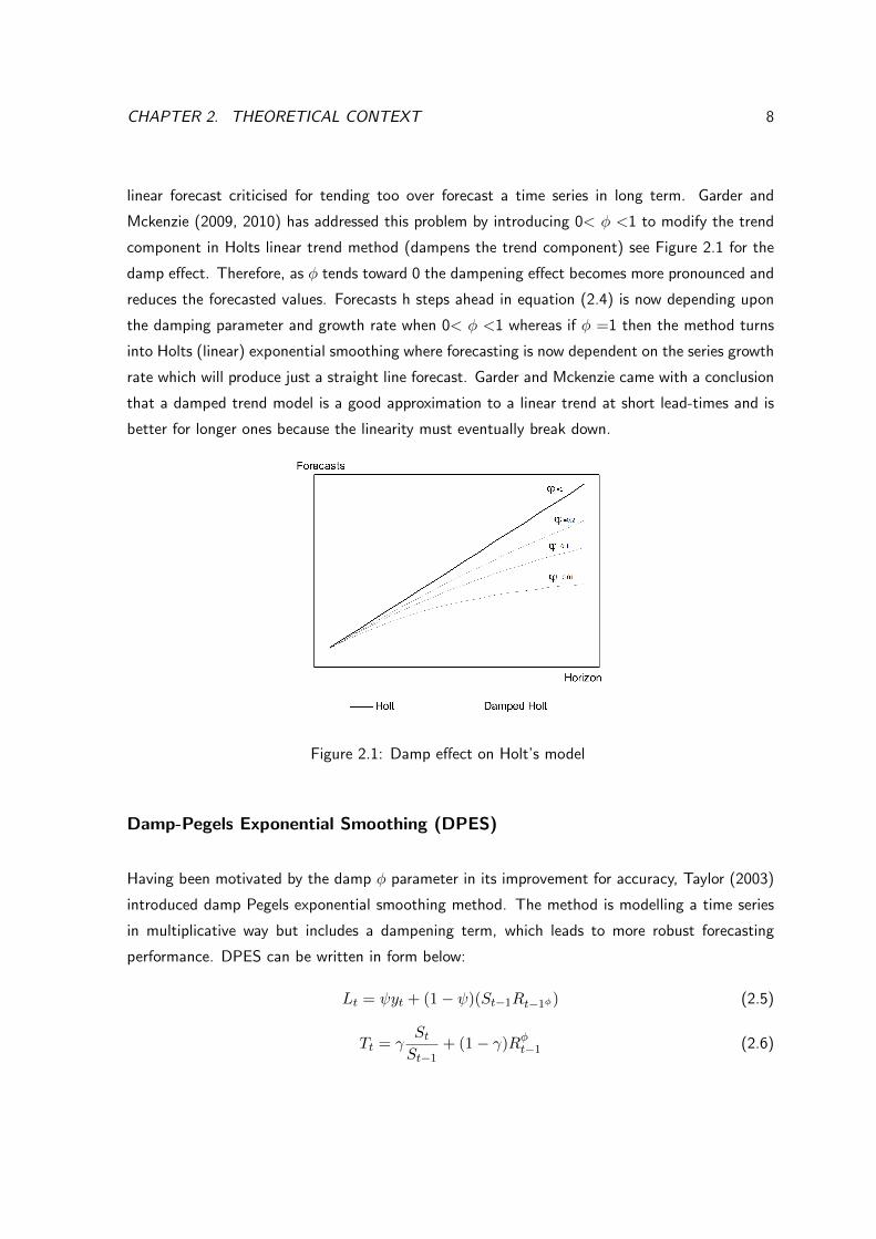
linear forecast criticised for tending too over forecast a time series in long term. Garder and
Mckenzie (2009, 2010) has addressed this problem by introducing 0< � <1 to modify the trend
component in Holts linear trend method (dampens the trend component) see Figure 2.1 for the
damp e↵ect. Therefore, as � tends toward 0 the dampening e↵ect becomes more pronounced and
reduces the forecasted values. Forecasts h steps ahead in equation (2.4) is now depending upon
the damping parameter and growth rate when 0< � <1 whereas if � =1 then the method turns
into Holts (linear) exponential smoothing where forecasting is now dependent on the series growth
rate which will produce just a straight line forecast. Garder and Mckenzie came with a conclusion
that a damped trend model is a good approximation to a linear trend at short lead-times and is
better for longer ones because the linearity must eventually break down.
Figure 2.1: Damp e↵ect on Holt’s model
Damp-Pegels Exponential Smoothing (DPES)
Having been motivated by the damp � parameter in its improvement for accuracy, Taylor (2003)
introduced damp Pegels exponential smoothing method. The method is modelling a time series
in multiplicative way but includes a dampening term, which leads to more robust forecasting
performance. DPES can be written in form below:
Lt
= yt
+ (1� )(St�1R
t�1�) (2.5)
Tt
= �St
St�1
+ (1� �)R�
t�1 (2.6)

CHAPTER 2. THEORETICAL CONTEXT 9
yt+h
= St
RPh
i=1 �i
t
(2.7)
Where Lt
is the level of the time series at time t, St
6= 0 and Tt
denotes the growth rate of
the time series at time t and yt+h
is the forecast h steps ahead. Taylor also has the same view
as Garder and Mckenzie for adding � to PES for believing that PES over forecasts in most of
the time series. If 0 < � < 1, the multiplicative trend is damped and the forecasts approach
an asymptote shown on Figure 2.2 as � tends to 0, the dampened component becomes more
powerful and e↵ectively pulls the forecast down significantly.
Figure 2.2: Damp a↵ect on Pegels exponential smoothing
Trend Adjusted Exponential Smoothing (TAES)
An alternative to Holts and Brown exponential smoothing is TAES. The additive model is given
below:
Ft
= yt�1 + ⇠(y
t�1 � yt�1) (2.8)
Tt
= Tt�1 + �(F
t
� yt�1) (2.9)
yt+h
= Ft
+ hTt
(2.10)
yt+h
is the forecast at a period of h ahead, Ft
is the forecast at time t Tt
is the forecasting trend,
Y is the original observation, yt
is predicted value and ⇠ and � are smoothing parameters. This
model uses both original observations and predicted values for forecasting the model describing a

CHAPTER 2. THEORETICAL CONTEXT 10
trend Tt
as being adjusted for forecasting h step a heads. This special case will be demonstrated
and explained more clearly in the methodology section.
In summary, there is still some limitations with the using ES as it su↵ers from not having an
objective statistical identification and diagnostic system for evaluating the goodness of compet-
ing exponential smoothing models. For example, the smoothing parameters of the models are
determined by fit and are not based on any statistical criteria like tests of hypothesis concerning
parameters or tests for white noise in the errors produced by the model (Fomby, 2008).
2.1.3 Linear models summary
In comparison, ES seems to have the advantage of its procedural simplicity whereas ARIMA models
require many stages of diagnostic checks to achieve a white noise for the error term. Also ES has
the ability to dampen its own trend over a period whereas ARIMA is just a constant projection of
forecasts ahead. Nevertheless, Both ARIMA and exponential smoothing shares similar identities
for example some exponential smoothing methods are shown to be special cases of the class of
Box-Jenkins models (Formby, 2008) and they both are linear predictors. Presumably, for a highly
fluctuate time series, both ARIMA and ES will only give linear forecast values. This sometimes
do not provide su�cient information for firms as uncertainty level is still high since firms may not
know when will be the next turning point? This has becomes problematic since all econometric
series are non-linear with highly fluctuate, this is a complex problem that require a method deals
non-linear time series.
2.2 Univariate time series - nonlinear models
It often found that linearly modelling econometric time series usually leave certain aspects of
economic financial data unexplained. Nevertheless modeling nonlinear time series allow the ex-
istence of di↵erent states of the world or regimes and to allow the dynamics to be di↵erent in
di↵erent regimes. Nonlinear models requires advanced level of understanding in time series as
formulation of these models requires many factors that a↵ects the behavior on a time series. A
very well-known model used by forecasters is artificial/fuzzy neutral network (ANN). This model

CHAPTER 2. THEORETICAL CONTEXT 11
operation is a process where a time series data input into a black box which will be trained using
machine learning technique then produce an output to be the forecast prediction. In applications,
ANN uses is wide spread in stock market, bond ratings, commodity and currency exchange, and
other di�cult-to-predict situations.
2.2.1 Introduction to ARCH and GARCH
An extension from Box and Jenkins models, autoregressive conditional heteroskedasticity (ARCH)
introduced by a Nobel Prize winner Robert F. Engle successfully applied on a non-linear time series.
ARCH has been popular in modelling econometric time series and most famous application on
modeling for stock prices with changing volatility. The term heteroskedasticity refers to unequal
variances on a time series whereas Box Jenkins based on some crucial assumptions, like linearity,
stationarity, and homoscedastic errors. Further more most of econometric time series are often
exhibit features which cannot be explained by linear models. In financial market, less firms choose
to continue to use the linear models as they cannot explain well the behaviour of an econometric
time series satisfactorily, so a model is needed to describe data sets in which variance changes
through time. Given a time series:
Yt
= E(Yt
|⌦t�1) + ✏
t
E(Yt
|⌦t�1) = µ(✓)
Linear models : V ar(Yt
|⌦t�1) = E(✏2
t
|⌦t�1) = �2
ARCH models : V ar(Yt
|⌦t�1) = E(✏2
t
|⌦t�1) = h
t
(✓)
Linear-models gives both conditional, unconditional variance constant (�2) and giving k-step-
ahead forecast error variance depends only on k. Whereas ARCH-models have conditional variance
varies with ⌦t�1 leaving unconditional variance constant and giving k-step-ahead forecast error
variance depends on ⌦t�1. Both linear and ARCH models have conditional mean varies with
⌦t�1. Therefore, ARCH process allows the condition variances to change over time as a function
of squares past errors leaving the unconditional variance constant so it is non-linear in variance
but linear in mean. Besides that, Berra and Higgins (1993) have also explained on other success
of ARCH:

CHAPTER 2. THEORETICAL CONTEXT 12
• ARCH models are simple and easy to handle
• ARCH models take care of clustered errors
• ARCH models take care of nonlinearities
• ARCH models take care of changes in the econometricians ability to forecast
Given an AR(1) process to be the mean equation which have defined in equation (2.1):
yt
= � + �yt�1 + ✏
t
where:
✏t
|⌦t�1 N(0, h
t
)
ARCH(q) process = ht
= ! +qX
i=0
↵i
✏2t�1
where ! > 0,↵i
� 0 for all i andP
q
i=0 ↵i
< 1 are required to be satisfied to ensure non-negativity
and finite unconditional variance of stationary {✏t
} series. The order of lag (q) determines the
length of time for which a shock persists in conditioning the variance of subsequent error. However,
when the order (q) of ARCH model is very large, estimation of a very large number of parameters
(↵) required. To overcome this di�culty, Bolerslev introduced a more general structure in which
the variance model looks more like an ARMA than an AR called generalize ARCH (GARCH) in
which conditional variance is also a linear function of its own lags.
The usual approach to GARCH(p,q) models is to model an error term ✏t
in terms of a standard
white noise et
s N(0, 1) as ✏t
=pht
et
where ht
satisfies the type of recursion used in an ARMA
model:
GARCH(p,q) process = ht
= ! +qX
i=0
↵i
✏2t�i
+pX
j=1
�j
ht�j
(2.11)
A su�cient condition for the conditional variance to be positive is
! > 0,↵i
� 0, i = 1, 2, ...q (2.12)

CHAPTER 2. THEORETICAL CONTEXT 13
�j
� 0, j = 1, 2, .., p (2.13)
The GARCH(p,q) process is weakly stationary if and only if:
qX
i=0
↵i
+pX
j=1
�j
< 1
2.3 Multivariate time series analysis
When two or more variables are influence each other, multivariate time series analysis is most
suitable technique which can explain the interactions and co-movements among a group of time
series. Reason for employing this type of analysis is because future export values are generated
based various factors that e↵ects it.
2.3.1 Introduction to VARX(p,s)
Export is not only contemporaneously correlated to other macroeconomics variables, it also corre-
lated to each others past values. The VARX procedure can be used to model these types of time
relationships. Analyzing and modeling the export and its correlated variable jointly will develop a
better understanding in dynamic relationships between them. Further more, it will also increase
the accuracy of forecasts for each univariate time series by using extra information which available
from the related series and their forecasts. VARX(p,s) (SAS 2014) stands for vector autoregressive
model with exogenous variables. The form of the model can be written as:
yt
=pX
i=1
�i
yt�i
+sX
i=0
⇥⇤i
xt�i
+ ✏t
, where ✏t
s N(0,�2) (2.14)
where dependent variables yt
= (yt
, ..., ykt
)0, t = 1, 2.... denote a k-dimensional time series vector
and xt
= (xt
, ..., xkt
)0 are exogenous variables denote as k-dimensional time series vector. ✏t
=
(✏t
, ..., ✏kt
)0, is a vector white noise process.

CHAPTER 2. THEORETICAL CONTEXT 14
Cointegration
Two time series xt
and yt
are said to be cointegrated if they shares common stochastic drift
process. This means, there exists a parameter � such that Tt
= yt
+ �xt
is a stationary process.
A order of integration, denoted I(d) is minimum number of di↵erences ”d” required to achieve
a stationary time series, a vector of I(1) variables yt
is said to be cointegrated if there exist at
vector �i
such that �0i
yt
is trend stationary. If there exist r such linearly independent vectors
�i
, i = 1, ..., r, then yt
is said to be cointegrated with cointegrating rank r (Bent 2005, p.3). So if
the variables were cointegrated under rank r, we could estimate a Vector Error Correction model
(VECM) instead of transform a nonstationary time series stationary by di↵erencing. A VARX(p,s)
can be represent under Vector Error Correction form below:
�yt
= ⇧yt�1 +
p�1X
i=1
�⇤i
�yt�i
+ADt
+sX
i=0
⇥⇤i
xt�i
+ ✏t
Where ADt
is a constant, ⇧ = �0i
yt
and when ⇧ = 0 implies no cointergration between variables.
Johansen and Juselius proposed the cointegration rank test to determines the linearly independent
columns of ⇧.
2.4 Forecast Accuracy Instruments
Let yt
be h steps ahead predicted value produced by model and yt
be the real observation at time
t+h. Then the error term can be calculated as:
✏t
= yt
� yt
Thus, the model with best forecast accuracy is when ✏t
closest to 0. There has been many
measures of forecast accuracy which have been used in the past and forecasters have made di↵erent
advices about what should be applied when comparing the accuracy of forecast between models.
This section will be discussing some of forecast accuracy measurements in which Hyndman and
Koehler (2005) have suggested to performed well in M and M-3 competition: Mean Square Error
(MSE), Mean Absolute Percentage Error (MAPE) and Mean Forecast Error (MFE):
MFE =
P(y
t
� yt
)
n,MAPE =
P100���yt
� yt
yt
���
n,MSE =
1
n
nX
i=1
(yi
� yi
)2

CHAPTER 2. THEORETICAL CONTEXT 15
Where n is total number of observations. MSE measures whose scale depends on the scale of the
data. These are useful when comparing di↵erent methods on the same set of data, but should
not be used, for example, when comparing across data sets that have di↵erent scales. To address
this MAPE have the advantage of being scale-independent, and so are frequently used to compare
forecast performance across di↵erent data sets. MFE is the measures for bias of errors toward
over and under forecasting i.e if a forecast showing a negative MFE implies the model is over
forecasted.

Chapter 3
LITERATURE REVIEW
This chapter will review various methods of modelling the UK export and their accuracy. Further
more, we will review literature over existence research of time series analysis on exporting and a
brief discussion of forecast accuracy between methods has used in each paper.
16

CHAPTER 3. LITERATURE REVIEW 17
3.1 UK Popularity Export Forecast Technique
The most notable contribution to this literature is a large-scale research in the UK by Dia-
mantopoulos and Winklhofer (2003). This paper provided an insight in popularity forecasting
techniques that firms in the UK like to use in forecasting their export nowadays
The forecasting judgmental techniques incorporate intuitive judgments, opinions and subjective
probability estimates. Delphi method was initially introduced by Olaf Helmer (1962) and the
method has gained popularity in judgmental techniques. According to Helmer (1962, p.1), this
technique employed involves repeated individuals questioning of the experts (by interviews or
questionnaire) and avoid direct confrontation of the expert with one another. The questioning
process requires more than two rounds, experts are expected to provide a summary of their
forecasts and reasons for their judgment from previous round. These forecasts and judgments
will be taken in consideration and then an overall forecast will be produced. Diamantopoulos and
Winklhofer (2003) argued that judgmental forecast techniques are more widely used among firms
compared to statistical technique such as time series, regression. In order to apply successfully
judgmental technique, it requires contextual information which is defined as knowledge gained by
practitioners through experiences on the job, consisting of general forecasting experience in the
industry as well as specific product knowledge. This means that only people holding high position
in a company (i.e. managers, CEO) are able to carry out this task.
Diamantopoulos and Winklhofer surveys 1330 manufacture exporters in the UK to find out their
choice of techniques of forecasting exports. The result showed that 92% percent of the firms
use judgmental techniques and only 8% of statistical technique were employed. They came to
the final conclusion that judgmental technique is more popular amongst surveyed firms. This is
quite surprising as these statistical methods are becoming easy assessable nowadays, for example
computers, software are getting cheaper. There were also some controversies regarding the ap-
propriation of the survey. First, there was only 18% of firms responding to their surveys. Second,
a research reported by Sanders and Manrodt (1994) stated that large firms are more likely to
use statistical techniques due to its cost e�ciency. Therefore, it is insu�cient to conclude that
judgmental techniques are more widely utilized than statically.
Test result found high MAPE values for both judgmental and statistical techniques and for both
CHAPTER 3. LITERATURE REVIEW 18
techniques, short term forecast MAPE is significantly smaller (10%) than long term forecast
(35%). This suggests that short term prediction is significantly more accurate than long term
prediction and of the whole population tested, large proportion of 92% are judgmental technique
which are lies within 10% to 35%. This can conclude that judgmental technique is unreliable
in forecasting accuracy. On the other hand, most firms in UK who employ statistical technique
only for experimental reason is because statistical technique is sometimes unstable in long term
prediction due to a number of discontinuities (i.e it does not take into account of any unexpected
incident) which can only be explained by human judgmental. Therefore combining these two
techniques would produce a better forecasting in export. This paper may open up to an evidence
to why firms in the UK sometimes ine�ciently locate their resources where most of their decision
on how much to supply is based on their own judgment rather than a statistical point of view.
3.2 Existence time series analysis on export application
This section will review four existence research papers and aim to find out the e↵ectiveness of
di↵erent methods of modelling export series:
• Firstly, we will investigate on the e↵ectiveness on ARIMA ”Modelling and Forecasting Meat
Exports from India” carried out by Paul et al (2013).
• Secondly, we will go on review the forecast accuracy of ”Forecasting the Export Prices of
Thai Rice” by Feng et al (2007) using ANN in comparison to ARIMA.
• Thirdly, we will look at ”Forecasting Macroeconomics Variables” (i.e. income, unemploy-
ment rate..etc.) Onder et al (2013) usng ANN and exponential smoothing.
• Finally, we will review ”Forecasting International Trade” by Keck et al (2010) using multi-
variate and univariate time time series analysis.
The meat export time series shows an upward trend multiplicative time series but highly fluctuation
compared to the UK export series shown in Figure 3.1. Paul et al (2013) have successfully applied
a seasonal ARIMA model through ACF and PACF analysis. The model seems to fit well on the
series but in term of forecasting accuracy, seasonal ARIMA is over forecast of MAPE shows only

CHAPTER 3. LITERATURE REVIEW 19
10% error. The reason is that real data compared with the model forecasted values does not
follow the same pattern as the previous year pattern. They could have applied Pegels exponential
smoothing since the data seems to behave multiplicative and exponentially, hence the forecast
trend would look like distortion in between the fluctuations, which may produce a better result.
However the prediction interval for seasonal ARIMA on each month does not vary widely around
the forecasted values and the real observations, therefore the model is still quite adequate. Paul
et al (2013) came to a conclusion that seasonal ARIMA is the best model in modelling the India
meat export.
Figure 3.1: India meat export time series
Feng et al’s (2007) objective is to find an optimum forecast of the weekly Thai rice prices of
four di↵erent types of rice using ARIMA and ANN models. Jasmine and Glutinous rice has no
obvious trend as the time series follows a very random pattern, the rest seems to have an upward
trend and share similar pattern to the UK export time series (figure 3.2 ). The research team
has successfully applied four di↵erent ARIMA models on each category and fitted models are
almost perfect as accuracy estimates MSE, MAPE and others are showing values significantly
close to 0. However, there is a significant change on the forecast accuracy as error estimate
increases significantly in one category, MAPE increased from 0.9876% to 15% errors in glutinous
rice forecast. This is surprising as the past data does not fluctuate that high compared to jasmine
rice. ANN is then applied which act di↵erently to ARIMA as the formulation is to use the time
series data to develop an internal representation of the relationship between the variables, do not
make assumptions about the nature of the distribution of the data and importantly it takes care

CHAPTER 3. LITERATURE REVIEW 20
of non-linearity. The result was significantly improved as MAPE reduces to 11% errors as well
as the reduction in MAPE for other categories. Feng et al (2013) concluded that ANN is better
predictive accuracies.
Figure 3.2: Four di↵erent types of rice time series
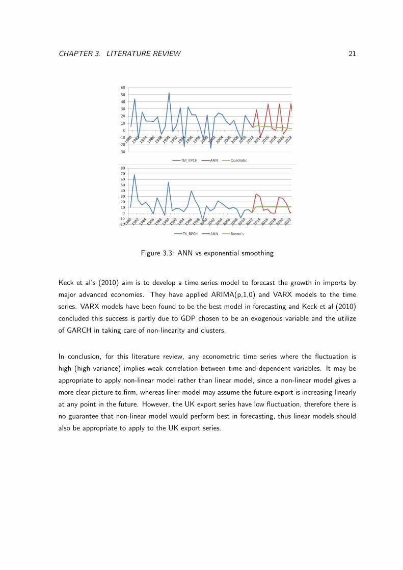
Macroeconomics variables consist of 8 time series and modeling using ANN and exponential
smoothing. All 8 time series behave di↵erently and some of them have very high variance compared
to others. Of the 9 exponential smoothing models applied on these series, Holt’s, Brown’s and
quadratic trend exponential smoothing have shown to have best fit and perform well in the
low variance time series. However, for forecast accuracy, ANN models show a more convincing
results for high variance time series because the way neutral network designed deals of outliers,
high fluctuation and non-linearity produce a more realistic result show in figure 3.3. Exponential
smoothing (green line) prediction is linearly whereas ANN (red line) prediction follows sort of the
past data pattern. The research team came with a conclusion that exponential smoothing only
perform well in short term plus the advantage of their simplicity, whereas ANN might be more
accurate in forecasting but it is too di�cult as there can be infinite number of ways to set up
network. Hence, choosing the right network can become confusing and need some theoretical
knowledge on macro economy.
CHAPTER 3. LITERATURE REVIEW 21
Figure 3.3: ANN vs exponential smoothing
Keck et al’s (2010) aim is to develop a time series model to forecast the growth in imports by
major advanced economies. They have applied ARIMA(p,1,0) and VARX models to the time
series. VARX models have been found to be the best model in forecasting and Keck et al (2010)
concluded this success is partly due to GDP chosen to be an exogenous variable and the utilize
of GARCH in taking care of non-linearity and clusters.
In conclusion, for this literature review, any econometric time series where the fluctuation is
high (high variance) implies weak correlation between time and dependent variables. It may be
appropriate to apply non-linear model rather than linear model, since a non-linear model gives a
more clear picture to firm, whereas liner-model may assume the future export is increasing linearly
at any point in the future. However, the UK export series have low fluctuation, therefore there is
no guarantee that non-linear model would perform best in forecasting, thus linear models should
also be appropriate to apply to the UK export series.

Chapter 4
METHODOLOGY
This chapter will apply Regression with AR errors, ARIMA, ES, GARCH/ARCH and VARX models
to the UK export time series. It was decided to train the data from January 2000 to December
2013 leaving January 2014 to December 2014 to be a hidden data set which will be used later in
chapter 5 to analyses each models forecast accuracy. It will assumes that all calculations, tests
and other statistical diagnostics up to a 95% significant level. The SAS package and SAS (2014)
user’s guide for ARIMA, Autoreg and Varmax procedures are used to compute these models while
Excel is used compute Exponential Smoothing methods. SAS procedures are given in appendix.
22

CHAPTER 4. METHODOLOGY 23
4.1 Export series regression analysis
There has been much debate in the literature regarding what to do with extreme or influential
data points. From Figure 1.1 we can observe that there are few influential data point with high
peak compare to the rest of the data. A simple regression with 95% confident limits is applied
to export series to identify any outliers within the series using SAS procedure [1].
yt
= �0 + �1t+ ✏t
(4.1)
where �0 =19574, �1=143.42301.
Figure 4.1: UK export time series regression analysis
Figure 4.1 Rstudent plot found very few outliers above the 95% limit and very high cook’s distance.
Percentage Residuals histogram shows no obvious skew, which may assume the data is normally
distributed.
In Figure 4.2 below, the 3 outliers are also outside the 95% confident limits although the R-
square is showing a good correlation. Schwager and Margolin (1982) have mentioned the e↵ects

CHAPTER 4. METHODOLOGY 24
Figure 4.2: UK export 95% limits plot
of outliers as it can have serious impact on statistical analysis:
• Firstly, they generally serve to increase error variance and reduce the power of statistical
tests.
• Secondly, if non-randomly distributed they can decrease normality, altering the odds of
making both Type I and Type II errors of the hypothesis test.
• Thirdly, they can seriously bias or influence estimates that may be of substantive interest.
Further more, Section 3.2 have also provided evidence of existence research’s evaluation on e�-
ciency of linear predictors when dealing with a low variance time series, therefore, having outliers
will increase the variance which sometimes misleading the direction of linear predictor to the fu-
ture forecast. In order to overcome all these di�culties, the 3 outliers must be eliminated for a
better forecast result. It was found that these outliers have a relative high peak is in 2006, these
points have identified in Section 1.2 to be the unexpected China and India economy booming
that a↵ected the UK export. Before and after 2006 period, we observed from Figure 4.2 that
the series is growing at a stable rate as all the points are lies in the limits. Therefore it is very
unlikely for the same incident to takes place again and it is 95% confident that the forecast for
the next 12 months will also lies between this limit. Thus these outliers may be considered to be
influential points and linear models would be more su�cient in modelling the UK export without
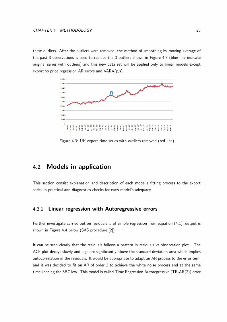
CHAPTER 4. METHODOLOGY 25
these outliers. After the outliers were removed, the method of smoothing by moving average of
the past 3 observations is used to replace the 3 outliers shown in Figure 4.3 (blue line indicate
original series with outliers) and this new data set will be applied only to linear models except
export vs price regression AR errors and VARX(p,s).
Figure 4.3: UK export time series with outliers removed (red line)
4.2 Models in application
This section consist explanation and description of each model’s fitting process to the export
series in practical and diagnostics checks for each model’s adequacy.
4.2.1 Linear regression with Autoregressive errors
Further investigate carried out on residuals ✏t
of simple regression from equation (4.1), output is
shown in Figure 4.4 below (SAS procedure [2]).
It can be seen clearly that the residuals follows a pattern in residuals vs observation plot . The
ACF plot decays slowly and lags are significantly above the standard deviation area which implies
autocorrelation in the residuals. It would be appropriate to adapt an AR process to the error term
and it was decided to fit an AR of order 2 to achieve the white noise process and at the same
time keeping the SBC low. This model is called Time Regression Autoregressive (TR-AR(2)) error

CHAPTER 4. METHODOLOGY 26
Figure 4.4: Identify autoregressive for the residuals
which can be written in the form below:
yt
= �0 + �1t+ Zt
Zt
= �1Zt�1 + �2Zt�2 + ✏t
, Where ✏t
s N(0,�2) (4.2)
Where �0, �1, �1, �2 are the model parameters which shown in SAS output Figure 4.5 below:
Figure 4.5: MLE parameter estimations and model fitness
From Figure 4.5 MLE test for all parameters are significantly < 0.05 which implies these param-
eters are su�cient for TR-AR(2), so parameters below are correspond to Figure 4.5:
�0 = 19843,�1 = 139.0876,�1 = �0.6205,�2 = �0.2814

CHAPTER 4. METHODOLOGY 27
The Durbin-Watson test for positive autocorrelation in residuals found that the p-value>0.05
which fail to reject positive autocorrelation in residuals. Further diagnostic check for this shown
in Figure 4.6, we can observe no significant lags in ACF, no obvious skew in histogram QQ plot
and white noise test shows all lags are below the 5% confident level. Thus we can confirm ✏t
in equation (4.2) to be a white noise. However we can observed few outliers in standardized
residuals which lies outside [-2,2] bound, but not too significant. Further research has carried out
and found no literature to identify these outliers and thus these outliers is retained in this model.
Hence adequacy for TR-AR(2) errors is comfirmed.
Figure 4.6: Diagostics check for residuals in TR-AR(2)
Having motivated by regression model above, further research has found that the general Ex-
port price for goods and services is to be the most fluently variable to the UK export. Export
price contains 168 observations monthly data from Jan 2000 to Dec 2013 and collected from
Tradingeconomic.com shown in Figure 4.7 below

CHAPTER 4. METHODOLOGY 28
Figure 4.7: Export price (index points)
The relationship between export and its price can be easily explained as a negative correlation. This
means export will decrease as its price increase. We can observe this relationship by comparing
Figure 4.7 to figure 1.1 for example during the period from Jan 2000 to Oct 2004 both export and
its price shows to have no movement until 2006 when the price fall leads to export to increase.
Both export and price have been run through SAS to identify autocorrelation in residuals and
output is shown in Figure 4.8 below ((SAS procedure [3]).
Figure 4.8: Identify autoregressive for the residuals of export against export price
We observed from ACF plot that lags are significantly outside standard error area. Again, we can
apply Price Regression AR error order 2 (PR-AR(2)) achieve the white noise process at the same
time keeping SBC stays low. The model equation can be written in form below:
yt
= �0 + �1pricet + Zt
Zt
= �1Zt�1 + �2Zt�2 + ✏t
, where ✏t
s N(0,�2) (4.3)
CHAPTER 4. METHODOLOGY 29
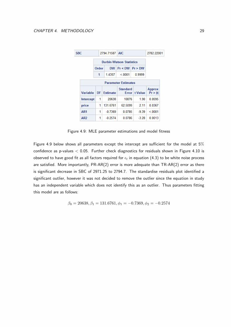
Figure 4.9: MLE parameter estimations and model fitness
Figure 4.9 below shows all parameters except the intercept are su�cient for the model at 5%
confidence as p-values < 0.05. Further check diagnostics for residuals shown in Figure 4.10 is
observed to have good fit as all factors required for ✏t
in equation (4.3) to be white noise process
are satisfied. More importantly, PR-AR(2) error is more adequate than TR-AR(2) error as there
is significant decrease in SBC of 2971.25 to 2794.7. The standardise residuals plot identified a
significant outlier, however it was not decided to remove the outlier since the equation in study
has an independent variable which does not identify this as an outlier. Thus parameters fitting
this model are as follows:
�0 = 20638,�1 = 131.6761,�1 = �0.7369,�2 = �0.2574

CHAPTER 4. METHODOLOGY 30
Figure 4.10: Diagnostic checks for residuals in PR-AR(2)
4.2.2 VAR(3) and VARX(4,1)
VAR(3)
One problem aroused from PR-AR(2) error model as it su↵ered from insu�cient information to
formulate the forecast ahead. This is because export is depending on export price, so without
the forecast ahead for export price it is not possible to carry out the forecast ahead for export.
However, this problem can be solved using VAR modelling 2 dependent variable.
Export and export price have been run through SAS to identify a suitable VAR(p) model and
output are showin in Figure 4.11 below (SAS procedure [4]):

CHAPTER 4. METHODOLOGY 31
Figure 4.11: Residuals diagnostic check
We observed from Figure 4.11 first Table that DF test indicates both series export and its price
are non-stationary with p-value > 0.05. The column Drift in ECM indicates that there is no
separate drift in the error correction model, and the column Drift in Process indicates that the
process has a constant drift before di↵erencing. Fifth column first row on second Table is the
test whether there is cointegrated process in both series at rank 0 (H0 : r = 0), the test show
p-value > 0.05 which cannot be rejected, whereas the test on second row show that there is no
cointegrated process at rank 1 (H0 : r = 1) as p-value <0.05 which reject the null hypothesis.
This implies that export and export price are cointegrated under rank=0. Thus we can fit VAR(p)
model under rank=0 and it was decided to choose p=3 in satisfying the vector white noise process
and lowest SBC. Output are shown in Figure 4.12 (SAS procedure [5]) below and VAR(3) can be
re-written in form of 2 univariate models below:
yexport,(t) = �+�1y
export,(t�1)+�2yexport,(t�2)+�3yexport,(t�3)+✏t, where ✏t
s N(0,�2) (4.4)
yprice,(t) = � + �1y
price,(t�1) + �2yprice,(t�2) + �3y
price,(t�3) + ✏t
, where ✏t
s N(0,�2) (4.5)

CHAPTER 4. METHODOLOGY 32
Figure 4.12: Model VAR(3) fitness diagnostics check
From Figure 4.12 first Table ANOVA diagnostics show that the data is a good fit to the two
univariate models (4.4) and (4.5) as p-value strongly reject the null hypothesis and R-square
very close to 1. We can observed a weak cross correlation of the residuals as all values in cross
correlation of residuals Table are significantly close to zero. In the Univariate model white noise
diagnostics Table:
• The second column shows Durbin Watson values are significantly higher than zero which
implies a strong evidence of uncorrelated in residuals for each univariate model (4.4) and
(4.5)
• The fourth column is the Jarque-Bera normality test show that the residuals are normal for
both univariate model (4.5) and (4.4) as p-value is significantly > 0.05.
• The sixth column test for unequal covariance show that p-value > 0.05 which fails to reject
the null hypothesis meaning each univariate model (4.4) and (4.5) has constant variance.

CHAPTER 4. METHODOLOGY 33
Finally, both (4.4) and (4.5) models AR diagnostics Table shows p-value is significant at 5% level
which implies residuals are uncorrelated in AR 1 to 4. Further more, Portmanteau test for cross
correlations of residuals Table show that p-value is significantly higher than 0.05 from lag 4 to 5
meaning vector error is uncorrelated. Finally, we have su�cient evidence to conclude VAR(3) is
in white noise process.
Figure 4.13: MLE parameter estimates for VAR(3)
We can observe from Figure 4.13 there are some parameters that are insu�cient for this model
as their p-value > 0.05 . However, residuals diagnostic above show the model is good fit and all
these parameters can be retained in this model. The model can be written in vector matrix form
below and parameters �i,(j,k) denote as ARi j k are corresponds to Figure 4.13:
yt
=
�1,(11) �1,(12)
�1,(21) �1,(22)
!yt�1+
�2,(11) �2,(12)
�2,(21) �2,(22)
!yt�2+
�3,(11) �3,(12)
�3,(21) �3,(22)
!yt�3+✏t, ✏t s N(0,�2)
VARX(4,1)
Export price is not the only factor influence export, further research has carried out and found 2
major economics factors that export and its price are mainly depends on are Exchange Rate (ER)
and Labour Cost (LC) shown in Figure 4.14.

CHAPTER 4. METHODOLOGY 34
Figure 4.14: Exchange rate 1 Pound to USD (left) labour cost (right)
These two variables has the same sample size as export and export price which collected from
tradingeconomic.com. Now ER is measuring in USD against 1 Pound and relationship between
export and ER can be described as negative correlation as the Pound gets weaker against USD, this
implies export becomes more a↵ordable and therefore increase the sales in export. LB is measures
in index points and it has negative correlation with export as LB increase will force firms to raise
export price up and leads to decrease in export sales. All variables applied in this model appears
have common stochastic drift, this is shown where each variable has similar peak during 2006 and
similar movement before and after 2006 which indicate the cointeration between these variables.
Causality and cointegration test have been carried out in confirming this association shown in
Figure 4.15 below (SAS procedure [6]):
Figure 4.15: Identifying rank r and exogenous variable association test
The null hypothesis of the Granger causality test is that group 1 variables are influenced only
by itself, and not by group 2. Thus we can clearly observe that p-value is <0.05 which reject

CHAPTER 4. METHODOLOGY 35
the null hypothesis so both export and its price are influenced by LC and ER . Thus we can lag
the exogenous variables by 1, so ”s” = 1. In VAR(3) model we have showed that export and
its price series are non-stationary through DF test. The coinegration test in Figure 4.15 shows
that both series in this case are cointegrated at rank 0 and 1 as their p-values are significantly >
0.05. However it would be more appropriate to model both series under rank 1 as their p-value
is showing a stronger indication of fail to reject the cointegration under rank 1. It was decided
to lag dependent variables by 4 to keep SBC stay lowest at the same time satisfying vector error
to be a white noise, so ”p” = 4. Output for VAR(4,1) diagnostics is shown in Figure 4.16 below
(SAS procedure [7]):
Figure 4.16: Model VARX(4,1) fitness diagnostics check
From Figure 4.16 ANOVA diagnostics show that the data is good fit the two univariate models
export and price as p-value strongly reject the null hypothesis and R-square significantly higher
than 0. However, portmanteau test in the cross correlations of residuals show that p-value is
< 0.05 which reject uncorrelated residuals in cross correlation. Nevertheless, We can observed

CHAPTER 4. METHODOLOGY 36
all tests and statistics from Figure 4.16 show to satisfy white noise process in residuals for both
univariate export and export price models. Also cross correlations of residuals Table show a very
weak cross correlation in the residuals as all values are very close to 0. Thus we may assume that
VARX(4,1) the vector error term is in white noise process and we can comfirm the adequacy for
VARX(4,1). Paramater estiamtes for VARX(4,1) are given in Figure 4.17 below:
Figure 4.17: MLE parameter estimates for VARX(4,1)
The t values and p-values corresponding to the parameters AR1 i j are missing because the
parameters AR1 i j have non-Gaussian distribution (SAS guide). From Figure 4.17, once again
we can retain the parameters for this models despite the MLE test indicates some parameters are
ine�ciency to the model because vector white noise process for VARX(4,1) is satisfied. Note the
D prefixed to a variable name in implies di↵erencing. Thus VARX(4,1) can be written in the
form below:
�yt
=
�1,(11) �1,(12)
�1,(21) �1,(22)
!yt�1 +
�2,(11) �2,(12)
�2,(21) �2,(22)
!�y
t�2 +
�3,(11) �3,(12)
�3,(21) �3,(22)
!�y
t�3
+
�4,(11) �4,(12)
�4,(21) �4,(22)
!�y
t�4 +
⇥⇤
0,(11) ⇥⇤0,(12)
⇥⇤0,(21) ⇥⇤
0,(22)
!xt
+
⇥⇤
1,(11) ⇥⇤1,(12)
⇥⇤1,(21) ⇥⇤
1,(22)
!xt�1 + ✏
t
where ✏t
s N(0,�2)
CHAPTER 4. METHODOLOGY 37
and parameters �i,(j,k) and ⇥⇤
i,(j,k) denote as ARi j k and XLi j k respectively are correspond
to Figure 4.17
4.2.3 A(1,1,0), A(0,1,1) and A(1,1,1)
The Box-Jenkins procedure is concerned with fitting an ARIMA model to data. It has three parts:
identification to see if the data may requires di↵erencing to achieve stationary, estimation to
see if parameter is e�cient for the model and verification to check error term truly is white noise.
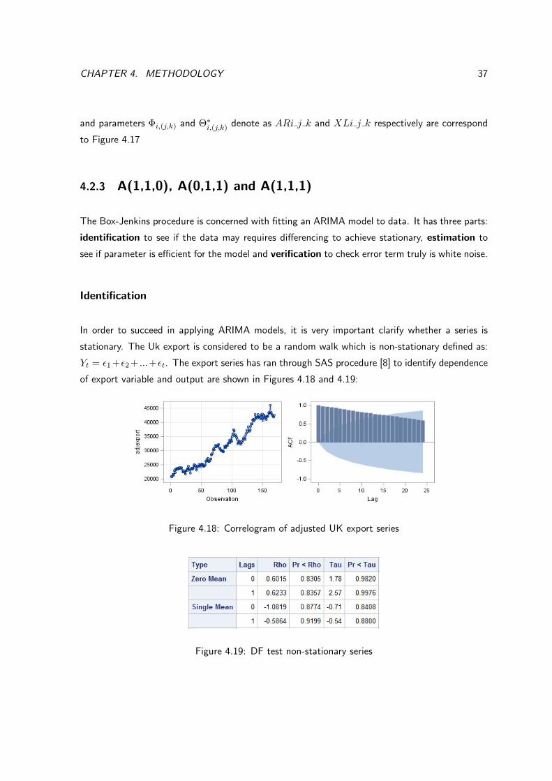
Identification
In order to succeed in applying ARIMA models, it is very important clarify whether a series is
stationary. The Uk export is considered to be a random walk which is non-stationary defined as:
Yt
= ✏1+✏2+ ...+✏t
. The export series has ran through SAS procedure [8] to identify dependence
of export variable and output are shown in Figures 4.18 and 4.19:
Figure 4.18: Correlogram of adjusted UK export series
Figure 4.19: DF test non-stationary series

CHAPTER 4. METHODOLOGY 38
It is clearly to see from Figure 4.18 that lags in AFC plot are significantly above the standard error
area which implies dependent residuals in export variable and that they are not random. ACF is
decay at a very slow rate and the adjexport against time plot on left showing upward trend, it
does not show to have a constant mean and constant variance. DF test has carried out in Figure
4.19, DF test for zero and single mean shows that p-value is significantly > 0.05 which fail to
reject the non-stationary of this time series. Therefore, there is su�cient evidence to show that
the export series is non-stationary, so first di↵erence is required to this series.
Figure 4.20 and 4.21 are SAS output from SAS procedure [9]. Output below is the result after
the first di↵erenced to the export series.
Figure 4.20: DF test for di↵erenced series
Figure 4.21: Correlogram of di↵erences series
The di↵erenced series in Figure 4.21 (adjexport vs observation) plot shows that scatters are varies
constantly around mean of 0. However the variance seems to spread out widely from left to

CHAPTER 4. METHODOLOGY 39
right, so it is not possible to assume variance is constant, this may be due to the time series
is unstable at the at the period after 2006 when the trend grow at a faster rate than before.
Further check on ACF plot in Figure shows that lags are now inside the standard error area and
very close to 0 except lag 1. This indicate the export data set is random and series is stationary.
Further DF has carried out to confirm the series stationarity shown in Figure 4.20. DF test shows
p-value significantly < 0.0001 for both single mean and zero mean implies rejection on the null
hypothesis of non-stationary. Thereby, it is su�cient to conclude the series is stationary. Both
ACF and PACF seems to cut o↵ at lag 1 and unsure which is decay at faster rate, thus this
suggests A(1,1,0), A(0,1,1) and A(1,1,1) can be applied to the series. Thus, the equations (2.1)
above can be written without back shift operator as follows:
A(1, 1, 0) : yt
= � + yt�1 + �y
t�1 + �yt�2 + ✏
t
(4.6)
� = µ(1� �)
A(0, 1, 1) : yt
= µ+ yt�1 � ✓✏
t�1 + ✏t
(4.7)
A(1, 1, 1) : yt
= µ+ yt�1 + �y
t�1 + �yt�2 � ✓✏
t�1 + ✏t
(4.8)
Note all errors term above are i.i.d, ✏t
s N(0,�2)
Estimations
Figures 4.22 below are SAS output of parameter estimations of A(1,1,0), A(0,1,1) and A(1,1,1)
using SAS procedures [10].
Parameters estimates for equations (4.6),(4.7),(4.8) are shown Figure 4.22:
• For (4.6) �=171.977, �=-0.32924
• For (4.7) µ=129.29733, ✓=0.27665
• For (4.8) µ=129.43774, ✓=-0.055, �=-0.37845
MLE output found that t-test for A(1,1,1) have significant p-values > 0.05 for ✓ and �, thus, do
not reject the null hypothesis which implies ✓ = � = 0 in equation (4.8). Whereas A(1,1,0) and

CHAPTER 4. METHODOLOGY 40
A(0,1,1) p-values significantly < 0.05 which implies that ✓ and � are su�cient parameters that
suitable both model in equations (4.6) and (4.7).
Figure 4.22: Maximum likelihood estimations for A(1,1,0) (top), A(0,1,1) (middle), A(1,1,1)
(bottom)

CHAPTER 4. METHODOLOGY 41
Verification
Figures 4.23 to 4.28 below are SAS output of diagnostic check of models A(1,1,0), A(0,1,1) and
A(1,1,1) using SAS procedures [12].
Figure 4.23: Residuals diagnostic plots (top: normality plots, middle: scatters of residuals, bot-
tom: corolelograms) for A(1,1,0)
Figure 4.24: Ljung-Box statistic check residuals for A(1,1,0)
CHAPTER 4. METHODOLOGY 42
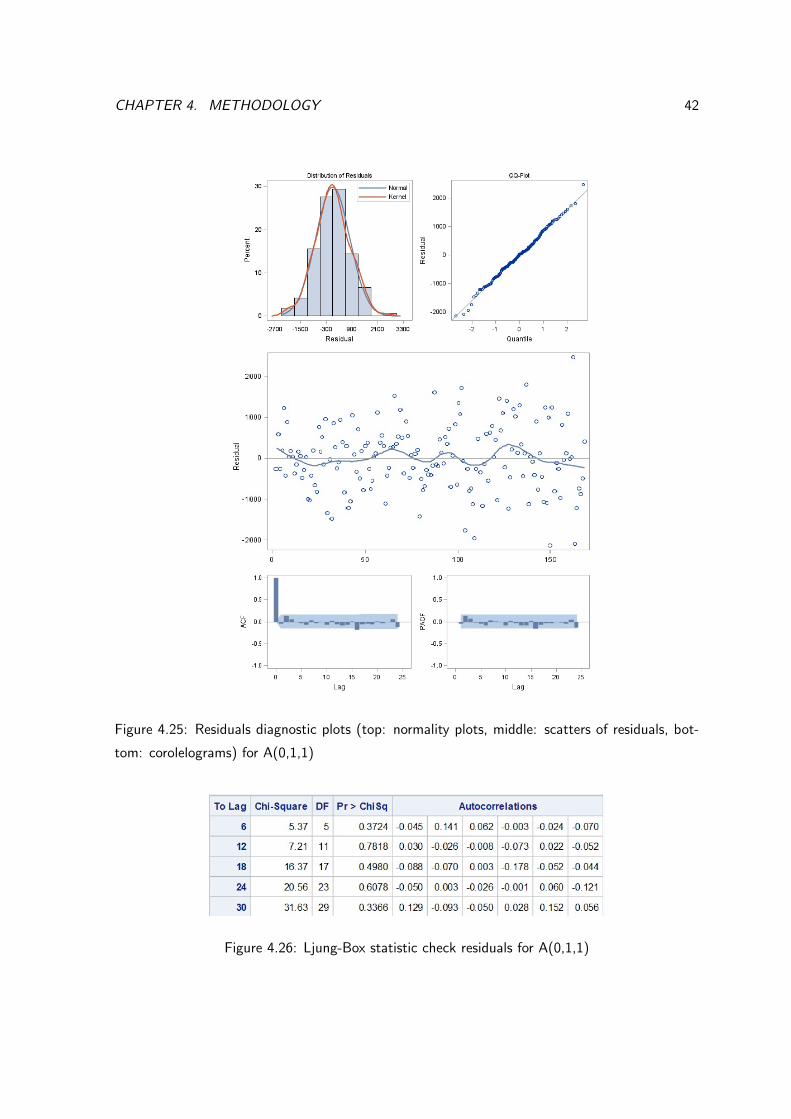
Figure 4.25: Residuals diagnostic plots (top: normality plots, middle: scatters of residuals, bot-
tom: corolelograms) for A(0,1,1)
Figure 4.26: Ljung-Box statistic check residuals for A(0,1,1)

CHAPTER 4. METHODOLOGY 43
Figure 4.27: Residuals diagnostic plots (top: normality plots, middle: scatters of residuals, bot-
tom: corolelograms) for A(1,1,1)
Figure 4.28: Ljung-Box statistic check residuals for A(1,1,1)

CHAPTER 4. METHODOLOGY 44
For the three models in Figure 4.23, 4.25 and 4.27, residuals in QQ plots shows points are lies
close to the fitted line although bottom left and top right has few points slightly o↵ the fitted
line. However, histogram plot shows kernel curves is almost fit the normal curves which appears
to have no obvious skew in the distribution. Scatter plots (residuals vs observation) shows no
obvious pattern, thus it is possible assume that the three linear ARIMA models is appropriate and
that the variance of the residual is constant. ACF for the three models shows no significant lag
outside of standard error area which may be implies residuals are independent. Further Ljuch-box
test is employed to test ✏t
dependency. Figure 4.24, 4.26 and 4.28 shows lags to 30 have p-
values significantly > 0.05, which fail to reject the null hypothesis meaning residuals for A(1,1,0),
A(0,1,1), A(1,1,1) are independent. Now there are su�cient evidence to satisfy the condition for
✏t
to be white noise process. However, despite the failure to reject null hypothesis for A(1,1,1)
parameter test, A(1,1,1) have clearly show to good fit through residuals diagnostics check. We
can conclude that A(1,1,0), A(0,1,1), A(1,1,1) models are adequate for the UK export series.
SBC in Table 4.1 show A(1,1,0) to be the most adequate model with lowest SBC.
Models SBC
A(1,1,0) 2713.700
A(0,1,1) 2716.874
A(1,1,1) 2713.734
Table 4.1: Models comparison
4.2.4 Exponential smoothing
For exponential smoothing DTES, DPES and TAES are most suitable model to satisfy the UK
export time series characteristic. This is because the three methods modelling trend and level
components of a time series. Excel package is mainly used in to perform ES models. To start o↵
with DTES and DPES models, equation Lt
at (2.2),(2.5) and Tt
at (2.3),(2.6) are assumed to be
coe�cient of simple regression model (4.1) where �0 is the intercept which also the level at time
t=0 and �1 is the trend of the fitted regression. Hence, L0= �0= 195.74 and T0=�1=143.42301.
For TAES F0 = first observation = y1 = 20925 and T0 = �1 = 143.423. Smoothing parameters
are obtained by using Excel solver to minimize the value of MSE. The results are shown on Table

CHAPTER 4. METHODOLOGY 45
4.2 below:
Models Parameter estimates damping (�)
holts ↵= 0.726456, � tends to 0 1
DTES ↵=0.7296, � =0.0046335 0.086
DPES = 0.999902 , �= 0.1583 1
DPSE =0.74043 , �= 1 0.0024135
TAES ⇠=0.725899,�=0.00092 n/a
Table 4.2: ES models fitting results
Both models DTES and DPSE shows to have a very strong dampen component, this means the
forecast ahead for holts and PES will be significantly pulled down due to this. All models except
DPSE shows to have a weak trend component where parameter are significantly close to 0. This
implies the level component for each model is one main factor deriving these models and their
forecasts.
Trend adjusted special case
Applying trend adjusted model have given an assess to a clear behaviour of the UK export Tt
in equation (2.9) and this behaviour is shown in Figure 4.29. This method is an attempt in
combining both linear seasonal Holt’s Winter (HW) (Hyndman and Athanasopoulos (2013)) and
non-seasonal method TAES in modelling the UK export.
Figure 4.29: Variation in Tt
from equation (2.9)
CHAPTER 4. METHODOLOGY 46
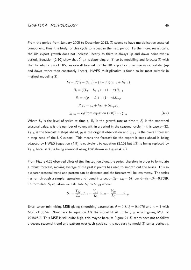
From the period from January 2005 to December 2013, Tt
seems to have multiplicative seasonal
component, thus it is likely for this cycle to repeat in the next period. Furthermore, realistically,
the UK export growth does not increase linearly as there is always up and down point over a
period. Equation (2.10) show that Yt+h
is depending on Tt
so by modelling and forecast Tt
with
the the adaptation of HW, an overall forecast for the UK export can become more realistic (up
and down rather than constantly linear). HWES Multiplicative is found to be most suitable in
method modeling Tt
:
Lt
= #(Yt
� St�p
) + (1� #)(Lt�1 +B
t�1)
Bt
= ⇠(Lt
� Lt�1) + (1� ⇡)B
t�1
St
= (yt
� Lt
) + (1� )St�p
Pt+h
= Lt
+ hBt
+ St�p+h
yt+h
= Ft
(from equation (2.8)) + Pt+h
(4.9)
Where Lt
is the level of series at time t, Bt
is the growth rate at time t, St
is the smoothed
seasonal value, p is the number of values within a period in the seasonal cycle, in this case p=32,
Pt+h
is the forecast h steps ahead, yt
is the original observation and yt+h
is the overall forecast
h step head of the UK export. This means the forecast for the export h steps ahead is being
adapted by HWES (equation (4.9) is equivalent to equation (2.10) but hTt
is being replaced by
Pt+h
because Tt
is being re-model using HW shown in Figure 4.30).
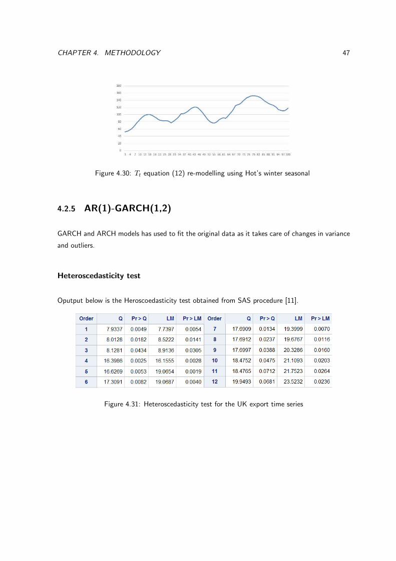
From Figure 4.29 observed allots of tiny fluctuation along the series, therefore in order to formulate
a robust forecast, moving average of the past 6 points has used to smooth out the series. This so
a clearer seasonal trend and pattern can be detected and the forecast will be less messy. The series
has ran through a simple regression and found intercept=�0= L0 = 67, trend=�1=B0=0.7589.
To formulate St
equation we calculate S0 to S�32 where:
S0 =Y32L0
, S�1 =Y31L0
, S�2 =Y30L0
.......S�p
.
Excel solver minimising MSE giving smoothing parameters # = 0.8, ⇠ = 0.4676 and = 1 with
MSE of 83.54. Now back to equation 4.9 the model fitted up to y168 which giving MSE of
794876.7. This MSE is still quite high, this maybe because Figure 24 Tt
series does not to follow
a decent seasonal trend and pattern over each cycle so it is not easy to model Tt
series perfectly.
CHAPTER 4. METHODOLOGY 47
Figure 4.30: Tt
equation (12) re-modelling using Hot’s winter seasonal
4.2.5 AR(1)-GARCH(1,2)
GARCH and ARCH models has used to fit the original data as it takes care of changes in variance
and outliers.
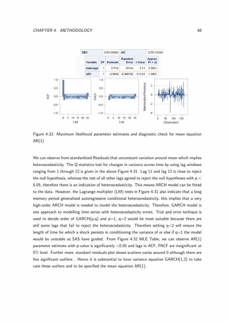
Heteroscedasticity test
Oputput below is the Heroscoedasticity test obtained from SAS procedure [11].
Figure 4.31: Heteroscedasticity test for the UK export time series
CHAPTER 4. METHODOLOGY 48
Figure 4.32: Maximum likelihood parameter estimates and diagnostic check for mean equation
AR(1)
We can observe from standardized Residuals that unconstant variation around mean which implies
heteroscedasticity. The Q statistics test for changes in variance across time by using lag windows
ranging from 1 through 12 is given in the above Figure 4.31. Lag 11 and lag 12 is close to reject
the null hypothesis, whereas the rest of all other lags agreed to reject the null hypotheses with p <
0.05, therefore there is an indication of heteroscedasticity. This means ARCH model can be fitted
to the data. However, the Lagrange multiplier (LM) tests in Figure 4.31 also indicate that a long
memory period generalized autoregressive conditional heteroscedasticity, this implies that a very
high-order ARCH model is needed to model the heteroscedasticity. Therefore, GARCH model is
one approach to modelling time series with heteroscedasticity errors. Trial and error techique is
used to decide order of GARCH(p,q) and p=1, q=2 would be most suitable because there are
still some lags that fail to reject the heteroscedasticity. Therefore setting q=2 will ensure the
length of time for which a shock persists in conditioning the variance of or else if q=1 the model
would be unstable as SAS have guided. From Figure 4.32 MLE Table, we can observe AR(1)
parameter estimate with p-value is significantly <0.05 and lags in ACF, PACF are insignificant at
5% level. Further more, standard residuals plot shows scatters varies around 0 although there are
few significant outliers . Hence it is substantial to have variance equation GARCH(1,2) to take
care these outliers and to be specified the mean equation AR(1).

CHAPTER 4. METHODOLOGY 49
Fitting GARCH(1,2) to AR(1)
SAS procedure [12] fitting GARCH(1,2) to mean equation AR(1) model outputs are shown below
Figure 4.33: MLE for parameters and diagnostic check for AR(1)-GARCH(1,2)
MLE Parameters shows that p-value for ARCH(2) and GARCH(1) = 0.9941 and 0.9421 which
significantly higher 0.05 suggesting the ARCH(2), GARCH(1) is not appropriate. SBC for AR(1)-
GARCH(1,2) is quite close to AR1(1) SBC in Figure 4.32 which implies adding GARCH(1,2) has
little negative e↵ect on its adequacy. However, after fitting GARCH(1,2), standardized residuals
now has only 1 insignificant outlier and varies closer around mean 0 inside the bound [-2,2]. This
shows a better improvement compared to the AR(1) without GARCH(1,2) shown in Figure 4.32
which varies highly outside the [-2,2] bound. Thereby confirming that the mean and variance
equations are correctly specified. AR(1) can be re-written from equation (2.1) without back shift
operator in the form below:
AR(1) = yt
= � + �yt�1 + ✏
t

CHAPTER 4. METHODOLOGY 50
where ✏t
=pht
et
where et
s N(0, 1) and ht
can re-write from equation (2.11) as:
ht
= ! + ↵1✏2t�1 + ↵2✏
2t�2 + �1ht�1 (4.10)
Where:
� = 31717,� = �0.9986,! = 936470,↵1 = 1.1211,↵2 = �0.000785, �1 = 0.000704
All parameters in ht
is su�cient to satisfy the conditional variance to be positive except ↵2 < 0.
However, this wont be such a big problem because ↵2 is very close to 0 so it wont make such
significant e↵ect to the next 12 steps forecast. Also the Bera and Higgin (1993) have pointed
out that from the representation of ht
where:
! > 0,↵i
� 0, i = 1, 2, ..,1
are su�cient to ensure the the conditional variance is strictly positive. Expressing ! and the ↵i
’s
in term of the original parameters of the GARCH model, the condition above does not require
that all the inequalities in (2.12),(2.13) hold. This means for GARCH(1,2) process, ! > 0, ↵1 �0, �1 � 0 �1↵1 + ↵2 � 0 are su�cient to guarantee h
t
> 0 and therefore ↵2 can be negative.
Finally, it is su�cient to conclude that AR(1)-GARCH(1,2) is adequate model for the UK export
time series.

CHAPTER 4. METHODOLOGY 51
4.2.6 Examing models goodness of fit
This section will be discussing performance for each models that have applied in section (5.2).
MSE measurement have employed to analyse each model and the results are shown on Table
below.
Models MSE
A(1,1,0) 627765
A(0,1,1) 639936
A(1,1,1) 627447
TAES 654134
TAES and HWES 794876
holt’s 640541
DT 644360
PES 884793
DPES 670975
TR-AR(2) errors 602894
PR-AR(2) errors 845449
AR(1)-GARCH(1,2) 891740
VAR(3) 987153
VARX(4,1) 833281
Table 4.3: Models goodness of fit
There is a high variation in MSE between models. By far, TR-AR(2) error are best fitted to
the export series with the lowest MSE. Its success is clearly through re-adjusting error term with
AR(2), however, PR-AR(2) error does not perform well in fitness as may due to a significant outlier
in standard residual plot Figure 4.10. ARIMA models are also perform well in their fitness although
A(0,1,1) a little higher. Trending adjusted seems to not fits the data well after being adapted by
HW as the result found a significant increase in MSE from 654134 to 794876. Adaption dampen
parameter (�) shows to have no e↵ect on holt’s models, while dampen parameter added to PES
shows significant reduction in MSE from 884793 to 670975. AR(1)-GARCH(1,2) does not fit well
compared to linear models with the highest MSE.

Chapter 5
FORECAST AND ACCURACY
ANALYSIS
Models with best fit does not means it produces the most accurate forecast, this present chapter
will provide a strong evidence why this is always true. Forecasts produced by each model applied
in Chapter 4 will be fully analysed on its accuracy and validation. All models’ forecasts except
exponential smoothing are computed using SAS, while excel is used for exponential smoothing
52

CHAPTER 5. FORECAST AND ACCURACY ANALYSIS 53
5.1 Forecast formulation
This section will be a brief explanation of each models forecast 12 steps ahead formulations. All
ES models forecast for 12 steps ahead can be computed through their recursion form which will
not be displayed below. for 12 steps ahead forecast, all models below except AR(1)-GARCH(1,2)
has unknown ✏t
which assumed to be 0 and ✏t�1 = y
t�1 � yt�1.
ARIMA(p,d,q)
• A(1,1,0): yt
= � + yt�1 + �y
t�1 + �yt�2
• A(0,1,1): yt
= µ+ yt�1 � ✓(y
t�1 � yt�1)
• A(1,1,1): yt
= µ+ yt�1 + �y
t�1 + �yt�2 � ✓(y
t�1 � yt�1)
Linear regression with AR errors
• TR-AR(2) errors: yt
= �0(1� �1 � �2) + �1[t� �1(t� 1)� �2(t� 2)]
• PR-AR(2) errors: yt
= �1yt�1 + �2yt�2 + �0(1 � �1 � �2) + �1(pricet � �1pricet�1 ��2pricet�2)
VAR(3)
yt+h|t =
�1,(11) �1,(12)
�1,(21) �1,(22)
!yt�1+h|t+
�2,(11) �2,(12)
�2,(21) �2,(22)
!yt�2+h|t+
�3,(11) �3,(12)
�3,(21) �3,(22)
!yt�3+h|t
VAR(4,1)
�yt+h|t =
�1,(11) �1,(12)
�1,(21) �1,(22)
!yt�1+h|t+
�2,(11) �2,(12)
�2,(21) �2,(22)
!�y
t�2+h|t+
�3,(11) �3,(12)
�3,(21) �3,(22)
!�y
t�3+h|t
+
�4,(11) �4,(12)
�4,(21) �4,(22)
!�y
t�4+h|t +
⇥⇤
0,(11) ⇥⇤0,(12)
⇥⇤0,(21) ⇥⇤
0,(22)
!xt+h|t +
⇥⇤
1,(11) ⇥⇤1,(12)
⇥⇤1,(21) ⇥⇤
1,(22)
!xt�1+h|t

CHAPTER 5. FORECAST AND ACCURACY ANALYSIS 54
AR(1)-GARCH(1,2)
Unlike all models above, ✏t
is not assumed to be 0 for h steps ahead. Given AR(1) process:
yt+h
= � + �yt�1 + ✏
t
Let et
= ✏2t
�ht
where E(et
| yt�1)=0. Therefore equation (4.10) can be expressed in form below
(Bera and Higgins 1993 p.317) :
✏2t
= ht
+ et
✏2t
= ! + (↵1 + �1)✏2t�1 + ↵2✏
2t�2 � �1et�1 + e
t
Hence forecast h steps ahead for ✏2t
:
✏2t+h
= ! + (↵1 + �1)✏2t�1+h
+ ↵2✏2t�2+h
� �1et�1+h
+ et+h
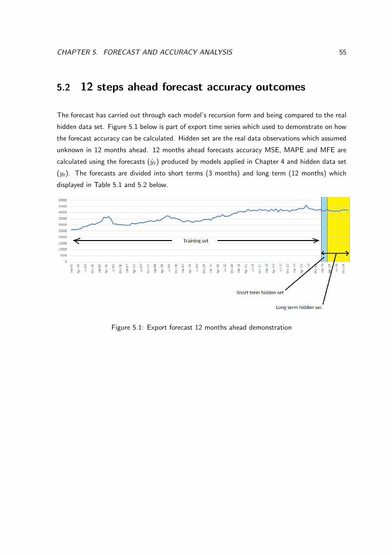
CHAPTER 5. FORECAST AND ACCURACY ANALYSIS 55
5.2 12 steps ahead forecast accuracy outcomes
The forecast has carried out through each model’s recursion form and being compared to the real
hidden data set. Figure 5.1 below is part of export time series which used to demonstrate on how
the forecast accuracy can be calculated. Hidden set are the real data observations which assumed
unknown in 12 months ahead. 12 months ahead forecasts accuracy MSE, MAPE and MFE are
calculated using the forecasts (yt
) produced by models applied in Chapter 4 and hidden data set
(yt
). The forecasts are divided into short terms (3 months) and long term (12 months) which
displayed in Table 5.1 and 5.2 below.
Figure 5.1: Export forecast 12 months ahead demonstration

CHAPTER 5. FORECAST AND ACCURACY ANALYSIS 56
Models MAPE % MSE MFE
A(1,1,0) 2.38 1294951 -988
A(0,1,1) 2.471 1365852 -1021
A(1,1,1) 2.39 1303066 -991
Holt’s 2.55 1427610 -1056
DTES 2.078 949679 -718
PES 2.21 1210405 -884
DPES 2.079 955502 -724
TAES 2.49 1366318 -1028
TAES and HWES 2.39 1306857 -987
TR-AR(2) errors 2.81 1636792 -1166
PR-AR(2) errors 2.86 1618815 -1186
VAR(3) 1.78 705535 -617
AR(1)-GARCH(1,2) 2.027 821829 -597
VARX(4,1) 1.97 678533 -265
Table 5.1: Short term forecasting accuracy results
In short term forecasting, all models performs well at low MAPE and they vary very close together.
The reason for such MAPEs is partly reflects to the behavior of the past data as it does not have
high fluctuate every three months. In particular, VARX(4,1) appears to to be the most accurate
in MSE and MFE. Dampen component has little e↵ect on exponential smoothing methods. It
was a right decision to eliminate the outliers, as result of this have a positive e↵ect on the forecast
accuracy or else the forecast trend could shoot up even more and potentially cause an additional
over forecast.

CHAPTER 5. FORECAST AND ACCURACY ANALYSIS 57
Models MAPE % MSE MFE
A(1,1,0) 3.96 3028581 -1645
A(0,1,1) 4.02 3110772 -1670
A(1,1,1) 3.92 3048664 -1650
Holt’s 4.26 3484090 -1770
DTES 1.98 908244 -809
PES 2.45 1291973 -1009
DPES 2.06 952242 -818
TAES 3.02 1825788 -1252
TAES and HWES 3.81 2814666 -1584
TR-AR(2) errors 4.96 4712094 -2064
PR-AR(2) errors 1.74 611095 -250
VAR(3) 4.26 3484090 -1770
AR(1)-GARCH(1,2) 1.71 762557 -612
VARX(4,1) 1.93 982106 378
Table 5.2: Long term forecasting accuracy results
In long term forecast, similar result to Diamantopoulos and Winklhofer in section 4.1 has found
short term is more accurate than long term but not as significant as Diamantopoulos and Win-
klhofer finding results. Forecast accuracy varies very high between models in the range of 1.7 to
4.26. The model that performs best in long term MAPE is AR(1)-GARCH(1,2), this success is
the result of adapting AR(1) model’s error term by GARCH(1,2) which has successfully captured
the future variance and resulting in a downward trend in the next 12 months shown in Figure (5.4
page 63). This has led AR(1)-GARCH(1,2) to be the most accurate forecast with lowest MAPE.
In fact, it is the only univariate model that is depending on time that is able to predict a down-
ward trend in the 12 months ahead, whereas the forecasts from linear models in Figure 5.4 shows
to never break their upward linearity. Furthermore, this result produced by AR(1)-GARCH(1,2)
support Feng et al (2007) and Onder et al (2013) view (in Section 3.2) on univariate non-linear
models to be more accurate in forecasting compared to linear models.
We observed that dampen component for both PES and Holt’s has contributed significantly to
the forecast accuracy. Dampen component added Holts model has a very robust forecast, this has
e↵ectively increase its forecast accuracy twice from 4.26% to 1.985%. Dampen component added
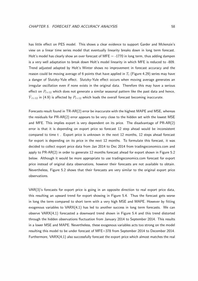
CHAPTER 5. FORECAST AND ACCURACY ANALYSIS 58
has little e↵ect on PES model. This shows a clear evidence to support Garder and Mckenzie’s
view on a linear time series model that eventually linearity breaks down in long term forecast.
Holt’s model has clearly show an over forecast of MFE = -1770 in long term, thus adding dampen
is a very well adaptation to break down Holt’s model linearity in which MFE is reduced to -809.
Trend adjusted adapted by Holt’s Winter shows no improvement in forecast accuracy and the
reason could be moving average of 6 points that have applied in Tt
(Figure 4.29) series may have
a danger of Slutzky-Yule e↵ect. Slutzky-Yule e↵ect occurs when moving average generates an
irregular oscillation even if none exists in the original data. Therefore this may have a serious
e↵ect on Pt+12 which does not generate a similar seasonal pattern like the past data and hence,
Yt+12 in (4.9) is a↵ected by P
t+12 which leads the overall forecast becoming inaccurate.
Forecasts result found in TR-AR(2) error be inaccurate with the highest MAPE and MSE, whereas
the residuals for PR-AR(2) error appears to be very close to the hidden set with the lowest MSE
and MFE. This implies export is very dependent on its price. The disadvantage of PR-AR(2)
error is that it is depending on export price so forecast 12 step ahead would be inconsistent
compared to time t . Export price is unknown in the next 12 months, 12 steps ahead forecast
for export is depending on its price in the next 12 months. To formulate this forecast, it was
decided to collect export price data from Jan 2014 to Dec 2014 from tradingeconomics.com and
apply to PR-AR(2) in order to generate 12 months forecast ahead for export shown in Figure 5.2
below. Although it would be more appropriate to use tradingeconomics.com forecast for export
price instead of original data observations, however their forecasts are not available to obtain.
Nevertheless, Figure 5.2 shows that their forecasts are very similar to the original export price
observations.
VAR(3)’s forecasts for export price is going in an opposite direction to real export price data,
this resulting an upward trend for export showing in Figure 5.4. Thus the forecast gets worse
in long the term compared to short term with a very high MSE and MAPE. However by fitting
exogenous variables to VARX(4,1) has led to another success in long term forecasts. We can
observe VARX(4,1) forecasted a downward trend shown in Figure 5.4 and this trend distorted
through the hidden observations fluctuation from January 2014 to September 2014. This results
in a lower MSE and MAPE. Nevertheless, these exogenous variables acts too strong on the model
resulting this model to be under forecast of MFE=378 from September 2014 to December 2014.
Furthermore, VARX(4,1) also successfully forecast the export price which almost matches the real

CHAPTER 5. FORECAST AND ACCURACY ANALYSIS 59
observations of export price shown in Figure 5.2. However this raises controversy of the relationship
between export and its price as VARX(4,1)’s forecast trend shows a positive correlation between
both export and its price, but this is not true in the financial world.
Figure 5.2: Models’s forecast for export price; VAR(3) (top left), VARX(4,1) (bottom left),
tradingeconomic.com’s model (bottm right) and real export price observations (top right)
Although ARIMA and TR-AR(2) error have performed very well in term of goodness of fit in
section (5.3) and yet their forecast is till far from accurate compared to other models according
to Table 6.
In Figure 5.3 it can be observed that the forecast carried out by Tradingeconomics.com for
the same 12 months ahead which shows to be more accurate as their forecasts are close/in-
between the hidden data set trend in a parabola shape, whereas all models applied in this project
appear to be over forecasted with high negative MFE. AR(1)-GARCH(1,2) and PR-AR(2) error
have similar downward trend forecast up until October 2014 but at a slower rate compared to
tradingeconomics.com’s model, VARX(4,1) has the same downward trend as the original data
trend up until mid-August. Tradingconomic.com have also applied ARIMA models, but reason
for their success is that they have calibrated using their analysts expectations combine with
complex process of adjusting the coe�cients of the econometric model by taking into account
their analysts assessments and future expectations. This means they have taken into account
various number of factors e↵ecting the UK export in order to produce an e�cient forecast.

CHAPTER 5. FORECAST AND ACCURACY ANALYSIS 60
Figure 5.3: Tradingeconomics.com forecast of export (black line)

CHAPTER 5. FORECAST AND ACCURACY ANALYSIS 61
Figure 5.4: graphical image of forecast models vs original observations

CHAPTER 5. FORECAST AND ACCURACY ANALYSIS 62
5.3 Accessing models validation
Two Section (6.1) have clearly show AR(1)-GARCH(1,2) PR-AR(2) errors and VARX(4,1) perform
very well in accuracy of 12 steps ahead. However is it always the case? The following points
was raised by Hyndman (2013) on the e�ciency of modelling time series and their satisfactory
forecasts:
• A model which fits the data well does not necessarily forecast well.
• A perfect fit can always be obtained by using a model with enough parameters.
• Over-fitting a model to data is as bad as failing to identify the systematic pattern in the
data.
Further investigation have carried out in this section in comparing each model validation and
to see whether these models are working e�ciently in order to produce a satisfy forecast. T
techniques have employed: Cross validation, Tracking Signal (TS) and Prediction Interval (PI) to
judge on a model validation.
5.3.1 Cross validation
Cross validation (Hyndman (2005)) is a repetition of modelling and forecast a data set at di↵erent
time location. The data will be divided into 2 data sets: training set and hidden set. A forecast
is produced through modelling training set and the hidden set is a future observations which we
assume its unknown. The process of cross validation is a repetition of Section 4 and 5.2 but at
di↵erent time t. Cross validation procedures and results are shown below:
1. Fit models to a training set which will be a set a data from Jan-2000 to Dec-2007
2. Produce the forecast accuracy from step 1 by calculating MSE against hidden set of 12
months from Jan 2008 to Dec 2008
3. Repeat the same procedures until the last hidden set is the period from Jan 2013 to Dec
2013

CHAPTER 5. FORECAST AND ACCURACY ANALYSIS 63
Models 2008 2009 2010 2011 2012 2013 average
A(1,1,0) 3156082 2704885 4123895 1736159 2792451 1571797 2680878
A(0,1,1) 3199304 2775024 4136711 1794194 2874733 1550414 2721730
A(1,1,1) 3158083 2652229 4121848 1714857 2775148 1570340 2665417
Holt’s 4348612 4981301 3516347 2298361 3849669 4798425 3965452
Damped-trend 4021644 3348751 2846133 2124631 2487968 4021432 2808426
PES 3311861 5446314 3556849 1564879 3046686 4456320 3563818
damped PES 3165463 4268035 2325146 2251361 2786963 3216431 3002233
TA 4315563 2531463 3833462 3678461 1378643 4433421 3361835
TR AR(2) errors 4315126 3206862 2856891 5525366 786163 1529008 3036569
PR AR(2) error 11395299 937722 9416091 4493399 522121 2202621 4827875
VAR(3) 2770668 3182447 3646483 2444489 1530276 1608813 2530529
VARX(4,1) 2508567 1829908 854731 2578669 922503 1682510 1729481
AR(1)-GARCH(1,2) 7568315 1504604 1237379 6651685 575203 2604712 3356983
Table 5.3: Six di↵erent years forecast accuracy in MSE
ARIMA and VAR(3) models might have not perform well in Section 5 but di↵erent results are
found from Table 8 as we observed that their forecast accuracy are consistent throughout the 6
periods and they have average MSE lower than ES models. In particular VAR(3) has successfully
show a strong relationships between export and its price varies in 6 training period. Flides proof
in Section 2.1.2 on damp trend to be best in forecast accuracy is not true in this case although its
MSE is quite close to ARIMA. However, once again, the result of training data has also agreed with
Gardner and McKenzie’s conclusion adding dampen parameter on improving forecast accuracy.
As the result, MSE decreased significantly on both damped-trend and damped PES throughout
the 6 training periods. It is not possible carried out HWES on TAES due to insu�cient seasonal
components so no conclusion can be made on its forecast accuracy, although TAES itself is still
performing well on average. We observe very high average MSE for PR-AR(2) error model which
raises a controversial point that has been made in Section 5.2 about export’s dependency on price,
thus these training results truly show that export does not depend much on its price throughout
the 6 training period, but it is dependent more on time as TR-AR(2) error has significantly
lower average MSE. AR(1)-GARCH(1,2) model show to have inconsistent accuracy throughout
6 training periods. We observed AR(1)-GARCH(1,2) in 2009, 2010 and 2012 has very low MSE
compare to the rest. It is unsure the reason for such high average MSE but it is partly related
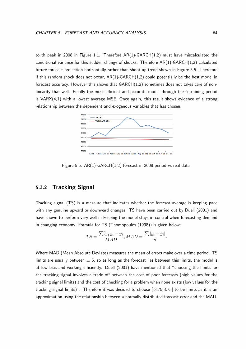
CHAPTER 5. FORECAST AND ACCURACY ANALYSIS 64
to th peak in 2008 in Figure 1.1. Therefore AR(1)-GARCH(1,2) must have miscalculated the
conditional variance for this sudden change of shocks. Therefore AR(1)-GARCH(1,2) calculated
future forecast projection horizontally rather than shoot up trend shown in Figure 5.5. Therefore
if this random shock does not occur, AR(1)-GARCH(1,2) could potentially be the best model in
forecast accuracy. However this shows that GARCH(1,2) sometimes does not takes care of non-
linearity that well. Finally the most e�cient and accurate model through the 6 training period
is VARX(4,1) with a lowest average MSE. Once again, this result shows evidence of a strong
relationship between the dependent and exogenous variables that has chosen.
Figure 5.5: AR(1)-GARCH(1,2) forecast in 2008 period vs real data
5.3.2 Tracking Signal
Tracking signal (TS) is a measure that indicates whether the forecast average is keeping pace
with any genuine upward or downward changes. TS have been carried out by Duell (2001) and
have shown to perform very well in keeping the model stays in control when forecasting demand
in changing economy. Formula for TS (Thomopoulos (1998)) is given below:
TS =
Pn
t=1 yt � yt
MAD,MAD =
P|y
t
� yt
|n
.
Where MAD (Mean Absolute Deviate) measures the mean of errors make over a time period. TS
limits are usually between ± 5, so as long as the forecast lies between this limits, the model is
at low bias and working e�ciently. Duell (2001) have mentioned that ”choosing the limits for
the tracking signal involves a trade o↵ between the cost of poor forecasts (high values for the
tracking signal limits) and the cost of checking for a problem when none exists (low values for the
tracking signal limits)”. Therefore it was decided to choose [-3.75,3.75] to be limits as it is an
approximation using the relationship between a normally distributed forecast error and the MAD.

CHAPTER 5. FORECAST AND ACCURACY ANALYSIS 65
Result are shown in table 7 and Figure 5.6 below. Note that ARIMA, TAES with and without
HWES, holt’s with and without damp, PES with and without damp, TR-AR(2) error models and
VAR(3) are denotes under BIAS is group because they have same TS.
dates BIAS AR(1)-GARCH(1,2) PR-AR(2) error VARX(4,1)
Jan-14 -1 -1 -1 -1
Feb-14 -2 -2 -2 -2
Mar-14 -3 -2.5 -2.13 -0.97
Apr-14 -4 -3.55 -3.12 -1.55
May-14 -5 -4.541 -4.07 -1.99
Jun-14 -6 -5.574 -5.11 -2.85
Jul-14 -7 -6.558 -6.02 -2.51
Aug-14 -8 -7.583 -7.06 -3.22
Sep-14 -9 -8.539 -7.29 -0.72
Oct-14 -10 -9.207 -6.44 1.77
Nov-14 -11 -9.794 -5.37 3.83
Dec-14 -12 -10.396 -4.14 5.60
Table 5.4: Tracking signals data
Figure 5.6: Tracking signal plot
We observed from Figure 5.6, all models except VARX(4,1) are out of control in long term as
their forecast fall out of limits, whereas in short term period which up to April all models are
perfectly in control. In comparison, BIAS group of models forecast are too robust compare to
the rest resulting the models with high bias. Therefore, these models should be modified (i.e
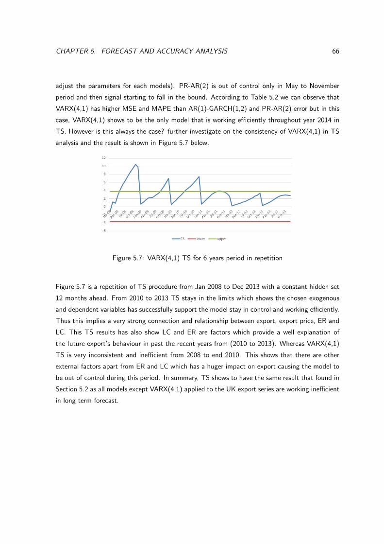
CHAPTER 5. FORECAST AND ACCURACY ANALYSIS 66
adjust the parameters for each models). PR-AR(2) is out of control only in May to November
period and then signal starting to fall in the bound. According to Table 5.2 we can observe that
VARX(4,1) has higher MSE and MAPE than AR(1)-GARCH(1,2) and PR-AR(2) error but in this
case, VARX(4,1) shows to be the only model that is working e�ciently throughout year 2014 in
TS. However is this always the case? further investigate on the consistency of VARX(4,1) in TS
analysis and the result is shown in Figure 5.7 below.
Figure 5.7: VARX(4,1) TS for 6 years period in repetition
Figure 5.7 is a repetition of TS procedure from Jan 2008 to Dec 2013 with a constant hidden set
12 months ahead. From 2010 to 2013 TS stays in the limits which shows the chosen exogenous
and dependent variables has successfully support the model stay in control and working e�ciently.
Thus this implies a very strong connection and relationship between export, export price, ER and
LC. This TS results has also show LC and ER are factors which provide a well explanation of
the future export’s behaviour in past the recent years from (2010 to 2013). Whereas VARX(4,1)
TS is very inconsistent and ine�cient from 2008 to end 2010. This shows that there are other
external factors apart from ER and LC which has a huger impact on export causing the model to
be out of control during this period. In summary, TS shows to have the same result that found in
Section 5.2 as all models except VARX(4,1) applied to the UK export series are working ine�cient
in long term forecast.

CHAPTER 5. FORECAST AND ACCURACY ANALYSIS 67
5.3.3 Prediction Interval
Predictions are often expressed as single numbers, called point forecasts, which give no guidance
as to their likely accuracy. All computation on forecast accuracy above are assuming that a hidden
data set is given. The problem is that what if a hidden set is not given. Even if the prediction is
produced from one of the best model and yet, how can business and firms trust the prediction?
However if we could predict the interval of this single number, this information could potentially
support firms to make decisions on resource allocation. If the interval for a forecast is wide, there
is a high risk of allocating resources. Furthermore, Chatfield (1998) has mentioned the following
reasons of PI to support firms on decision making as it allows firm to:
• Assess future uncertainties
• Plan di↵erent strategies for the range of possible outcomes indicated by the interval forecast.
• Explore di↵erent scenarios based on di↵erent assumptions more carefully
A basic P.I computation is
Zn
(h)± 1.96pV ar[e
n
(h)]
where
en
(h) = Zn+h
� Zn
(h)
Where Zn
(h) at h step forecast and en
(h) is the error term h step ahead. The models with wide
prediction interval implies the model’s forecasted value is not accurate and this can be calculated
as:
A =
P12i=1(Upper
i
� Loweri
)
12
So small A implies this model forecasted value is more accurate. The results of models PIs are
obtained from SAS and are given in Table 5.5 and Figure 5.8 (note that models with A varies
between 6000 and 7500 denotes under ”LOW PI GROUP” Figure 5.8) below:

CHAPTER 5. FORECAST AND ACCURACY ANALYSIS 68
Models A
A(1,1,0) 6060.84
A(0,1,1) 6015.95
A(1,1,1) 6151.1
TR-AR(2) errors 6327.9
PR-AR(2) errors 7448.8
AR(1)-GARCH(1,2) 21208.5
holt’s 5955.9
DTES 6610
VAR(3) 6412.6
VARX(4,1) 26650
Table 5.5: Models with PI results
Figure 5.8: Models Prediction intervals
Unfortunately it is not possible to carry out PES and TAES PI due to their complexity. We
can observe within Table 5.5 that ARIMA models have the narrowest PI which implies the most
accurate and e�cient models in forecasting. Although they have not performed well in Section
5.2 yet, they are the most e�cient models in PI computation. Adapting damp to holt’s model has
caused PI wider. AR(1)-GARCH(1,2) have shown as the most accurate forecast when compare to
hidden set, although forecasted values produced by these models contains high level of uncertainty.
Reason for such high wide PI for AR(1)-GARCH(1,2) is because it is a non-linear model so

CHAPTER 5. FORECAST AND ACCURACY ANALYSIS 69
formulation for its PI is mainly dependant on the conditional variance ht
(4.7), therefore the
conditional PI can be much more substantial. The basic idea is that its PI should be relatively
narrow in times of stability but wider when behavior is more volatile, this is shown in Figure 5.9
which shows a very inelastic volatile. Earlier we have found that VARX(4,1) has performed and
works best in TS and training data set repetition validation, it is not the case in PI analysis as it
has the widest PI gap which implies the values that VARX(4,1) forecasted cannot be trusted if
no hidden data set is given.
Figure 5.9: AR(1)-GARCH(1,2) predicted volatile

Chapter 6
LIMITATION AND EXTENSION
One major limitation which could make significant improvement to this research is the lack of
funding to the use of Delphi method. Section 6 and 5.3.2 have shown a clear evidence that all
models applied to the export series are unstable in long term forecast accuracy and they are all
over forecasted, However, we have also review a potential performance of Judgmental technique
on its stability in long term forecasting in section 3.1. According to Elliott and Rankin (2015)
and Inman (2015), the reason for such strange behavior of export during 2014 is the weakening
of the Euro against Pound Sterling, meaning that goods and services exported from the UK are
less a↵ordable in the EU. This leads to a fall in UK exports of 11.5% in 2014. Better forecast
accuracy could be observed by calibrating people judgments on the impact of incident to exports,
so all models’ parameters can be re-adjusted to become more e�cient.
We have seen that AR(1)-GARCH(1,2) does not perform well in cross validation, showing that
they do not take care nonlinearity that well. This leads to our a second limitation which is the
time limit in formulating ANN model as there are infinite way of setting up a network and it could
takes a while to train the data. ANN models are considered to be widely used in econometric
time series, and has shown to be the most successful methods in time series analysis. Reason
for this success would be the realistic of the model’s forecast (reviewed in section 3.2), whereas
forecast for models applied in section 5 is just a straight line. Therefore ANN would provide more
su�cient information to firms in decision making.
70

CHAPTER 6. LIMITATION AND EXTENSION 71
Time series analysis is a huge study topic, there is always way to improve forecasting accuracy.
For example:
• HWES can be upgraded by using the US government favorite forecasting model X12-ARIMA
for seasonal adjustment. This is a way to get over the Sluzky-Yule e↵ect.
• We could extend VARX(p,s) modeling by using GARCH on error term instead of assuming
it to be white noise. However, SAS does not support ”missing value error” in modelling
VARX with GARCH.
However, more resources and facility is needed in learning these new methods due to their com-
plexity.

Chapter 7
CONCLUSION AND SUGGESTIONS
This paper has clearly showed that all univariate linear models tend to over shoot its forecast in
the next 12 months, whereas VARX(4,1) and AR(1)-GARCH(1,2) successfully predict the future
trends. In particular, VARX(4,1) has shown to pass all the validation test on forecasting, although
its PI is very wide compared to others. Still, VARX(4,1) appears to be the most accurate and
e�cient forecasting model throughout cross validation and in Section 5.3.1 and 5.3.2. Therefore,
having a wide PI would not be a serious problem. The result found in this project can establish that
old-age univariate linear models are too simple and unable to explain the complexity behaviour
of any econometric time series. It also support conclusion from Keck (2010) that VARX is the
best forecasting model for international trades time series. The need for an advanced methods
is very essential nowadays in dealing with complicate macroeconomics variable. An important
interpretation this project wants to deliver to UK exporters is that modelling macroeconomics
variables such as exports is not as easy as analysing its past values but it also requires analysing
its influential factors. VARX(4,1) has clearly show its success through choosing the right variable,
suggesting a more e�cient forecast can be produced if more external variables can be calibrated.
The data has run through SAS and fit the best VARX(p,s) model which VARX(3,1) and forecast
the next period from Jan-15 to Dec-15 which shown in Figure 7.1 below.
72

CHAPTER 7. CONCLUSION AND SUGGESTIONS 73
Figure 7.1: VARX(3,1) forecast from Jan-15 to Dec-15
We can observed an upward trend from Jan-15 to Dec-15 at a slow rate. This indicates an increase
in demand and suggests more resources will be needed to supply this demand. Nevertheless, the
growth rate is low, and hardly contribute a significant increase to the UK economy in GDP.
Government should therefore lower interest rates, so firm will be able to have more access to
financial resources and, eventually export trend will increase.

Chapter 8
EVALUATION
This project have provided me a clear understanding of the UK exports in the past and future,
and developed my understanding in time series analysis. I am proud of the successful utilisation
of VARX and GARCH, however, I was unable to express all of my understanding about these
methods, due to my English grammar problems. This project also helped me improving my
research and writing skills. There are few interesting points I have learned in this project for
example:
• Experiencing VARX(4,1) forecast showed export and its price has positive correlation? This
is against the law of nature in economics behaviour.
• It amazes me how time series analysis have developed so quick. At this rate of development,
we may even be able predict our own future, human’s behaviours and how the world change
in a long period ahead.
There was a slight deviation of this project from its original plan. My initial plan was to apply
more methods such as Bayesian forecasting method, Kalman filter and state of space modelling.
However, due to time limit, I was unable to carry out these tasks. If I had a chance to re-do this
project, I would have put more e↵ort in topics that I have not learnt in the course especially ANN
would be my first target.
74
Chapter 9
REFERENCE
9.1 Books
• Thomas B Fomby (2008), Exponential Smoothing Models, Southern Methodist Univer-
sity: Department of Economics.
• Bera and Higgins (1993), ARCH models, University of Illinois at Urbana-Champaign and
University of Wisconsin-Milwaukee: Basil Blackwell.
• SAS (2014), SAS/ETS 13.2 User’s Guide The VARMAX Procedure, USA: SAS Institute.
• SAS (2014), SAS/ETS 13.2 User’s Guide The Autoreg Procedure, USA: SAS Institute.
• SAS (2014), SAS/ETS 13.2 User’s Guide The ARIMA Procedure, USA: SAS Institute.
• Chris Chatfield (1998), Prediction Interval, University of Bath: Department of Mathe-
matics Sciences.
• Thomopoulos, Nick T . (1980 ), Applied forecasting methods, Englewood Cli↵s: Prentice-
Hall.
• Rob J Hyndman and George Athanasopoulos (2013), Forecasting principle and practice:
O text.
• Rob J Hyndman and Anne B Koehler (2005), Another look at forecast accuracy,
Monash University: Department of Decision Sciences Management Information Systems.
75

CHAPTER 9. REFERENCE 76
9.2 Journals
• Fildes R, Nikolopous K, Crone S, and Syntetos A (2008). Forecasting and operational
research: a review. J Opl Res Soc. 59, 1-23.
• Eugen Slutzky (1937). The Summation of Random Causes as the Source of Cyclic
Processes. Econometrica. 5, 105-146.
• Adamantios Diamantopoulosa and Heidi Winklhoferb (2003). Export sales forecasting
by UK firms technique utilization and impact on forecast accuracy. Journal of Business
Research. 56, 45-54.
• Emrah Onder, Frat Bayr and Ali Hepen (2013). Forecasting Macroeconomic Variables
using Artificial Neural Network and Traditional Smoothing Techniques. Journal of Applied
Finance Banking. 3, 73-104.
• Rujirek Boosarawongse, Henry C Co and Ping Feng ( 2007). Jenkins vs Artificial
Neural Networks in Predicting Commodity Prices Forecasting the Export Prices of Thai
Rice, Thailand.
• Ranjit Kumar Paul, Sanjeev Panwar, Susheel Kumar Sarkar, Anil Kumar, K.N.
Singh, Samir Farooqi and Vipin Kumar Choudhary (2013). Modelling and Forecasting
of Meat Exports from India. Agricultural Economics Research Review. 26, 249-225.
• Alexander Keck, Alexander Raubold and Alessandro Truppia (2010). FORECAST-
ING INTERNATIONAL TRADE: A TIME SERIES APPROACH. World Trade Organization
(WTO).
• James W Taylor (2003). Exponential Smoothing with a Damped Multiplicative Trend.
International Journal of Forecasting. 19, 715-725.
• Eddie McKenziea and Everette S Gardner Jr (2010). Damped trend exponential
smoothing: A modelling viewpoint. International Journal of Forecasting. 26, 661-665.
• Bent E S�rensen (2005. Cointergration. Economics 266.
• Lavan Mahadeva and Paul Robinson (2014). Unit Root Test in Building Models.
Handbook in central banking. 22.
• Everette S Gardner, Jr and Eddie McKenzie (2009). Why the damped trend works.

CHAPTER 9. REFERENCE 77
• Norman Dalkey and Olaf Helmer (1962). An experimental application of the Delphi
method to the use of experts. MEMORANDUM RM-727 ABRIDGED.
• Todd Duell (2001). Forecasting Demand in a Changing Economy. Formulation Pro.
9.3 Websites
• Osborne, Jason W and Amy Overbay (2004) Practical Assesment, Reasearch and
Evaluation, http : //pareonline.net, 20/04/2015
• Trading Economics team, Trading Economics, http : //www.tradingeconomics.com/,
20-04-2015
• Slutzky (1972), Slutsky-Yule E↵ect, http : //www.econ.hku.hk, 20-04-2015
• Larry Elliott and Jennifer Rankin (2015) The Guardian, http : //www.theguardian.com,
02/05/2015
• Phillip Inman (2015) HITC Business, http : //hereisthecity.com, 02/05/2015
• BBC news (2015), http : //www.bbc.co.uk/news/10604117, 02/05/2015
9.4 Lecture notes
• Tsakiri (2014). ’Session 9 notes’, lecture notes distributed in the topic MM365 Times
series and Forecasting. Brighton University, Brighton On 31-09-2014.
9.5 Thesis
• Margarita Papadopoulou (no publication date given). Nonlinear Time Series Fore-
casting using Neural Networks and Fuzzy System Techniques. Msc in Mathematics with
Modern Application Thesis, University of York.

CHAPTER 9. REFERENCE 78
9.6 Report
• Department for International Development and Department for Business Innovation
and skills (2011). UK TRADE PERFORMANCE OVER THE PAST YEARS. Trade and
Investment Analytical Papers
9.7 Variables and Sources
• Export, http : //www.tradingeconomics.com/united� kingdom/exports, 04-05-2015.
• Export price,http : //www.tradingeconomics.com/united� kingdom/export� prices,
04-05-2015.
• Labour cost, http : //www.tradingeconomics.com/united� kingdom/labour � costs,
04-05-2015.
• Exchange rate, https : //research.stlouisfed.org/fred2/series/DEXUSUK, 04-05-
2015.

Chapter 10
APPENDIX
10.1 Modelling concepts
10.1.1 ACF and PACF
Autocorrelation is a very important measurement in modelling concepts as it helps identify any
repeated patterns on a time series. It measures the correlation between some variable yt
, the
lagged counterpart yt�1 , period and itself.
ACF is a sample autocorrelation coe�cient at lag k= rk
where rk
is a function of k and is often
plotted against lag k in the correlogram. PACF is a measure of excess correlation at some lag
k not accounted for by the autocorrelation at lag k-1 and often called the Partial Correlogram.
ACF and PACF are useful tools in modelling the future values with the assumption that there is
a correlation-dependence between them and the past values.
An application of the ACF and PACF plots is for checking the randomness within a data set. The
ideal scenario is that if these autocorrelations are near zero for any if not all time lags then we
may accept that the data set is indeed random. Another application of these correlograms is for
identifying the autoregressive process and a moving average process (will be discussed in section
three) and its order:
79

CHAPTER 10. APPENDIX 80
• MA(q) process is when ACF cuts o↵ at lag q and the PACF decays.
• AR(p) process is when ACF decays and PACF cuts o↵ at lag p.
• ARMA(p,q) process is when both ACF and PACF decays and cuts o↵ at lag p,q.
10.1.2 Stationary Time Series and White Noise
Stationary time series is a statistical measurement where the mean and variance are assumed
to be constant over time t which also means that the behaviour of the time series is identical to
its behaviour at time t+h steps ahead.
A white noise process is defined as a sequence of independently, identically distributed (i.i.d.)
random variables. In many methods of modelling time series, white noise is considered to be a
fundamental factor in determine the adequacy of a model and its forecasts. This is where error
term of a model varies around zero mean and a constant variance of �2. Forecasts of a model are
based on its past values and variance, thus a better forecast accuracy are obtained if this model
is in white noise process.
10.1.3 Parameter estimator
There are a various number of parameter estimator methods one of which is the Maximum
Likelihood Estimator (MLE) it is employed in this project due to its e�ciency for a time series
with low variance estimates which is suitable for the export series and often Gaussian assumptions
are reasonable (Bartlett 1993). Once maximum likelihood is computed, a parameter can be
tested on its e�ciency for a model which follows t-distribution, the null hypothesis is rejected if
the parameter is ine�cient for a model.
10.1.4 Model Selection Through Criteria
Its often found that with highly fluctuating data the ACF and PACF plots become more skewed
and harder to interpret as many di↵erent models can fit to the same data, the most appropriate

CHAPTER 10. APPENDIX 81
model would be one with the least parameters.
SBC = nln(�2a
) +Mln(n)
where M is the number of parameters, n is the number of observations, �2a
is an estimator and
the smaller SBC is then the better the implied model.
10.2 SAS Syntax
data exportat;
input date $ export adjexport price rate labcost;
t= n ;
datalines;
Jan-00 20925 20925 70.1 1.6404 87.8
Feb-00 20780 20780 71.2 1.6 87.8
Mar-00 21561 21561 71.6 1.5791 87.8
- - - - - - - - - - - - - - - - - - - - -
- - - - - - - - - - - - – - - - - - - - -
Nov-13 41920 41920 98.7 1.6373 100
Dec-13 42600 42600 98.6 1.6574 100
run;

CHAPTER 10. APPENDIX 82
SAS procedure [1]
proc reg data=exportat;
model export=t/cli;
output out=resdata residuals=r predicted=pred;
run;
SAS procedure [2]
proc arima data=resdata;
identify var=r;
run;
proc autoreg data=exportat;
model export=t/nlag=2 method=ml dwprob normal;
run;
SAS procedure [3]
proc reg data=exportat;
model export=price/cli;
output out=resdata residuals=r predicted=pred;

CHAPTER 10. APPENDIX 83
run;
proc arima data=resdata;
identify var=r;
run;
proc autoreg data=exportat;
model export=price/nlag=2 method=ml dwprob normal;
run;
SAS procedure [4]
proc varmax data=exportat;
model export price / p=3 noint cointtest=(johansen=(iorder=1))
print=( iarr estimates diagnose) dftest;
run;
SAS procedure [5]
proc varmax data=exportat;
model export price / p=3 noint lagmax=6
cointtest=(johansen=(iorder=1)) print=( iarr estimates diagnose) dftest;

CHAPTER 10. APPENDIX 84
run;
SAS procedure [6]
proc varmax data=exportat;
model export price =rate labcost / p=4 xlag=1 noint cointtest=(johansen=(iorder=1)) dftest
print=( iarr estimates diagnose);
causal group1=(export price) group2=(rate labcost);
run;
SAS procedure [7]
proc varmax data=exportat;
model export price =rate labcost / p=4 xlag=1 noint lagmax=6 ecm=(rank=1 normalize=export)
cointtest=(johansen=(iorder=1)) print=( iarr estimates diagnose);
cointeg rank=1 normalize=export exogeneity;
run;
SAS procedure [8]
proc arima data=exportat;
Identify var=adjexport stationarity=(adf=(0,1)) ;
run;

CHAPTER 10. APPENDIX 85
SAS procedure [9]
proc arima data=exportat;
Identify var=adjexport (1) stationarity=(adf=(0,1)) ;
run;
SAS procedure [10]
proc arima data=exportat;
Identify var=adjexport (1) stationarity=(adf=(0,1)) ;
estimate p=1 method=ml ;
run;
proc arima data=exportat;
Identify var=adjexport (1) stationarity=(adf=(0,1)) ;
estimate q=1 method=ml ;
run;
proc arima data=exportat;
Identify var=adjexport (1) stationarity=(adf=(0,1)) ;
estimate p=1 q=1 method=ml ;

CHAPTER 10. APPENDIX 86
run;
SAS procedure [11]
proc autoreg data=exportat;
model export = / nlag=1 archtest dwprob method=ml;
output out=r r=yresid;
run;
SAS procedure [12]
proc autoreg data=exportat;
model y = / nlag=1 garch=(p=1, q=2) maxit=50;
output out=out cev=vhat p=pred lcl=lcl ucl=ucl r=rgarch cpev=cpev;
run;