wrf-hydro v5 technical description · wrf-hydro v5 technical description 5.2.1 defining the model...
TRANSCRIPT
WRF-Hydro V5 Technical Description
The NCAR WRF-Hydro Modeling System Technical Description
Version 5.0
Originally Created: April 14, 2013
Updated:
April 13, 2018
Until further notice, please cite the WRF-Hydro modeling system as follows:
Gochis, D.J., M. Barlage, A. Dugger, K. FitzGerald, L. Karsten, M. McAllister, J. McCreight, J. Mills, A. RafieeiNasab, L. Read, K. Sampson, D. Yates, W. Yu, (2018). The WRF-Hydro modeling systemtechnical description, (Version 5.0). NCAR Technical Note. 107 pages. Available online at:https://ral.ucar.edu/sites/default/files/public/WRFHydroV5TechnicalDescription.pdf.
1
WRF-Hydro V5 Technical Description
FORWARD
This Technical Description describes the WRF-Hydro model coupling architecture and physics options, released in Version 5 in April 2018. As the WRF-Hydro system is developed further, this document will be continuously enhanced and updated. Please send feedback to [email protected] .
Prepared by: David Gochis, Michael Barlage, Aubrey Dugger, Logan Karsten, Molly McAllister, James McCreight, Joe Mills, Arezoo RafieeiNasab, Laura Read, Kevin Sampson, David Yates, Wei Yu
Special Acknowledgments: Development of the NCAR WRF-Hydro system has been significantly enhanced through numerous collaborations. The following persons are graciously thanked for their contributions to this effort:
John McHenry and Carlie Coats, Baron Advanced Meteorological Services Martyn Clark and Fei Chen, National Center for Atmospheric Research Zong-Liang Yang, Cedric David, Peirong Lin and David Maidment of the University of Texas at Austin Harald Kunstmann, Benjamin Fersch and Thomas Rummler of Karlsruhe Institute of
Technology, Garmisch-Partenkirchen, Germany Alfonso Senatore, University of Calabria, Cosenza, Italy Ismail Yucel, Middle East Technical University, Ankara, Turkey Erick Fredj, The Jerusalem College of Technology, Jerusalem, Israel Amir Givati, Surface water and Hydrometeorology Department, Israeli
Hydrological Service, Jerusalem. Antonio Parodi, Fondazione CIMA - Centro Internazionale in Monitoraggio Ambientale,
Savona, Italy Blair Greimann, Sedimentation and Hydraulics section, U.S. Bureau of Reclamation
Funding support for the development and application of the WRF-Hydro system has been provided by:
The National Science Foundation and the National Center for Atmospheric Research The U.S. National Weather Service The Colorado Water Conservation Board Baron Advanced Meteorological Services National Aeronautics and Space Administration (NASA) National Oceanic and Atmospheric Administration (NOAA) Office of Water Prediction (OWP)
2
WRF-Hydro V5 Technical Description
Table of Contents (click on a section title) 1. Introduction 5
1.1 Brief History 5 1.2 Model Description 6
2. Model Code and Configuration Description 10 10 10 11 13 15 17
2.1 Brief code overview2.2 Driver level description2.3 Parallelization strategy2.4 Directory Structures2.5 Model Sequence of Operations 2.6 WRF-Hydro compile-time options 2.7 WRF-Hydro run time options 18
3. Model Physics Description 19 3.1 Physics Overview 19 3.2 Land model description: The community Noah and Noah-MP land surface models 21 3.3 Spatial Transformations 22
3.3.1 Subgrid disaggregation-aggregation 23 3.3.2 User-Defined Mapping 25
3.3.3 Data Remapping for Hydrological Applications 25 3.4 Subsurface Routing 26 3.5 Surface Overland Flow Routing 29 3.6 Channel and Lake Routing 32
3.6.1. Gridded Routing using Diffusive Wave 33 3.6.2. Linked Routing using Muskingum and Muskingum-Cunge 35
3.7 Lake and Reservoir routing description 37 3.8 Conceptual base flow model description 39
4. Streamflow Nudging Data Assimilation 42 4.1 Streamflow Nudging Data Assimilation Overview 42 4.2 Nudging Formulation 42 4.3 Nudging Workflow 44
4.3.1 Input Files 45 4.3.2 Output Files 46
4.4 Nudging compile-time option 47 4.5 Nudging run-time options 47
5. Model inputs and preprocessing 48 5.1 Overview of model inputs 48 5.2 Domain processing and description of surface physiographic input files 50
3
WRF-Hydro V5 Technical Description
5.2.1 Defining the model domain 50 5.2.2 Initial land surface conditions 50 5.2.3 Generating hydro input files via the WRF-Hydro GIS pre-processing tools 51
5.3 Description of land surface model and lateral routing parameter files 52 5.3.1 Spatially distributed parameter files 54
5.4 Description of channel routing parameter files 54 5.5 Description of groundwater input and parameter files 54 5.6 Description of lake and reservoir parameter tables 55 5.7 Specification of meteorological forcing data 55
59
65
67
68
70
71
73
75
82
84
88
89
90
91
92
93
93
96
97
6. Description of Output Files from WRF-Hydro
REFERENCES
APPENDIX
A1. Example of Dependency Installation for a Base Ubuntu Linux Distribution
A2. Exceptions for Running WRF-Hydro with the Noah LSM
A3. Noah HRLDAS model namelist description (namelist.hrldas)
A4. Noah-MP namelist.hrldas File with Description of Options
A5. WRF-Hydro hydro.namelist File with Description of Options
A6. Noah land surface model parameter tables
A7. Noah-MP land surface model parameter tables
A8. Terrain routing parameter files
A9. Channel routing parameter tables (CHANPARM.TBL and Route_Link.nc)
A10. Groundwater input and parameter files
A11. Spatial weights input file variable description
A12. Lake and reservoir parameter tables (LAKEPARM.nc)
A13. Restart File Overview
A13.1 RESTART_MP File Variable Table
A14. HYDRO_RST File Variable Table
A15. Streamflow Nudging
A16. National Water Model (NWM) Configuration 99
4

WRF-Hydro V5 Technical Description
1. IntroductionThe purpose of this technical note is to describe the physical parameterizations, numerical implementation, coding conventions and software architecture for the NCAR Weather Research and Forecasting model (WRF) hydrological modeling system, hereafter referred to as WRF-Hydro. The system is intended to be flexible and extensible and users are encouraged to develop, add and improve components to meet their application needs.
It is critical to understand, that like the WRF atmospheric modeling system, the WRF-Hydro modeling system is not a singular ‘model’ per se but, instead it is a modeling architecture that facilitates coupling of multiple alternative hydrological process representations. There are numerous (over 100) different configuration permutations possible in WRF-Hydro Version 5.0. Users need to become familiar with the concepts behind the processes within the various model options in order to optimally tailor the system for their particular research and application activities.
1.1 Brief History The WRF-Hydro modeling system provides a means to couple hydrological model components to atmospheric models and other Earth System modeling architectures. The system is intended to be extensible and is built upon a modular FORTRAN90 architecture. The code has also been parallelized for distributed memory parallel computing applications. Numerous options for terrestrial hydrologic routing physics are contained within Version 5.0 of WRF-Hydro but users are encouraged to add additional components to meet their research and application needs. The initial version of WRF-Hydro (originally called ‘Noah-distributed’ in 2003) included a distributed, 3-dimensional, variably-saturated surface and subsurface flow model previously referred to as ‘Noah-distributed’ for the underlying land surface model upon which the original code was based. Initially, the implementation of terrain routing and, subsequently, channel and reservoir routing functions into the 1-dimensional Noah land surface model was motivated by the need to account for increased complexity in land surface states and fluxes and to provide physically-consistent land surface flux and stream channel discharge information for hydrometeorological applications. The original implementation of the surface overland flow and subsurface saturated flow modules into the Noah land surface model are described by Gochis and Chen (2003). In that work, a simple subgrid disaggregation-aggregation procedure was employed as a means of mapping land surface hydrological conditions from a “coarsely” resolved land surface model grid to a much more finely resolved terrain routing grid capable of adequately resolving the dominant local landscape gradient features responsible for the gravitational redistribution of terrestrial moisture. Since then numerous improvements to the Noah-distributed model have occurred including optional selection for 2-dimensional (in x and y) or 1-dimensional (“steepest descent” or so-called “D8” methodologies) terrain routing, a 1-dimensional, grid-based, hydraulic routing model, a reservoir routing model, 2 reach-based hydrologic channel routing models, and a simple empirical baseflow estimation routine. In 2004, the entire modeling system, then referred to as the NCAR WRF-Hydro hydrological modeling extension package was coupled to the Weather Research and Forecasting (WRF) mesoscale meteorological model (Skamarock et al., 2005) thereby permitting a physics-based, fully coupled land surface hydrology-regional atmospheric modeling capability for use in hydrometeorological and hydroclimatological research and applications. The code has since been fully parallelized for high-performance computing applications. During late 2011 and 2012, the WRF-Hydro code underwent a major reconfiguration of its coding structures to facilitate greater and easier extensibility and upgradability with respect to the WRF model, other hydrological modeling components, and other Earth system modeling frameworks. The new code and directory structure implemented is reflected in this
5
WRF-Hydro V5 Technical Description
document. Additional changes to the directory structure occurred during 2014-2015 to accommodate the coupling with the new Noah-MP land modeling system. Between 2015-2018, new capabilities were added to permit more generalized, user-defined mapping onto irregular objects, such as catchments or hydrologic response units. As additional changes and enhancements to the WRF-Hydro occur they will be documented in future versions of this document.
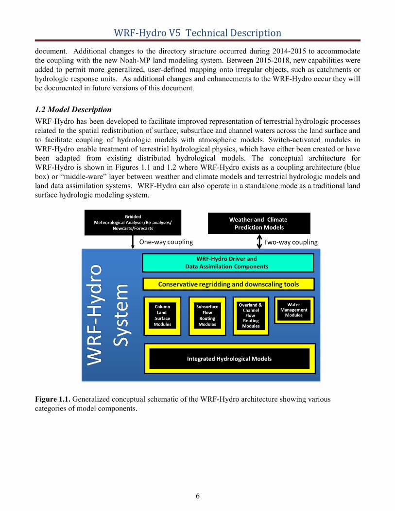
1.2 Model Description WRF-Hydro has been developed to facilitate improved representation of terrestrial hydrologic processes related to the spatial redistribution of surface, subsurface and channel waters across the land surface and to facilitate coupling of hydrologic models with atmospheric models. Switch-activated modules in WRF-Hydro enable treatment of terrestrial hydrological physics, which have either been created or have been adapted from existing distributed hydrological models. The conceptual architecture for WRF-Hydro is shown in Figures 1.1 and 1.2 where WRF-Hydro exists as a coupling architecture (blue box) or “middle-ware” layer between weather and climate models and terrestrial hydrologic models and land data assimilation systems. WRF-Hydro can also operate in a standalone mode as a traditional land surface hydrologic modeling system.
Figure 1.1. Generalized conceptual schematic of the WRF-Hydro architecture showing various categories of model components.
6
WRF-Hydro V5 Technical Description
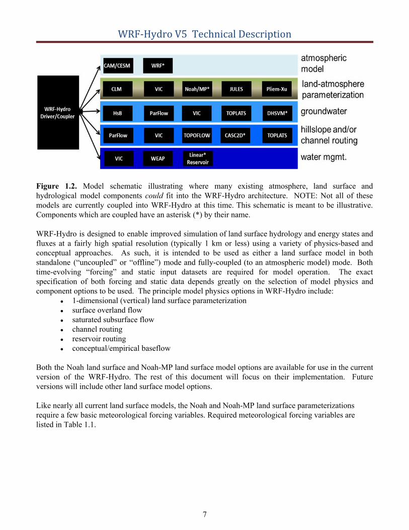
Figure 1.2. Model schematic illustrating where many existing atmosphere, land surface and hydrological model components could fit into the WRF-Hydro architecture. NOTE: Not all of these models are currently coupled into WRF-Hydro at this time. This schematic is meant to be illustrative. Components which are coupled have an asterisk (*) by their name.
WRF-Hydro is designed to enable improved simulation of land surface hydrology and energy states and fluxes at a fairly high spatial resolution (typically 1 km or less) using a variety of physics-based and conceptual approaches. As such, it is intended to be used as either a land surface model in both standalone (“uncoupled” or “offline”) mode and fully-coupled (to an atmospheric model) mode. Both time-evolving “forcing” and static input datasets are required for model operation. The exact specification of both forcing and static data depends greatly on the selection of model physics and component options to be used. The principle model physics options in WRF-Hydro include:
● 1-dimensional (vertical) land surface parameterization● surface overland flow● saturated subsurface flow● channel routing● reservoir routing● conceptual/empirical baseflow
Both the Noah land surface and Noah-MP land surface model options are available for use in the current version of the WRF-Hydro. The rest of this document will focus on their implementation. Future versions will include other land surface model options.
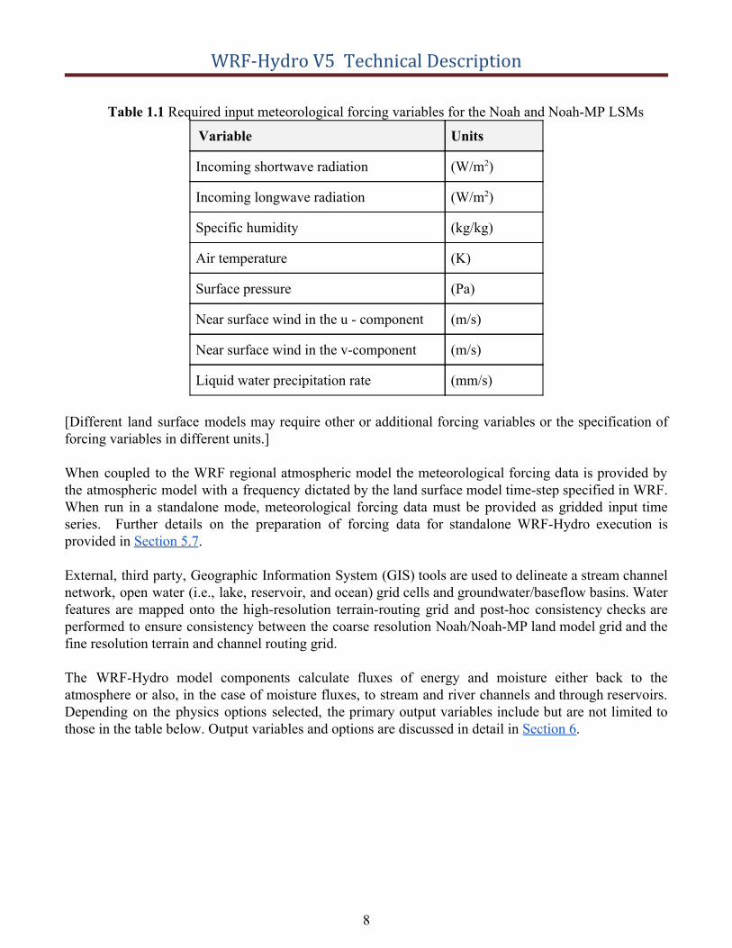
Like nearly all current land surface models, the Noah and Noah-MP land surface parameterizations require a few basic meteorological forcing variables. Required meteorological forcing variables are listed in Table 1.1.
7
WRF-Hydro V5 Technical Description
Table 1.1 Required input meteorological forcing variables for the Noah and Noah-MP LSMs
Variable Units
Incoming shortwave radiation (W/m2)
Incoming longwave radiation (W/m2)
Specific humidity (kg/kg)
Air temperature (K)
Surface pressure (Pa)
Near surface wind in the u - component (m/s)
Near surface wind in the v-component (m/s)
Liquid water precipitation rate (mm/s)
[Different land surface models may require other or additional forcing variables or the specification of forcing variables in different units.]
When coupled to the WRF regional atmospheric model the meteorological forcing data is provided by the atmospheric model with a frequency dictated by the land surface model time-step specified in WRF. When run in a standalone mode, meteorological forcing data must be provided as gridded input time series. Further details on the preparation of forcing data for standalone WRF-Hydro execution is provided in Section 5.7.
External, third party, Geographic Information System (GIS) tools are used to delineate a stream channel network, open water (i.e., lake, reservoir, and ocean) grid cells and groundwater/baseflow basins. Water features are mapped onto the high-resolution terrain-routing grid and post-hoc consistency checks are performed to ensure consistency between the coarse resolution Noah/Noah-MP land model grid and the fine resolution terrain and channel routing grid.
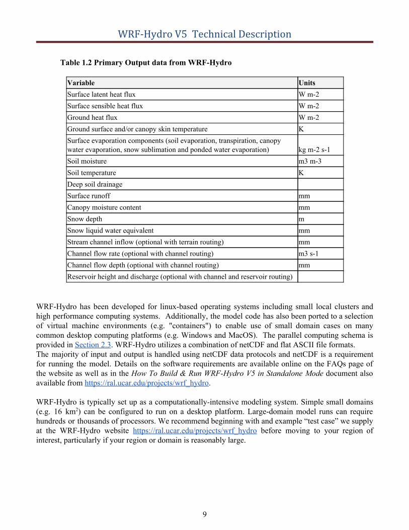
The WRF-Hydro model components calculate fluxes of energy and moisture either back to the atmosphere or also, in the case of moisture fluxes, to stream and river channels and through reservoirs. Depending on the physics options selected, the primary output variables include but are not limited to those in the table below. Output variables and options are discussed in detail in Section 6.
8
WRF-Hydro V5 Technical Description
Table 1.2 Primary Output data from WRF-Hydro
Variable Units Surface latent heat flux W m-2 Surface sensible heat flux W m-2 Ground heat flux W m-2 Ground surface and/or canopy skin temperature K Surface evaporation components (soil evaporation, transpiration, canopy water evaporation, snow sublimation and ponded water evaporation) kg m-2 s-1 Soil moisture m3 m-3 Soil temperature K Deep soil drainage Surface runoff mm Canopy moisture content mm Snow depth m Snow liquid water equivalent mm Stream channel inflow (optional with terrain routing) mm Channel flow rate (optional with channel routing) m3 s-1 Channel flow depth (optional with channel routing) mm Reservoir height and discharge (optional with channel and reservoir routing)
WRF-Hydro has been developed for linux-based operating systems including small local clusters and high performance computing systems. Additionally, the model code has also been ported to a selection of virtual machine environments (e.g. "containers") to enable use of small domain cases on many common desktop computing platforms (e.g. Windows and MacOS). The parallel computing schema is provided in Section 2.3. WRF-Hydro utilizes a combination of netCDF and flat ASCII file formats. The majority of input and output is handled using netCDF data protocols and netCDF is a requirement for running the model. Details on the software requirements are available online on the FAQs page of the website as well as in the How To Build & Run WRF-Hydro V5 in Standalone Mode document also available from https://ral.ucar.edu/projects/wrf_hydro .
WRF-Hydro is typically set up as a computationally-intensive modeling system. Simple small domains (e.g. 16 km2) can be configured to run on a desktop platform. Large-domain model runs can require hundreds or thousands of processors. We recommend beginning with and example “test case” we supply at the WRF-Hydro website https://ral.ucar.edu/projects/wrf_hydro before moving to your region of interest, particularly if your region or domain is reasonably large.
9
WRF-Hydro V5 Technical Description
2. Model Code and Configuration DescriptionThis chapter presents the technical description of the WRF-Hydro model code. The chapter is divided into the following sections:
2.1. Brief code overview 2.2. Driver level description 2.3. Parallelization strategy 2.4. Directory structures 2.5. Model sequence of operations 2.6. WRF-Hydro compile-time options 2.7. WRF-Hydro run-time options
2.1 Brief code overview WRF-Hydro is written in a modularized, FORTRAN90 coding structure whose routing physics modules are switch activated through a model namelist file hydro.namelist . The code has been parallelized for execution on high-performance, parallel computing architectures including LINUX operating system commodity clusters and multi-processor desktops as well as multiple supercomputers. More detailed model requirements depend on the choice of model driver, described in the next section.
2.2 Driver level description WRF-Hydro is essentially a group of modules and functions which handle the communication of information between atmosphere components (such as WRF, CESM or prescribed meteorological analyses) and sets of land surface hydrology components. From a coding perspective the WRF-hydro system can be called from an existing architecture such as the WRF model, the CESM, NASA LIS, etc. or can run in a standalone mode with its own driver which has adapted part of the NCAR High Resolution Land Data Assimilation System (HRLDAS). Each new coupling effort requires some basic modifications to a general set of functions to manage the coupling. In WRF-Hydro, each new system that WRF-Hydro is coupled into gets assigned to a directory indicating the name of the coupling component WRF-Hydro is coupled to. For instance, the code which handles the coupling to the WRF model is contained in the WRF_cpl/ directory in the WRF-Hydro system. Similarly, the code which handles the coupling to the offline Noah land surface modeling system is contained within the Noah_cpl / directory and so on. Description of each directory is provided in Section 2.4.
The coupling structure is illustrated here, briefly, in terms of the coupling of WRF-Hydro into the WRF model. A similar approach is used for coupling the WRF-Hydro extension package into other modeling systems or for coupling other modeling systems into WRF-Hydro.
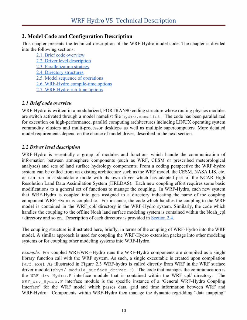
Example: For coupled WRF/WRF-Hydro runs the WRF-Hydro components are compiled as a single library function call with the WRF system. As such, a single executable is created upon compilation (wrf.exe ). As illustrated in Figure 2.3 WRF-hydro is called directly from WRF in the WRF surface driver module (phys/ module_surface_driver.F ). The code that manages the communication is the WRF_drv_Hydro.F interface module that is contained within the WRF_cpl/ directory. The WRF_drv_Hydro.F interface module is the specific instance of a ‘General WRF-Hydro Coupling Interface’ for the WRF model which passes data, grid and time information between WRF and WRF-Hydro. Components within WRF-Hydro then manage the dynamic regridding “data mapping”
10
WRF-Hydro V5 Technical Description
and sub-component routing functions (e.g. surface, subsurface and/or channel routing) within WRF-Hydro (see Fig. 1.1 for an illustration of components contained within WRF-Hydro). Upon completion of the user-specified routing functions, WRF-Hydro will remap the data back to the WRF model grid and then pass the necessary variables back to the WRF model through the WRF_drv_Hydro.F interface module. Therefore, the key component of the WRF-Hydro system is the proper construction of the WRF_cpl_Hydro interface module (or more generally ‘XXX_cpl_Hydro’). Users wishing to couple new modules to WRF-Hydro will need to create a unique “General WRF-Hydro Coupling Interface” for their components. Some additional examples of this interface module are available upon request for users to build new coupling components. This simple coupling interface is similar in structure to other general model coupling interfaces such as those within the Earth System Modeling Framework (ESMF) or the Community Surface Dynamics Modeling System (CSDMS).
Figure 2.1 Schematic illustrating the coupling and calling structure of WRF-Hydro from the WRF Model.
The model code has been compiled using the PGI Fortran compiler, the Intel ‘ifort’ compiler and the public license GNU Fortran compiler ‘gfortran’ for use with Linux-based operating systems on desktops, clusters, and supercomputing systems.Because the WRF-Hydro modeling system relies on netCDF input and output file conventions, netCDF Fortran libraries must be installed and properly compiled on the system upon which WRF-Hydro is to be executed. Not doing so will result in numerous error messages such as ‘…undefined reference to netCDF library … ’ or similar messages upon compilation. For further installation requirements see the FAQs page of the website as well as in the How To Build & Run WRF-Hydro V5 in Standalone Mode document also available from https://ral.ucar.edu/projects/wrf_hydro .
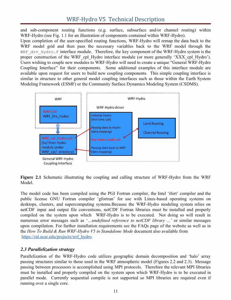
2.3 Parallelization strategy Parallelization of the WRF-Hydro code utilizes geographic domain decomposition and ‘halo’ array passing structures similar to those used in the WRF atmospheric model (Figures 2.2 and 2.3). Message passing between processors is accomplished using MPI protocols. Therefore the relevant MPI libraries must be installed and properly compiled on the system upon which WRF-Hydro is to be executed in parallel mode. Currently sequential compile is not supported so MPI libraries are required even if running over a single core.
11
WRF-Hydro V5 Technical Description
Figure 2.2 Schematic of parallel domain decomposition scheme in WRF-Hydro. Boundary or ‘halo’ arrays in which memory is shared between processors (P1 and P2) are shaded in purple.
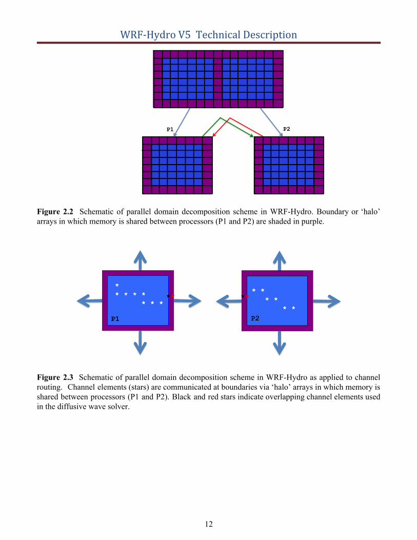
Figure 2.3 Schematic of parallel domain decomposition scheme in WRF-Hydro as applied to channel routing. Channel elements (stars) are communicated at boundaries via ‘halo’ arrays in which memory is shared between processors (P1 and P2). Black and red stars indicate overlapping channel elements used in the diffusive wave solver.
12
WRF-Hydro V5 Technical Description
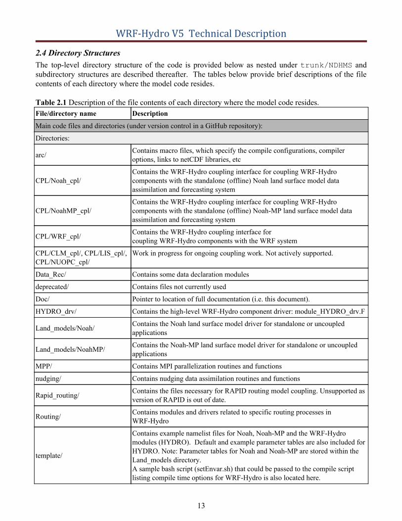
2.4 Directory Structures The top-level directory structure of the code is provided below as nested under trunk/NDHMS and subdirectory structures are described thereafter. The tables below provide brief descriptions of the file contents of each directory where the model code resides.
Table 2.1 Description of the file contents of each directory where the model code resides. File/directory name Description
Main code files and directories (under version control in a GitHub repository):
Directories:
arc/ Contains macro files, which specify the compile configurations, compiler options, links to netCDF libraries, etc
CPL/Noah_cpl/ Contains the WRF-Hydro coupling interface for coupling WRF-Hydro components with the standalone (offline) Noah land surface model data assimilation and forecasting system
CPL/NoahMP_cpl/ Contains the WRF-Hydro coupling interface for coupling WRF-Hydro components with the standalone (offline) Noah-MP land surface model data assimilation and forecasting system
CPL/WRF_cpl/ Contains the WRF-Hydro coupling interface for coupling WRF-Hydro components with the WRF system
CPL/CLM_cpl/, CPL/LIS_cpl/, CPL/NUOPC_cpl/
Work in progress for ongoing coupling work. Not actively supported.
Data_Rec/ Contains some data declaration modules
deprecated/ Contains files not currently used
Doc/ Pointer to location of full documentation (i.e. this document).
HYDRO_drv/ Contains the high-level WRF-Hydro component driver: module_HYDRO_drv.F
Land_models/Noah/ Contains the Noah land surface model driver for standalone or uncoupled applications
Land_models/NoahMP/ Contains the Noah-MP land surface model driver for standalone or uncoupled applications
MPP/ Contains MPI parallelization routines and functions
nudging/ Contains nudging data assimilation routines and functions
Rapid_routing/ Contains the files necessary for RAPID routing model coupling. Unsupported as version of RAPID is out of date.
Routing/ Contains modules and drivers related to specific routing processes in WRF-Hydro
template/
Contains example namelist files for Noah, Noah-MP and the WRF-Hydro modules (HYDRO). Default and example parameter tables are also included for HYDRO. Note: Parameter tables for Noah and Noah-MP are stored within the Land_models directory. A sample bash script (setEnvar.sh) that could be passed to the compile script listing compile time options for WRF-Hydro is also located here.
13
WRF-Hydro V5 Technical Description
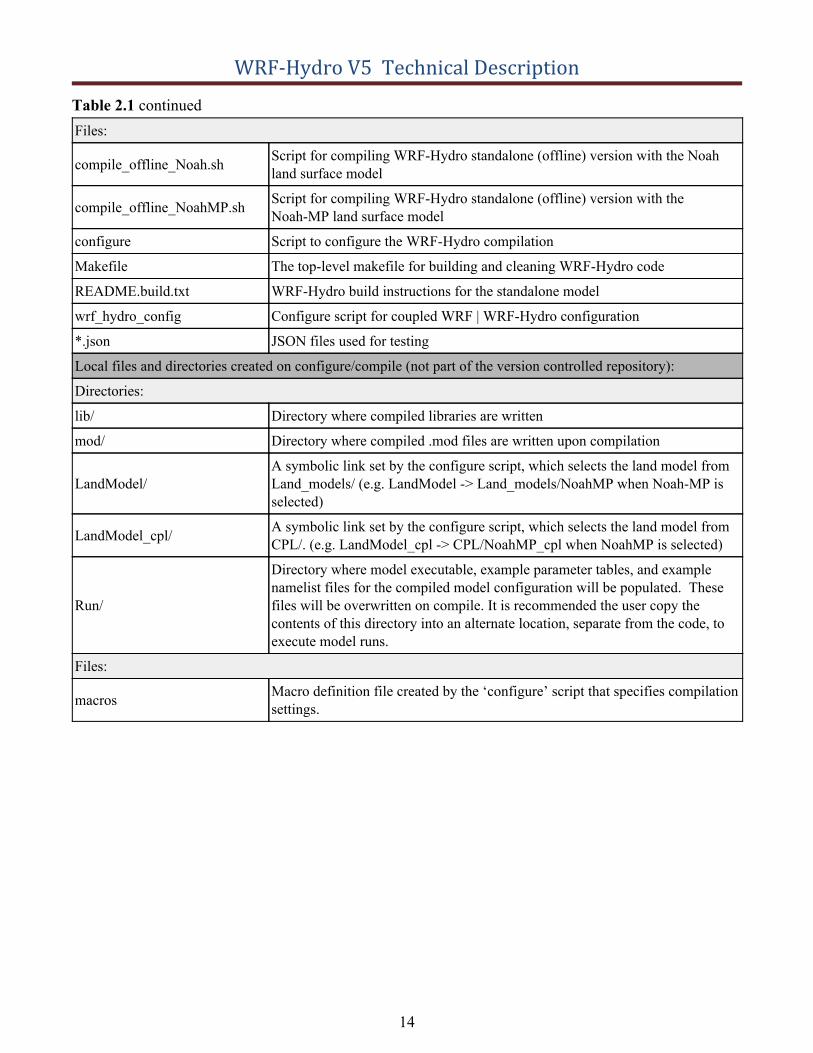
Table 2.1 continued Files:
compile_offline_Noah.sh Script for compiling WRF-Hydro standalone (offline) version with the Noah land surface model
compile_offline_NoahMP.sh Script for compiling WRF-Hydro standalone (offline) version with the Noah-MP land surface model
configure Script to configure the WRF-Hydro compilation
Makefile The top-level makefile for building and cleaning WRF-Hydro code
README.build.txt WRF-Hydro build instructions for the standalone model
wrf_hydro_config Configure script for coupled WRF | WRF-Hydro configuration
*.json JSON files used for testing
Local files and directories created on configure/compile (not part of the version controlled repository):
Directories:
lib/ Directory where compiled libraries are written
mod/ Directory where compiled .mod files are written upon compilation
LandModel/ A symbolic link set by the configure script, which selects the land model from Land_models/ (e.g. LandModel -> Land_models/NoahMP when Noah-MP is selected)
LandModel_cpl/ A symbolic link set by the configure script, which selects the land model from CPL/. (e.g. LandModel_cpl -> CPL/NoahMP_cpl when NoahMP is selected)
Run/
Directory where model executable, example parameter tables, and example namelist files for the compiled model configuration will be populated. These files will be overwritten on compile. It is recommended the user copy the contents of this directory into an alternate location, separate from the code, to execute model runs.
Files:
macros Macro definition file created by the ‘configure’ script that specifies compilation settings.
14
WRF-Hydro V5 Technical Description
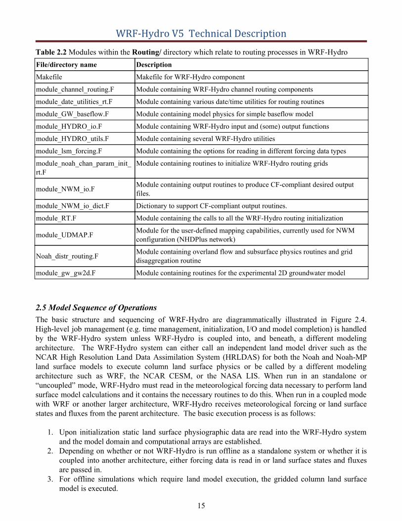
Table 2.2 Modules within the Routing/ directory which relate to routing processes in WRF-Hydro File/directory name Description
Makefile Makefile for WRF-Hydro component
module_channel_routing.F Module containing WRF-Hydro channel routing components
module_date_utilities_rt.F Module containing various date/time utilities for routing routines
module_GW_baseflow.F Module containing model physics for simple baseflow model
module_HYDRO_io.F Module containing WRF-Hydro input and (some) output functions
module_HYDRO_utils.F Module containing several WRF-Hydro utilities
module_lsm_forcing.F Module containing the options for reading in different forcing data types
module_noah_chan_param_init_rt.F
Module containing routines to initialize WRF-Hydro routing grids
module_NWM_io.F Module containing output routines to produce CF-compliant desired output files.
module_NWM_io_dict.F Dictionary to support CF-compliant output routines.
module_RT.F Module containing the calls to all the WRF-Hydro routing initialization
module_UDMAP.F Module for the user-defined mapping capabilities, currently used for NWM configuration (NHDPlus network)
Noah_distr_routing.F Module containing overland flow and subsurface physics routines and grid disaggregation routine
module_gw_gw2d.F Module containing routines for the experimental 2D groundwater model
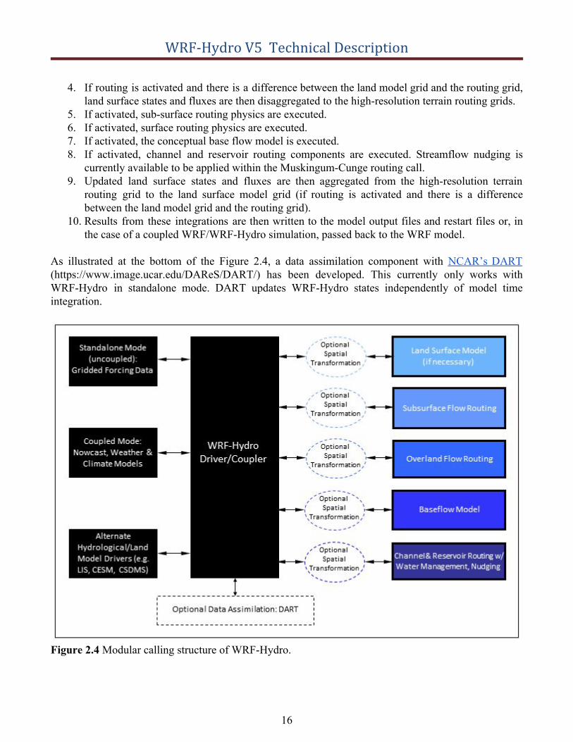
2.5 Model Sequence of Operations The basic structure and sequencing of WRF-Hydro are diagrammatically illustrated in Figure 2.4. High-level job management (e.g. time management, initialization, I/O and model completion) is handled by the WRF-Hydro system unless WRF-Hydro is coupled into, and beneath, a different modeling architecture. The WRF-Hydro system can either call an independent land model driver such as the NCAR High Resolution Land Data Assimilation System (HRLDAS) for both the Noah and Noah-MP land surface models to execute column land surface physics or be called by a different modeling architecture such as WRF, the NCAR CESM, or the NASA LIS. When run in an standalone or “uncoupled” mode, WRF-Hydro must read in the meteorological forcing data necessary to perform land surface model calculations and it contains the necessary routines to do this. When run in a coupled mode with WRF or another larger architecture, WRF-Hydro receives meteorological forcing or land surface states and fluxes from the parent architecture. The basic execution process is as follows:
1. Upon initialization static land surface physiographic data are read into the WRF-Hydro system and the model domain and computational arrays are established.
2. Depending on whether or not WRF-Hydro is run offline as a standalone system or whether it is coupled into another architecture, either forcing data is read in or land surface states and fluxes are passed in.
3. For offline simulations which require land model execution, the gridded column land surface model is executed.
15
WRF-Hydro V5 Technical Description
4. If routing is activated and there is a difference between the land model grid and the routing grid, land surface states and fluxes are then disaggregated to the high-resolution terrain routing grids.
5. If activated, sub-surface routing physics are executed.6. If activated, surface routing physics are executed.7. If activated, the conceptual base flow model is executed.8. If activated, channel and reservoir routing components are executed. Streamflow nudging is
currently available to be applied within the Muskingum-Cunge routing call.9. Updated land surface states and fluxes are then aggregated from the high-resolution terrain
routing grid to the land surface model grid (if routing is activated and there is a difference between the land model grid and the routing grid).
10. Results from these integrations are then written to the model output files and restart files or, in the case of a coupled WRF/WRF-Hydro simulation, passed back to the WRF model.
As illustrated at the bottom of the Figure 2.4, a data assimilation component with NCAR’s DART (https://www.image.ucar.edu/DAReS/DART/) has been developed. This currently only works with WRF-Hydro in standalone mode. DART updates WRF-Hydro states independently of model time integration.
Figure 2.4 Modular calling structure of WRF-Hydro.
16
WRF-Hydro V5 Technical Description
2.6 WRF-Hydro compile-time options Compile time options are choices about the model structure which are determined when the model is compiled. Compile time choices select a WRF-Hydro instance from some of the options illustrated in Figure 2.4. Compile time options fall into two categories: 1) what is the selected model driver, and 2) what are the compile options for the that choice of driver. In this guide we limit the description of model drivers to WRF, Noah, and Noah-MP. Configuring, compiling, and running WRF-Hydro in standalone mode is described in detail in the How To Build & Run WRF-Hydro V5 in Standalone Mode document available from https://ral.ucar.edu/projects/wrf_hydro.
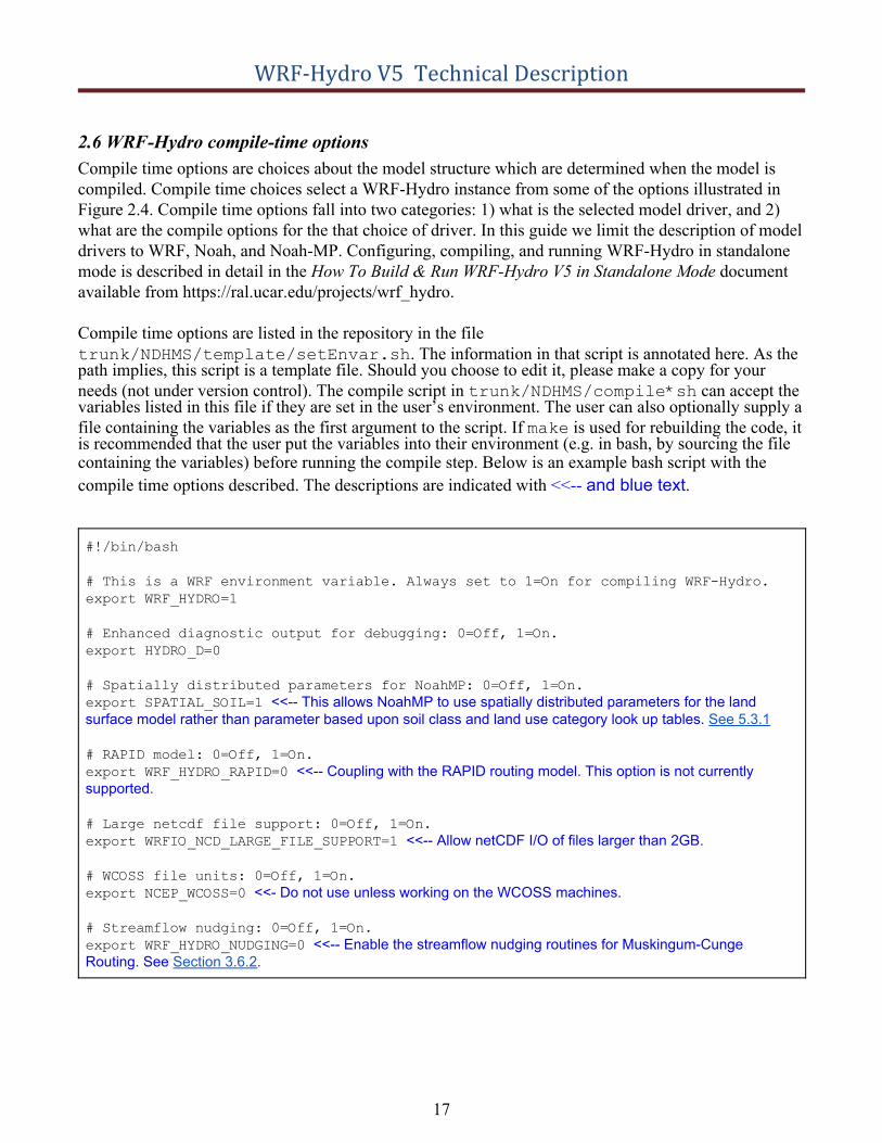
Compile time options are listed in the repository in the file trunk/NDHMS/template/setEnvar.sh . The information in that script is annotated here. As thepath implies, this script is a template file. Should you choose to edit it, please make a copy for your needs (not under version control). The compile script in trunk/NDHMS/compile*sh can accept thevariables listed in this file if they are set in the user’s environment. The user can also optionally supply a file containing the variables as the first argument to the script. If make is used for rebuilding the code, itis recommended that the user put the variables into their environment (e.g. in bash, by sourcing the file containing the variables) before running the compile step. Below is an example bash script with the compile time options described. The descriptions are indicated with <<-- and blue text .
#!/bin/bash
# This is a WRF environment variable. Always set to 1=On for compiling WRF-Hydro.
export WRF_HYDRO=1
# Enhanced diagnostic output for debugging: 0=Off, 1=On.
export HYDRO_D=0
# Spatially distributed parameters for NoahMP: 0=Off, 1=On.
export SPATIAL_SOIL=1 <<-- This allows NoahMP to use spatially distributed parameters for the landsurface model rather than parameter based upon soil class and land use category look up tables. See 5.3.1
# RAPID model: 0=Off, 1=On.
export WRF_HYDRO_RAPID=0 <<-- Coupling with the RAPID routing model. This option is not currentlysupported.
# Large netcdf file support: 0=Off, 1=On.
export WRFIO_NCD_LARGE_FILE_SUPPORT=1 <<-- Allow netCDF I/O of files larger than 2GB.
# WCOSS file units: 0=Off, 1=On.
export NCEP_WCOSS=0 <<- Do not use unless working on the WCOSS machines.
# Streamflow nudging: 0=Off, 1=On.
export WRF_HYDRO_NUDGING=0 <<-- Enable the streamflow nudging routines for Muskingum-CungeRouting. See Section 3.6.2.
17
WRF-Hydro V5 Technical Description
2.7 WRF-Hydro run time options There are two namelist files that users must edit in order to successfully execute the WRF-Hydro system in a standalone mode or “uncoupled” to WRF. One of these namelist files is the hydro.namelist file and in it are the various settings for operating all of the routing components of the WRF-Hydro system. The hydro.namelist file is internally commented so that it should be clear as to what isneeded for each setting. A full annotated example of the hydro.namelist file is provided inAppendix A5.
The second namelist is the namelist which specifies the land surface model options to be used. This namelist can change depending on which land model is to be used in conjunction with the WRF-Hydro routing components. For example, a user would use one namelist when running the Noah land surface model coupled to WRF-Hydro but that user would need to use a different namelist file when running the CLM model, the Noah-MP model or NASA LIS model coupled to WRF-Hydro. The reason for this is WRF-Hydro is intended to be ‘minimally-invasive’ to other land surface models or land model driver structures and not require significant changes to those systems. This minimal invasiveness facilitates easier coupling with new systems and helps facilitate easy supportability and version control with those systems. When the standalone WRF-Hydro model is compiled the appropriate namelist.hrldas template file is copied over to the Run directory based upon the specified land surface model.
In WRF-Hydro v5.0, the Noah and Noah-MP land surface models are the main land surface model options when WRF-Hydro is run in standalone mode. Both Noah and Noah-MP use a namelist file called namelist.hrldas , which, as noted above, will contain different settings for the two differentland surface models. For a run where WRF-Hydro is coupled to the WRF model, the WRF model input file namelist.input becomes the second namelist file. Full annotated examplenamelist.hrldas files for Noah and Noah-MP are provided in Appendix A3 and Appendix A4.
18
WRF-Hydro V5 Technical Description
3. Model Physics DescriptionThis chapter describes the physics behind each of the modules in Version 5.0 of WRF-Hydro and the associated namelist options which are specified at “run time”. The chapter is divided into the following sections:
3.1. Physics Overview 3.2. Land Model Description: The community Noah and Noah-MP land surface models 3.3. Spatial Transformations
3.3.1 Subgrid Disaggregation-aggregation 3.3.2 User-Defined Mapping 3.3.3 Data Remapping for Hydrological Applications
3.4 Subsurface Routing 3.5 Surface Overland Flow Routing 3.6 Channel and Lake Routing
3.6.1. Gridded Routing using Diffusive Wave 3.6.2. Linked Routing using Muskingum and Muskingum-Cunge
3.7 Lake and Reservoir routing description 3.8 Conceptual base flow model description
3.1 Physics Overview
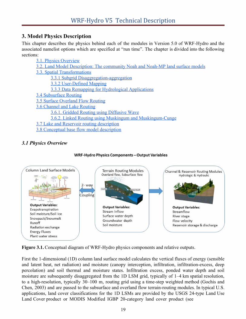
Figure 3.1. Conceptual diagram of WRF-Hydro physics components and relative outputs.
First the 1-dimensional (1D) column land surface model calculates the vertical fluxes of energy (sensible and latent heat, net radiation) and moisture (canopy interception, infiltration, infiltration-excess, deep percolation) and soil thermal and moisture states. Infiltration excess, ponded water depth and soil moisture are subsequently disaggregated from the 1D LSM grid, typically of 1–4 km spatial resolution, to a high-resolution, typically 30–100 m, routing grid using a time-step weighted method (Gochis and Chen, 2003) and are passed to the subsurface and overland flow terrain-routing modules. In typical U.S. applications, land cover classifications for the 1D LSMs are provided by the USGS 24-type Land Use Land Cover product or MODIS Modified IGBP 20-category land cover product (see
19
WRF-Hydro V5 Technical Description
WRF/WPS documentation); soil classifications are provided by the 1-km STATSGO database (Miller and White, 1998); and soil hydraulic parameters that are mapped to the STATSGO soil classes are specified by the soil analysis of Cosby et al. (1984). Other land cover and soil type classification datasets can be used with WRF-Hydro but users are responsible for mapping those categories back to the same categories as used in the USGS or MODIS land cover and STATSGO soil type datasets. The WRF model pre-processing system (WPS) also provides a fairly comprehensive database of land surface data that can be used to set up the Noah and Noah-MP land surface models. It is possible to use other land cover and soils datasets.
Then subsurface lateral flow in WRF-Hydro is calculated prior to the routing of overland flow to allow exfiltration from fully saturated grid cells to be added to the infiltration excess calculated from the LSM. The current existing method used to calculate the lateral flow of saturated soil moisture is that of Wigmosta et al. (1994) and Wigmosta and Lettenmaier (1999), implemented in the Distributed Hydrology Soil Vegetation Model (DHSVM). It calculates a quasi-3D flow, which includes the effects of topography, saturated soil depth, and depth-varying saturated hydraulic conductivity values. Hydraulic gradients are approximated as the slope of the water table between adjacent grid cells in either the steepest descent or in both x- and y-directions. The flux of water from one cell to its down-gradient neighbor on each time-step is approximated as a steady-state solution.
Next, WRF-Hydro specifies the water table depth according the depth of the top of the saturated soil layer that is nearest to the surface. Typically, a minimum of four soil layers are used in a 2-meter soil column used in WRF-Hydro but this is not a strict requirement. Additional discretization permits improved resolution of a time-varying water table height and users may vary the number and thickness of soil layers in the model namelist described in the Appendices A3, A4, and A5.
Then overland flow is defined. The fully unsteady, spatially explicit, diffusive wave formulation of Julien et al. (1995-CASC2D) with later modification by Ogden (1997) is the current option for representing overland flow, which is calculated when the depth of water on a model grid cell exceeds a specified retention depth. The diffusive wave equation accounts for backwater effects and allows for flow on adverse slopes (Ogden, 1997). As in Julien et al. (1995), the continuity equation for an overland flood wave is combined with the diffusive wave formulation of the momentum equation. Manning’s equation is used as the resistance formulation for momentum and requires specification of an overland flow roughness parameter. Values of the overland flow roughness coefficient used in WRF-Hydro were obtained from Vieux (2001) and were mapped to the existing land cover classifications provided by the USGS 24-type land-cover product of Loveland et al. (1995) and the MODIS 20-type land cover product, which are the same land cover classification datasets used in the 1D Noah/Noah-MP LSMs.
Additional modules have also been implemented to represent stream channel flow processes, lakes and reservoirs, and stream baseflow. In WRF-Hydro v5.0 inflow into the stream network and lake and reservoir objects is a one-way process. Overland flow reaching grid cells identified as ‘channel’ grid cells pass a portion of the surface water in excess of the local ponded water retention depth to the channel model. This current formulation implies that stream and lake inflow from the land surface is always positive to the stream or lake element. There currently are no channel or lake loss functions where water can move from channels or lakes back to the landscape. Channel flow in WRF-Hydro is represented by one of a few different user-selected methodologies described below. Water passing into and through lakes and reservoirs is routed using a simple level pool routing scheme. Baseflow to the stream network is represented using a conceptual catchment storage-discharge bucket model formulation (discussed below) which obtains “drainage” flow from the spatially-distributed landscape. Discharge
20
WRF-Hydro V5 Technical Description
from buckets is input directly into the stream using an empirically-derived storage-discharge relationship. If overland flow is active, the only water flowing into the buckets comes from soil drainage. This is because the overland flow scheme will pass water directly to the channel model. If overland flow is switched off and channel routing is still active, then surface infiltration excess water from the land model is collected over the pre-defined catchment and passed into the bucket as well. Each of these process options are enabled through the specification of options in the model namelist file.
3.2 Land model description: The community Noah and Noah-MP land surface models [NOTE: As of this writing, only the Noah and Noah-MP land surface models are supported within WRF-Hydro. Additional land surface models such as CLM or land model driver frameworks, such as the NASA Land Information System (LIS) have been coupled with WRF-Hydro but those efforts are in various phases of development and are not yet formally supported as part of the main code repository. ]
The Noah land surface model is a community, 1-dimensional land surface model that simulates soil moisture (both liquid and frozen), soil temperature, skin temperature, snowpack depth, snowpack water equivalent, canopy water content and the energy flux and water flux terms at the Earth’s surface (Mitchell et al., 2002; Ek et al., 2003). The model has a long heritage, with legacy versions extensively tested and validated, most notably within the Project for Intercomparison of Land surface Parameterizations (PILPS), the Global Soil Wetness Project (Dirmeyer et al. 1999), and the Distributed Model Intercomparison Project (Smith, 2002). Mahrt and Pan (1984) and Pan and Mahrt (1987) developed the earliest predecessor to Noah at Oregon State University (OSU) during the mid-1980’s. The original OSU model calculated sensible and latent heat flux using a two-layer soil model and a simplified plant canopy model. Recent development and implementation of the current version of Noah has been sustained through the community participation of various agency modeling groups and the university community (e.g. Chen et al., 2005). Ek et al. (2003) detail the numerous changes that have evolved since its inception including, a four layer soil representation (with soil layer thicknesses of 0.1, 0.3, 0.6 and 1.0 m), modifications to the canopy conductance formulation (Chen et al., 1996), bare soil evaporation and vegetation phenology (Betts et al., 1997), surface runoff and infiltration (Schaake et al., 1996), thermal roughness length treatment in the surface layer exchange coefficients (Chen et al., 1997a) and frozen soil processes (Koren et al., 1999). More recently refinements to the snow-surface energy budget calculation (Ek et al., 2003) and seasonal variability of the surface emissivity (Tewari et al., 2005) have been implemented.
The Noah land surface model has been tested extensively in both offline (e.g., Chen et al., 1996, 1997; Chen and Mitchell, 1999; Wood et al., 1998; Bowling et al., 2003) and coupled (e.g. Chen et el., 1997, Chen and Dudhia, 2001, Yucel et al., 1998; Angevine and Mitchell, 2001; and Marshall et al., 2002) modes. The most recent version of Noah is currently one of the operational LSP’s participating in the interagency NASA-NCEP real-time Land Data Assimilation System (LDAS, 2003, Mitchell et al., 2004 for details). Gridded versions of the Noah model are currently coupled to real-time weather forecasting models such as the National Center for Environmental Prediction (NCEP) North American Model (NAM), and the community WRF model. Users are referred to Ek et al. (2003) and earlier works for more detailed descriptions of the 1-dimensional land surface model physics of the Noah LSM.
Support for the Noah Land Surface Model within WRF-Hydro is currently frozen at Noah version 3.6. Since the Noah LSM is not under active development by the community, WRF-Hydro is continuing to support Noah in deprecated mode only. Some new model features, such as the improved output routines,
21
WRF-Hydro V5 Technical Description
have not been setup to be backward compatible with Noah. Noah users should follow the guidelines in Appendix A2 for adapting the WRF-Hydro workflow to work with Noah.
Noah-MP is a land surface model (LSM) using multiple options for key land-atmosphere interaction processes (Niu et al., 2011). Noah-MP was developed to improve upon some of the limitations of the Noah LSM (Koren et al., 1999; Ek et al., 2003). Specifically, Noah-MP contains a separate vegetation canopy defined by a canopy top and bottom, crown radius, and leaves with prescribed dimensions, orientation, density, and radiometric properties. The canopy employs a two-stream radiation transfer approach along with shading effects necessary to achieve proper surface energy and water transfer processes including under-canopy snow processes (Dickinson, 1983; Niu and Yang, 2004). Noah-MP contains a multi-layer snow pack with liquid water storage and melt/refreeze capability and a snow-interception model describing loading/unloading, melt/refreeze capability, and sublimation of canopy-intercepted snow (Yang and Niu 2003; Niu and Yang 2004). Multiple options are available for surface water infiltration and runoff and groundwater transfer and storage including water table depth to an unconfined aquifer (Niu et al., 2007).
The Noah-MP land surface model can be executed by prescribing both the horizontal and vertical density of vegetation using either ground- or satellite-based observations. Another available option is for prognostic vegetation growth that combines a Ball-Berry photosynthesis-based stomatal resistance (Ball et al., 1987) with a dynamic vegetation model (Dickinson et al. 1998) that allocates carbon to various parts of vegetation (leaf, stem, wood and root) and soil carbon pools (fast and slow). The model is capable of distinguishing between C3 and C4 photosynthesis pathways and defines vegetation-specific parameters for plant photosynthesis and respiration.
3.3 Spatial Transformations The WRF-Hydro system has the ability to execute a number of physical process executions (e.g. column physics, routing processes, reservoir fluxes) on different spatial frameworks (e.g. regular grids, catchments, river channel vectors, reservoir polygons, etc). This means that spatial transformations between differing spatial elements has become a critical part of the overall modeling process. Starting in v5.0 of WRF-Hydro, increased support has been developed to aid in the mapping between differing spatial frameworks. Section 3.3.1 describes the spatial transformation process which relies on regular, rectilinear grid-to-grid mapping using a simplified integer linear multiple aggregation/disaggregation scheme. This basic scheme has been utilized in WRF-Hydro since its creation as it was described in Gochis and Chen, 2003. The following section 3.3.2 describes new spatial transformation methods that have been developed and are currently supported in v5.0 and, more specifically, in the NOAA National Water Model (NWM). Those user-defined transformations rely on the pre-processing development and specification of interpolation or mapping weights which must be read into the model. As development continues future versions will provide more options and flexibility for spatial transformations using similar user-defined methodologies.
22
WRF-Hydro V5 Technical Description
3.3.1 Subgrid disaggregation-aggregation This section details the implementation of a subgrid aggregation/disaggregation scheme in WRF-Hydro. The disaggregation-aggregation routines are activated when routing of either overland flow or subsurface flow is active and the specified routing grid increment is different from that of the land surface model grid. Routing in WRF-Hydro is “switch-activated” through the declaration of parameter options in the primary model namelist file hydro.namelist which are described in Appendix A5. In WRF-Hydro subgrid aggregation/disaggregation is used to represent overland and subsurface flow processes on grid scales much finer than the native land surface model grid. Hence, only routing is represented within a subgrid framework. It is possible to run both the land surface model and the routing model components on the same grid. This effectively means that the aggregation factor between the grids has a value of 1.0. This following section describes the aggregation/disaggregation methodology in the context of a “subgrid” routing implementation.
In WRF-Hydro the routing portions of the code have been structured so that it is simple to perform both surface and subsurface routing calculations on grid cells that potentially differ from the native land surface model grid sizes provided that each land surface model grid cell is divided into integer portions for routing. Hence routing calculations can be performed on comparatively high-resolution land surfaces (e.g., a 25-m digital elevation model) while the native land surface model can be run at much larger (e.g., 1 km) grid sizes. (In this example, the integer multiple of disaggregation in this example would be equal to 40.) This capability adds considerable flexibility in the implementation of WRF-Hydro. However, it is well recognized that surface hydrological responses exhibit strongly scale-dependent behavior such that simulations at different scales, run with the same model forcing, may yield quite different results.
The aggregation/disaggregation routines are currently activated by specifying either the overland flow or subsurface flow routing options in the model namelist file and prescribing terrain grid domain file dimensions (IXRT,JXRT) which differ from the land surface model domain file dimensions (IX,JX). Additionally, the model sub-grid size (DXRT), the routing time-step (DTRT), and the integer divisor (AGGFACTRT), which determines how the aggregation/disaggregation routines will divide up a native model grid square, all need to be specified in the model hydro.namelist file.
If IXRT=IX, JXRT=JX and AGGFACTRT=1 the aggregation/disaggregation schemes will be activated but will not yield any effective changes in the model resolution between the land surface model grid and the terrain routing grid. Specifying different values for IXRT, JXRT and AGGFACTRT≠1 will yield effective changes in model resolution between the land model and terrain routing grids. As described in the Surface Overland Flow Routing section 3.5, DXRT and DTRT must always be specified in accordance with the routing grid even if they are the same as the native land surface model grid.
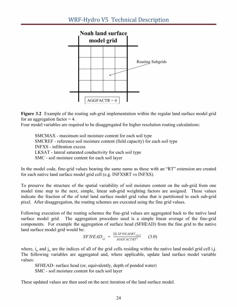
The disaggregation/aggregation routines are implemented in WRF-Hydro as two separate spatial loops that are executed after the main land surface model loop. The disaggregation loop is run prior to routing of saturated subsurface and surface water. The main purpose of the disaggregation loop is to divide up specific hydrologic state variables from the land surface model grid square into integer portions as specified by AGGFACTRT. An example disaggregation (where AGGFACTRT=4) is given in Figure 3.2.
23
WRF-Hydro V5 Technical Description
Figure 3.2 Example of the routing sub-grid implementation within the regular land surface model grid for an aggregation factor = 4. Four model variables are required to be disaggregated for higher resolution routing calculations:
SMCMAX - maximum soil moisture content for each soil type SMCREF - reference soil moisture content (field capacity) for each soil type
INFXS - infiltration excess LKSAT - lateral saturated conductivity for each soil type SMC - soil moisture content for each soil layer
In the model code, fine-grid values bearing the same name as these with an “RT” extension are created for each native land surface model grid cell (e.g. INFXSRT vs INFXS).
To preserve the structure of the spatial variability of soil moisture content on the sub-grid from one model time step to the next, simple, linear sub-grid weighting factors are assigned. These values indicate the fraction of the of total land surface model grid value that is partitioned to each sub-grid pixel. After disaggregation, the routing schemes are executed using the fine grid values.
Following execution of the routing schemes the fine-grid values are aggregated back to the native land surface model grid. The aggregation procedure used is a simple linear average of the fine-grid components. For example the aggregation of surface head (SFHEAD) from the fine grid to the native land surface model grid would be:
(3.0) SF HEADi,j = AGGF ACT RT 2
ΣΣ SF HEADRT irt,jrt
where, irt and jrt are the indices of all of the grid cells residing within the native land model grid cell i,j. The following variables are aggregated and, where applicable, update land surface model variable values:
SFHEAD- surface head (or, equivalently, depth of ponded water) SMC - soil moisture content for each soil layer
These updated values are then used on the next iteration of the land surface model.
24
WRF-Hydro V5 Technical Description
3.3.2 User-Defined Mapping The emergence of hydrologic models, like WRF-Hydro, that are capable of running on gridded as well as vector-based processing units requires generic tools for processing input and output data as well as methods for transferring data between models. Such a spatial transformation is currently utilized when mapping between model grids and catchments in the WRF-Hydro/National Water Model (NWM) system. In the NWM, selected model fluxes are mapped from WRF-Hydro model grids onto the NHDPlus catchment polygon and river vector network framework. The GIS pre-processing framework described here allows for fairly generalized geometric relationships between features to be characterized and for parameters to be summarized for any discrete unit of geography.
3.3.3 Data Remapping for Hydrological Applications
A common task in hydrologic modeling is to regrid or aggregate data from one unit of analysis to another. Frequently, atmospheric model data variables such as temperature and precipitation may be produced on a rectilinear model grid while the hydrologic unit of analysis may be a catchment Hydrologic Response Unit (cHRU), defined using a closed polygon and derived from a hydrography dataset or terrain processing application. Often, cHRU-level parameters must be derived from data on a grid. Depending on the difference between the scale of the gridded and feature data, simple interpolation schemes such as nearest neighbor may introduce significant error when estimating data at the cHRU scale. Other GIS analysis methods such as zonal statistics require resampling of the gridded and/or feature data and limited control over the common analysis grid resolution, which may also introduce significant error. Area-weighted grid statistics provide a robust and potentially conservative method for transferring data from one or multiple features to another. In the case of runoff calculated from a land surface model grid, the runoff should be conservatively transferred between the grid and the cHRU, such that the runoff volume is conserved.
The correspondence between polygons and grid cells need only be generated once for any grid/polygon collection. The correspondence file that is output from the tool stores all necessary information for translating data between the datasets in either direction.
There are a variety of useful regridding and spatial analysis tools available for use in the hydrologic and atmospheric sciences. Many regridding utilities exist that are able to either characterize and store the relationship between grid features and polygons or perform regridding from one grid to another. The Earth System Modeling Framework (ESMF) offers high performance computing (HPC) software for building and coupling weather, climate, and related models. ESMF provides the ESMF_RegridWeightGen utility for parallel generation of interpolation weights between two grid files in netCDF format. These utilities will work for structured (rectilinear) and unstructured grids. The NCAR Command Language (NCL) has supported the EMSF_RegridWeightGen tool since version 6.1.0. Another commonly used tool in the atmospheric sciences are the Climate Data Operators (CDO), which offer 1-st and 2nd –order conservative regridding (remapcon, remapcon2) and regrid weight generation (gencon, gencon2) based on work of Jones (1999). All of the above-mentioned utilities require SCRIP grid description files to perform the remapping. The SCRIP standard format for correspondence stores geometry information for regridding, while the tools mentioned here store just the spatial weights. Thus, WRF-Hydro spatial correspondence files are more generic, with compact file sizes, and may be used for non gridded data.
25
WRF-Hydro V5 Technical Description
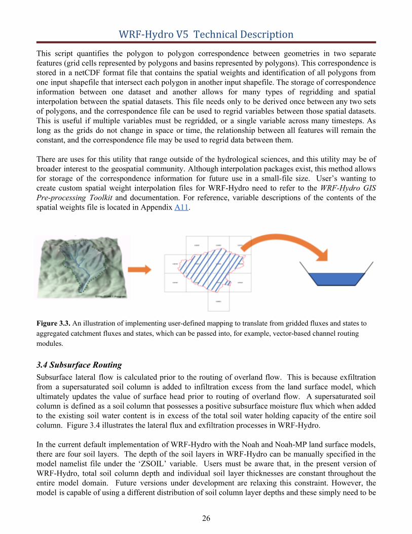
This script quantifies the polygon to polygon correspondence between geometries in two separate features (grid cells represented by polygons and basins represented by polygons). This correspondence is stored in a netCDF format file that contains the spatial weights and identification of all polygons from one input shapefile that intersect each polygon in another input shapefile. The storage of correspondence information between one dataset and another allows for many types of regridding and spatial interpolation between the spatial datasets. This file needs only to be derived once between any two sets of polygons, and the correspondence file can be used to regrid variables between those spatial datasets. This is useful if multiple variables must be regridded, or a single variable across many timesteps. As long as the grids do not change in space or time, the relationship between all features will remain the constant, and the correspondence file may be used to regrid data between them.
There are uses for this utility that range outside of the hydrological sciences, and this utility may be of broader interest to the geospatial community. Although interpolation packages exist, this method allows for storage of the correspondence information for future use in a small-file size. User’s wanting to create custom spatial weight interpolation files for WRF-Hydro need to refer to the WRF-Hydro GIS Pre-processing Toolkit and documentation. For reference, variable descriptions of the contents of the spatial weights file is located in Appendix A11.
Figure 3.3. An illustration of implementing user-defined mapping to translate from gridded fluxes and states to aggregated catchment fluxes and states, which can be passed into, for example, vector-based channel routing modules.
3.4 Subsurface Routing Subsurface lateral flow is calculated prior to the routing of overland flow. This is because exfiltration from a supersaturated soil column is added to infiltration excess from the land surface model, which ultimately updates the value of surface head prior to routing of overland flow. A supersaturated soil column is defined as a soil column that possesses a positive subsurface moisture flux which when added to the existing soil water content is in excess of the total soil water holding capacity of the entire soil column. Figure 3.4 illustrates the lateral flux and exfiltration processes in WRF-Hydro.
In the current default implementation of WRF-Hydro with the Noah and Noah-MP land surface models, there are four soil layers. The depth of the soil layers in WRF-Hydro can be manually specified in the model namelist file under the ‘ZSOIL’ variable. Users must be aware that, in the present version of WRF-Hydro, total soil column depth and individual soil layer thicknesses are constant throughout the entire model domain. Future versions under development are relaxing this constraint. However, the model is capable of using a different distribution of soil column layer depths and these simply need to be
26
WRF-Hydro V5 Technical Description
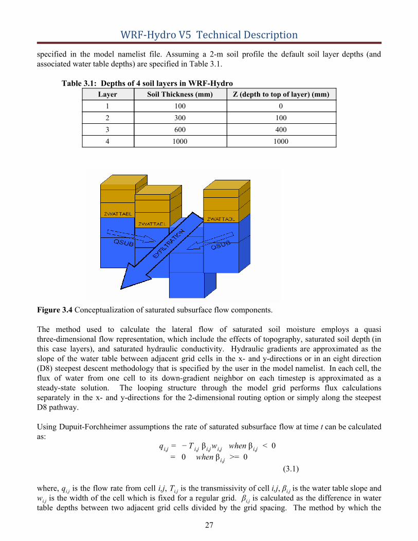
specified in the model namelist file. Assuming a 2-m soil profile the default soil layer depths (and associated water table depths) are specified in Table 3.1.
Table 3.1: Depths of 4 soil layers in WRF-Hydro Layer Soil Thickness (mm) Z (depth to top of layer) (mm)
1 100 0 2 300 100 3 600 400 4 1000 1000
Figure 3.4 Conceptualization of saturated subsurface flow components.
The method used to calculate the lateral flow of saturated soil moisture employs a quasi three-dimensional flow representation, which include the effects of topography, saturated soil depth (in this case layers), and saturated hydraulic conductivity. Hydraulic gradients are approximated as the slope of the water table between adjacent grid cells in the x- and y-directions or in an eight direction (D8) steepest descent methodology that is specified by the user in the model namelist. In each cell, the flux of water from one cell to its down-gradient neighbor on each timestep is approximated as a steady-state solution. The looping structure through the model grid performs flux calculations separately in the x- and y-directions for the 2-dimensional routing option or simply along the steepest D8 pathway.
Using Dupuit-Forchheimer assumptions the rate of saturated subsurface flow at time t can be calculated as:
β w when β 0 qi,j = − T i,j i,j i,j i,j < 0 when β = 0 = i,j >
(3.1)
where, qi,j is the flow rate from cell i,j , Ti,j is the transmissivity of cell i,j , β i,j is the water table slope and w i,j is the width of the cell which is fixed for a regular grid. β i,j is calculated as the difference in water table depths between two adjacent grid cells divided by the grid spacing. The method by which the
27
WRF-Hydro V5 Technical Description
water table depth is determined is provided below. Transmissivity is a power law function of saturated hydraulic conductivity (Ksat i,j) and soil thickness ( Di,j) given by:
T 1 when z = Di,j = ni,j
Ksat Di,j i,j ( −zi,j
Di,j)ni,j
i,j < i,j
0 when z D = i,j > i,j(3.2)
where, zi,j is the depth to the water table. n i,j in Eq. (3.2) is defined as the local power law exponent and is a tunable parameter (currently hard-coded to 1 but will be exposed in future versions) that dictates the rate of decay of Ksati,j with depth. When Eq. (3.2) is substituted into (3.1) the flow rate from cell i,j to its neighbor in the x-direction can be expressed as
(3.3)
where,
γx(i,j) = − ( ni,j
w Ksat Di,j i,j i,j) βx(i,j)(3.4)
(3.5)
This calculation is repeated for the y-direction when using the two-dimensional routing method. The net lateral flow of saturated subsurface moisture ( Qnet) for cell i,j then becomes:
(3.6)
The mass balance for each cell on a model time step (Δt ) can then be calculated in terms of the change in depth to the water table ( Δz ):
(3.7)
where, φ is the soil porosity, R is the soil column recharge rate from infiltration or deep subsurface injection and A is the grid cell area. In WRF-Hydro, R , is implicitly accounted for during the land surface model integration as infiltration and subsequent soil moisture increase. Assuming there is no deep soil injection of moisture (i.e. pressure driven flow from below the lowest soil layer), R, in WRF-Hydro is set equal to 0.
The methodology outlined in Equations 3.2-3.7 has no explicit information on soil layer structure, as the method treats the soil as a single homogeneous column (with an assumed exponential decay of saturated hydraulic conductivity). Therefore, changes in water table depth (Δ z) need to be remapped to the land surface model soil layers. WRF-Hydro specifies the water table depth according the depth of the top of the highest (i.e. nearest to the surface) saturated layer. The residual saturated water above the uppermost,
28
WRF-Hydro V5 Technical Description
saturated soil layer is then added to the overall soil water content of the overlying unsaturated layer. This computational structure requires accounting steps to be performed prior to calculating Qnet.
Given the timescale for groundwater movement and limitations in the model structure there is significant uncertainty in the time it takes to properly spin-up groundwater systems. The main things to consider include 1) the specified depth of soil and number and thickness of the soil vertical layers and 2) the prescription of the model bottom boundary condition. Typically, for simulations with deep soil profiles (e.g. > 10 m) the bottom boundary condition is set to a ‘no-flow’ boundary (SLOPE_DATA = 0.0) in the GENPARM.TBL parameter file (see Appendices A6 and A7, for a description of GENPARM.TBL).
Relevant code modules: Routing/Noah_distr_routing.F
Relevant namelist options: hydro.namelist :
● SUBRTSWCRT - Switch to activate subsurface flow routing.● DXRT - Specification of the routing grid cell spacing● AGGFACTR - Subgrid aggregation factor, defined as the ratio of the subgrid resolution to the
native land model resolution● DTRT_TER - Terrain routing grid time step (used for overland and subsurface routing)
Relevant domain and parameter files/variables: ● TOPOGRAPHY in Fulldom_hires.nc - Terrain grid or Digital Elevation Model (DEM).
Note: this grid may be provided at resolutions equal to or finer than the native land modelresolution.
● LKSATFAC in Fulldom_hires.nc - Multiplier on saturated hydraulic conductivity in lateral flow direction.
● SATDK, SMCMAX, SMCREF in HYDRO.TBL or hydro2dtbl.nc - Soil properties(saturated hydraulic conductivity, porosity, field capacity) used in lateral flow routing.
3.5 Surface Overland Flow Routing Overland flow in WRF-Hydro is calculated using a fully-unsteady, explicit, finite-difference, diffusive wave formulation similar to that of Julien et al. (1995) and Ogden et al. (1997). The diffusive wave equation, while slightly more complicated, is, under some conditions, superior to the simpler and more traditionally used kinematic wave equation, because it accounts for backwater effects and allows for flow on adverse slopes. The overland flow routine described below can be implemented in either a 2-dimensional (x and y direction) or 1-dimension (steepest descent or “D8”) method. While the 2-dimensional method may provide a more accurate depiction of water movement across some complex surfaces it is more expensive in terms of computational time compared with the 1-dimensional method. While the physics of both methods are identical we have presented the formulation of the flow in equation form below using the 2-dimensional methodology.
29
WRF-Hydro V5 Technical Description
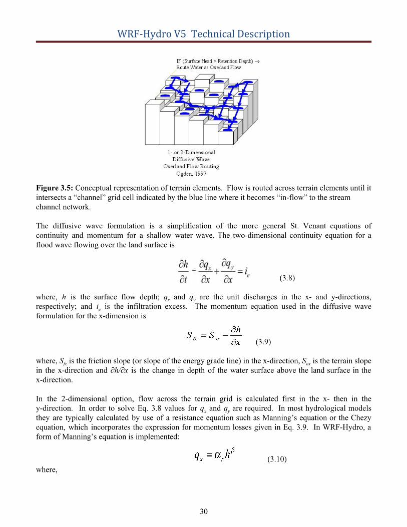
Figure 3.5: Conceptual representation of terrain elements. Flow is routed across terrain elements until it intersects a “channel” grid cell indicated by the blue line where it becomes “in-flow” to the stream channel network.
The diffusive wave formulation is a simplification of the more general St. Venant equations of continuity and momentum for a shallow water wave. The two-dimensional continuity equation for a flood wave flowing over the land surface is
(3.8)
where, h is the surface flow depth; qx and qy are the unit discharges in the x- and y-directions, respectively; and i e is the infiltration excess. The momentum equation used in the diffusive wave formulation for the x-dimension is
(3.9)
where, Sfx is the friction slope (or slope of the energy grade line) in the x-direction, Sox is the terrain slope in the x-direction and ∂h/∂x is the change in depth of the water surface above the land surface in the x-direction.
In the 2-dimensional option, flow across the terrain grid is calculated first in the x- then in the y-direction. In order to solve Eq. 3.8 values for q x and qy are required. In most hydrological models they are typically calculated by use of a resistance equation such as Manning’s equation or the Chezy equation, which incorporates the expression for momentum losses given in Eq. 3.9. In WRF-Hydro, a form of Manning’s equation is implemented:
(3.10) where,
30

WRF-Hydro V5 Technical Description
(3.11)
where, nOV is the roughness coefficient of the land surface and is a tunable parameter and β is a unit dependent coefficient expressed here for SI units.
The overland flow formulation has been used effectively at fine terrain scales ranging from 30-300 m. There has not been rigorous testing to date, in WRF-Hydro, at larger length-scales (> 300 m). This is due to the fact that typical overland flood waves possess length scales much smaller than 1 km. Micro-topography can also influence the behavior of a flood wave. Correspondingly, at larger grid sizes (e.g. > 300 m) there will be poor resolution of the flood wave and the small-scale features that affect it. Also, at coarser resolutions, terrain slopes between grid cells are lower due to an effective smoothing of topography as grid size resolution is decreased. Each of these features will degrade the performance of dynamic flood wave models to accurately simulate overland flow processes. Hence, it is generally considered that finer resolutions yield superior results.
The selected model time step is directly tied to the grid resolution. In order to prevent numerical diffusion of a simulated flood wave (where numerical diffusion is the artificial dissipation and dispersion of a flood wave) a proper time step must be selected to match the selected grid size. This match is dependent upon the assumed wave speed or celerity (c ). The Courant Number, Cn= c(Δt/Δx) , should be close to 1.0 in order to prevent numerical diffusion. The value of the Cn also affects the stability of the routing routine such that values of Cn should always be less than 1.0. Therefore the following model time steps are suggested as a function of model grid size as shown in Table 3.2.
Table 3.2: Suggested routing time steps for various grid spacings X (m) T (s)
30 2 100 6 250 15 500 30
Relevant code modules: Routing/Noah_distr_routing.F
Relevant namelist options: hydro.namelist :
● OVRTSWCRT - Switch to activate overland flow routing.● DXRT - Specification of the routing grid cell spacing● AGGFACTR - Subgrid aggregation factor, defined as the ratio of the subgrid resolution to the
native land model resolution● DTRT_TER - Terrain routing grid time step (used for overland and subsurface routing)
Relevant domain and parameter files/variables: ● TOPOGRAPHY in Fulldom_hires.nc - Terrain grid or Digital Elevation Model (DEM).
Note: this grid may be provided at resolutions equal to or finer than the native land modelresolution.
31
WRF-Hydro V5 Technical Description
● RETDEPRTFAC in Fulldom_hires.nc - Multiplier on maximum retention depth beforeflow is routed as overland flow.
● OVROUGHRTFAC in Fulldom_hires.nc - Multiplier on Manning's roughness foroverland flow.
● OV_ROUGH in HYDRO.TBL or OV_ROUGH2D hydro2dtbl.nc - Manning's roughnessfor overland flow (by default a function of land use type).
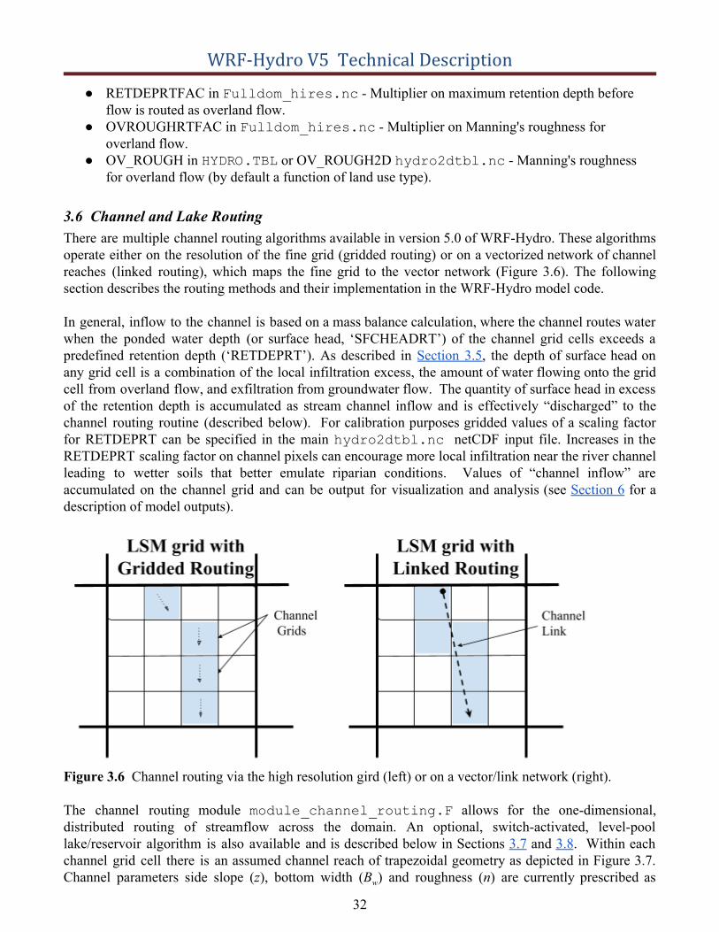
3.6 Channel and Lake Routing There are multiple channel routing algorithms available in version 5.0 of WRF-Hydro. These algorithms operate either on the resolution of the fine grid (gridded routing) or on a vectorized network of channel reaches (linked routing), which maps the fine grid to the vector network (Figure 3.6). The following section describes the routing methods and their implementation in the WRF-Hydro model code.
In general, inflow to the channel is based on a mass balance calculation, where the channel routes water when the ponded water depth (or surface head, ‘SFCHEADRT’) of the channel grid cells exceeds a predefined retention depth (‘RETDEPRT’). As described in Section 3.5, the depth of surface head on any grid cell is a combination of the local infiltration excess, the amount of water flowing onto the grid cell from overland flow, and exfiltration from groundwater flow. The quantity of surface head in excess of the retention depth is accumulated as stream channel inflow and is effectively “discharged” to the channel routing routine (described below). For calibration purposes gridded values of a scaling factor for RETDEPRT can be specified in the main hydro2dtbl.nc netCDF input file. Increases in the RETDEPRT scaling factor on channel pixels can encourage more local infiltration near the river channel leading to wetter soils that better emulate riparian conditions. Values of “channel inflow” are accumulated on the channel grid and can be output for visualization and analysis (see Section 6 for a description of model outputs).
Figure 3.6 Channel routing via the high resolution gird (left) or on a vector/link network (right).
The channel routing module module_channel_routing.F allows for the one-dimensional, distributed routing of streamflow across the domain. An optional, switch-activated, level-pool lake/reservoir algorithm is also available and is described below in Sections 3.7 and 3.8. Within each channel grid cell there is an assumed channel reach of trapezoidal geometry as depicted in Figure 3.7. Channel parameters side slope (z ), bottom width (B w) and roughness (n) are currently prescribed as
32

WRF-Hydro V5 Technical Description
functions of Strahler stream order for defaults. Details on how each routing method reads these parameters are specified in the subsections below.
● Channel Slope, So● Channel Length, (m)● Channel side slope, z (m)● Constant bottom width, Bw (m)● Manning’s roughness coefficient, ( n )
Figure 3.7 Schematic of Channel Routing Terms
As discussed above, channel elements receive lateral inflow from overland flow. There is currently no overbank flow back to the fine-grid, so flow into the channel model is effectively one-way. Therefore, WRF-Hydro does not explicitly represent inundation areas from overbank flow from the channel back to the terrain. This will be an upcoming enhancement, though currently there are methods for post-processing an inundation surface. Uncertainties in channel geometry parameters and the lack of an overbank flow representation result in a measure of uncertainty for users wishing to compare model flood inundation versus those from observations. It is strongly recommended that users compare model versus observed streamflow discharge values and use observed stage-discharge relationships or “rating curves” when wishing to relate modeled/predicted streamflow values to actual river levels and potential inundation areas.
Relevant code modules: Routing/ module_channel_routing.F
Relevant namelist options for gridded and reach-based routing: hydro.namelist :
● CHANRTSWCRT - Switch to activate channel routing.● channel_option - Specification of the type of channel routing to activate● DTRT_CH - Channel routing time step, applies to both gridded and reach-based channel routing
methods● route_link_f (optional) - a Route_Link.nc file is required for reach-based routing methods.
Example header in Appendix A9.
3.6.1. Gridded Routing using Diffusive Wave Channel flow down through the gridded channel network is performed using an explicit, one-dimensional, variable time-stepping diffusive wave formulation. As mentioned above the diffusive
33
WRF-Hydro V5 Technical Description
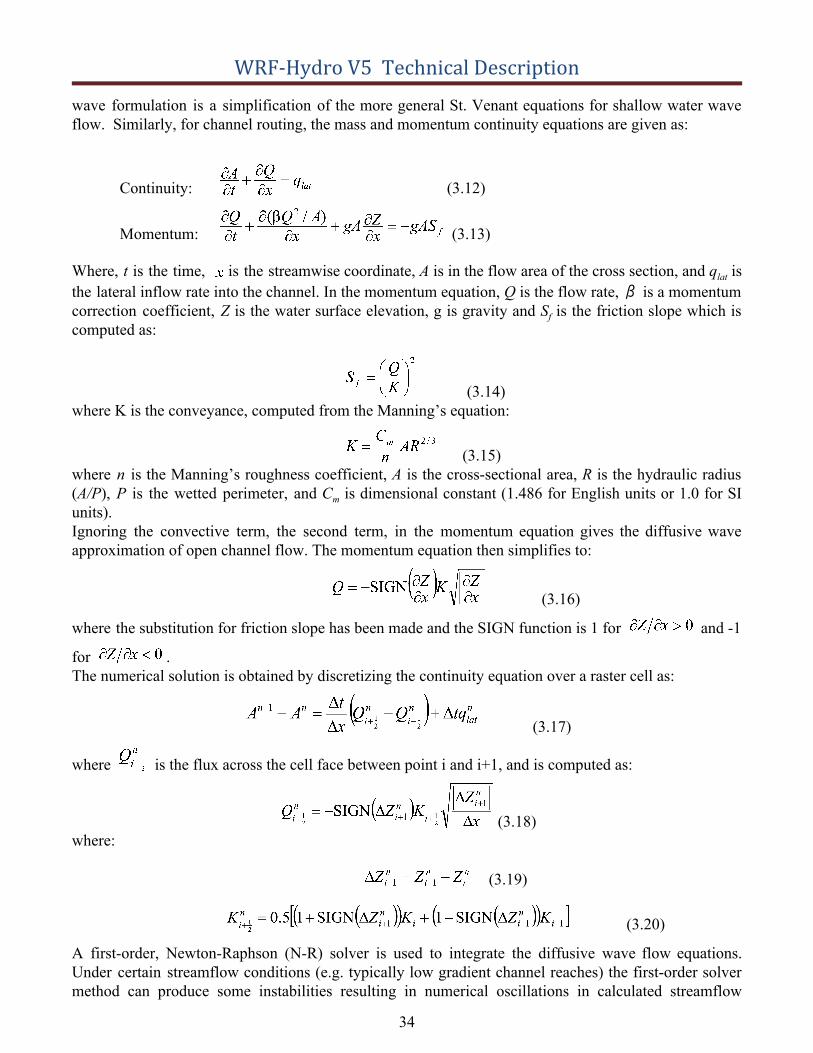
wave formulation is a simplification of the more general St. Venant equations for shallow water wave flow. Similarly, for channel routing, the mass and momentum continuity equations are given as:
Continuity: (3.12)
Momentum: (3.13)
Where, t is the time, is the streamwise coordinate, A is in the flow area of the cross section, and q lat is the lateral inflow rate into the channel. In the momentum equation, Q is the flow rate, β is a momentum correction coefficient, Z is the water surface elevation, g is gravity and S f is the friction slope which is computed as:
(3.14)where K is the conveyance, computed from the Manning’s equation:
(3.15) where n is the Manning’s roughness coefficient, A is the cross-sectional area, R is the hydraulic radius (A/P ), P is the wetted perimeter, and C m is dimensional constant (1.486 for English units or 1.0 for SI units). Ignoring the convective term, the second term, in the momentum equation gives the diffusive wave approximation of open channel flow. The momentum equation then simplifies to:
(3.16)
where the substitution for friction slope has been made and the SIGN function is 1 for and -1
for . The numerical solution is obtained by discretizing the continuity equation over a raster cell as:
(3.17)
where is the flux across the cell face between point i and i+1, and is computed as:
(3.18) where:
(3.19)
(3.20)
A first-order, Newton-Raphson (N-R) solver is used to integrate the diffusive wave flow equations. Under certain streamflow conditions (e.g. typically low gradient channel reaches) the first-order solver method can produce some instabilities resulting in numerical oscillations in calculated streamflow
34
WRF-Hydro V5 Technical Description
values. To address this issue, higher order solver methods will be implemented in future versions of WRF-Hydro.
Unlike typical overland flow flood waves which have very shallow flow depths, on the order of millimeters or less, channel flood waves have appreciably greater flow depths and wave amplitudes, which can potentially result in strong momentum gradients and strong accelerations of the propagating wave. To properly characterize the dynamic propagation of such highly variable flood waves it is often necessary to decrease model time-steps in order to satisfy Courant conditions. Therefore WRF-Hydro utilizes variable time-stepping in the diffusive wave channel routing module in order to satisfy Courant constraints and avoid numerical dispersion and instabilities in the solutions. The initial value of the channel routing time-step is set equal to that of the overland flow routing timestep which is a function of grid spacing. If, during model integration the N-R convergence criteria for upstream-downstream streamflow discharge values is not met, the channel routing time-step is decreased by a factor of one-half and the N-R solver is called again.
It is important to note that use of variable time-stepping can affect model computational performance resulting in slower solution times for rapidly evolving streamflow conditions such as those occurring during significant flood events. Therefore, selection of the time-step decrease factor (default value set to 0.5) and the N-R convergence criteria can each affect model computational performance.
Uncertainty in channel routing parameters can also impact the accuracy of the model solution which implies that model calibration is often required upon implementation in a new domain. Presently, all of the channel routing parameters are prescribed as functions of stream order in a channel routing parameter table CHANPARM.TBL . The structure of this file is described in detail in Appendix A9. It should be noted that prescription of channel flow parameters as functions of stream order is likely to be a valid assumption over relatively small catchments and not over large regions.
3.6.2. Linked Routing using Muskingum and Muskingum-Cunge The gridded catchment and drainage network of the land surface model (Noah/Noah-MP LSM) are mapped to the one-dimensional vectorized channel network, with a unique set of channel properties defined as constant for each reach. The flow out of each channel reach is determined based on flow hydraulics, channel storage and the lateral inflow contribution from each grid cell that is mapped to the individual link element. Since reach lengths are not constant, the number of contributing grid cells to the link depend on the link length (Figure 3.6). Flow is assumed always upstream-to-downstream, and channel junctions accommodate the merging of flows through the linked network. The simultaneous transformation of the often complex drainage network, source areas, and channel flow hydrographs in these large, complex networks necessitates a practical and efficient solution of the routing problem (Brunner and Gorbrecht, 1991).
On the linked network, WRF-Hydro makes use of a fairly standard implementation of the Muskingum-Cunge (MC) method of hydrograph routing which makes use of time varying parameter estimates. The scheme is a practical approach to characterize watershed runoff characteristics over large network, large watershed flow integration. But as a one-dimensional explicit scheme, it does not allow for backwater or localized effects. Channel flows are routed upstream to downstream in a cascade routing manner (Gunner and Gorbetch, 1991) with the assumption that there are negligible backwater effects. The MC routing scheme relates inflow and outflow using a storage relationship, where S = K[XI + (1-X) Q], (3.21) where X is a weighting factor with a range of 0 ≤ X ≤ 0.5, where X range from 0 for
35
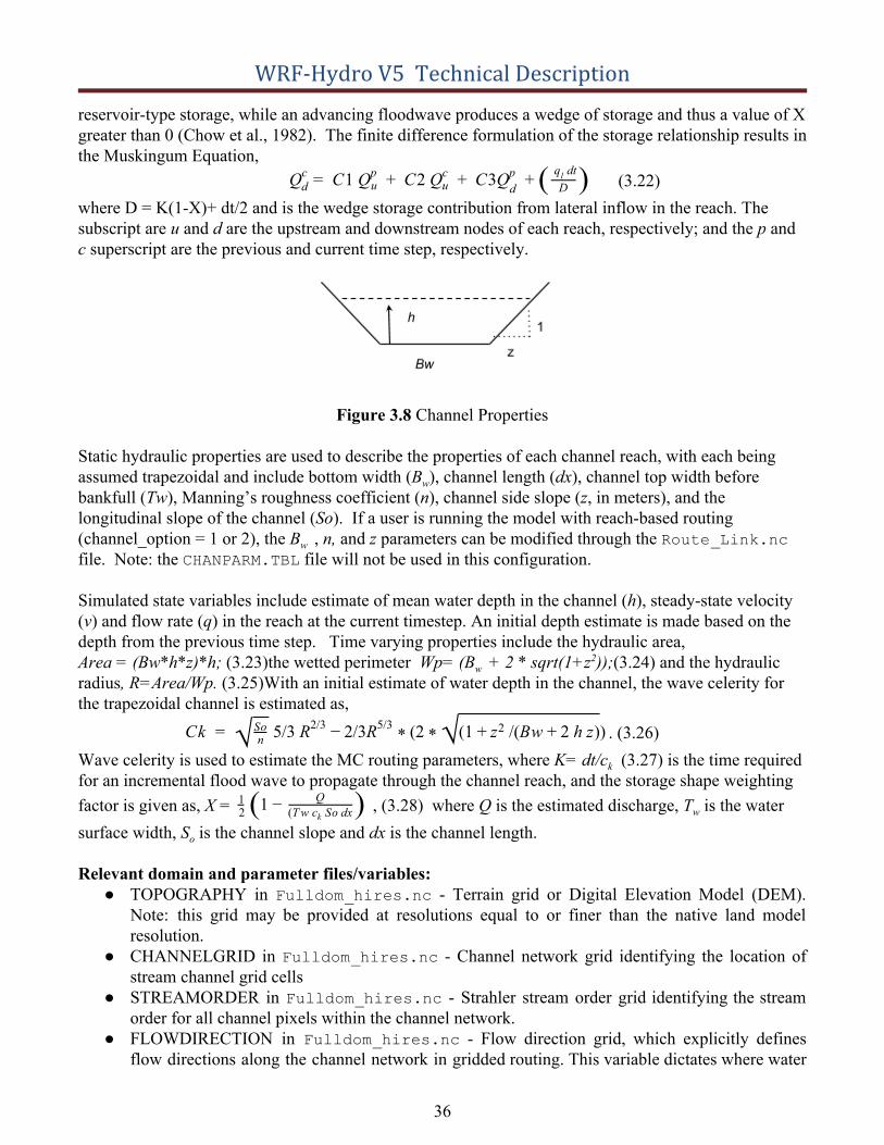
WRF-Hydro V5 Technical Description
reservoir-type storage, while an advancing floodwave produces a wedge of storage and thus a value of X greater than 0 (Chow et al., 1982). The finite difference formulation of the storage relationship results in the Muskingum Equation,
(3.22)C1 Q C2 Q C3QQcd = p
u + cu + p
d + ( D q dtl )
where D = K(1-X)+ dt/2 and is the wedge storage contribution from lateral inflow in the reach. The subscript are u and d are the upstream and downstream nodes of each reach, respectively; and the p and c superscript are the previous and current time step, respectively.
Figure 3.8 Channel Properties
Static hydraulic properties are used to describe the properties of each channel reach, with each being assumed trapezoidal and include bottom width ( Bw), channel length (dx ), channel top width before bankfull (Tw ), Manning’s roughness coefficient ( n), channel side slope ( z, in meters), and the longitudinal slope of the channel ( So). If a user is running the model with reach-based routing (channel_option = 1 or 2), the B w , n, and z parameters can be modified through the Route_Link.ncfile. Note: the CHANPARM.TBL file will not be used in this configuration.
Simulated state variables include estimate of mean water depth in the channel ( h ), steady-state velocity (v) and flow rate ( q) in the reach at the current timestep. An initial depth estimate is made based on the depth from the previous time step. Time varying properties include the hydraulic area, Area = (Bw*h*z)*h; (3.23)the wetted perimeter Wp= (B w + 2 * sqrt(1+z 2)); (3.24) and the hydraulic radius, R=Area/Wp. (3.25)With an initial estimate of water depth in the channel, the wave celerity for the trapezoidal channel is estimated as,
. (3.26)k 5/3 R /3R 2 ) C = √ nSo 2/3 − 2 5/3
* ( * √(1 /(Bw h z)+ z2 + 2 Wave celerity is used to estimate the MC routing parameters, where K= dt/ck (3.27) is the time required for an incremental flood wave to propagate through the channel reach, and the storage shape weighting factor is given as, X = , (3.28) where Q is the estimated discharge, Tw is the water 2
1 1( − Q(T w c So dxk
) surface width, So is the channel slope and dx is the channel length.
Relevant domain and parameter files/variables: ● TOPOGRAPHY in Fulldom_hires.nc - Terrain grid or Digital Elevation Model (DEM).
Note: this grid may be provided at resolutions equal to or finer than the native land model resolution.
● CHANNELGRID in Fulldom_hires.nc - Channel network grid identifying the location of stream channel grid cells
● STREAMORDER in Fulldom_hires.nc - Strahler stream order grid identifying the stream order for all channel pixels within the channel network.
● FLOWDIRECTION in Fulldom_hires.nc - Flow direction grid, which explicitly defines flow directions along the channel network in gridded routing. This variable dictates where water
36
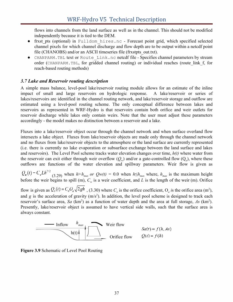
WRF-Hydro V5 Technical Description
flows into channels from the land surface as well as in the channel. This should not be modified independently because it is tied to the DEM.
● frxst_pts (optional) in Fulldom_hires.nc - Forecast point grid, which specified selected channel pixels for which channel discharge and flow depth are to be output within a netcdf point file (CHANOBS) and/or an ASCII timeseries file (frxstpts_out.txt).
● CHANPARM.TBL text or Route_Link.nc netcdf file - Specifies channel parameters by stream order (CHANPARM.TBL , for gridded channel routing) or individual reaches (route_link_f, for reach-based routing methods)
3.7 Lake and Reservoir routing description A simple mass balance, level-pool lake/reservoir routing module allows for an estimate of the inline impact of small and large reservoirs on hydrologic response. A lake/reservoir or series of lakes/reservoirs are identified in the channel routing network, and lake/reservoir storage and outflow are estimated using a level-pool routing scheme. The only conceptual difference between lakes and reservoirs as represented in WRF-Hydro is that reservoirs contain both orifice and weir outlets for reservoir discharge while lakes only contain weirs. Note that the user must adjust these parameters accordingly - the model makes no distinction between a reservoir and a lake.
Fluxes into a lake/reservoir object occur through the channel network and when surface overland flow intersects a lake object. Fluxes from lake/reservoir objects are made only through the channel network and no fluxes from lake/reservoir objects to the atmosphere or the land surface are currently represented (i.e. there is currently no lake evaporation or subsurface exchange between the land surface and lakes and reservoirs). The Level Pool scheme tracks water elevation changes over time, h(t) where water from the reservoir can exit either through weir overflow (Q w) and/or a gate-controlled flow (Qo), where these outflows are functions of the water elevation and spillway parameters. Weir flow is given as
(3.29) when h>hmax or Qw(t) = 0.0 when h≤h max where, h max is the maximum height before the weir begins to spill (m), Cw is a weir coefficient, and L is the length of the weir (m). Orifice
flow is given as , (3.30) where C o is the orifice coefficient, Oa is the orifice area (m2), and g is the acceleration of gravity (m/s2). In addition, the level pool scheme is designed to track each reservoir’s surface area, Sa (km2) as a function of water depth and the area at full storage, As (km2). Presently, lake/reservoir object is assumed to have vertical side walls, such that the surface area is always constant.
Figure 3.9 Schematic of Level Pool Routing
37
WRF-Hydro V5 Technical Description
The following lake/reservoir parameters are required for level-pool routing and are defined in the LAKEPARM.nc parameter file. The GIS pre-processing tool can make either of these files and the model will read the one specified in the hydro.namelist file:
● Weir and Orifice Coefficients ( Co, Cw )● Weir Length, L (m)● Orifice Area, Oa (m2)● Reservoir Area, As (km2)● Maximum reservoir height at full storage, h max (m )
The lake/reservoir flow routing option is activated when lake objects are defined and properly indexed as a data field in the high resolution terrain routing grid file. If lake/reservoir objects are present in the lake grid (and also within the channel network) then routing through those objects will occur if the channel is active AND if channel_option = 3 (gridded routing). Currently, the option to activate/inactivate lakes with channel_option = 1 or = 2 is not developed unless the user is running the NWM configuration. There are several special requirements for the lake grid and channel routing grids when lakes/reservoirs are to be represented and these are discussed in Sections 5.4 and 5.6.
Relevant code modules: Routing/ module_channel_routing.F
Relevant namelist options: hydro.namelist :
● route_lake_f (optional) - Path to lake parameter file to support level-pool reservoir routing methods.
○ Note: as mentioned in the paragraph above, if in the GIS-Preprocessing the user created a “gridded” routing stack for channel_option = 3 (i.e. did not select to create a Route_Link.nc file for channel_option = 1 or = 2) AND specified a lake file (user provided a reservoir/lake input file), then the Fulldom_hires.nc file will populate the LAKEGRID variable. For this case, the user must specify the route_lake_f file.To turn lakes “off” with channel_option = 3, create another set of Fulldom_hires.nc (“domain”) files without a reservoir input file specified.
Relevant domain and parameter files/variables: ● CHANNELGRID in Fulldom_hires.nc - Channel network grid identifying the location of
stream channel grid cells● LAKEGRID in Fulldom_hires.nc (optional) - Specifies lake locations on the channel grid
(for gridded channel routing methods, i.e. channel_option = 3).● Route_Link.nc netCDF file (optional) - Specifies lake associations with channel reaches..
***Inactive for channel_option = 1 and = 2 if UDMP = 0.● LAKEPARM.TBL text or LAKEPARM.nc netCDF file - Specifies lake parameters for each lake
object specified.
38
WRF-Hydro V5 Technical Description
3.8 Conceptual base flow model description Aquifer processes contributing baseflow often operate at depths well below ground surface. As such, there are often conceptual shortcomings in current land surface models in their representation of groundwater processes. Because these processes contribute to streamflow (typically as “baseflow”) a parameterization is often used in order to simulate total streamflow values that are comparable with observed streamflow from gauging stations. Therefore, a switch-activated baseflow module module_GW_baseflow.F has been created which conceptually (i.e. not physically-explicit) represents baseflow contributions to streamflow. This model option is particularly useful when WRF-Hydro is used for long-term streamflow simulation/prediction and baseflow or “low flow” processes must be properly accounted for. Besides potential calibration of the land surface model parameters the conceptual baseflow model does not directly impact the performance of the land surface model scheme. The new baseflow module is linked to WRF-Hydro through the discharge of “deep drainage” from the land surface soil column (sometimes referred to as “underground runoff”).
The baseflow parameterization in WRF-Hydro uses spatially-aggregated drainage from the soil profile as recharge to a conceptual groundwater reservoir (Fig. 3.10). The unit of spatial aggregation is often taken to be that of a catchment or sub-basin within a watershed. Each sub-basin has a groundwater reservoir “bucket” with a conceptual depth and associated conceptual volumetric capacity. The reservoir operates as a simple bucket where outflow (= “baseflow” or “stream inflow”) is estimated using an empirically-derived function of recharge. The functional type and parameters are determined empirically from offline tests using an estimation of baseflow from stream gauge observations and model-derived estimates of bucket recharge provided by WRF-Hydro. Presently, WRF-Hydro uses either a direct output-equals-input "pass-through" relationship or an exponential storage-discharge function for estimating the bucket discharge as a function of a conceptual depth of water in the bucket "exponential bucket". Note that, because this is a highly conceptualized formulation, the depth of water in the bucket in no way infers the actual depth of water in a real aquifer system. However, the volume of water that exists in the bucket needs to be tracked in order to maintain mass conservation. Estimated baseflow discharged from the bucket model is then combined with lateral inflow from overland routing (if active) and input directly into the stream network as channel inflow, as referred to above in Section 3.5. Presently, the total basin baseflow flux to the stream network is equally distributed among all channel pixels within a basin for gridded channel routing options or dumped into the top of the reach to be routed downstream for reach-based methods. Lacking more specific information on regional groundwater basins, the groundwater/baseflow basins in WRF-Hydro are often assumed to match those of the surface topography. However, this is not a strict requirement. Buckets can be derived in a number of ways such as where true aquifers are defined or from a 3rd party hydrographic dataset such as the USGS NHDPlus or Hydrosheds.
39
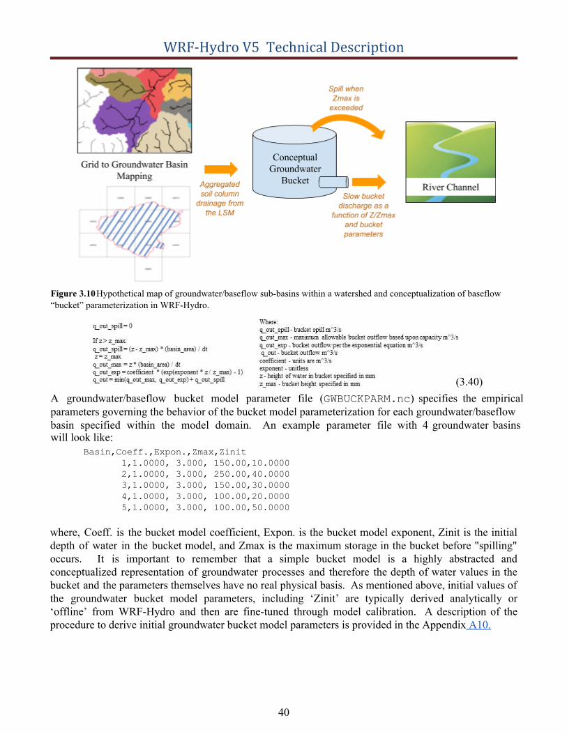
WRF-Hydro V5 Technical Description
Figure 3.10 Hypothetical map of groundwater/baseflow sub-basins within a watershed and conceptualization of baseflow “bucket” parameterization in WRF-Hydro.
A groundwater/baseflow bucket model parameter file (GWBUCKPARM.nc ) specifies the empirical parameters governing the behavior of the bucket model parameterization for each groundwater/baseflow basin specified within the model domain. An example parameter file with 4 groundwater basins will look like:
Basin,Coeff.,Expon.,Zmax,Zinit
1,1.0000, 3.000, 150.00,10.0000
2,1.0000, 3.000, 250.00,40.0000
3,1.0000, 3.000, 150.00,30.0000
4,1.0000, 3.000, 100.00,20.0000
5,1.0000, 3.000, 100.00,50.0000
where, Coeff. is the bucket model coefficient, Expon. is the bucket model exponent, Zinit is the initial depth of water in the bucket model, and Zmax is the maximum storage in the bucket before "spilling" occurs. It is important to remember that a simple bucket model is a highly abstracted and conceptualized representation of groundwater processes and therefore the depth of water values in the bucket and the parameters themselves have no real physical basis. As mentioned above, initial values of the groundwater bucket model parameters, including ‘Zinit’ are typically derived analytically or ‘offline’ from WRF-Hydro and then are fine-tuned through model calibration. A description of the procedure to derive initial groundwater bucket model parameters is provided in the Appendix A10.
40
(3.40)
WRF-Hydro V5 Technical Description
Relevant code modules: Routing/ module_GW_baseflow.F
Relevant namelist options: hydro.namelist:
● GWBASESWCRT - Switch to activate groundwater bucket module.● GWBUCKPARM_file - Path to groundwater bucket parameter file.● gwbasmskfil (optional) - Path to netcdf groundwater basin mask file if using an explicit
groundwater basin 2d grid.● UDMP_OPT (optional) - Switch to activate user-defined mapping between land surface model
grid and conceptual basins.● udmap_file (optional) - If user-defined mapping is active, path to spatial-weights file.
Relevant domain and parameter files/variables: ● GWBUCKPARM.nc netCDF file - Specifies the parameters for each groundwater bucket/basin, in
either text of netCDF format. More information regarding the groundwater bucket modelparameters is provided in Section 5.5 and Appendix A10.
● GWBASINS.nc netCDF file - The 2d grid of groundwater basin IDs.● spatialweights.nc - netCDF file specifying the weights to map between the land surface
grid and the pre-defined groundwater basin boundaries.
41
WRF-Hydro V5 Technical Description
4. Streamflow Nudging Data AssimilationThis chapter describes streamflow nudging and data assimilation in Version 5.0 of WRF-Hydro. Streamflow nudging was introduced in V1.1 of the National Water Model (NWM). The community WRF-Hydro model source code and the NWM source code have merged as of Version 5.0 of WRF-Hydro. See Appendix A16 for more information on the NWM. The chapter is divided into the following sections:
4.1 Streamflow Nudging Data Assimilation Overview 4.2 Nudging Formulation 4.3 Nudging Workflow
4.3.1. Input Files 4.3.2. Output Files
4.4 Nudging compile-time option 4.5 Nudging run-time options
4.1 Streamflow Nudging Data Assimilation Overview For the National Water Model (NWM) , a simple nudging data assimilation (DA) scheme has been developed to correct modeled stream flows to (or towards) observed values. The capability is only currently supported under the NWM configuration, but could be extended to NCAR reach-based routing, and potentially other kinds of routing, in the future. Specifically, the nudging capability introduces an interface for stream discharge observations to be applied to the Muskingum-Cunge streamflow routing solution.
4.2 Nudging Formulation
There are several motivations for performing DA. For the NWM analysis and assimilation cycle, the motivation is to improve model simulation and forecast initial conditions. Nudging is a simple and computationally inexpensive method of data assimilation where an observed state is inserted into the model with some uncertainty. When the observed value is inserted into the model without uncertainty, the method is referred to as “direct insertion”.
Nudging works well locally to observations, both in space and time. Away from observations, in space and time, the method has limited success. For example, our application applies nudging data assimilation on a channel network with the advantage that the corrections are propagated downstream with the network flow. However, if no spatial or temporal smoothing of the corrections are included with the nudging method, upstream errors soon propagate past observed points when in the forecast (away from the observations, in to the future). Various assumptions can be made to smooth the nudge (or correction) in space and/or time but these are highly parameterized and require tuning. In the NWM we have avoided spatial smoothing and have opted to pursue a very limited temporal-interpolation approach.
The basic nudging equation solves e j, the nudge, e, on a spatial element j,
42
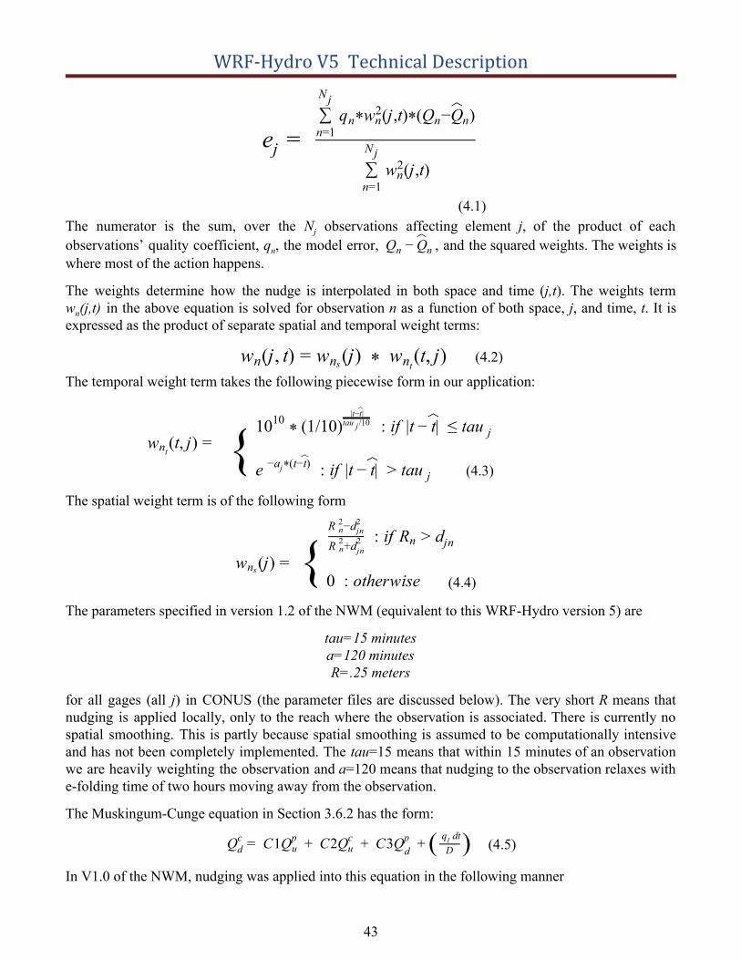
WRF-Hydro V5 Technical Description
ej =(j,t)∑
Nj
n=1w2
n
w (j,t) (Q −Q )∑Nj
n=1qn* 2
n * n︿
n
(4.1) The numerator is the sum, over the N j observations affecting element j , of the product of each observations’ quality coefficient, q n, the model error, , and the squared weights. The weights is Qn − Q
︿
n where most of the action happens.
The weights determine how the nudge is interpolated in both space and time (j,t ). The weights term wn(j,t) in the above equation is solved for observation n as a function of both space, j, and time, t . It is expressed as the product of separate spatial and temporal weight terms:
(4.2)(j, ) (j) w (t, )wn t = wns * ntj
The temporal weight term takes the following piecewise form in our application:
(t, )wntj = { 0 1/10) f |t | au 1 10
* (|t−t|
︿
tau /10j : i − t︿
≤ t j
(4.3) f |t | au e −a (t−t)j*︿
: i − t︿
> t j
The spatial weight term is of the following form
(j)wns = { f RR +d2
n2jn
R −d2n
2jn : i n > djn
(4.4) therwise 0 : o
The parameters specified in version 1.2 of the NWM (equivalent to this WRF-Hydro version 5) are
tau=15 minutes a=120 minutes R=.25 meters
for all gages (all j ) in CONUS (the parameter files are discussed below). The very short R means that nudging is applied locally, only to the reach where the observation is associated. There is currently no spatial smoothing. This is partly because spatial smoothing is assumed to be computationally intensive and has not been completely implemented. The tau=15 means that within 15 minutes of an observation we are heavily weighting the observation and a=120 means that nudging to the observation relaxes with e-folding time of two hours moving away from the observation.
The Muskingum-Cunge equation in Section 3.6.2 has the form:
(4.5)C1Q C2Q C3QQcd = p
u + cu + p
d + ( D q dtl )
In V1.0 of the NWM, nudging was applied into this equation in the following manner
43
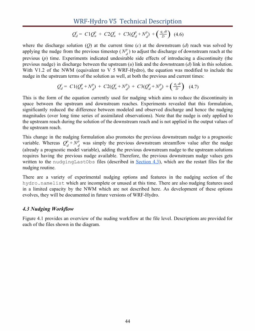
WRF-Hydro V5 Technical Description
(4.6)C1Q C2Q C3(Q ) Qcd = p
u + cu + p
d + N pd + ( D
q dtl )
where the discharge solution (Q ) at the current time (c ) at the downstream (d ) reach was solved by applying the nudge from the previous timestep ( ) to adjust the discharge of downstream reach at the N p
d previous (p ) time. Experiments indicated undesirable side effects of introducing a discontinuity (the previous nudge) in discharge between the upstream (u ) link and the downstream (d ) link in this solution. With V1.2 of the NWM (equivalent to V 5 WRF-Hydro), the equation was modified to include the nudge in the upstream terms of the solution as well, at both the previous and current times:
(4.7)C1(Q ) C2(Q ) C3(Q ) Qcd = p
u + N pd + c
u + N pd + p
d + N pd + ( D
q dtl )
This is the form of the equation currently used for nudging which aims to reduce the discontinuity in space between the upstream and downstream reaches. Experiments revealed that this formulation, significantly reduced the difference between modeled and observed discharge and hence the nudging magnitudes (over long time series of assimilated observations). Note that the nudge is only applied to the upstream reach during the solution of the downstream reach and is not applied in the output values of the upstream reach.
This change in the nudging formulation also promotes the previous downstream nudge to a prognostic variable. Whereas was simply the previous downstream streamflow value after the nudge Qp
d + N pd
(already a prognostic model variable), adding the previous downstream nudge to the upstream solutions requires having the previous nudge available. Therefore, the previous downstream nudge values gets written to the nudgingLastObs files (described in Section 4.3), which are the restart files for the nudging routine.
There are a variety of experimental nudging options and features in the nudging section of the hydro.namelist which are incomplete or unused at this time. There are also nudging features used in a limited capacity by the NWM which are not described here. As development of these options evolves, they will be documented in future versions of WRF-Hydro.
4.3 Nudging Workflow
Figure 4.1 provides an overview of the nuding workflow at the file level. Descriptions are provided for each of the files shown in the diagram.
44
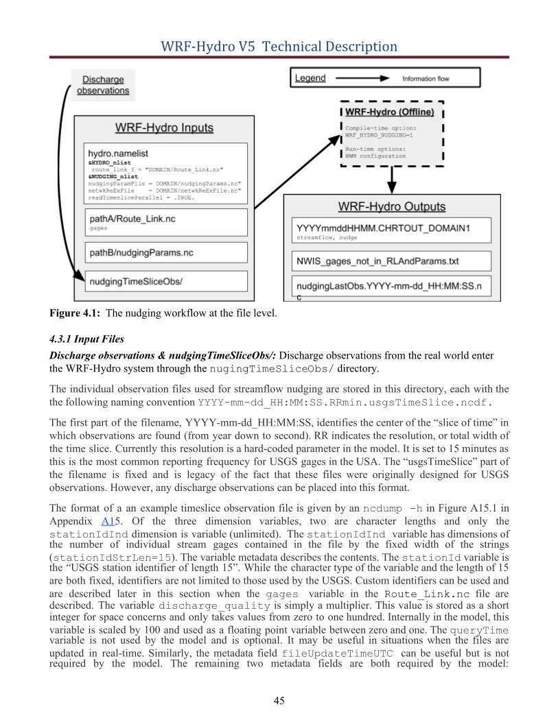
WRF-Hydro V5 Technical Description
Figure 4.1: The nudging workflow at the file level.
4.3.1 Input Files Discharge observations & nudgingTimeSliceObs/: Discharge observations from the real world enter the WRF-Hydro system through the nugingTimeSliceObs/ directory.
The individual observation files used for streamflow nudging are stored in this directory, each with the the following naming convention YYYY-mm-dd_HH:MM:SS.RRmin.usgsTimeSlice.ncdf.
The first part of the filename, YYYY-mm-dd_HH:MM:SS, identifies the center of the “slice of time” in which observations are found (from year down to second). RR indicates the resolution, or total width of the time slice. Currently this resolution is a hard-coded parameter in the model. It is set to 15 minutes as this is the most common reporting frequency for USGS gages in the USA. The “usgsTimeSlice” part of the filename is fixed and is legacy of the fact that these files were originally designed for USGS observations. However, any discharge observations can be placed into this format.
The format of a an example timeslice observation file is given by an ncdump -h in Figure A15.1 in Appendix A15. Of the three dimension variables, two are character lengths and only the stationIdInd dimension is variable (unlimited). The stationIdInd variable has dimensions of the number of individual stream gages contained in the file by the fixed width of the strings (stationIdStrLen=15 ). The variable metadata describes the contents. The stationId variable is the “USGS station identifier of length 15”. While the character type of the variable and the length of 15 are both fixed, identifiers are not limited to those used by the USGS. Custom identifiers can be used and are described later in this section when the gages variable in the Route_Link.nc file are described. The variable discharge_quality is simply a multiplier. This value is stored as a short integer for space concerns and only takes values from zero to one hundred. Internally in the model, this variable is scaled by 100 and used as a floating point variable between zero and one. The queryTime variable is not used by the model and is optional. It may be useful in situations when the files are updated in real-time. Similarly, the metadata field fileUpdateTimeUTC can be useful but is not required by the model. The remaining two metadata fields are both required by the model:
45
WRF-Hydro V5 Technical Description
sliceCenterTimeUTC and sliceTimeResolutionMinutes ensure that the file and the model are operating under the same time location and resolution assumptions. An example of generating timeslice files from USGS observations using the R language is given in the help for the rwrfhydro function WriteNcTimeSlice.
hydro.namelist: When WRF-Hydro is compiled with nudging on, the hydro.namelist file is required to contain the &NUDGING_nlist . The nudging namelist is found at the bottom of the hydro.namelist file either in the Run/ directory after compilation or in the template/HYDRO/ directory. The namelist governs the run-time options to the nudging code. These run-time options are detailed in Section 4.5 below and in Appendix A5.
Route_Link.nc: Collocation of streamflow gages and reach elements is achieved by the gages field in the Route_Link.nc file (see Sections 3.6, 5.4). Each reach element may have a single gage identified with it as specific by a fixed-width 15 character string in the gages field. A blank entry indicates no gage is present on the reach. The gages field in Route_Link.nc tells the nudging module where to apply the observed values to the stream network. Gages which appear in the observation files but not in the Route_Link.nc file do not cause a problem, they are simply skipped and their identifiers collected and printed to the file NWIS_gages_not_in_RLAndParams.txt file, described later. The number of non-blank routelink gages must match the number of gages supplied in the nudging parameters file, described next.
nudgingParams.nc: Figure A15.2 in Appendix A15 shows the structure of the nudgingParams.nc file for a small domain. Some of the parameters in the file are explained in detail in Section 4.2 and some are placeholders for capabilities which have not been developed.
4.3.2 Output Files When the code is compiled with the nudging compile-time option on (see next section), four types of output files contain nudging information. Some files are different than when compiled without nudging while other files are unique outputs for the nuding option.
YYYYmmddHHMM.CHRTOUT_DOMAIN1: The nudging code affects the values written to the “CHRTOUT” files. If valid observations are available, the (modeled) streamflow variable is changed by the assimilated observations. When the model is compiled to enable nudging, the variable “nudge” also appears in the file. The nudge value is calculated as in Section 4.2.
nudgingLastObs.YYYY-mm-dd_HH:MM:SS.nc: These files are unique to the nudging compile and are the restart files for the nudging component of the model. A restart file is not required, nudging can be run from a cold start. This file can contain multiple variables, only the “nudge” variable is described in this documentation.
NWIS_gages_not_in_RLAndParams.txt: These files are unique to nudging and report the unique gages found in the observation time slice files which were not present in the Route_Link.nc file. These are gages which may have opportunity to be assimilated (provided they could be located in the domain). There is only one such file per run, written at the end of the run.
Standard output and “hydro_diag” files: The nudging routines write various messages. The ultimate destination of these can be compiler dependent. The nudging code aims to preface all its messages with “Ndg:” and all its warnings with “Ndg: WARNING:”.
46
WRF-Hydro V5 Technical Description
4.4 Nudging compile-time option
The nuding capability is only available when the code is compiled with the environment variable set: WRF_HYDRO_NUDGING=1 .
4.5 Nudging run-time options Appendix A5 presents an annotated hydro.namelist file. There are two fortran namelists contained within that file. The nudging run-time options are contained the NUDGING_nlist which is the second namelist in the document. Only some run time options listed in the namelist are documented at this time.
Documented/Supported Options Undocumented/Unsupported Options timeSlicePath
nudgingParamFile
nudgingLastObsFile
readTimesliceParallel
temporalPersistence
nLastObs
persistBias
biasWindowBeforeT0
maxAgePairsBiasPersist
minNumPairsBiasPersist
invDistTimeWeightBias
noConstInterfBias
Details on the meaning and usage of the options are given in Appendix A5, in both the comments which are part of the namelist itself and by the blue annotations added to the namelists. The supported options are fairly straight forward in their usage. It is worth noting that the specfication of the nudgingLastObsFile does not behave the same way as the specification of the LSM or hydro restart files. The unsupported nudging options have to do with mostly experimental methods for forecast bias correction which have been investigated.
47
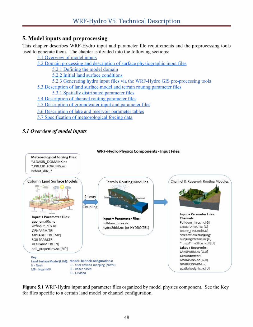
WRF-Hydro V5 Technical Description
5. Model inputs and preprocessingThis chapter describes WRF-Hydro input and parameter file requirements and the preprocessing tools used to generate them. The chapter is divided into the following sections:
5.1 Overview of model inputs 5.2 Domain processing and description of surface physiographic input files
5.2.1 Defining the model domain 5.2.2 Initial land surface conditions 5.2.3 Generating hydro input files via the WRF-Hydro GIS pre-processing tools
5.3 Description of land surface model and terrain routing parameter files 5.3.1 Spatially distributed parameter files
5.4 Description of channel routing parameter files 5.5 Description of groundwater input and parameter files 5.6 Description of lake and reservoir parameter tables 5.7 Specification of meteorological forcing data
5.1 Overview of model inputs
Figure 5.1 WRF-Hydro input and parameter files organized by model physics component. See the Key for files specific to a certain land model or channel configuration.
48
WRF-Hydro V5 Technical Description
WRF-Hydro requires a number of input files describing the model domain, parameters, initial conditions, and when run in a standalone configuration meteorological forcing files. A full list of these files broken up by model physics component is shown in Figure 5.1. Note that the set of files required to run WRF-Hydro varies depending upon model configuration. For example, different land surface models and model physics components may require different parameter and input files.
While some parameter files and templates are included with the model source code, most must be generated by the user. We provide a number of scripts and preprocessing utilities on the WRF-Hydro website (https://ral.ucar.edu/projects/wrf_hydro) in order to aid in this process. These include NCAR Command Language (NCL) scripts to regrid forcing data from commonly used data sources, R scripts to generate parameter and model initialization files, and a set of Python based ArcGIS pre-processing tools. The specific utilities used to generate different files are listed in Table 5.1. Users should be aware that these tools do not support all potential datasets and use cases and that the use of default parameters will often result in suboptimal model performance. More details regarding the pre-processing utilities, file requirements, and descriptions follow.
5.2 Domain processing and description of surface physiographic input files This subsection describes the process of defining the WRF-Hydro model domain, generating model initial conditions, and deriving geospatial input and parameter files via the WRF-Hydro GIS pre-processing tools. As noted in the previous section a number of scripts and utilities have been developed to facilitate the creation of these files. Additionally, we rely on a utility within the Weather Research and Forecasting (WRF) model preprocessing system (WPS) called GEOGRID to define the land surface model grid and relevant geospatial data and produce the resulting geo_em.d0x.nc file hereafter referred to as a “geogrid” file. This geogrid file is then used as input to the ArcGIS preprocessing tools, along with external datasets such as high resolution topographic data, which generate the high resolution routing grid and all surface physiographic input data files required by the model. The geogrid file is also passed to utilities in order to generate land surface model initial condition files.
5.2.1 Defining the model domain The data required to define the domain and geospatial attributes of a spatially-distributed, or gridded, 1-dimensional (vertical) land surface model (LSM) are specified in a geogrid (geo_em.d0x.nc ) netCDF file. This file is generated by the GEOGRID utility in the WRF preprocessing system (WPS). WPS is a preprocessing system that prepares both land surface and atmospheric data for use in the model. The GEOGRID component of WPS automates the procedure of defining in space, georeferencing and attributing most of the land surface parameter data required to execute both the Noah and Noah-MP land surface models. GEOGRID interpolates land surface terrain, soils and vegetation data from standard, readily available data products. These data are distributed as a geographical input data package via the WRF website. Complete documentation and user instructions for use of the WPS system are provided online by NCAR and are updated regularly and, thus, are not discussed in great detail here. This geo_em.d0x.nc file is also required as input to other WRF-Hydro preprocessing utilities.
5.2.2 Initial land surface conditions Initial conditions for the land surface, such as soil moisture, soil temperature, and snow states, are prescribed via the wrfinput_d0x.nc file. This netCDF file can be generated one of two ways,
49

WRF-Hydro V5 Technical Description
through the real.exe program within WRF or via an R script (create_Wrfinput.R ) distributedon the WRF-Hydro website. When created using the real.exe program in WRF, initial conditions arepulled from existing reanalysis or realtime products (see WRF documentation for data and system requirements). This will typically result in more realistic initial model states. However, the process is somewhat involved and requires the user to obtain additional external datasets.
The R script will create a simplified version of the wrfinput (wrfinput_d0x.nc) file including allnecessary fields for the Noah-MP land surface model, but with spatially uniform initial conditions that are prescribed within the script and requires only the geogrid file geo_em.d0x.nc as input. Step-wiseinstructions and detailed requirements are included in documentation distributed with the script. Users should be aware that the model will likely require additional spin-up time when initialized from this file.
5.2.3 Generating hydrologic routing input files via the WRF-Hydro GIS pre-processing tools A suite of Python based utilities, the WRF-Hydro GIS Pre-processing Toolkit , have been developed to facilitate the process of deriving WRF-Hydro input and parameter files from commonly available geospatial data products, such as hydrologically processed digital elevation models. A large number of the hydro input and parameter files described in Table 5.1 can be generated by these tools as well as a geospatial metadata file to support georeferencing of WRF-Hydro model output files and relevant shapefiles to aid in visualizing the model components. The WRF-Hydro GIS pre-processing tools are developed to function as an additional ArcToolbox within the Esri ArcGIS software. Specific operating system and software requirements are addressed in the full WRF-Hydro GIS Pre-processing Toolkit documentation.
The minimum input data requirements for the pre-processing tools are the geogrid file geo_em.d0x.nc and a hydrologically conditioned digital elevation model covering the full extent of the domain of interest. From these datasets the terrain routing Fulldom_hires.nc and channel routing files (seeAppendix A9) can be created. A text file with stream gage locations can also be supplied allowing the user to demarcate these locations in the model input files and optionally produce time series outputs for only these locations frxst_pts_out.txt or *CHANOBS_DOMAINx .
This text file denoting the location of stream gages or forecast points can also be used to generate groundwater input files. Effectively groundwater basins are delineated above each of these locations and default parameters will be assigned to a parameter file that can also be generated using this tool.
Lake and reservoir component input files also require a supplementary input file. A shapefile containing polygons defining the extent of each lake must be provided as input. From this file and the processed digital elevation model a number of parameters are derived for each lake (however, note that other parameters are only assigned a global default value). More details about this process and the contents of the input and parameter files can be found in Appendix A12 and the full WRF-Hydro GIS Pre-processing Toolkit documentation.
The WRF-Hydro GIS Preprocessing Toolkit will also produce a geospatial metadata file for the land surface model grid (as defined by the geogrid file), GEOGRID_LDASOUT_Spatial_Metadata.nc .This file contains projection and coordinate information for the land surface model grid. While this file is an optional input to WRF-Hydro, in combination with the new file output routines in version 5.0.0 of WRF-Hydro this file will allow for the creation of CF (Climate and Forecast metadata convention) compliant output files. This allows for files to be more easily viewed in GIS systems (e.g. ArcGIS and
50
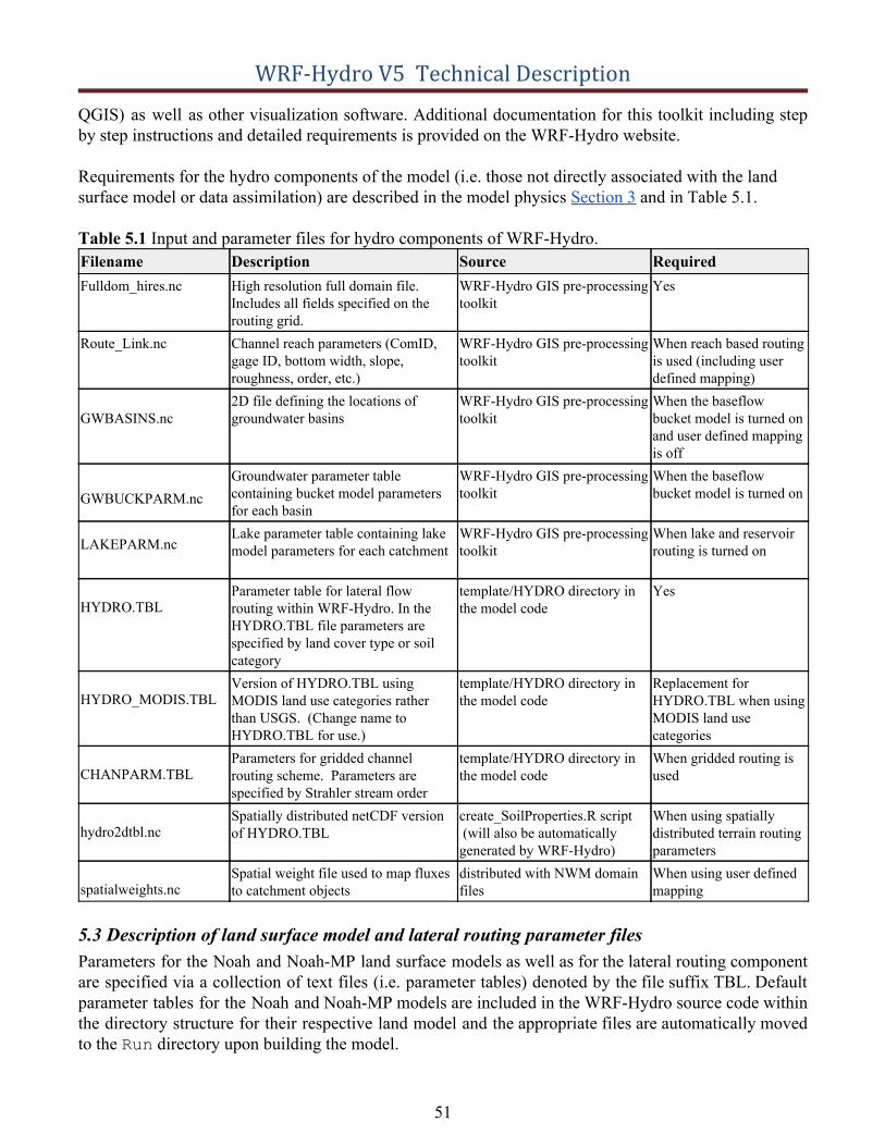
WRF-Hydro V5 Technical Description
QGIS) as well as other visualization software. Additional documentation for this toolkit including step by step instructions and detailed requirements is provided on the WRF-Hydro website.
Requirements for the hydro components of the model (i.e. those not directly associated with the land surface model or data assimilation) are described in the model physics Section 3 and in Table 5.1.
Table 5.1 Input and parameter files for hydro components of WRF-Hydro. Source Required WRF-Hydro GIS pre-processing toolkit
Yes
WRF-Hydro GIS pre-processing toolkit
When reach based routing is used (including user defined mapping)
WRF-Hydro GIS pre-processing toolkit
When the baseflow bucket model is turned on and user defined mapping is off
WRF-Hydro GIS pre-processing toolkit
When the baseflow bucket model is turned on
WRF-Hydro GIS pre-processing toolkit
When lake and reservoir routing is turned on
template/HYDRO directory in the model code
Yes
template/HYDRO directory in the model code
Replacement for HYDRO.TBL when using MODIS land use categories
template/HYDRO directory in the model code
When gridded routing is used
create_SoilProperties.R script (will also be automatically generated by WRF-Hydro)
When using spatially distributed terrain routing parameters
Filename Fulldom_hires.nc
Route_Link.nc
GWBASINS.nc
GWBUCKPARM.nc
LAKEPARM.nc
HYDRO.TBL
HYDRO_MODIS.TBL
CHANPARM.TBL
hydro2dtbl.nc
spatialweights.nc
Description High resolution full domain file. Includes all fields specified on the routing grid. Channel reach parameters (ComID, gage ID, bottom width, slope, roughness, order, etc.) 2D file defining the locations of groundwater basins
Groundwater parameter table containing bucket model parameters for each basin Lake parameter table containing lake model parameters for each catchment
Parameter table for lateral flow routing within WRF-Hydro. In the HYDRO.TBL file parameters are specified by land cover type or soil category Version of HYDRO.TBL using MODIS land use categories rather than USGS. (Change name to HYDRO.TBL for use.) Parameters for gridded channel routing scheme. Parameters are specified by Strahler stream order Spatially distributed netCDF version of HYDRO.TBL
Spatial weight file used to map fluxes to catchment objects
distributed with NWM domain files
When using user defined mapping
5.3 Description of land surface model and lateral routing parameter files Parameters for the Noah and Noah-MP land surface models as well as for the lateral routing component are specified via a collection of text files (i.e. parameter tables) denoted by the file suffix TBL. Default parameter tables for the Noah and Noah-MP models are included in the WRF-Hydro source code within the directory structure for their respective land model and the appropriate files are automatically moved to the Run directory upon building the model.
51
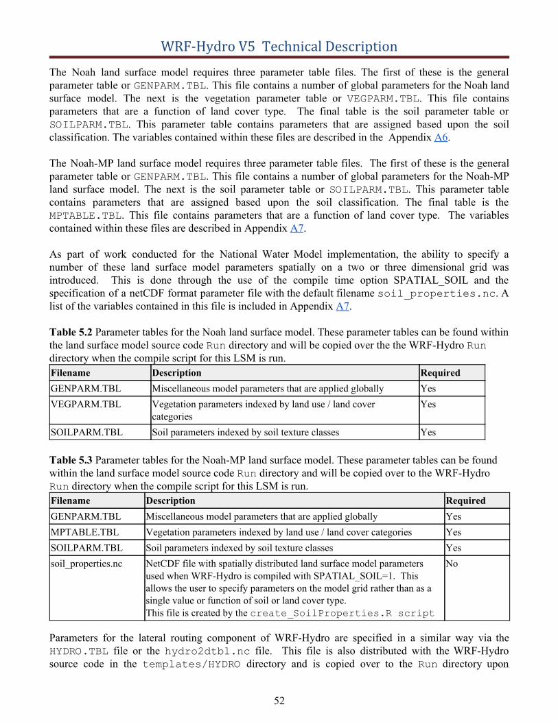
WRF-Hydro V5 Technical Description
The Noah land surface model requires three parameter table files. The first of these is the general parameter table or GENPARM.TBL. This file contains a number of global parameters for the Noah land surface model. The next is the vegetation parameter table or VEGPARM.TBL. This file contains parameters that are a function of land cover type. The final table is the soil parameter table or SOILPARM.TBL . This parameter table contains parameters that are assigned based upon the soil classification. The variables contained within these files are described in the Appendix A6.
The Noah-MP land surface model requires three parameter table files. The first of these is the general parameter table or GENPARM.TBL. This file contains a number of global parameters for the Noah-MP land surface model. The next is the soil parameter table or SOILPARM.TBL . This parameter table contains parameters that are assigned based upon the soil classification. The final table is the MPTABLE.TBL. This file contains parameters that are a function of land cover type. The variables contained within these files are described in Appendix A7.
As part of work conducted for the National Water Model implementation, the ability to specify a number of these land surface model parameters spatially on a two or three dimensional grid was introduced. This is done through the use of the compile time option SPATIAL_SOIL and the specification of a netCDF format parameter file with the default filename soil_properties.nc. A list of the variables contained in this file is included in Appendix A7.
Table 5.2 Parameter tables for the Noah land surface model. These parameter tables can be found within the land surface model source code Run directory and will be copied over the the WRF-Hydro Rundirectory when the compile script for this LSM is run. Filename Description Required GENPARM.TBL Miscellaneous model parameters that are applied globally Yes VEGPARM.TBL Vegetation parameters indexed by land use / land cover
categories Yes
SOILPARM.TBL Soil parameters indexed by soil texture classes Yes
Table 5.3 Parameter tables for the Noah-MP land surface model. These parameter tables can be found within the land surface model source code Run directory and will be copied over to the WRF-HydroRun directory when the compile script for this LSM is run.Filename Description Required GENPARM.TBL Miscellaneous model parameters that are applied globally Yes MPTABLE.TBL Vegetation parameters indexed by land use / land cover categories Yes SOILPARM.TBL Soil parameters indexed by soil texture classes Yes soil_properties.nc NetCDF file with spatially distributed land surface model parameters
used when WRF-Hydro is compiled with SPATIAL_SOIL=1. This allows the user to specify parameters on the model grid rather than as a single value or function of soil or land cover type. This file is created by the create_SoilProperties.R script
No
Parameters for the lateral routing component of WRF-Hydro are specified in a similar way via the HYDRO.TBL file or the hydro2dtbl.nc file. This file is also distributed with the WRF-Hydro source code in the templates/HYDRO directory and is copied over to the Run directory upon
52

WRF-Hydro V5 Technical Description
building the model. There is also an additional HYDRO_MODIS.TBL file for those using the MODIS land cover classification scheme.
The HYDRO.TBL parameter table file contains 2 parts. The first part contains the Manning’s roughness coefficients for overland flow as a function of the USGS vegetation types as that data is used in the Noah land surface model. The roughness values are strictly indexed to the USGS vegetation classes so that if one wanted to use a different vegetation index dataset (e.g. the MODIS/IGBP option in the Noah land surface model) a user would need to remap these roughness values to those new vegetation indices. Users can alter the values of overland flow roughness here for a given vegetation type. However, users may also ‘scale’ these initial values of roughness by changing the gridded values of the overland flow roughness scaling factor (OVROUGHRTFAC) that are contained within the high resolution routing data netCDF file. Because hydrological models are often calibrated over a particular region or watershed as opposed to a specific vegetation type it is recommended that users modify the OVROUGHRTFAC scaling factor as opposed to altering the roughness values in HYDRO.TBL.
The second part of the HYDRO.TBL parameter table contains several soil hydraulic parameters that are classified as functions of soil type. These soil parameters are copied from the SOILPARM.TBL parameter table from the Noah land surface model. They are provided in HYDRO.TBL to allow the user to modify those parameters as needed during model calibration activities without modifying the SOILPARM.TBL file and thus is just done for convenience. In effect, when routing options in WRF-Hydro are activated the code will read the soil hydraulic parameters from HYDRO.TBL. If the Noah land surface model is run within WRF-Hydro without any of the routing options active, the code will simply use the parameter values specific in HYDRO.TBL.
The hydro2dtbl.nc is a spatially distributed netCDF file version of the HYDRO.TBL parameter table. This netCDF file can be created via the create_SoilProperties.R script distributed on the WRF-Hydro website (https://ral.ucar.edu/projects/wrf_hydro ) or will automatically be generated by the model from the HYDRO.TBL if the filename specified in the hydro.namelist does not already exist. See Appendix A8 for further explanation of the variables in the HYDRO.TBL and hydro2dtbl.n c files.
5.3.1 Spatially distributed parameter files
In version 5.0.0 of WRF-Hydro we now allow for the specification of a number of spatially distributed land surface model and / or lateral routing parameters in netCDF input files soil_properties.nc and hydro2dtbl.nc. This option was implemented as part of work conducted for the National Water Model and allows the user to specify parameters on the model grid rather than as a single value or function of soil or land cover type. The files can be generated via an R script provided on our website (create_SoilProperties.R) and are described in more detail in Appendices A7and A8. In order for the model to read in the soil_properties.nc file the SPATIAL_SOIL environment variable must be set to 1 at compile time. This option gives users more flexibility in the specification of land surface model parameters and is particularly useful in the context of calibration and parameter regionalization.
5.4 Description of channel routing parameter files Channel parameters for WRF-Hydro are specified in one of two files. If the model is configured using gridded channel routing these parameters will be stored in CHANPARM.TBL . If the model is configured
53
WRF-Hydro V5 Technical Description
using reach based routing (including the NWM configuration) the parameters and channel geometry are specified within the Route_Link.nc file generated by the WRF-Hydro GIS Pre-processing Toolkit . Variables of the CHANPARM.TBL and Route_Link.nc files are described in Appendix A9.
It is important to keep in mind that there is large uncertainty associated with these parameters. Therefore, model calibration is almost always warranted. Also, because fully-distributed estimates of flow depth (HLINK) are not available for model initialization, it is almost always necessary to use a small initial value of HLINK and let the model come to its own equilibrium (i.e. “spin-up”) after several hours of integration. The necessary time required to spin up the channel network is a direct function of how dense and long your channel network is. Larger, more dense networks will take substantially longer to spin up. Estimates of total travel time from the furthest channel element to the basin outline are a reasonable initial approximation of the time it will take to spin up the channel elements.
5.5 Description of groundwater input and parameter files Depending upon the choice of channel configuration groundwater input and parameter files are specified in slightly different ways. For the National Water Model (NWM) implementation of the model where user defined mapping is active the spatialweights.nc file is used to map gridded fluxes to the appropriate catchments, the spatial unit of the NWM groundwater bucket model. In other configurations of the model where user defined mapping is not used, grid-based groundwater basins are defined in the GWBASINS.nc netCDF file. The contents of these files are described in Appendix A10.Groundwater bucket model parameters are assigned via the GWBUCKPARM.nc file for all configurations. The contents of these files are also summarized in Appendix A10 and like the groundwater basins files these files are produced by the WRF-Hydro GIS Pre-processing Toolkit . Note that global default parameters are prescribed when these files are generated so user adjustments and/or calibration are recommended.
5.6 Description of lake and reservoir parameter tables
Lake parameter values are specified for each one of the lake objects. Typically, baseline parameters are derived within the high-resolution terrain preprocessing stages described above using tools such as ArcGIS (e.g. LkArea, LkMxE). Values for the weir and orifice coefficients and sizes can be drawn from standard engineering hydraulics textbooks (e.g. Chow et al., 1957) and calibrated based on lake level performance. Weir parameters are specified for reservoir “overflow” or “spill” and orifice parameters are specified for design operations. The behavior of the reservoir to store and release water is highly dependent on these parameters and therefore it is highly recommended that the user modify this file with their own set of parameters beyond the default given in the WRF-Hydro GIS Pre-processing Toolkit . See Appendix A12 for descriptions of the variables within the LAKEPARM.nc file.
54

WRF-Hydro V5 Technical Description
5.7 Specification of meteorological forcing data Modern land surface hydrology models, including WRF-Hydro, require meteorological forcing data to simulate land-atmosphere exchanges and terrestrial hydrologic processes when uncoupled to atmospheric modeling systems. Most land models require a similar set of input variables with some variation in terms of the units, spectral bandwidths of radiation, handling of precipitation phase, etc. Most commonly these variables include: incoming short and longwave radiation, humidity, temperature, pressure, wind speed and precipitation. The required variables for the Noah and Noah-MP land surface models supported in version 5.0.0 of WRF-Hydro are listed in Table 5.4. These variables names, units, and several of the forcing data file format options described below are borrowed from the High-Resolution Land Data Assimilation System ( HRLDAS), an offline driver for Noah land surface models. When WRF-Hydro is coupled into other modeling architectures such as the NASA Land Information System (LIS), these systems will set the requirements for the forcing data.
Table 5.4 Input forcing data for the Noah and Noah-MP land surface models Variable name Description Units SWDOWN Incoming shortwave radiation W/m2
LWDOWN Incoming longwave radiation W/m2
Q2D Specific humidity kg/kg T2D Air temperature K PSFC Surface pressure Pa U2D Near surface wind in the u-component m/s V2D Near surface wind in the v-component m/s RAINRATE Precipitation rate mm/s or kg/m2/s
Here we simply describe the requirements and options that are available in the standalone version of WRF-Hydro. Presently, there are 7 forcing data input types in WRF-Hydro. Because it is untenable to support a large variety of input file formats and data types within the model, WRF-Hydro requires that most processing of forcing data be handled external to the model (i.e. as a “pre-process”) and that users put their forcing data into one of the required formats. This includes performing tasks like, gridding of station observations, making sure forcing data is gridded to match the domain grid and has the correct variable names and units (see Table 5.4), reformatting data into the prescribed netCDF format, etc. To facilitate these pre-processing activities we have developed numerous scripts which can be executed to help in the forcing data preparation process. These scripts along with sample data files are distributed on the WRF-Hydro website.
The input forcing data type is specified in the land surface model namelist file namelist.hrldas bymodifying the ‘FORC_TYP’ namelist option. Model forcing type namelist options are specified as follows:
1=HRLDAS-hr format 2=HRLDAS-min format 3=WRF output 4=Idealized 5=Idealized with specified precipitation 6=HRLDAS-hr format with specified precipitation 7=WRF output with specified precipitation
55
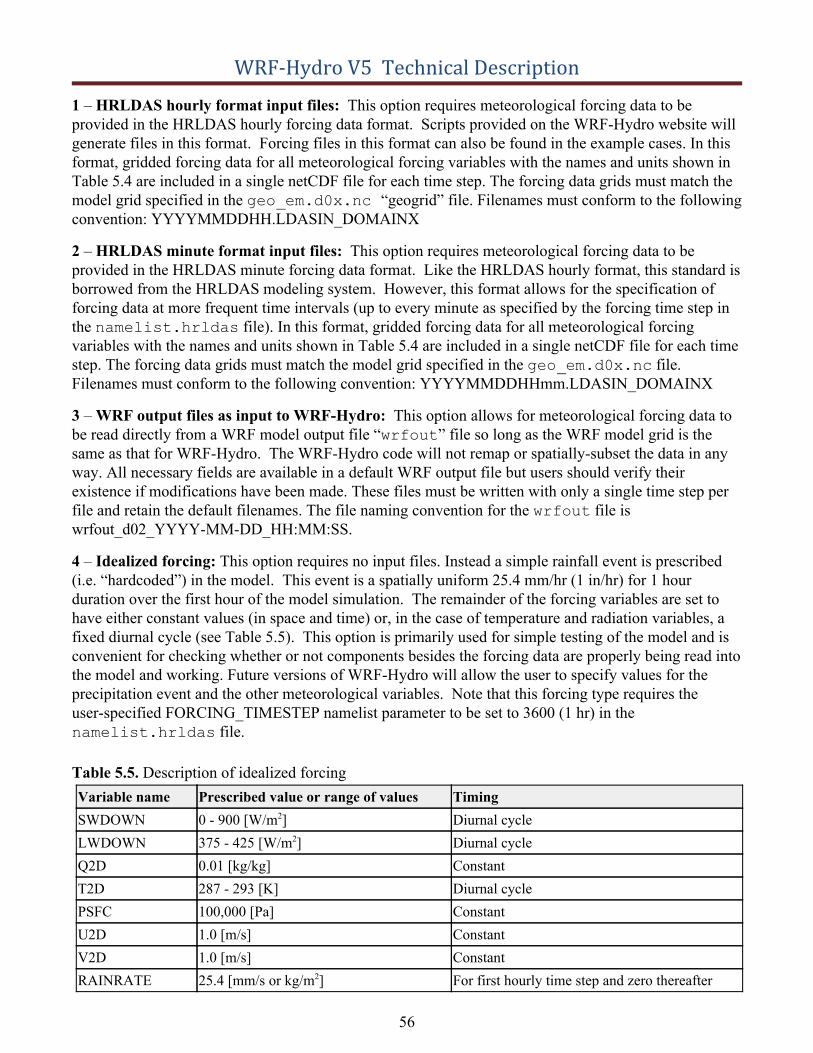
WRF-Hydro V5 Technical Description
1 – HRLDAS hourly format input files: This option requires meteorological forcing data to be provided in the HRLDAS hourly forcing data format. Scripts provided on the WRF-Hydro website will generate files in this format. Forcing files in this format can also be found in the example cases. In this format, gridded forcing data for all meteorological forcing variables with the names and units shown in Table 5.4 are included in a single netCDF file for each time step. The forcing data grids must match the model grid specified in the geo_em.d0x.nc “geogrid” file. Filenames must conform to the followingconvention: YYYYMMDDHH.LDASIN_DOMAINX
2 – HRLDAS minute format input files: This option requires meteorological forcing data to be provided in the HRLDAS minute forcing data format. Like the HRLDAS hourly format, this standard is borrowed from the HRLDAS modeling system. However, this format allows for the specification of forcing data at more frequent time intervals (up to every minute as specified by the forcing time step in the namelist.hrldas file). In this format, gridded forcing data for all meteorological forcingvariables with the names and units shown in Table 5.4 are included in a single netCDF file for each time step. The forcing data grids must match the model grid specified in the geo_em.d0x.nc file.Filenames must conform to the following convention: YYYYMMDDHHmm.LDASIN_DOMAINX
3 – WRF output files as input to WRF-Hydro: This option allows for meteorological forcing data to be read directly from a WRF model output file “ wrfout” file so long as the WRF model grid is thesame as that for WRF-Hydro. The WRF-Hydro code will not remap or spatially-subset the data in any way. All necessary fields are available in a default WRF output file but users should verify their existence if modifications have been made. These files must be written with only a single time step per file and retain the default filenames. The file naming convention for the wrfout file iswrfout_d02_YYYY-MM-DD_HH:MM:SS.
4 – Idealized forcing: This option requires no input files. Instead a simple rainfall event is prescribed (i.e. “hardcoded”) in the model. This event is a spatially uniform 25.4 mm/hr (1 in/hr) for 1 hour duration over the first hour of the model simulation. The remainder of the forcing variables are set to have either constant values (in space and time) or, in the case of temperature and radiation variables, a fixed diurnal cycle (see Table 5.5). This option is primarily used for simple testing of the model and is convenient for checking whether or not components besides the forcing data are properly being read into the model and working. Future versions of WRF-Hydro will allow the user to specify values for the precipitation event and the other meteorological variables. Note that this forcing type requires the user-specified FORCING_TIMESTEP namelist parameter to be set to 3600 (1 hr) in the namelist.hrldas file.
Table 5.5. Description of idealized forcing Variable name Prescribed value or range of values Timing SWDOWN 0 - 900 [W/m2] Diurnal cycle LWDOWN 375 - 425 [W/m2] Diurnal cycle Q2D 0.01 [kg/kg] Constant T2D 287 - 293 [K] Diurnal cycle PSFC 100,000 [Pa] Constant U2D 1.0 [m/s] Constant V2D 1.0 [m/s] Constant RAINRATE 25.4 [mm/s or kg/m2] For first hourly time step and zero thereafter
56
WRF-Hydro V5 Technical Description
5 – Idealized forcing with specified precipitation: This option is identical to forcing type 4 with the exception that the WRF-Hydro system will look for user provided supplementary precipitation files. These supplementary precipitation files are netCDF files containing a single gridded field with either the name “precip” and units of mm or “precip_rate” with unit a unit of mm/s. When using this forcing type, the WRF-Hydro system will look for a new precipitation input file based on the user-specified FORCING_TIMESTEP namelist option set in the namelist.hrldas file. Scripts provided on theWRF-Hydro website will generate files in this format (specifically the MRMS regridding scripts). Forcing files in this format can also be found in the example test cases. Filenames for supplemental precipitation files must conform to this convention: YYYYMMDDHHMM. PRECIP_FORCING.nc.
6 – HRLDAS hourly format input files with specified precipitation: This option is identical to forcing type 1 with the exception that the WRF-Hydro system will also look for user provided supplementary precipitation files. These supplementary precipitation files are netCDF files containing a single gridded field with either the name “precip” and units of mm or “precip_rate” with unit a unit of mm/s. When using this forcing type, the WRF-Hydro system will look for a new precipitation input file based on the user-specified FORCING_TIMESTEP namelist option set in the namelist.hrldasfile. Scripts provided on the WRF-Hydro website will generate files in this format (specifically the MRMS regridding scripts). Forcing files in this format can also be found in the example test cases. Filenames for supplemental precipitation files must conform to this convention: YYYYMMDDHHMM. PRECIP_FORCING.nc.
This option is useful when combining atmospheric analyses from reanalysis products or other models with a separate analysis of precipitation (e.g. a gridded gauge product, radar QPE, nowcasts, satellite QPE, etc). The model reads in the meteorological forcing data fields on each hour and then holds those values constant for the entire hour. Precipitation can be read in more frequently based on the user-specified FORCING_TIMESTEP namelist parameter in the namelist.hrldas file. Forexample, the user can have ‘hourly’ meteorology with ‘5-minute’ precipitation analyses.
7 – WRF output files as input to WRF-Hydro with specified precipitation: This option is identical to forcing type 3 with the exception that the WRF-Hydro system will also look for user provided supplementary precipitation files. These supplementary precipitation files are netCDF files containing a single gridded field with either the name “precip” and units of mm or “precip_rate” with unit a unit of mm/s. When using this forcing type, the WRF-Hydro system will look for a new precipitation input file based on the user-specified FORCING_TIMESTEP namelist option set in the namelist.hrldasfile. Scripts provided on the WRF-Hydro website will generate files in this format (specifically the MRMS regridding scripts). Forcing files in this format can also be found in the example test cases. Filenames for supplemental precipitation files must conform to this convention: YYYYMMDDHHMM. PRECIP_FORCING.nc.
This option is useful when combining forcing data from WRF with a separate analysis of precipitation (e.g. a gridded gauge product, radar QPE, nowcasts, satellite QPE, etc). The model reads in the meteorological forcing data fields from the WRF output file and then holds those values constant until the next file is available. Precipitation can be read in more frequently based on the user-specified FORCING_TIMESTEP namelist parameter in the namelist.hrldas file. For example, the user canhave ‘hourly’ meteorology with ‘5-minute’ precipitation analyses.
57
WRF-Hydro V5 Technical Description
6. Description of Output Files from WRF-HydroThis chapter describes the output files from Version 5.0 of WRF-Hydro.
The user has several options to allow flexibility when outputting from the WRF-Hydro modeling system. All of the options to control outputs are located in the hydro.namelist file that the useredits prior to running a simulation. Prior to turning specific file options on, there are a few high-level namelist options (flags) that help control the quantity of variables each file will produce, along with some flexibility on the level of compression files contain.
io_form_outputs: This flag directs the output to utilize optional internal netCDF compression and the use of optional scale_factor/add_offset attributes to pack variables from floating point to integer. However, the user also has flexibility to turn these optional features off. For additional information on these “packing” attributes, consult the netCDF documentation for a more in-depth explanation (http://www.unidata.ucar.edu/software/netcdf/docs/index.html ). It should be noted that the use of internal compression adds time to output files being produced. This may become costly for large-scale modeling applications. Tests have indicated a cost of 15-25% additional time spent producing output variables when internal netCDF compression is utilized, depending on the number of output files being produced. However, without the use of compression, it is possible file sizes could become large depending on the application. It is also important to note that a value of ‘0’ will result in the code deferring to old output routines used in version 3.0 of WRF-Hydro. For these outputs, the user is encouraged to read the documentation for that version of the code. The following values for the io_form_outputs option are available:
0 - Defer to old output routines for version 3.0 of WRF-Hydro (NOTE: this is the ONLY option that is supported when running with the Noah LSM) 1 - Utilize internal netCDF compression in conjunction with scale_factor/add_offset byte packing 2 - Utilize scale_factor/add_offset byte packing without internal netCDF compression 3 - Utilize internal netCDF compression without scale_factor/add_offset byte packing. 4 - No internal netCDF compression and no scale_factor/add_offset byte packing.
io_config_outputs: This flag offers different sets of output variables for each file. This offers the user some flexibility to the number of output variables being produced. NOTE: This flag has no effect when io_form_outputs = 0.
t0OutputFlag: This flag controls if output files are produced on the initial timestep of the model simulation. It is important to note some variables are initialized to missing values and may translate to missing values in the output files for the initial time step. However, these files may offer useful information to the user for diagnosing purposes.
output_channelBucket_influx: This flag controls the creation of output variables specific to running a channel-only configuration of the model. These variables provide useful information on flow coming into channel links located in the simulation domain, which can be used for diagnosing purposes. Note: this value must be zero for running a gridded channel routing configuration of the model.
An overview of available model output files is shown in Figure 6.1. For a detailed table of each variable contained within each output file, see the WRF-Hydro Output Variable Matrix V 5 located on our website (https://ral.ucar.edu/projects/wrf_hydro) for details. There is no optimal combination of namelist options
58
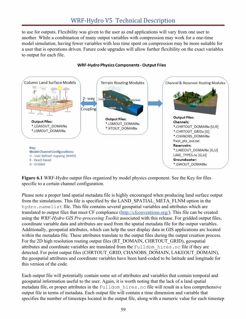
WRF-Hydro V5 Technical Description
to use for outputs. Flexibility was given to the user as end applications will vary from one user to another. While a combination of many output variables with compression may work for a one-time model simulation, having fewer variables with less time spent on compression may be more suitable for a user that is operations driven. Future code upgrades will allow further flexibility on the exact variables to output for each file.
Figure 6.1 WRF-Hydro output files organized by model physics component. See the Key for files specific to a certain channel configuration.
Please note a proper land spatial metadata file is highly encouraged when producing land surface output from the simulations. This file is specified by the LAND_SPATIAL_META_FLNM option in the hydro.namelist file. This file contains several geospatial variables and attributes which aretranslated to output files that meet CF compliance ( http://cfconventions.org/ ). This file can be created using the WRF-Hydro GIS Pre-processing Toolkit associated with this release. For gridded output files, coordinate variable data and attributes are used from the spatial metadata file for the output variables. Additionally, geospatial attributes, which can help the user display data in GIS applications are located within the metadata file. These attributes translate to the output files during the output creation process. For the 2D high resolution routing output files (RT_DOMAIN, CHRTOUT_GRID), geospatial attributes and coordinate variables are translated from the Fulldom_hires.nc file if they aredetected. For point output files (CHRTOUT_GRID, CHANOBS_DOMAIN, LAKEOUT_DOMAIN), the geospatial attributes and coordinate variables have been hard-coded to be latitude and longitude for this version of the code.
Each output file will potentially contain some set of attributes and variables that contain temporal and geospatial information useful to the user. Again, it is worth noting that the lack of a land spatial metadata file, or proper attributes in the Fulldom_hires.nc file will result in a less comprehensiveoutput file in terms of metadata. Each output file will contain a time dimension and variable that specifies the number of timesteps located in the output file, along with a numeric value for each timestep
59
WRF-Hydro V5 Technical Description
in the form of minutes since EPOCH. A reference_time dimension (usually 1 in dimension size) and variable exist. This variable will contain the model initialization in minutes since EPOCH.
Gridded output files will contain an x and y coordinate dimension and variable that will contain the center-point coordinate values for either the routing grid, or land surface grid in the model projected space. For example, on a Lambert Conformal modeling domain, these values would be in meters. Gridded output files will also contain a “CRS” variable, which contains useful geospatial metadata attributes about the modeling domain. Output files for points, river channel links, or lakes will contain latitude, longitude, and elevation variables to offer metadata about each location in the output file.
Additionally, output files at points will contain a feature_id variable that will list either a global ID value associated with that point, or a predefined ID value extracted from an input file. For example, with 2D gridded channel routing, each channel pixel cell has an ID value that ranges from 1- n where n is the global number of channel pixel cells. However, with reach-based routing, each channel reach may have a predefined link ID value specified via the Route_Link.nc file. All files containmodel_initialization_time and model_output_valid_time character attributes to offer additional time information about the output file. For files that were produced with io_form_outputs options of 1 or 2, standard netCDF variable attributes scale_factor and add_offset are present to help users and netCDF APIs unpack integer data back to floating point for visualization and analysis. For a more in-depth description of netCDF CF compliant output, please visit http://cfconventions.org .
Two output files that do not necessarily follow the above mentioned format will be the groundwater output (GWOUT_DOMAIN) file and frxst_pts_out.txt text file. Groundwater output arerepresentative of a spatial region, as opposed to points or fixed pixel cells. Future code upgrades will attempt to incorporate additional spatial information about groundwater buckets. The frxst_pts_out.txt text file is a simple ASCII text file, not netCDF.
The following output files are available to the user, depending on their run configuration:
1. Land surface model output2. Land surface diagnostic output3. Streamflow output at all channel reaches/cells4. Streamflow output at forecast points or gage reaches/cells5. Streamflow on the 2D high resolution routing grid (gridded channel routing only)6. Terrain routing variables on the 2D high resolution routing grid7. Lake output variables8. Ground water output variables9. A text file of streamflow output at either forecast points or gage locations (frxst_pts_out.txt)
The output files will be described below. File naming convention of output files: YYYY = year, MM = month, DD = day, HH = hour, MM = minutes, DOMAINX = the domain number that is specified in the hydro.namelist input file (also matches the domain number of the geogrid input file)
60
WRF-Hydro V5 Technical Description
1. Land surface model output(YYYYMMDDHHMM.LDASOUT_DOMAINX )
For this output file, land surface model variables are written to a multi-dimensional netCDF file. Output is produced on the land surface grid, most variables coming directly from the land surface model. The x and y dimensions of the output file match those of the geogrid input file and the land spatial metadata file. The “soil_layers_stag” and “snow_layers” dimensions specify the number of soil and snow layers being produced by the land surface model. The names and definitions for each output variable in the LSM output file are generally consistent with those output from standard Noah or Noah-MP LSM coupled to WRF. The output frequency of this file is dictated OUTPUT_TIMESTEP specified in namelist.hrldas.
2. Land surface diagnostic output(YYYYMMDDHHMM.LSMOUT_DOMAINX)
Variables for this output file will not change with varying “io_config_outputs” as there is a limited set of land surface states produced for this output file. In general, the user will not desire this output file as the regular land surface output files contain a larger amount of land surface output. However, for examining model state and flux passing between the LSM and the routing routines, this file could contain potentially valuable information that would assist in those efforts. Some of these states include soil moisture, soil temperature, infiltration excess, and surface head. Like the land surface output files, output variables in this output file will match the land surface grid. The output frequency of this file is dictated by OUTPUT_TIMESTEP specified in namelist.hrldas.
3. Streamflow output at all channel reaches/cells(YYYYMMDDHHMM.CHRTOUT_DOMAINX )
The CHRTOUT_DOMAIN option in the hydro.namelist is used to activate this output. Thisoutput file will produce a set of streamflow (and related) variables for each channel location in the modeling domain. For 2D gridded routing on the channel network, this is every pixel cell on the high-resolution modeling domain classified as a channel pixel cell. For reach-based routing, this is every channel reach defined in the Route_Link.nc file. If the user desires to limit the number ofstreamflow points, the “order_to_write” option in hydro.namelist will reduce the number of pointsbased on the strahler order number. Otherwise, all points will be outputted to the file. Each file will contain a ‘latitude’, ‘longitude’, ‘elevation’, and ‘order’ variable to describe basic information on each channel point. The CRS projection variable has been hard-coded (as it is with all other point output files) as the coordinate variables for point files are latitude/longitude.
4. Streamflow output at forecast points or gage reaches/cells(YYYYMMDDHHMM.CHANOBS_DOMAINX )
The CHANOBS_DOMAIN option in the hydro.namelist is used to activate this output. Thisoutput file is very similar to the regular streamflow output file format. The key difference is output only occurs at pre-defined forecast points or gage locations. For 2D gridded channel routing, the user defines forecast points during the setup of their modeling domain. Under this configuration, streamflow will be produced at those points. It is worth noting output points can be constrained by the ‘order_to_write’ as they are in the regular streamflow output files. For reach-based routing, it is possible to create outputs at a set of predefined gage points in the Route_Link.nc file. Within the Route_Link.nc file, avariable called ‘gages’ of type character will need to be created by the user containing a string for each
61
WRF-Hydro V5 Technical Description
channel reach that contains a gage. This variable is of length ‘feature_id’ (see description of the Route_Link.nc file in Appendix A9), and size 15. If a channel reach does not contain a gage, thestring stays empty. For example, " " would represent a channel reach with no gage, and " 07124000" would contain a gage labeled “07124000”. It is up to the user to create this variable and populate it with character strings if there is a desire to connect gage locations to channel reaches. If no locations are found, the output code will simply bypass creating this output file. Like the other point files, similar geospatial information will be placed into the output files.
5. Streamflow on the 2D high resolution routing grid(YYYYMMDDHHMM.CHRTOUT_GRIDX )
The CHRTOUT_GRID option in the hydro.namelist is used to activate this output.This output file is a 2D file created from streamflow with 2D gridded channel routing. Currently, this file is not available for reach-based routing as channel routing does not occur on the channel grid. Output occurs on the high resolution channel routing grid, which means file sizes may be large depending on the size of your domain. In addition to geospatial metadata and coordinate variables, an “index” variable is created on the 2D grid producing a global index value for each channel pixel cell on the grid. The main motivation behind creating this file is for easy spatial visualization of the streamflow occurring across the modeling domain.
6. Terrain routing variables on the 2D high resolution routing grid(YYYYMMDDHHMM.RTOUT_DOMAINX )
The RTOUT_DOMAIN option in the hydro.namelist is used to activate this output.This output file is a 2D file created on the high resolution routing grid. The primary variables created for this file are overland and subsurface routing components that may be of interest to the user. The format is very similar to the 2D streamflow file. Due to the shear size of these data layers, care should be used in deciding when to output high-resolution terrain data.
7. Lake output variables(YYYYMMDDHHMM.LAKEOUT_DOMAINX )
The “outlake” option in the hydro.namelist will activate this output.This file is a point output file containing lake/reservoir inflow, outflow and elevation values for each lake/reservoir object created in the modeling domain. The format follows that of the other point output files in terms of geospatial metadata. If no lake/reservoir objects were created in the modeling domain, no output will be created.
8. Ground water output variables(YYYYMMDDHHMM.GWOUT_DOMAINX )
The “output_gw” option in the hydro.namelist will activate this output. When groundwaterbuckets are activated in the model simulations, it is possible to output bucket inflow/outflow/depth states via netCDF files. One important note to reiterate for these output files is that they will not contain the same geospatial metadata as other point files. Each element in the output array represents a spatial groundwater bucket that covers a region that is neither a single pixel cell or point on the modeling domain. For these reasons, this is the only netCDF output file that will not contain full geospatial metadata and coordinate variables.
62
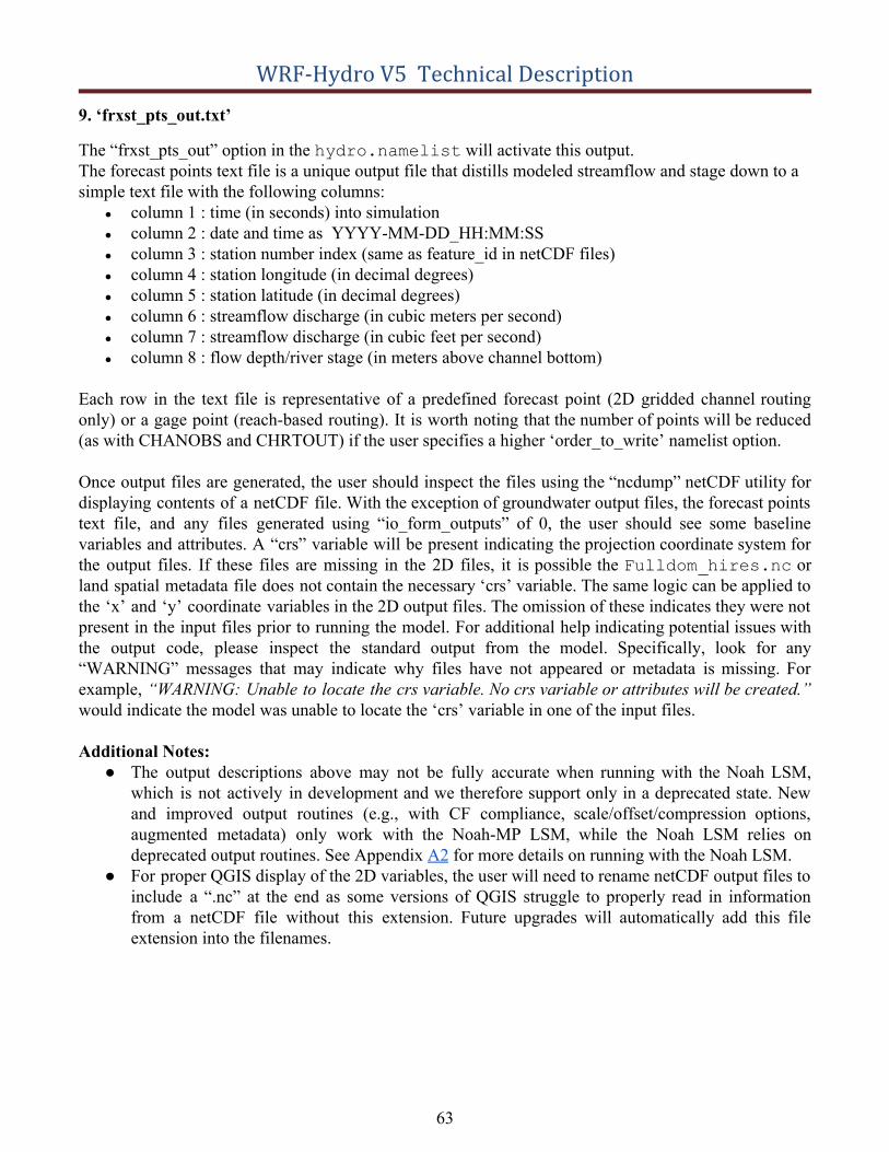
WRF-Hydro V5 Technical Description
9. ‘frxst_pts_out.txt’
The “frxst_pts_out” option in the hydro.namelist will activate this output.The forecast points text file is a unique output file that distills modeled streamflow and stage down to a simple text file with the following columns:
● column 1 : time (in seconds) into simulation● column 2 : date and time as YYYY-MM-DD_HH:MM:SS● column 3 : station number index (same as feature_id in netCDF files)● column 4 : station longitude (in decimal degrees)● column 5 : station latitude (in decimal degrees)● column 6 : streamflow discharge (in cubic meters per second)● column 7 : streamflow discharge (in cubic feet per second)● column 8 : flow depth/river stage (in meters above channel bottom)
Each row in the text file is representative of a predefined forecast point (2D gridded channel routing only) or a gage point (reach-based routing). It is worth noting that the number of points will be reduced (as with CHANOBS and CHRTOUT) if the user specifies a higher ‘order_to_write’ namelist option.
Once output files are generated, the user should inspect the files using the “ncdump” netCDF utility for displaying contents of a netCDF file. With the exception of groundwater output files, the forecast points text file, and any files generated using “io_form_outputs” of 0, the user should see some baseline variables and attributes. A “crs” variable will be present indicating the projection coordinate system for the output files. If these files are missing in the 2D files, it is possible the Fulldom_hires.nc or land spatial metadata file does not contain the necessary ‘crs’ variable. The same logic can be applied to the ‘x’ and ‘y’ coordinate variables in the 2D output files. The omission of these indicates they were not present in the input files prior to running the model. For additional help indicating potential issues with the output code, please inspect the standard output from the model. Specifically, look for any “WARNING” messages that may indicate why files have not appeared or metadata is missing. For example, “WARNING: Unable to locate the crs variable. No crs variable or attributes will be created.” would indicate the model was unable to locate the ‘crs’ variable in one of the input files.
Additional Notes: ● The output descriptions above may not be fully accurate when running with the Noah LSM,
which is not actively in development and we therefore support only in a deprecated state. New and improved output routines (e.g., with CF compliance, scale/offset/compression options, augmented metadata) only work with the Noah-MP LSM, while the Noah LSM relies on deprecated output routines. See Appendix A2 for more details on running with the Noah LSM.
● For proper QGIS display of the 2D variables, the user will need to rename netCDF output files to include a “.nc” at the end as some versions of QGIS struggle to properly read in information from a netCDF file without this extension. Future upgrades will automatically add this file extension into the filenames.
63
WRF-Hydro V5 Technical Description
REFERENCES Below are cited references in an alphabetical listing by author.
Ball, J. T., I. E. Woodrow, and J. A. Berry (1987), A model predicting stomatal conductance and its contribution to the control of photosynthesis under different environmental conditions, in Process in Photosynthesis Research, vol. 1, edited by J. Biggins, pp. 221–234, Martinus Nijhoff, Dordrecht, Netherlands.
Bowling, L.C., D.P. Lettenmaier, B. Nijssen, L.P. Graham and co-authors, 2003: Simulation of high latitude hydrological processes in the Torne-Kalix basin: PILPS Phase 2(c) 1: Experiment description and summary intercomparisons. Global and Planet. Change
Bryan, F. O., B. G. Kauffman, W. G. Large, and P. R. Gent (1996). The NCAR CSM flux coupler, NCAR Tech. Note 424, 50 pp. [Available from NCAR, Boulder, CO 80307]
Chen, F., K.E. Mitchell, J. Schaake, Y. Xue, H.-L. Pan, V. Koren, Q.Y. Duan, M. Ek and A. Betts, 1996: Modeling of land-surface evaporation by four schemes and comparison with FIFE observations. J. Geophys. Res., 101, 7251-7268.
Chen, F., Z. Janic and K.E. Mitchell, 1997: Impact of atmospheric surface-layer parameterizations in the new land-surface scheme of the NCEP mesoscale Eta model. Bound.-Layer Meteorol., 85, 391-421.
Chen, F. and K.E. Mitchell, 1999: Using the GEWEX/ISLSCP forcing data to simulate global soil moisture fields and hydrological cycle for 1987-1988, J. Meteorol. Soc. Japan, 77, 167-182.
Dickinson, R. E., M. Shaikh, R. Bryant, and L. Graumlich (1998), Interactive canopies for a climate model, J. Clim., 11, 2823–2836, doi:10.1175/1520-0442.
Dirmeyer, P.A., A.J. Dolman, N. Sato, 1999: The pilot phase of the Global Soil Wetness Project. Bull. Am. Meteorol. Soc., 80(5), 851-878.
Ek, M.B., K.E. Mitchell, Y. Lin, E. Rogers, P. Grunmann, V. Koren, G. Gayno, and J.D. Tarpley, 2003: Implementation of Noah land surface model advances in the NCEP operational mesoscale Eta model. Submitted to J. Geophys. Res., Aug., 2003.
Gochis, D.J. and F. Chen, 2003: Hydrological enhancements to the community Noah land surface model. NCAR Technical Note, NCAR/TN-454+STR, 68 pgs.
Jones, P. W. (1999). First- and Second-Order Conservative Remapping Schemes for Grids in Spherical Coordinates, Monthly Weather Review, Volume 127, 2204-2210.
Julien, P.Y., B. Saghafian and F.L. Ogden, 1995: Raster-based hydrological modeling of spatially-varied surface runoff. Water Resour. Bull., AWRA, 31(3), 523-536.
Koren, V., J.C. Schaake, K.E. Mitchell, Q.Y. Duan, F. Chen and J. Baker, 1999: A parameterization of snowpack and frozen ground intended for NCEP weather and climate models. J. Geophys. Res., 104(D16), 19,569-19,585.
LDAS, 2003: Land Data Assimilation Systems (LDAS). World Wide Web Homepage. Available online at: http://ldas.gsfc.nasa.gov/
64
WRF-Hydro V5 Technical Description
Mahrt, L. and H.-L. Pan, 1984: A two-layer model of soil hydrology. Bound.-Layer Meteorol., 29, 1-20, 1984.
Niu, G.-Y., et al. (2011), The community Noah land surface model with multiparameterization options (Noah-MP): 1. Model description and evaluation with local-scale measurements, J. Geophys. Res. 116, D12109, doi: 10.1029/2010JD015139.
Niu, G.-Y., and Z.-L. Yang (2004), The effects of canopy processes on snow surface energy and mass balances, J. Geophys. Res., 109, D23111, doi:10.1029/2004JD004884.
Niu, G.-Y., Z.-L. Yang, R. E. Dickinson, L. E. Gulden, and H. Su (2007), Development of a simple groundwater model for use in climate models and evaluation with Gravity Recovery and Climate Experiment data, J. Geophys. Res., 112, D07103, doi:10.1029/2006JD007522.
Ogden, F.L., 1997: CASC2D Reference Manual. Dept. of Civil and Evniron. Eng. U-37, U. Connecticut, 106 pp.
Pan, H.-L. and L. Mahrt, 1987: Interaction between soil hydrology and boundary-layer development, Bound.-Layer Meteorol., 38, 185-202.
Skamarock, W. C., J. B. Klemp, J. Dudhia, D. O. Gill, D. M. Barker, W. Wang, and J. G. Powers, 2005: A Description of the Advanced Research WRF Version 2. NCAR Technical Note NCAR/TN-468+STR, doi:10.5065/D6DZ069T.
Wigmosta, M.S. L.W. Vail and D.P. Lettenmaier, 1994: A distributed hydrology-vegetation model for complex terrain. Water Resour. Res., 30(6), 1665-1679.
Wigmosta, M.S. and D.P. Lettenmaier, 1999: A comparison of simplified methods for routing topographically driven subsurface flow. Water Resour. Res., 35(1), 255-264.
Wood, E.F., D.P. Lettenmaier, X. Kian, D. Lohmann, A. Boone, S. Chang, F.Chen, Y. Dai, R.E. Dickinson, Q. Duan, M. Ek, Y.M. Gusev, F. Habets, P. Irannejad, R. Koster, K.E. Mitchell, O.N. Nasonova, J. Noilhan, J. Schaake, A. Schlosser, Y. Shao, A.B. Shmakin, D. Verseghy, K. Warrach, P. Wetzel, Y. Xue, Z.-L. Yang, and Q.-C. Zeng, 1998: The project for intercomparison of land-surface parameterization schemes (PILPS) phase 2(c) Red-Arkansas river basin experiment: 1. Experiment description and summary intercomparisons, Global Planet. Change, 19, 115-135.
Yang, Z.-L., and G.-Y. Niu (2003), The versatile integrator of surface and atmosphere processes (VISA) part I: Model description, Global Planet. Change, 38, 175–189, doi:10.1016/S0921-8181(03)00028-6.
ESMF (Earth System Modeling Framework) https://www.earthsystemcog.org/projects/esmf/
USGS Global Land Cover Characterization https://www.usgs.gov/centers/eros/science/usgs-eros-archive-land-cover-products-global-land-cover-characterization-glcc-0?qt-science_center_objects=0#qt-science_center_objectsTable Legend: Appendix 3 https://edcftp.cr.usgs.gov/project/glcc/globdoc2_0.html#app3
IGBP_MODIS_BU+tundra Landcover Class Legend ftp://ftp.emc.ncep.noaa.gov/mmb/gcp/ldas/noahlsm/README NCL (NCAR Command Language) https://www.ncl.ucar.edu/ CDO (Climate Data Operators) https://code.mpimet.mpg.de/projects/cdo/
65
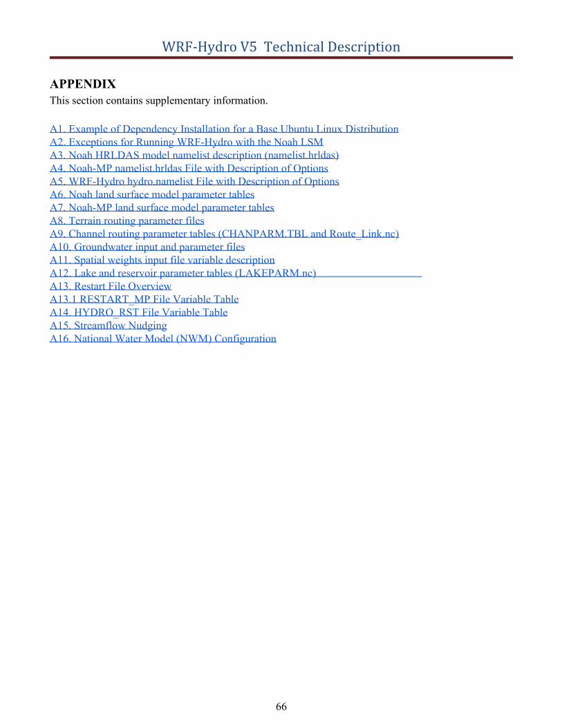
WRF-Hydro V5 Technical Description
APPENDIXThis section contains supplementary information.
A1. Example of Dependency Installation for a Base Ubuntu Linux Distribution A2. Exceptions for Running WRF-Hydro with the Noah LSM A3. Noah HRLDAS model namelist description (namelist.hrldas) A4. Noah-MP namelist.hrldas File with Description of Options A5. WRF-Hydro hydro.namelist File with Description of Options A6. Noah land surface model parameter tables A7. Noah-MP land surface model parameter tables A8. Terrain routing parameter files A9. Channel routing parameter tables (CHANPARM.TBL and Route_Link.nc) A10. Groundwater input and parameter files A11. Spatial weights input file variable description A12. Lake and reservoir parameter tables (LAKEPARM.nc) A13. Restart File Overview A13.1 RESTART_MP File Variable Table A14. HYDRO_RST File Variable Table A15. Streamflow Nudging A16. National Water Model (NWM) Configuration
66

WRF-Hydro V5 Technical Description
A1. Example of Dependency Installation for a Base Ubuntu Linux Distribution The example below uses the GNU compiler and MPICH libraries, and commands are issued as root user in the bash shell.
################################## ###Get libraries available through apt-get ################################## apt-get update
apt-get install -yq --no-install-recommends \
wget \
bzip2 \
ca-certificates \
libhdf5-dev \
gfortran \
m4 \
make \
libswitch-perl
apt-get clean
################################## ###Install MPICH ##################################
#Define variables used for retrieving and building MPICH MPICH_VERSION="3.2"
MPICH_CONFIGURE_OPTIONS="--disable-cxx"
MPICH_MAKE_OPTIONS=''
#Make a temp directory for the MPICH source code mkdir /tmp/mpich-src
cd /tmp/mpich-src
#Download MPICH source code for specified version wget http://www.mpich.org/static/downloads/${MPICH_VERSION}/mpich-${MPICH_VERSION}.tar.gz
tar xfz mpich-${MPICH_VERSION}.tar.gz
cd mpich-${MPICH_VERSION}
#Configure and build MPICH ./configure ${MPICH_CONFIGURE_OPTIONS}
make ${MPICH_MAKE_OPTIONS}
make install
rm -rf /tmp/mpich-src
################################## ###Install NETCDF-C (>=4.0) ##################################
#Define variables used for retrieving and building HDF5 and NETCDF export H5DIR=/usr/lib/x86_64-linux-gnu/hdf5/serial export NCDIR=/usr/local NETCDF_C_VERSION="4.4.1.1"
#Download the NETCDF source code for specified version wget ftp://ftp.unidata.ucar.edu/pub/netcdf/netcdf-${NETCDF_C_VERSION}.tar.gz -P /tmp
67
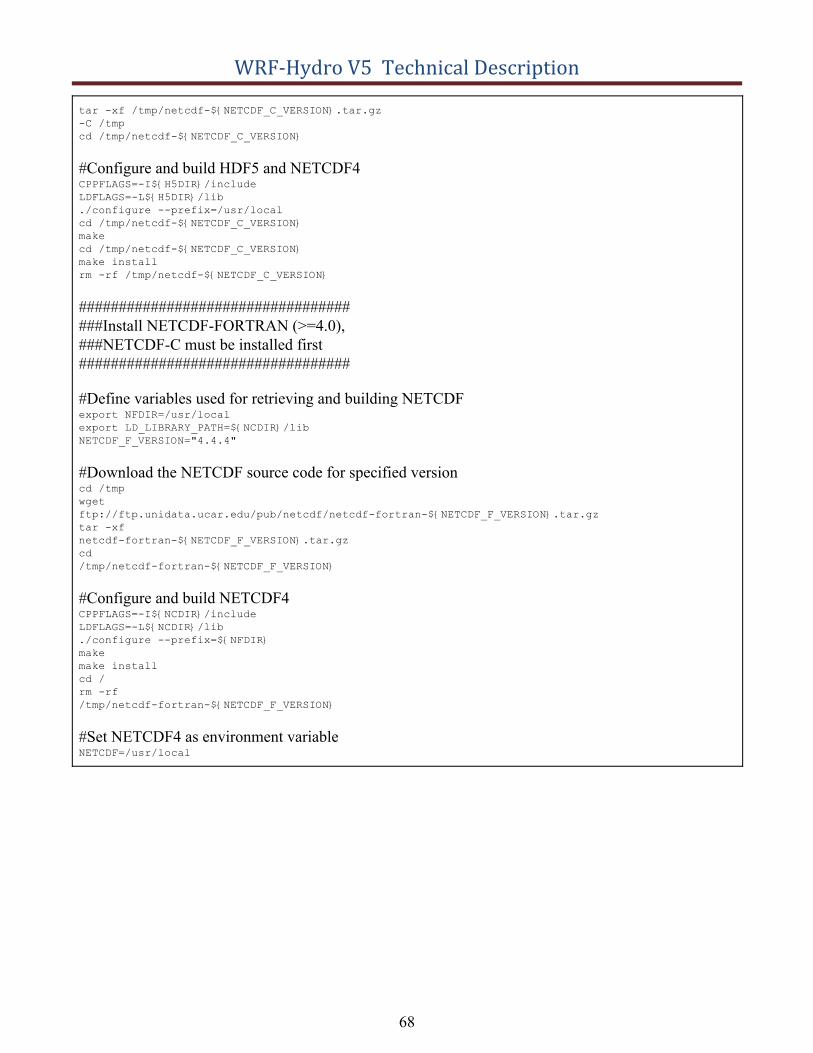
WRF-Hydro V5 Technical Description
tar -xf /tmp/netcdf-${NETCDF_C_VERSION}.tar.gz
-C /tmp
cd /tmp/netcdf-${NETCDF_C_VERSION}
#Configure and build HDF5 and NETCDF4 CPPFLAGS=-I${H5DIR}/include
LDFLAGS=-L${H5DIR}/lib
./configure --prefix=/usr/local
cd /tmp/netcdf-${NETCDF_C_VERSION}
make
cd /tmp/netcdf-${NETCDF_C_VERSION}
make install
rm -rf /tmp/netcdf-${NETCDF_C_VERSION}
################################## ###Install NETCDF-FORTRAN (>=4.0), ###NETCDF-C must be installed first ##################################
#Define variables used for retrieving and building NETCDF export NFDIR=/usr/local
export LD_LIBRARY_PATH=${NCDIR}/lib
NETCDF_F_VERSION="4.4.4"
#Download the NETCDF source code for specified version cd /tmp
wget
ftp://ftp.unidata.ucar.edu/pub/netcdf/netcdf-fortran-${NETCDF_F_VERSION}.tar.gz
tar -xf
netcdf-fortran-${NETCDF_F_VERSION}.tar.gz
cd
/tmp/netcdf-fortran-${NETCDF_F_VERSION}
#Configure and build NETCDF4 CPPFLAGS=-I${NCDIR}/include
LDFLAGS=-L${NCDIR}/lib
./configure --prefix=${NFDIR}
make
make install
cd /
rm -rf
/tmp/netcdf-fortran-${NETCDF_F_VERSION}
#Set NETCDF4 as environment variable NETCDF=/usr/local
68
WRF-Hydro V5 Technical Description
A2. Exceptions for Running WRF-Hydro with the Noah LSM Support for the Noah Land Surface Model (LSM) within WRF-Hydro is currently frozen at Noah version 3.6. Since the Noah LSM is not under active development by the community, WRF-Hydro is continuing to support Noah in deprecated mode only. Some new model features, such as the improved output routines, have not been setup to be backward compatible with Noah. Noah users should follow the guidelines below for adapting the WRF-Hydro workflow to work with Noah:
● LSM initialization: The simple wrfinput.nc initialization file created by thecreate_Wrfinput.R script does not currently include all of the fields required by the NoahLSM. Therefore, Noah users should use the WRF real.exe utility to create awrfinput_d0x file. Refer to the WRF documentation and user guides for information on howto do this.
● Time-varying vegetation specifications: While the Noah LSM will be properly initialized withgreen vegetation fraction from the wrfinput file, there is currently no automated method toupdate this field over time (e.g., seasonally based on climatology). Therefore, Noah users willneed to provide these time-varying fields in the model input forcing files (e.g., LDASIN).
● Spatially varying parameters : Spatially varying soil and vegetation parameters (e.g.,soil_properties.nc) are not supported in Noah.
● Model outputs: The updated output routines have not been adapted to work with Noah.Therefore, Noah users should always use io_form_outputs = 0 to activate the deprecated outputroutines. Scale/offset and compression options, CF compliance, augmented spatial metadata, etc.are not available in this deprecated mode.
69
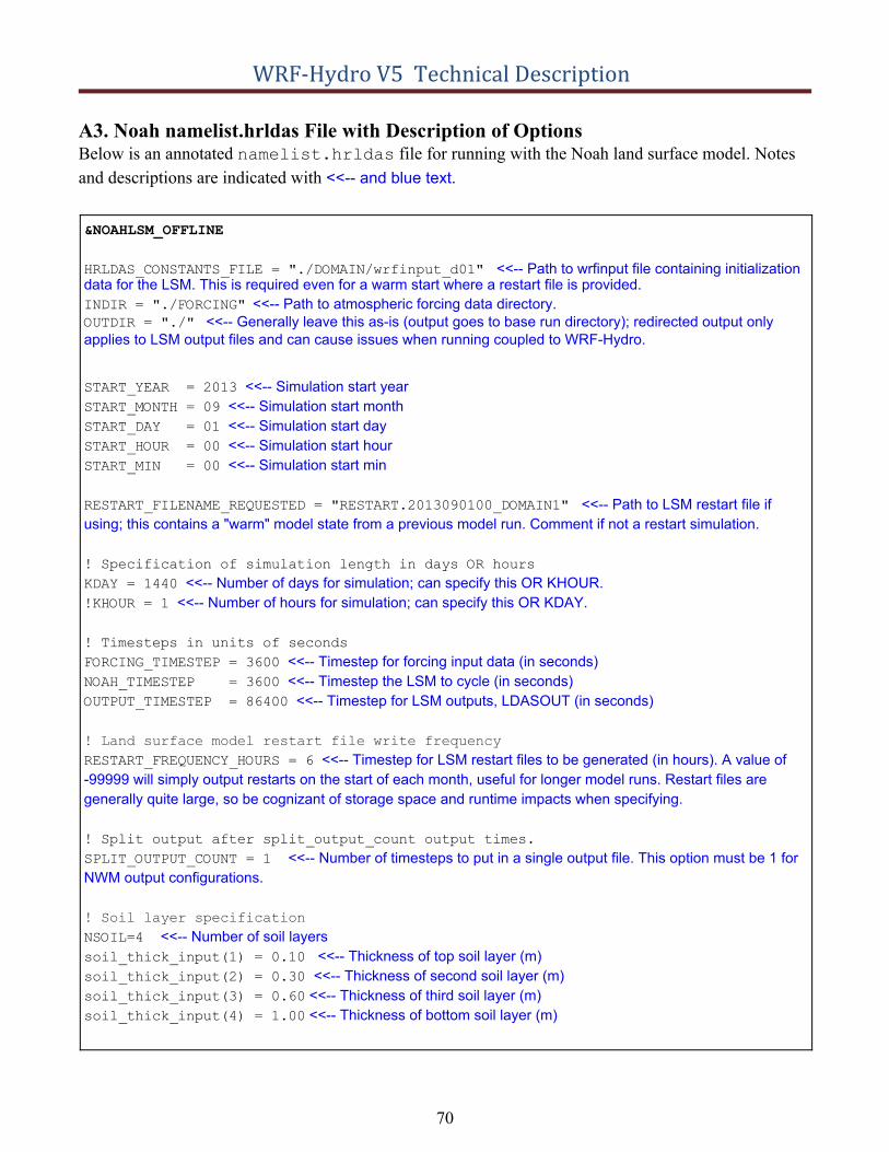
WRF-Hydro V5 Technical Description
A3. Noah namelist.hrldas File with Description of Options Below is an annotated namelist.hrldas file for running with the Noah land surface model. Notesand descriptions are indicated with <<-- and blue text.
&NOAHLSM_OFFLINE
HRLDAS_CONSTANTS_FILE = "./DOMAIN/wrfinput_d01" <<-- Path to wrfinput file containing initializationdata for the LSM. This is required even for a warm start where a restart file is provided. INDIR = "./FORCING" <<-- Path to atmospheric forcing data directory.OUTDIR = "./" <<-- Generally leave this as-is (output goes to base run directory); redirected output onlyapplies to LSM output files and can cause issues when running coupled to WRF-Hydro.
START_YEAR = 2013 <<-- Simulation start yearSTART_MONTH = 09 <<-- Simulation start month START_DAY = 01 <<-- Simulation start daySTART_HOUR = 00 <<-- Simulation start hour START_MIN = 00 <<-- Simulation start min
RESTART_FILENAME_REQUESTED = "RESTART.2013090100_DOMAIN1" <<-- Path to LSM restart file ifusing; this contains a "warm" model state from a previous model run. Comment if not a restart simulation.
! Specification of simulation length in days OR hours
KDAY = 1440 <<-- Number of days for simulation; can specify this OR KHOUR.!KHOUR = 1 <<-- Number of hours for simulation; can specify this OR KDAY.
! Timesteps in units of seconds
FORCING_TIMESTEP = 3600 <<-- Timestep for forcing input data (in seconds)NOAH_TIMESTEP = 3600 <<-- Timestep the LSM to cycle (in seconds)OUTPUT_TIMESTEP = 86400 <<-- Timestep for LSM outputs, LDASOUT (in seconds)
! Land surface model restart file write frequency
RESTART_FREQUENCY_HOURS = 6 <<-- Timestep for LSM restart files to be generated (in hours). A value of-99999 will simply output restarts on the start of each month, useful for longer model runs. Restart files aregenerally quite large, so be cognizant of storage space and runtime impacts when specifying.
! Split output after split_output_count output times.
SPLIT_OUTPUT_COUNT = 1 <<-- Number of timesteps to put in a single output file. This option must be 1 forNWM output configurations.
! Soil layer specification
NSOIL=4 <<-- Number of soil layerssoil_thick_input(1) = 0.10 <<-- Thickness of top soil layer (m)soil_thick_input(2) = 0.30 <<-- Thickness of second soil layer (m)soil_thick_input(3) = 0.60 <<-- Thickness of third soil layer (m)soil_thick_input(4) = 1.00 <<-- Thickness of bottom soil layer (m)
70
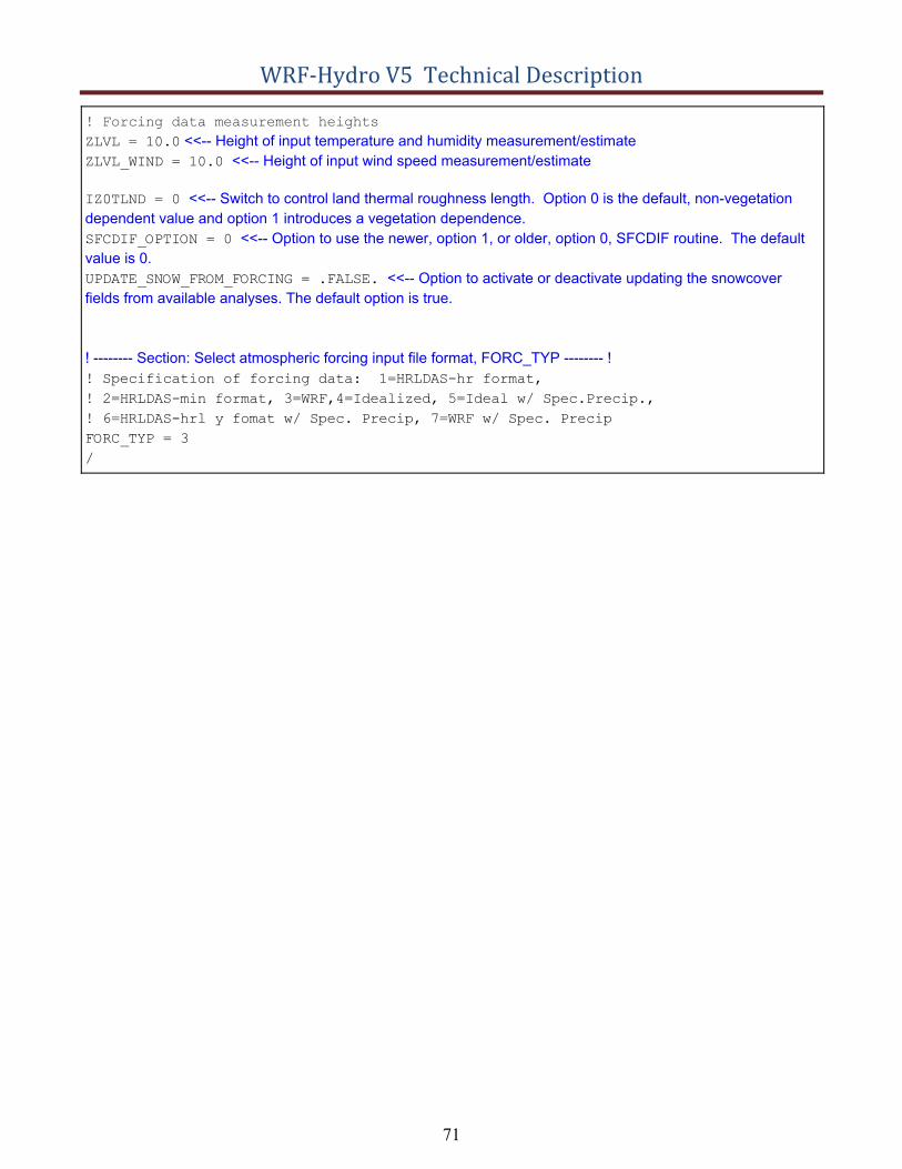
WRF-Hydro V5 Technical Description
! Forcing data measurement heights
ZLVL = 10.0 <<-- Height of input temperature and humidity measurement/estimateZLVL_WIND = 10.0 <<-- Height of input wind speed measurement/estimate
IZ0TLND = 0 <<-- Switch to control land thermal roughness length. Option 0 is the default, non-vegetationdependent value and option 1 introduces a vegetation dependence. SFCDIF_OPTION = 0 <<-- Option to use the newer, option 1, or older, option 0, SFCDIF routine. The defaultvalue is 0. UPDATE_SNOW_FROM_FORCING = .FALSE. <<-- Option to activate or deactivate updating the snowcoverfields from available analyses. The default option is true.
! -------- Section: Select atmospheric forcing input file format, FORC_TYP -------- !! Specification of forcing data: 1=HRLDAS-hr format,
! 2=HRLDAS-min format, 3=WRF,4=Idealized, 5=Ideal w/ Spec.Precip.,
! 6=HRLDAS-hrl y fomat w/ Spec. Precip, 7=WRF w/ Spec. Precip
FORC_TYP = 3
/
71
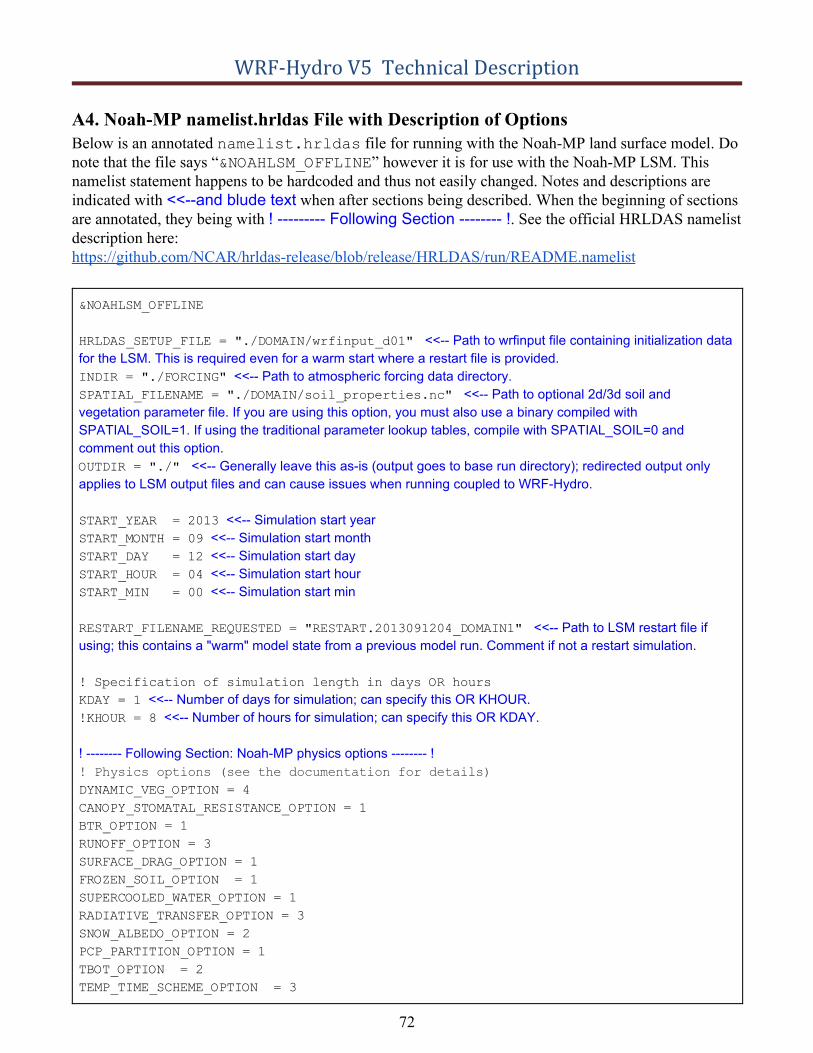
WRF-Hydro V5 Technical Description
A4. Noah-MP namelist.hrldas File with Description of Options Below is an annotated namelist.hrldas file for running with the Noah-MP land surface model. Donote that the file says “&NOAHLSM_OFFLINE” however it is for use with the Noah-MP LSM. Thisnamelist statement happens to be hardcoded and thus not easily changed. Notes and descriptions are indicated with <<--and blude text when after sections being described. When the beginning of sections are annotated, they being with ! --------- Following Section -------- !. See the official HRLDAS namelist description here: https://github.com/NCAR/hrldas-release/blob/release/HRLDAS/run/README.namelist
&NOAHLSM_OFFLINE
HRLDAS_SETUP_FILE = "./DOMAIN/wrfinput_d01" <<-- Path to wrfinput file containing initialization datafor the LSM. This is required even for a warm start where a restart file is provided. INDIR = "./FORCING" <<-- Path to atmospheric forcing data directory.SPATIAL_FILENAME = "./DOMAIN/soil_properties.nc" <<-- Path to optional 2d/3d soil andvegetation parameter file. If you are using this option, you must also use a binary compiled with SPATIAL_SOIL=1. If using the traditional parameter lookup tables, compile with SPATIAL_SOIL=0 and comment out this option. OUTDIR = "./" <<-- Generally leave this as-is (output goes to base run directory); redirected output onlyapplies to LSM output files and can cause issues when running coupled to WRF-Hydro.
START_YEAR = 2013 <<-- Simulation start yearSTART_MONTH = 09 <<-- Simulation start month START_DAY = 12 <<-- Simulation start daySTART_HOUR = 04 <<-- Simulation start hour START_MIN = 00 <<-- Simulation start min
RESTART_FILENAME_REQUESTED = "RESTART.2013091204_DOMAIN1" <<-- Path to LSM restart file ifusing; this contains a "warm" model state from a previous model run. Comment if not a restart simulation.
! Specification of simulation length in days OR hours
KDAY = 1 <<-- Number of days for simulation; can specify this OR KHOUR.!KHOUR = 8 <<-- Number of hours for simulation; can specify this OR KDAY.
! -------- Following Section: Noah-MP physics options -------- !! Physics options (see the documentation for details)
DYNAMIC_VEG_OPTION = 4
CANOPY_STOMATAL_RESISTANCE_OPTION = 1
BTR_OPTION = 1
RUNOFF_OPTION = 3
SURFACE_DRAG_OPTION = 1
FROZEN_SOIL_OPTION = 1
SUPERCOOLED_WATER_OPTION = 1
RADIATIVE_TRANSFER_OPTION = 3
SNOW_ALBEDO_OPTION = 2
PCP_PARTITION_OPTION = 1
TBOT_OPTION = 2
TEMP_TIME_SCHEME_OPTION = 3
72
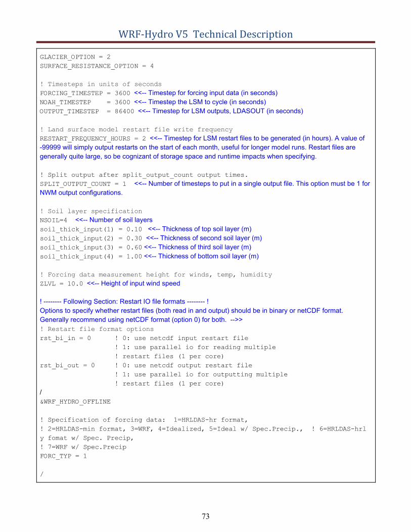
WRF-Hydro V5 Technical Description
GLACIER_OPTION = 2
SURFACE_RESISTANCE_OPTION = 4
! Timesteps in units of seconds
FORCING_TIMESTEP = 3600 <<-- Timestep for forcing input data (in seconds)NOAH_TIMESTEP = 3600 <<-- Timestep the LSM to cycle (in seconds)OUTPUT_TIMESTEP = 86400 <<-- Timestep for LSM outputs, LDASOUT (in seconds)
! Land surface model restart file write frequency
RESTART_FREQUENCY_HOURS = 2 <<-- Timestep for LSM restart files to be generated (in hours). A value of-99999 will simply output restarts on the start of each month, useful for longer model runs. Restart files aregenerally quite large, so be cognizant of storage space and runtime impacts when specifying.
! Split output after split_output_count output times.
SPLIT_OUTPUT_COUNT = 1 <<-- Number of timesteps to put in a single output file. This option must be 1 forNWM output configurations.
! Soil layer specification
NSOIL=4 <<-- Number of soil layerssoil_thick_input(1) = 0.10 <<-- Thickness of top soil layer (m)soil_thick_input(2) = 0.30 <<-- Thickness of second soil layer (m)soil_thick_input(3) = 0.60 <<-- Thickness of third soil layer (m)soil_thick_input(4) = 1.00 <<-- Thickness of bottom soil layer (m)
! Forcing data measurement height for winds, temp, humidity
ZLVL = 10.0 <<-- Height of input wind speed
! -------- Following Section: Restart IO file formats -------- !Options to specify whether restart files (both read in and output) should be in binary or netCDF format.Generally recommend using netCDF format (option 0) for both. -->>! Restart file format options
rst_bi_in = 0 ! 0: use netcdf input restart file
! 1: use parallel io for reading multiple
! restart files (1 per core)
rst_bi_out = 0 ! 0: use netcdf output restart file
! 1: use parallel io for outputting multiple
! restart files (1 per core)
/ &WRF_HYDRO_OFFLINE
! Specification of forcing data: 1=HRLDAS-hr format,
! 2=HRLDAS-min format, 3=WRF, 4=Idealized, 5=Ideal w/ Spec.Precip., ! 6=HRLDAS-hrl
y fomat w/ Spec. Precip,
! 7=WRF w/ Spec.Precip
FORC_TYP = 1
/
73
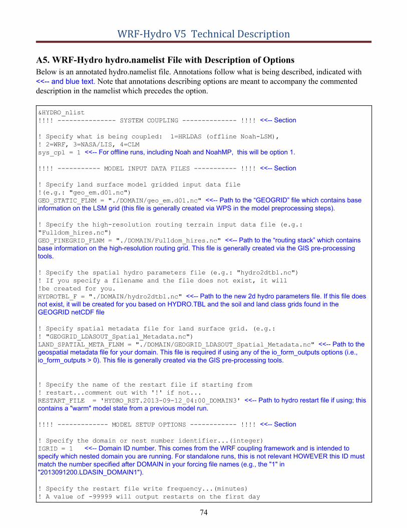
WRF-Hydro V5 Technical Description
A5. WRF-Hydro hydro.namelist File with Description of Options Below is an annotated hydro.namelist file. Annotations follow what is being described, indicated with <<-- and blue text. Note that annotations describing options are meant to accompany the commented description in the namelist which precedes the option.
&HYDRO_nlist
!!!! --------------- SYSTEM COUPLING -------------- !!!! <<-- Section
! Specify what is being coupled: 1=HRLDAS (offline Noah-LSM),
! 2=WRF, 3=NASA/LIS, 4=CLM
sys_cpl = 1 <<-- For offline runs, including Noah and NoahMP, this will be option 1.
!!!! ----------- MODEL INPUT DATA FILES ----------- !!!! <<-- Section
! Specify land surface model gridded input data file
!(e.g.: "geo_em.d01.nc")
GEO_STATIC_FLNM = "./DOMAIN/geo_em.d01.nc" <<-- Path to the “GEOGRID” file which contains baseinformation on the LSM grid (this file is generally created via WPS in the model preprocessing steps).
! Specify the high-resolution routing terrain input data file (e.g.:
"Fulldom_hires.nc")
GEO_FINEGRID_FLNM = "./DOMAIN/Fulldom_hires.nc" <<-- Path to the “routing stack” which containsbase information on the high-resolution routing grid. This file is generally created via the GIS pre-processingtools.
! Specify the spatial hydro parameters file (e.g.: "hydro2dtbl.nc")
! If you specify a filename and the file does not exist, it will
!be created for you.
HYDROTBL_F = "./DOMAIN/hydro2dtbl.nc" <<-- Path to the new 2d hydro parameters file. If this file doesnot exist, it will be created for you based on HYDRO.TBL and the soil and land class grids found in theGEOGRID netCDF file
! Specify spatial metadata file for land surface grid. (e.g.:
! "GEOGRID_LDASOUT_Spatial_Metadata.nc")
LAND_SPATIAL_META_FLNM = "./DOMAIN/GEOGRID_LDASOUT_Spatial_Metadata.nc" <<-- Path to thegeospatial metadata file for your domain. This file is required if using any of the io_form_outputs options (i.e.,io_form_outputs > 0). This file is generally created via the GIS pre-processing tools.
! Specify the name of the restart file if starting from
! restart...comment out with '!' if not...
RESTART_FILE = 'HYDRO_RST.2013-09-12_04:00_DOMAIN3' <<-- Path to hydro restart file if using; thiscontains a "warm" model state from a previous model run.
!!!! ------------- MODEL SETUP OPTIONS ------------ !!!! <<-- Section
! Specify the domain or nest number identifier...(integer)
IGRID = 1 <<-- Domain ID number. This comes from the WRF coupling framework and is intended tospecify which nested domain you are running. For standalone runs, this is not relevant HOWEVER this ID mustmatch the number specified after DOMAIN in your forcing file names (e.g., the "1" in"2013091200.LDASIN_DOMAIN1").
! Specify the restart file write frequency...(minutes)
! A value of -99999 will output restarts on the first day
74
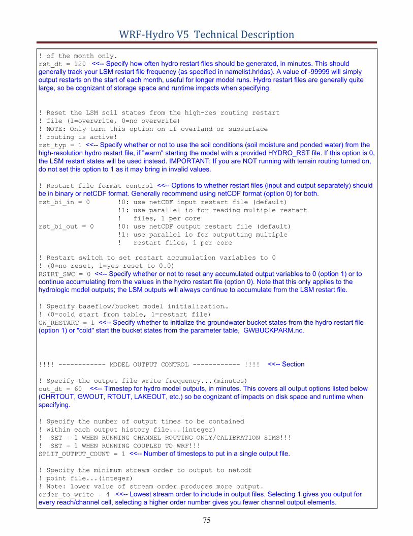
WRF-Hydro V5 Technical Description
! of the month only.
rst_dt = 120 <<-- Specify how often hydro restart files should be generated, in minutes. This shouldgenerally track your LSM restart file frequency (as specified in namelist.hrldas). A value of -99999 will simplyoutput restarts on the start of each month, useful for longer model runs. Hydro restart files are generally quitelarge, so be cognizant of storage space and runtime impacts when specifying.
! Reset the LSM soil states from the high-res routing restart
! file (1=overwrite, 0=no overwrite)
! NOTE: Only turn this option on if overland or subsurface
! routing is active!
rst_typ = 1 <<-- Specify whether or not to use the soil conditions (soil moisture and ponded water) from thehigh-resolution hydro restart file, if "warm" starting the model with a provided HYDRO_RST file. If this option is 0,the LSM restart states will be used instead. IMPORTANT: If you are NOT running with terrain routing turned on,do not set this option to 1 as it may bring in invalid values.
! Restart file format control <<-- Options to whether restart files (input and output separately) shouldbe in binary or netCDF format. Generally recommend using netCDF format (option 0) for both.rst_bi_in = 0 !0: use netCDF input restart file (default)
!1: use parallel io for reading multiple restart
! files, 1 per core
rst_bi_out = 0 !0: use netCDF output restart file (default)
!1: use parallel io for outputting multiple
! restart files, 1 per core
! Restart switch to set restart accumulation variables to 0
! (0=no reset, 1=yes reset to 0.0)
RSTRT_SWC = 0 <<-- Specify whether or not to reset any accumulated output variables to 0 (option 1) or tocontinue accumulating from the values in the hydro restart file (option 0). Note that this only applies to the hydrologic model outputs; the LSM outputs will always continue to accumulate from the LSM restart file.
! Specify baseflow/bucket model initialization…
! (0=cold start from table, 1=restart file)
GW_RESTART = 1 <<-- Specify whether to initialize the groundwater bucket states from the hydro restart file(option 1) or "cold" start the bucket states from the parameter table, GWBUCKPARM.nc.
!!!! ------------ MODEL OUTPUT CONTROL ------------ !!!! <<-- Section
! Specify the output file write frequency...(minutes)
out_dt = 60 <<-- Timestep for hydro model outputs, in minutes. This covers all output options listed below(CHRTOUT, GWOUT, RTOUT, LAKEOUT, etc.) so be cognizant of impacts on disk space and runtime whenspecifying.
! Specify the number of output times to be contained
! within each output history file...(integer)
! SET = 1 WHEN RUNNING CHANNEL ROUTING ONLY/CALIBRATION SIMS!!!
! SET = 1 WHEN RUNNING COUPLED TO WRF!!!
SPLIT_OUTPUT_COUNT = 1 <<-- Number of timesteps to put in a single output file.
! Specify the minimum stream order to output to netcdf
! point file...(integer)
! Note: lower value of stream order produces more output.
order_to_write = 4 <<-- Lowest stream order to include in output files. Selecting 1 gives you output forevery reach/channel cell, selecting a higher order number gives you fewer channel output elements.
75
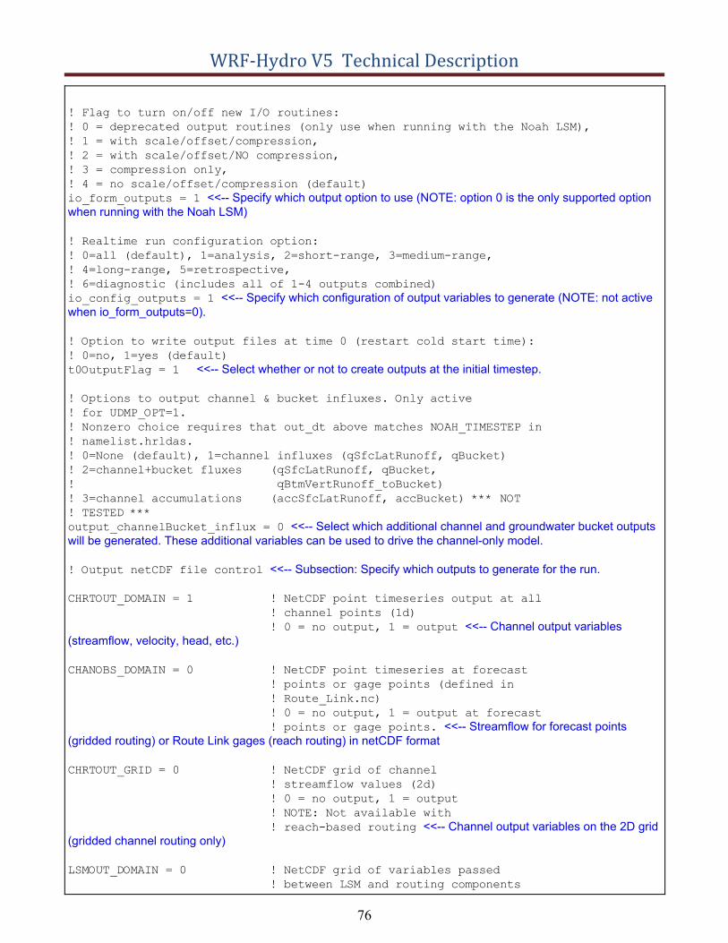
WRF-Hydro V5 Technical Description
! Flag to turn on/off new I/O routines:
! 0 = deprecated output routines (only use when running with the Noah LSM),
! 1 = with scale/offset/compression,
! 2 = with scale/offset/NO compression,
! 3 = compression only,
! 4 = no scale/offset/compression (default)
io_form_outputs = 1 <<-- Specify which output option to use (NOTE: option 0 is the only supported optionwhen running with the Noah LSM)
! Realtime run configuration option:
! 0=all (default), 1=analysis, 2=short-range, 3=medium-range,
! 4=long-range, 5=retrospective,
! 6=diagnostic (includes all of 1-4 outputs combined)
io_config_outputs = 1 <<-- Specify which configuration of output variables to generate (NOTE: not activewhen io_form_outputs=0).
! Option to write output files at time 0 (restart cold start time):
! 0=no, 1=yes (default)
t0OutputFlag = 1 <<-- Select whether or not to create outputs at the initial timestep.
! Options to output channel & bucket influxes. Only active
! for UDMP_OPT=1.
! Nonzero choice requires that out_dt above matches NOAH_TIMESTEP in
! namelist.hrldas.
! 0=None (default), 1=channel influxes (qSfcLatRunoff, qBucket)
! 2=channel+bucket fluxes (qSfcLatRunoff, qBucket,
! qBtmVertRunoff_toBucket)
! 3=channel accumulations (accSfcLatRunoff, accBucket) *** NOT
! TESTED ***
output_channelBucket_influx = 0 <<-- Select which additional channel and groundwater bucket outputswill be generated. These additional variables can be used to drive the channel-only model.
! Output netCDF file control <<-- Subsection: Specify which outputs to generate for the run.
CHRTOUT_DOMAIN = 1 ! NetCDF point timeseries output at all
! channel points (1d)
! 0 = no output, 1 = output <<-- Channel output variables(streamflow, velocity, head, etc.)
CHANOBS_DOMAIN = 0 ! NetCDF point timeseries at forecast
! points or gage points (defined in
! Route_Link.nc)
! 0 = no output, 1 = output at forecast
! points or gage points. <<-- Streamflow for forecast points(gridded routing) or Route Link gages (reach routing) in netCDF format
CHRTOUT_GRID = 0 ! NetCDF grid of channel
! streamflow values (2d)
! 0 = no output, 1 = output
! NOTE: Not available with
! reach-based routing <<-- Channel output variables on the 2D grid(gridded channel routing only)
LSMOUT_DOMAIN = 0 ! NetCDF grid of variables passed
! between LSM and routing components
76
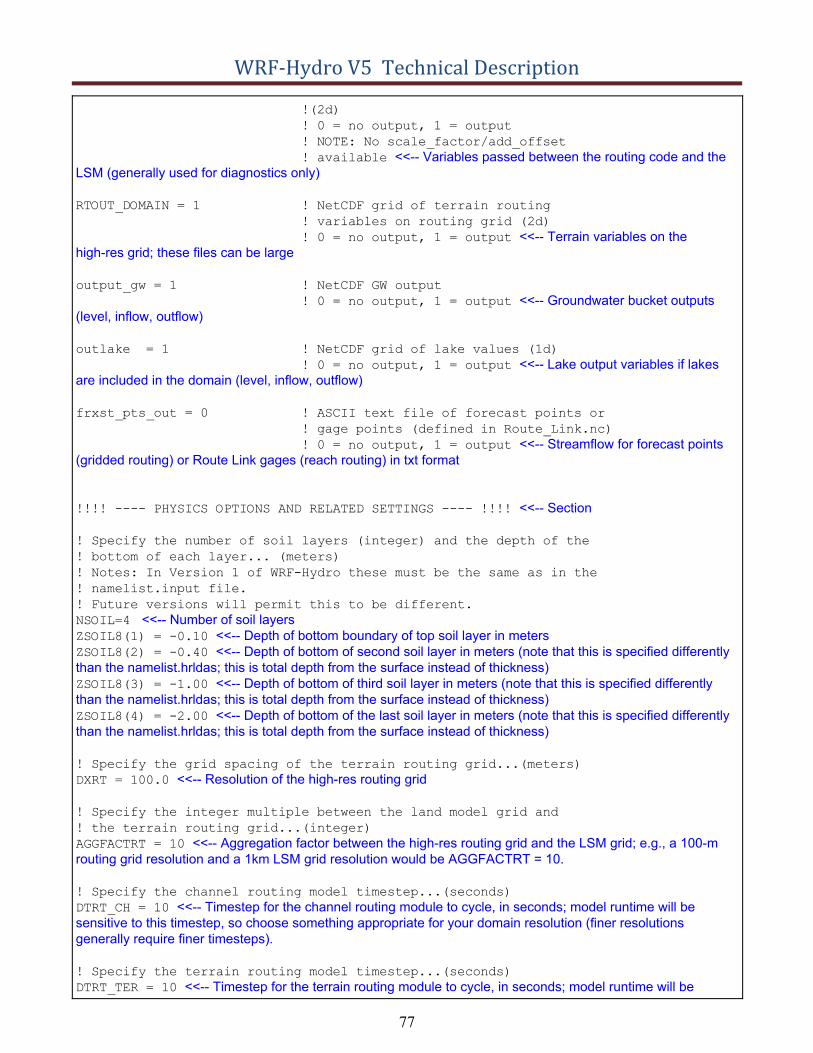
WRF-Hydro V5 Technical Description
!(2d)
! 0 = no output, 1 = output
! NOTE: No scale_factor/add_offset
! available <<-- Variables passed between the routing code and theLSM (generally used for diagnostics only)
RTOUT_DOMAIN = 1 ! NetCDF grid of terrain routing
! variables on routing grid (2d)
! 0 = no output, 1 = output <<-- Terrain variables on thehigh-res grid; these files can be large
output_gw = 1 ! NetCDF GW output
! 0 = no output, 1 = output <<-- Groundwater bucket outputs(level, inflow, outflow)
outlake = 1 ! NetCDF grid of lake values (1d)
! 0 = no output, 1 = output <<-- Lake output variables if lakesare included in the domain (level, inflow, outflow)
frxst_pts_out = 0 ! ASCII text file of forecast points or
! gage points (defined in Route_Link.nc)
! 0 = no output, 1 = output <<-- Streamflow for forecast points(gridded routing) or Route Link gages (reach routing) in txt format
!!!! ---- PHYSICS OPTIONS AND RELATED SETTINGS ---- !!!! <<-- Section
! Specify the number of soil layers (integer) and the depth of the
! bottom of each layer... (meters)
! Notes: In Version 1 of WRF-Hydro these must be the same as in the
! namelist.input file.
! Future versions will permit this to be different.
NSOIL=4 <<-- Number of soil layersZSOIL8(1) = -0.10 <<-- Depth of bottom boundary of top soil layer in metersZSOIL8(2) = -0.40 <<-- Depth of bottom of second soil layer in meters (note that this is specified differentlythan the namelist.hrldas; this is total depth from the surface instead of thickness)ZSOIL8(3) = -1.00 <<-- Depth of bottom of third soil layer in meters (note that this is specified differentlythan the namelist.hrldas; this is total depth from the surface instead of thickness) ZSOIL8(4) = -2.00 <<-- Depth of bottom of the last soil layer in meters (note that this is specified differentlythan the namelist.hrldas; this is total depth from the surface instead of thickness)
! Specify the grid spacing of the terrain routing grid...(meters)
DXRT = 100.0 <<-- Resolution of the high-res routing grid
! Specify the integer multiple between the land model grid and
! the terrain routing grid...(integer)
AGGFACTRT = 10 <<-- Aggregation factor between the high-res routing grid and the LSM grid; e.g., a 100-mrouting grid resolution and a 1km LSM grid resolution would be AGGFACTRT = 10.
! Specify the channel routing model timestep...(seconds)
DTRT_CH = 10 <<-- Timestep for the channel routing module to cycle, in seconds; model runtime will besensitive to this timestep, so choose something appropriate for your domain resolution (finer resolutionsgenerally require finer timesteps).
! Specify the terrain routing model timestep...(seconds)
DTRT_TER = 10 <<-- Timestep for the terrain routing module to cycle, in seconds; model runtime will be
77
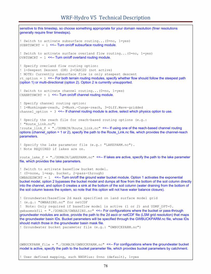
WRF-Hydro V5 Technical Description
sensitive to this timestep, so choose something appropriate for your domain resolution (finer resolutions generally require finer timesteps).
! Switch to activate subsurface routing...(0=no, 1=yes)
SUBRTSWCRT = 1 <<-- Turn on/off subsurface routing module.
! Switch to activate surface overland flow routing...(0=no, 1=yes)
OVRTSWCRT = 1 <<-- Turn on/off overland routing module.
! Specify overland flow routing option:
! 1=Seepest Descent (D8) 2=CASC2D (not active)
! NOTE: Currently subsurface flow is only steepest descent
rt_option = 1 <<-- For both terrain routing modules, specify whether flow should follow the steepest path(option 1) or multi-directional (option 2). Option 2 is currently unsupported.
! Switch to activate channel routing...(0=no, 1=yes)
CHANRTSWCRT = 1 <<-- Turn on/off channel routing module.
! Specify channel routing option:
! 1=Muskingam-reach, 2=Musk.-Cunge-reach, 3=Diff.Wave-gridded
channel_option = 3 <<-- If channel routing module is active, select which physics option to use.
! Specify the reach file for reach-based routing options (e.g.:
! "Route_Link.nc")
!route_link_f = "./DOMAIN/Route_Link.nc" <<-- If using one of the reach-based channel routingoptions (channel_option = 1 or 2), specify the path to the Route_Link.nc file, which provides the channel-reachparameters.
! Specify the lake parameter file (e.g.: "LAKEPARM.nc").
! Note REQUIRED if lakes are on.
route_lake_f = "./DOMAIN/LAKEPARM.nc" <<-- If lakes are active, specify the path to the lake parameterfile, which provides the lake parameters.
! Switch to activate baseflow bucket model…
! (0=none, 1=exp. bucket, 2=pass-through)
GWBASESWCRT = 1 <<-- Turn on/off the ground water bucket module. Option 1 activates the exponentialbucket model, option 2 bypasses the bucket model and dumps all flow from the bottom of the soil column directly into the channel, and option 0 creates a sink at the bottom of the soil column (water draining from the bottom of the soil column leaves the system, so note that this option will not have water balance closure).
! Groundwater/baseflow 2d mask specified on land surface model grid
! (e.g.: "GWBASINS.nc" for netCDF
! Note: Only required if baseflow model is active (1 or 2) and UDMP_OPT=0.gwbasmskfil = "./DOMAIN/GWBASINS.nc" <<-- For configurations where the bucket or pass-throughgroundwater modules are active, provide the path to the 2d ascii or netCDF file (LSM grid resolution) that maps the groundwater basin IDs. Bucket parameters will be specified through the GWBUCKPARM.nc file, whose IDs should match those in the groundwater basin mask file.! Groundwater bucket parameter file (e.g.: "GWBUCKPARM.nc")
GWBUCKPARM_file = "./DOMAIN/GWBUCKPARM.nc" <<-- For configurations where the groundwater bucketmodel is active, specify the path to the bucket parameter file, which provides bucket parameters by catchment.
! User defined mapping, such NHDPlus: 0=no (default), 1=yes
78
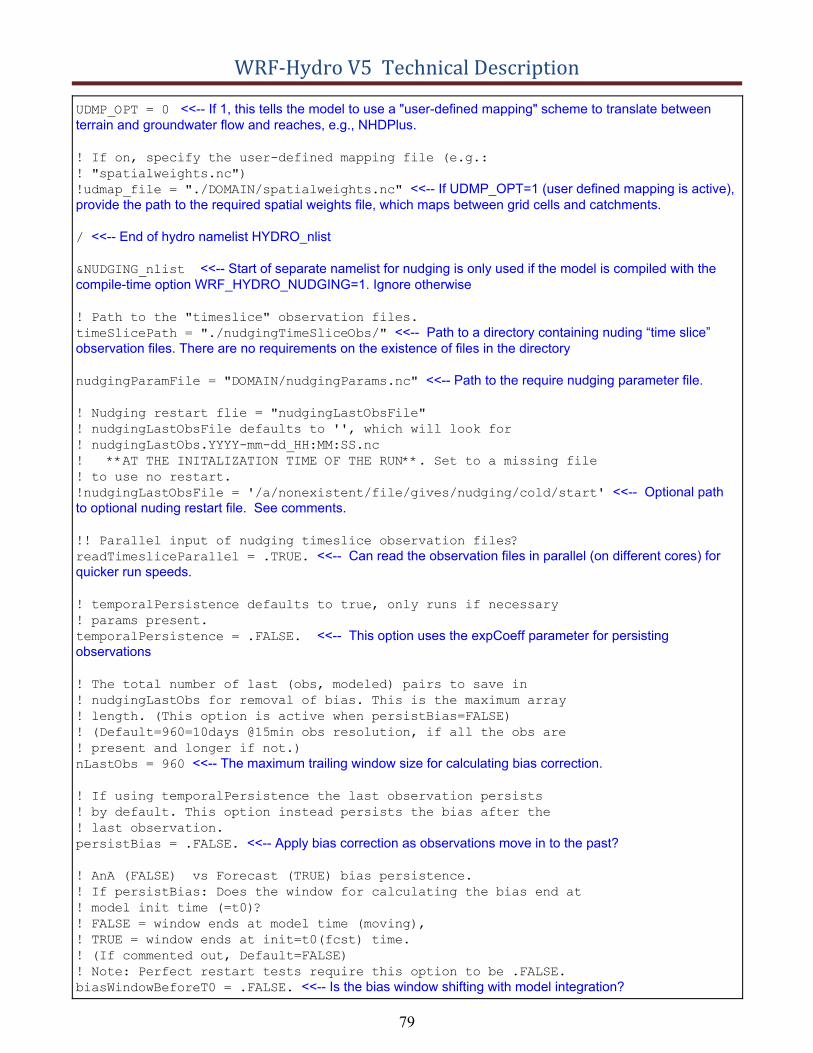
WRF-Hydro V5 Technical Description
UDMP_OPT = 0 <<-- If 1, this tells the model to use a "user-defined mapping" scheme to translate betweenterrain and groundwater flow and reaches, e.g., NHDPlus.
! If on, specify the user-defined mapping file (e.g.:
! "spatialweights.nc")
!udmap_file = "./DOMAIN/spatialweights.nc" <<-- If UDMP_OPT=1 (user defined mapping is active),provide the path to the required spatial weights file, which maps between grid cells and catchments.
/ <<-- End of hydro namelist HYDRO_nlist
&NUDGING_nlist <<-- Start of separate namelist for nudging is only used if the model is compiled with thecompile-time option WRF_HYDRO_NUDGING=1. Ignore otherwise
! Path to the "timeslice" observation files.
timeSlicePath = "./nudgingTimeSliceObs/" <<-- Path to a directory containing nuding “time slice”observation files. There are no requirements on the existence of files in the directory
nudgingParamFile = "DOMAIN/nudgingParams.nc" <<-- Path to the require nudging parameter file.
! Nudging restart flie = "nudgingLastObsFile"
! nudgingLastObsFile defaults to '', which will look for
! nudgingLastObs.YYYY-mm-dd_HH:MM:SS.nc
! **AT THE INITALIZATION TIME OF THE RUN**. Set to a missing file
! to use no restart.
!nudgingLastObsFile = '/a/nonexistent/file/gives/nudging/cold/start' <<-- Optional pathto optional nuding restart file. See comments.
!! Parallel input of nudging timeslice observation files?
readTimesliceParallel = .TRUE. <<-- Can read the observation files in parallel (on different cores) forquicker run speeds.
! temporalPersistence defaults to true, only runs if necessary
! params present.
temporalPersistence = .FALSE. <<-- This option uses the expCoeff parameter for persistingobservations
! The total number of last (obs, modeled) pairs to save in
! nudgingLastObs for removal of bias. This is the maximum array
! length. (This option is active when persistBias=FALSE)
! (Default=960=10days @15min obs resolution, if all the obs are
! present and longer if not.)
nLastObs = 960 <<-- The maximum trailing window size for calculating bias correction.
! If using temporalPersistence the last observation persists
! by default. This option instead persists the bias after the
! last observation.
persistBias = .FALSE. <<-- Apply bias correction as observations move in to the past?
! AnA (FALSE) vs Forecast (TRUE) bias persistence.
! If persistBias: Does the window for calculating the bias end at
! model init time (=t0)?
! FALSE = window ends at model time (moving),
! TRUE = window ends at init=t0(fcst) time.
! (If commented out, Default=FALSE)
! Note: Perfect restart tests require this option to be .FALSE.
biasWindowBeforeT0 = .FALSE. <<-- Is the bias window shifting with model integration?
79
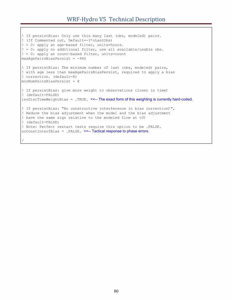
WRF-Hydro V5 Technical Description
! If persistBias: Only use this many last (obs, modeled) pairs.
! (If Commented out, Default=-1*nLastObs)
! > 0: apply an age-based filter, units=hours.
! = 0: apply no additional filter, use all available/usable obs.
! < 0: apply an count-based filter, units=count
maxAgePairsBiasPersist = -960
! If persistBias: The minimum number of last (obs, modeled) pairs,
! with age less than maxAgePairsBiasPersist, required to apply a bias
! correction. (default=8)
minNumPairsBiasPersist = 8
! If persistBias: give more weight to observations closer in time?
! (default=FALSE)
invDistTimeWeightBias = .TRUE. <<-- The exact form of this weighting is currently hard-coded.
! If persistBias: "No constructive interference in bias correction?",
! Reduce the bias adjustment when the model and the bias adjustment
! have the same sign relative to the modeled flow at t0?
! (default=FALSE)
! Note: Perfect restart tests require this option to be .FALSE.
noConstInterfBias = .FALSE. <<-- Tactical response to phase errors.
/
80
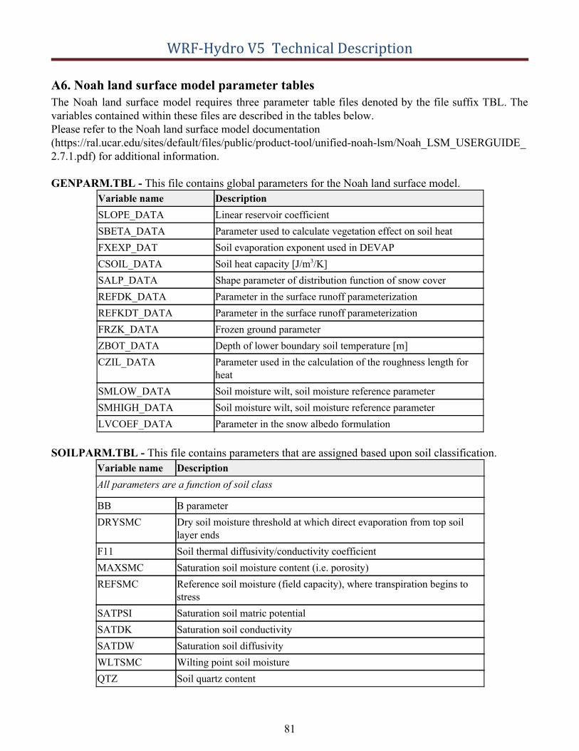
WRF-Hydro V5 Technical Description
A6. Noah land surface model parameter tables The Noah land surface model requires three parameter table files denoted by the file suffix TBL. The variables contained within these files are described in the tables below. Please refer to the Noah land surface model documentation (https://ral.ucar.edu/sites/default/files/public/product-tool/unified-noah-lsm/Noah_LSM_USERGUIDE_2.7.1.pdf) for additional information.
GENPARM.TBL - This file contains global parameters for the Noah land surface model. Variable name Description SLOPE_DATA Linear reservoir coefficient SBETA_DATA Parameter used to calculate vegetation effect on soil heat FXEXP_DAT Soil evaporation exponent used in DEVAP CSOIL_DATA Soil heat capacity [J/m3/K] SALP_DATA Shape parameter of distribution function of snow cover REFDK_DATA Parameter in the surface runoff parameterization REFKDT_DATA Parameter in the surface runoff parameterization FRZK_DATA Frozen ground parameter ZBOT_DATA Depth of lower boundary soil temperature [m] CZIL_DATA Parameter used in the calculation of the roughness length for
heat SMLOW_DATA Soil moisture wilt, soil moisture reference parameter SMHIGH_DATA Soil moisture wilt, soil moisture reference parameter LVCOEF_DATA Parameter in the snow albedo formulation
SOILPARM.TBL - This file contains parameters that are assigned based upon soil classification. Variable name Description All parameters are a function of soil class
BB B parameter DRYSMC Dry soil moisture threshold at which direct evaporation from top soil
layer ends F11 Soil thermal diffusivity/conductivity coefficient MAXSMC Saturation soil moisture content (i.e. porosity) REFSMC Reference soil moisture (field capacity), where transpiration begins to
stress SATPSI Saturation soil matric potential SATDK Saturation soil conductivity SATDW Saturation soil diffusivity WLTSMC Wilting point soil moisture QTZ Soil quartz content
81
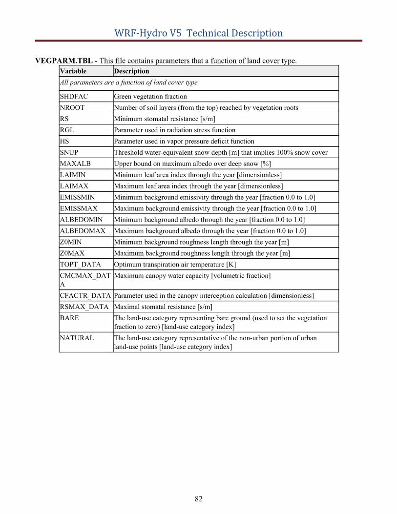
WRF-Hydro V5 Technical Description
VEGPARM.TBL - This file contains parameters that a function of land cover type. Variable Description All parameters are a function of land cover type
SHDFAC Green vegetation fraction NROOT Number of soil layers (from the top) reached by vegetation roots RS Minimum stomatal resistance [s/m] RGL Parameter used in radiation stress function HS Parameter used in vapor pressure deficit function SNUP Threshold water-equivalent snow depth [m] that implies 100% snow cover MAXALB Upper bound on maximum albedo over deep snow [%] LAIMIN Minimum leaf area index through the year [dimensionless] LAIMAX Maximum leaf area index through the year [dimensionless] EMISSMIN Minimum background emissivity through the year [fraction 0.0 to 1.0] EMISSMAX Maximum background emissivity through the year [fraction 0.0 to 1.0] ALBEDOMIN Minimum background albedo through the year [fraction 0.0 to 1.0] ALBEDOMAX Maximum background albedo through the year [fraction 0.0 to 1.0] Z0MIN Minimum background roughness length through the year [m] Z0MAX Maximum background roughness length through the year [m] TOPT_DATA Optimum transpiration air temperature [K] CMCMAX_DATA
Maximum canopy water capacity [volumetric fraction]
CFACTR_DATA Parameter used in the canopy interception calculation [dimensionless] RSMAX_DATA Maximal stomatal resistance [s/m] BARE The land-use category representing bare ground (used to set the vegetation
fraction to zero) [land-use category index] NATURAL The land-use category representative of the non-urban portion of urban
land-use points [land-use category index]
82
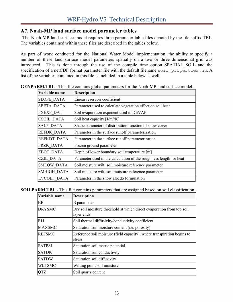
WRF-Hydro V5 Technical Description
A7. Noah-MP land surface model parameter tables The Noah-MP land surface model requires three parameter table files denoted by the file suffix TBL.
The variables contained within these files are described in the tables below.
As part of work conducted for the National Water Model implementation, the ability to specify a number of these land surface model parameters spatially on a two or three dimensional grid was introduced. This is done through the use of the compile time option SPATIAL_SOIL and the specification of a netCDF format parameter file with the default filename soil_properties.nc. A list of the variables contained in this file is included in a table below as well.
GENPARM.TBL - This file contains global parameters for the Noah-MP land surface model. Variable name Description SLOPE_DATA Linear reservoir coefficient SBETA_DATA Parameter used to calculate vegetation effect on soil heat FXEXP_DAT Soil evaporation exponent used in DEVAP CSOIL_DATA Soil heat capacity [J/m3/K] SALP_DATA Shape parameter of distribution function of snow cover REFDK_DATA Parameter in the surface runoff parameterization REFKDT_DATA Parameter in the surface runoff parameterization FRZK_DATA Frozen ground parameter ZBOT_DATA Depth of lower boundary soil temperature [m] CZIL_DATA Parameter used in the calculation of the roughness length for heat SMLOW_DATA Soil moisture wilt, soil moisture reference parameter SMHIGH_DATA Soil moisture wilt, soil moisture reference parameter LVCOEF_DATA Parameter in the snow albedo formulation
SOILPARM.TBL - This file contains parameters that are assigned based on soil classification. Variable name Description BB B parameter DRYSMC Dry soil moisture threshold at which direct evaporation from top soil
layer ends F11 Soil thermal diffusivity/conductivity coefficient MAXSMC Saturation soil moisture content (i.e. porosity) REFSMC Reference soil moisture (field capacity), where transpiration begins to
stress SATPSI Saturation soil matric potential SATDK Saturation soil conductivity SATDW Saturation soil diffusivity WLTSMC Wilting point soil moisture QTZ Soil quartz content
83
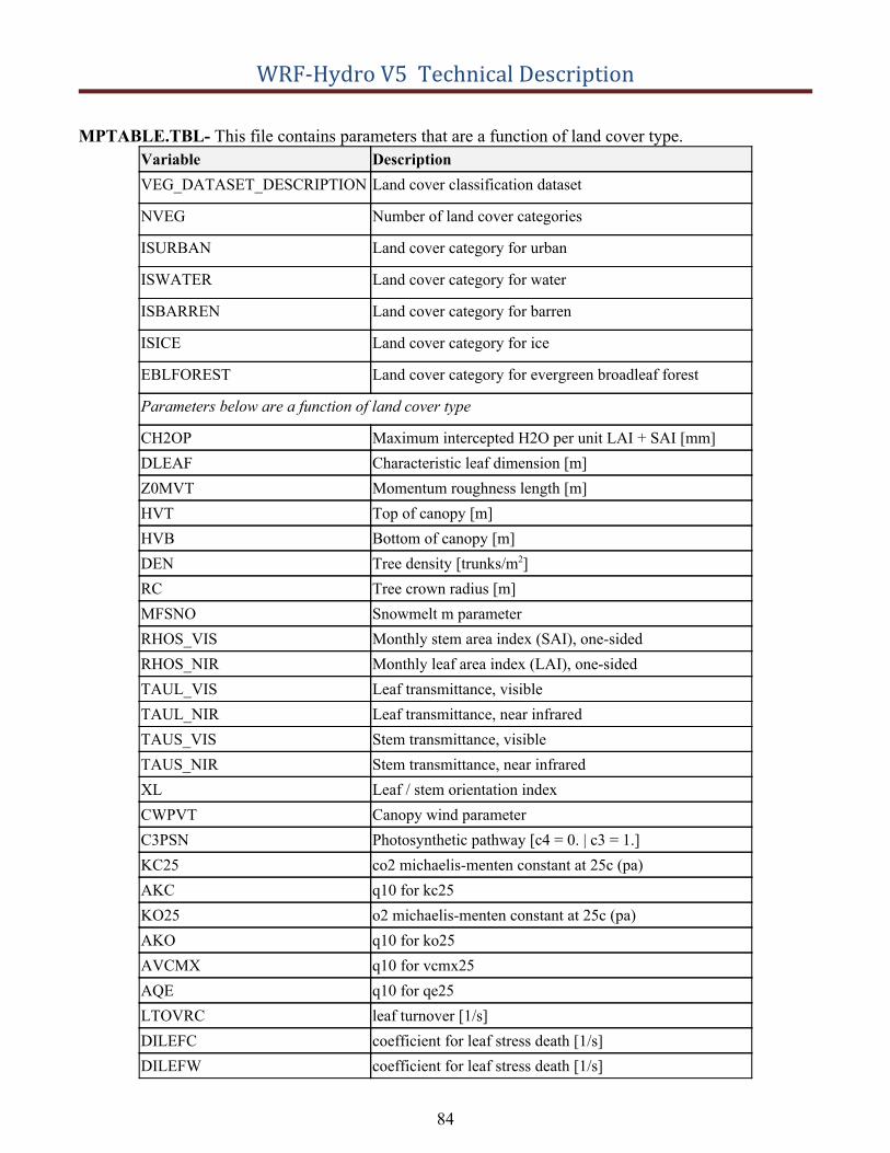
WRF-Hydro V5 Technical Description
MPTABLE.TBL- This file contains parameters that are a function of land cover type. Variable Description VEG_DATASET_DESCRIPTION Land cover classification dataset
NVEG Number of land cover categories
ISURBAN Land cover category for urban
ISWATER Land cover category for water
ISBARREN Land cover category for barren
ISICE Land cover category for ice
EBLFOREST Land cover category for evergreen broadleaf forest
Parameters below are a function of land cover type
CH2OP Maximum intercepted H2O per unit LAI + SAI [mm] DLEAF Characteristic leaf dimension [m] Z0MVT Momentum roughness length [m] HVT Top of canopy [m] HVB Bottom of canopy [m] DEN Tree density [trunks/m2] RC Tree crown radius [m] MFSNO Snowmelt m parameter RHOS_VIS Monthly stem area index (SAI), one-sided RHOS_NIR Monthly leaf area index (LAI), one-sided TAUL_VIS Leaf transmittance, visible TAUL_NIR Leaf transmittance, near infrared TAUS_VIS Stem transmittance, visible TAUS_NIR Stem transmittance, near infrared XL Leaf / stem orientation index CWPVT Canopy wind parameter C3PSN Photosynthetic pathway [c4 = 0. | c3 = 1.] KC25 co2 michaelis-menten constant at 25c (pa) AKC q10 for kc25 KO25 o2 michaelis-menten constant at 25c (pa) AKO q10 for ko25 AVCMX q10 for vcmx25 AQE q10 for qe25 LTOVRC leaf turnover [1/s] DILEFC coefficient for leaf stress death [1/s] DILEFW coefficient for leaf stress death [1/s]
84
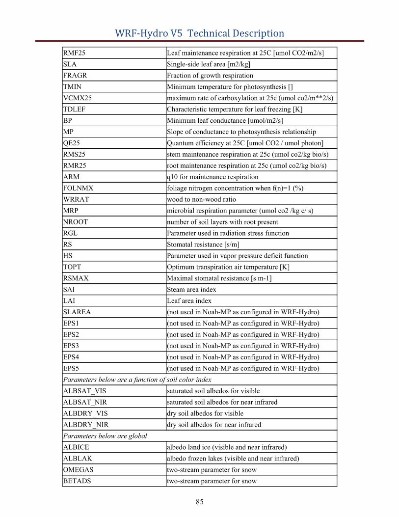
WRF-Hydro V5 Technical Description
RMF25 Leaf maintenance respiration at 25C [umol CO2/m2/s] SLA Single-side leaf area [m2/kg] FRAGR Fraction of growth respiration TMIN Minimum temperature for photosynthesis [] VCMX25 maximum rate of carboxylation at 25c (umol co2/m**2/s) TDLEF Characteristic temperature for leaf freezing [K] BP Minimum leaf conductance [umol/m2/s] MP Slope of conductance to photosynthesis relationship QE25 Quantum efficiency at 25C [umol CO2 / umol photon] RMS25 stem maintenance respiration at 25c (umol co2/kg bio/s) RMR25 root maintenance respiration at 25c (umol co2/kg bio/s) ARM q10 for maintenance respiration FOLNMX foliage nitrogen concentration when f(n)=1 (%) WRRAT wood to non-wood ratio MRP microbial respiration parameter (umol co2 /kg c/ s) NROOT number of soil layers with root present RGL Parameter used in radiation stress function RS Stomatal resistance [s/m] HS Parameter used in vapor pressure deficit function TOPT Optimum transpiration air temperature [K] RSMAX Maximal stomatal resistance [s m-1] SAI Steam area index LAI Leaf area index SLAREA (not used in Noah-MP as configured in WRF-Hydro) EPS1 (not used in Noah-MP as configured in WRF-Hydro) EPS2 (not used in Noah-MP as configured in WRF-Hydro) EPS3 (not used in Noah-MP as configured in WRF-Hydro) EPS4 (not used in Noah-MP as configured in WRF-Hydro) EPS5 (not used in Noah-MP as configured in WRF-Hydro) Parameters below are a function of soil color index ALBSAT_VIS saturated soil albedos for visible ALBSAT_NIR saturated soil albedos for near infrared ALBDRY_VIS dry soil albedos for visible ALBDRY_NIR dry soil albedos for near infrared Parameters below are global ALBICE albedo land ice (visible and near infrared) ALBLAK albedo frozen lakes (visible and near infrared) OMEGAS two-stream parameter for snow BETADS two-stream parameter for snow
85
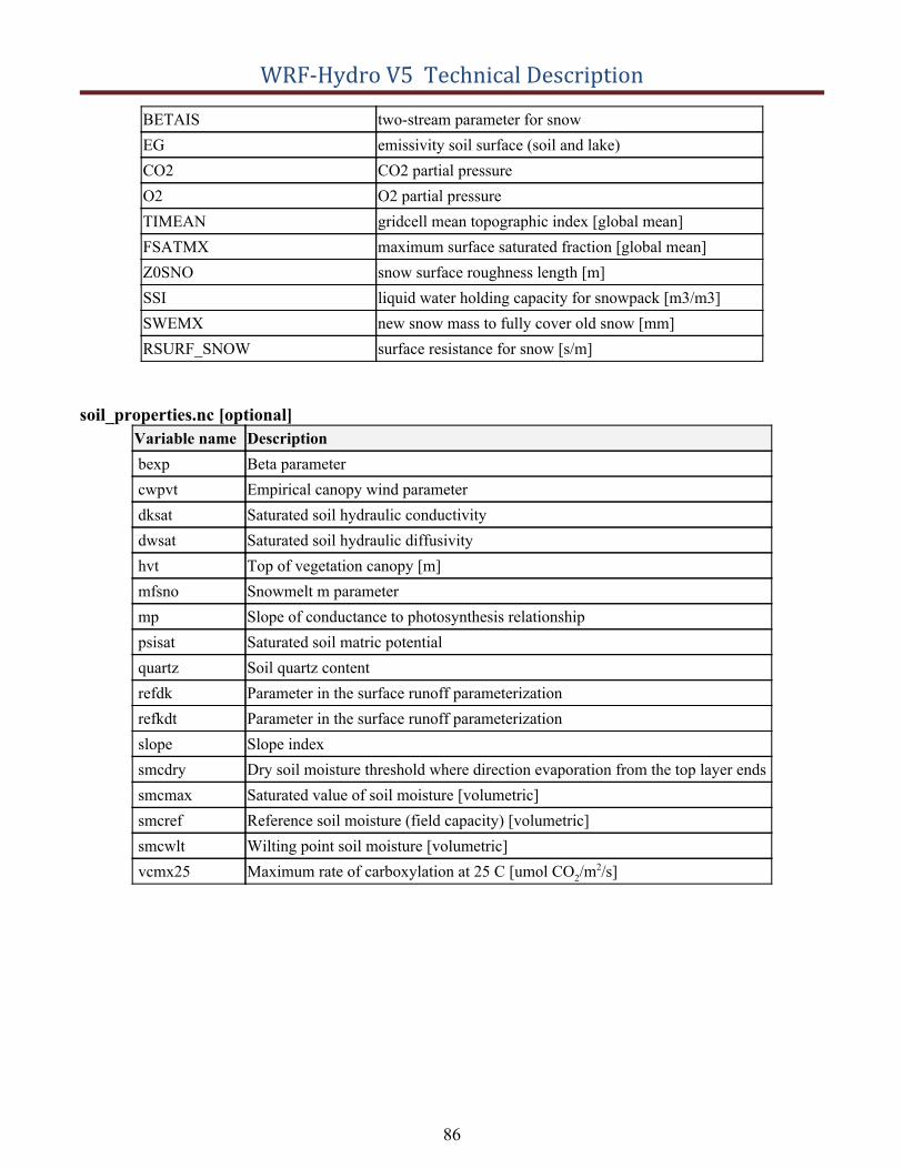
WRF-Hydro V5 Technical Description
BETAIS two-stream parameter for snow EG emissivity soil surface (soil and lake) CO2 CO2 partial pressure O2 O2 partial pressure TIMEAN gridcell mean topographic index [global mean] FSATMX maximum surface saturated fraction [global mean] Z0SNO snow surface roughness length [m] SSI liquid water holding capacity for snowpack [m3/m3] SWEMX new snow mass to fully cover old snow [mm] RSURF_SNOW surface resistance for snow [s/m]
soil_properties.nc [optional] Variable name Description bexp Beta parameter cwpvt Empirical canopy wind parameter dksat Saturated soil hydraulic conductivity dwsat Saturated soil hydraulic diffusivity hvt Top of vegetation canopy [m] mfsno Snowmelt m parameter mp Slope of conductance to photosynthesis relationship psisat Saturated soil matric potential quartz Soil quartz content refdk Parameter in the surface runoff parameterization refkdt Parameter in the surface runoff parameterization slope Slope index smcdry Dry soil moisture threshold where direction evaporation from the top layer ends smcmax Saturated value of soil moisture [volumetric] smcref Reference soil moisture (field capacity) [volumetric] smcwlt Wilting point soil moisture [volumetric] vcmx25 Maximum rate of carboxylation at 25 C [umol CO2/m2/s]
86
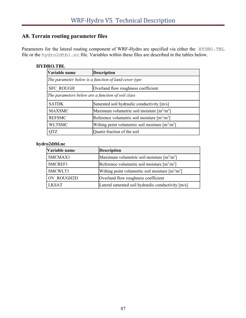
WRF-Hydro V5 Technical Description
A8. Terrain routing parameter files
Parameters for the lateral routing component of WRF-Hydro are specified via either the HYDRO.TBL file or the hydro2dtbl.nc file. Variables within these files are described in the tables below.
HYDRO.TBL Variable name Description The parameter below is a function of land cover type
SFC_ROUGH Overland flow roughness coefficient The parameters below are a function of soil class
SATDK Saturated soil hydraulic conductivity [m/s] MAXSMC Maximum volumetric soil moisture [m3/m3] REFSMC Reference volumetric soil moisture [m3/m3] WLTSMC Wilting point volumetric soil moisture [m3/m3] QTZ Quartz fraction of the soil
hydro2dtbl.nc Variable name Description SMCMAX1 Maximum volumetric soil moisture [m3/m3] SMCREF1 Reference volumetric soil moisture [m3/m3] SMCWLT1 Wilting point volumetric soil moisture [m3/m3] OV_ROUGH2D Overland flow roughness coefficient LKSAT Lateral saturated soil hydraulic conductivity [m/s]
87
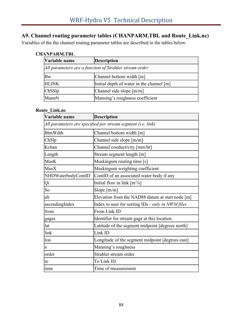
WRF-Hydro V5 Technical Description
A9. Channel routing parameter tables (CHANPARM.TBL and Route_Link.nc) Variables of the the channel routing parameter tables are described in the tables below.
CHANPARM.TBL Variable name Description All parameters are a function of Strahler stream order
Bw Channel bottom width [m] HLINK Initial depth of water in the channel [m] ChSSlp Channel side slope [m/m] MannN Manning’s roughness coefficient
Route_Link.nc Variable name Description All parameters are specified per stream segment (i.e. link)
BtmWdth Channel bottom width [m] ChSlp Channel side slope [m/m] Kchan Channel conductivity [mm/hr] Length Stream segment length [m] MusK Muskingum routing time [s] MusX Muskingum weighting coefficient NHDWaterbodyComID ComID of an associated water body if any Qi Initial flow in link [m3/s] So Slope [m/m] alt Elevation from the NAD88 datum at start node [m] ascendingIndex Index to user for sorting IDs - only in NWM files from From Link ID gages Identifier for stream gage at this location lat Latitude of the segment midpoint [degrees north] link Link ID lon Longitude of the segment midpoint [degrees east] n Manning’s roughness order Strahler stream order to To Link ID time Time of measurement
88

WRF-Hydro V5 Technical Description
A10. Groundwater input and parameter files The contents of the groundwater input and parameter files are described in the tables below.
GWBASINS.nc Variable name Description y projection y coordinate x projection x coordinate crs coordinate reference system definition BASIN groundwater basin ID
GWBUCKPARM.nc Variable name Basin Coeff Expon Zmax Zinit Area_sqkm ComID
Description Basin monotonic ID (1...n) Coefficient Exponent Zmax Zinit Basin area in square kilometers NHDCatchment FEATUREID (NHDFlowline ComID)
89
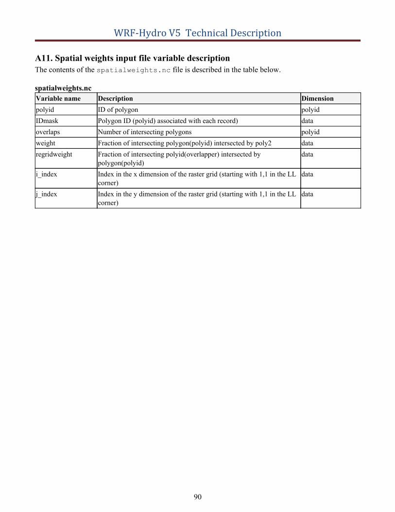
WRF-Hydro V5 Technical Description
A11. Spatial weights input file variable description The contents of the spatialweights.nc file is described in the table below.
spatialweights.nc Variable name Description Dimension polyid ID of polygon polyid IDmask Polygon ID (polyid) associated with each record) data overlaps Number of intersecting polygons polyid weight Fraction of intersecting polygon(polyid) intersected by poly2 data regridweight Fraction of intersecting polyid(overlapper) intersected by
polygon(polyid) data
i_index Index in the x dimension of the raster grid (starting with 1,1 in the LL corner)
data
j_index Index in the y dimension of the raster grid (starting with 1,1 in the LL corner)
data
90
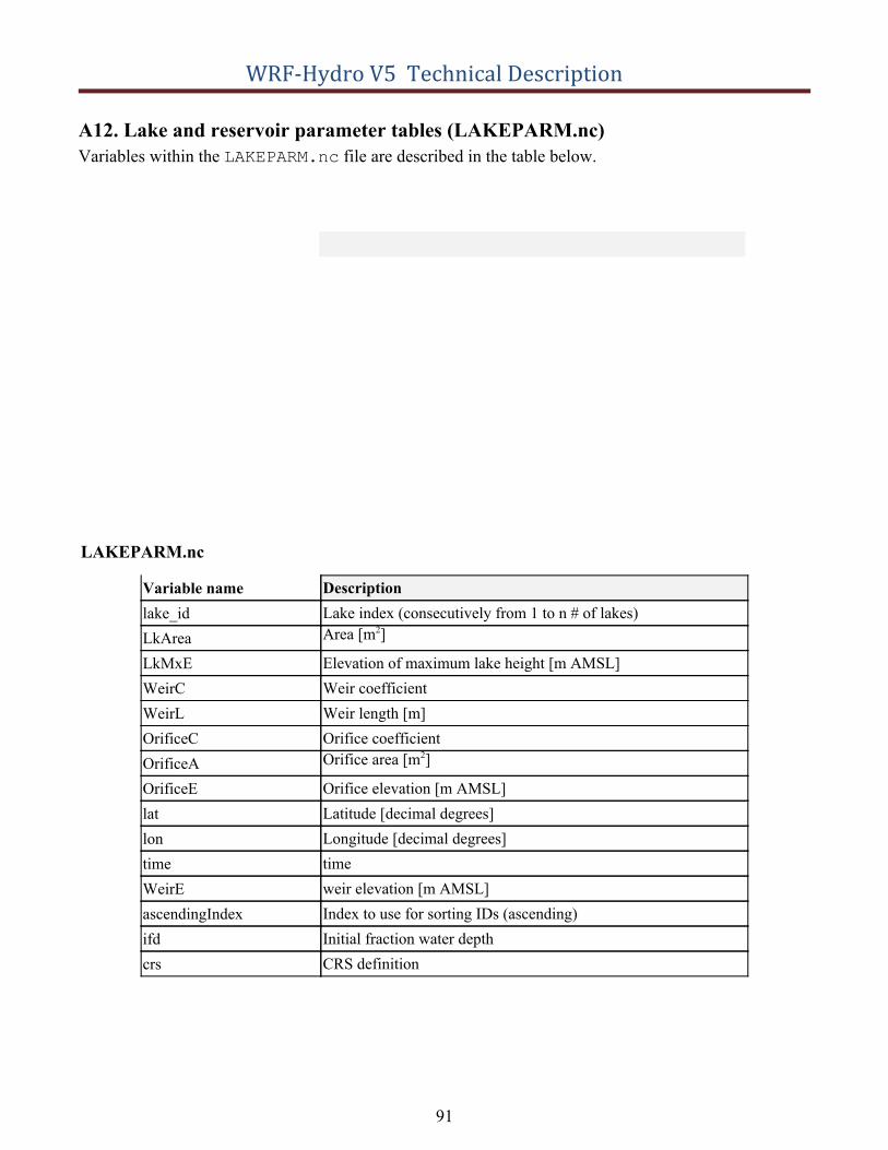
WRF-Hydro V5 Technical Description
A12. Lake and reservoir parameter tables (LAKEPARM.nc) Variables within the LAKEPARM.nc file are described in the table below.
LAKEPARM.nc
Variable name lake_id LkArea LkMxE WeirC WeirL OrificeC OrificeA OrificeE lat lon time WeirE ascendingIndex ifd crs
Description Lake index (consecutively from 1 to n # of lakes) Area [m2]
Elevation of maximum lake height [m AMSL] Weir coefficient Weir length [m] Orifice coefficient Orifice area [m 2 ]
Orifice elevation [m AMSL] Latitude [decimal degrees] Longitude [decimal degrees] time weir elevation [m AMSL] Index to use for sorting IDs (ascending) Initial fraction water depth CRS definition
91
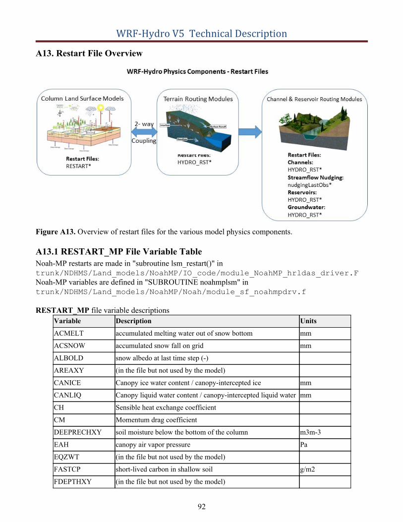
WRF-Hydro V5 Technical Description
A13. Restart File Overview
Figure A13. Overview of restart files for the various model physics components.
A13.1 RESTART_MP File Variable Table Noah-MP restarts are made in "subroutine lsm_restart()" in trunk/NDHMS/Land_models/NoahMP/IO_code/module_NoahMP_hrldas_driver.F
Noah-MP variables are defined in "SUBROUTINE noahmplsm" in trunk/NDHMS/Land_models/NoahMP/Noah/module_sf_noahmpdrv.f
RESTART_MP file variable descriptions Variable Description Units
ACMELT accumulated melting water out of snow bottom mm
ACSNOW accumulated snow fall on grid mm
ALBOLD snow albedo at last time step (-)
AREAXY (in the file but not used by the model)
CANICE Canopy ice water content / canopy-intercepted ice mm
CANLIQ Canopy liquid water content / canopy-intercepted liquid water mm
CH Sensible heat exchange coefficient
CM Momentum drag coefficient
DEEPRECHXY soil moisture below the bottom of the column m3m-3
EAH canopy air vapor pressure Pa
EQZWT (in the file but not used by the model)
FASTCP short-lived carbon in shallow soil g/m2
FDEPTHXY (in the file but not used by the model)
92
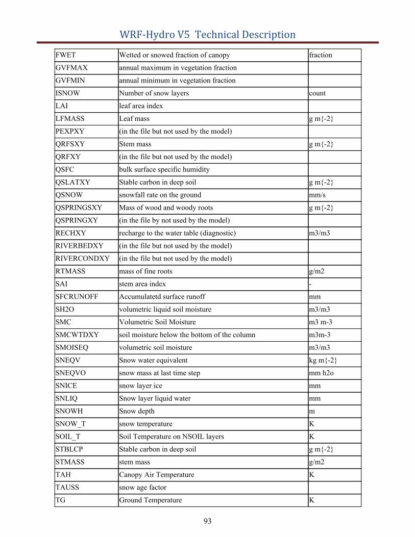
WRF-Hydro V5 Technical Description
FWET Wetted or snowed fraction of canopy fraction
GVFMAX annual maximum in vegetation fraction
GVFMIN annual minimum in vegetation fraction
ISNOW Number of snow layers count
LAI leaf area index
LFMASS Leaf mass g m{-2}
PEXPXY (in the file but not used by the model)
QRFSXY Stem mass g m{-2}
QRFXY (in the file but not used by the model)
QSFC bulk surface specific humidity
QSLATXY Stable carbon in deep soil g m{-2}
QSNOW snowfall rate on the ground mm/s
QSPRINGSXY Mass of wood and woody roots g m{-2}
QSPRINGXY (in the file by not used by the model)
RECHXY recharge to the water table (diagnostic) m3/m3
RIVERBEDXY (in the file but not used by the model)
RIVERCONDXY (in the file but not used by the model)
RTMASS mass of fine roots g/m2
SAI stem area index -
SFCRUNOFF Accumulatetd surface runoff mm
SH2O volumetric liquid soil moisture m3/m3
SMC Volumetric Soil Moisture m3 m-3
SMCWTDXY soil moisture below the bottom of the column m3m-3
SMOISEQ volumetric soil moisture m3/m3
SNEQV Snow water equivalent kg m{-2}
SNEQVO snow mass at last time step mm h2o
SNICE snow layer ice mm
SNLIQ Snow layer liquid water mm
SNOWH Snow depth m
SNOW_T snow temperature K
SOIL_T Soil Temperature on NSOIL layers K
STBLCP Stable carbon in deep soil g m{-2}
STMASS stem mass g/m2
TAH Canopy Air Temperature K
TAUSS snow age factor
TG Ground Temperature K
93
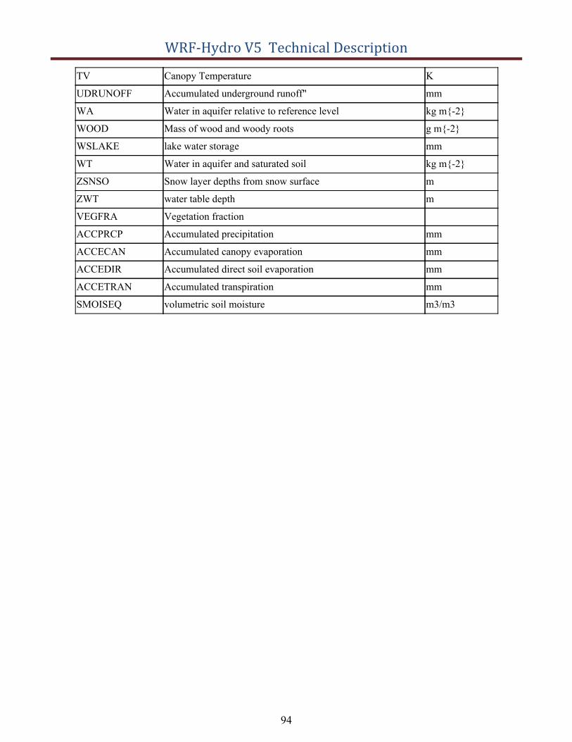
WRF-Hydro V5 Technical Description
TV Canopy Temperature K
UDRUNOFF Accumulated underground runoff" mm
WA Water in aquifer relative to reference level kg m{-2}
WOOD Mass of wood and woody roots g m{-2}
WSLAKE lake water storage mm
WT Water in aquifer and saturated soil kg m{-2}
ZSNSO Snow layer depths from snow surface m
ZWT water table depth m
VEGFRA Vegetation fraction
ACCPRCP Accumulated precipitation mm
ACCECAN Accumulated canopy evaporation mm
ACCEDIR Accumulated direct soil evaporation mm
ACCETRAN Accumulated transpiration mm
SMOISEQ volumetric soil moisture m3/m3
94
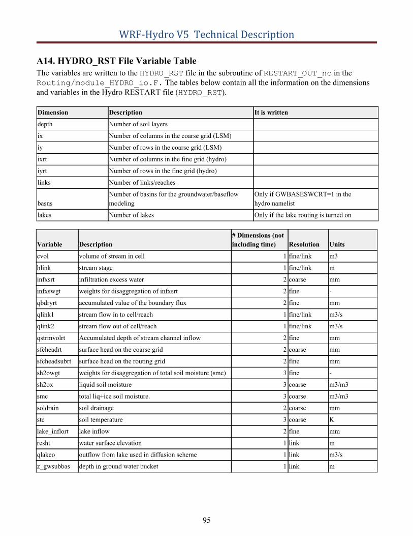
WRF-Hydro V5 Technical Description
A14. HYDRO_RST File Variable Table The variables are written to the HYDRO_RST file in the subroutine of RESTART_OUT_nc in theRouting/module_HYDRO_io.F. The tables below contain all the information on the dimensionsand variables in the Hydro RESTART file ( HYDRO_RST).
Dimension Description It is written
depth Number of soil layers
ix Number of columns in the coarse grid (LSM)
iy Number of rows in the coarse grid (LSM)
ixrt Number of columns in the fine grid (hydro)
iyrt Number of rows in the fine grid (hydro)
links Number of links/reaches
basns Number of basins for the groundwater/baseflow modeling
Only if GWBASESWCRT=1 in the hydro.namelist
lakes Number of lakes Only if the lake routing is turned on
Variable Description # Dimensions (not including time) Resolution Units
cvol volume of stream in cell 1 fine/link m3
hlink stream stage 1 fine/link m
infxsrt infiltration excess water 2 coarse mm
infxswgt weights for disaggregation of infxsrt 2 fine -
qbdryrt accumulated value of the boundary flux 2 fine mm
qlink1 stream flow in to cell/reach 1 fine/link m3/s
qlink2 stream flow out of cell/reach 1 fine/link m3/s
qstrmvolrt Accumulated depth of stream channel inflow 2 fine mm
sfcheadrt surface head on the coarse grid 2 coarse mm
sfcheadsubrt surface head on the routing grid 2 fine mm
sh2owgt weights for disaggregation of total soil moisture (smc) 3 fine -
sh2ox liquid soil moisture 3 coarse m3/m3
smc total liq+ice soil moisture. 3 coarse m3/m3
soldrain soil drainage 2 coarse mm
stc soil temperature 3 coarse K
lake_inflort lake inflow 2 fine mm
resht water surface elevation 1 link m
qlakeo outflow from lake used in diffusion scheme 1 link m3/s
z_gwsubbas depth in ground water bucket 1 link m
95
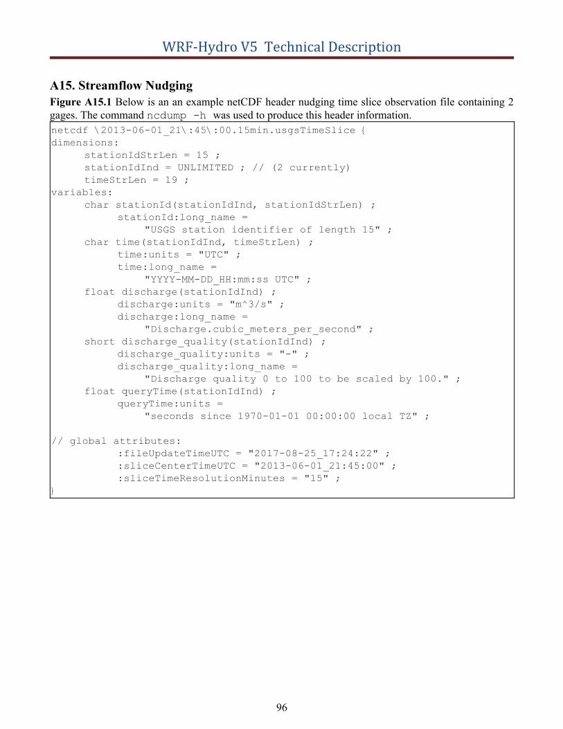
WRF-Hydro V5 Technical Description
A15. Streamflow Nudging Figure A15.1 Below is an an example netCDF header nudging time slice observation file containing 2 gages. The command ncdump -h was used to produce this header information.netcdf \2013-06-01_21\:45\:00.15min.usgsTimeSlice {
dimensions:
stationIdStrLen = 15 ;
stationIdInd = UNLIMITED ; // (2 currently)
timeStrLen = 19 ;
variables:
char stationId(stationIdInd, stationIdStrLen) ;
stationId:long_name =
"USGS station identifier of length 15" ;
char time(stationIdInd, timeStrLen) ;
time:units = "UTC" ;
time:long_name =
"YYYY-MM-DD_HH:mm:ss UTC" ;
float discharge(stationIdInd) ;
discharge:units = "m^3/s" ;
discharge:long_name =
"Discharge.cubic_meters_per_second" ;
short discharge_quality(stationIdInd) ;
discharge_quality:units = "-" ;
discharge_quality:long_name =
"Discharge quality 0 to 100 to be scaled by 100." ;
float queryTime(stationIdInd) ;
queryTime:units =
"seconds since 1970-01-01 00:00:00 local TZ" ;
// global attributes:
:fileUpdateTimeUTC = "2017-08-25_17:24:22" ;
:sliceCenterTimeUTC = "2013-06-01_21:45:00" ;
:sliceTimeResolutionMinutes = "15" ;
}
96
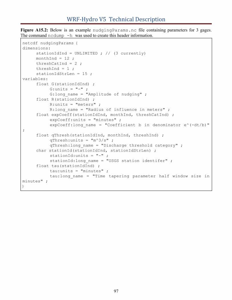
WRF-Hydro V5 Technical Description
Figure A15.2: Below is an example nudgingParams.nc file containing parameters for 3 gages. The command ncdump -h was used to create this header information.netcdf nudgingParams {
dimensions:
stationIdInd = UNLIMITED ; // (3 currently)
monthInd = 12 ;
threshCatInd = 2 ;
threshInd = 1 ;
stationIdStrLen = 15 ;
variables:
float G(stationIdInd) ;
G:units = "-" ;
G:long_name = "Amplitude of nudging" ;
float R(stationIdInd) ;
R:units = "meters" ;
R:long_name = "Radius of influence in meters" ;
float expCoeff(stationIdInd, monthInd, threshCatInd) ;
expCoeff:units = "minutes" ;
expCoeff:long_name = "Coefficient b in denominator e^(-dt/b)"
;
float qThresh(stationIdInd, monthInd, threshInd) ;
qThresh:units = "m^3/s" ;
qThresh:long_name = "Discharge threshold category" ;
char stationId(stationIdInd, stationIdStrLen) ;
stationId:units = "-" ;
stationId:long_name = "USGS station identifer" ;
float tau(stationIdInd) ;
tau:units = "minutes" ;
tau:long_name = "Time tapering parameter half window size in
minutes" ;
}
97

WRF-Hydro V5 Technical Description
A16. National Water Model (NWM) Configuration It is important to note here that the community WRF-Hydro modeling system is currently the actual modeling architecture that is used in the NOAA National Water Model. This means that the community WRF-Hydro model code is configurable into the National Water Model configurations that run in operations at the National Center for Environmental Prediction (NCEP).
“The NWM is an hourly cycling uncoupled analysis and forecast system that provides streamflow for 2.7 million river reaches and other hydrologic information on 1km and 250m grids. The model provides complementary hydrologic guidance at current NWS River Forecast Center river forecast locations and significantly expanded guidance coverage and type in underserved locations.
The NWM ingests forcing from a variety of sources including Multi-Radar Multi-Sensor (MRMS) radar-gauge observed precipitation data and High-Resolution Rapid Refresh (HRRR), Rapid Refresh (RAP), Global Forecast System (GFS) and Climate Forecast System (CFS) Numerical Weather Prediction (NWP) forecast data. USGS real-time streamflow observations are assimilated and all NWM configurations benefit from the inclusion of ~1,500 reservoirs. The core of the NWM system is the National Center for Atmospheric Research (NCAR)-supported community Weather Research and Forecasting (WRF)-Hydro hydrologic model. WRF-Hydro is configured to use the Noah Multi- Parameterization (Noah-MP) Land Surface Model (LSM) to simulate land surface processes. Separate water routing modules perform diffusive wave surface routing and saturated subsurface flow routing on a 250m grid, and Muskingum-Cunge channel routing down NHDPlusV2 stream reaches. River analyses and forecasts are provided across a domain encompassing the continental U.S. and hydrologically-contributing areas, while land surface output is available on a larger domain that extends beyond the continental U.S. into Canada and Mexico (roughly from latitude 19N to 58N). In addition, NWM forcing datasets are provided on this domain at a resolution of 1km.”
Excerpt from NOUS41 KWBC 061735 PNSWSH NWS Office of Science and Technology Integration
For more information regarding the operational configuration, input, and output data of the National Water Model see the Office of Water Prediction website: http://water.noaa.gov/about/nwm and the Open Commons Consortium Environmental Data Commons website: http://edc.occ-data.org/nwm/.
The NWM/WRF-Hydro modeling system suite of tools for data preparation, evaluation, and calibration. is continually under development and will be rolled out to the community as each tool becomes finalized with supporting documentation for public usage. To be notified when tools become available please subscribe to the WRF-Hydro email list https://ral.ucar.edu/projects/wrf_hydro/subscribe.
The figures below illustrate the physics permutations available in the WRF-Hydro framework and the Noah-MP land surface model as well as the current National Water Model configuration as of March 2018, the NWM ecosystem and suite of tools and sample NWM configuration namelists.
98
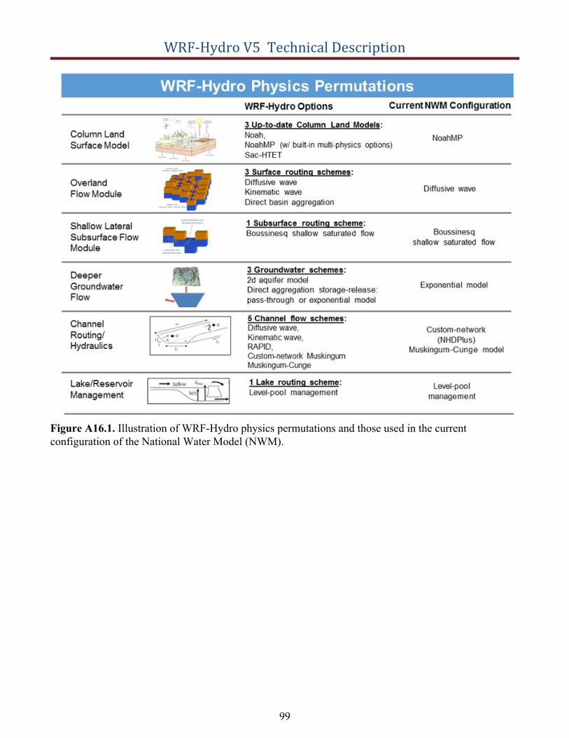
WRF-Hydro V5 Technical Description
Figure A16.1. Illustration of WRF-Hydro physics permutations and those used in the current configuration of the National Water Model (NWM).
99
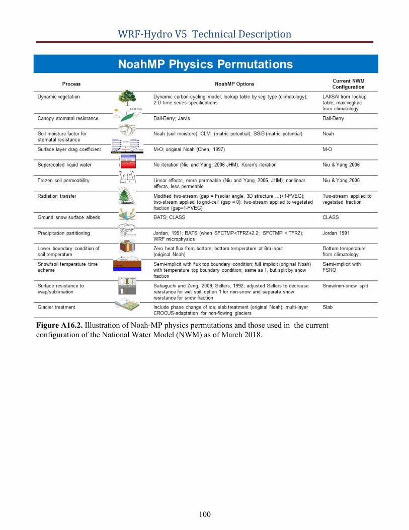
WRF-Hydro V5 Technical Description
Figure A16.2. Illustration of Noah-MP physics permutations and those used in the current configuration of the National Water Model (NWM) as of March 2018.
100
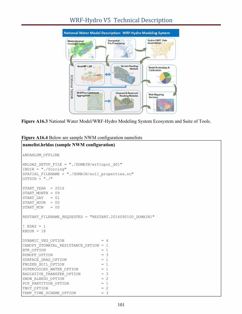
WRF-Hydro V5 Technical Description
Figure A16.3 National Water Model/WRF-Hydro Modeling System Ecosystem and Suite of Tools.
Figure A16.4 Below are sample NWM configuration namelists namelist.hrldas (sample NWM configuration)
&NOAHLSM_OFFLINE
HRLDAS_SETUP_FILE = "./DOMAIN/wrfinput_d01"
INDIR = "./forcing"
SPATIAL_FILENAME = "./DOMAIN/soil_properties.nc"
OUTDIR = "./"
START_YEAR = 2016
START_MONTH = 09
START_DAY = 01
START_HOUR = 00
START_MIN = 00
RESTART_FILENAME_REQUESTED = "RESTART.2016090100_DOMAIN1"
! KDAY = 1
KHOUR = 18
DYNAMIC_VEG_OPTION = 4
CANOPY_STOMATAL_RESISTANCE_OPTION = 1
BTR_OPTION = 1
RUNOFF_OPTION = 3
SURFACE_DRAG_OPTION = 1
FROZEN_SOIL_OPTION = 1
SUPERCOOLED_WATER_OPTION = 1
RADIATIVE_TRANSFER_OPTION = 3
SNOW_ALBEDO_OPTION = 2
PCP_PARTITION_OPTION = 1
TBOT_OPTION = 2
TEMP_TIME_SCHEME_OPTION = 3
101
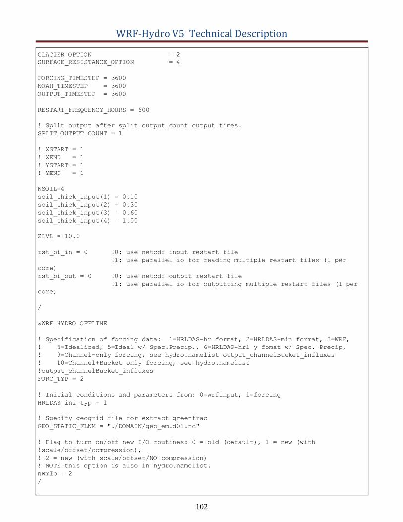
WRF-Hydro V5 Technical Description
GLACIER_OPTION = 2
SURFACE_RESISTANCE_OPTION = 4
FORCING_TIMESTEP = 3600
NOAH_TIMESTEP = 3600
OUTPUT_TIMESTEP = 3600
RESTART_FREQUENCY_HOURS = 600
! Split output after split_output_count output times.
SPLIT_OUTPUT_COUNT = 1
! XSTART = 1
! XEND = 1
! YSTART = 1
! YEND = 1
NSOIL=4
soil_thick_input(1) = 0.10
soil_thick_input(2) = 0.30
soil_thick_input(3) = 0.60
soil_thick_input(4) = 1.00
ZLVL = 10.0
rst_bi_in = 0 !0: use netcdf input restart file
!1: use parallel io for reading multiple restart files (1 per
core)
rst_bi_out = 0 !0: use netcdf output restart file
!1: use parallel io for outputting multiple restart files (1 per
core)
/
&WRF_HYDRO_OFFLINE
! Specification of forcing data: 1=HRLDAS-hr format, 2=HRLDAS-min format, 3=WRF,
! 4=Idealized, 5=Ideal w/ Spec.Precip., 6=HRLDAS-hrl y fomat w/ Spec. Precip,
! 9=Channel-only forcing, see hydro.namelist output_channelBucket_influxes
! 10=Channel+Bucket only forcing, see hydro.namelist
!output_channelBucket_influxes
FORC_TYP = 2
! Initial conditions and parameters from: 0=wrfinput, 1=forcing
HRLDAS_ini_typ = 1
! Specify geogrid file for extract greenfrac
GEO_STATIC_FLNM = "./DOMAIN/geo_em.d01.nc"
! Flag to turn on/off new I/O routines: 0 = old (default), 1 = new (with
!scale/offset/compression),
! 2 = new (with scale/offset/NO compression)
! NOTE this option is also in hydro.namelist.
nwmIo = 2
/
102
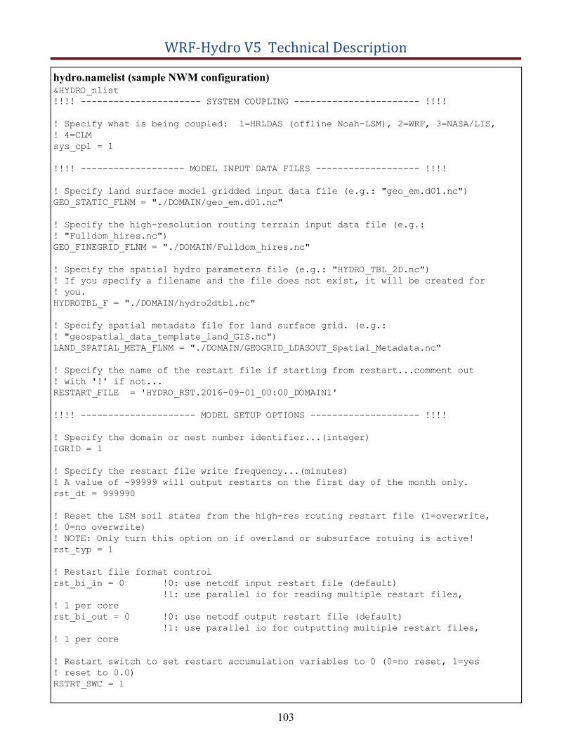
WRF-Hydro V5 Technical Description
hydro.namelist (sample NWM configuration) &HYDRO_nlist
!!!! ---------------------- SYSTEM COUPLING ----------------------- !!!!
! Specify what is being coupled: 1=HRLDAS (offline Noah-LSM), 2=WRF, 3=NASA/LIS,
! 4=CLM
sys_cpl = 1
!!!! ------------------- MODEL INPUT DATA FILES ------------------- !!!!
! Specify land surface model gridded input data file (e.g.: "geo_em.d01.nc")
GEO_STATIC_FLNM = "./DOMAIN/geo_em.d01.nc"
! Specify the high-resolution routing terrain input data file (e.g.:
! "Fulldom_hires.nc")
GEO_FINEGRID_FLNM = "./DOMAIN/Fulldom_hires.nc"
! Specify the spatial hydro parameters file (e.g.: "HYDRO_TBL_2D.nc")
! If you specify a filename and the file does not exist, it will be created for
! you.
HYDROTBL_F = "./DOMAIN/hydro2dtbl.nc"
! Specify spatial metadata file for land surface grid. (e.g.:
! "geospatial_data_template_land_GIS.nc")
LAND_SPATIAL_META_FLNM = "./DOMAIN/GEOGRID_LDASOUT_Spatial_Metadata.nc"
! Specify the name of the restart file if starting from restart...comment out
! with '!' if not...
RESTART_FILE = 'HYDRO_RST.2016-09-01_00:00_DOMAIN1'
!!!! --------------------- MODEL SETUP OPTIONS -------------------- !!!!
! Specify the domain or nest number identifier...(integer)
IGRID = 1
! Specify the restart file write frequency...(minutes)
! A value of -99999 will output restarts on the first day of the month only.
rst_dt = 999990
! Reset the LSM soil states from the high-res routing restart file (1=overwrite,
! 0=no overwrite)
! NOTE: Only turn this option on if overland or subsurface rotuing is active!
rst_typ = 1
! Restart file format control
rst_bi_in = 0 !0: use netcdf input restart file (default)
!1: use parallel io for reading multiple restart files,
! 1 per core
rst_bi_out = 0 !0: use netcdf output restart file (default)
!1: use parallel io for outputting multiple restart files,
! 1 per core
! Restart switch to set restart accumulation variables to 0 (0=no reset, 1=yes
! reset to 0.0)
RSTRT_SWC = 1
103
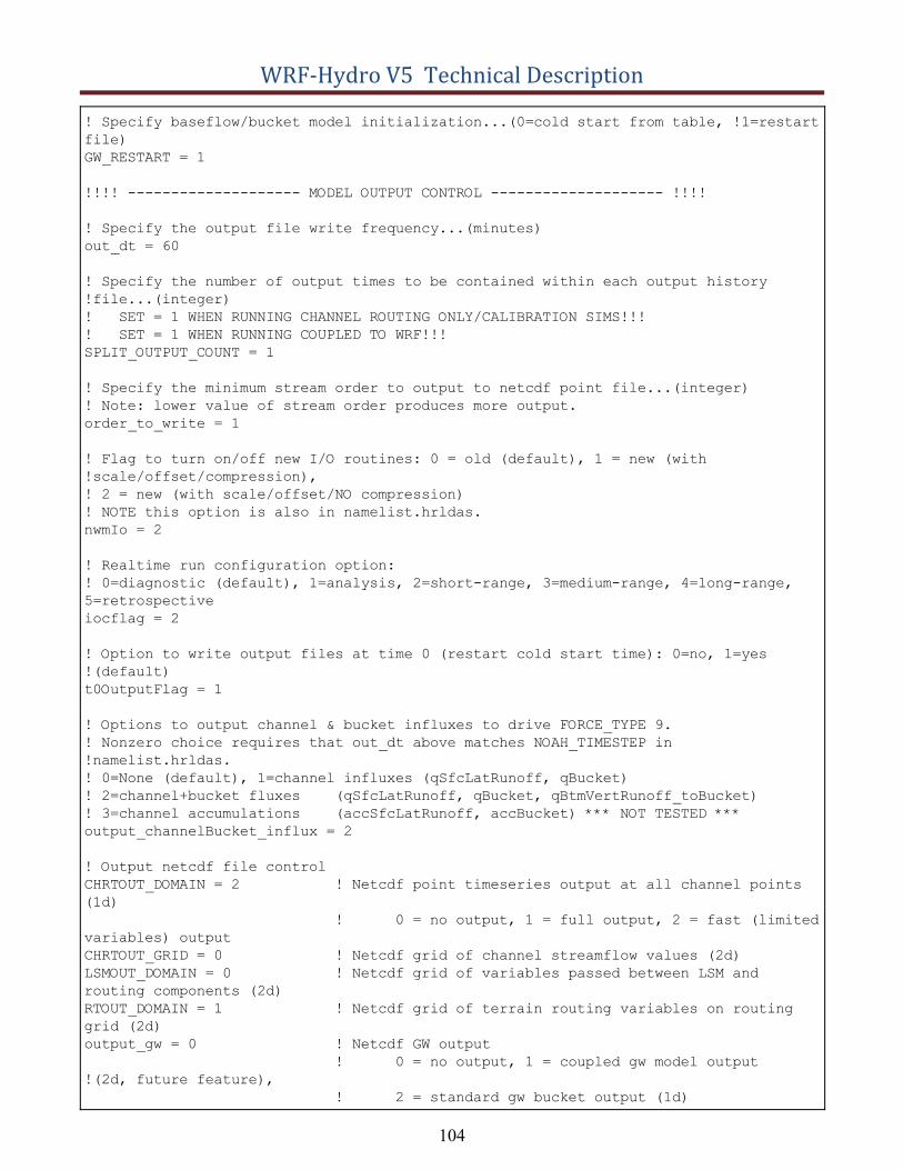
WRF-Hydro V5 Technical Description
! Specify baseflow/bucket model initialization...(0=cold start from table, !1=restart
file)
GW_RESTART = 1
!!!! -------------------- MODEL OUTPUT CONTROL -------------------- !!!!
! Specify the output file write frequency...(minutes)
out_dt = 60
! Specify the number of output times to be contained within each output history
!file...(integer)
! SET = 1 WHEN RUNNING CHANNEL ROUTING ONLY/CALIBRATION SIMS!!!
! SET = 1 WHEN RUNNING COUPLED TO WRF!!!
SPLIT_OUTPUT_COUNT = 1
! Specify the minimum stream order to output to netcdf point file...(integer)
! Note: lower value of stream order produces more output.
order_to_write = 1
! Flag to turn on/off new I/O routines: 0 = old (default), 1 = new (with
!scale/offset/compression),
! 2 = new (with scale/offset/NO compression)
! NOTE this option is also in namelist.hrldas.
nwmIo = 2
! Realtime run configuration option:
! 0=diagnostic (default), 1=analysis, 2=short-range, 3=medium-range, 4=long-range,
5=retrospective
iocflag = 2
! Option to write output files at time 0 (restart cold start time): 0=no, 1=yes
!(default)
t0OutputFlag = 1
! Options to output channel & bucket influxes to drive FORCE_TYPE 9.
! Nonzero choice requires that out_dt above matches NOAH_TIMESTEP in
!namelist.hrldas.
! 0=None (default), 1=channel influxes (qSfcLatRunoff, qBucket)
! 2=channel+bucket fluxes (qSfcLatRunoff, qBucket, qBtmVertRunoff_toBucket)
! 3=channel accumulations (accSfcLatRunoff, accBucket) *** NOT TESTED ***
output_channelBucket_influx = 2
! Output netcdf file control
CHRTOUT_DOMAIN = 2 ! Netcdf point timeseries output at all channel points
(1d)
! 0 = no output, 1 = full output, 2 = fast (limited
variables) output
CHRTOUT_GRID = 0 ! Netcdf grid of channel streamflow values (2d)
LSMOUT_DOMAIN = 0 ! Netcdf grid of variables passed between LSM and
routing components (2d)
RTOUT_DOMAIN = 1 ! Netcdf grid of terrain routing variables on routing
grid (2d)
output_gw = 0 ! Netcdf GW output
! 0 = no output, 1 = coupled gw model output
!(2d, future feature),
! 2 = standard gw bucket output (1d)
104
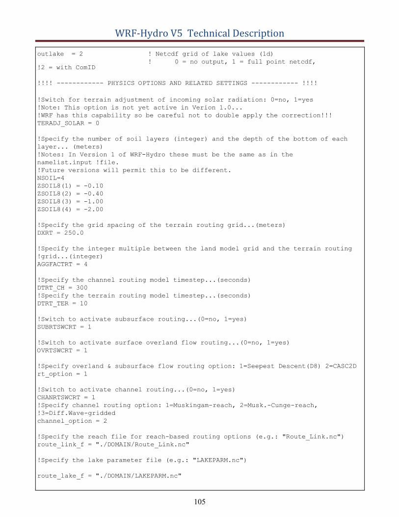
WRF-Hydro V5 Technical Description
outlake = 2 ! Netcdf grid of lake values (1d)
! 0 = no output, 1 = full point netcdf,
!2 = with ComID
!!!! ------------ PHYSICS OPTIONS AND RELATED SETTINGS ------------ !!!!
!Switch for terrain adjustment of incoming solar radiation: 0=no, 1=yes
!Note: This option is not yet active in Verion 1.0...
!WRF has this capability so be careful not to double apply the correction!!!
TERADJ_SOLAR = 0
!Specify the number of soil layers (integer) and the depth of the bottom of each
layer... (meters)
!Notes: In Version 1 of WRF-Hydro these must be the same as in the
namelist.input !file.
!Future versions will permit this to be different.
NSOIL=4
ZSOIL8(1) = -0.10
ZSOIL8(2) = -0.40
ZSOIL8(3) = -1.00
ZSOIL8(4) = -2.00
!Specify the grid spacing of the terrain routing grid...(meters)
DXRT = 250.0
!Specify the integer multiple between the land model grid and the terrain routing
!grid...(integer)
AGGFACTRT = 4
!Specify the channel routing model timestep...(seconds)
DTRT_CH = 300
!Specify the terrain routing model timestep...(seconds)
DTRT_TER = 10
!Switch to activate subsurface routing...(0=no, 1=yes)
SUBRTSWCRT = 1
!Switch to activate surface overland flow routing...(0=no, 1=yes)
OVRTSWCRT = 1
!Specify overland & subsurface flow routing option: 1=Seepest Descent(D8) 2=CASC2D
rt_option = 1
!Switch to activate channel routing...(0=no, 1=yes)
CHANRTSWCRT = 1
!Specify channel routing option: 1=Muskingam-reach, 2=Musk.-Cunge-reach,
!3=Diff.Wave-gridded
channel_option = 2
!Specify the reach file for reach-based routing options (e.g.: "Route_Link.nc")
route_link_f = "./DOMAIN/Route_Link.nc"
!Specify the lake parameter file (e.g.: "LAKEPARM.nc")
route_lake_f = "./DOMAIN/LAKEPARM.nc"
105
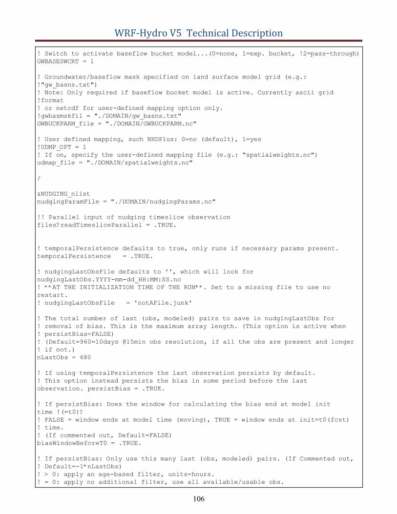
WRF-Hydro V5 Technical Description
! Switch to activate baseflow bucket model...(0=none, 1=exp. bucket, !2=pass-through)
GWBASESWCRT = 1
! Groundwater/baseflow mask specified on land surface model grid (e.g.:
!"gw_basns.txt")
! Note: Only required if baseflow bucket model is active. Currently ascii grid
!format
! or netcdf for user-defined mapping option only.
!gwbasmskfil = "./DOMAIN/gw_basns.txt"
GWBUCKPARM_file = "./DOMAIN/GWBUCKPARM.nc"
! User defined mapping, such NHDPlus: 0=no (default), 1=yes
!UDMP_OPT = 1
! If on, specify the user-defined mapping file (e.g.: "spatialweights.nc")
udmap_file = "./DOMAIN/spatialweights.nc"
/
&NUDGING_nlist
nudgingParamFile = "./DOMAIN/nudgingParams.nc"
!! Parallel input of nudging timeslice observation
files?readTimesliceParallel = .TRUE.
! temporalPersistence defaults to true, only runs if necessary params present. temporalPersistence = .TRUE.
! nudgingLastObsFile defaults to '', which will look for
nudgingLastObs.YYYY-mm-dd_HH:MM:SS.nc
! **AT THE INITIALIZATION TIME OF THE RUN**. Set to a missing file to use no restart.
! nudgingLastObsFile = 'notAFile.junk'
! The total number of last (obs, modeled) pairs to save in nudgingLastObs for
! removal of bias. This is the maximum array length. (This option is active when
! persistBias=FALSE)
! (Default=960=10days @15min obs resolution, if all the obs are present and longer
! if not.)
nLastObs = 480
! If using temporalPersistence the last observation persists by default.
! This option instead persists the bias in some period before the last
observation. persistBias = .TRUE.
! If persistBias: Does the window for calculating the bias end at model init
time !(=t0)?! FALSE = window ends at model time (moving), TRUE = window ends at init=t0(fcst)
! time.
! (If commented out, Default=FALSE)
biasWindowBeforeT0 = .TRUE.
! If persistBias: Only use this many last (obs, modeled) pairs. (If Commented out,
! Default=-1*nLastObs)
! > 0: apply an age-based filter, units=hours.
! = 0: apply no additional filter, use all available/usable obs.
106

WRF-Hydro V5 Technical Description
! < 0: apply an count-based filter, units=count
maxAgePairsBiasPersist = 24
! If persistBias: The minimum number of last (obs, modeled) pairs, with age less
!than
! maxAgePairsBiasPersist, required to apply a bias correction. (Default=8)
minNumPairsBiasPersist = 1
! If persistBias: give more weight to observations closer in time? (default=FALSE)
invDistTimeWeightBias = .TRUE.
! If persistBias: "No constructive interference in bias correction?", Reduce the
!bias adjustment
! when the model and the bias adjustment have the same sign relative to the modeled
!flow at t0?
! (default=FALSE)
noConstInterfBias = .TRUE.
/
107