South African Reserve Bank Working Paper Series

WP/2013/06

Important channels of transmission of monetary policy shock in South Africa

Nombulelo Gumata, Alain Kabundi and Eliphas Ndou

December 2013

ii

South African Reserve Bank Working Papers are written by staff members of the South African Reserve Bank and on occasion by consultants under the auspices of the Bank. The papers deal with topical issues and describe preliminary research findings, and develop new analytical or empirical approaches in their analyses. They are solely intended to elicit comments and stimulate debate. The views expressed in this Working Paper are those of the author(s) and do not necessarily represent those of the South African Reserve Bank or South African Reserve Bank policy. While every precaution is taken to ensure the accuracy of information, the South African Reserve Bank shall not be liable to any person for inaccurate information, omissions or opinions contained herein. South African Reserve Bank Working Papers are externally refereed. Information on South African Reserve Bank Working Papers can be found at http://www.resbank.co.za/Research/ResearchPapers/WorkingPapers/Pages/WorkingPapers-Home.aspx Enquiries Head: Research Department South African Reserve Bank P O Box 427 Pretoria 0001 Tel. no.: +27 12 313-3911

0861 12 SARB (0861 12 7272) © South African Reserve Bank All rights reserved. No part of this publication may be reproduced, stored in a retrieval system, or transmitted in any form or by any means without fully acknowledging the author(s) and this Working Paper as the source.

iii

Contents

Non-technical summary .................................................................................................................. v Abstract. ............................................................................................................................... 1 1. Introduction...................................................................................................................... 2 2. Large Bayesian Vector Autoregressive Model ................................................................ 5 3. Data and data transformation ......................................................................................... 8

4. Empirical Results………………………………………………………………………………………………………..9 4. Empirical Results………………………………………………………………………………………………………..9 4.1 Identification of Monetary Policy Shock ........................................................................... 9

4.2 Interest Rate Channel ..................................................................................................... 10

4.3 Asset Price Channel ........................................................................................................ 11

4.4 Expectation Channel ....................................................................................................... 11

4.5 Exchange Rate Channel .................................................................................................. 12

4.6 Lending Channel ............................................................................................................. 12

4.7 Balance Sheet Channel ................................................................................................... 14

4.8 Variance Decomposition ................................................................................................. 14 5. Conclusions………………………………………………………………………………………………………………16 References .......................................................................................................................... 18 Figures

1. Identification of Monetary Policy Shock ......................................................................... 22

2. Interest Rate Channel ..................................................................................................... 23

3. Asset Price Channel ........................................................................................................ 23

iv

4. Expectation Channel ....................................................................................................... 24

5. Exchange Rate Channel .................................................................................................. 24

6. Lending Channel ............................................................................................................. 25

7. Balance Sheet Channel ................................................................................................... 25 Tables

1. Variance Decomposition ................................................................................................. 22

2. Appendix: List of Variables and their treatments ........................................................... 26

v

Executive Summary

This paper investigates the importance of different channels of transmission of a monetary policy shock in South Africa. We apply a Large Bayesian Vector Autoregressive (LBVAR) model, which includes 165 quarterly variables observed from 2001Q1 to 2012Q2 to examine the effectiveness of a monetary policy shock based impulse response functions and variance decompositions. The panel contains nominal variables, real variables, and financial variables. The advantage of this empirical framework over the traditional Vector Autoregressive (VAR) models is that it can accommodate hundreds of variables and hence solving puzzling results observed in small VAR due to information deficiency. The framework we use in this study can identify all five channels of transmission of monetary policy in one setup. The channels studied are: the interest rate channel, the credit channel (lending and balance sheet), the asset price channel, exchange rate channel, and the expectations channel. The policy shock is measured by an unexpected 100 basis points increase in the repo rate. We rank the channels in descending order based on variance decompositions. The impulse response traces paths of variables in above mentioned channels to unexpected 100 basis points increase in repo rate. The results provide evidence that all five channels are working in South Africa. Real variables and nominal react negatively, and their impacts are statistically significant, but they do not last long. The exchange rate channel operates through trade. In addition, business confidence, consumer confidence, and inflation expectations decline with some lag and recover gradually. Balance sheets of banks are impaired following a contractionary monetary policy, showing the relevance of the lending channel. A negative monetary policy shock affects somewhat the ability of financial intermediaries in supplying loans to both corporates and households. The significant effects on household disposable income, total assets, and financial indicate that balance sheets are also operational in South Africa. The variance decomposition represents the proportion of movements of channels in response to unexpected 100 basis point increase in repo rate. The results, based on variance decomposition, show that the interest rate channel remains the most important channel of transmission of monetary policy in South Africa in the inflation-targeting regime. The lending channel is somewhat weak but it is more important than the balance sheet channel. It means that the contractionary monetary policy affects more the supply of loans than the demand for loans. Overall, the results point to fact that households are directly affected through the interest rate channel and the amplification of the shock work through other channels. The limited importance of the asset price channel can be attributed to a small portion of South African who hold share in the stock exchange. In addition, there are few people in the country who have mortgaged houses and use their houses as collateral to get more loans.

Important Channels of Transmission of Monetary

Policy Shock in South Africa�

Nombulelo Gumatay Alain Kabundiz Eliphas Ndoux

December 6, 2013

Abstract

This paper investigates the di¤erent channels of transmission of monetary pol-

icy shock in South Africa in a data-rich environment. The analysis contains 165

quarterly variables observed from 2001Q1 to 2012Q2. We use a Large Bayesian

Vector Autoregressive model, which can easily accommodate a large cross-section

of variables without running out of degree of freedom. The bene�t of this frame-

work is its ability to handle di¤erent channels of transmission of monetary policy

simultaneously, instead of using di¤erent models. The model includes �ve chan-

nels of transmission: credit, interest rate, asset prices, exchange rate, and expec-

tations. The results show that all channels seem potent, but their magnitudes and

importance di¤er. The results indicate that the interest rate channel is the most

important transmitter of the shock, followed by the exchange rate, expectations,

and credit channels. The asset price channel is somewhat weak.

JEL Classi�cation Numbers: C11, C13, C33, C53

Keywords: Bayesian VAR, Monetary policy transmission; Balance sheets, large

cross-sections

�Authors would like to thank Lucrezia Reichlin and participants of the ERSA monetary policy

conference. We also thank Domenico Giannone and Marta Banbura for assisting with their Matlab

codes.yResearch Department, South African Reserve Bank. Email: Nombulelo.Gumata@resbank.co.za.zResearch Department, Monetary Policy Unit, South African Reserve Bank,

Alain.Kabundi@resbank.co.za. Visiting Professor, Department of Economics, University of Jo-

hannesburg. Economic Research Southern Africa.xResearch Department, Monetary Policy Unit, South African Reserve Bank. Email:

Eliphas.Ndou@resbank.co.za.

1

1 Introduction

The monetary policy transmission mechanism has gained the attention of policymakers

and academics because it reveals the process through which central bank actions a¤ect

the real economy and in�ation. Boivin, Kiley, and Mishkin (2010) identify two basic

types of monetary transmission mechanism: neoclassical channels and non-neoclassical

channels. The traditional channels of monetary policy, also known as the neoclassical

channels, are based on the neoclassical models of investment proposed by Jorgenson

(1963) and Tobin (1969), the permanent income models of consumption developed by

Brumberg and Modigliani (1954), Ando and Modigliani (1963), and Friedman (1957),

and the ISLM models of Mundell (1963) and Fleming (1962).1 These channels assume

that �nancial markets operate in an environment of perfect information. The main

channel of transmission is the interest rate channel. According to this channel, an

expansionary monetary policy results in a decrease in the policy rate, which in turn

pushes the real interest rate down and hence the cost of capital decreases, investment

spending increases as a result, and ultimately aggregate demand increases, which causes

output to increase. The interest rate channel operates more through the real interest rate

than the nominal interest rate and the real long-term interest rate seems to have more

impact on spending that the short-term interest rate. Many researchers, for example

Taylor (1995), Boivin, Kiley, and Mishkin (2010), conclude that the interest rate channel

remains the most important channel for the transmission of monetary policy.

Besides the interest rate, other asset prices like equity prices, house prices, and the

exchange rate constitute non-negligible channels through which monetary policy a¤ects

the real economy. The exchange rate channel operates through international trade.

An expansionary monetary policy which decreases the short-term interest rate makes

domestic goods cheaper relative to foreign goods. Hence it causes the domestic currency

to depreciate, which in turn boosts exports relative to imports. The rise in net exports

translates directly into an increase in aggregate demand. Bryant, Hooper, and Mann

(1993), Taylor (1993), and Smets (1995) show evidence of the importance of this channel

in small and open economies with �exible exchange-rate regimes. Furthermore, the

exchange rate channel depends on the sensitivity of the exchange rate to changes in the

interest rate. By increasing investment and consumption, the expansionary monetary

policy causes upward movements in equity prices.2 The equity price channel also operates

via the value of businesses and housing. As the value of businesses and/or housing

increases relative to the cost of replacement, investment spending will rise, and this

1See Taylor (1995), Mishkin (1996), and Boivin, Kiley, and Mishkin (2010) for more details on the

review of literature on traditional channels of monetary policy.2Note that equity price refers to both stock price and house price.

2

triggers aggregate demand. The last traditional channel identi�ed in the literature is

the expectations channels. Central bank decisions about the future path of the short-

term rate a¤ect economic agents�views on the impact of central bank actions and its

reactions to various shocks that a¤ect the economy. The expectations of agents will

subsequently have an impact on their decisions to spend and invest �and hence will also

a¤ect output and price. However, agents�expectations are highly dependent on their

beliefs about the credibility of the central banks. If they believe that the central bank

is serious about in�ation, their expectations on the future price will be anchored around

the central bank in�ation targets. But if they think that the central bank accommodates

more output relative to price stability, their expectations about future price will not be

anchored.

The second type of transmission channel identi�ed by Boivin, Kiley, and Mishkin

(2010) is the non-neoclassical channel proposed by Bernanke and Gertler (1995), which

is commonly referred to as the credit channel.3 This channel is a result of frictions in

credit markets based on the asymmetry of information between lenders and borrowers.

It points to the important role played by �nancial intermediaries in the economy. It

becomes more important for small �rms and households who are highly dependent on

bank loans. There are two types of credit channel, namely, the bank lending channel

and the balance sheet channel. The �rst channel refers to the e¤ects of monetary policy

shock on the supply of loans by �nancial intermediaries, while the latter is concerned with

the demand for loans by �rms and households. The bank lending channel operates via

the external �nancial premium. Given the imperfect substitutability of bank deposits

and other sources of funds, a contractionary monetary policy increases the costs of

raising funds externally and the opportunity costs of funding internally, which in turn

a¤ects bank deposits and other sources of funds. Therefore it reduces the quantity of

bank loans available. Finally, the decline in quantity of loans reduces investment and

consumer spending, causing a fall in aggregate demand. Disyata (2011) argues that the

bank lending channel operates less through bank deposits and mainly via banks�balance

sheet strength and perceptions of risk. The second credit channel is the balance sheet

channel. A contractionary monetary policy increases debt service costs, which in turn

impairs assets and the collateral of households and �rms. These negative e¤ects on �rms�

balance sheets and the balance sheets of households undermine their creditworthiness.

The problem of asymmetrical information in debt �nancing, which arises from lower

net worth, induces a rise in external �nancial premium. The �nancial accelerator pushes

aggregate demand and output down even further. In contrast to the traditional channels,

there is less agreement in the literature on the relevance of the credit channel. While

3See these authors and references therein for more details.

3

Bernanke and Gertler (1995), Kiyotaki and Moore (1997), and Iacoviello (2005) o¤er

theoretical grounds for credit channel, Gertler and Gilchrist (1993 and 1994), Kashyap

and Stein (1995), Iacoviello and Minetti (2008), and Berger and Bouwman (2009) �nd

empirical evidence for the existence of this channel. On the other hand, Ramey (1993)

and Carlino and De�na (1998), and Fazylov, and Molyneux (2002) raise doubts about

the strength of this channel.

Besides Boivin, Kiley, and Mishikin (2010) and Igan et al. (2013), there are few

studies that include all �ve channels in one investigation. In addition, few empirical

studies investigate the relevance of both bank lending and the balance sheet channels of

monetary policy. Much research focuses on develop countries; the exception is Khun-

drakpam and Jain (2012), who examine the importance of these channels in India. The

current study bridges the existing gap in the literature by investigating the importance

of all �ve channels in South Africa within one framework, like Boivin et al. (2010) and

Igan et al. (2013). However, the framework adopted in this study di¤ers from the above

articles. Both Boivin et al. and Igan et al. use the Factor Augmented Vector Autore-

gressive (FAVAR) model, which can accommodate more than a hundred variables. But

this model induces the degree-of-freedom issue, which is common in standard VAR mod-

els. Given this, the current article uses the Large Bayesian VAR (LBVAR) proposed by

Banbura, Giannone, and Reichlin (2010, henceforth BGR) with Minnesota priors. The

LBVAR allows us to analyse the impact of contractionary monetary policy, in this case

a percentage rise in the policy rate, on any of the variables included in the dataset. In

addition, as in standard VAR, we use the variance decomposition to rank all six channels

according to their importance for the South African economy.

The current study is closely related to Kabundi and Ngwenya (2011), but the latter

considers the credit channel as a whole without including the bank lending channel

and the balance sheet channel separately. Breaking down the credit channel into bank

lending and balance sheet means that we have a total of six channels. Many studies on

channels of transmission of monetary policy in South Africa focus on the interest rate

channel of monetary policy. Brink and Kock (2010), in agreement with Disyatat (2011),

attest that the bank lending channel operates di¤erently. According to them banks are

not constrained by their deposits to supply loans. The supply of loans depends to a

large extent on the demand for loans, the a¤ordability of �rms and households, and the

risk-taking behaviour of banks.

We �nd that all six channels operate to a signi�cant degree in South Africa, but

that their e¤ects vary. As in Boivin et al. (2010), and unlike Khundrakpam and Jain

(2012), we �nd that the interest channel is by far the most important transmitter of

monetary policy shock. It is followed by the exchange rate. The important role played

4

by the exchange rate can be attributed to the fact that in a �oating exchange rate

regime the domestic currency becomes a shock absorber. The bank lending rate comes

in the third position. Monetary policy shock a¤ects bank deposits, the total equity

of banks, and claims on the domestic private sector alike. This means that monetary

policy shock a¤ects both the assets and liabilities of banks. The bank lending channel is

followed by the expectations channel, which is more evident in business and consumer

con�dence than in�ation expectations. In contrast to the balances of banks, the balances

of households have relatively small e¤ects. Finally, asset prices, both equity price and

house price, are the weakest channels through which monetary policy a¤ects the South

African economy.

The rest of the paper is organised as follows. Section 2 discusses the LBVARmethod-

ology. We describe the data and their transformations in Section 3. In Section 4 we

present the empirical results of all six channels of transmission of monetary policy using

the impulse response functions and the variance decomposition. Section 5 concludes the

paper with some policy recommendations.

2 Large Bayesian Vector Autoregressive Model

In recent empirical research in macroeconomics there has been an increasing trend of

using large-scale models that can contain hundreds of variables (Stock andWatson, 2002;

Forni, Hallin, Lippi, and Reichlin, 2000; Bernanke, Boivin, and Eliasz, 2005; Carriero,

Kapetanios and Marcellino, 2009; Banbura, Giannone, and Reichlin, 2010; Giannone,

Lenza, Momferatou and Onorante, 2010; Carriero, Clark and Marcellino, 2011; Koop,

2011; Koop and Korobilis, 2013). These models can be divided into two main categories:

those using factor analysis, which can accommodate large cross-sections of economic

variables, and the papers using the Large Bayesian Vector Autoregressive (LBVAR)

model, which deal with large number of time series through shrinkage of parameters.

The current study adopts the latter approach and follows closely the LBVAR proposed

by Banbura, Giannone, and Reichlin (2010; henceforth the BGR).4 BGR demonstrate

that the LBVAR leads to a better identi�cation of monetary policy shock. It solves

the problem of prize puzzle and output puzzle, which are common in small-scale VARs.

Hence, the LBVAR is an appropriate alternative to factor models.

Assume the VAR model of the form

Y = XB + U

where Y = (Y1; : : : ; YT )0 is a T�N matrix of dependent variables, X = (X1; : : : ; XT )

0 is a

4See BGR for more technical details of the LBVAR.

5

T �K matrix of explanatory variables, with Xt =�Y 0t�1; : : : ; Y

0t�p; 1

�0, U = (u1; : : : ; uT )

0

is a T �N matrix of error terms with ut being independent N (0;�), and B is a K �Nmatrix of coe¢ cients and K = (Np+ 1). A large VAR based on quarterly series with 50

variables and four lags contains over 10,000 parameters. With such a model it is possible

to obtain reliable estimate of parameters with higher precision, while many coe¢ cients

are statistically insigni�cant. This is known as the curse of dimensionality as large VAR

models have number of parameters increasing relative to number of observations. Hence,

impulse response functions are also imprecisely estimated. Recently, Stock and Watson

(2002), Forni, Hallin, Lippi, and Reichlin (2000), and Bernanke, Boivin, and Liasz (2005)

adopted the factor analysis framework to deal with the issue of proliferation parameters,

and they obtained good empirical results. Hence, they managed to turn the curse of

dimensionality into a blessing. On the other hand BGR, Koop (2011), and Koop and

Korobilis (2013) show that the blessing of dimensionality can be obtained using the

Bayesian approach through the shrinkage of coe¢ cients. The LBVAR imposes prior

beliefs on parameters as proposed by Doan, Litterman, and Sims (1984) and Litterman

(1986) and modi�ed by Kadiyala and Karlsson (1997), and Sims and Zha (1998).

The main issue in Bayesian analysis is the selection of proper priors, which leads

to a valid posterior distribution. This paper uses the prior beliefs suggested by Doan,

Litterman, and Sims (1984) and Litterman (1986), also known as Minnesota priors.

The principle is to shrink all equations around a random walk with a drift for variables

that show persistence and around white noise for variables that are mean-reverting. It

addresses the risk of over�tting the data, which is common in large models. This way

of shrinking coe¢ cients is simple and very attractive. Even though it is very restrictive

and that there are alternative ways of shrinking coe¢ cients in Bayesian VARs, Koop

(2011) �nds that the LBVAR based on Minnesota priors outperforms other LBVARs

based on stochastic variable selection (SSVS) when the cross-section gets larger.

Formally, we have:

Yt = c+ Yt�1 + ut (1)

Note that in Equation (2) all VAR coe¢ cients are shrunk towards zero, expect for

coe¢ cients of own and more recent lags of each dependent variable, which are set to

one. The rationale is that more recent lags provide more accurate information about

the variable than distant lags. In addition, own lags explain most of the variation in the

variable than the lags of other variables.

Equation (1) can be written as a V AR(p):

Yt = c+B1Yt�1 + � � �+BpYt�p + ut (2)

6

The Minnesota priors are set as:

E(Bk;i;j) =

(�i j = i, k = 1

0 otherwise

and V (Bk;i;j) =

(�2

k2j = i

�2�2

k2� �2i

�2jotherwise

(3)

Note that like in equation (3), the Minnesota prior set � to be one for all variables

that are nonstationary, while it is zero for all variables that are stationary. The error

matrix � = diag(�21; : : : ; �2N)is assumed to be diagonal, �xed and known.

The hyperparameter � speci�es the overall tightness of the prior distribution around

the random walk or white noise process. It expresses prior knowledge about the impor-

tance of the prior beliefs concerning the process that governs the data. � is set to zero

when the data does not in�uence the estimate and the posterior equals the prior. On

the other hand, when � is1, the posterior expectations coincide with the ordinary leastsquares (OLS) estimates. We choose � to avoid over�tting the model, which is common

in large models, such that parameters are shrunk even more. The 1=k2 re�ects the rate

of decay, which is a shrinkage of the variance with increasing lag length. The scaling

factor, �2i =�2j , adjusts for varying magnitudes of the variables across equations i and j.

The scalar �2�0 � �2 � 1

�is used for lags of less important variables with prior means

of zero and a decreasing variance as the lag length increases.

The restrictive assumption of �xed and diagonal covariance matrix, proposed by

Litterman (1986), makes it impossible to deal with the correlation among the residual

of di¤erent variables common in structural models. Kadiyala and Karlsson (1997) and

Robertson and Tallman modify the Minnesota prior and impose the inverted Wishart

prior. They set �2 = 1. The main issue with the Minnesota priors is that it assumes in

Equation (1) to be known and uses its estimate, �̂. For the VAR, the normal inverted

Wishart prior has the form:

� � N (�0;� ) and � � iW (�0; �) (4)

where � = vec(B) and �0, , �, and �0 are prior hyperparameters chosen such that

prior expectations of B coincide with the traditional Minnesota prior. Here the prior

and likelihood can be seen as coming from a �ctitious sample, as they have the same

distributional form. Like BGR we use a �ctitious sample of T0 dummy observations

Y0 and X0 to the Equation (1) such that = (X 00X0)

�1, �0 = (X 00X0)

�1X 00Y0, �0 =

(Y0 �X0�0)0 (Y0 �X0�0). According to Sims and Zha (1998), the dummy observation

approach is suitable for structural VARs. According to BGR, in order to have a prior

7

that coincides with the traditional Minnesota prior, the following �ctitious sample should

be added:

Y0 =

0B@ diag(�1�1; : : : ; �N�N)=�

0(Np�N+1)�N

diag(�1; : : : ; �N)

1CA X0 =

0B@ Jp diag(�1�1; : : : ; �N�N)=� 0Np�1

01�Np "

0N�Np 0N�1

1CA(5)

where Jp = diag(1; 2; : : : ; p), diag(�) denotes a diagonal matrix. As in BGR, the �rstblock of dummies set prior beliefs on the autoregressive coe¢ cients, the second block

uses the prior for the covariance matrix, and the last block represents the uninformative

prior for the intercept. Note that " is a very small number.

Putting together the original sample, T , and the �ctitious sample, T0, we obtain:

Y¯= X¯B +U

¯(6)

where T¯= T + T0, Y¯

= (Y 0; Y 00), X¯= (X 0; X 0

0), and U¯= (U 0; U 00). BGR show that adding

dummy observation serves as a solution to the matrix inversion problem and it helps in

imposing further restrictions.

3 Data and data transformation

The dataset contains 165 quarterly periods, including the real variables such as the

gross domestic product (GDP), gross �xed investment, �nal consumption expenditure;

nominal variables such as GDP de�ator, consumer price index, producer price index,

remuneration per worker; �nancial variables such as stock prices, real e¤ective exchange

rate, rand/dollar exchange rate, the repo rate, treasury bill, long-term interest rates;

and balance sheet variables from households and banks. The paper does not cover the

balance sheets of corporates due to lack of data during the period under investigation.

All series are logged, except those in percentages, the series with negative values, and

those containing zeros. The dataset covers a period ranging from 2001Q1 to 2012Q2.

The choice of the sample coincides with the in�ation-targeting regime in South Africa

that was implemented in 2000. We believe that it takes close to a year for the �rst e¤ects

of the new regime to become evident.

We use the Generalised Dickey-Fuller (DF-GLS) test, proposed by Elliot, Rothen-

berg, and Stock (1996), instead of the more popular Augmented Dickey-Fuller (ADF)

to assess the degree of integration of all series. This test does not have power and size

issues, which weaken the validity of results obtained using the ADF test. In addition, we

use the KPSS test proposed by Kwiatowski, Phillips, Schmidt, and Shin (1992), about

which we have no doubts. Unlike the DF-GLS, which assesses the presence of unit root

8

in series, the KPSS test uses the null hypothesis of stationary. Note that we do not

transform the series to induce stationarity; instead we use the Minnesota priors such

that �i = 1 for all nonstationary series and �i = 0 for series that are mean-reverting.

We choose � in such a way that the LBVAR model has the same �t as the VAR with

three variables (GDP, in�ation, and the repo rate) estimated with OLS. As in Bernanke,

Boivin, and Eiasz (2005), we divide the sample into two. Slow-moving variables are

those that react slowly to a monetary policy shock, such as real and nominal variables,

while fast-moving variables react contemporaneously to a monetary policy shocks, such

as �nancial variables.5 We use four lags in the VAR, which corresponds to a year. The

identi�cation procedure is such that slow-moving variables come �rst. These are fol-

lowed by the policy instrument, the repo rate, while fast-moving variables are ordered

last. We use 5,000 replications to construct impulse response functions (IRFs). The

posterior coverage of IRFs is set to 90% con�dence levels. In this analysis the monetary

policy shock increases the repo rate by 1% or 100 basis points.

4 Empirical Results

4.1 Identi�cation of Monetary Policy Shock

Figure 1 depicts the identi�cation of monetary policy which is correctly identi�ed, as

predicted by theory. The repo rate increases by 1% at impact and the e¤ects fade

away quickly in less than a year. The GDP reacts negatively, reaching the minimum

of 0.05% after a year. The impact of the shock lasts for closer to two years. Similarly,

in�ation decreases, but the e¤ect is short-lived. It is evident that the identi�cation

strategy we adopt solves the price puzzle, which is common in small VAR models, such

as Bonga-Bonga and Kabundi (2011). The price puzzle occurs when a rise in short-term

interest rate leads to an increase in in�ation instead of a decrease as predicted by theory.

Bernanke et al. (2005) and Banbura et al. (2010) argue that puzzling results obtained

in small VARs are the consequence of insu¢ cient information. The BGR show that a

model with 20 variables already solves puzzling results in real variables and prices. If

realistic information is not taken into account, it is more likely to mix structural shocks

and measurement errors. Furthermore, including more than 20 variables does not a¤ect

results negatively. Like GDP, the e¤ect on in�ation attains its peak of 0.12% after a

year and lasts for more than two years. These results point to long-term neutrality of

monetary policy. In response to contractionary monetary policy, personal consumption

expenditure (PCE) falls signi�cantly. In line with expectations, higher shorter-term

5See the Appendix for a description of the dataset.

9

interest rates make �nancing consumption through credit more expensive and in turn

compress growth in consumption expenditure in less than a year. However, the e¤ect on

consumption is somewhat less than the e¤ect on GDP and it is short-lived. It reaches

a minimum of 0.03% three quarters after the shock. But the e¤ect on the consumption

of durable goods is more pronounced and lasts longer. It declines by 0.13% after four

quarters and retreats to baseline level after a year and a half.

It is evident that contractionary monetary policy a¤ects real interest rates and long-

term interest rates, which in turn puts pressure on spending on durable goods and ulti-

mately depressing aggregate demand. Conventional analysis of monetary policy trans-

mission attributes strong reaction of consumption of durable goods to the fact that it

is the most interest-sensitive part of aggregate demand. The impact on growth in �xed

capital formation (GFCF growth) comes with a greater lag of three quarters. This is

consistent with the literature.6 Bernanke and Gertler (1995) explain the delay in reac-

tion by incredibly large adjustment costs. Businesses have a long-term perspective in

their investment decisions when faced with changes in interest rates. The short-term

interest rate elasticities of investment seem quite small.

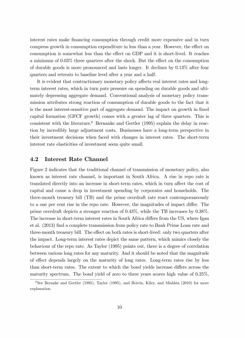
4.2 Interest Rate Channel

Figure 2 indicates that the traditional channel of transmission of monetary policy, also

known as interest rate channel, is important in South Africa. A rise in repo rate is

translated directly into an increase in short-term rates, which in turn a¤ect the cost of

capital and cause a drop in investment spending by corporates and households. The

three-month treasury bill (TB) and the prime overdraft rate react contemporaneously

to a one per cent rise in the repo rate. However, the magnitudes of impact di¤er. The

prime overdraft depicts a stronger reaction of 0.43%, while the TB increases by 0.38%.

The increase in short-term interest rates in South Africa di¤ers from the US, where Igan

et al. (2013) �nd a complete transmission from policy rate to Bank Prime Loan rate and

three-month treasury bill. The e¤ect on both rates is short-lived: only two quarters after

the impact. Long-term interest rates depict the same pattern, which mimics closely the

behaviour of the repo rate. As Taylor (1995) points out, there is a degree of correlation

between various long rates for any maturity. And it should be noted that the magnitude

of e¤ect depends largely on the maturity of long rates. Long-term rates rise by less

than short-term rates. The extent to which the bond yields increase di¤ers across the

maturity spectrum. The bond yield of zero to three years scores high value of 0.25%,

6See Beranke and Gertler (1995), Taylor (1995), and Boivin, Kiley, and Mishkin (2010) for more

explanation.

10

while the 10-year bond has a relatively weak response of 0.06%. As with short-term

rates, the e¤ect has the same duration as the policy rate, i.e. two quarters.

4.3 Asset Price Channel

Besides stock, assets include real estate assets, in this case housing. The asset price

channel is closely related to the consumption channel, also known as the wealth channel.

A rise in the short-term rate a¤ects demand for stock negatively and consequently stock

prices drop. The all-share index (JSE) does not react upon impact, and eventually

decreases gradually, attaining the lowest level of 0.32% after two quarters (see Figure 3).

The decline is consistent with Kabundi and Ngwenya�s (2011) �ndings. The magnitude of

decline is relatively high in comparison to the e¤ect on house prices. House prices do not

react contemporaneously, but the e¤ect is statistically signi�cant, reaching a minimum

value of 0.08% after two quarters. In contrast to Kasai and Gupta (2008), who �nd

evidence of the home price puzzle, the result is in line with theory.7 In addition, an

increase in the repo rate curtails demand for housing and hence residential investment

declines. Residential investment decreases sharply, but the e¤ect is contained in the

short run. Bernanke and Gertler (1995) observe that the e¤ect of monetary policy

on residential investment is larger than the e¤ect on private investment. In contrast

to a lag and small reaction of GFCF growth, reaching its lowest level of 0.06% after

four quarters, residential investment reacts faster and attains the minimum of 0.15%.

Moreover, a positive monetary policy shock impairs the net wealth of households.

4.4 Expectation Channel

Business con�dence and consumer con�dence levels are closely related to the �ndings

by Kabundi and Ngwenya (2011), even though the magnitude and time of e¤ects di¤er

somewhat. More importantly, the missing variable in Kabundi and Ngwenya (2011) is

in�ation expectations, which play an essential part in the expectation channel of mon-

etary policy. In Figure 4 we can observe that business con�dence (BERBCI) contracts

more than consumer con�dence (CCI). It indicates that the perception of agents is that a

contractionary monetary policy a¤ects business more than consumers. BER BCI attains

a maximum decline of 0.61% after two quarters and the e¤ects vanish gradually. The

e¤ect on consumer con�dence is short-lived and reaches the maximum decline of 0.15%

at the same time. The reactions of both business con�dence and consumer con�dence7Gupta, Jurgilas, and Kabundi (2010) �nd that the home price puzzle observed in Kasai and Gupta

(2008) is due to information de�ciency in small VAR models. They solve the puzzle with a FAVAR

model containing 246 variables.

11

lead real variables (GDP, PCE, and PCE Durable) by approximately two quarters. This

is essential for the conduct of monetary policy, especially in in�ation-targeting regime.

Monetary policy authority aims at anchoring expectations of economic agents. It seems

the SARB has been successful when it comes to the e¤ects of the policy on the real

economy.

However, the outcome is di¤erent concerning the expectations about in�ation. In�a-

tion expectations increase and stay positive for about a year and then become neg-

ative, and �nally die out gradually. The reaction of in�ation expectation may be

due to backward-looking expectation formation of market participants in South Africa.

Kabundi and Schaling (2013) attribute this behaviour to the fact that the implicit in-

�ation target is higher that the o¢ cial in�ation target.8 In addition, they �nd that the

weight allocated to output deviation from its full potential is higher than the weight

allocated to in�ation deviation from its target.

4.5 Exchange Rate Channel

Boivin et al. (2010) argue that the strength of the exchange rate channel in the monetary

policy transmission depends on two main factors. Firstly, the exchange rate is sensitive

to changes in interest rate. The exchange rate channel is potent when the exchange rate

is very sensitive to interest rate movements, as in the case of uncovered interest rate

parity. Secondly, the channel seems larger in open economies. Figure 5 shows that the

real e¤ective exchange rate reacts immediately upon impact and increases slightly and

becomes signi�cant and stays high for eight quarters, and then becomes insigni�cant.

However, the rise in interest rate does not translate into the in�ow of funds into South

Africa, seeking a high yield, but it does stop funds from leaving the country. Capital

out�ows drop; nevertheless, the decline is short-lived. The appreciation of the domestic

currency puts pressure on exports, which decline temporarily. The negative impact on

exports pushes aggregate demand down even further. The impact on the current account

is delayed by about a year and then improves for about a year.

4.6 Lending Channel

The lending channel of monetary policy, as one of the non-neoclassical channels, also

known as the credit channel, is based on market imperfections. These imperfections

are the consequences of asymmetrical information between lenders and borrowers.9 The

8Kabundi and Schaling (2013) estimate the implicit in�ation target to be 6.7%, which is consistent

with Klein (2012), while the midpoint of the target range is 4.5%.9Bernanke and Gertler (1995) for more details on credit channels.

12

lending channel refers to the e¤ects monetary policy has on the supply of loans to both

households and �rms. Mortgage advances, money supply M3, and total credit extended

to private sector deal with both supply and demand for loans. Unlike Kabundi and

Ngwenya (2011), who discuss the credit channel as a whole, this paper distinguishes

between the lending channel and balance sheet channel of monetary policy, and analyses

these two components of the credit channel separately.

It is clear from Figure 6 that a percentage increase in the repo rate decreases mort-

gage advances, total loans and advances, the credit extended to private sector, and the

money supply (M3) by almost the same magnitude, except for credit to the private

sector, which registers a considerable decline of 0.12%. The decline in total loans and

advances becomes signi�cant four quarters after the shock and lasts until the tenth quar-

ter. Similarly, total credit to private sector declines between six and ten quarters. Bank

balance sheets are impaired. Equity and liability of banks increase shortly after the

impact and then decrease and reach the minimum two years after the shock and then

the e¤ects die out gradually. It is evident that contractionary monetary policy to some

extent a¤ects the ability of the �nancial intermediary to supply loans to both corporates

and households. It is even clear when we consider the separately equity and deposits.

Total equity drops immediately upon impact and attains the minimum of 0.21% after

three quarters, while total deposits decrease gradually, reaching the minimum �ve quar-

ters after the shock. Furthermore, the asset side of the balance sheets of banks is a¤ected

even more than the liability side. As Disyatat (2011) suggests, the bank lending channel

a¤ects the demand for loans more. Total claims on the private sector decrease gradually

and attain a minimum of 0.12% �ve quarters after the shock.

Moreover, the ratio of deposits to liability shows an important decline right after the

shock, but it recovers quickly. Consequently, �nancial institutions record a rise of non-

performing loans (NPLs), attaining a maximum of 0.17% after three quarters due to the

inability of households and �rms to pay back loans. In addition, �nancial intermediaries

deleverage quickly following an increase in short-term rates. The ratio of total equity

and liability to total liability shrinks, indicating the negative e¤ects of monetary policy

on the size of the balance sheets of banks. In this environment banks become risk averse.

This implies that contractionary monetary policy reduces the risk-taking behaviour of

banks, which is common in lower interest rate regimes. The realised volatility of monthly

returns on bank stocks, as a measure of overall risk to banks, decreases sharply upon

impact. Finally, interest received as a percentage of credit extended to the private sector

and interest paid as a share of total deposits both increase.

13

4.7 Balance Sheet Channel

There is also evidence that monetary policy a¤ects households through the household

balance channel. This channel accounts for the e¤ects of monetary policy on the demand

for loans. Given the lack of information on the balance sheets of �rms, the analysis fo-

cuses on the balance sheets of households. Household disposable income falls signi�cantly

for nearly two years. At the peak e¤ects of a monetary policy shock, disposable income

falls by nearly 0.08% in the third quarter. Household total assets fall signi�cantly, and

the impact lasts for about a year. The decline in �xed assets follows the same pattern

as that of total assets. It reaches the maximum value of 0.09% three quarters after

the shock and recovers quickly. The combination of lower net wealth and the negative

e¤ects of household assets push up the external �nancial premium to 0.1%, which stays

up for three quarters. Because the balance sheets of households are impaired, the cost

of raising funds externally increases.

The household�s liability side, which comprises loans, is highly responsive to a mone-

tary policy shock. The liabilities of households remain depressed for two years, which is

double the period experienced by households�assets. Debt servicing costs rise by 0.85%

on impact, with the e¤ects dissipating within a year. In addition, total household debt

contracts for two years. In addition we �nd that the prime overdraft rate increases by

0.43% on impact, which is less than the increase in repo rate.

4.8 Variance Decomposition

Table 1 depicts the variance decomposition, which in turn indicates the importance of

analysing the di¤erent channels of monetary policy shock. It is clear from the table

that the interest rate channel seems the most potent. This accords with the views of

Boivin et al. and Bernanke and Gertler (1995). Short-term interest rates, represented by

prime overdraft and the three-month treasury bill, score the highest values of variance

decomposition. They are followed by long-term interest rates of di¤erent maturities. It

is evident that the traditional channel of transmission of monetary policy is still the

most important channel in South Africa, post the in�ation-targeting era. It is essential

to note that short-term rates translate directly into interest received and interest paid by

banks, which in turn a¤ect the balance sheet of banks. Similarly, changes in short-term

interest rates induce movements in debt servicing costs, which a¤ect the balance sheets

of households, and therefore the demand for loans. They also directly a¤ect the external

�nancial premium, which subsequently a¤ects the balance sheets of households.

The second most important channel is the exchange rate channel. As correctly

pointed out by Boivin et al. (2010), this channel seems to be large in small, open

14

economies, like South Africa. Since the adoption of the in�ation-targeting policy, the

country adopted a �oating exchange rate, which has become a non-negligible channel of

transmission of various shocks. With the variance decomposition of 0.58%, the exchange

rate channel is weak relative to the interest rate channel. Similar to the results obtained

from the IRFs, the exchange rate channel seems to transmit more via capital out�ows,

exports, and imports than through capital in�ows. A rise in the repo rate does not

translate into massive capital in�ows; instead, it stops capital from leaving the country.

The lending channel is the third most important in South Africa. Along the same

lines as the exchange rate channel, the lending channel depicts a variance decomposition

of 0.39% for deposits to liability ratio, which is somewhat weak. The percentage of

equity and liability as a share of total liability scores a variance decomposition of 0.13%.

It is evident from this analysis that the lending channel is more important than the

balance sheet channel. Thus a contractionary monetary policy a¤ects the supply of loans

more than it does the demand for loans. Even though the balance sheets of households

are impaired the impacts are not comparable to those of �nancial intermediaries. The

variance decomposition of household disposable income, �nancial liabilities, and debts

are 0.23%, 0.20%, and 0.18% respectively. Household total assets and household equity

and investment funds show very low values of variance decomposition of (0.08% and

0.04% respectively). The results point to the fact that households are directly a¤ected

through the interest rate channel and the ampli�cation of the shock through their balance

sheets is rather weak. The story would have been di¤erent had the analysis included the

balance sheets of corporates.

The expectation channel is the fourth most important channel after the interest

rate, the exchange rate, and the lending channel. The variance decomposition portrays

the same picture observed with the IRFs. Business con�dence is the most important

channel when it comes to expectation, with a variance decomposition of 0.29% compared

to 0.16% for consumer con�dence. Even though in�ation expectations depict a higher

value of variance decomposition, 0.87%, Figure 4 shows they mainly lag behind business

con�dence and consumer con�dence.

Finally, the asset price channel is outweighed by all the other channels. They have

the lowest values of variance decomposition �0.13% for house price, 0.12% for JSE, and

0.07% for household net wealth. The relative unimportance of the asset price channel

can be attributed to the fact that only a small proportion of South Africans hold shares

on the stock exchange. In addition, there are few people in the country who use their

houses as collateral to get more loans.

15

5 Conclusions

This paper analyses the importance of the six channels of transmission of monetary

policy in South Africa after the institution of the in�ation-targeting regime. Besides

the neoclassical channel of transmission of monetary policy, the analysis includes the

non-neoclassical channels proposed by Bernanke and Gertler (1995). The empirical

framework consists of the large Bayesian vector autoregressive (VAR) model of Banbura

et al. (2010), which contains 162 quarterly variables, including the real variables, nom-

inal variables, �nancial variables, and balance sheet variables of households and banks.

The dataset covers a period ranging from 2001Q1 to 2012Q2.

The results from impulse responses indicate that all channels are relevant in South

Africa. The interest channels are the most important. Short- and long-term interest rates

react quickly upon impact and are forcefully transmitted to real and nominal variables.

GDP, consumption expenditure and investment drop and recover slowly. Similarly, prices

decline, but the impact is not permanent. The data-rich environment solves the puzzling

results observed in most small-scale VAR models. Asset price prices, both stock prices

and house prices, are a¤ected by contractionary monetary policy. Importantly, the

policy during the in�ation-targeting regime a¤ects expectations about the real economy

more, but does not anchor price expectations. In�ation expectations lag considerably.

Like most open economies, the exchange rate channel seems a somewhat important

transmitter of monetary policy. It operates more via capital out�ows and trade than

through capital in�ows. In addition, the paper �nds evidence that non-neoclassical

channels are essential transmitters of monetary policy. The balance sheets of banks and

households alike are a¤ected, hence impairing the supply of and demand for loans. A

rise in the external �nancial premium due to the worse state of the balance sheets of

households further a¤ects the supply of loans to households. Although the paper does

not comprehensively address the risk-taking channel of monetary policy, the results show

that the ratio of deposits to liability shows an important decline right after the shock;

consequently, �nancial institutions record a rise of non-performing loans (NPLs). In

addition, �nancial intermediaries deleverage quickly following an increase in short-term

rates. The ratio of total equity and liabilities to total liabilities shrinks, indicating the

negative e¤ects of monetary policy on the size of the balance sheet of banks. In this

environment banks become risk averse. This implies that a contractionary monetary

policy reduces risk-taking behaviour of banks, which is common in lower interest rate

regimes. The realised volatility of monthly returns on bank stocks, as a measure of bank

overall risk, decreases sharply at impact.

The results obtained from variance decomposition point to the superiority of the

interest rate channel of monetary policy over the other �ve channels. The new policy

16

regime, in�ation-rate targeting, which advocates a �oating exchange rate, makes the

latter a shock absorber. Exchange rate has become a transmitter of various shocks,

including monetary policy shocks. The third important channel is the lending channel,

followed by the expectation channel. Unlike the balance sheets of banks, the balance

sheets of households do not play a major role in transmitting monetary policy shocks

to the economy. Finally, asset prices secure the last position among the six channels

included in this study.

17

References

[1] Ando, A. and F. Modigliani, 1963, �The "Life Cycle" Hypothesis of Saving: Ag-

gregate Implications and Tests,�American Economic Review, 53 (1), March, pp.

55�84.

[2] Banbura, M., D. Giannone, and L. Reichlin, 2010, �Large Bayesian Vector Auto

Regression,�Journal of Applied Econometrics, 25, pp. pp. 71�92.

[3] Bernanke, B. and M. Gertler, 1995, �Inside the Black Box: The Credit Channel

of Monetary Policy Transmission,� Journal of Economic Perspectives, 9 (4), pp.

27�48.

[4] Berger, A.N. and C.H.S. Bouwman, 2009, �Bank Liquidity Creation,�Review of

Financial Studies, 22 (9), pp. 3779�837.

[5] Bernanke, B. S., J. Boivin, and P. Eliasz, 2005, �Measuring the E¤ects of Monetary

Policy: A Factor-Augmented Vector Autoregressive (FAVAR) Approach,�Quarterly

Journal of Economics, 120 (1), February, pp. 387�422.

[6] Boivin, J., M. T. Kiley, and F. S. Mishkin, 2010, �How Has the Monetary Trans-

mission Mechanism Evolved Over Time?�NBER Working Paper No. 15879.

[7] Brink, N and M. Kock. 2010. �Central bank balance sheet policy in South Africa

and its implications for money-market liquidity,�SARB Working Paper 10/01.

[8] Brumberg, R. E. and F. Modigliani, 1954, �Utility Analysis and the Consumption

Function: An Interpretation of Cross-section Data,�in Post-Keynesian Economics,

ed. by K. Kurihara (New Brunswick, New Jersey: Rutgers University Press).

[9] Bryant, R., P. Hooper, and C. Mann 1993. "Evaluating Policy Regimes: New Em-

pirical Research in Empirical Economics." Washington, D.C., Brookings Institution.

[10] Carlino, G. and R. De�na, 1998, �The Di¤erential Regional E¤ects of Monetary

Policy,�Review of Economics and Statistics, 80 (4), November, pp. 572�87.

[11] Carriero, A., Clark, T. and Marcellino, M. (2011). �Bayesian VARs: Speci�cation

choices and forecast accuracy,�Federal Reserve Bank of Cleveland, working paper

11-12.

[12] Carriero, A., Kapetanios, G. andMarcellino, M. (2009). �Forecasting exchange rates

with a large Bayesian VAR,�International Journal of Forecasting, 25, 400-417.

18

[13] Doan, T., Litterman, R. and Sims, C. (1984). �Forecasting and conditional projec-

tions using a realistic prior distribution,�Econometric Reviews, 3, 1-100.

[14] Disyatat, P. 2011. �The Bank Lending Channel Revisited,� Journal of Credit,

Money, and Banking, 43(4): 711 �734.

[15] Elliott, G., T. J. Rothenberg, and J. Stock, 1996, �E¢ cient Tests for an Autore-

gressive Unit Root,�Econometrica, 64, pp. 813�36.

[16] Fleming, J. M., 1962, �Domestic Financial Policies under Fixed and under Floating

Exchange Rates,�IMF Sta¤ Papers, 9 (3), November, pp. 369�80.

[17] Forni M, Hallin M, Lippi M, Reichlin L. 2000. �The generalized dynamic factor

model: identi�cation and estimation,�Review of Economics and Statistics, 82: 540�

554.

[18] Friedman, M., 1957, �A Theory of the Consumption Function,�NBER Books No.

57-1, September.

[19] Gertler, M. and S. Gilchrist, 1993, �The Role of Credit Market Imperfections in

the Monetary Transmission Mechanism: Arguments and Evidence,�Scandinavian

Journal of Economics, 95 (1), pp. 43�64.

[20] Gertler, M. and S. Gilchrist, 1994, �Monetary Policy, Business Cycles and the

Behavior of Small Manufacturing Firms,�Quarterly Journal of Economics, 109,

pp. 309�40.

[21] Giannone, D., M. Lenza, and L. Onorante, 2010, �Short-term In�ation Projections:

A Bayesian Vector Autoregressive Approach,�forthcoming in International Journal

of Forecasting.

[22] Gupta, R., M.Jurgilas, and A. Kabundi, 2010, �The E¤ect of Monetary Policy on

Real House Price Growth in South Africa: A Factor Augmented Vector Autoregres-

sive (FAVAR) Approach,�Economic Modelling, 27: 315-323.

[23] Igan, D., A. Kabundi, F. Nadal De Simone, and N. Tamirisa 2013, �Monetary

Policy and Balance Sheets,�IMF Working Paper 13/158.

[24] Iacoviello, M., 2005, �House Prices, Borrowing Constraints, and Monetary Policy

in the Business Cycle,�American Economic Review, 95 (3), June, pp. 739�64.

19

[25] Iacoviello, M. and R. Minetti, 2008, �The Credit Channel of Monetary Policy:

Evidence from the Housing Market,� Journal of Macroeconomics, 30 (1), March,

pp. 69�96.

[26] Jorgenson, D., 1963, �Capital Theory and Investment Behavior,�American Eco-

nomic Review, 53 (2), May, pp. 247�59.

[27] Kabundi, A. and E. Schaling, 2013, �In�ation and In�ation Expectations in South

Africa: An Attempt at Explanation,�South African Journal of Economics, 81(3):

346-355.

[28] Kabundi, A. and L. Bonga-Bonga 2011, �Monetary Policy Action and In�ation in

South Africa: An Empirical Analysis,�African Finance Journal, 13(2): 25-37.

[29] Kabundi, A. and N. Ngwenya, 2011, �Assessing Monetary Policy in South Africa

in a Data-rich Environment,�South African Journal of Economics, 79(1): 91-107.

[30] Kadiyala KR, Karlsson S, 1997, �Numerical methods for estimation and inference

in Bayesian VAR-models,�Journal of Applied Econometrics 12(2): 99�132.

[31] Kasai, N, Gupta, R., 2008, �Financial Liberalization and the E¤ectiveness of Mone-

tary Policy on House Prices in South Africa,�Department of Economics, University

of Pretoria. Working Paper No. 200803.

[32] Kashyap, A. K. and J. C. Stein, 1995, �The Impact of Monetary Policy on Bank

Balance Sheets,�Carnegie-Rochester Conference Series on Public Policy, 42 (1),

June, pp. 151�95.

[33] Khundrakpam, J.K and Jain, R 2012. �Monetary Policy Transmission in India: A

Peep Inside the Black Box,�RNI Working Paper 11/2012

[34] Kiyotaki, N. and J. Moore, 1997, �Credit Cycles,�Journal of Political Economy,

105 (2), pp. 211�48.

[35] Klein, N. 2012, �Estimating the Implicit In�ation Target of the South African

Reserve Bank,�IMF Working Paper 12/177.

[36] Koop, G. and Korobilis, D. (2013). �Large Time-Varying Parameter VARs�, forth-

coming in Journal of Econometrics.

[37] Kwiatkowski, D., P. Phillips, P. Schmidt, and Y. Shin, 1992, �Testing the Null

Hypothesis of Stationarity Against the Alternative of a Unit Root: How Sure Are

20

We That Economic Time Series Have a Unit Root?�Journal of Econometrics, 54,

pp. 159�78.

[38] Litterman, R. (1986), "Forecasting with Bayesian vector autoregressions - Five years

of experience". Journal of Business and Economic Statistics 4, 25�38.

[39] Mishkin, F. S., 1996, �The Channels of Monetary Transmission: Lessons for Mon-

etary Policy,�NBER Working Paper No. 5464.

[40] Mundell, R.A., 1963, �Capital Mobility and Stabilization Policy under Fixed and

Flexible Exchange Rates,�Canadian Journal of Economics, 29, pp. 475�85.

[41] Ramey, V. A., 1993, �How Important is the Credit Channel in the Transmission of

Monetary Policy?�NBER Working Paper No. 4285.

[42] Sims CA and Zha T. 1998. �Bayesian methods for dynamic multivariate models,�

International Economic Review, 39(4): 949�968.

[43] Smets, F, 1995, �Central bank macroeconometric models and the monetary policy

transmission mechanism�, in: BIS (1995), Financial structure and the monetary

policy transmission mechanism, C.B. 394, March.

[44] Stock JH, Watson MW, 2002a, �Forecasting using principal components from a

large number of predictors,� Journal of the American Statistical Association, 97:

1167�1179.

[45] Taylor, John B., 1993. Macroeconomic Policy in a World Economy: From Econo-

metric Design to Practical Operation, W.W. Norton, New York.

[46] Taylor, JB, 1995, �The Monetary Transmission Mechanism: An Empirical Frame-

work,�Journal of Economic Perspectives, 9(4): 11-26.

[47] Tobin, J., 1969, �A General Equilibrium Approach to Monetary Theory,�Journal

of Money, Credit, and Banking, 1 (1), February, pp. 15�29.

21

Rank Series VD Rank Series VD Rank Series VD

1 Prime overdraft rate 18.475 16 Inflation 0.553 31 Equity and Liability 0.129

2 Treasury Bill 16.851 17 Deposits to liabilities 0.391 32 House Price 0.125

3 Received banks % of claims 13.778 18 GFCF Residential buildings 0.366 33 JSE 0.117

4 Paid banks % of deposits 13.399 19 BER Business Confidence 0.285 34 FCE Durable 0.110

5 Yield 0 to 3 years 7.766 20 GFCF growth 0.275 35 Exports 0.099

6 Yield 3 to 5 years 6.871 21 HH diposable income 0.233 36 Imports 0.097

7 Yield 5 to 10 years 3.178 22 HH Financial liabilities: Loans 0.200 37 Household assets 0.085

8 Financial leverage 2.456 23 Total HH debt 0.180 38 Current Account 0.074

9 External Financial Premium 2.427 24 PCE 0.171 39 Household net wealth 0.073

10 Debt service costs 2.303 25 BER Consumer Confidence 0.157 40 M3 0.054

11 Yield 10 years and more 1.071 26 Total credit to private sector 0.155 41 HH Equity & investment fund 0.042

12 Inflation Expectations 0.866 27 Total loans and advances 0.145 42 NPLs 0.031

13 GDP 0.829 28 Mortgage advances 0.145 43 Capital in 0.002

14 Bank risk 0.780 29 HH Fixed assets 0.142

15 REER 0.579 30 Capital out 0.136

Table 1: Variance Decomposition

Figure 1 Identi�cation of Monetary Policy Shock

0 4 8 12 16 20 24­0.08

­0.06

­0.04

­0.02

0

0.02

0.04

0.06

GDP

0 4 8 12 16 20 24­0.15

­0.1

­0.05

0

0.05

0.1

0.15

0.2GFCF growth

0 4 8 12 16 20 24­0.1

­0.05

0

0.05

0.1

0.15PCE

0 4 8 12 16 20 24

­0.4

­0.2

0

0.2

0.4FCE Durable

0 4 8 12 16 20 24­0.2

­0.15

­0.1

­0.05

0

0.05

0.1

0.15Inflation

0 4 8 12 16 20 24­0.2

0

0.2

0.4

0.6

0.8

1

REPO

22

Figure 2 Interest Rate Channel

0 4 8 12 16 20 24­0.05

0

0.05

0.1

0.15

0.2

0.25

0.3

Yield 0 to 3

0 4 8 12 16 20 24­0.02

0

0.02

0.04

0.06

0.08

0.1Yield 10 and more

0 4 8 12 16 20 24

0

0.1

0.2

0.3

0.4

TB

0 4 8 12 16 20 24­0.1

0

0.1

0.2

0.3

0.4

0.5

0.6Prime overdraft rate

Figure 3 Asset Price Channel

0 4 8 12 16 20 24

­0.4

­0.2

0

0.2

0.4GFCF Resid build

0 4 8 12 16 20 24­0.8

­0.6

­0.4

­0.2

0

0.2

0.4

0.6

JSE

0 4 8 12 16 20 24­0.15

­0.1

­0.05

0

0.05

0.1

0.15

0.2

HP

0 4 8 12 16 20 24­0.3

­0.2

­0.1

0

0.1

0.2

0.3

0.4Household net wealth

23

Figure 4 Expectation Channel

0 4 8 12 16 20 24­1

­0.8

­0.6

­0.4

­0.2

0

0.2

0.4

0.6

0.8BER BCI

0 4 8 12 16 20 24­0.4

­0.3

­0.2

­0.1

0

0.1

0.2

0.3CCI

0 4 8 12 16 20 24­0.06

­0.04

­0.02

0

0.02

0.04

0.06

0.08

0.1

0.12Inflation Expectations

Figure 5 Exchange Rate Channel

0 4 8 12 16 20 24

­1000

­500

0

Capital out

0 4 8 12 16 20 24­300

­200

­100

0

100

200

300Capital in

0 4 8 12 16 20 24­0.6

­0.4

­0.2

0

0.2

0.4

0.6

0.8Exports

0 4 8 12 16 20 24­0.8

­0.6

­0.4

­0.2

0

0.2

0.4

0.6

Imports

0 4 8 12 16 20 24­1500

­1000

­500

0

500

1000Current Account

0 4 8 12 16 20 24­0.5

0

0.5

1REER

24

Figure 6 Lending Channel

0 4 8 12 16 20 24­0.2

­0.1

0

0.1

0.2

Mortgage advances

0 4 8 12 16 20 24­0.2

­0.1

0

0.1

0.2

Total loans and advances

0 4 8 12 16 20 24­0.4

­0.2

0

0.2

0.4Total credit to priv

0 4 8 12 16 20 24­0.5

0

0.5

1short and med term deps

0 4 8 12 16 20 24­0.2

­0.1

0

0.1

0.2

M3

0 4 8 12 16 20 24­0.4

­0.2

0

0.2

0.4

EQuity and Liability

0 4 8 12 16 20 24­0.15

­0.1

­0.05

0

0.05

Deposits to liabilities

0 4 8 12 16 20 24­1

­0.5

0

0.5

1NPLs

0 4 8 12 16 20 24­1

­0.5

0

0.5

1Total equity

0 4 8 12 16 20 24­0.2

­0.1

0

0.1

0.2

Total deposits

0 4 8 12 16 20 24­0.4

­0.2

0

0.2

0.4Claims on private sector

0 4 8 12 16 20 24­0.3

­0.2

­0.1

0

0.1Financial leverage

0 4 8 12 16 20 24­0.05

0

0.05

0.1

0.15 Received  % of claims

0 4 8 12 16 20 24

0

0.05

0.1 Paid  % of deposits

0 4 8 12 16 20 24

­2

­1

0

Bank Risk

Figure 7 Balance Sheet Channel

0 4 8 12 16 20 24­0.15

­0.1

­0.05

0

0.05

0.1

0.15

0.2

HH Fixed assets

0 4 8 12 16 20 24­0.8

­0.6

­0.4

­0.2

0

0.2

0.4

0.6

HH Equity & inv fund

0 4 8 12 16 20 24­0.2

­0.1

0

0.1

0.2

HH Fin liabilities: Loans

0 4 8 12 16 20 24­0.2

­0.1

0

0.1

0.2Total HH debt

0 4 8 12 16 20 24­0.2

­0.15

­0.1

­0.05

0

0.05

0.1

0.15HH disposable income

0 4 8 12 16 20 24­0.4

­0.3

­0.2

­0.1

0

0.1

0.2

0.3Household assets

0 4 8 12 16 20 24

0

0.5

1

1.5

Debt serv costs

0 4 8 12 16 20 24

0

0.05

0.1

EFP

25

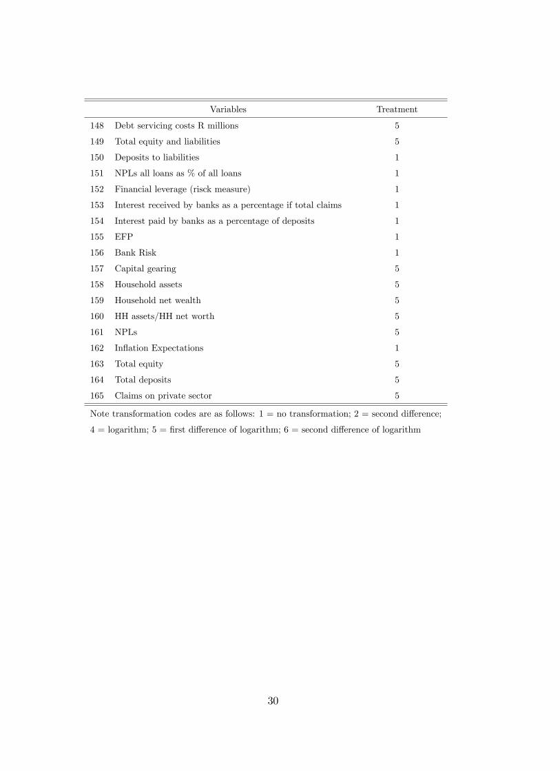
Appendix: List of Variables and their treatments

Variables Treatment

1 GDP 5

2 Employment Total Public sector 5

3 Employment National departments 5

4 Employment Provinces 5

5 Employment Total Private sector 4

6 Employment Total Mining 5

7 Employment Gold mining 5

8 Employment Non gold mining 5

9 Employment Manufacturing 5

10 Employment Construction 5

11 Remuneration per worker in the non-agricultural sector: Public sector, real 5

12 Remuneration per worker in the non-agricultural sector: Private sector, real 5

13 Total remuneration per worker in the non-agricultural sector, real 5

14 Labour productivity in the non-agricultural sectors 5

15 Nominal unit labour costs in the non-agricultural sectors 5

16 Gross national income (GNI) 5

17 Gross saving - Total 5

18 Net saving by general government 1

19 Compensation of residents 5

20 Disposable income of households 5

21 Savings by households 1

22 Gross �xed capital formation: Residential buildings - Total (Investment) 5

23 Gross �xed capital formation: Non-residential buildings - Total (Investment) 5

24 Gross �xed capital formation: Construction works - Total (Investment) 5

25 Gross �xed capital formation: Transport equipment - Total (Investment) 5

26 Gross �xed capital formation: Mining and Quarrying (Investment) 5

27 Gross �xed capital formation: Manufacturing (Investment) 5

28 Gross �xed capital formation: Electricity, gas and water (Investment) 5

29 Gross �xed capital formation (Investment) 5

30 Gross �xed capital formation: General government (Investment) 5

31 Gross �xed capital formation: Private business enterprises (Investment) 5

32 Final consumption expenditure by households: Total (PCE) 5

33 Final consumption expenditure by general government 5

34 Change in inventories 2

35 Final consumption expenditure by households: Durable goods 5

36 De�ator Gross domestic product at market prices 6

26

Variables Treatment

37 De�ator Gross domestic expenditure 6

38 CPI 6

39 CPI Services (index) 5

40 CPI Goods (index) 5

41 CPI food (index) 5

42 CPI headline in�ation rate 2

43 CPI Services in�ation rate 2

44 CPI Goods in�ation rate 2

45 CPI food in�ation rate 2

46 PPI agric, mining and �shing (growth) 2

47 PPI manufacturing (growth) 2

48 PPI electricity(growth) 2

49 PPI total(growth) 2

50 PPI imported(growth) 2

51 PPI agric and �shing (index) 5

52 PPI mining (index) 5

53 PPI Food (index) 5

54 PPI total (index) 5

55 PPI imported (index) 5

56 Credit Investments 5

57 Bills discounted 4

58 Instalment sale credit 5

59 Leasing �nance 5

60 Mortgage advances 5

61 Other loans and advances 5

62 Total loans and advances 5

63 Total credit extended to the private sector 5

64 notes and coin 5

65 cheques 5

66 M1A 5

67 Demand deposits 5

68 M1 5

69 short and med term deps 5

70 M2 5

71 Long term deps 5

72 M3 5

73 Bank notes and subsidiary coin 527

Variables Treatment

74 Reserve and clearing account held with SARB 2

75 Treasury bills 5

76 Government stock 5

77 Land bank bills 2

78 Total holdings 5

79 Required holdings 5

80 Capital movements of liabilities: Total direct investment 1

81 Capital movements of liabilities: Direct investment: private non-banking sector 1

82 Capital movements of liabilities: Total portfolio investment 1

83 Capital movements of liabilities: Portfolio investment: public authorities 1

84 Capital movements of liabilities: Portfolio investment: public corporations 1

85 Capital movements of liabilities: Portfolio investment: banking sector 1

86 Capital movements of liabilities: Portfolio investment: non-banking sector 1

87 Capital movements of liabilities: Total other investment 1

88 Capital movements of liabilities: Other investment: monetary authorities 1

89 Capital movements of liabilities: Other investment: public authorities 1

90 Capital movements of liabilities: Other investment: public corporations 1

91 Capital movements of liabilities: Other investment: banking sector 1

92 Capital movements of liabilities: Other investment: private non-banking sector 1

93 Capital movements of assets: Total direct investment 1

94 Capital movements of assets: Direct investment: private non-banking sector 1

95 Capital movements of assets: Total portfolio investment 1

96 Capital movements of assets: Portfolio investment: banking sector 1

97 Capital movements of assets: Portfolio investment: private non-banking sector 1

98 Capital movements of assets: Total other investment 1

99 Capital movements of assets: Other investment: monetary authorities 1

100 Capital movements of assets: Other investment: public authorities 1

101 Capital movements of assets: Other investment: public corporations 1

102 Capital movements of assets: Other investment: banking sector 1

103 Capital movements of assets: Other investment: private non-banking sector 1

104 JSE Gold 5

105 JSE General 5

106 JSE Total mining 5

107 JSE Total �nancial 5

108 JSE Total industrial 5

109 JSE All shares 5

110 HP ABSA prices (level) 628

Variables Treatment

111 HP ABSA prices (index) 6

112 Yield Zero to three years 1

113 Yield Three to �ve years 1

114 Yield �ve to ten years 1

115 Yield Ten years and more 1

116 Eskom bonds 1

117 REPO 1

118 Treasury bills: 91 days tender rate 1

119 Prime overdraft rate 1

120 Merchandise exports (seasonally adjusted and anualised) 5

121 Net gold exports (seasonally adjusted and anualised) 5

122 Merchandise imports (seasonally adjusted and anualised) 5

123 Current account of the balance of payments: Seasonally adjusted 5

124 REER (average) 5

125 Rand US dollar exchange rate 5

126 Leading indicator 1

127 Coincident Indicator 1

128 Lagging Indicator 1

129 Labour productivity in the non-agricultural sectors 5

130 Nominal unit labour costs in the non-agricultural sectors 5

131 RMB/BER Business Con�dence Index 4

132 Consumer Con�dence Index 1

133 HH Non-�nancial assets 5

134 HH Fixed assets 5

135 HH Financial assets 5

136 Currency and deposits 5

137 HH Debt securities 5

138 HH Loans 5

139 HH Equity and investment fund shares or units 5

140 HH Insurance, pensions and standardised guarantee schemes 5

141 HH Financial liabilities 5

142 HH Financial liabilities: Loans 5

143 HH Financial liabilities: Other accounts receivable/payable 5

144 HH Total assets of households 5

145 Total household debt 5

146 Disposable income 5

147 Debt servicing cost to disposable income ratio 129

Variables Treatment

148 Debt servicing costs R millions 5

149 Total equity and liabilities 5

150 Deposits to liabilities 1

151 NPLs all loans as % of all loans 1

152 Financial leverage (risck measure) 1

153 Interest received by banks as a percentage if total claims 1

154 Interest paid by banks as a percentage of deposits 1

155 EFP 1

156 Bank Risk 1

157 Capital gearing 5

158 Household assets 5

159 Household net wealth 5

160 HH assets/HH net worth 5

161 NPLs 5

162 In�ation Expectations 1

163 Total equity 5

164 Total deposits 5

165 Claims on private sector 5

Note transformation codes are as follows: 1 = no transformation; 2 = second di¤erence;

4 = logarithm; 5 = �rst di¤erence of logarithm; 6 = second di¤erence of logarithm

30