working papers da fep · working papers da fep ... we also con- sider the use of ... completing a...

1

FACULDADE DE ECONOMIA

UNIVERSIDADE DO PORTO

Faculdade de Economia do Porto - R. Dr. Roberto Frias - 4200-464 Porto - Portugal Tel . +351 225 571 100 - Fax. +351 225 505 050 - http://www.fep.up.pt

WORKING PAPERS DA FEP

IMPROVED HEURISTICS FOR THE EARLY/TARDY SCHEDULING

PROBLEM WITH NO IDLE TIME

Jorge M. S. ValenteRui A. F. S. Alves

Investigação - Trabalhos em curso - nº 126, Abril de 2003

www.fep.up.pt

Improved Heuristics for the Early/Tardy

Scheduling Problem with No Idle Time

Jorge M. S. Valente and Rui A. F. S. Alves

Faculdade de Economia do Porto

Rua Dr. Roberto Frias, 4200-464 Porto, Portugal

emails: [email protected]; [email protected]

April 26, 2003

Abstract

In this paper we consider the single machine earliness/tardiness scheduling problem

with no idle time. We present two new heuristics, a dispatch rule and a greedy procedure,

and also consider the best of the existing dispatch rules. Both dispatch rules use a looka-

head parameter that had previously been set at a fixed value. We develop functions that

map some instance statistics into appropriate values for that parameter. We also con-

sider the use of dominance rules to improve the solutions obtained by the heuristics. The

computational results show that the function-based versions of the heuristics outperform

their fixed value counterparts and that the use of the dominance rules can indeed improve

solution quality with little additional computational effort.

Keywords: scheduling, early/tardy, heuristics, dispatch rules, dominance rules

Resumo

Neste artigo é considerado um problema de sequenciamento com uma única máquina

e custos de posse e atraso no qual não é permitida a existência de tempo morto. São

apresentadas duas novas heurísticas, uma dispatch rule e um procedimento greedy, e é

também considerada a melhor dispatch rule existente. Ambas as dispatch rules utilizam

um parâmetro de pesquisa ao qual tem sido atribuído, em trabalhos anteriores, um valor

fixo. Neste artigo são desenvolvidas funções que convertem certas estatísticas das instân-

cias num valor apropriado para esse parâmetro. A utilização de regras de dominância para

1

aperfeiçoar as soluções obtidas pelas heurísticas é igualmente considerada. Os resultados

computacionais mostram que as funções propostas permitem a obtenção de melhores re-

sultados e que a utilização das regras de dominância permite melhorar a qualidade da

solução sem aumentos relevantes nos tempos de computação.

Palavras-chave: sequenciamento, custos de posse e atraso, heurísticas, regras de

dominância

1 Introduction

In this paper we consider a single machine scheduling problem with earliness and tar-

diness costs that can be stated as follows. A set of n independent jobs J1, J2, · · · , Jnhas to be scheduled without preemptions on a single machine that can handle at

most one job at a time. The machine and the jobs are assumed to be continu-

ously available from time zero onwards and machine idle time is not allowed. Job

Jj, j = 1, 2, · · · , n, requires a processing time pj and should ideally be completed onits due date dj. For any given schedule, the earliness and tardiness of Jj can be re-

spectively defined as Ej = max 0, dj − Cj and Tj = max 0, Cj − dj, where Cj is

the completion time of Jj. The objective is then to find the schedule that minimizes

the sum of the earliness and tardiness costs of all jobsPn

j=1 (hjEj + wjTj), where

hj and wj are the earliness and tardiness penalties of job Jj.

The inclusion of both earliness and tardiness costs in the objective function is

compatible with the philosophy of just-in-time production, which emphasizes pro-

ducing goods only when they are needed. The early cost may represent the cost of

completing a project early in PERT-CPM analyses, deterioration in the production

of perishable goods or a holding cost for finished goods. The tardy cost can repre-

sent rush shipping costs, lost sales and loss of goodwill. The assumption that no

machine idle time is allowed reflects a production setting where the cost of machine

idleness is higher than the early cost incurred by completing any job before its due

date, or the capacity of the machine is limited when compared with its demand, so

that the machine must indeed be kept running. Korman [4] and Landis [5] provide

some specific examples.

As a generalization of weighted tardiness scheduling [7]), the problem is strongly

NP-hard. A large number of papers consider scheduling problems with both earliness

and tardiness costs. We will only review those papers that examine a problem that is

exactly the same as ours. For more information on earliness and tardiness scheduling,

2

interested readers are referred to Baker and Scudder [2], who provide an excellent

review.

Abdul-Razaq and Potts [1] presented a branch-and-bound algorithm. Their lower

bound procedure is based on the subgradient optimization approach and the dy-

namic programming state-space relaxation technique. The computational results

indicate that the lower bound procedure is tight, but time consuming, and therefore

problems with more than 25 jobs may require excessive solution times. Ow and

Morton [10] develop several early/tardy dispatch rules and a filtered beam search

procedure. Their computational studies show that the early/tardy dispatch rules,

although clearly outperforming known heuristics that ignored the earliness costs,

are still far from optimal. The filtered beam search procedure consistently pro-

vides very good solutions for small or medium size problems, but requires excessive

computation times for larger problems (more than 100 jobs). Li [8] presented a

branch-and-bound algorithm as well as a neighbourhood search heuristic procedure.

The branch-and-bound algorithm is based on a decomposition of the problem into

two subproblems and two efficient multiplier adjustment procedures for solving two

Lagrangean dual subproblems. The computational results show that the heuristic

procedure is superior to Ow and Morton’s filtered beam search approach in terms

of efficiency and solution quality, and the branch-and-bound algorithm can obtain

optimal solutions for problems with up to 50 jobs. Liaw [9] also proposed a branch-

and-bound algorithm. The lower bounding procedure is based on a Lagrangean

relaxation that decomposes the problem into two subproblems: a total weighted

completion time subproblem, solved by a multiplier adjustment method, and a slack

variable subproblem. The lower bound procedures presented by Li and Liaw re-

quire an initial sequence. Valente and Alves [11] investigate the sensitivity of these

procedures to the initial sequence and test several dispatch rules and dominance

conditions. The computational results show that using a better initial sequence

improves the lower bound value.

In this paper we propose two new heuristics and also consider, for comparison

purposes, the best-performing of the early/tardy dispatch rules developed by Ow

and Morton. One of the proposed heuristics is a dispatch rule similar to the one

presented by Ow and Morton, while the other is a greedy procedure. Both dispatch

rules include a lookahead parameter whose value must be specified. Previously, this

parameter has been set at a fixed value. In this paper we develop functions that

map some instance statistics, or factors, into appropriate values for the lookahead

3

parameter. We also consider using some dominance rules to improve the solution ob-

tained by these heuristics. The computational results show that the function-based

versions of the heuristics outperform their fixed value counterparts and that the use

of the dominance rules can indeed improve solution quality with little additional

computational effort.

This paper is organized as follows. The heuristics are described in section 2.

In section 3 we present the functions that will be used to map the instance factors

into a value for the lookahead parameter. The dominance rules that were used to

improve the schedule obtained by the heuristics are described in section 4. The

computational results are presented in section 5. Finally, conclusions are provided

in section 6.

2 The heuristics

In this section we describe the three heuristics that were considered. The EXP-ET

heuristic was the best of the early/tardy dispatch rules developed by Ow andMorton

[10]. The EXP-ET rule uses the following priority index Ij (t) to determine the job

Jj to be scheduled at any instant t when the machine becomes available:

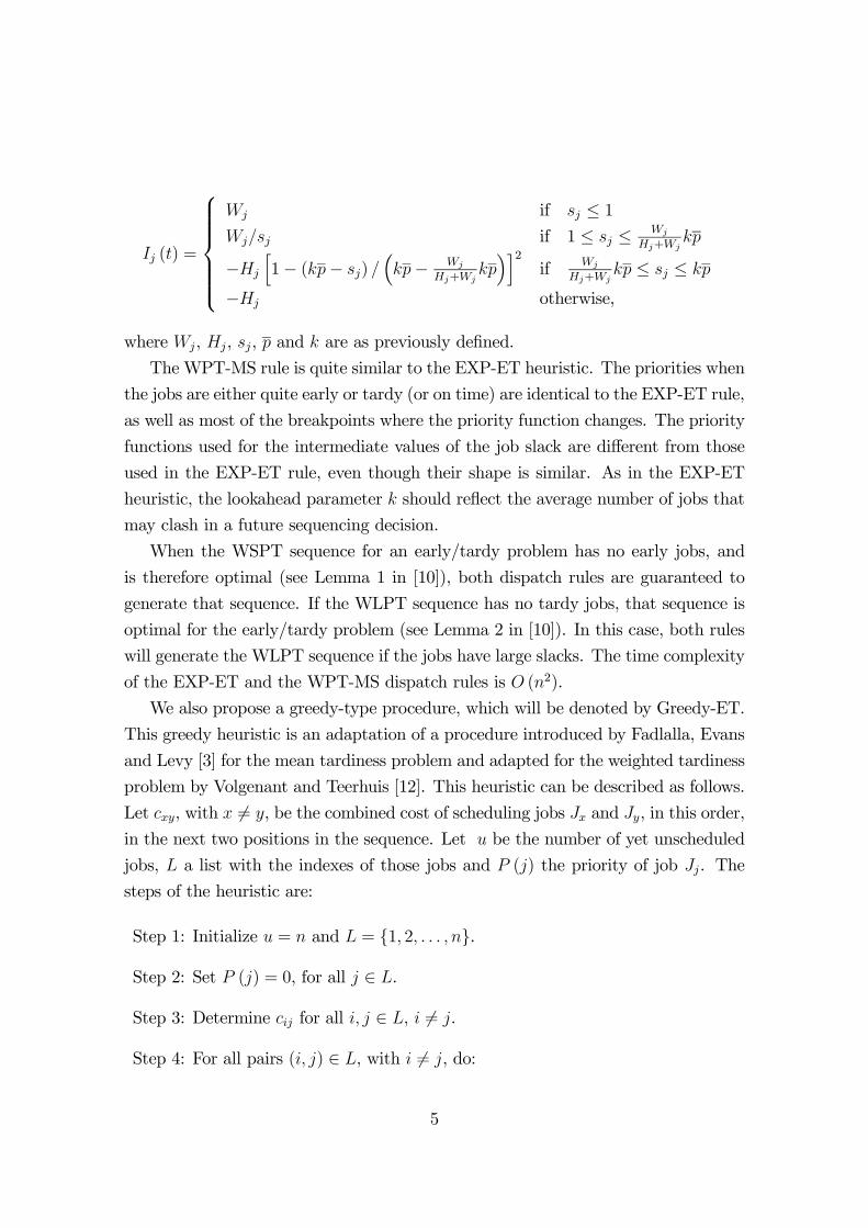
Ij (t) =

Wj if sj ≤ 0Wj exp

h− (Hj+Wj)

Hj(sj/kp)

iif 0 ≤ sj ≤ Wj

Hj+Wjkp

H−2j

hWj − (Hj+Wj)sj

kp

i3if Wj

Hj+Wjkp ≤ sj ≤ kp

−Hj otherwise,

where Wj = wj/pj, Hj = hj/pj, sj = dj − t − pj is the slack of job Jj at time t, p

is the average processing time and k is a lookahead parameter. The EXP-ET rule

reflects a priority that focuses on the tardiness cost of a job as its slack becomes

small, while the earliness cost dominates when that slack is large. The choice of the

lookahead parameter k should reflect the average number of jobs that may clash in

the future each time a sequencing decision is to be made.

We propose a new dispatch rule, which will be denoted by WPT-MS, since its

priority function incorporates both weighted processing time and minimum slack

components. The WPT-MS rule uses the following priority index Ij (t) to determine

the job Jj to be scheduled at any instant t when the machine becomes available:

4

Ij (t) =

Wj if sj ≤ 1Wj/sj if 1 ≤ sj ≤ Wj

Hj+Wjkp

−Hj

h1− (kp− sj) /

³kp− Wj

Hj+Wjkp´i2

if Wj

Hj+Wjkp ≤ sj ≤ kp

−Hj otherwise,

where Wj, Hj, sj, p and k are as previously defined.

The WPT-MS rule is quite similar to the EXP-ET heuristic. The priorities when

the jobs are either quite early or tardy (or on time) are identical to the EXP-ET rule,

as well as most of the breakpoints where the priority function changes. The priority

functions used for the intermediate values of the job slack are different from those

used in the EXP-ET rule, even though their shape is similar. As in the EXP-ET

heuristic, the lookahead parameter k should reflect the average number of jobs that

may clash in a future sequencing decision.

When the WSPT sequence for an early/tardy problem has no early jobs, and

is therefore optimal (see Lemma 1 in [10]), both dispatch rules are guaranteed to

generate that sequence. If the WLPT sequence has no tardy jobs, that sequence is

optimal for the early/tardy problem (see Lemma 2 in [10]). In this case, both rules

will generate the WLPT sequence if the jobs have large slacks. The time complexity

of the EXP-ET and the WPT-MS dispatch rules is O (n2).

We also propose a greedy-type procedure, which will be denoted by Greedy-ET.

This greedy heuristic is an adaptation of a procedure introduced by Fadlalla, Evans

and Levy [3] for the mean tardiness problem and adapted for the weighted tardiness

problem by Volgenant and Teerhuis [12]. This heuristic can be described as follows.

Let cxy, with x 6= y, be the combined cost of scheduling jobs Jx and Jy, in this order,

in the next two positions in the sequence. Let u be the number of yet unscheduled

jobs, L a list with the indexes of those jobs and P (j) the priority of job Jj. The

steps of the heuristic are:

Step 1: Initialize u = n and L = 1, 2, . . . , n.

Step 2: Set P (j) = 0, for all j ∈ L.

Step 3: Determine cij for all i, j ∈ L, i 6= j.

Step 4: For all pairs (i, j) ∈ L, with i 6= j, do:

5

If cij < cji, set P (i) = P (i) + 1;

If cij > cji, set P (j) = P (j) + 1;

If cij = cji, set P (i) = P (i) + 1 and P (j) = P (j) + 1.

Step 5: Schedule job Jl for which P (l) = max Pj; j ∈ L and set L = L \ l.

Step 6: Stop if u = 1; otherwise set u = u− 1 and go to step 2.

If cij < cji, it seems better to schedule job Ji in the next position rather than job

Jj. The priority P (j) of job Jj is therefore the number of times job Jj is the preferred

job for the next position when it is compared with all other unscheduled jobs. The

Greedy-ET heuristic selects, at each iteration, the job with the highest priority

P (j). Because of the O (n2) complexity of steps 3 and 4, the overall complexity of

the heuristic is O (n3).

3 Functions for determining the value of the looka-

head parameter

The effectiveness of the two dispatch rules presented in the previous section depends

on the lookahead parameter k which, in previous studies, has been set at a fixed

value. We propose using instance statistics to calculate an appropriate value for k.

In this section we describe the experiments performed to determine the functions

which map the instance factors into an adequate value for the lookahead parameter

k. These experiments were similar for both dispatch rules.

First, we briefly describe the factors or statistics that characterize an instance

and may affect the choice of k. The instance size n and variability of the processing

times pj and the penalties hj and wj may influence the most effective value of

k. The remaining two factors, which are associated with the due dates, are the

lateness factor LF and the range of due dates RDD. The factor LF can be defined

as LF = 1 − ¡d/Cmax¢, where d is the average of the due dates and Cmax is the

makespan. If LF is high (low), the average due date will be low (high), and most

of the jobs will likely be tardy (early). When LF assumes an intermediate value,

the number of early jobs and the number of tardy jobs in a schedule should be

relatively similar. The factor RDD, which is a measure of the due dates dispersion

6

around their average, is defined as (dmax − dmin) /Cmax, where dmax and dmin are,

respectively, the maximum and the minimum value of the due dates.

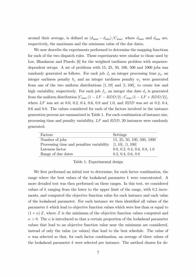
We now describe the experiments performed to determine the mapping functions

for each of the two dispatch rules. These experiments were similar to those used by

Lee, Bhaskaran and Pinedo [6] for the weighted tardiness problem with sequence-

dependent setups. A set of problems with 15, 25, 50, 100, 500 and 1000 jobs was

randomly generated as follows. For each job Jj an integer processing time pj, an

integer earliness penalty hj and an integer tardiness penalty wj were generated

from one of the two uniform distributions [1, 10] and [1, 100], to create low and

high variability, respectively. For each job Jj, an integer due date dj is generated

from the uniform distribution [Cmax (1− LF −RDD/2) , Cmax (1− LF +RDD/2)],

where LF was set at 0.0, 0.2, 0.4, 0.6, 0.8 and 1.0, and RDD was set at 0.2, 0.4,

0.6 and 0.8. The values considered for each of the factors involved in the instance

generation process are summarized in Table 1. For each combination of instance size,

processing time and penalty variability, LF and RDD, 20 instances were randomly

generated.

Factors SettingsNumber of jobs 15, 25, 50, 100, 500, 1000Processing time and penalties variability [1, 10], [1, 100]Lateness factor 0.0, 0.2, 0.4, 0.6, 0.8, 1.0Range of due dates 0.2, 0.4, 0.6, 0.8

Table 1: Experimental design

We first performed an initial test to determine, for each factor combination, the

range where the best values of the lookahead parameter k were concentrated. A

more detailed test was then performed on these ranges. In this test, we considered

values of k ranging from the lower to the upper limit of the range, with 0.2 incre-

ments, and computed the objective function value for each instance and each value

of the lookahead parameter. For each instance we then identified all values of the

parameter k which lead to objective function values which were less than or equal to

(1 + α)Z, where Z is the minimum of the objective function values computed and

α > 0. The α is introduced so that a certain proportion of the lookahead parameter

values that lead to an objective function value near the minimum are considered,

instead of only the value (or values) that lead to the best schedule. The value of

α was selected so that, for each factor combination, an average of three values of

the lookahead parameter k were selected per instance. The method chosen for de-

7

termining the value of α automatically compensates for the different variability the

objective function value may exhibit for different factor combinations. The average

of the lookahead parameter values selected for each instance is taken as the best

estimate of k for that instance. The best estimate of the parameter k for a given

factor combination is then given by the average of the best estimates for all twenty

instances sharing that factor combination.

From the results of these experiments we could conclude the following. The

processing time and penalty variability did not have a significant impact on k. The

value of k was, however, sensitive to the remaining instance factors (instance size,

LF and RDD). These factors were interrelated, since the magnitude of the effect

on k, as well as sometimes the direction of that effect, also depended on the values

of the other factors. We then decided that a single formula would fail to capture the

variety of effects and interactions among the factors, and therefore chose to develop

some functions that, although somewhat cumbersome, would more accurately reflect

the impact of the instance factors on k. All the previous comments are equally valid

for both heuristics, even though the specific functions are different.

For each heuristic we then derived a formula for each of the LF values considered

in our experiment. These formulas determine the value of k as a function of the

instance size n and RDD. Interpolation is used to determine the value of k for other

values of LF . The formulas derived for the EXP-ET and the WPT-MS heuristics

are provided in tables 2 and 3, respectively. We also remark that, for some values

of LF , not one but several functions are provided, each corresponding to a value (or

sometimes range) of the RDD factor. In these cases, the value of k for other RDD

values is once again obtained by interpolation. The experiments also showed that

the best values of k are rarely below 0.5. Therefore, if the function ever returns a

value lower than 0.5, k is set to 0.5 instead.

4 Dominance rules

In this section we present the dominance rules used to improve the schedule gen-

erated by the heuristics. Ow and Morton [10] proved that in an optimal schedule

all adjacent pairs of jobs Ji and Jj, with Ji preceding Jj, must satisfy the following

condition:

wipj − Ωij (wi + hi) ≥ wjpi − Ωji (wj + hj)

8

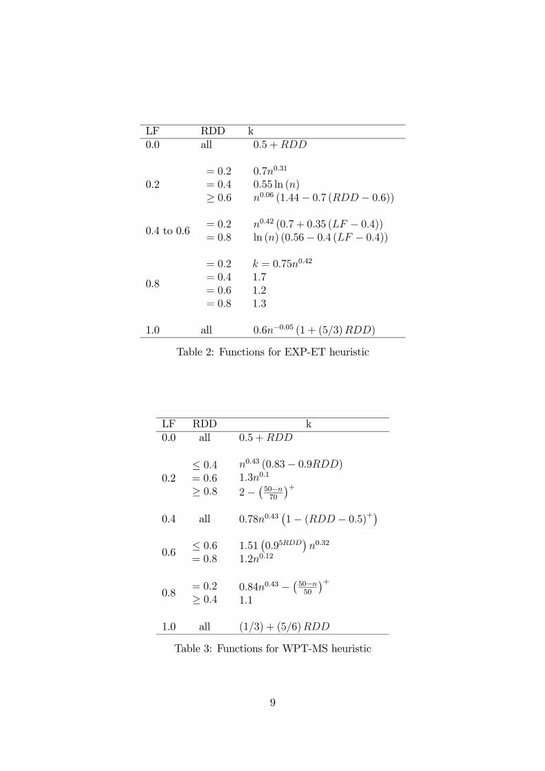
LF RDD k0.0 all 0.5 +RDD

0.2= 0.2= 0.4≥ 0.6

0.7n0.31

0.55 ln (n)n0.06 (1.44− 0.7 (RDD − 0.6))

0.4 to 0.6= 0.2= 0.8

n0.42 (0.7 + 0.35 (LF − 0.4))ln (n) (0.56− 0.4 (LF − 0.4))

0.8

= 0.2= 0.4= 0.6= 0.8

k = 0.75n0.42

1.71.21.3

1.0 all 0.6n−0.05 (1 + (5/3)RDD)

Table 2: Functions for EXP-ET heuristic

LF RDD k0.0 all 0.5 +RDD

0.2≤ 0.4= 0.6≥ 0.8

n0.43 (0.83− 0.9RDD)1.3n0.1

2− ¡50−n70

¢+0.4 all 0.78n0.43

¡1− (RDD − 0.5)+¢

0.6≤ 0.6= 0.8

1.51¡0.95RDD

¢n0.32

1.2n0.12

0.8= 0.2≥ 0.4

0.84n0.43 − ¡50−n50

¢+1.1

1.0 all (1/3) + (5/6)RDD

Table 3: Functions for WPT-MS heuristic

9

with Ωxy defined as

Ωxy =

0 if sx ≤ 0,sx if 0 < sx < py,

py otherwise,

where sx = dx− t− px is the slack of job Jx and t is the sum of the processing times

of all jobs preceding Ji.

Liaw [9] demonstrated that all non-adjacent pairs of jobs Ji and Jj, with pi = pj

and Ji preceding Jj, must satisfy the following condition in an optimal schedule:

wi (pj +∆)− Λij (wi + hi) ≥ wj (pi +∆)− Λji (wj + hj)

where ∆ is the sum of the processing times of all jobs between Ji and Jj and Λxy is

defined as

Λxy =

0 if sx ≤ 0,sx if 0 < sx < py +∆,

py +∆ otherwise,

where sx and t are defined as before.

After a heuristic has generated a schedule, these rules are applied as follows.

First, the adjacent dominance rule of Ow and Morton is used. When a pair of

adjacent jobs violates that rule, those jobs are swapped. This procedure is repeated

until no improvement is found by the adjacent rule in a complete iteration. Then

the non-adjacent rule is applied. Once again, if a pair of jobs violates the rule those

jobs are swapped, and the procedure is repeated until no improvement is made in a

complete iteration. The above two steps are repeated while the number of iterations

performed by the non-adjacent rule is greater than one (i.e., while that rule detects

an improvement).

5 Computational results

In this section we present the results from the computational tests. The set of

test problems was generated as described in section 3. All the algorithms were

coded in Visual C++ 6.0 and executed on a Pentium IV-1500 personal computer.

Throughout this section, and in order to keep the table sizes reasonable, we will

sometimes present results only for some representative cases. We first compare the

10

function-based versions of the EXP-ET and WPT-MS heuristics with their fixed-

value counterparts. Four fixed values of k were used for this purpose: 3, 5, 7 and

9. The first two had already been considered in [10]. The other two values were

included since some of our test instances have a much larger size, and k should

usually increase with the instance size. In the following, and for each combination

of instance size and penalty variability, we will present results for the fixed value

that leads to the lowest average objective function value across all such instances.

In table 4 we present the average objective function value (mean ofv) for both

versions and the average of the relative differences in objective function values (avg %

ch.), calculated as F−KK∗100, where F andK are the objective values of the function

and fixed value versions, respectively. Table 5 gives the number of instances for which

the function-based version performs better (<), equal (=) or worse (>) than the

fixed-value version. We also performed a test to determine if the difference between

the two versions is statistically significant. Given that the heuristics were used on

exactly the same problems, a paired-samples test is appropriate. Since some of the

hypothesis of the paired-samples t-test were not met, the non-parametric Wilcoxon

test was selected. Table 5 also includes the significance (sig.) values of this test,

i.e., the confidence level values above which the equal distribution hypothesis is to

be rejected. From the results presented in these two tables, we can conclude that

the function-based versions outperform their fixed value counterparts, since their

average objective function value is lower and they provide better results for most

of the test instances. The Wilcoxon test values also indicate that the difference in

distribution between the two versions is statistically significant. We also compared

the function and fixed value versions of the heuristics on instances with LF and

RDD values of 0.1, 0.3, 0.5, 0.7 and 0.9. The results were similar to those just

presented, thus confirming the superior performance of the proposed formulas.

We now compare the several heuristics and analyse the effect of the dominance

rules. In table 6 we present the average objective function value (mean ofv) for each

heuristic, both without and with the dominance rules, and the average of the relative

differences in objective function values (avg % ch.), calculated as HDR−HH∗100, where

H and HDR are the objective function values of a heuristic without and with the

dominance rules, respectively. We also give the number of times each heuristic

produces the best result when compared with the other heuristics, both before and

after the use of the dominance rules. The best results for both the objective function

value, and the number of times each heuristic is the best, are presented in bold. A

11

mean ofvvar. Heuristic n function best k avg % ch.1-10 EXP-ET 15 1263 1300 -3,84

50 12887 12970 -0,58500 1239595 1241411 -0,16

WPT-MS 15 1258 1278 -1,9250 12831 12900 -0,50500 1237086 1240158 -0,29

1-100 EXP-ET 15 98358 101202 -3,7750 1000355 1008409 -0,86500 95009775 95128094 -0,11

WPT-MS 15 99533 100853 -1,8050 1004379 1008680 -0,42500 94872887 95149062 -0,39

Table 4: Function vs fixed value: average objective function value and relativedifference

function vs best kvar. Heuristic n < = > sig.1-10 EXP-ET 15 339 74 67 0,000

50 350 16 114 0,000500 371 5 104 0,000

WPT-MS 15 213 230 37 0,00050 277 92 111 0,000500 406 4 70 0,000

1-100 EXP-ET 15 361 49 70 0,00050 364 23 93 0,000500 364 4 112 0,000

WPT-MS 15 182 249 49 0,00050 212 171 97 0,000500 350 57 73 0,000

Table 5: Function vs fixed value: objective function value comparison and statisticaltest

12

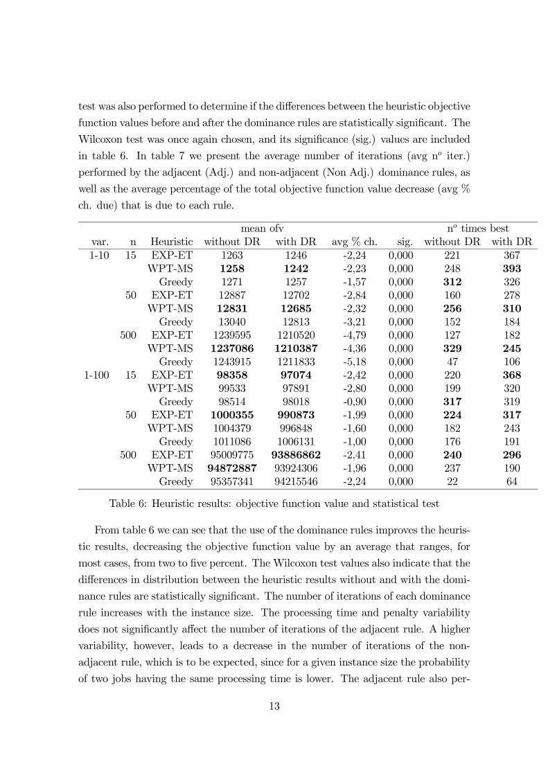
test was also performed to determine if the differences between the heuristic objective

function values before and after the dominance rules are statistically significant. The

Wilcoxon test was once again chosen, and its significance (sig.) values are included

in table 6. In table 7 we present the average number of iterations (avg no iter.)

performed by the adjacent (Adj.) and non-adjacent (Non Adj.) dominance rules, as

well as the average percentage of the total objective function value decrease (avg %

ch. due) that is due to each rule.

mean ofv no times bestvar. n Heuristic without DR with DR avg % ch. sig. without DR with DR1-10 15 EXP-ET 1263 1246 -2,24 0,000 221 367

WPT-MS 1258 1242 -2,23 0,000 248 393Greedy 1271 1257 -1,57 0,000 312 326

50 EXP-ET 12887 12702 -2,84 0,000 160 278WPT-MS 12831 12685 -2,32 0,000 256 310Greedy 13040 12813 -3,21 0,000 152 184


1-100 15 EXP-ET 98358 97074 -2,42 0,000 220 368WPT-MS 99533 97891 -2,80 0,000 199 320Greedy 98514 98018 -0,90 0,000 317 319



Table 6: Heuristic results: objective function value and statistical test

From table 6 we can see that the use of the dominance rules improves the heuris-

tic results, decreasing the objective function value by an average that ranges, for

most cases, from two to five percent. The Wilcoxon test values also indicate that the

differences in distribution between the heuristic results without and with the domi-

nance rules are statistically significant. The number of iterations of each dominance

rule increases with the instance size. The processing time and penalty variability

does not significantly affect the number of iterations of the adjacent rule. A higher

variability, however, leads to a decrease in the number of iterations of the non-

adjacent rule, which is to be expected, since for a given instance size the probability

of two jobs having the same processing time is lower. The adjacent rule also per-

13

avg no iter. avg % ch. duevar. n Heuristic Adj. Non Adj. Adj. Non Adj.1-10 15 EXP-ET 1,9 1,2 91,22 8,78

WPT-MS 1,9 1,2 93,36 6,64Greedy 1,4 1,2 76,94 23,06

50 EXP-ET 3,4 1,9 83,19 16,81WPT-MS 3,3 1,8 84,26 15,74Greedy 2,9 2,2 61,39 38,61


1-100 15 EXP-ET 1,8 1,0 99,81 0,19WPT-MS 1,8 1,0 98,40 1,60Greedy 1,3 1,0 95,71 4,29



Table 7: Dominance rules: iterations and relative importance

forms a larger number of iterations than the non adjacent rule. The percentage of

the total objective function value improvement that is due to the non-adjacent rule

increases with the instance size, which agrees with the higher probability of equal

processing times, and is higher for the Greedy heuristic. From the objective func-

tion values, and the number of times each heuristic is the best, we can also conclude

the following. The WPT-MS is the best-performing heuristic when the processing

time and penalty variability is low. The EXP-ET heuristic usually provides the best

results for a high variability, being only equalled or surpassed by the WPT-MS for

the largest instance sizes.

In tables 8 and 9 we present the effect of the LF and RDD values on the

relative objective function value difference, and the number of iterations performed

by each rule, respectively. These tables give results for the EXP-ET heuristic on

instances with 50 jobs and low processing time and penalty variability. The number

of iterations of each dominance rule and the relative difference in objective function

values clearly decrease as LF moves towards its extreme values. These results are to

be expected, since the heuristics, particularly the dispatch rules, are more likely to

be closer to the optimum for the extreme LF values, where the early/tardy problem

14

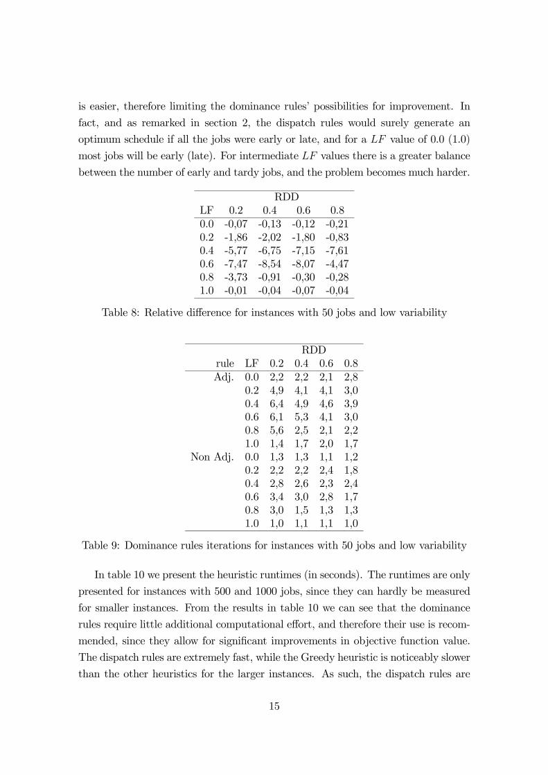
is easier, therefore limiting the dominance rules’ possibilities for improvement. In

fact, and as remarked in section 2, the dispatch rules would surely generate an

optimum schedule if all the jobs were early or late, and for a LF value of 0.0 (1.0)

most jobs will be early (late). For intermediate LF values there is a greater balance

between the number of early and tardy jobs, and the problem becomes much harder.

RDDLF 0.2 0.4 0.6 0.80.0 -0,07 -0,13 -0,12 -0,210.2 -1,86 -2,02 -1,80 -0,830.4 -5,77 -6,75 -7,15 -7,610.6 -7,47 -8,54 -8,07 -4,470.8 -3,73 -0,91 -0,30 -0,281.0 -0,01 -0,04 -0,07 -0,04

Table 8: Relative difference for instances with 50 jobs and low variability

RDDrule LF 0.2 0.4 0.6 0.8Adj. 0.0 2,2 2,2 2,1 2,8

0.2 4,9 4,1 4,1 3,00.4 6,4 4,9 4,6 3,90.6 6,1 5,3 4,1 3,00.8 5,6 2,5 2,1 2,21.0 1,4 1,7 2,0 1,7

Non Adj. 0.0 1,3 1,3 1,1 1,20.2 2,2 2,2 2,4 1,80.4 2,8 2,6 2,3 2,40.6 3,4 3,0 2,8 1,70.8 3,0 1,5 1,3 1,31.0 1,0 1,1 1,1 1,0

Table 9: Dominance rules iterations for instances with 50 jobs and low variability

In table 10 we present the heuristic runtimes (in seconds). The runtimes are only

presented for instances with 500 and 1000 jobs, since they can hardly be measured

for smaller instances. From the results in table 10 we can see that the dominance

rules require little additional computational effort, and therefore their use is recom-

mended, since they allow for significant improvements in objective function value.

The dispatch rules are extremely fast, while the Greedy heuristic is noticeably slower

than the other heuristics for the larger instances. As such, the dispatch rules are

15

clearly preferable to the greedy heuristic, since they provide better results with a

lower computational time. If the processing time and penalty variability is known

in advance, the WPT-MS (EXP-ET) is the better choice for a low (high) variability

setting; otherwise, either can be used, since the differences are not very significant.

var.1-10 1-100

Heuristic n = 500 n = 1000 n = 500 n = 1000EXP-ET 0,006 0,024 0,007 0,026

EXP-ET + DR 0,037 0,184 0,016 0,075WPT-MS 0,006 0,026 0,006 0,025

WPT-MS + DR 0,035 0,181 0,015 0,073Greedy 6,120 49,126 6,085 48,863

Greedy + DR 6,151 49,293 6,095 48,914

Table 10: Runtimes (in seconds)

We also compared the heuristic results with the optimum objective function value

for instances with 15 and 25 jobs. In tables 11 and 12 we present results for the

average of the relative deviations from the optimum, calculated as H−OO∗100, where

H and O are the heuristic and optimum objective function values, respectively.

In table 12 we present the effect of the LF and RDD values. This table only

gives results for the EXP-ET + DR heuristic and instances with 15 jobs and low

processing time and penalty variability. The best dispatch rule, when followed by

the application of the dominance rules, provides results that are less than 5% and

7% from the optimum, for low and high processing time and penalty variability,

respectively. All the heuristics are closer to the optimum when the variability is

low. As for the effect of the LF and RDD factors, it can be seen that the LF

parameter has a significant impact on the relative distance to the optimum. The

heuristic performance is at its worst for the intermediate LF values, and improves

substantially as the LF approaches its extreme values. These results are once again

expected, since the problem is harder for the intermediate LF values.

6 Conclusion

In this paper we introduced two new heuristics, a dispatch rule and a greedy-type

procedure, and also considered the best of the existing dispatch rules. For both

dispatch rules we presented functions that use the instance statistics to determine

16

var.1-10 1-100

Heuristic n = 15 n = 25 n = 15 n = 25EXP-ET 7,6 8,5 9,7 9,4WPT-MS 6,9 7,2 12,4 11,3Greedy 9,1 10,8 10,3 12,4

EXP-ET + DR 4,9 5,6 6,7 6,9WPT-MS + DR 4,2 4,7 8,7 8,8Greedy + DR 6,9 8,0 9,1 11,5

Table 11: Relative deviation from the optimum

RDDLF 0.2 0.4 0.6 0.80.0 0,04 0,73 0,15 1,020.2 3,00 3,95 7,21 4,570.4 7,46 15,59 9,95 17,410.6 13,18 10,54 8,30 6,920.8 3,14 2,51 0,48 1,461.0 0,03 0,23 0,19 0,21

Table 12: Relative deviation from the opimum for instances with 15 jobs and lowvariability

the value of a lookahead parameter that had previously been set at a fixed value. We

also considered the use of dominance rules to improve the solutions obtained by all

three heuristics. The computational results show that the function-based versions

of the dispatch rules are superior to their fixed value counterparts. The use of

the dominance rules is recommended, since they improve the solution quality of all

heuristics, and the additional computation time is quite modest. The dispatch rules

provide better solutions than the greedy-type heuristic, and require less computation

time. If the variability of the processing times and penalties is known beforehand,

the new rule should be used in low variability settings, while the previously existing

heuristic is preferable under high variability conditions.

References

[1] Abdul-Razaq, T., and Potts, C. N. Dynamic programming state-space

relaxation for single machine scheduling. Journal of the Operational Research

Society 39 (1988), 141—152.

17

[2] Baker, K. R., and Scudder, G. D. Sequencing with earliness and tardiness

penalties: A review. Operations Research 38 (1990), 22—36.

[3] Fadlalla, A., Evans, J. R., and Levy, M. S. A greedy heuristic for the

mean tardiness sequencing problem. Computers and Operations Research 21

(1994), 329—336.

[4] Korman, K. A pressing matter. Video (February 1994), 46—50.

[5] Landis, K. Group technology and cellular manufacturing in the westvaco

los angeles vh department. Project report in iom 581, School of Business,

University of Southern California, 1993.

[6] Lee, Y. H., Bhaskaran, K., and Pinedo, M. A heuristic to minimize the

total weighted tardiness with sequence-dependent setups. IIE Transactions 29

(1997), 45—52.

[7] Lenstra, J. K., Rinnooy Kan, A. H. G., and Brucker, P. Complexity

of machine scheduling problems. Annals of Discrete Mathematics 1 (1977),

343—362.

[8] Li, G. Single machine earliness and tardiness scheduling. European Journal of

Operational Research 96 (1997), 546—558.

[9] Liaw, C.-F. A branch-and-bound algorithm for the single machine earliness

and tardiness scheduling problem. Computers and Operations Research 26

(1999), 679—693.

[10] Ow, P. S., and Morton, E. T. The single machine early/tardy problem.

Management Science 35 (1989), 177—191.

[11] Valente, J. M. S., and Alves, R. A. F. S. Improved lower bounds for

the early/tardy scheduling problem with no idle time. Working paper 125,

Faculdade de Economia do Porto, Portugal, 2003.

[12] Volgenant, A., and Teerhuis, E. Improved heuristics for the n-job single-

machine weighted tardiness problem. Computers and Operations Research 26

(1999), 35—44.

18

working papers da fep · working papers da fep ... we also con- sider the use of ... completing a...

Documents