Federal Reserve Bank of Dallas Globalization and Monetary Policy Institute

Working Paper No. 285 http://www.dallasfed.org/assets/documents/institute/wpapers/2016/0285.pdf

System Reduction and Finite-Order VAR Solution Methods for

Linear Rational Expectations Models*

Enrique Martínez-García Federal Reserve Bank of Dallas

September 2016

Abstract This paper considers the solution of a large class of linear rational expectations (LRE) models and its characterization via finite-order VARs. The solution of the canonical LRE model can be cast in state-space form and solved for by the method of undetermined coefficients. In this paper I propose an approach that simplifies the systematic characterization of the solution into finite-order VAR form and checks existence and uniqueness based on the solution of a companion Sylvester equation. Solving LRE models with a finite-order VAR representation via the Sylvester equation is straightforward to implement, efficient, and can be handled easily with standard matrix algebra. An application to the workhorse New Keynesian model with accompanying Matlab codes is provided to illustrate the implementation of the procedure in practice. JEL codes: C32, C62, C63, E37

* Enrique Martínez-García, Federal Reserve Bank of Dallas, Research Department, 2200 N. Pearl Street, Dallas, TX 75201. 214-922-5762. enrique.martinez-garcia@dal.frb.org. I would like to thank Nathan Balke, Jesús Fernández-Villaverde, Andrés Giraldo, Ayse Kabukcuoglu, María Teresa Martínez-García, Mike Plante, Michael Sposi, Mark Wynne, Carlos Zarazaga and seminar and conference participants for helpful suggestions and comments. All codes for this paper are publicly available in the following website: https://sites.google.com/site/emg07uw/. The codes can be downloaded using the following link: https://sites.google.com/site/emg07uw/econfiles/LRE_model_solution.zip?attredirects=0. I acknowledge the excellent research assistance provided by Valerie Grossman, and the help of Arthur Hinojosa. All remaining errors are mine alone. The views expressed in this paper are those of the author and do not necessarily reflect the views of the Federal Reserve Bank of Dallas or the Federal Reserve System.

1 Introduction

Many rational expectations macro models can be cast as a linear system of expectational di¤erence equations.

The linearity of the system may be a feature of the model itself but, often, is attained by means of an

approximation. In either case, the solution of linear or linearized rational expectations (LRE) models is

an important part of modern macroeconomics. Blanchard and Kahn (1980) established the conditions for

existence and uniqueness of a solution to the canonical LRE model (see also, among others, the related

methodological contributions of King and Watson (1998), Uhlig (1999), and Klein (2000)). More recently,

Fernández-Villaverde et al. (2007), Ravenna (2007), and Franchi and Paruolo (2015) have explored the

conditions under which the canonical LRE model solution permits a VAR representation which facilitates

the recovery of fundamental shocks.

The structural shocks of the LRE model cannot always be recovered from a VAR speci�cation due to lack

of fundamentalness, though. A model is said to be fundamental if there exists a (possibly in�nite-order) VAR

representation for the observables with respect to the structural shocks (Hansen and Sargent (1980)). When

the number of shocks is equal to the number of observables, the fundamentalness property of the solution

can be checked with the �poor man�s invertibility condition�of Fernández-Villaverde et al. (2007). Ravenna

(2007) proposes a �unimodularity condition�to check when the VAR representation of the LRE solution is of

�nite order. Franchi and Paruolo (2015), then, come to show that if the linear state-space form of the LRE

solution is minimal, the �poor man�s invertibility condition�and the �unimodularity condition�are necessary

and su¢ cient to ensure both fundamentalness and the existence of a �nite-order VAR representation for the

solution to the LRE model.

In this paper, I complement this literature with a novel approach to characterize� for a large class of

LRE models� the unique solution in �nite-order VAR form via a companion quadratic matrix equation and a

companion Sylvester equation. I also propose a set of straightforward conditions to check the properties� of

existence and uniqueness� of a �nite-order VAR solution. LRE models that include backward-looking and

forward-looking features with one or more lags and leads can be reduced to the canonical form given by

an expectational �rst-order di¤erence equation without backward-looking terms. After system reduction is

achieved after solving the companion quadratic matrix equation, the method of undetermined coe¢ cients

can be used to solve the canonical forward-looking part of the LRE model. Conditions under which a �nite-

order VAR representation of the LRE model solution can be obtained and a simple (yet e¢ cient) algorithm

to compute it can then be derived from a companion Sylvester equation.

The system reduction involves the solution of a quadratic matrix equation, and permits generalizing the

approach (and the algorithms) I propose in this paper to cover a wider range of LRE models (Binder and

Pesaran (1995, 1997)). One of the important contribution of the paper, though, is that the characterization

of the �nite-order VAR solution of the forward-looking part of the model arises from an associated matrix

equation� the well-known Sylvester matrix equation. I propose a simple approach based on this companion

Sylvester equation to check for and identify LRE solutions in �nite-order VAR form as well as a related

algorithm to compute such solutions.

The solution method proposed in this paper based on the companion Sylvester equation� augmented

with a companion quadratic matrix equation to handle backward-looking components� equips economists

with a straightforward way to e¢ ciently solve a large class of multivariate LRE models with multiple leads

and lags. In this paper, I illustrate this approach based on the companion Sylvester equation with the

1

workhorse three-equation New Keynesian model� showing how the procedure is used to derive the �nite-

order VAR representation of the LRE solution, to establish its existence and uniqueness, and to make

economically-relevant inferences about the New Keynesian transmission mechanism for (and the identi�cation

of) structural shocks.

The rest of the paper proceeds as follows: Section 2 describes the system reduction method to decouple the

backward-looking and forward-looking parts and shows how to use the method of undetermined coe¢ cients

to characterize the linear state-space form solution of the forward-looking part of the canonical LRE model.

Section 3 describes the mapping of the LRE model solution into a �nite-order VAR via a companion Sylvester

equation. This section also discusses the conditions under which a �nite-order VAR solution can be attained

from the companion Sylvester equation as well as the algorithms available to compute it. Section 4 applies the

method to an economically-interesting example on the e¤ects of monetary policy on in�ation determination

based on the workhorse three-equation New Keynesian model with which I also illustrate the computational

e¢ cacy of the approach. Section 5 then concludes.

The Appendix provides additional technical details on the system reduction approach used in this paper

to isolate the forward-looking part of the LRE model� including a generalized eigenvalue problem algorithm

to implement it� and also discusses related technical features of the linear state-space form of the solution

and the general form of the LRE models for which the procedure can be utilized.

2 The Canonical LRE Model

Going from the structural relationships implied by the LRE model to a reduced-form solution requires

explicit assumptions about the formation of expectations and the stochastic process of the exogenous driving

variables. The structural relationships implied by the LRE model are always true according to theory, but the

reduced-form solution of the model may depend on those assumptions. Here, I consider LRE models where

expectations are fully rational and the exogenous driving variables are assumed to follow a VAR process.

Often, a link arises between the reduced-form solution and a VAR representation for the endogenous variables

under those assumptions that can explain why VARs appear to �t the data well, while providing researchers

with a better tool for policy analysis than that of an unrestricted VAR.

Under rational expectations, agents understand the structure of the economy and formulate expectations

optimally incorporating all available information.1 Hence, the LRE model solution generally varies across

alternative policy regimes and also as a result of variations in expectations about the future induced by

policy changes. Ultimately, the assessment of an LRE model must be based upon its ability to capture

the relevant aspects of the macro data. However, reduced-form econometric models �tted to historical data

(unrestricted VARs) may describe the data well and still be of limited use for policy analysis without the

structure imposed by theory� as stressed by Lucas (1976). In this paper, I explore the connection between

the reduced-form solution of LRE models and VARs to help bridge the gap between theoretical and applied

work towards a more uni�ed approach (for testing the cross-equation restrictions imposed by theory and for

policy analysis).

A large class of LRE models can be cast into a canonical system of expectational di¤erence equations,

1The idea of rational expectations can be traced to the seminal work by Muth (1961). Lucas (1976) and Sargent (1980) wereamong the leading economists that rejected ad hoc assumptions on the formation of expectations and advocated the adoptionof rational expectations that became prevalent in modern macroeconomics since the 80s.

2

featuring forward- and backward-looking dynamics. The expectational di¤erence equations capture the

structural relationships between a set of k endogenous variables Wt = (w1t; w2t; :::; wkt)T and k exogenous

driving variables Xt = (x1t; x2t; :::; xkt)T as follows:

Wt = �1Wt�1 +�2Et [Wt+1] + �3Xt; (1)

where �1, �2, and �3 are conforming k � k square matrices.2 The remaining p endogenous variables of theLRE model fWt = ( ew1t; ew2t; :::; ewpt)T can then be expressed as functions of Wt and Xt, possibly including

lags and expectations of their leads too.

I complete the speci�cation of the canonical form of the LRE model given by (1) with a standard VAR(1)

speci�cation for the vector of k driving variables Xt of the following form:

Xt = AXt�1 +B�t; (2)

where A is a k�k matrix that has all its eigenvalues inside the unit circle, B is a k�k matrix that describesthe matrix of variances and covariances, and �t is the corresponding vector of innovations of dimension k.

The conventional method to characterize a reduced-form solution for a forward-looking LRE model is laid

out in Blanchard and Kahn (1980), which also provide conditions to check the existence and uniqueness of the

solution. Blanchard and Kahn�s (1980) method was further re�ned by Broze et al. (1985, 1990), King and

Watson (1998), Uhlig (1999), and Klein (2000) among others, to obtain solutions in more general settings.

Other popular solution methods applied to LRE models include the method of undetermined coe¢ cients

of Christiano (2002) and the method of rational expectational errors of Sims (2002) (see also Lubik and

Schorfheide (2003)).

2.1 Decoupling Backward- and Forward-Looking Terms

The quadratic determinantal equation (QDE) method of Binder and Pesaran (1995, 1997) builds on Broze

et al. (1985, 1990), but deals explicitly with the simultaneous dependence of Wt on its past and on its future

expected values given by the canonical form in (1). I adopt a key aspect of the QDE method implementing

a simple transformation of (1) that achieves a system reduction excluding all backward-looking terms from

the expectational di¤erence system and then I work out the LRE model solution by parts.

For a given k � k matrix �, the proposed transformation of the endogenous variables given by Wt =

Zt +�Wt�1 implies that the expectational di¤erence system in (1) can be rewritten as

Zt +�Wt�1 = �1Wt�1 +�2Et [Zt+1 +�Wt] + �3Xt

= �1Wt�1 +�2 [Et (Zt+1) + � (Zt +�Wt�1)] + �3Xt; (3)

which then becomes

(Ik � �2�)Zt = �2Et (Zt+1) +��2�

2 ��+�1�Wt�1 +�3Xt: (4)

2Here, I consider the case where the number of endogenous and exogenous variables in (1)� (2) is the same� hence, if thesolution can be represented in VAR form, it can be exploited to recover the fundamental economic shocks included in the model.Notice that the canonical form in (1)� (2) can be generalized to capture LRE models including more than one lead and lag inthe speci�cation, as explained in the Appendix.

3

From here, this condition follows:

Condition 1 A system reduction that excludes the backward-looking terms in (1) can be attained by choosinga k � k matrix � to satisfy that

P (�) = �2�2 ��+�1 = 0k; (5)

where 0k is a square k � k matrix of zeroes.

This transformation uncouples the solution of (1) into a backward-looking part, Wtb = �Wt�1, and a

forward-looking part, Wtf = Zt, such thatWt =Wtb+Wtf . Hence, to solve the canonical LRE model in (1),

one �rst needs to determine the matrix � solving the quadratic matrix equation in (5) to characterize the

backward-looking part of the solution and reduce the canonical system to its purely forward-looking expec-

tational di¤erence part. Binder and Pesaran (1995, 1997) establish the necessary and su¢ cient conditions

under which real-valued solutions for � satisfying (5) exist and provide a straightforward iterative algorithm

to compute its stable solution. A discussion of an alternative algorithm to characterize the solution � based

on the generalized eigenvalue problem can be found in the Appendix.

After decoupling, the vector of k transformed variables Zt =Wt ��Wt�1 follows a canonical �rst-order

forward-looking expectational di¤erence system of the following form:

�0Zt = �1Et [Zt+1] + �2Xt; (6)

where �0 � (Ik � �2�), �1 � �2, and �2 � �3 are conforming k� k matrices. Whenever �0 is nonsingular,the system of structural relationships implied by (6) can be rewritten as

Zt = FEt [Zt+1] +GXt; (7)

where F � (�0)�1 �1 and G � (�0)�1 �2.The invertibility of �0 required to go from (6) to (7) depends on the choice of matrix �. Binder and

Pesaran (Proposition 2, 1997) discuss conditions under which the solution can be characterized analytically

and then provide su¢ cient conditions under which (Ik � �2�) would be nonsingular. Whenever the Binderand Pesaran (1997) conditions are satis�ed, the matrix �0 can be shown to be nonsingular and invertible.

Those conditions are only su¢ cient (not necessary), but I �nd that most well-speci�ed economic models

indeed produce a matrix �0 that is nonsingular. Hence, I take the speci�cation in (7) to constitute the

relevant benchmark to describe the forward-looking part of the LRE model solution in the remainder of this

paper.

2.2 The Method of Undetermined Coe¢ cients for Solving the LRE Model

Assuming that the Blanchard and Kahn (1980) conditions for existence and uniqueness are satis�ed, the

solution to the forward-looking part of the LRE model can be written in linear state-space form as follows:

Xt = AXt�1 +B�t; (8)

Zt = CXt�1 +D�t; (9)

4

where A, B, C, and D are conforming k�k matrices. Equation (8) simply re-states the assumption made in(2) about the dynamics of the exogenous driving variables, while (9) indicates that current innovations and

lagged exogenous driving variables are mapped into the current endogenous variables in the reduced-form

solution of the LRE model.

In order to pin down this reduced-form solution, I need to relate the unknown reduced-form coe¢ cients

C and D to the composite matrices that describe the structural relationships of the LRE model (F , G) and

those that describe the shock process of the driving variables (A, B). Using the method of undetermined

coe¢ cients, such a solution can be fully characterized via the solution of a Sylvester equation and, under

additional constraints, it can be shown to have a �nite-order VAR representation.

Step 1. Using (9) shifted one period ahead to replace Zt+1 in the purely forward-looking system of

equations given in (7) implies that:

Zt = [FC +G]Xt (10)

= [FC +G]AXt�1 + [FC +G]B�t; (11)

where the second equality from from replacing Xt out using (8). The general form of the forward-looking

LRE model solution given in (9) can be matched with (11) to link the unknown reduced-form coe¢ cients

C and D to the composite matrices that describe the LRE model (F , G, A, B). Hence, by the method of

undetermined coe¢ cients, it follows that the conforming square matrices C and D that characterize (9) in

the solution must satisfy the following conditions:

C = [FC +G]A; (12)

D = CA�1B: (13)

The eigenvalues of matrix A must be inside the unit circle by construction for the VAR(1) process of the

driving variables to be stationary. I also assume that zero is not an eigenvalue of matrix A as that ensures

the inverse matrix A�1 in (13) exists and is well-de�ned according to the Invertible Matrix Theorem.

As a result, the existence and uniqueness of a solution to C that satis�es (12) also pins down D through

(13) ensuring the existence and uniqueness of the full solution to the forward-looking part of the LRE model

given by the state-space form in (8)� (9). Hence, assuming �0 is invertible as indicated before, solving thecompanion Sylvester equation given by (12) to obtain C turns out to be enough to characterize the solution

to the forward-looking part of the LRE model in (8)� (9).Step 2. Using (8) and the invertibility of A, I can write Xt�1 as Xt�1 = A�1 (Xt �B�t). Replacing

this expression in (9), I infer that:

Zt = CA�1Xt +�D � CA�1B

��t: (14)

Then, it follows from the condition (13) that characterizes the matrix D using the method of undetermined

coe¢ cients that the term related to the vector of innovations �t must drop out from (14). As a result, the

solution of the forward-looking part of the LRE model implies a straightforward linear mapping from the

5

vector of exogenous driving variables Xt to the vector of endogenous variables Zt where

Zt = CA�1Xt; (15)

if a matrix C exists that solves the Sylvester equation implied by condition (13).

Whenever a unique C exists which can also be shown to be invertible, equation (15) implies that Xt =

AC�1Zt given that A is invertible by construction. Shifting this expression one period back and replacing

it in (9), I obtain the following VAR(1) speci�cation that characterizes the solution of the forward-looking

part of the LRE model:

Zt = CAC�1Zt�1 + CA�1B�t; (16)

where I replaced D using condition (13). The existence and uniqueness of the matrix D follows naturally

under condition (13) from the existence and uniqueness of a matrix C that solves the Sylvester equation given

by condition (12). However, I also �nd that the solution of the forward-looking part of the LRE model has

a �nite-order VAR representation given by (16) whenever a unique matrix C solving the Sylvester equation

exists which can also be shown to be invertible. Therefore, the characterization of the �nite-order VAR

solution in (16) depends on the invertibility of �0 as indicated before, but also on the existence, uniqueness,

and invertibility of the solution C arising from condition (12).

Rewriting condition (12), the characterization, existence, and uniqueness of a �nite-order VAR solution

can be summarized as follows:

Lemma 1 If �0 is invertible, a VAR(1) representation of the solution to the �rst-order expectational di¤er-ence system of equations in (7) can be obtained by solving a companion Sylvester equation in C

FCA� C = H; (17)

where

F � (�0)�1 �1; H � �GA = � (�0)�1 �2A: (18)

If a unique matrix C exists and is invertible, the VAR(1) representation of the solution is given by (16).

The proof of this lemma follows directly from the derivation of conditions (12)� (13) by the method ofundetermined coe¢ cients, as discussed above.

Step 3. Then, the solution of the full LRE model can be obtained by combining its backward- andforward-looking parts� i.e., Wt =Wtb +Wtf where the backward-looking part, Wtb = �Wt�1, follows from

the solution to the quadratic matrix equation in (5) and the forward-looking part, Wtf = Zt =Wt��Wt�1,

is de�ned by the state-space solution in (8)� (9) given conditions (12)� (13) whenever a solution C to the

companion Sylvester equation exists. Under the additional condition that C be invertible (stated in Lemma

1), the implication is that the solution of the full model must follow a VAR(2) process of the following form

Corollary 1 If a unique matrix C exists that solves the companion Sylvester equation of Lemma 1 and this

matrix is also invertible, the VAR(2) representation of the canonical LRE model solution for the vector of

endogenous variables Wt is given by

Wt = 1Wt�1 +2Wt�2 +3�t; (19)

6

where the corresponding coe¢ cient matrices are 1 ���+ CAC�1

�, 2 � �CAC�1�, and 3 � CA�1B.

The derivation of this corollary follows naturally from the de�nition of the forward-looking part of the

solution Zt as Zt = Wt � �Wt�1 and the derivation of a VAR(1) representation for Zt implied under the

terms of Lemma 1. Notice that the matrix 3 is not necessarily going to be positive-semide�nite and

symmetric, so it does not have the standard interpretation of a variance-covariance matrix unlike the matrix

B.3 However, what follows from the de�nition of 3 in Corollary 1 is that 3 is a linear transformation of

the variance-covariance matrix of the shock process B where the mapping is determined by CA�1 (which

depends on the solution C of the companion Sylvester equation).

3 The Solution to the Companion Sylvester Equation

If a solution C exists for the companion Sylvester equation given by (17), then the solution of the forward-

looking part of the LRE model given in state-space form by (8) � (9) exists. According to Lemma 1, sucha solution can be represented with a �nite-order VAR whenever C is also shown to be invertible. Hence,

the main methodological contribution of the paper is to solve a large class of LRE models that �t into the

canonical form given by (1) � (2) via a companion Sylvester equation. The corollary of the approach Ipropose is that under some additional conditions on the form of the solution to the companion Sylvester

equation, the LRE model solution admits a �nite-order VAR representation. Hence, in this section I aim

to provide some additional discussion on characterizing the solution to the Sylvester equation in (17) and

provide an overview of the e¢ cient algorithms to compute it numerically.

3.1 Characterization of the Sylvester Equation Solution

Equation (17) proposes a companion Sylvester equation� i.e., FCA � C = H with F;A;H 2 Rk�k givenand C 2 Rk�k to be determined� as an alternative to characterize the solution of the forward-looking partof the LRE model. The Sylvester equation is one of the better known matrix equations in stability and

control theory and its applications.4 Using the Kronecker (tensor) product notation and the properties of

the vectorization operator vec, I can re-write Sylvester�s equation in its standard form as a linear system of

equations:

Avec (C) = vec (H) ; (20)

A :=��AT F

�� Ik2

�; (21)

3To test whether 3 has the properties of a variance-covariance matrix, I can use the chol function in Matlab. If chol returnsa second argument that is zero from [R; p] = chol (3), then the matrix is con�rmed to be symmetric and� in this case� alsopositive de�nite.

4The Sylvester matrix equation is extensively discussed in Lancaster and Tismenetsky (1985, Chapter 12). Additional usefulreferences on the characterization of the solution to the Sylvester equation include Horn and Johnson (1991) and Jiang andWei (2003).

7

where denotes the Kronecker product.5 In this way, the Sylvester equation is represented by a linear

system of dimension k2 � k2 conformed by k2 equations in k2 unknown variables (where the unknowns

correspond to the elements of the matrix C).

Having transformed the Sylvester equation into the linear system given by (20)�(21), well-known matrixalgebra results su¢ ce to determine the following criteria for the existence and uniqueness of a solution C to

the companion Sylvester equation:

Proposition 1 Let F;A;H 2 Rk�k. Then, it follows that:(a) (Existence) The Sylvester equation in (17) has at least one solution C 2 Rk�k if and only if

rank [A vec (H)] = rank [A].(b) (Uniqueness) The Sylvester equation in (17) has a unique solution C 2 Rk�k if and only if rank [A] =

k2; that is, the solution is unique if and only if A has full rank. Then, A is nonsingular and invertible implyingthat the unique solution to the Sylvester equation can be recovered as vec (C) = A�1vec (H).

Proof. (a) Trivially it follows that rank [A vec (H)] � rank [A]. If there is a solution vec (C) =

[c1 c2 ::: ck2 ]T for the linear system given by (20)�(21), then

Xk2

i=1A�ici = vec (H) where A�1;A�2; :::;A�k2

denote the corresponding columns of the matrix A. Hence, vec (H) is a linear combination of the columnsof A and, as a result, the rank of the augmented matrix [A vec (H)] cannot be di¤erent than the rank of

A� because for rank [A vec (H)] > rank [A] to be true, vec (H) needs to be linearly independent from the

columns of A and that contradicts vec (C) being a solution.

(b) If the square matrix A has full rank� and, therefore, is nonsigular and invertible� the linear system in(20)�(21) has a unique solution given by vec (C) = A�1vec (H). The converse statement follows naturally aswell. If the linear system has a unique solution, then A must have full rank and be nonsingular. Otherwise,at least one column in A is not linearly independent from the rest of the columns and can be written as

a linear combination of them. Hence, for any given solution vec (C) de�ned over the linearly independent

columns, another di¤erent solution exists including non-trivially the linearly dependent columns of A as well.The existence of more than one solution then contradicts the uniqueness assumption.

Proposition 1 characterizes the solution C to the Sylvester equation in (17) and, by extension, determines

conditions for the existence and uniqueness of the solution to the forward-looking part of the LRE model. The

two rank conditions stated in this proposition depend solely on the properties of the matrices F;A;H 2 Rk�k

5For a given matrix X 2 Rk�k, express X = [X�1 X�2 ::: X�k] where X�j 2 Rk, j = 1; 2; :::; k. Then, the vectorizationassociated to matrix X de�nes the following vector-valued function2664

X�1X�2:::X�k

3775 2 Rk2which is denoted vec (X). The vectorization operation is linear, i.e. vec (�X + �Y ) = �vec (X)+�vec (Y ) for any X;Y 2 Rk�kand �; � 2 Rk. If X = [xij ]

ki;j=1 2 R

k�k and Y 2 Rk�k, then the Kronecker (tensor) product of X and Y , written X Y , isde�ned to be the partitioned matrix

X Y = [xijY ] =

26664x11Y x12Y ::: x1kYx21Y x22Y ::: x2kY...

......

xk1Y xk2Y xkkY

37775 2 Rk2�k2 :Proposition 4 in Chapter 12.2 of Lancaster and Tismenetsky (1985) shows that the vectorization operation is closely related tothe Kronecker product as follows: If X;Y; Z 2 Rk�k, then vec (XY Z) =

�ZT X

�vec (Y ).

8

that describe the structural relationships of the LRE model. The uniqueness rank condition implies a solution

of the form vec (C) = A�1vec (H) for the Sylvester equation and, naturally, that proves existence as well.If the uniqueness rank condition is violated, the existence rank condition determines whether there is no

solution to the companion Sylvester equation� if rank [A vec (H)] 6= rank [A]� or whether multiple solutionsexist� if rank [A vec (H)] = rank [A] < k2. In the latter case, it can be shown that the number of linearly

independent solutions is determined by the dimension of the kernel of A.The characterization of the linearly independent solutions of the companion Sylvester equation whenever

a solution exists but is not unique can be found elsewhere in Theorem 12.5.1, Theorem 12.5.2 and Corollary

12.5.1 of Lancaster and Tismenetsky (1985). Focusing on the case of interest for this paper where a solution

for the Sylvester equation in (17) exists and is unique, the full rank condition on A can be expressed in

terms of the eigenvalues of F and A as follows:

Proposition 2 Let F;A 2 Rk�k be given. Let �1; :::; �k be the eigenvalues of F and �1; :::; �k the eigenvaluesof A. Then, for any matrix H 2 Rk�k, it follows that the companion Sylvester equation in (17) has a uniquesolution if and only if �i�j 6= 1 for all i; j = 1; :::; k. In other words, the Sylvester equation has a unique

solution C 2 Rk�k if and only if the matrices F and A�1 have no eigenvalues in common.

Proof. The eigenvalues of A are the same as those of its transpose AT . Given that and the properties

of the Kronecker product, the eigenvalues of�AT F

�are the k2 numbers de�ned by the product between

the eigenvalues of F and A, i.e., �i�j for all i; j = 1; :::; k . Then, the eigenvalues of A :=��AT F

�� Ik2

�are simply the k2 numbers �i�j � 1 for all i; j = 1; :::; k. By Proposition 1, the existence and uniqueness

of a solution to the Sylvester equation requires A to be nonsingular (and have full rank). The matrix A is

nonsingular if and only if all its eigenvalues are nonzero, i.e. if and only if �i�j � 1 6= 0 for all i; j = 1; :::; k.Re-arranging the nonzero conditions on the eigenvalues, it follows that �i 6= 1

�jfor all i; j = 1; :::; k. Given

that the eigenvalues of A�1 are 1�1; :::; 1

�kwhile those of F are �1; :::; �k, a unique solution is said to exist if

and only if indeed the matrices F and A�1 have no eigenvalues in common.

According to Proposition 2, the companion Sylvester equation for the forward-looking part of the LRE

model has a unique solution C for each matrix H if and only if F and A�1 have no eigenvalues in common.

The Sylvester operator S : Rk�k ! Rk�k can be de�ned as follows:

S (C) = FCA� C; (22)

where F;A 2 Rk�k are given and C 2 Rk�k is the solution to be identi�ed. Then, the Sylvester equationcan simply be written as S (C) = H for any given H 2 Rk�k.The k2 eigenvalues of the Sylvester operator S (C) are �i�j � 1, for all i; j = 1; :::; k, where �1; :::; �k are

the eigenvalues of F , and �1; :::; �k are the eigenvalues of A. Let vi be the right eigenvector of F associated

with the eigenvalue �i such that Fvi = �ivi for all i = 1; :::; k. Let wj be the left eigenvector of A associated

with the eigenvalue �j such that wTj A = �jwTj for all j = 1; :::; k. Then, for any i; j = 1; :::; k, C = viw

Tj

is an eigenvector matrix of the Sylvester operator S (C) associated with its eigenvalue �i�j � 1. It follows

9

from here that the Sylvester operator can be expressed as:

S (C) = FCA� C = F�viw

Tj

�A� viwTj

= (Fvi)�wTj A

�� viwTj

= (�ivi)��jw

Tj

�� viwTj

= (�i�j � 1) viwTj= (�i�j � 1)C: (23)

Hence, it can be shown that the Sylvester operator S (C) must be nonsingular whenever �i�j 6= 1 for all

i; j = 1; :::; k; that is, S (C) is nonsingular if and only if the solution to the Sylvester equation exists and is

unique.

The eigenvalues of A, �1; :::; �k, are all inside the unit circle by construction to ensure the stochastic

process for the driving variables is stationary and none of those eigenvalues is 0 so A is invertible. However,

the conditions for existence and uniqueness of the Sylvester equation solution stated in Proposition 2 do not

require the eigenvalues of F , �1; :::; �k, to be inside the unit circle. Imposing additional restrictions on the

eigenvalues of F , an explicit form for the solution C of the Sylvester equation in (17) can be obtained as

follows:

Proposition 3 Let F;A 2 Rk�k where �1; :::; �k are the eigenvalues of F and �1; :::; �k are the eigenvalues

of A. Then, for any matrix H 2 Rk�k, it follows that the companion Sylvester equation in (17) has a uniquesolution whenever �i�j < 1 for all i; j = 1; :::; k and this solution is given by

C = �X1

s=0F sHAs: (24)

Proof. Let me de�ne the following recursion: FCr�1A � Cr = H for iterations r = 1; 2; 3; ::: with the

initial condition C0 = 0k and 0k is a k�k matrix of zeros. If this recursion converges as r goes to in�nity, thenby construction the limit characterizes the solution of the Sylvester equation lim

r!1Cr = �

X1

s=0F sHAs = C.

The convergence condition is equivalent to lims!1

F sHAs = 0. It naturally follows that any eigenvalue of

F sHAs must be proportional to the s�power of the product between the eigenvalues of F and A, i.e.,

(�i�i)s for any i = 1; :::; k. Hence, if all cross products between the eigenvalues of F and A are strictly less

than one, the corresponding eigenvalues for F sHAs must go to zero in the limit as s!1 and this su¢ ces

to show that the recursion must converge as stated (Lancaster and Tismenetsky (1985, Chapter 12.3)).

Proposition 3 implies that whenever the product of the spectral radii of matrices A and F is strictly

less than one, a unique solution exists that takes the special form of an in�nite sum. Furthermore, this

special case permits the straightforward computation of the solution to the companion Sylvester equation

via a recursion on a convergent sequence as suggested by the proof of the proposition. I explore later on a

related numerical algorithm and other alternative e¢ cient algorithms to compute the unique solution of the

Sylvester equation in (17). Often a numerical solution rather than one in explicit form is all that is needed

to recover the forward-looking part of the LRE model.

However, even when a solution C to the companion Sylvester equation in (17) exists and is unique,

characterizing the solution of the forward-looking part of the LRE model with a �nite-order VAR form

requires C also to be nonsingular. If C can be shown to be nonsingular, its inverse C�1 can be computed in

10

order to obtain the �nite-order VAR representation of the LRE model given by Lemma 1 and Corollary 1.

Proving the existence of C and its uniqueness does not su¢ ce to ensure the solution is also invertible.

For some matrices H 2 Rk�k, the unique solution C that exists can be singular. For example, for any matrixH the solution C of the Sylvester equation exists and is unique� given by vec (C) = A�1vec (H)� if andonly if A :=

��AT F

�� Ik2

�is invertible (Proposition 1). Hence, it immediately follows that the unique

solution is C = 0k whenever H = 0k and this solution is clearly singular. The following condition must hold

in order to ensure that C is invertible:

Condition 2 Assume the conditions stated in Proposition 1 and Proposition 2 on F;A 2 Rk�k are satis�edand a unique solution C exists for the companion Sylvester equation in (17). Then, for a given matrix

H 2 Rk�k, the solution C is said to be nonsingular and invertible if and only if C has full rank; that is, if

and only if rank (C) = k.

Condition 2 is straightforward and follows directly from the terms of the Invertible Matrix Theorem.

Related to this rank condition, there is evidence that ties the properties of the matrices F;A;H 2 Rk�k thatunderpin the Sylvester equation to a rank minimization condition. By Roth�s Removal Theorem (Lancaster

and Tismenetsky (1985, Chapter 12.5)), the Sylvester equation in (17) has a solution C 2 Rk�k if and onlyif there exists a nonsingular matrix P 2 Rk�k such that:

P

F HA�1

0 A�1

!=

F 0

0 A�1

!P: (25)

Then, the following rank identity has been noted elsewhere (Lin and Wimmer (2011)):

min�rank

�FC � CA�1 �HA�1

�j C 2 Rk�k

= min

(rank

"P

F HA�1

0 A�1

!� F 0

0 A�1

!P

#j 8P 2 Rk�k s.t. rank (P ) = k

): (26)

These and related results in the mathematical literature provide ways to connect the properties of the

matrices F;A;H 2 Rk�k to the rank condition on the invertibility of the unique solution C to the Sylvester

equation (Condition 2).

However, I prefer at this point to postpone for future research the full exploration of those connections.

The reason for this is purely practical. If a solution exists and is unique according to the conditions stated in

Proposition 1 and Proposition 2, then computing the matrix C is all that is needed to describe the solution

to the forward-looking part of the LRE model in state-space form as given by equations (8) � (9) underconditions (12) � (13). Then, it is straightforward to check the rank condition for the invertibility of thecomputed matrix C (Condition 2). If that rank condition is violated, then one can conclude that the solution

to the forward-looking part of the LRE model in state-space form cannot be transformed into a �nite-order

VAR form. If that rank condition is satis�ed, it follows that a �nite-order VAR representation exists given

by equation (16) as indicated in Lemma 1. In this case, the VAR speci�cation should permit the recovery

of the true economic shocks underlying the model from the observed data.

11

3.2 Numerical Methods and Algorithms

It follows from Proposition 1 that a unique solution C of the companion Sylvester equation in (17) exists if

and only if the k2 � k2 square matrix A is invertible. If so, the unique solution takes the form of a linear

system with k2 equations and k2 unknown variables given by vec (C) = A�1vec (H) which can be solved inO�k6�operations. Although obtaining the solution in this way is straightforward, there are algorithms and

methods that can improve e¢ ciency in the numerical computation of C. I base my approach on three steps:

First, a linear transformation of the companion Sylvester equation based on Schur�s triangulation; second,

the transformed equation is solved (in this case, Schur�s triangulation permits a recursive implementation);

and, �nally, the inverse transformation of Schur�s triangulation is applied to obtain the solution to the

original form of the companion Sylvester equation.

Step 1. The �rst step of the approach is to implement the generalized Schur triangulation to re-writethe companion Sylvester equation in (17). I �nd the real Schur decompositions F = UKUT and A = V QV T

where U; V 2 Rk�k are unitary matrices of dimension k such that UUT = UTU = Ik and V V T = V TV = Ik.

The matrices K;Q 2 Rk�k, referred to as the Schur forms corresponding to F;A 2 Rk�k respectively, areboth upper triangular.6 The eigenvalues of F and A are then the diagonal entries of the (upper) triangular

matrices K and Q, respectively. Hence, I can re-write the companion Sylvester equation� i.e., FCA�C = H

with F;A;H 2 Rk�k given and C 2 Rk�k to be determined� as follows

KYQ� Y = R; (27)

where Y = UTCV and R = UTHV .

Step 2. The second step of the approach is to solve the transformed Sylvester equation in (17). Thetransformed Sylvester equation can be vectorized to obtain,

A :=��QT K

�� Ik2

�; (28)

Avec (Y ) = vec (R) : (29)

Then, this can be solved directly by calculating the inverse of A and using standard matrix algebra to solvethe linear system vec (Y ) = A�1vec (R) for Y .Step 3. The last step of the approach is to recover the solution C to the Sylvester equation. For that, I

simply un-do Schur�s triangulation as follows C = UY V T .

Recursive Implementation of the Proposed Solution Method. Although the three-step approach

laid out before works in general, the solution to the transformed system in (28)�(29) can be further optimizedunder additional assumptions on the matrix F and, particularly, on the matrix A.

(a) The solution to the transformed Sylvester equation given by (28) � (29) permits a more e¢ cientrecursive implementation, if A is diagonalizable. The Diagonalization Theorem indicates that the k�k matrixA is diagonalizable if and only if A has k linearly independent eigenvectors. Then, if A is diagonalizable,

then the matrix S of its eigenvectors is invertible and S�1AS =M = diag (�1; :::; �k) is the diagonal matrix

of its eigenvalues. A su¢ cient (but not necessary) condition for A to be diagonalizable is that all its k

6Since K is similar to F , they both have the same eigenvalues; similarly, since Q is similar to A, their eigenvalues are thesame.

12

eigenvalues be distinct.7 By the Principal Axis Theorem, it follows that if A is a real matrix (i.e., all

entries of A are real numbers) and a symmetric matrix (i.e., AT = A), then A is diagonalizable as well.

Hence, the additional assumption that A be a diagonalizable matrix does not appear to be too restrictive

for most practical applications� given that the stochastic process for the driving variables is often assumed

symmetric� i.e., A is a real symmetric square matrix� and, even when the symmetry assumption is relaxed,

generally the eigenvalues appear as distinct.

Assuming from now on that the matrix A is diagonalizable, I can re-write the companion Sylvester

equation� i.e., FCA� C = H with F;A;H 2 Rk�k given and C 2 Rk�k to be determined� with the Schurtriangulation of F as before but using the diagonalization of A to obtain:

K bYM � bY = bR; (30)

where bY = UTCS and bR = UTHS. Then, the transformed Sylvester equation can be vectorized as:

bA := ��MT K�� Ik2

�; (31)bAvec�bY � = vec

� bR� : (32)

The matrices MT and Ik2 are diagonal, while K is an upper triangular matrix. As a result, it follows that bAitself must be an upper triangular matrix. The resulting linear system can be solved directly by calculating

the inverse of bA and using standard matrix algebra to solve vec�bY � = A�1vec

� bR� for the vector ofunknowns bY . The inverse of an upper triangular matrix is also upper triangular, so the diagonalization ofA can help reduce the number of calculations needed to compute the solution to the transformed Sylvester

equation.

Moreover, the resulting linear system lends itself to a recursive implementation that does not require the

computation of the inverse of bA explicitly. Let me de�ne bA = [bai;j ]k2i;j=1 2 Rk2�k2 as well as the columnvectors vec

�bY � = [byi]k2i=1 and vec� bR� = [bri]k2i=1. Then, for any given j = 1; :::; k2, it holds true that bai;j = 0for all i = 1; :::; k2 and i < j. It follows from here that bak2;k2byk2 = brk2 pins down byk2 . Given byk2 , theexpression for byk2�1 can be easily obtained from bak2�1;k2�1byk2�1 + bak2�1;k2byk2 = brk2�1. Given byk2 andbyk2�1, the expression for byk2�2 is derived from bak2�2;k2�2byk2�2 + bak2�2;k2�1byk2�1 + bak2�2;k2byk2 = brk2�2.And so on and so forth. Then, once the matrix bY is completed in this recursive way, the last step of the

procedure is to recover the solution C to the Sylvester equation. For that, I simply un-do the transformation

as follows C = U bY S�1.(b) The computation of matrix C can be further improved whenever F and A are both diagonalizable

matrices. The diagonalization theorem implies that the k� k square matrices F and A are diagonalizable ifand only if each of these matrices has k linearly independent eigenvectors, i.e., if and only if the rank of the

matrix formed by the eigenvectors is k. I also know that if both matrices are real symmetric, they would

be diagonalizable. Furthermore, if the eigenvalues of each matrix are distinct, this is su¢ cient (albeit not

necessary) for each matrix to be diagonalizable as well. Assuming matrices F and A can be diagonalized�

i.e., using F = T�T�1 and A = SMS�1 where � = diag (�1; :::; �k) and M = diag (�1; :::; �k)� I obtain the

7A matrix A can be diagonalizable, yet have repeated eigenvalues. For example, the identity matrix Ik is diagonal (hencediagonalizable), but has one eigenvalue repeated k times (i.e., �i = 1 for all i = 1; :::; k).

13

following transformation of the companion Sylvester equation:

�T�T�1

�C�SMS�1

�� C = H: (33)

Multiplying the left-hand side of this matrix equation by T�1 and the right-hand side by S, it follows that

�T�1CSM � T�1CS = T�1HS: (34)

Let eY = T�1CS and eR = T�1HS. Then, it follows that

�eYM � eY = eR: (35)

Denoting the (i; j)-th entry of eY as eyij and the (i; j)-th entry of eR as erij , the diagonalized Sylvester equationcan be rewritten simple as:

�i�jeyij � eyij = erij ; 8i; j = 1; :::; k; (36)

which means that eyij = erij�i�j � 1

: (37)

Since the eigenvectors and eigenvalues of a diagonalizable matrix can be found with only O�k3�operations,

the transformed Sylvester equation can be solved more e¢ ciently in this way. Then, the matrix C can be

immediately recovered un-doing the transformation as C = T eY S�1.Other Numerical Algorithms to Solve the Sylvester Equation. (a) Bartels-Stewart Approach.A classical numerical algorithm for solving the Sylvester equation include the Bartels-Stewart algorithm

which makes use of the Schur decompositions of F and G to obtain a more e¢ cient algorithm to compute

the solution C (Bartels and Stewart (1972)). Using a Schur decomposition as before, the companion Sylvester

equation� i.e., FCA�C = H with F;A;H 2 Rk�k given and C 2 Rk�k to be determined� can be re-writtenas in equation (27). Let Qij denote a block of the upper triangular matrix Q, and let Y and R be partitioned

according to a column partitioning of Q. The key step is to exploit these facts to decompose the transformed

Sylvester equation in (27) into smaller Sylvester equations by blocks as follows:

KY1Q11 � Y1 = R1; (38)

KYjQjj � Yj = Rj �KXj�1

i=1YjQij ; 8j = 2; :::; k: (39)

Each of these block equations� i.e., (38) � (39)� takes the form of the transformed Sylvester equation in

(27) as the sum that appears in (39) is known.8

An improved modi�cation of the Bartels-Stewart algorithm, known as the Hessenberg-Schur algorithm,

was proposed in Golub et al. (1979). This algorithm uses the Hessenberg decomposition instead of the

Schur decomposition to transform the companion Sylvester matrix equation (see, e.g., Golub and van Loan

(1996), Anderson et al. (1996)). The Hessenberg decomposition implies F = UKUH and A = V QV H

where U; V 2 Rk�k are unitary matrices of dimension k where UH ; V H denote the corresponding conjugate

8 If Q is a real matrix from the Schur decomposition, then Qjj for all j = 1; 2; :::; k must be either a scalar or a 2� 2 matrix.

14

transpose and the matrices K;Q 2 Rk�k are the corresponding Hessenberg matrices.The Sylvester equation is a special case of the Lyapunov equation. Hence, the dlyap function in the

Control Systems Toolbox which solves the discrete-time Lyapunov equation can be used to solve the com-

panion Sylvester equation in (17) as follows: C = dlyap (F;A;�H). This function uses the SLICOT (Sub-routine Library In COntrol Theory) library� with a routine that implements the Hessenberg-Schur algo-

rithm. Starting with R2014a, the matrix C can also be computed in Matlab via the sylvester function as

C = sylvester (F;�inv(A);H � inv(A)).9

(b) Doubling Algorithm. The doubling algorithm exploits the convergence result posited in Propo-

sition 3 which establishes that, for any matrix H 2 Rk�k, the companion Sylvester equation in (17) has aunique exact solution given by (24) whenever �i�j < 1 for all i; j = 1; :::; k where �1; :::; �k are the eigenvalues

of F and �1; :::; �k are the eigenvalues of A. The doubling algorithm de�nes the following sequence:

�k+1 = �k�k;

k+1 = kk;

Ck+1 = Ck + �kCkk;

(40)

where �0 = F , 0 = A, and C0 = �H, which converges to the solution of the companion Sylvester equationC. By repeated substitution, it can be shown that each iteration doubles the number of terms in the

sum� hence the name of the algorithm� such that

Cr = �X2r�1

s=0F sHAs (41)

becomes arbitrarily close to the solution C = �X1

s=0F sHAs as r gets arbitrarily large. Further discussion

on this popular algorithm and Matlab codes to implement it can be found in, e.g., Anderson et al. (1996).

4 An Application to the Workhorse New Keynesian Model

A Univariate Model of In�ation: The Hybrid Phillips Curve. The hybrid Phillips curve with

backward- and forward-looking components features prominently in the New Keynesian literature, arising

naturally� for instance� from the well-known Calvo (1983)-type model of price-setting behavior with index-

ation developed by Yun (1996). The hybrid Phillips curve can be speci�ed generically as

�t = fEt (�t+1) + b�t�1 + et; (42)

where �t is the in�ation rate, and Et (�t+1) is the expected in�ation rate next period. The parameters f ; b > 0 determine the sensitivity of current in�ation to in�ation expectations (the forward-looking part)

and lagged in�ation (the backward-looking part of the model) and satisfy that f + b � 1. The variable

et refers to the exogenous real marginal cost which is assumed to evolve according to a given �rst-order

9Further details on standard implementation methods using Matlab can be found in Sima and Benner (2015).For further references on the Matlab function dlyap, see: http://www.mathworks.com/help/control/ref/dlyap.html andhttp://slicot.org/matlab-toolboxes/basic-control/basic-control-fortran-subroutines. For reference on the Matlab functionsylvester, see: http://www.mathworks.com/help/matlab/ref/sylvester.html

15

autoregressive process, i.e.,

et = �et�1 + ���t; (43)

where �t is white noise with mean zero and variance of one. The persistence parameter �1 < � < 1 is

expected to be less than one in absolute value to ensure the stationarity of the process, while the parameter

�� > 0 pins down the real marginal cost shock volatility.

The simple in�ation model given by the system in (42) � (43) consists of just one endogenous variable,�t, and one driving variable, et. Hence, it is not di¢ cult to obtain a closed-form solution for in�ation in this

case and to characterize it in autoregressive form analytically. Using the notation introduced in the previous

section, the model-implied relationship between the vector of endogenous variables Wt = (�t) and the vector

of driving variables Xt = (et) can be cast in the LRE model�s canonical form given by (1)� (2) with 1� 1composite matrices �1 = ( b), �2 = ( f ), �3 = (1), A = (�) and B = (��).

To start, I consider a system reduction to split the solution of the model given in (42) � (43) into abackward-looking part and a forward-looking part. From the quadratic matrix equation (5) in Condition

1 applied to this example, I �nd that the decoupling depends on the roots of the following characteristic

equation:

�2 � 1

f� +

b f= 0; (44)

i.e., �1 =1� 2p1�4 f b2 f

and �2 =1+ 2p1�4 f b2 f

. The solution � that permits splitting the backward- and

forward-looking parts of the model as in Binder and Pesaran (1995, 1997) requires a stable eigenvalue that

lies within the unit circle to exist, i.e. � = (�1) if and only if j�1j < 1. As can be easily seen, the existence ofthe solution � depends solely on the parameters f and b. If such a solution exists, then the transformed

endogenous variable Zt = Wt ��Wt�1 = (�0t) would take the following form: �

0t = �t � �1�t�1 where �1 is

the corresponding stable root of the quadratic equation.

Then, as indicated in general form by equation (6) before, the forward-looking part of the hybrid Phillips

curve-based model for Zt =Wt ��Wt�1 = (�0t) becomes:

�0�0t = �1Et

��0t+1

�+ �2et; (45)

where �0 � (1� f�1), �1 � ( f ), and �2 � (1) are conforming 1 � 1 matrices and the driving variable etremains untransformed. It follows from the properties of the quadratic equation roots that 1� f�1 = f�2.

Hence, so long as �2 is di¤erent from zero, the 1� 1 matrix �0 is invertible and the forward-looking part ofthe LRE model can be re-expressed as in equation (7), i.e.,

�0t = FEt��0t+1

�+Get; (46)

where F ��( f�2)

�1 f

�=�(�2)

�1�and G �

�( f�2)

�1�. From the Blanchard and Kahn (1980) condi-

tions applied to the system in (43) and (46), it is straightforward to show that a solution to the forward-

looking part of the LRE model exists and is unique if and only if j�2j > 1.Hence, all of this ultimately implies that the full-�edged LRE model in (42) � (43) can be split into a

backward- and a forward-looking part and solved uniquely if and only if the roots of the quadratic equation

in (44) satisfy that j�1j < 1 and j�2j > 1. Then, given equation (17) of Lemma 1, the companion Sylvester

16

equation in this case is FCA � C = H, where F =�1�2

�, A = (�) and H � �GA =

���

� f�2

��. The

solution to this equation gives C =�1 f

��

�2��

��which is well-conditioned and invertible if and only if � 6= 0

and �2 6= �. Hence, the closed-form solution of the forward-looking part of the LRE model under rational

expectations maps the shocks into the transformed endogenous variables as in equation (15) above and can

be expressed as:

�0t = �t � �1�t�1 = CA�1et; (47)

CA�1 ��1

f

�1

�2 � �

��; (48)

which, together with the autoregressive process speci�cation give in (43), fully describes the in�ation dy-

namics implied by the model. Then, I can immediately infer from this a representation of the dynamics of

the transformed in�ation rate in autoregressive form as in (16) given by:

(�t � �1�t�1) = CAC�1 (�t�1 � �1�t�2) + CA�1B�t; (49)

CAC�1 � (�) ; CA�1B ��1

f

�1

�2 � �

���

�: (50)

From an economic point of view, this solution highlights the importance of the backward-looking component

of the hybrid Phillips curve in the dynamics of in�ation. The persistence of the in�ation process is not solely

determined by the persistence of the exogenous real marginal cost shock, �, but it also depends on the root

�1 which is a composite of the backward-looking and forward-looking coe¢ cients of the hybrid Phillips curve

(that is, of f > 0 and b > 0).10

A Bivariate Model of In�ation. The closed-form solution of the univariate hybrid Phillips curve model

in (49) shows that it is possible to characterize the solution to an LRE model in �nite-order autoregressive

form. That, in turn, may permit the identi�cation of the fundamental economic shock driving in�ation, �t.

The method proposed in this paper provides the tools to generalize the logic behind this result to a more

general setting with the same number� but multiple� endogenous and driving variables. The approach

suggested in the paper helps characterize a �nite-order VAR solution for a large class of LRE models by

solving a well-known quadratic matrix equation and a companion Sylvester matrix equation� checking the

existence, uniqueness, and invertibility of its solution.

To highlight the practical implementation of the method, I start augmenting the hybrid Phillips curve-

based model given by (43) and (46) with the following variant of the Taylor (1993) rule with inertia to

introduce monetary policy explicitly:

it = �iit�1 + (1� �i) [ ��t] +mt; (51)

10After reversing the transformation, the dynamics of in�ation implied by the model can be easily represented with a second-

order autoregressive process as in (19) given by: �t = (�1 + �)�t�1 � ��1�t�2 + 1 f

�1

�2��

����t. The characteristic quadratic

equation associated with this second-order autoregressive process is �2 � (�1 + �)� � (���1) = 0, with roots given by �1 =12(�1 + �) � 1

22q(�1 + �)2 � 4��1 and �1 = 1

2(�1 + �) + 1

22q(�1 + �)2 � 4��1. Notice that the properties of the roots of the

quadratic equation imply that �1 + �2 = (�1 + �) and �1�2 = ��1.

17

where the policy rate is denoted it and the policy inertia is modelled with the parameter 0 < �i < 1. The

policy rule responds to deviations of in�ation under the Taylor principle with the parameter � set to � > 1.

Here, the associated monetary policy shockmt follows an exogenously given �rst-order autoregressive process

of the following form:

mt = �mmt�1 + ���t; (52)

where �t is assumed to be white noise with mean zero and variance of one, and also uncorrelated at all leads

and lags with �t. The persistence parameter �1 < �m < 1 is expected to be less than one in absolute value to

ensure the stationarity of the process, while the parameter �� > 0 pins down the monetary shock volatility.

Let me de�ne the vector of endogenous variables as Wt = (�t; it)T , the vector of driving variables as

Xt = (et;mt)T , and the vector of innovations as �t = (�t; �t)

T . The augmented model of in�ation given by

(42) and (51) in matrix form, i.e., 1 0

� (1� �i) � 1

! �t

it

!=

b 0

0 �i

! �t�1

it�1

!+

f 0

0 0

! Et [�t+1]Et [it+1]

!+

1 0

0 1

! et

mt

!;

(53)

can be expressed in the form of (1) as follows:

Wt = �1Wt�1 +�2Et [Wt+1] + �3Xt; (54)

�1 =

b 0

b (1� �i) � �i

!; �2 =

f 0

f (1� �i) � 0

!; �3 =

1 0

(1� �i) � 1

!: (55)

The shock processes in (43) and (52) can be cast in the form indicated by the matrix equation (8) with

conforming matrices A and B given by

A =

� 0

0 �m

!; B =

�� 0

0 ��

!: (56)

This constitutes the canonical form (equation (1)) of the augmented LRE model.

In order to solve the full-�edged model, I split the backward- and forward-looking parts of the model as

indicated in Condition 1. In order to solve the quadratic matrix equation in (5), I construct the following

two companion matrices

D =

2666641 0 � b 0

0 1 � b (1� �i) � ��i1 0 0 0

0 1 0 0

377775 ; E =266664

f 0 0 0

f (1� �i) � 0 0 0

0 0 1 0

0 0 0 1

377775 ; (57)

and solve the corresponding generalized eigenvalue problem. As a result, I obtain the following ordered

18

matrix of generalized eigenvalues Q and their associated matrix of eigenvectors V :

Q =

0BBBB@�1 0 0 0

0 �i 0 0

0 0 �2 0

0 0 0 1

1CCCCA ; V =

0BBBB@�1��i

(1��i) � 0 �2��i(1��i) � 0

�1 �i �2 1�1��i

(1��i) ��1 0 �2��i(1��i) ��2 0

1 1 1 0

1CCCCA ; (58)

where �1 =1� 2p1�4 f b2 f

and �2 =1+ 2p1�4 f b2 f

are de�ned exactly as in the univariate case. The matrices Q

and V are already ordered so that the two stable eigenvalues come �rst.

From here it follows that Q1 =

�1 0

0 �i

!and V 21 =

�1��i

(1��i) ��1 0

1 1

!, so the companion quadratic

matrix equation in (5) has the following solution:

� = V 21Q1�V 21

��1=

�1 0

(1� �i) ��1 �i

!: (59)

which is lower triangular. The solution � found in (59) permits splitting the backward- and forward-looking

parts of the model as in Binder and Pesaran (1995, 1997). To do so, it requires two eigenvalues that are

stable and lie within the unit circle to exist, i.e. it requires j�1j < 1 and j�ij < 1. Given that by constructionI already assume that 0 < �i < 1, the solution � that I seek to characterize depends solely on whether the

parameters f and b imply also that j�1j < 1. If such a solution � exists, then the transformed endogenousvariables Zt =Wt ��Wt�1 = (�

0t; i

0t) take the following form: �

0t = �t � �1�t�1 where �1 is the same stable

root as in the univariate case, and i0t = it � (1� �i) ��1�t�1 � �iit�1. Notice that the transformed short-

term interest rate i0t needs to be adjusted with its own lag and lagged in�ation as well, while the adjustment

for the in�ation variable �0t is exactly the same as in the univariate case.

Then, the forward-looking part of the augmented model of in�ation can be expressed in the form of (6)

as follows:

�0Zt = �1Et [Zt+1] + �2Xt; (60)

�0 � (Ik � �2�) =

1� f�1 0

� (1� �i) � f�1 1

!=

f�2 0

� (1� �i) � f�1 1

!; (61)

�1 � �2 =

f 0

f (1� �i) � 0

!; �2 � �3 =

1 0

(1� �i) � 1

!: (62)

Whenever �0 is nonsingular, the system of structural relationships for the forward-looking part of the aug-

19

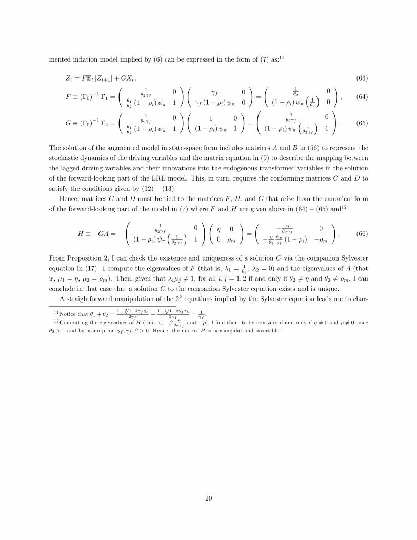
mented in�ation model implied by (6) can be expressed in the form of (7) as:11

Zt = FEt [Zt+1] +GXt; (63)

F � (�0)�1 �1 =

1�2 f

0�1�2(1� �i) � 1

! f 0

f (1� �i) � 0

!=

1�2

0

(1� �i) ��1�2

�0

!; (64)

G � (�0)�1 �2 =

1�2 f

0�1�2(1� �i) � 1

! 1 0

(1� �i) � 1

!=

0@ 1�2 f

0

(1� �i) ��

1�2 f

�1

1A : (65)

The solution of the augmented model in state-space form includes matrices A and B in (56) to represent the

stochastic dynamics of the driving variables and the matrix equation in (9) to describe the mapping between

the lagged driving variables and their innovations into the endogenous transformed variables in the solution

of the forward-looking part of the LRE model. This, in turn, requires the conforming matrices C and D to

satisfy the conditions given by (12)� (13).Hence, matrices C and D must be tied to the matrices F , H, and G that arise from the canonical form

of the forward-looking part of the model in (7) where F and H are given above in (64)� (65) and12

H � �GA = �

0@ 1�2 f

0

(1� �i) ��

1�2 f

�1

1A � 0

0 �m

!=

� ��2 f

0

� ��2

� f(1� �i) ��m

!: (66)

From Proposition 2, I can check the existence and uniqueness of a solution C via the companion Sylvester

equation in (17). I compute the eigenvalues of F (that is, �1 = 1�2, �2 = 0) and the eigenvalues of A (that

is, �1 = �, �2 = �m). Then, given that �i�j 6= 1, for all i; j = 1; 2 if and only if �2 6= � and �2 6= �m, I can

conclude in that case that a solution C to the companion Sylvester equation exists and is unique.

A straightforward manipulation of the 22 equations implied by the Sylvester equation leads me to char-

11Notice that �1 + �2 =1� 2p1�4 f b2 f

+1+ 2p1�4 f b2 f

= 1 f.

12Computing the eigenvalues of H (that is, �� ��2 f

and ��), I �nd them to be non-zero if and only if � 6= 0 and � 6= 0 since�2 > 1 and by assumption f ; f ; � > 0. Hence, the matrix H is nonsingular and invertible.

20

acterize the conforming matrices C and D as follows:13

C =

0@ 1 f

�1

�2��

�� 0

� (1� �i) 1 f

�1

�2��

�� �m

1A ; D � CA�1B =

0@ 1 f

�1

�2��

��� 0

� (1� �i) 1 f

�1

�2��

��� ��

1A : (67)

Checking Condition 2 is straightforward to see that rank (C) = 2 if and only if � 6= 0 and � 6= 0 since �2 > 1and by assumption f ; f > 0 and � > 1 (the Taylor principle). All of this, in turn, implies that there

exists a unique matrix C that solves the companion Sylvester equation in (17) and is also invertible. Hence,

the inverse of C is given as:

C�1 =

f (�2 � �) 1� 0

� � (1� �i) 1�m

1�m

!: (68)

Therefore, the forward-looking part of the augmented in�ation model has a VAR(1) representation in

the form of (16) which can be expressed as:

Zt = CAC�1Zt�1 + CA�1B�t; (69)

where

CAC�1 =

� 0

(� � �m) � (1� �i) �m

!; CA�1B =

0@ 1 f

�1

�2��

��� 0

� (1� �i) 1 f

�1

�2��

��� ��

1A : (70)

Then, the �nite-order VAR solution of the full-�edged LRE model in (19) becomes:

Wt = 1Wt�1 +2Wt�2 +3�t; (71)

13Using the properties of vectorization and the Kronecker product, I can write the companion Sylvester equation in simplelinear form as Avec (C) = vec (H) where:

A :=h�AT F

�� Ik2

i=

0BBBB@��2� 1 0 0 0

(1� �i) ����2

��1 0 0

0 0 �m�2

� 1 0

0 0 (1� �i) ���m�2

��1

1CCCCA :

From here it follows that:

vec (C) = A�1vec (H) =

0BBB@�2

���20 0 0

����2

(1� �i) � �1 0 0

0 0 � �2�2��m

0

0 0 � �m�2��m

(1� �i) � �1

1CCCA0BBB@

� ��2 f

� ��2

� f(1� �i)

0��m

1CCCA =

0BBB@�

f (�2��)�

f (�2��) � (1� �i)

0�m

1CCCAUndoing the vectorization, the solution C in (67) follows.

21

where

1 ���+ CAC�1

�=

� + �1 0

� (1� �i) (� + �1 � �m) �i + �m

!; (72)

2 � �CAC�1� =

���1 0

� � (1� �i) ��1 ��i�m

!; (73)

3 � CA�1B =

0@ 1 f

�1

�2��

��� 0

� (1� �i) 1 f

�1

�2��

��� ��

1A : (74)

From an economic point of view, the solution of the augmented model presented here indicates that there are

no spillovers from lagged interest rates into current in�ation. Spillovers are only from lagged in�ation into the

policy rate itself. The policy parameter � determines the magnitude of the spillovers from lagged in�ation

into the current policy rate� while the di¤erence in persistence across shocks (� + �1 � �m) in�uences thesign of the spillover from last period�s in�ation. Moreover, current monetary policy shocks do not contribute

to in�ation �uctuations. The policy parameter � plays a key role in explaining the contribution of the

monetary policy shock innovation relative to that of the real marginal shock innovation in accounting for

the policy rate volatility.

A Multivariate Model of In�ation. Monetary policy has no e¤ect on in�ation in the bivariate model

given by (42), (43), (51) and (52). This is because the exogenous process for real marginal costs alone drives

the dynamics of in�ation via the hybrid Phillips curve. In fact, the solution of in�ation is exactly the same

as that of the univariate case and could have been derived separately since there are no linkages built into

the model between the dynamics of in�ation and the policy. A further extension of the in�ation model that

gives monetary policy a distinct role in the determination of real marginal costs and in�ation is required. To

do so, I follow the approach underlying the workhorse three-equation New Keynesian model which partly

endogenizes the real marginal costs and connects them explicitly to monetary policy actions.

To be more precise, I retain the exogenous real marginal cost et in the hybrid Phillips curve equation but

augment the speci�cation in (42) with an endogenous real marginal cost component that is proportional to

the output gap yt, i.e.,

�t = fEt (�t+1) + b�t�1 + �yt + et; (75)

where the parameter � > 0 identi�es the slope of the hybrid Phillips curve. With external habit formation,

the household�s utility is a¤ected by aggregate consumption (Campbell and Cochrane (1999)). External

habits, therefore, lead the output gap yt to evolve according to the following hybrid dynamic IS equation:

yt = (1� h)Et (yt+1) + hyt�1 ��2h� 1�

�(it � Et (�t+1)� rnt ) ; (76)

where � > 0 determines the intertemporal elasticity of substitution and the coe¢ cient h � 0 introduces

external habit persistence in the speci�cation. Needless to say, whenever h = 0 equation (76) collapses to

the familiar time-separable dynamic IS equation. The natural rate rnt is assumed to follow an exogenously

given �rst-order autoregressive process:

rnt = #rnt�1 + ���t; (77)

22

where �t is assumed to be white noise with zero mean and variance of one, and uncorrelated at all leads

and lags with �t and �t. The persistence parameter �1 < # < 1 is expected to be less than one in absolute

value to ensure the stationarity of the process, while the parameter �� > 0 pins down the natural rate shock

volatility. Finally, I also modify the monetary policy rule in (51) as follows:

it = �iit�1 + (1� �i) [ ��t + yyt] +mt; (78)

to allow policy to respond to the endogenous output gap with the corresponding policy parameters set as

� > 1 and y > 0.14

Let me de�ne the vector of endogenous variables as Wt = (yt; �t; it)T , the driving variables as Xt =

(rnt ; et;mt)T , and the vector of innovations as �t = (�t; �t; �t)

T . The forward-looking part of the three-

equation New Keynesian model of in�ation given by (75), (76), and (78) can be expressed as:

D0Wt = D1Wt�1 +D2Et [Wt+1] +D3Xt; (79)

D0 =

0B@ 1 0�2h�1�

��� 1 0

� (1� �i) y � (1� �i) � 1

1CA ;

D1 =

0B@ h 0 0

0 b 0

0 0 �i

1CA ; D2 =

0B@ (1� h)�2h�1�

�0

0 f 0

0 0 0

1CA ; D3 =

0B@�2h�1�

�0 0

0 1 0

0 0 1

1CA ;

(80)

and re-written, whenever D0 is nonsingular, in the form of (1):

Wt = �1Wt�1 +�2Et [Wt+1] + �3Xt; (81)

�1 � (D0)�1D1; �2 � (D0)

�1D2; �3 � (D0)

�1D3: (82)

The shock processes in (43), (52), and (77) can be cast in the form indicated by the matrix equation (8)

with conforming matrices A and B given by:

A =

0B@ # 0 0

0 � 0

0 0 �m

1CA ; B =

0B@ �� 0 0

0 �� 0

0 0 ��

1CA : (83)

Then, the solution of the three-equation New Keynesian model can be derived following the steps of the

procedure proposed in this paper by solving a companion quadratic matrix equation and a companion

Sylvester equation.

In this case, I illustrate the solution of the full-�edged LRE model numerically taking advantage of the

set of Matlab codes and functions that I have written to implement the procedures described in this paper.15

14While the output gap may not be observable, one can rewrite the New Keynesian model in terms of the observable outputand a stochastic process for output potential. The output potential is driven by the same shock process as the natural rate,so the three-equation New Keynesian model can still be cast with three endogenous variables� all of them observable withoutput in place of the output gap� and three exogenous shock processes. A related illustration extending the workhorse NewKeynesian model (de�ned on observable output, in�ation and the policy rate) to a two-country setting can be found in Duncanand Martínez-García (2015).15 In terms of implementation, the solution of the full-�edged LRE model requires solving a quadratic matrix equation as in (5)

23

First, let me assume the parameters of the New Keynesian model speci�ed for this application take the

conventional parameterization presented in Table 1:

Table 1. Parameterization of the Three-Equation New Keynesian Model

Structural Parameter Notation Value

Forward-looking weight on Phillips curve f 0:7

Backward-looking weight on Phillips curve b 0:29

Slope of the Phillips curve � 0:5

Intertemporal elasticity of substitution � 1

External habit formation parameter h 0:6

Monetary Policy

Monetary policy inertia �i 0:85

Monetary policy response to in�ation deviations � 1:5

Monetary policy response to output gap deviations y 0:5

Exogenous Shock Parameters

Persistence of the natural interest rate shock # 0:95

Volatility of the natural interest rate shock �� 1

Persistence of the cost-push shock � 0:8

Volatility of the cost-push shock �� 2

Persistence of the monetary policy shock �m 0:3

Volatility of the monetary policy shock �� 0:7

The parameter values are chosen to illustrate the qualitative features of the three-equation New Keynesian

model and the performance of the algorithms for the solution of the companion quadratic matrix equation

and the companion Sylvester equation. I use a laptop with Intel(R) Core(TM) i7 with 2.7GHz, 4 cores and

32GB of installed memory (RAM). The wall-clock time elapsed in computing and reporting the numerical

given the defaults of the code is 0.150890 seconds (CPU time is: 0.1716 seconds). Using the iterative

algorithm to compute the solution to the quadratic matrix equation and Matlab�s own implementation of

the Hessenberg-Schur algorithm for Lyapunov equations to speed up the computation, the elapsed time falls

to 0.088264 seconds (CPU time is: 0.1248 seconds).

The code con�rms that, given the parameterization of Table 1, the solution � to the companion quadratic

matrix equation has its roots inside the unit circle. Furthermore, the code also reports that the solution C

to the companion Sylvester equation exists, and is both unique and invertible. Therefore, a straightforward

implementation of the algorithm implies that the the three-equation New Keynesian model has a �nite-

and a companion Sylvester equation as in (17). In the univariate and bivariate illustrations presented before, the solution of themodel can be achieved analytically with standard matrix algebra. However, the paper includes a straightforward Matlab codeimplementation to compute numerically the solution of the three-equation New Keynesian model via the companion quadraticmatrix equation in (5) and the companion Sylvester equation in (17). I use those codes in the rest of this section and madethem available in my website: https://sites.google.com/site/emg07uw/. The codes can be downloaded directly using this link:https://sites.google.com/site/emg07uw/econ�les/LRE_model_solution.zip?attredirects=0. Straightforward manipulations ofthose codes can be made to adapt them to other LRE models that can be cast in the canonical form investigated in thispaper� users of the codes are invited to include a citation of this paper in their work.The Matlab programs and functions appear free of errors, however I do appreciate all feedback, suggestions or corrections

that you may have. While users are free to copy, modify and use the code for their work, I do not assume any responsibilityfor any remaining errors or for how the codes may be used or misused by users other than myself.

24

order VAR(2) representation given by (19) under the parameterization reported in Table 1 which takes the

following form:

Wt = 1Wt�1 +2Wt�2 +3�t; (84)

1 =

0B@ 1:7257 �0:2344 0:0140

0:9303 0:6517 0:1666

0:3162 0:0616 1:1885

1CA ;

2 =

0B@ �0:7918 0:0567 0:0643

�0:8523 �0:1542 0:0417

�0:2512 �0:0305 �0:2408

1CA ;

3 =

0B@ 1:4816 0:0097 �0:83493:3205 3:8860 �1:71350:8582 0:8751 0:2518

1CA ;

(85)

where the corresponding coe¢ cient matrices 1 ���+ CAC�1

�, 2 � �CAC�1�, and 3 � CA�1B� for

standard parameterizations� have non-zero entries everywhere. This is in contrast with the bivariate model

presented where there were no spillovers from lagged interest rates to current in�ation.

From an economic perspective, the solution of the three-equation New Keynesian model shows that

there could be spillovers from lagged interest rates to in�ation whenever the real marginal costs are partly

endogenous and tied to short-term interest rate movements through a dynamic IS equation. Moreover,

monetary policy shocks in the full-�edged New Keynesian model contribute to drive the in�ation dynamics

unlike in the bivariate version of the model presented earlier. Given that the �nite-order VAR(2) solution of

the workhorse New Keynesian model exists, one may be able to identify the structural monetary policy shock

itself� as well as all other fundamental economic shocks driving the economy� directly from the observable

data.

The impact of monetary policy on the volatility, cyclicality and persistence of the endogenous variables

depends in nonlinear ways on the policy parameters, � and y, that describe the systematic part of

monetary policy. Here, I exploit the �nite-order VAR(2) representation to compute the theoretical moments

of the workhorse New Keynesian model for the benchmark parameterization of � and y, but also for

increasingly higher values of the anti-in�ation bias �. I summarize the key �ndings describing the business

25

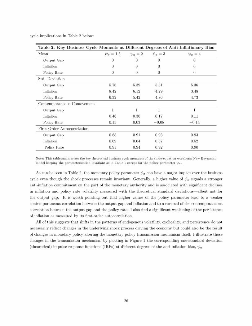
cycle implications in Table 2 below:

Table 2. Key Business Cycle Moments at Di¤erent Degrees of Anti-In�ationary Bias

Mean � = 1:5 � = 2 � = 3 � = 4

Output Gap 0 0 0 0

In�ation 0 0 0 0

Policy Rate 0 0 0 0

Std. Deviation

Output Gap 5:76 5:39 5:31 5:36

In�ation 8:42 6:12 4:29 3:48

Policy Rate 6:32 5:42 4:86 4:73

Contemporaneous Comovement

Output Gap 1 1 1 1

In�ation 0:46 0:30 0:17 0:11

Policy Rate 0:13 0:03 �0:08 �0:14First-Order Autocorrelation

Output Gap 0:88 0:91 0:93 0:93

In�ation 0:69 0:64 0:57 0:52

Policy Rate 0:95 0:94 0:92 0:90

Note: This table summarizes the key theoretical business cycle moments of the three-equation workhorse New Keynesianmodel keeping the parameterization invariant as in Table 1 except for the policy parameter � .

As can be seen in Table 2, the monetary policy parameter � can have a major impact over the business

cycle even though the shock processes remain invariant. Generally, a higher value of � signals a stronger

anti-in�ation commitment on the part of the monetary authority and is associated with signi�cant declines

in in�ation and policy rate volatility measured with the theoretical standard deviations� albeit not for

the output gap. It is worth pointing out that higher values of the policy parameter lead to a weaker

contemporaneous correlation between the output gap and in�ation and to a reversal of the contemporaneous

correlation between the output gap and the policy rate. I also �nd a signi�cant weakening of the persistence

of in�ation as measured by its �rst-order autocorrelation.

All of this suggests that shifts in the patterns of endogenous volatility, cyclicality, and persistence do not

necessarily re�ect changes in the underlying shock process driving the economy but could also be the result

of changes in monetary policy altering the monetary policy transmission mechanism itself. I illustrate those

changes in the transmission mechanism by plotting in Figure 1 the corresponding one-standard deviation

(theoretical) impulse response functions (IRFs) at di¤erent degrees of the anti-in�ation bias, �.

26

Figure 1. Theoretical IRFs at Di¤erent Degrees of Anti-In�ationary Bias

Note: This �gure displays the theoretical impulse response functions (IRFs) of the three-equation workhorse NewKeynesian model keeping the parameterization invariant as in Table 1 except for the policy parameter � .

I note that a higher anti-in�ation bias stance on monetary policy (" �) tends to dampen the impact onthe endogenous variables of cost-push and monetary policy shock innovations. However, while the impact

on in�ation of natural-rate shock innovations also declines, a higher � tends to amplify the e¤ect (at least

in the initial quarters) of those same innovations in the output gap and the policy rate.

Hence, these �ndings con�rm the view that identifying structural shocks� monetary policy shocks in

particular� is only part of the task, and that the transmission mechanism and its spillovers ultimately depend

in nonlinear ways on the features of the prevailing monetary policy regime� the policy parameters of the

Taylor (1993) rule in this case� and other deep structural parameters related to preferences, technology, etc.

Hence, the method proposed in this paper to solve canonical LRE models makes an important contribution

to help us understand the transmission mechanism in a large class of macro models and its mapping into

�nite-order VAR speci�cations.

5 Concluding Remarks

I propose a novel approach to solve a large class of LRE models. I represent the LRE model in its canonical

form as a system of expectational �rst-order di¤erence equations. Then, I reduce the canonical form by

splitting the backward-looking and forward-looking parts of the model via the solution of a companion

quadratic matrix equation (Binder and Pesaran (1995, 1997)). The forward-looking part is solved through

the method of undetermined coe¢ cients and describes the unique solution� when one exists� by means of

a linear state-space model. Finally, I check the existence and uniqueness of a solution to the purely forward-

looking part of the LRE model and characterize its corresponding reduced-form solution in �nite-order VAR

27

form via a companion Sylvester equation.

An important contribution of the paper is the derivation of conditions under which the reduced-form,

�nite-order VAR solution of the forward-looking part of the LRE model via the well-known Sylvester matrix

equation is well-de�ned. The approach proposed in the paper not only provides a way to decouple the

canonical form of the LRE model and to characterize the solution in �nite-order VAR form, but also checks

its properties� existence, uniqueness and invertibility. Furthermore, the paper also makes a contribution to

the existing computation literature with the development of an integrated algorithm to solve computationally

for models for which a unique �nite-order VAR representation exists.

Solving LRE models with a VAR representation by this method is straightforward to implement, e¢ cient,

and can be handled easily with standard matrix algebra and conventional computational methods. The

paper provides a number of functions for the solution of the companion quadratic matrix equation and the

companion Sylvester equation with an economically-relevant application to the study of the transmission

mechanism of monetary policy. For this purpose, the paper provides an illustration of the procedure based

on the workhorse New Keynesian model and discusses the fundamental features of the model that permit

the propagation of monetary policy shocks to in�ation and the output gap� with particular attention to

the role of the systematic part of the monetary policy rule (which determines the response to in�ation and

output deviations from their targets). The paper also points out how under the conditions that ensure the

existence of a �nite-order VAR representation of the solution, the identi�cation of fundamental shocks for

empirical research� including the identi�cation of monetary shocks� can be made tractable.

References

[1] Anderson, E. W., McGrattan, E. R., Hansen, L. P. and Sargent, T. J. (1996): "Mechanics of Forming

and Estimating Dynamic Linear Economies." Handbook of Computational Economics, Vol. 1, pp.

171-252. Elsevier Science, Amsterdam.

[2] Bartels, R. H. and Stewart, G. W. (1972): "Algorithm 432: Solution of the matrix equation AX+XB =

C." Comm. ACM, 15 (9), pp. 820-826.

[3] Binder, M. and Pesaran, M. H. (1995): "Multivariate Rational Expectations Models and Macroeconomic

Modelling: A Review and Some New Results," in Pesaran, M. H. and Wickens, M. (eds.), Handbook

of Applied Econometrics: Macroeconomics, pp. 139-187.

[4] Binder, M. and Pesaran, M. H. (1997): "Multivariate Linear Rational Expectations Models: Char-

acterization of the Nature of the Solutions and Their Fully Recursive Computation." Econometric

Theory, Vol. 13 (6), pp. 877-888.

[5] Blanchard, O. J. and Kahn, C. M. (1980): "The Solution of Linear Di¤erence Models Under Rational

Expectations." Econometrica, Vol. 48 (5), pp. 1305-1311.

[6] Broze, L., Gouriéroux, C. and Szafarz, A. (1985): "Solutions of Dynamic Linear Rational Expectations

Models." Econometric Theory, Vol. 1, pp. 341-368.

[7] Broze, L., Gouriéroux, C. and Szafarz, A. (1990): "Reduced Forms of Rational Expectations Models."

Chur, Switzerland: Harwood Academic Publishers.

28

[8] Calvo, G. A. (1983): "Staggered Prices in a Utility-Maximizing Framework". Journal of Monetary

Economics, Vol. 12 (3), pp. 383-398.

[9] Campbell, H. and Cochrane, J. (1999): "By Force of Habit: A Consumption-Based Explanation of

Aggregate Stock Market Behavior." Journal of Political Economy, Vol. 107 (2), pp. 205-251.

[10] Christiano, L. J. (2002): "Solving Dynamic Equilibrium Models by a Method of Undetermined Coe¢ -

cients." Computational Economics, Vol. 20 (1), pp. 21-55.

[11] Duncan, R. and Martínez-García, E. (2015): "Forecasting Local In�ation with Global In�ation: When

Economic Theory Meets the Facts." Globalization and Monetary Policy Institute Working Paper

No. 235, 2015.

[12] Fernández-Villaverde, J., Rubio-Ramírez, J., Sargent, T. and Watson, M. (2007): "ABCs (and Ds) of

Understanding VARs." American Economic Review, 97 (3), pp. 1021-1026.

[13] Franchi, M. and Paruolo, P. (2015): "Minimality of State Space Solutions of DSGEModels and Existence

Conditions for Their VAR Representation." Computational Economics, Vol. 46, pp. 613-626.

[14] Golub, G. H., Nash, S. and van Loan, C. F. (1979): "A Hessenberg-Schur Method for the Problem

AX +XB = C." IEEE Trans. Automat. Control, AC-24(6), pp. 909-913.

[15] Golub, G. H. and van Loan, C. F. (1996): "The Hessenberg and Real Schur Forms." in Matrix Compu-

tations, 3rd ed. Baltimore, MD: Johns Hopkins University Press, pp. 361-372.

[16] Hansen, L. and Sargent, T. (1980): "Formulating and Estimating Dynamic Linear Rational Expectations

Models." Journal of Economic Dynamics and Control, Vol. 2, pp. 7-46.

[17] Horn, R. A. and Johnson, C. R. (1991): "Topics in Matrix Analysis." Cambridge University Press.

[18] Inoue, A. and Kilian, L. (2002): "Bootstrapping Smooth Functions of Slope Parameters and Innovation

Variances in VAR(1) Models." International Economic Review, Vol. 43 (2), pp. 309-332.

[19] Jiang, T. and Wei, M. (2003): "On Solutions of the Matrix Equations X �AXB = C and X �AXB =C." Linear Algebra and Its Applications, Vol. 367, pp. 225-233.

[20] King, R. G. and Watson, M. W. (1998): "The Solution of Singular Linear Di¤erence Systems Under

Rational Expectations." International Economic Review, Vol. 39 (4), pp. 1015-1026.

[21] Klein, P. (2000): "Using the Generalized Schur Form to Solve a Multivariate Linear Rational Expecta-

tions Model." Journal of Economic Dynamics and Control, Vol. 24 (10), pp. 1405-1423.

[22] Lancaster, P. and Tismenetsky, M. (1985): "The Theory of Matrices with Applications. Second Ed."

Academic Press, New York.

[23] Lin, M. and Wimmer, H. K. (2011): "The Generalized Sylvester Matrix Equation, Rank Minimization

and Roth�s Equivalence Theorem." Bulletin of the Australian Mathematical Society, Vol. 84, pp.

441-443.

[24] Lubik, T. A. and Schorfheide, F. (2003): "Computing Sunspot Equilibria in Linear Rational Expecta-

tions Models." Journal of Economic Dynamics and Control, Vol. 28 (2), pp. 273-285.

[25] Lucas, R. (1976): "Econometric Policy Evaluation: A Critique." Carnegie-Rochester Conference Series

on Public Policy, Vol. 1, pp. 19-46.

29

[26] Muth, J. (1961): "Rational Expectations and the Theory of Price Movements." Econometrica, Vol. 29

(3), pp. 315-335.

[27] Ravenna, F. (2007): "Vector Autoregressions and Reduced Form Representations of DSGE Models."

Journal of Monetary Economics, Vol. 54, pp. 2048-2064.

[28] Sargent, T. (1980): "Rational Expectations and the Reconstruction of Macroeconomics." Federal Re-

serve Bank of Minneapolis Quarterly Review, Summer 1980, pp. 15-19.

[29] Sima, V. and Benner, P. (2015): "Solving Linear Matrix Equations with SLICOT." National Institute

for Research and Development in Informatics, Bucharest, Romania.

[30] Sims, C. A. (2002): "Solving Linear Rational Expectations Models." Computational Economics, Vol.

20 (1), pp. 1-20.

[31] Taylor, J. B. (1993): "Discretion versus Policy Rules in Practice". Carnegie-Rochester Conference Series,

Vol. 39, pp. 195-214.

[32] Uhlig, H. (1999): "A Toolkit for Analyzing Nonlinear Dynamic Stochastic Models Easily." in R. Marimon

and A. Scott: Computational Methods for the Study of Dynamic Economies. Oxford and New York:

Oxford University Press, 1999, pp. 30-61.

[33] Yun, T. (1996): "Nominal Price Rigidity, Money Supply Endogeneity, and Business Cycles." Journal

of Monetary Economics, Vol. 37 (2), pp. 345-370.

30

Appendix

A The LRE Model: From General Form to Canonical Form

The general form of a large class of multivariate LRE models can be written as

�00Yt =Xm

i=1�i0Yt�i +

Xm

i=0

Xn

j=1�ijEt�i (Yt+j�i) + et; (86)

where Yt and Xt are the r � 1 vectors of the endogenous and driving variables of the model, �ij for alli = 0; :::;m and j = 0; :::; n and are r � r conforming matrices, and Et (�) represents the conditionalexpectations operator based on all current and lagged values of Yt and et. I assume that �00 in (86) is

nonsingular and, without loss of generality, set it equal to the identity matrix Ir.

As in Broze et al. (1985, 1990) and Binder and Pesaran (1995, 1997), the canonical form of (86) is given

by

Wt = �1Wt�1 +�2Et [Wt+1] +Xt; (87)

where

Wt =�Y Tt ; Y

Tt�1; :::; Y

Tt�m+1

�T; UTt =

�Y Tt ;Et

�Y Tt+1

�; :::;Et

�Y Tt+n

��T;

�1 = �D�10 D1; �2 = �D�1

0 D1;

Xt = D�10 ut; ut =

�uTt ; 0

Tq�1; :::; 0

Tq�1�T; ut =

�(et)

T; 0Tr�1; :::; 0

Tr�1

�T;

where ut is a column-vector of dimension k = m (n+ 1) r and ut is a column-vector of dimension l = (n+ 1) r.

The k � k square matrices Di, i = �1; 0; 1 are de�ned as

D�1 =

0BBBB@�1 0l ::: 0l

0l 0l ::: 0l. . .

0l 0l ::: 0l

1CCCCA ;

D0 =

0BBBB@0 1 ::: m�1

0l Il ::: 0l. . .

0l 0l ::: Il

1CCCCA ;

D1 =

0BBBB@0l 0l ::: 0l m

�Il 0l ::: 0l 0l. . .

0l 0l ::: �Il 0l

1CCCCA ;

31

where i, i = �1; 0; :::;m are square matrices of dimension l given by

�1 =

0BBBB@0r 0r ::: 0r 0r

�Ir 0r ::: 0r 0r. . .

0r 0r ::: �Ir 0r

1CCCCA ;

0 =

0BBBB@Ir �A01 ::: �A0n0r Ir ::: 0r

. . .

0r 0r ::: Ir

1CCCCA ;

i =

0BBBB@�Ai0 �Ai1 ::: �Ain0r 0r ::: 0r

. . .

0r 0r ::: 0r

1CCCCA for i = �1; 0; :::;m:

The quadratic determinantal equation method of Pesaran and Binder (1995, 1997) deals with the simul-

taneous dependence of Wt on its past and its future expected values by transforming the canonical system

in (87) so that the resulting system in terms of the transformed variables contains only forward-looking and

not backward-looking terms of the transformed variables.

B The Moving Average Representation of the LRE Model

The canonical state-space representation of a large class of linear (and linearized) rational expectations

models can be given as in (8) � (9). With the assumption that all are square matrices, it follows fromequation (8) that [Ik �AL]Xt = B�t where Ik is a conforming identity matrix of dimension k and L is

the lag operator. If the eigenvalues of A are less than one in modulus, the solution has a moving average

representation. In that case, Xt becomes a square summable polynomial given by Xt =X1

j=0[A]

jB�t�j ;

this can be shifted one period back and replaced in (9) to obtain Zt = CX1

j=0[A]

jB�t�1�j +D�t.

The moving average representation implied by the state-space solution in (8)� (9) can be inverted undera simple condition and, therefore, represented with a VAR(1). Whenever the matrix D is nonsingular,

replacing the vector �t in (8) using (9) gives�Ik �

�A�BD�1C

�L�Xt = BD�1Zt: (88)

As noted in Fernández-Villaverde et al. (2007), if the eigenvalues of A�BD�1C are strictly less than one in

modulus, the inverse of the operator on the left-hand side of (88) gives Xt as a square summable polynomial

in L satisfying

Xt =X1

j=0

�A�BD�1C

�jBD�1Zt�j : (89)

32

Shifting this expression back one period and replacing it in (9), I obtain

Zt = CX1

j=0

�A�BD�1C

�jBD�1Zt�1�j +D�t: (90)

In general, the VAR(1) representation of the solution can be reasonably well-approximated by a �nite-orderstructural VAR model as shown in Inoue and Kilian (2002).

In this paper, my methodological contribution is twofold: I propose a new approach to derive the state-

space solution in (8) � (9) from the solution of a companion Sylvester equation and a testable condition

under which a �nite-order VAR representation will be exact rather than an approximation for the LRE

model solution. The method proposed here is very e¢ cient at computing the solution to a large class of

LRE models. It also checks a straightforward condition� the invertibility of the solution to the companion

Sylvester equation� and e¢ ciently derives the corresponding �nite-order VAR representation of the solution

to the canonical LRE model when one exists.

C An Algorithm to Solve the Quadratic Matrix Equation

Binder and Pesaran (1995, 1997) solve the quadratic matrix equation in (5) for its (stable) real-valued

solution � with a straightforward iterative algorithm.16 Alternatively, I look for the stable solution of the

quadratic matrix equation in (5) via a companion matrix form where the k � k matrices �1 and �2 that

describe the quadratic matrix equation enter into the following 2k � 2k matrices

D =

"Ik ��1Ik 0k

#; E =

"�2 0k

0k Ik

#: (91)

The solution to the generalized eigenvalue problem for the matrix pair (D;E) is a set of 2k eigenvalues qk and

their corresponding eigenvectors vk such that Dvk = Evkqk. Assuming there are at least k stable eigenvalues

(those who are inside the unit circle), I can then order the eigenvalues and corresponding eigenvectors so

that the k stable eigenvalues come �rst. Partitioning the ordered matrix of eigenvalues Q and the matrix

of eigenvectors V accordingly, i.e. Q =

"Q1 0k

0k Q2

#and V =

"V 11 V 12

V 21 V 22

#where each block matrix is of

dimension k � k, the generalized eigenvalue problem can be stated in matrix form as"Ik ��1Ik 0k

#"V 11 V 12

V 21 V 22

#=

"�2 0k

0k Ik

#"V 11 V 12

V 21 V 22

#"Q1 0k

0k Q2

#; (92)

and from here it follows that"V 11 � �1V 21 V 12 � �1V 22

V 11 V 12

#=

"�2V

11 �2V12

V 21 V 22

#"Q1 0k

0k Q2

#=

"�2V

11Q1 �2V12Q2

V 21Q1 V 22Q2

#: (93)

16The accompanying codes provided with the paper include a Matlab function that implements the iterative solution ofBinder and Pesaran (1995, 1995) together with the Matlab function that recovers the solution using alternatively the generalizedeigenvalue problem algorithm described in this Appendix. For a discussion of the quadratic matrix equation and the iterativealgorithm, the interested reader is also refered to Binder and Pesaran (1995, 1997) and the accompanying Matlab codes forreference: https://ideas.repec.org/c/dge/qmrbcd/73.html.

33

This block system implies that V 11 = V 21Q1 and V 11��1V 21 = �2V 11Q1. Substituting the �rst expressioninto the second one gives that V 21Q1��1V 21 = �2V 21Q1Q1; then, post-multiplying both sides by

�V 21

��1and re-arranging, it follows that:

�2

�V 21

�Q1�2 �

V 21��1�� �V 21Q1 �V 21��1�+�1 = 0k: (94)

De�ning � to be � � V 21Q1�V 21

��1gives �2 = V 21Q1

�V 21

��1V 21Q1

�V 21

��1= V 21

�Q1�2 �

V 21��1

.

Therefore, under this de�nition of �, the expression above is observationally equivalent to the quadratic

matrix equation in (5). This su¢ ces to characterize a solution of the quadratic matrix equation based on its

k stable eigenvalues.

If such a real-valued solution of the quadratic matrix equation exists with all its eigenvalues inside the

unit circle, then it is straightforward to compute by constructing the matrices D and E and �nding the

ordered solution to the corresponding generalized eigenvalue problem for those matrices. The block matrix

Q1 contains the k stable eigenvalues and the block matrix V 21 contains the corresponding eigenvectors from

the generalized eigenvalue problem after partitioning, then I can construct the solution � for the quadratic

matrix simply as � � V 21Q1�V 21

��1.

34