Working Paper

WP No 560

May, 2004

MANAGING CUSTOMER RELATIONSHIPS: SHOULD MANAGERS REALLY FOCUS ON THE LONG TERM?

Julian Villanueva * Pradeep Bhardwaj **

Yuxin Chen *** Sridhar Balasubramanian ****

* Professor of Marketing, IESE ** The Anderson School of at UCLA ** Leonard N. Stern School of Business, New York University **** Kenan-Flagler Business School, University of North Carolina at Chapel Hill

IESE Business School – Universidad de Navarra Avda. Pearson, 21 – 08034 Barcelona. Tel.: (+34) 93 253 42 00 Fax: (+34) 93 253 43 43 Camino del Cerro del Águla, 3 (Ctra. de Castilla, km. 5,180 – 28023 Madrid. Tel.: (+34) 91 357 08 09 Fax: (+34) 91 357 29 13

Copyright © 2004 IESE Business School. Do not quote or reproduce without permission

MANAGING CUSTOMER RELATIONSHIPS: SHOULD MANAGERS REALLY FOCUS ON THE LONG TERM?

Abstract

Researchers and business thought leaders have emphasized that, towards

maximizing the lifetime value of customers, firms must manage customer relationships for the long term. In contrast to this recommendation, we demonstrate that firm profits in competitive environments are maximized when managers focus on the short term with respect to their customers. Intuitively, while a long term focus yields more loyal customers, it sharpens short term competition to gain and keep customers to such an extent that overall firm profits are lower than when managers focus on the short term. Further, a short term focus continues to deliver higher profits even when customer loyalty yields a higher share-of-wallet or reduced costs of service from the perspective of the firm. Intuitively, while such revenue enhancement or cost reduction effects enhance the proverbial pot of gold at the end of the rainbow, they lead to even more intense competition to gain and keep customers in the short term. These findings suggest that the competitive implications of a switch to a long term customer focus must be carefully examined before such a switch is advocated or implemented. Paradoxically, customer lifetime value may be maximized when managers focus on the short term.

Keywords: targeted pricing, customer equity, price discrimination, customer relationship marketing, customer acquisition, customer retention

MANAGING CUSTOMER RELATIONSHIPS: SHOULD MANAGERS REALLY FOCUS ON THE LONG TERM?

Introduction

A stable customer base increases the value of the firm to its owners. Accordingly,

researchers and business thought leaders have held that firms must manage their customers for the long term in order to maximize customer lifetime value (CLV, henceforth) (e.g., Blattberg and Deighton 1996; Blattberg, Getz, and Thomas 2001; Rust, Zeithaml, and Lemon 2000; Winer 2001). This view has guided recent initiatives related to customer relationship management (CRM).

In this paper, we ask whether marketing managers in the field must really focus on the long term with respect to their customers. Our surprising answer is that overall firm profits are higher in competitive environments when their managers maximize short term profits from customers. Specifically, we demonstrate using a game theoretic framework that rotating managers in charge of the customer base so that each manager is focused only on short term profits yields higher overall profits than when managers focus on the long term. While a long term strategy leads to more loyal customers, it also intensifies the competition to gain and keep customers. This increase in short term competition can swamp the gains from a long term focus. Paradoxically, therefore, CLV may be maximized when managers focus on the short term.

To demonstrate these results, we develop an analytical model of behavior-based pricing. Two firms compete over two periods, and each firm is endowed with a customer at the beginning of the game. Firms can offer individualized prices to customers. Ex ante, customers have identical switching costs, but in any given period a particular customer is in a “variety seeking” mode (i.e., the customer is a potential switcher) with a certain probability. Customers who switch firms incur a switching cost. Firms are aware of the magnitude of the switching cost but do not know whether a specific customer is in a variety-seeking mode. These assumptions are designed to capture the randomness of switching behavior and the inability of firms to accurately gauge a specific customer’s propensity to switch—these are significant practical challenges faced by managers in the field. Firms can decide, using organizational arrangements or otherwise, whether their managers focus on short term or long term profits.1

1 It is well known that acquiring customers is expensive compared to serving existing customers. In the context of the model, this situation can be captured by a high switching cost.

2

Our central focus is on a comparison of the two (symmetric) regimes that result when managers focus on either the short or the long term. In the first regime, managers in both firms are focused on the long term and act to directly maximize the lifetime value of customers (the resulting equilibrium is denoted by CLV-CLV). In the second regime, managers in both firms are rotated between periods so that each manager maximizes per-period profits (this equilibrium is denoted by ST-ST). We find that overall firm profits under ST-ST are, in striking contrast to received wisdom, always higher than those under CLV-CLV.2

Interestingly, while scholars and business leaders have recommended a long term focus with respect to customers, managers in the field are often myopic on account of career concerns or pressures from external entities, including the stock market. Consider these illustrations:

– “At any given time, more than 40% of managers and senior executives expect to leave their jobs within two years” (Business Week, June 6, 2002).

– When managers have mobility within the labor market, they tend to make decisions that yield short-term gains at the expense of long-term interests of shareholders. This incentive arises because these managers seek to boost their reputation earlier, thereby boosting wages (Narayanan 1985).

– A participant in a CFO conference noted that the focus would shift from making the quarterly numbers to overall business health only “When and if the public and analysts start to take a more visionary and longer term look at companies, and stock prices stop being volatile based on quarterly earnings…” (CFO Magazine, June 26, 2002).

– A financial expert commented on the pressure to manage short-term earnings: “… if you were to speak to any chief executive of a public company anywhere in the world, or a CFO as well who deals with institutional investors on a day-to-day basis, they are all hide-bound these days by the requirement to have growth every quarter” (ABC Radio National Australia Report, Feb. 8, 2003).

Our findings suggest that this short term focus commonly encountered in the field can yield some unexpected benefits. However, our basic analysis does not accommodate the argument that long lived customers are typically more profitable, either because they tend to spend more with the firm (a “revenue expansion” effect) or because they are less costly to serve (a “cost reduction” effect). Ostensibly, cultivating customers with an eye on the long term would be more profitable here. We demonstrate that this argument is not necessarily correct. While these effects do enhance the proverbial pot of gold at the end of the rainbow, they also increase the intensity of short run competition to gain and keep customers. Correspondingly, profits under ST-ST remain higher than under CLV-CLV even when such effects apply.3

In §2, we describe related work. The basic model is presented in §3. The equilibria that result when each firm can choose between a CLV and ST focus for its managers are analyzed in §4. Revenue expansion and cost reduction effects are examined in §5. We conclude with §6.

2 For technical completeness, we also demonstrate that CLV-ST does not constitute an equilibrium strategy pairing.

3 Reinartz and Kumar (2000, 2002) discuss why loyal customers may not be profitable for non-strategic reasons.

3

Background

The question of whether firms should act to maximize customer lifetime value in competitive environments has not yet been theoretically addressed. However, related research that has viewed competition through the lens of the customer has focused on how competitive outcomes are influenced by a) the presence of “loyal” and “switcher” segments, b) switching costs, and c) targeted prices and promotions.

A first stream of literature has examined how the size and behavior of loyal and switcher segments affect competitive outcomes. In markets with a switcher segment, the equilibrium frequently involves mixed strategies, i.e., competing firms may choose from a distribution of prices, with the average price for the firm with the larger (absolute) share of loyals higher than that of the competitor (Narasimhan 1988). Accordingly, the periodic discounts encountered in competitive marketplaces may be interpreted as prices that fall below the upper limit of the distribution. When firms can convert a fraction of first-time buyers into loyals by providing a certain level of service, a firm with an initially large customer base will typically provide higher levels of service (McGahan and Ghemawat 1994). This ensures that the smaller firm, which gains more from price undercutting when price is the only strategic variable, instead provides lower service levels and focuses on attracting switchers.

A second stream of literature has focused on how “switching costs,” i.e., the incremental costs that customers incur in shifting between sellers, influence competition (e.g., von Weizsacker 1984, Klemperer 1987a, 1987b). When firms compete over multiple periods, such costs may lessen long run competition because the “locked-in” customers are less price sensitive. However, anticipating the resulting higher profits, firms compete more strongly to attract customers in the earlier periods—overall, firms may not be better off (Klemperer 1987a). When customers can foretell that the firm with the larger market share will charge higher future prices, they are less sensitive to early price differences. Hence, firms may compete less even in the first stage compared to an identical market without switching costs (Klemperer 1987b).4

Switching costs can also lead to a temporary price war when a new seller enters a market. Here, the entrant will price low and the incumbent’s price will also fall during entry, but once the customers are locked-in, prices rise (Klemperer 1989). Therefore, a market with switching costs may be more attractive to an entrant when long run profits are considered. In general, markets with switching costs are more profitable than those without, even when new customers arrive and some existing customers leave each period (Beggs and Klemperer 1992, Klemperer 1995).5

A third related stream of literature has examined how competition is influenced by coupons or differential prices that are targeted at individual customers. Modern developments in information technology have enabled more of such “behavior-based” discrimination, where marketing initiatives are targeted at buyers on the basis of observed behaviors. An interesting early finding in this context was that, while random coupon drops (i.e., “mass-media” coupons) raise prices and profits in a competitive environment, coupon drops targeted specifically at brand switchers lead to lower profits (Shaffer and Zhang 1995). Intuitively, competitors closely match couponing activity when coupons are targeted, yielding a prisoner’s dilemma where each firm’s profits are reduced by the sum of the cost of distributing the coupons and their face value.

4 When products are perfect substitutes, switching costs can result in all-or-nothing results—e.g., in overlapping generations models, firms may alternate between selling to all of the new and all of the old customers (Farrell and Shapiro 1988; Padilla 1992).

5 Klemperer (1995) analyses the competitive implications of switching costs in industrial organization, macroeconomic, and international trade contexts.

4

When firms that compete over an infinite horizon with overlapping generations of customers can recognize and target their own customers with a different price (but not differentiate between new and existing customers of competitors), steady-state prices depend on three factors (Villas-Boas 1999). First, firms poach each other’s customers in equilibrium—this lowers prices. Second, prices are lower when customers are patient. Such patience sensitizes customers to current prices in any period, thereby increasing the intensity of price competition. Finally, firms recognize that owning a large customer base will intensify future price competition as the competitors will aggressively poach that clientele—this reduces current price competition.

Much of the existing literature demonstrates that one-to-one promotions and reward programs targeted at specific customers do not pay off in terms of increased profits and instead lead to a prisoner’s dilemma (e.g., Chen 1997; Fudenberg and Tirole 2000; Kopalle and Neslin 2003; Shaffer and Zhang 1995). However, those findings may be contingent on the assumptions that (a) all customers can potentially switch, and (b) the firms are symmetric. When a firm can correctly classify its own loyal customers and switchers only with a certain degree of probability (i.e., individual marketing is feasible, but imperfect), individual marketing can be profitable (Chen, Narasimhan, and Zhang 2001). Intuitively, since some price-sensitive switchers are mistaken to be price-insensitive loyals and receive a higher price, the competitor can attract them without lowering prices significantly—this softens price competition and supports higher profits. Likewise, when firms are differently sized, such promotions may reduce prices but yet be profitable on account of market share gains for the larger firm (Shaffer and Zhang 2002). Similarly, coupons and reward programs tend to be profitable when they expand the market rather than cull market share from competitors (Kopalle and Neslin 2003).

The specific issue of whether firms should adopt a long term focus with respect to their customers has yet to be addressed. For many firms, a long term customer focus may call for significant alterations in existing business strategy, operational processes, and compensation patterns. Before undertaking such a shift, a rigorous examination of its implications for firm profits is in order. We undertake such an examination in this paper.

The model

We study competition over two periods in a duopoly. Each firm “owns” one customer at the outset of period 1. Each customer has a reservation utility of 1 and buys at most one unit of the product in each period. In any period, each customer is a potential switcher with probability z — however, switching occurs only when the price difference between the firms is larger thanγ ( )1<γ . Here, z may be interpreted as a variety-seeking tendency and γ as a “switching cost.” Firms do not know whether a specific customer is in variety seeking mode. Marginal costs, fixed costs and the discount rate are set to zero. Firms offer prices to customers that could vary depending on whether a customer currently is with the firm or its competitor, i.e., prices can be targeted at zero cost. Customers purchase from the firm that offers them the highest utility.

The game sequence is as follows. At the outset of period 1, each firm “owns” one customer. Further, the owners of each firm decide whether their managers adopt either short-term, i.e. period-by-period, profit maximization (denoted by ST) or long-term profit maximization that maximizes the sum of the profits across the two periods (denoted by CLV). Next, each firm offers two prices, one for its own customer and the other for the competitor’s customer. Customers purchase from the firm that offers them the highest (positive) utility, possibly switching firms in the process. In period 2, each firm again offers

5

two prices, one for its own customer and the other for the competitor’s customer. Customers again make choices on observing these prices.

We first analyze a single-period game to set up a benchmark case—here, CLV or ST yield identical outcomes. The benchmark case also helps clarify the mechanics of the model.

1. Benchmark case (One period model)

Each firm begins the period with a customer. Denote firm 1’s profit from its customer during the period as Aπ and firm 2’s profit from the same customer as Bπ . Let prices offered to this customer of firm A by the two firms be Ap and Bp , respectively. Now, if firm 1 charged a price of 1 (the reservation utility), it is guaranteed a profit of (1 – z), which is the probability that the customer is a non-switcher. Therefore, firm 1 will not price below ( )z−1 , because expected profits from the customer would always be below the guaranteed profits for such a price. Firm 2 will not charge below 0, its marginal cost. Figure 1 describes the range of these prices.6

We assume that there is always a positive likelihood of customer “churn” in equilibrium—this case is both more practically relevant and more theoretically interesting.7 The condition that ensures a positive probability of switching is γ+> BA pp , i.e., the differences in prices charged by the firms must exceed the switching cost. Now, note that the lower limit of firm 1’s price is (1-z)—for any price higher than this, the likelihood that the condition γ+> BA pp holds is higher. If (1-z)<γ , then a pure strategy equilibrium exists. Here, firm 1 will price at infinitesimally below γ (which is greater than the lower limit 1-z) and keep the customer for sure with a resulting profit of γ , while firm 2 prices at 0, does not attract the customer, and obtains zero profits.

Figure 1

We focus on the case that is more interesting from theoretical and practical viewpoints, i.e., where (1-z)>γ (Figure 1 above). Note that: (a) If γ−−> zpB 1 , firm 1 has an incentive to undercut Bp so that γ+< BA pp (in this case, Ap remains above its lower limit 1-z); (b) if γ−−≤ zpB 1 , firm 1 has an incentive to raise Ap to 1 (because firm 1 can gain a higher profit by pricing on 1 and hoping for the outcome that the customer is a non-switcher); and (c) if γ>Ap , firm 2 has an incentive to undercut Ap by γ . Hence no pair of prices can constitute a pure-strategy equilibrium here—the potential for either undercutting the competitor (for both firms) or moving to the upper limit of price (in the case of firm 1) always exists.

6 It is not necessary to separately focus on the customer who begins with firm B at the outset of period 1. We will draw on the symmetry of the game to establish equilibrium outcomes related to that customer.

7 If a positive probability of long-run switching did not exist in equilibrium, each firm would be essentially a quasi-monopoly with respect to its own customer.

1-z

PA PB

γ1-zγ-γ

6

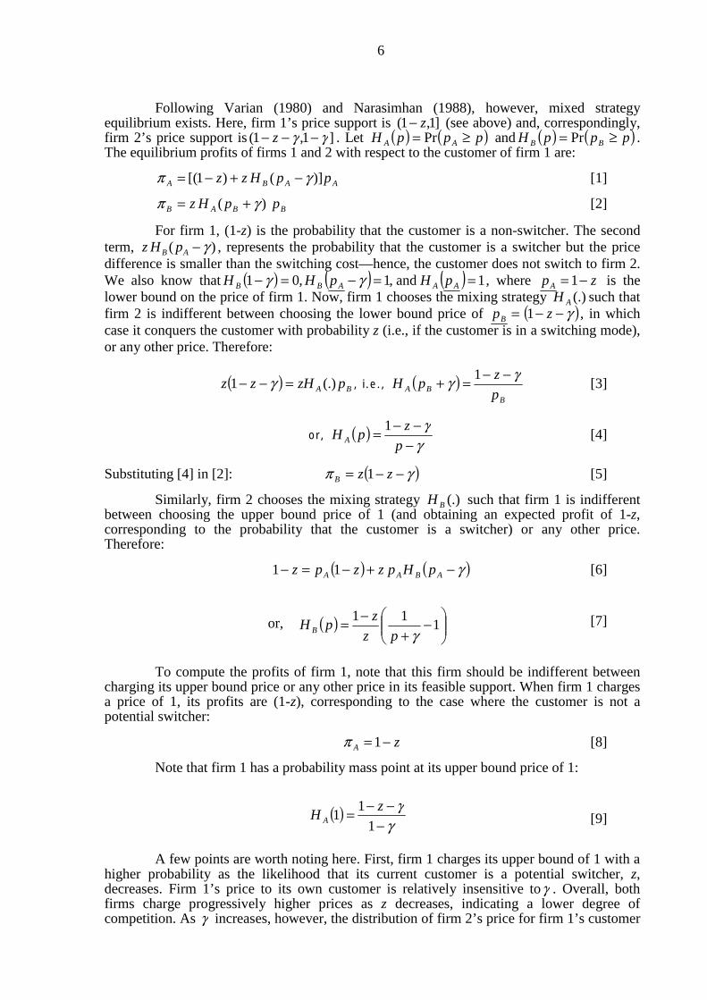
Following Varian (1980) and Narasimhan (1988), however, mixed strategy equilibrium exists. Here, firm 1’s price support is ]1,1( z− (see above) and, correspondingly, firm 2’s price support is ]1,1( γγ −−− z . Let ( ) ( )pppH AA ≥= Pr and ( ) ( )pppH BB ≥= Pr . The equilibrium profits of firms 1 and 2 with respect to the customer of firm 1 are:

AABA ppHzz )]()1[( γπ −+−= [1]

BBAB ppHz )( γπ += [2]

For firm 1, (1-z) is the probability that the customer is a non-switcher. The second term, )( γ−AB pHz , represents the probability that the customer is a switcher but the price difference is smaller than the switching cost—hence, the customer does not switch to firm 2. We also know that ( ) ( ) ( ) 1 and,1,01 ==−=− AAABB pHpHH γγ , where zpA −= 1 is the lower bound on the price of firm 1. Now, firm 1 chooses the mixing strategy (.)AH such that firm 2 is indifferent between choosing the lower bound price of =Bp ( )γ−− z1 , in which case it conquers the customer with probability z (i.e., if the customer is in a switching mode), or any other price. Therefore:

( ) BA pzHzz (.)1 =−− γ , i.e., ( )B

BA p

zpH

γγ −−=+ 1 [3]

or, ( )γ

γ−

−−=p

zpH A

1 [4]

Substituting [4] in [2]: ( )γπ −−= zzB 1 [5]

Similarly, firm 2 chooses the mixing strategy (.)BH such that firm 1 is indifferent between choosing the upper bound price of 1 (and obtaining an expected profit of 1-z, corresponding to the probability that the customer is a switcher) or any other price. Therefore:

( ) ( )γ−+−=− ABAA pHpzzpz 11 [6]

or, [7]

To compute the profits of firm 1, note that this firm should be indifferent between charging its upper bound price or any other price in its feasible support. When firm 1 charges a price of 1, its profits are (1-z), corresponding to the case where the customer is not a potential switcher:

zA −= 1π [8]

Note that firm 1 has a probability mass point at its upper bound price of 1:

[9]

A few points are worth noting here. First, firm 1 charges its upper bound of 1 with a

higher probability as the likelihood that its current customer is a potential switcher, z, decreases. Firm 1’s price to its own customer is relatively insensitive toγ . Overall, both firms charge progressively higher prices as z decreases, indicating a lower degree of competition. As γ increases, however, the distribution of firm 2’s price for firm 1’s customer

( ) ⎟⎟⎠

⎞⎜⎜⎝

⎛−

+−= 1

11

γpz

zpH B

( )γ

γ−

−−=1

11

zH A

7

shifts to lower prices. Finally, the supports for the price distributions of both firms are non-overlapping when z is low and γ is high. Intuitively, firm 2 must draw from a distribution of prices with a low mean compared to firm 1 if it is to have any chance of attracting firm 1’s customer at all. When z is high, firm 1 tends to move its price distribution towards lower average prices in order to increase the likelihood of keeping its customer, and firm 2 does likewise in the increased hope of attracting that customer. Another finding is that the profits of firm 2 from firm 1’s customer first increase, and then decrease, as z increases. These profits are at a maximum when:

[10]

Intuitively, when z is low, the customer is unlikely to switch—hence expected profits to firm 2 from firm 1’s (current) customer are low. However, when z is high, the increased switching probability increases price competition—the price distributions of both firms shift to lower supports. Finally, given that each firm begins with a customer, total profits are:

( )γππππ +−=+== zzBA 121 [11]

2. A two-period model

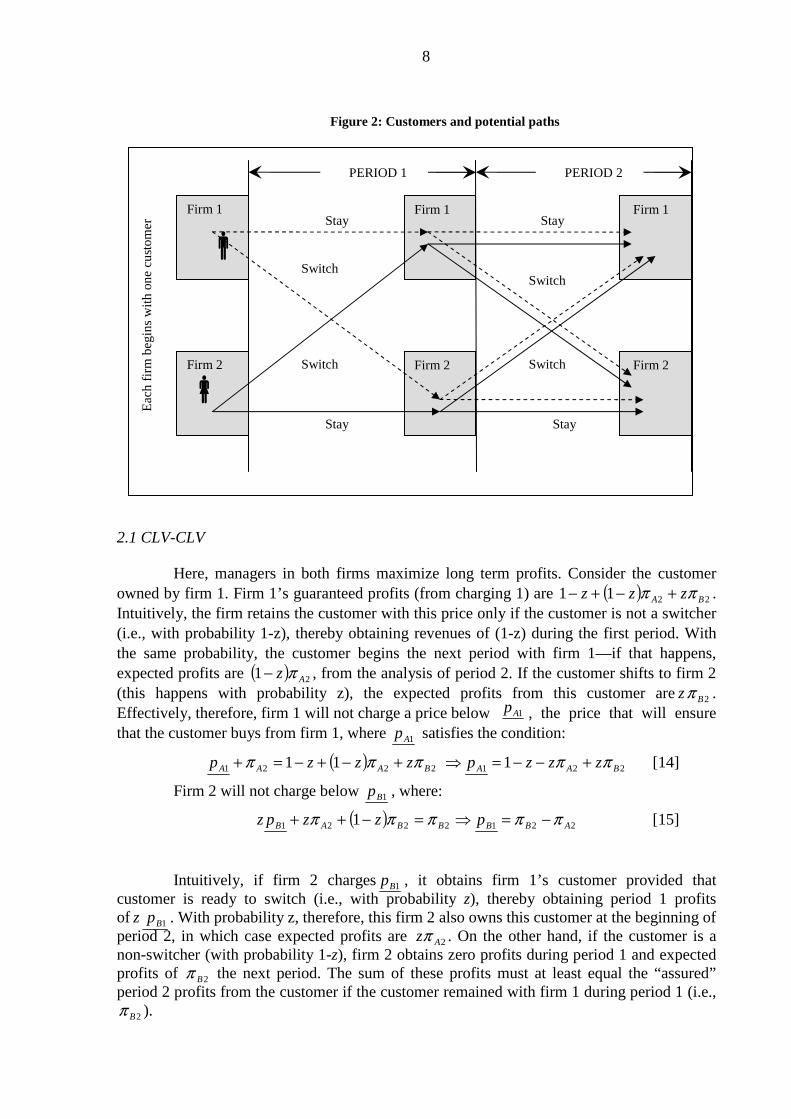
Having established the benchmark case, we extend the game to two periods. Figure 2 provides a graphical description of the two-period game. Effectively, the game described above will constitute the 2nd period of the game—firms make 1st period decisions (with foresight) that can influence whether or not the customer repeat-purchases in period 2 from the same firm. In terms of notation, we append an additional subscript that denotes time; t=1,2. Accordingly, firm 1’s period 2 profits from the customer that it may own at the beginning of that period, and firm 2’s period 2 profits from the same customer are denoted by, respectively (adjusting notation in eqs. 8 and 5):

zA −= 12π ; ( )γπ −−= zzB 12 [12]

Correspondingly, if each firm owns a customer at the beginning of period 2, the total firm profits for period 2 are (adjusting notation in eq. 11):

( )γππππ +−=+== zzBA 1222212 [13]

where ijπ denotes the total profits of firm i in period j.

Let us now consider the first period. Here, firms first decide whether to compensate or rotate managers so that they maximize either period-by-period profits (the ST strategy) or total two-period profits (the CLV strategy). We assume that each firm begins period 1 “owning” a customer. The symmetric cases where both firms focus on either the long term or the short term are of particular interest. These cases represent scenarios where common external pressures or consistent internal cultures lock the firms into a common strategy.

2

1 γ−=z

8

Figure 2: Customers and potential paths

2.1 CLV-CLV

Here, managers in both firms maximize long term profits. Consider the customer owned by firm 1. Firm 1’s guaranteed profits (from charging 1) are ( ) 2211 BA zzz ππ +−+− . Intuitively, the firm retains the customer with this price only if the customer is not a switcher (i.e., with probability 1-z), thereby obtaining revenues of (1-z) during the first period. With the same probability, the customer begins the next period with firm 1—if that happens, expected profits are ( ) 21 Az π− , from the analysis of period 2. If the customer shifts to firm 2 (this happens with probability z), the expected profits from this customer are 2Bzπ . Effectively, therefore, firm 1 will not charge a price below , the price that will ensure that the customer buys from firm 1, where 1Ap satisfies the condition:

( ) 2212221 111 BAABAAA zzzpzzzp πππππ +−−=⇒+−+−=+ [14]

Firm 2 will not charge below 1Bp , where:

( ) 2212221 1 ABBBBAB pzzpz πππππ −=⇒=−++ [15]

Intuitively, if firm 2 charges 1Bp , it obtains firm 1’s customer provided that customer is ready to switch (i.e., with probability z), thereby obtaining period 1 profits of 1Bpz . With probability z, therefore, this firm 2 also owns this customer at the beginning of period 2, in which case expected profits are 2Azπ . On the other hand, if the customer is a non-switcher (with probability 1-z), firm 2 obtains zero profits during period 1 and expected profits of 2Bπ the next period. The sum of these profits must at least equal the “assured” period 2 profits from the customer if the customer remained with firm 1 during period 1 (i.e.,

2Bπ ).

Firm 1

Firm 2

Firm 1

Firm 2

Firm 1

Firm 2

Eac

h fi

rm b

egin

s w

ith

one

cust

omer

PERIOD 1 PERIOD 2

Stay

Stay Stay

Stay

Switch

Switch

Switch

Switch

1Ap

9

In the region 01 >−− γz (which ensures a positive probability of switching in period 2), 11 BA pp >− γ . Following the same reasoning as in § 3.1, a mixed-strategy equilibrium exists in period 1. In this equilibrium, firm 1’s price support is on ]1,( 1Ap and firm 2’s price support is on )1,( 1 γγ −−Ap . Let ( ) ( )pppH AA ≥= 11 Pr and

( ) ( )pppH BB ≥= 11 Pr . In equilibrium, the total profits of firm 1 from the customer it owns at the outset of the game are:

[16]

Here, the terms that are double underlined represent period 2 profits, and the residual terms represent period 1 profits. Likewise the total profits of firm 2 from the customer who is owned by firm 1 at the outset of period 1 are:

[17]

When strategies are mixed, firm 2’s choice of the distribution of prices should be such that firm 1 is indifferent between choosing its upper bound price (of 1) or any other price in the support of its own price distribution. Let us evaluate firm 1’s profits at 1Ap =1:

32221 )2(32)1(1)1( zzzzzzp BAAAA −−+−=+−+−=== γππππ [18]

The lower bound of the support for the price of firm 1, 1Ap , can also be derived. Because a firm should be indifferent between all prices in its price support, on substituting this lower bound price in eq. [16], we should obtain the same profits as in eq. [18]. Using this equality and the facts that ( ) ( ) 1and01 111 =−=− γγ ABB pHH , we obtain:

32221 )2(32)1(1)1( zzzzzzp BAAAA −−+−=+−+−=== γππππ [19]

Substituting for 1Ap and 2Bπ from eq. (12) and solving for 1Ap , we obtain:

γππ 2321 2211 zzzzzzzp BAA −−+−=+−−= [20]

Note that eq. [20] is identical to eq. [14]. The lowest price that firm 2 would charge to the customer of firm 1 is γ−= 11 AB pp . Any price below this would depress profits without increasing the probability of getting the customer to switch. Substituting this price in eq. [17], the profits of firm 2 from this customer are:

[21]

Now, each firm owns a customer at the beginning of period 1. Therefore, the total profits of each firm are the sum of profits from its own customer and that of its competitor:

43221 )2(3)1(2 zzzzBA

CLVCLVCLVCLV −−+−−=+== −− γγππππ [22]

We next analyze the case where managers maximize short term profits.

( ) ( ) ( )[ ]

( ) ( ) ( ) ( ) ( )[ ] 21121121111

21121121

111

11

BABAABAAABA

BABAABAAA

pHzpzHzppHzpz

pHzpHzz

πγπγπγ

πγπγπππ

−−+−+−+−+−=

−−+−+−+=

( ) ( ) ( )[ ]

( ) ( ) ( )[ ] 2112112111

21121121

11)(

11

BBAABABBBA

BBAABABBB

pHzpHzzppHz

pHzpHzz

πγπγπγ

πγπγπππ

+−+++−++=

+−+++−+=

( ) ( ) ( )[ ]( ) ]2)5()3(3[1

11)(23

221

2112112111

γγγππ

πγπγπγπ

−−−−+−=+−+=

+−+++−++=

zzzzzzpz

pHzpHzzppHz

ABB

BBAABABBBAB

10

2.2 ST-ST

The managers in the first period now act as if the game ends during that period itself. Therefore, the period 1 outcome is identical to that obtained in the benchmark case. However, the strategies employed during period 1 influence switching behavior during that period, and hence the opening scenario for period 2.

Let ( ) ( )pppH AA ≥= 11 Pr and ( ) ( )pppH BB ≥= 11 Pr , where, following established notation, 1Ap and 1Bp are period 1 prices charged by firms 1 and 2, respectively, to the customer of firm 1. From the benchmark case (compare with eqs. 4 and 7), we have:

and [23]

Further, profits for each period under ST-ST are identical to eq. [11]. However, period 2 profits have to be adjusted by the appropriate probability that the customers remain with the firms. Now, the probability the customer who begins with firm 1 at the outset of period 1 remains with the firm at the outset of period 2 depends on both the probability that the customer is a non-switcher, and the probability that if the customer is a switcher, the price differential between the firms is sufficiently low that the customer does not switch. Correspondingly, this probability is:

[24]

Likewise, the probability that this customer does switch to firm 2 is denoted by:

[25]

We have adjusted for firm 1’s probability mass point here (see eq. 9). When the customer does switch, this customer begins period 2 with firm 2, and correspondingly, firm 1 obtains expected profits of 2Bπ from that customer in period 2. Therefore, firm 1’s total profits from the customer it owns at the outset of period 1 are:

[26]

Here, from eqs. [5] and [8], zA −= 12π and ( )γπ −−= zzB 12 .

Next consider the customer who is with firm 2 at the outset of period 1. Firm 1’s expected profits from this customer during period 1 are .1Bπ The probability that this customer remains with firm 2 at the outset of period 2 depends both on the probability that the customer is a non-switcher, and the probability that, if the customer is a potential

( )1

11

1

BBA p

zpH

γγ −−=+ ( ) ⎟⎟⎠

⎞⎜⎜⎝

⎛−−=− 1

11

111

AAB pz

zpH γ

∫− ∂

∂−−+−=

1

1

11

1111 )()1(

z

AA

AAB dp

p

HpHzz γψ

⎟⎟⎠

⎞⎜⎜⎝

⎛⎥⎦

⎤⎢⎣

⎡−−−−−−−+⎟⎟

⎠

⎞⎜⎜⎝

⎛ −=γγγγγ

γ z

zzz

z

1

)1)(1(Log)1()(

12

∫− −

−−+∂∂−

−−=1

1

11

1112 1

1)](1[

z

AA

AAB

zzdp

p

HpHz

γγγψ

⎟⎟⎠

⎞⎜⎜⎝

⎛−⎥

⎦

⎤⎢⎣

⎡−−−−−⎟⎟

⎠

⎞⎜⎜⎝

⎛ −−= γγγ

γγ

zz

zz

z

1

)1)(1(Log)1(

12

22211 BAASTST

A πψπψππ ++=−

11

switcher, price differentials are sufficiently low that the customer does not switch. Correspondingly, this probability is:

[27]

Likewise, the probability that this customer does switch to firm 1 is denoted by:

[28]

Note that while we have arrived at these switching probabilities via different routes, reassuringly we have that 11 µψ = and 22 µψ = . This is to be expected with symmetric firms. The total profits that accrue to firm 1 from the customer owned by firm 2 at the outset of period 1 are:

22211 ABBSTST

B πµπµππ ++=− [29]

Now, firms 1 and 2 each own a customer at the beginning of period 1. Therefore, the total profits of each firm are the sum of profits from its own customer and that of its competitor:

== −− STSTSTST21 ππ 22211 BAA

STSTB

STSTA πψπψπππ ++=+ −− + 22211 ABB πµπµπ ++

= 112121 )1()1( BA πµψπµψ +++++ = ))(1(2 γ+− zz [30]

2.3 Comparison of CLV-CLV and ST-ST cases

As noted earlier, CLV-CLV corresponds to the regime where managers in charge of customers over multiple periods seek to maximize the net present value of the customers. In contrast, ST-ST corresponds to the regime where, because of external pressures or for other reasons, managers (who are possibly rotated between periods) maximize short term profits from customers. While a long term focus on customers has been frequently championed, does such an approach yield higher profits? In fact, it does not. Consider the following proposition, which constitutes the key result of the paper:

Proposition 1: Total firm profits under the short term regime (ST-ST) are always (weakly) greater than those under the long term regime (CLV-CLV).

Proof: We need to demonstrate that ≥= −− STSTSTST21 ππ CLVCLVCLVCLV −− = 21 ππ . From

eqs. [22] and [30], this reduces to showing that:

))(1(2 γ+− zz ≥ 432 )2(3)1(2 zzzz −−+−− γγ [31]

On simplifying, this reduces to showing that 0))2(1(2 ≥++−+ γzzz , i.e., 0)2(1 ≥++−+ γzz , i.e.:

[32]

( ) ( )[ ]

⎟⎟⎠

⎞⎜⎜⎝

⎛⎥⎦

⎤⎢⎣

⎡−−−−−−−+⎟⎟

⎠

⎞⎜⎜⎝

⎛ −=

∂∂−+−+−= ∫

−

−−

γγγγγ

γ

γµγ

γ

z

zzz

z

dpp

HpHzz

z

BB

BBA

1

)1)(1(Log)1()(

1

11

2

1

1

11

1111

( )[ ]∫−

−− ∂∂−+=

γ

γ

γµ1

1

11

1112

z

BB

BBA dp

p

HpHz

⎟⎟⎠

⎞⎜⎜⎝

⎛−⎥

⎦

⎤⎢⎣

⎡−−

−−−⎟⎟⎠

⎞⎜⎜⎝

⎛ −−= γγ

γγ

γz

z

zz

z

1

)1)(1(Log)1(

12

z

z 2)1( −−≥γ

12

Now, the probability that the customer is a potential switcher, z, is always (weakly) positive, as is the switching cost γ . Therefore, inequality [32] always holds.

To obtain the intuition, note that the expected profits to each firm during period 1 from its own customer under CLV-CLV are lower than those under ST-ST. These lower profits can be interpreted in terms of investments in the customers, or, alternatively as a “sweetener” that increases the likelihood that the customer stays with the firm. Managers operating in the CLV-CLV regime are open to such bribing because of the shadow of the future—they are pressured not to lose the customers during period 2. In fact, the notion of such investments in customers has frequently been supported in the popular press. The critical point that we highlight is that, in competitive environments, it is very likely that “overinvesting” occurs. Stated differently, when managers are focused on the future in a competitive environment, they are unable to hold back from giving customers a sweet deal that promotes loyalty—however, the resulting loyalty comes at a high cost. Firms are actually better off when, either by rotating managers between periods or otherwise, they force managers to maximize short term profits.

The result established in Proposition 1 is rather general. For the entire parameter space corresponding to 1≤+ γz , we have demonstrated that profits under ST-ST are higher.

Equilibria in short and long term strategies

To demarcate the competitive equilibrium where firms can choose between CLV and ST strategies, we need to analyze the asymmetric CLV-ST and ST-CLV cases, where firms adopt different strategies. The profits to the firms under the possible strategy pairings are captured by a standard payoff matrix, as shown below.

Firm 2: Strategy CLV Firm 2: Strategy ST

Firm 1: Strategy CLV ( )CLVCLVCLVCLV −− ππ , ( )CLVSTSTCLV −− ππ ,

Firm 1: Strategy ST ( )STCLVCLVST −− ππ , ( )STSTSTST −− ππ ,

To consider the equilibrium strategies, we need to solve the two asymmetric scenarios, CLV-ST and ST-CLV, where the firms adopt different strategies. Note that since the focus of analysis is the profits from the customer who is associated with each firm at the outset of period 1, the ST-CLV case is not the mirror image of the CLV-ST case. Specifically, the total profits of each firm are the sum of the (expected) profits from the customer it owns at the outset of period 1, and the (expected) profits from the customer owned by the competitor. Since each firm adopts a different strategy towards these customers, we need to also solve the ST-CLV case separately.

The condition that ensures positive probability of switching in period 2, as explained earlier, is 01 >−− γz . Given this period 2 condition, the following three conditions that govern the nature of the equilibrium in period 1 can be derived:

Condition 1: Under CLV-ST, if , a pure strategy equilibrium exists in period 1 with respect to the customer of firm 1 (the firm that adopts CLV), i.e., there is no switching by this customer in period 1.

)1(1

)1)(1(2

2

zz

zzz −≤≤+

+−− γ

13

Proof: See Appendix A

Condition 2: Under CLV-ST, if , a mixed strategy equilibrium

exists in period 1 with respect to the customer of firm 1 (the firm that adopts CLV), i.e., there

is potentially some switching by this customer in period 1.

Proof: See Appendix A

Condition 3: Under CLV-ST, a mixed strategy equilibrium always exists in period 1 with

respect to the customer of firm 2 (the firm that adopts ST), i.e., there is always potentially

some switching by this customer in period 1.

Proof: See Appendix A

Given these conditions, the profits corresponding to each firm under CLV-ST can be derived.

1 Total firm profits

The profits of each firm under the CLV-ST and ST-CLV outcomes are described below.

Result 1: When Condition 1 holds, the total profits of firm 1 (CLV) and firm 2 (ST) are:

STCLV −Π = ]3)1(1)[1( 2zzzz −+−+− γ [33]

CLVST −Π = [34]

Proof: See Appendix A

Result 2: When Condition 2 holds, the total profits of firm 1 (CLV) and firm 2 (ST) are:

=Π −STCLV )](1[2 γ+− zz [35]

CLVST −Π 2)1()1( Azz π−+−=

2

2

1

)1)(1(0

z

zzz

++−−<≤ γ

⎥⎥⎥

⎦

⎤

⎢⎢⎢

⎣

⎡

⎥⎦

⎤⎢⎣

⎡−−−−−+

−−−−++++−−−

−−)-z-(2z--2

-z-2Log)]2(1)[2(

)]1()1)(221()2()3()[1(

)1(

1332222

2

γγγγγ

γγγγ

γ zzz

zzzzzzz

z

14

[ ] 2111

11

1

211211 )1()(

)](1[)( BCLVST

AAA

CLVSTA

z

BACLVST

BAACLVST

B Hzdpp

pHpHpHz ππγπγ −

−

−

−− +⎟⎟⎠

⎞⎜⎜⎝

⎛

∂∂−

−−+−+ ∫

2

1

11

111

2

1

11

1111

1

1

)](

)](1[)1(

A

p

BB

STCLVB

BSTCLV

A

B

p

BB

STCLVB

BSTCLV

AB

A

A

dpp

HpHz

dpp

HpHzz

πγ

πγπ

γ

γ

γ

γ

⎥⎥⎦

⎤

⎢⎢⎣

⎡

∂∂−++

⎥⎥⎦

⎤

⎢⎢⎣

⎡

∂∂−

+−+−++

∫

∫

−

−

−−

−

−

−−

[36]

where ( )γππ −−=−= zzz BA 1;1 22

( )γπππ −+−−= 221 1 BAB zzzz ; 321 )2(21 zzzpA −−+−= γ

( )

( ) ;111

;1

1

22

221

⎟⎟⎠

⎞⎜⎜⎝

⎛−

+−=

−+−−+−−=

−

−

γ

ππγππγ

pz

zpH

p

zpH

CLVSTB

BA

BACLVSTA

( )

( ) ;111

;1

1

22

221

⎟⎟⎠

⎞⎜⎜⎝

⎛−

+−=

−+−−+−−=

−

−

γ

ππγππγ

pz

zpH

p

zpH

CLVSTB

BA

BACLVSTA

(While these profits can be evaluated in closed form as a function of z and γ , the resulting expression is complex and is not reproduced here.)

Proof: See Appendix A

2. Profit comparisons and derivation of equilibria

As seen in Figure 3, the parameter space defined by 1≤+ γz can be divided into two parts, corresponding to Conditions 1 and 2. We consider the equilibria in each region separately.

Condition 1: )1(1

)1)(1(2

2

zz

zzz −≤≤+

+−− γ

First, consider CLV-ST. Through simple algebraic manipulations, it can be

demonstrated that:

STCLV −Π (from eq. 33) ≥ STST −Π (from eq. 30) )1(1

)1)(1(2

2

zz

zzz −≤≤+

+−−∀ γ [37]

Therefore, ST-ST is not a Nash equilibrium in Condition 1, since one firm will unilaterally shift from ST to CLV. Next, consider CLV-CLV. It can be numerically demonstrated that:

CLVCLV −Π (from eq. 22) ≥ CLVST −Π (from eq. 34) )1(1

)1)(1(2

2

zz

zzz −≤≤+

+−−∀ γ [38]

15

Therefore, CLV-CLV is a Nash equilibrium in Condition 1, since no firm will unilaterally shift from CLV to ST. The inequality in eq. [38] also implies that the firm that implements ST under ST-CLV has the incentive to unilaterally shift from ST to CLV—therefore, the asymmetric strategy pairing does not constitute a Nash equilibrium. Summarizing these results:

PROPOSITION 2: Under Condition 1, i.e., when , the symmetric case where both firms engage in customer lifetime value maximization, i.e., CLV-CLV, constitutes the sole Nash equilibrium. While ST-ST does not constitute a Nash equilibrium, firm profits under ST-ST are always (weakly) higher than under CLV-CLV.

Condition 2: 2

2

1

)1)(1(0

z

zzz

++−−≤≤ γ

First, consider ST-ST. Comparing eqs. [30] and [35], STST −Π = STCLV −Π . Therefore, no firm has the (strong) incentive to unilaterally shift to CLV from ST, and ST-ST constitutes a Nash equilibrium in Condition 2. Next, consider CLV-CLV. It can be numerically demonstrated that:

CLVCLV −Π (from eq. 22) ≥

CLVST −Π(from eq. 36)

2

2

1

)1)(1(0

z

zzz

++−−≤≤∀ γ

[39]

Therefore, no firm has the incentive to unilaterally shift to ST from CLV, and CLV-CLV constitutes a Nash equilibrium in Condition 2. Further, the inequality in eq. (39) implies that the asymmetric strategy pairing does not constitute a Nash equilibrium. Summarizing these results:

PROPOSITION 3: Under Condition 2, i.e., when , both ST-ST and CLV-CLV constitute Nash equilibria. However, given that STST −Π ≥ CLVCLV −Π CLVST −Π (see Proposition 1), ST-ST constitutes the Pareto-dominant equilibrium.

Equilibrium regions are graphically demarcated in Figure 3.

)1(1

)1)(1(2

2

zz

zzz −≤≤+

+−− γ

2

2

1

)1)(1(0

z

zzz

++−−≤≤ γ

16

Figure 3: Equilibria in strategies

3 Discussion

The results indicate that for the entire relevant parametric region (i.e., 1≤+ γz ), firms attain the highest profit when their managers are engaged in short term profit maximization. As discussed earlier, firms may indeed be locked into such a strategy on account of pressures from the environment, particularly from the financial market. Correspondingly, firms must carefully consider the advantages and disadvantages of disturbing this status quo before they encourage their managers to focus on the long term with respect to their customers.

When firms are not locked into short term profit maximization and can instead choose between short term and long term (CLV) maximization, the equilibrium in incentive plans is a function of the specific combination of parameters z andγ . Specifically, when z and/or γ are relatively high (the relatively small region corresponding to Condition 1 in Figure 3), the sole equilibrium involves the maximization of CLV by both firms, though profits under a symmetric short term focus (i.e., ST-ST) are higher for both firms. Under all other parameter combinations (i.e., Condition 2 in Figure 3), both CLV-CLV and ST-ST constitute equilibria. However, the ST-ST equilibrium is Pareto-dominant since each firm obtains higher profits here.

Overall, our results suggest that, in competitive environments, firms likely erode total profits when they adopt a long term approach in seeking to maximize the lifetime value of their customers. While this prescription would correctly apply to a monopolist, the implications of adopting such a strategy for the competitive equilibrium must first be carefully thought through in markets where firms compete for customers. Paradoxically, customer lifetime value may be maximized when managers focus on the short term, rather than the long term.

γ (Switching cost)

Condition 1: CLV-CLV is the sole Nash equilibrium

Condition 2: Both CLV-CLV and ST-ST are

Nash equilibria. ST-ST is the pareto-

dominant equilibrium

z (P

roba

bili

ty o

f bei

ng

a po

tent

ial s

witc

her)

0,0 1

1

2

2

1

)1)(1(

z

zzz

++−−=γ

z−=1γ

17

Two extensions

Proponents of customer lifetime value maximization have argued that such an approach can result in (a) enhanced revenues from long-term customers, and (b) lower costs of serving them. Since our existing analysis does not account for these effects, one may question whether our findings are robust. To address this issue, we extend the basic model in two directions. First, we allow for a “revenue expansion effect” that may occur, for example, when the firm gains deeper knowledge of loyal customers over time. Second, we allow for a “cost reduction effect” that may occur when the firm learns to efficiently serve loyal customers. To examine these effects, we first assume that the marginal cost of firm’s offering is c>0. The effects are operationalized as follows:

(a) Revenue expansion effect: Consider a customer who begins with firm i at the outset of period 1 and purchases from firm i in period 1. If this customer purchases from firm i in period 2, the purchased quantity is (1+δ ) rather than 1, i.e., firm i gains a larger share of wallet.

(b) Cost reduction effect: Consider a customer who begins with firm i at the outset of period 1 and purchases from firm i in period 1. If this customer purchases from firm i in period 2, the cost of providing the product or service to the customer is )1( δ−=′ cc , ).1,0(∈δ

In each case, a higher value of δ indicates a stronger effect. We compare the implications of these effects across the two symmetric regimes, i.e., ST-ST, and CLV-CLV, for two reasons. First, the asymmetric cases do not emerge as equilibria in the baseline model without these effects (see Figure 3). Second, this substantially reduces analytical complexity8.

The profit expressions corresponding to the CLV-CLV and ST-ST outcomes can be analytically derived (see eqs. a64, a76, and a77 in the Appendix). The complexity of these closed form expressions precludes an analytical comparison of profits across cases. In Table 1 below, we numerically confirm that the profits under ST-ST are greater than under CLV-CLV.

The first two cases in Table 1 correspond to z = 0, i.e., there is no switching. Each firm exercises monopoly power over the customer it owns. As seen in Case 1, when there is no switching and, in addition, δ = 0 (i.e., there is no cost reduction or revenue expansion at work), profits across all strategy pairings are identical, i.e., whether the firm engages in CLV or ST is irrelevant. As seen in Case 2, profits are higher when δ > 0 (compared to Case 1 where δ = 0).

In Case 3, there is a positive, but relatively low probability of switching (i.e., z = 0.25). Across the board, profits decrease compared to Case 2—however, note that (a) under both ST-ST and CLV-CLV, profits are (weakly) higher when δ = 0.25 (compared to δ = 0), and (b) profits under ST-ST are consistently higher than those under CLV-CLV. Similarly, comparing Case 3 to Cases 4 and 5, while profits decrease across the board as z increases (from 0.25 to 0.35 and 0.50, respectively), profits under ST-ST are consistently higher than under CLV-CLV.

Comparing Case 3 to Cases 6 and 7 reveals the implications of a higher switching costγ . Profits decrease across the board as γ increases (from 0.25 to 0.35 and 0.50, respectively). Again, profits under ST-ST are higher than those under CLV-CLV across the cases.

8 The analysis for the asymmetric cases is available from the authors on request. As before, the asymmetric outcomes do not constitute Nash equilibria, even when a revenue expansion or a cost reduction effect applies.

18

Comparing Case 3 to Cases 8 and 9 reveals the implications of a higher revenue expansion (or, alternatively, cost reduction parameter) δ. Profits increase across the board as δ increases (from 0.25 to 0.35 and 0.50, respectively). Again, profits under ST-ST are consistently higher than under CLV-CLV across these cases.

The most interesting finding so far is that a short term focus yields higher profits than a long term focus even when keeping customers over the long run pays off in terms of either a higher share-of-wallet or a lower cost to serve. Intuitively, each of these loyalty-driven effects enhances the value of the proverbial pot of gold at the end of the rainbow. However, such potential rewards accentuate the competition to gain and keep customers—the larger the pot, the more intense the short-term competition. Consistent with this reasoning, ignoring the potential to enhance the pot during the early stages of the game (as under ST-ST) leads to higher overall profits.

Cases 10 and 11 represent highly competitive scenarios with high customer switching probabilities (z) and low switching costs (γ ). As expected, profits across strategy pairings drop compared to the corresponding pairings within Cases 1-9. However, what is striking in Cases 10 and 11 is that profits under CLV-CLV and ST-ST when δ = 0 (i.e., in the absence of revenue enhancement and cost reduction effects) are weakly higher than the corresponding profits in the presence of revenue enhancement and cost reduction effects. Further, comparing Cases 10 and 11, profits decrease as the magnitude of these effects increase.

The intuition here is that, when the market is already highly competitive, enhancing the value of the pot at the end of the rainbow can increase short run price competition to such an extent that, irrespective of whether a short term (ST) or a long term (CLV) strategy is adopted, overall profits decrease. Further, comparing across Cases 10 and 11, as the strength of the revenue enhancement or cost reduction effect increases, profits decrease further. Apart from these effects, though, profits under ST-ST are consistently higher than under CLV-CLV in Cases 10 and 11 as well. These findings attest to the robustness of our central argument that customer lifetime value is maximized in competitive environments when managers focus on the short term.9

.

9 A grid search of the parametric space revealed no values that contradict the key findings in Table 1.

19

Table 1.: Profits under CLV-CLV and ST-ST strategy pairings

Cases Parameter values CLV-CLV

(δ = 0)

ST-ST

(δ = 0) δ

CLV-CLV (with

revenue expansion)

ST-ST

(with revenue

expansion)

CLV-CLV (with cost reduction)

ST-ST

(with cost reduction)

1. c = 0.25; z = 0; γ = 0.25 1.5 1.5 0.00 1.5 1.5 1.5 1.5

2. c = 0.25; z = 0; γ = 0.25 1.5 1.5 0.25 1.69 1.69 1.56 1.56

3. c = 0.25; z = 0.25; γ = 0.25 1.25 1.28 0.25 1.34 1.39 1.28 1.32

4. c = 0.25; z = 0.35; γ = 0.25 1.09 1.14 0.25 1.14 1.22 1.11 1.17

5. c = 0.25; z = 0.50; γ = 0.25 0.80 0.86 0.25 0.80 0.91 0.80 0.89

6. c = 0.25; z = 0.25; γ = 0.35 1.20 1.23 0.25 1.29 1.34 1.23 1.27

7. c = 0.25; z = 0.25; γ = 0.50 1.12 1.16 0.25 1.21 1.27 1.15 1.19

8. c = 0.25; z = 0.25; γ = 0.25 1.25 1.28 0.35 1.37 1.43 1.30 1.33

9. c = 0.25; z = 0.25; γ = 0.25 1.25 1.28 0.50 1.43 1.49 1.31 1.35

10. c = 0.25; z = 0.75; γ = 0.01 0.61 0.64 0.10 0.59 0.63 0.61 0.64

11. c = 0.25; z = 0.75; γ = 0.01 0.61 0.64 0.25 0.57 0.61 0.60 0.63

20

Conclusion

Researchers and practitioners have advanced the view that, towards maximizing customer lifetime value, managers must adopt a long term horizon while managing customer relationships. However, this view may not have sufficiently accommodated the competitive implications of a long term approach. Our results suggest that customer lifetime value may be maximized in competitive environments when managers instead focus on the short term.

A two-period model of a duopoly in which each firm began with one customer was first introduced. Each customer could be a potential switcher with a certain probability, and would incur a certain switching cost if the customer who was a potential switcher indeed switched firms. Using this simple setup, total firm profits under a short-term focus where the managers in each firm maximized period-by-period profits were shown to be always higher than when they maximized long term profits from the customers. Further, it was demonstrated that the asymmetric cases where managers in one firm focused on per-period profits and managers in the other focused on total two-period profits did not constitute Nash equilibria.

Next, to accommodate some of the frequently highlighted benefits of retaining customers, each firm was allowed to either garner enhanced revenues from, or lower its costs to serve, customers who remained with the firm over multiple periods. However, the incorporation of such revenue enhancement and cost reduction effects did not alter the superiority of the short-term focus over the long-term focus. Finally, it was demonstrated that when competition is intense (corresponding to the case where the probability that customers were potential switchers was high and switching costs were low), a stronger revenue enhancement or cost reduction effect could, in fact, lower total profits, irrespective of whether managers focus on the short term or the long term.

From a managerial perspective, our findings suggest that decisions to reorient business processes, align managerial incentives, and implement CRM technologies to facilitate a long term orientation towards customers deserve careful evaluation, particularly when these decisions are driven by normative pressures to jump aboard the bandwagon. In competitive environments, managers must carefully evaluate the strategic implications of such initiatives both prospectively and on an ongoing basis. Managers must be alert for signs of increase in the intensity of short term competition, and must rigorously evaluate the corresponding implications for the profitability of the customer base. Further, managers must approach the counterintuitive notion that a short term focus may yield superior overall profits with an open mind.

From a research perspective, the competitive implications of short term and long term foci in the context of CRM have received relatively little attention. This paper sheds some new light on how, contrary to popular beliefs, a long term focus can yield lower total profits than a short term focus in competitive environments. At the least, our findings suggest that informal arguments and formal models that support the superiority of a long term focus with respect to customers are incomplete without addressing the corresponding competitive implications.

This paper represents an early effort to examine the competitive implications of short term and long term foci in the context of CRM. As the next step, we aim to examine the competitive implications of a “mixed” focus, where the components of incentive plans are based on both short term and long term profits.

21

References

Beggs, A. and P. Klemperer. 1992. Multi-Period Competition with Switching Costs. Econometrica 60 (3) 651-666.

Blattberg, R. C. and J. Deighton. 1996. Manage Marketing by the Customer Equity Test. Harvard Business Review 74 (4) 136-44.

Blattberg, R. C., G. Getz and J. S. Thomas. 2001. Customer Equity: Building and Managing Relationships as Valuable Assets. Cambridge MA: Harvard Business School Press.

Chen, Y. 1997. Paying Customers to Switch. Journal of Economics and Management Strategy 6 (4) 877-897.

Chen, Y., C. Narasimhan and Z. J. Zhang. 2001. Individual Marketing with Imperfect Targetability. Marketing Science 20 (1) 23-41.

Farrell, J. and C. Shapiro. 1988. Dynamic Competition with Switching Costs. The RAND Journal of Economics. 19 123-137.

Fudenberg, D. and J. Tirole. 2000. Customer Poaching and Brand Switching. The RAND Journal of Economics. 31 634-657.

Klemperer, P. 1987a. The Competitiveness of Markets with Switching Costs. The RAND Journal of Economics. 18 (1) 138-150.

——— 1987b. Markets with Consumer Switching Costs. The Quarterly Journal of Economics. 102 (2) 375-394.

——— 1989. Price Wars Caused by Switching Costs. The Review of Economic Studies. 56 (3) 405-420.

——— 1995. Competition when Consumers have Switching Costs: An Overview with Applications to Industrial Organization, Macroeconomics, and International Trade. The Review of Economic Studies 62 (4) 515-539.

Kopalle, P. K. and S. A. Neslin. 2003. The Economic Viability of Frequency Reward Programs in a Strategic Competitive Environment. Review of Marketing Science. 1 (Available at: www.bepress.com/romsjournal/vol1/iss1/art1).

McGahan, A. M. and P. Ghemawat. 1994. Competition to Retain Customers. Marketing Science 13 (2) 165-76.

Narasimhan, C. 1988. Competitive Promotional Strategies. Journal of Business 61 (4) 427-49.

Padilla, A. J. 1992. Mixed Pricing in Oligopoly with Consumer Switching Costs. International Journal of Industrial Organization 10 393-412.

Reinartz, W. and V. Kumar. 2000. On the Profitability of Long-Life Customers in a Noncontractual Setting: An Empirical Investigation and Implications for Marketing. Journal of Marketing 64 (4) 17-35.

__________ and ________. 2002. The Mismanagement of Customer Loyalty. Harvard Business Review July 86-97.

Rust, R., V. A. Zeithaml and K. Lemon. 2000. Driving Customer Equity: How Customer Lifetime Value is Reshaping Corporate Strategy. New York: Free Press.

22

Shaffer, G. and Z. J. Zhang. 1995. Competitive Coupon Targeting. Marketing Science 14 (4) 395-416.

Shaffer, G. and Z. J. Zhang. 2002. Competitive One-to-One Promotions. Management Science. 48 1143-1160.

Varian, H. R. 1980. A Model of Sales. American Economic Review 70 651-659.

Villas-Boas, J. M. 1999. Dynamic Competition with Customer Recognition. RAND Journal of Economics 30 (4) 604-31.

Winer, R. 2001. A Framework for Customer Relationship Management. California Management Review 43 (4) 89-105.

vonWeizsacker, C. 1984. The Costs of Substitution. Econometrica 52(5) 1085-1116.

23

Appendix A

MANAGING CUSTOMER RELATIONSHIPS: SHOULD MANAGERS REALLY FOCUS ON THE LONG TERM?

A1. Asymmetric Cases

Under CLV-ST, firm 1 adopts CLV, and firm 2 adopts ST. Consider first the customer who belongs to firm 1 at the outset of period 1. If firm 1 prices at 1 during period 1 to its own customer, its (guaranteed) expected profits are (1-z)+(1-z) 2Aπ + z 2Bπ . This reflects the probability that firm 1 will retain the customer in period 2 only if that customer is a non-switcher (i.e., with probability 1-z). Therefore, firm 1 will never price below lower bound

1Ap , such that:

=+ 21 AAp π (1-z)+(1-z) 2Aπ + z 2Bπ , i.e., 321 )2(21 zzzpA −−+−= γ [a1]

The manager in firm 2 maximizes period 1 profits alone, and will not price below cost:

01 =Bp [a2]

Condition 1: Under CLV-ST, if , a pure strategy equilibrium

exists in period 1 with respect to the customer of firm 1 (that adopts CLV), i.e., there is no

switching by this customer in period 1.

Proof:

We know that if 011 =≤− BA pp γ , there is no switching in period 1, and a pure strategy equilibrium exists. From eqs. (a1) and (a2), this occurs when:

2

2

1

)1)(1(

z

zzz

++−−≥γ [a3]

Here, firm 2 charges 01 =Bp , and firm 1 charges γγ =+= 11 BA pp . We know that

the condition for switching in period 2 i s )1( z−≤γ . Also,

because ( )22 1)1( zzz +<+− . Hence, the condition for pure strategy in period 1 is the one

given above.

Condition 2: Under CLV-ST, if a mixed strategy equilibrium

exists in period 1 with respect to the customer of firm 1 (that adopts CLV), i.e., there is

potentially some switching by this customer in period 1.

Proof:

If 011 =>− BA pp γ , there is potentially some switching in period 1, and a mixed strategy equilibrium exists. Substituting prices from eqs. [a1] and [a2], this occurs when:

)1(1

)1)(1(2

2

zz

zzz −≤≤+

+−− γ

( )zz

zzz −<+

+−−1

1

)1)(1(2

2

2

2

1

)1)(1(0

z

zzz

++−−<≤ γ

24

2

2

1

)1)(1(0

z

zzz

++−−<≤ γ

Condition 3: Under CLV-ST, a mixed strategy equilibrium always exists in period 1 with respect to the customer of firm 2 (the firm that adopts ST), i.e., there is always potentially some switching by this customer in period 1.

Proof:

Consider the customer of firm 1 under ST-CLV. In period 1, firm 1 can guarantee itself expected profits of (1-z) from this customer by charging a reservation price of 1—hence, it will not price below .11 zpA −= Firm 2 will not offer a price below 1Bp , which satisfies:

2221 )1( BBAB zzpz πππ =−++ , i.e., 221 ABBp ππ −= [a4]

Now, if 11 BA pp <− γ , there is no switching in period 1 since firm 1 will always retain its customer by pricing sufficiently low. Given that ( )zA −= 12π and ( )γπ −−= zzB 12 , the condition translates to 2>+ γz , which is not feasible given that both z and γ lie in the interval (0,1]. Therefore, only a mixed strategy equilibrium exists in period 1.

Profits under CLV-ST from customer starting with Firm 1

Under Condition 1, a pure strategy equilibrium exists in period 1. Here, firm 2 charges 01 =Bp , and firm 1 charges γγ =+= 11 BA pp . Intuitively, firm 1 is able to price low enough here that it can get the customer for sure. Firm 1’s expected profits from its own customer are:

γπγπ +−=+=− zASTCLV

A 12 [a5]

Firm 2’s expected profits from the customer of firm 1 are:

)1(0 2 γππ −−=+=− zzBSTCLV

B [a6]

Under Condition 2, a mixed strategy equilibrium exists in period 1. Following reasoning similar to that articulated earlier, the price supports of firms 1 and 2 are respectively ]1,( 1Ap and ]1,( 1 γγ −−Ap . As in case 1 (eq. a1), 32

1 )2(21 zzzpA −−+−= γ . Let ( ) ( )pppH AA ≥= 11 Pr and ( ) ( )pppH BB ≥= 11 Pr . In equilibrium, the total profits (across two periods) that accrue to firm 1 from the customer that it owns at the outset of period 1 are:

])](1[)()1[(

)]()1[(

2112112

11121

BABAABA

AABAAA

pHzpHzz

ppHzz

πγπγπγπππ

−−+−+−+−+−=+=

[a7]

Likewise, the profits of firm 2 in period 1 from the customer of firm 1 are:

1111 )( BBAB ppHz γπ += [a8]

Now, 1)(,0)1( 111 =−=− γγ ABB pHH , and 1)( 11 =AA pH . Evaluating eq. (a7) at 11 AA pp = :

25

=+=−21 AA

STCLVA p ππ =−+−−+− )1()2(21 32 zzzz γ 32)2(32 zzz −−+− γ [a9]

Similarly, evaluating eq. (a8) at firm 2’s lower bound price γ−= 11 AB pp , we have:

zppHzppHz AAABBAB =−=+= )()()( 1111111 γγπ ))2(21( 32 γγ −−−+− zzz [a10]

Next, substituting eq. [a10] in eq. [a8]:

)(

)( 11 γ

π−

=pz

pH BA =

γγγ

−−−−+−

p

zzz ))2(21( 32

[a11]

Likewise, substituting eq. (a9) into eq. (a7) and solving for )(1 pH B , we obtain:

)(

)1)(1()(

221

BAB pz

pzpH

ππγγ

−++−−−=

))2(1(

)1)(1(2zzpz

pz

+−−++−−−=γγ

γ [a12]

Therefore, firm 2’s profits from the customer owned by firm 1 at the outset of period 1 are:

[a13]

Note that since the focus of analysis is the customer associated with each firm, to derive the total profits of each firm in the asymmetric case, we need to first solve the ST-CLV case as well.

Profits under ST-CLV from customer starting with Firm 1

According to Condition 3, only a mixed strategy equilibrium exists in period 1, when the price supports of firms 1 and 2 are ]1,( 1Ap and ]1,( 1 γγ −−Ap , respectively. As before, let ( ) ( )pppH AA ≥= 11 Pr and ( ) ( )pppH BB ≥= 11 Pr . If firm 1 charges a price of 1Ap to its customers, its expected period 1 profits from this customer are:

11111 )()1( AABAA ppHzpz γπ −+−= [a14]

Intuitively, firm 1 obtains profits that equal 1Ap if the customer is not a potential switcher—if the customer is a potential switcher, the profits then depend on the probability that firm 2’s price is sufficiently high that the customer decides to stay with firm 1. Firm 2’s total profits from this customer across the two periods equal:

])](1[)()1[()( 2112112111 BBAABABBBAB pHzpHzzppHz πγπγπγπ +−+++−++= [a15]

2

1

11

111

2

1

11

1111

1

1

)](

)](1[)1(

A

p

BB

BBA

B

p

BB

BBAB

STCLVB

A

A

dpp

HpHz

dpp

HpHzz

πγ

πγππ

γ

γ

γ

γ

⎥⎥⎦

⎤

⎢⎢⎣

⎡

∂∂−

++

⎥⎥⎦

⎤

⎢⎢⎣

⎡

∂∂−

+−+−+=

∫

∫

−

−

−

−

−

26

We know that 1)(,0)1( 111 =−=− γγ ABB pHH , and 1)( 11 =AA pH . Evaluating eq. [a14] at 11 =Ap , and using the fact that in a mixed strategy equilibrium firm 2’s mixing probabilities must be such that firm 1 is indifferent between pricing at any point in its price support, we have:

zA −= 11π [a16]

Likewise, evaluating eq. (a15) at the lower bound of firm 2’s price support (i.e., at γ−−= zpB 11 ), firm 2’s total profits from the customer who begins with firm 1 are:

22)1()1( ABCLVST

B zzzz ππγπ +−+−−=− = )]4(23[ γγ −−−− zzz [a17]

Evaluating eq. [a15] at ppB =+ γ1 and equating the resulting expression to eq. [a17], we obtain:

22

221

1)(

BA

BAA p

zpH

ππγππγ

−+−−+−−

= [a18]

Note that the corresponding distribution of firm 1’s prices to its own customer has a mass point at 11 =Ap . Evaluating eq. (a14) at ppA =− γ1 and equating the result to eq. [a16], we obtain:

⎟⎟⎠

⎞⎜⎜⎝

⎛−

+⎟⎠⎞

⎜⎝⎛ −= 1

11)(1 γpz

zpH B [a19]

The total profits of firm 1 from its own customer can now be specified:

[ ] 2111

11

1

211211

221

)1()(

)](1[)(

)1()1(

BAAA

A

z

BABAAB

AAACLVST

A

Hzdpp

pHpHpHz

zz

ππγπγ

ππππ

+⎟⎟⎠

⎞⎜⎜⎝

⎛

∂∂−

−−+−+

−+−=+=

∫−

−

[a20]

Note that while computing profits in eq. [a20] we have adjusted for firm 1’s probability mass point at .11 =Ap Having solved the CLV-ST and ST-CLV cases, we can derive total firm profits.

Total Profits

The profits of the firm that engages in CLV are the sum of the profits from its own customer and that of its competitor (ST). When Condition 1 holds (Result 1), the total profits of firm 1 (CLV) are the sum of eqs. (a5) and (a17):

CLVSTB

STCLV z −− ++−=Π πγ1 ]3)1(1)[1( 2zzzz −+−+− γ = [a21]

The total profits of firm 2 (ST) are the sum of the profits from its own customer and from the customer of its competitor (CLV), i.e., the sum of eqs. [a6] and [a20]:

= [a22]

⎥⎥⎥

⎦

⎤

⎢⎢⎢

⎣

⎡

⎥⎦

⎤⎢⎣

⎡−−−−−+

−−−−++++−−−

−−)-z-(2z--2

-z-2Log)]2(1)[2(

)]1()1)(221()2()3()[1(

)1(

1332222

2

γγγγγ

γγγγ

γ zzz

zzzzzzz

z

CLVSTA

CLVST zz −− +−−=Π πγ )1(

27

When Condition 2 holds (Result 2) the total profits of firm 1 are the sum of eqs. [a9] and [a17]:

CLVSTB

STCLVA

STCLV −−− +=Π ππ = )](1[2 γ+− zz [a23]

The total profits of firm 2 (ST) are the sum of eqs. [a13] and [a20]:

STCLVB

CLVSTA

CLVST −−− +=Π ππ [a24]

CLVST −Π 2)1()1( Azz π−+−=

[a25]

where: ( )γππ −−=−= zzz BA 1;1 22 ;

( )γπππ −+−−= 221 1 BAB zzzz ; 321 )2(21 zzzpA −−+−= γ

( )

( ) ;111

;1

1

22

221

⎟⎟⎠

⎞⎜⎜⎝

⎛−

+−=

−+−−+−−=

−

−

γ

ππγππγ

pz

zpH

p

zpH

CLVSTB

BA

BACLVSTA

⎥⎦

⎤⎢⎣

⎡−

+−++−−=

−−+−−

=

−

−

111

1

22

221

221

γππππ

γγππ

BA

BASTCLVB

BASTCLVA

pz

zH

p

zzzH

[ ] 2111

11

1

211211 )1()(

)](1[)( BCLVST

AAA

CLVSTA

z

BACLVST

BAACLVST

B Hzdpp

pHpHpHz ππγπγ −

−

−

−− +⎟⎟⎠

⎞⎜⎜⎝

⎛

∂∂−−−+−+ ∫

2

1

11

111

2

1

11

1111

1

1

)](

)](1[)1(

A

p

BB

STCLVB

BSTCLV

A

B

p

BB

STCLVB

BSTCLV

AB

A

A

dpp

HpHz

dpp

HpHzz

πγ

πγπ

γ

γ

γ

γ

⎥⎥⎦

⎤

⎢⎢⎣

⎡

∂∂−

++

⎥⎥⎦

⎤

⎢⎢⎣

⎡

∂∂−

+−+−++

∫

∫

−

−

−−

−

−

−−

28

Appendix B

MANAGING CUSTOMER RELATIONSHIPS: SHOULD MANAGERS REALLY FOCUS ON THE LONG TERM?

To incorporate the revenue expansion and cost reduction effects, we first solve a model with a positive marginal cost.

B1. Period 2 model with a positive marginal cost c

We first solve the benchmark case (one period model) with a positive marginal cost c but without the application of a revenue enhancement or cost reduction effect. As before, each firm begins the period with a customer. Denote firm 1’s profit from its customer as Aπ and firm 2’s profit from the same customer as Bπ . Let prices offered to this customer from these two firms be Ap and Bp , respectively. Now, if firm 1 charges a price of 1, it is guaranteed a profit of (1-z)(1-c), which is the probability that the customer is a non-switcher. Therefore, to avoid receiving less than these guaranteed profits, firm 1 will not set a price below Ap , such that )1)(1( czcpA −−=− , i.e., cczpA +−−= )1)(1( . Firm 2 will not charge below cost c.

We assume that there is always a positive likelihood of customer “churn” in equilibrium—this corresponds to the case where Ap γ>− Bp . Following the same reasoning as in § 3.1, no pair of prices can constitute a pure-strategy equilibrium in this region—however, a mixed strategy equilibrium exists. In this equilibrium, firm 1’s price support is

]1,( Ap (see above) and firm 2’s price support is ]1,( γγ −−Ap . Let ( ) ( )pppH AA ≥= Pr and ( ) ( )pppH BB ≥= Pr . The equilibrium profits of firms 1 and 2 from the customer of firm 1 are:

))](()1[( cppHzz AABA −−+−= γπ [a26]

)()( cppHz BBAB −+= γπ [a27]

We also know that ( ) ( ) ( ) 1 and,1,01 ==−=− AAABB pHpHH γγ . Now, firm 1 chooses the mixing strategy (.)AH such that firm 2 is indifferent between choosing the lower bound price of γ−Ap , in which case it conquers the customer with probability z (i.e., if the customer is in a switching mode), or any other price. Therefore:

))(()( cppHzcpz BBAA −+=−− γγ , i.e., ( ))(

)1)(1(

cp

czpH

BBA −

−−−=+ γγ , i.e.,

( ))(

)1)(1(

cp

czpH A −−

−−−=γ

γ

[a28]

Substituting the expression for ( )γ+BA pH from [a28] in [a27],

])1)(1[( γπ −−−= czzB [a29]

Similarly, firm 2 chooses the mixing strategy (.)BH such that firm 1 is indifferent between choosing the upper bound price of 1 and obtaining a expected profit of (1-z)(1-c), corresponding to the probability that the customer is a switcher, or any other price. Therefore:

29

( ) ( )γ−−+−−=−− ABAA pHcpzzcpcz )(1)()1)(1( , i.e., ( ) ⎟⎟⎠

⎞⎜⎜⎝

⎛−+−−−=

cp

p

z

zpH B γ

γ1)1( [a30]

Substituting (a30) into (a26), the profits of firm 1 are:

)1)(1( czA −−=π [a31]

B2. Period 2 model with positive marginal cost and revenue expansion effect

This corresponds to the case where the customer begins with one firm at the outset of period 1, and purchases from the same firm during period 1.

When the customer who begins with a firm at the outset of period 1 stays with the same firm during period 1, then the customer with a reservation price of 1 per unit purchases (1+δ ) units from that firm during period 2, conditional on the customer staying with the firm during period 2. If that customer switches firms during period 2, the customer purchases 1 unit.

Without loss of generality, we focus on a customer who begins with firm 1 at the outset of period 1 and purchases from that firm during period 1. If this customer were to purchase from firm 1 during period 2 as well, the purchase quantity is (1+δ ). If the customer is a potential switcher (i.e., with probability z), this customer shifts to firm 2 during period 2 if the surplus gained from switching is positive, i.e., if:

γδ >+−−− )1)(1(1)1( AB pp , i.e., γδ −+−−< )1)(1(1 AB pp [a32]

Correspondingly, during period 2, firm 1 will not charge its customer a price below Ap , which guarantees that the customer is retained. This minimum price must satisfy:

)1)(1)(1()1)(( δδ +−−=+− czcpA , i.e., )1)(1( czcpA −−+= [a33]

Corresponding to its marginal cost, firm 2 will not offer a price below c . Comparing this lower bound with [a32], which denotes the condition for potential switching, and following the reasoning articulated earlier, a mixed strategy equilibrium exists when:

<Bp γδ −+−− )1)(1(1 Ap [a34]

Note that this condition corresponds to ( )( ) γδ >+−− )1(11 zc . In this equilibrium, firm 1’s price to its customer is drawn from ( Ap , 1] and firm 2’s price to the same customer is drawn from ( Ap -γ , 1-γ ). Let the ( ) ( )pppH AA ≥= Pr and ( ) ( )pppH BB ≥= Pr . Given some Ap , and employing the condition the customer who is a potential switcher does not switch to firm 2 (see eq. a32), the profits of firm 1 from its customer are:

)1)()]()1)(1(1(1[ δγδπ +−−+−−+−= cppHzz AABA [a35]

Likewise, profits to firm 2 from the customer of firm 1, which accrue only if the customer does switch (according to the condition detailed in eq. a32), are:

)(1

11 cp

pHz B

BAB −⎟

⎠⎞

⎜⎝⎛

+−−

−=δ

γπ [a36]

Note that ( ) 1)1)(1(1,0)1( =−+−−=− γδγ ABB pHH (from eq. a34), and 1)( =AA pH . By the definition of the mixed strategy, the expected profits to firm 1 at =Ap Ap must equal expected profits at =Ap 1. Evaluating (a35) at =Ap 1, we have the profits of firm 1:

)1)(1)(1( δπ +−−=′ czA [a37]

30

Next, evaluate eq. [a36] at:

,1

11 A

B pp

=+

−−−

δγ

i.e., )()1( δγδ +−+= AB pp [a38]

Following this substitution we obtain,

)( AAB pHz=′π ( ))()1( cpA −+−+ δγδ = [ ]γδ −−−− )1)(1( zzcz [a39]

B3. Period 2 model with positive marginal cost and cost reduction effect

Again, this corresponds to the case where the customer with a reservation price of 1 per unit begins with one firm at the outset of period 1, and purchases from the same firm during period 1. When the customer who begins with a firm at the outset of period 1 stays with the same firm during period 1, then the costs of serving the customer per unit purchase decreases from c to c(1-δ) during period 2, conditional on the customer staying with the firm during period 2. If that customer switches firms during period 2, the marginal cost of serving the customer remains c.

Without loss of generality, we focus on a customer who begins with firm 1 at the outset of period 1 and purchases from that firm during period 1. If firm 1 charges a price of 1 during period 2, the guaranteed profit is (1-z)(1- c′ ). Correspondingly, firm 1 will not charge its customer a price below Ap , which guarantees the customer is retained—this price must satisfy:

)1)(1()( czcpA ′−−=− , i.e., )1)(1( czcpA ′−−+′= [a40]

Corresponding to its own marginal cost, firm 2 will not offer a price below cpB = . Comparing this lower bound with [a32], which denotes the condition for potential switching, and following the reasoning articulated earlier, a mixed strategy equilibrium exists when:

<Bp γ−Ap [a41]

Note that this condition corresponds to ( ) ( ) γδ >+−−− cczc 11 . In this equilibrium, firm 1’s price to its customer is drawn from ( Ap , 1] and firm 2’s price to the same customer is drawn from ( Ap γ− , 1 γ− ). Let ( ) ( )pppH AA ≥= Pr and ( ) ( )pppH BB ≥= Pr . Given some Ap , and employing the condition that the customer who is a potential switcher does not switch to firm 2 (see eq. a41), the profits of firm 1 from its customer are:

))]((1[ cppHzz AABA ′−−+−= γπ [a42])

Likewise, profits to firm 2 from the customer of firm 1, which accrue only if the customer does switch (according to the condition detailed in eq. a41) are:

)()( cppHz BBAB −+= γπ [a43]

Note that 1)(,0)1( =−=− γγ ABB pHH (from eq. a41), and 1)( =AA pH . By the definition of the mixed strategy, the expected profits to firm 1 at =Ap Ap must equal expected profits at =Ap 1. Evaluating [a42] at 1=Ap , we have profits of firm 1:

)]1(1)[1()1)(1( δπ −−−=′−−=′ czczA [a44]

31

Next, evaluating eq. (a43) at ,AB pp =+ γ i.e., γ−= AB pp , we obtain the profits of firm 2:

)( AAB pHz=′π )( cpA −− γ = [ ]cczcz −−′−−+′ γ)1)(1( = [ ]γδ −−−− zcczz )1)(1( [a45]

B4. Period 1 model

With foresight regarding the 2nd period, managers make 1st period decisions that can influence whether or not the customer repeat-purchases in period 2 from the same firm. The analyses described in Appendices B2 and B3 above will constitute the 2nd period under various conditions. In terms of notation, we append a subscript that denotes time; t=1,2. Accordingly, when the revenue expansion or cost reduction effects do not apply, firm 1’s period 2 profits from the customer that it “owns” at the beginning of that period, and firm 2’s period 2 profits from the same customer are denoted by, respectively (adjusting notation in eqs. a29 and a31):

)1)(1(2 czA −−=π [a46]

])1)(1[(2 γπ −−−= czzB [a47]

When the revenue expansion effect applies to the customer owned by firm 1 at the outset of period 2, the corresponding profits are (adjusting notation in eqs. a37 and a39):

)1)(1)(1(2 δπ +−−=′ czA [a48]

2Bπ ′ = [ ]γδ −−−− )1)(1( zzcz [a49]

Instead, when loyalty pays off in terms of a cost reduction effect, the corresponding profits are (adjusting notation in eqs. a44 and a45):

)]1(1)[1(2 δπ −−−=′ czA [a50]

=′ 2Bπ [ ]γδ −−−− zcczz )1)(1( [a51]

We consider the two symmetric cases below (CLV-CLV and ST-ST).

CLV-CLV

Here, both managers maximize long term profits. Consider the customer who begins with firm 1. Firm 1’s guaranteed profits from pricing at 1 are ( ) BA zzcz ππ +′−+−− 21)1)(1( , i.e., the firm retains the customer with this price only if the customer is not a switcher (with probability 1-z), thereby obtaining profits of (1-z)(1-c) during period 1. With the same probability, the customer begins the next period with firm 1—if that happens, expected profits are ( ) 21 Az π ′− , from the analysis of period 2, where 2Aπ ′ could be drawn from either eqs. a48 or a50, depending on the specific effect at work. If the customer shifts to firm 2 (with probability z), the expected profits from this customer are ( 2Bzπ ), where 2Bπ is

32

detailed in eq. (a47). Therefore, firm 1 will not charge a price below 1Ap , the price that ensures the customer buys from firm 1, where:

( )

czzczp

zzczcp

BAA

BAAA

++′−−−=

+′−+−−=′+−

221

2221

)1)(1(i.e.,

1)1)(1(

πππππ

[a52]

Firm 2 will not charge below 1Bp , where:

( )

cp

zzcpz

ABB

BBAB

+−′=

′=′−++−

221

2221

i.e.,

1)(

πππππ

[a53]

Intuitively, if firm 2 charges 1Bp , it obtains firm 1’s customer provided that the customer is ready to switch (i.e., with probability z), obtaining period 1 profits of ).( 1 cpz B − With probability z, therefore, this firm 2 also owns this customer at the beginning of period 2, in which case expected profits are 2Azπ . On the other hand, if the customer is a non-switcher (with probability 1-z), firm 2 obtains zero profits during period 1 and expected profits of 2Bπ ′ the next period (note that, in this case, either a revenue expansion or a cost reduction effect that favors firm 1 applies in period 2). The sum of these profits must at least equal the “assured” period 2 profits from the customer if the customer remained with firm 1 during period 1 (i.e., 2Bπ ′ ).

Now, if 11 BA pp ≤− γ , there is a pure strategy equilibrium in period 1, where firm 1 retains its customer for sure. In this equilibrium:

1111 ; BBBA pppp =+= γ [a54]

Correspondingly,

0; 111 =−+= BBA cp πγπ [a55])

The (expected) total two period profits to firms 1 and 2 from the customer who is “owned” by firm 1 at the outset of period 1 are, respectively:

=−CLVCLVAπ 21 AB cp πγ ′+−+ [a56]

=−CLVCLVBπ 2Bπ ′ [a57]

Since each firm begins the game with one customer, the total profits of each firm are (summing a56 and a57):

=−CLVCLVπ 221 BAB cp ππγ ′+′+−+ = 2 γπππ +−′+′ 222 AAB [a58]

Now, there is a mixed strategy equilibrium in period 1 if 11 BA pp >− γ . On substitution, this condition can be expressed for the revenue expansion case as:

( )( ) γδδ >

+−++−−−−

2

223

1

23421

zz

zzzzzc [a59-a]

33

The corresponding condition for the cost reduction effect is:

( )( ) ( ) γδ >

+−−+−−+−

2

32

1

124321

zz

zzczzzc [a59-b]

Interestingly, the conditions that support customer churn in period 2 in the revenue expansion and cost reduction cases, i.e., ( )( ) γδ >+−− )1(11 zc and ( ) ( ) γδ >+−−− cczc 11 , respectively dominate conditions a59-a and a59-b. Stated differently, when a mixed strategy equilibrium exists in period 2, such an equilibrium will always exist in period 1. Therefore, we can ignore the pure strategy case (i.e., eq. a58) and focus on the mixed strategy outcome.

Let ( ) ( )pppH AA ≥= 11 Pr and ( ) ( )pppH BB ≥= 11 Pr . The total two period profits to firms 1 and 2 from the customer who is “owned” by firm 1 at the outset of period 1 are, respectively:

=−CLVCLVAπ

2112112111 )()](1[)1())]((1[ AABBABAAAB pHzpHzzcppHzz πγπγπγ ′−+−−+′−+−−+−

[a60]

=−CLVCLVBπ 22112111 )1()](1[])([)( BBBAABBA zpHzcppHz ππγπγ ′−+′+−++−+

= 2112111 )](1[])([)( BBAABBA pHzcppHz πγπγ ′+−++−+ [a61]

Note that 1)(,0)1( 111 =−=− γγ ABB pHH and 1)( 11 =AA pH . Evaluating eq. [a60] at 11 =Ap :

=−CLVCLVAπ 22)1()1)(1( BA zzcz ππ +′−+−− [a62]

Evaluating eq. (a61) at γ−== 111 ABB ppp :

=−CLVCLVBπ 221 )1()( BAA zzcpz ππγ ′−++−−

= z [ 22)1)(1( BA zzcz ππ +′−−− 22 )1()] BA zz ππγ ′−++− [a63]

Since each firm begins the game with one customer, the expected total profits of each firm in the mixed strategy case are (summing a62 and a63):

=−CLVCLVπ 222

22 )1()1()1()1)(1)(1( BABA zzzzzzzczz ππππγ ′−+′−−++++−−+− [a64]

Note that in the total profit expressions (i.e., eqs. [a58] and [a64]), 2Aπ and 2Bπ must be substituted from [a46] and [a47], and 2Aπ ′ and 2Aπ ′ must be substituted either from [a48] and [a49], or from [a50] and [a51], depending on the specific effect that applies.

ST-ST

Here, managers in both firms are rotated between periods, and each manager maximizes per-period profits. Therefore, the outcomes of the first period of competition are

34

identical to those obtained in the benchmark case without either cost reduction or revenue expansion effects (see Appendix B1). However, these strategies employed during the first period impact switching behavior during that period, and hence the “opening scenario” for period 2. From Section B1, we have the following characterization of the (mixed strategy) equilibrium during period 1 for ( )( ) γδ >+−− )1(11 zc when the revenue expansion effect applies. [Note: The corresponding condition when a cost reduction effect applies is ( ) ( ) γδ >+−−− cczc 11 . These conditions ensure that switching is possible in period 2. The conditions that ensure switching in period 1 are obtained by substituting 0=δ in these expressions. It is easy to verify that such substitution yields weaker conditions. Therefore, a mixed strategy equilibrium exists in both periods.]

( ))(

)1)(1(1 cp

czpH A −−

−−−=γ

γand ( ) ⎟⎟

⎠

⎞⎜⎜⎝

⎛−+−−−=

cp

p

z

zpH B γ

γ1)1(1 [a65]

)1)(1(1 czA −−=π and ])1)(1[(1 γπ −−−= czzB (a66)

cczpA +−−= )1)(1(1 and γ−+−−= cczpB )1)(1(1 (a67)

Whether either a revenue expansion or a cost reduction effect applies in period 2 depends on whether or not switching occurs during period 1. Profits when one or the other of the effects applies are in eqs. [a48] to [a51]. Profits when neither effect applies are in eq. [a66].

From [a65], we have:

( ))(

)1)(1(

111 cp

czpH

BBA −

−−−=+ γγ and ( ) ⎟⎟⎠

⎞⎜⎜⎝

⎛−

−−=−cp

p

z

zpH

A

AAB

1

111

1)1(γ [a68]

Now, period 2 profits have to be adjusted by the switching probabilities. The probability the customer of firm 1 remains with the same firm during period 2 depends both on the probability that the customer is a non-switcher, and the probability that if the customer is a switcher, the price differential between the firms is sufficiently low that the customer does not switch. Correspondingly, this probability is:

∫ ∂∂−

−+−=1

11

1111

1

)()1(Ap

AA

AAB dp

p

HpHzz γψ

⎟⎟⎟

⎠

⎞

⎜⎜⎜

⎝

⎛⎥⎦

⎤⎢⎣

⎡−−−

−−−−−−−−+−⎟⎟⎠

⎞⎜⎜⎝

⎛ −= γγγγγ

γ)1)(1(

)1)(1(Log))1)(1)((1())1((1

2 zc

czzcczcz

[a69]

Likewise, the probability that this customer does switch to firm 2 is denoted by:

∫− −−

−−−+∂∂−−−=

1

1

11

1112 1

)1)(1()](1[

z

AA

AAB c

czzdp

p

HpHz

γγγψ

⎟⎟⎠

⎞⎜⎜⎝

⎛−⎥

⎦

⎤⎢⎣

⎡−−−

−−−−−⎟⎟⎠

⎞⎜⎜⎝

⎛ −−−= γγ

γγ

γz

zc

czzc

zc

)1)(1(

)1)(1(Log)1)(1(

)1)(1(2

[a70]

Note that we have adjusted for firm 1’s probability mass point at 11 =Ap here. When the customer does switch, firm 1 obtains an expected profit of 2Bπ from that customer in period 2. Therefore, firm 1’s total profits from the customer it owns at the outset of period 1 are:

22211 BAASTST

A πψπψππ +′+=− [a71]

35

Here, appropriate substitutions can be made from eqs. [a46] to [a51].

Next consider the customer who is with firm 2 at the outset of period 1. Firm 1’s expected profits from this customer during period 1 are .1Bπ The probability that this customer remains with firm 2 during period 2 depends both on the probability that the customer is a non-switcher, and the probability that, if the customer is a potential switcher, price differentials are sufficiently low that the customer does not switch. Correspondingly, this probability is:

( ) ( )[ ]

⎟⎟⎠

⎞⎜⎜⎝

⎛⎥⎦

⎤⎢⎣

⎡−−−

−−−−−−−−+−⎟⎟⎠

⎞⎜⎜⎝

⎛ −=

∂∂−

+−+−= ∫−

γγγγγ

γ

γµγ

)1)(1(

)1)(1(Log))1)(1)((1())1((

1

11

2

1

11

1111

1

zc

czzcczc

z

dpp

HpHzz

Bp

BB

BBA

[a72]

Likewise, the probability that this customer does switch to firm 1 is denoted by:

( )[ ]∫−

∂∂−+=

γ

γµ1

11

1112

1Bp

BB

BBA dp

p

HpHz

⎟⎟⎠

⎞⎜⎜⎝

⎛−⎥

⎦

⎤⎢⎣

⎡−−−

−−−−−⎟⎟⎠

⎞⎜⎜⎝

⎛ −−−= γγ

γγ

γz

zc

czzc

zc

)1)(1(

)1)(1(Log)1)(1(

)1)(1(2

[a73]

Note that while we have arrived at these switching probabilities via different routes, reassuringly we have that 11 µψ = and 22 µψ = . This is to be expected with symmetric firms. The total profits that accrue to firm 1 from the customer owned by firm 2 at the outset of period 1 are:

22211 ABBSTST

B πµπµππ +′+=− [a74]

Now, firms 1 and 2 each own a customer at the beginning of period 1. Therefore, the total profits of each firm are the sum of profits from its own customer and that of its competitor:

=−STSTπ 22211 BAASTST

BSTST

A πψπψπππ +′+=+ −− + 22211 ABB πµπµπ +′+ [a75]

After appropriate substitutions from eqs. a46-a51, we obtain:

=−STSTEXPREVπ

( )

⎥⎥⎥

⎦

⎤

⎢⎢⎢

⎣

⎡

⎥⎦

⎤⎢⎣

⎡−−−

−−−−−−+−−−

+−−−−−+−−−

γγδγ

δγγγγ

γ)1)(1(

)1)(1(Log))1)(1)((21()1(

))(1)(1)(1())1)(1((21

32

22

2

zc

czzczzc

zczzzzczzc

[a76]

=−STSTREDCOSTπ

( )

⎥⎥⎥

⎦

⎤

⎢⎢⎢

⎣

⎡

⎥⎦

⎤⎢⎣

⎡−−−

−−−−−−+−−−

+−−−−+−−−

γγδγ

δγγγγ

γ)1)(1(

)1)(1(Log))1)(1)((21)(1(

))(1)(1())1)(1((21

3

22

2

zc

czzczzcc

zczzzzczzc

[a77]