Working Paper 95~47 Departamento de Estadística y Econometría

Statistics and Econometrics Series 15 Universidad Carlos III de Madrid

October 1995 Calle Madrid, 126

28903 Getafe (Spain)

Fax (341) 624-9875

INFLATION AND INEQUALITY BIAS IN THE PRESENCE

OF BULK PURCHASES FOR FOOD AND DRINKS

Daniel Peña and Javier Ruiz~Castillo·

Abstract _

We study how to improve the estimation of annual food expenditures from household budget

surveys with limited information on bulk purchases. We compare three alternative imputation

methods by i) estimating the average amount of over or undervaluation according to a Poisson

model of the frequency of purchase, ii) measuring the impact on a food share regression of

belonging to household types with different bulk purchase habits, and iii) analyzing the outliers

exclusively attributable to the shortcomings of each imputation procedure. Finally, we study the

implications of different alternatives on the measurement of food price inflation, food expenditure

inequality, and household total expenditure inequality.

·Peña, Departamento de Estadística y Econometría, Universidad Carlos III de Madrid; Ruiz~

Castillo, Departamento de Economía, Universidad Carlos III de Madrid.

This work is the result of a cooperative agreement with the Instituto de Estudios Fiscales. Ana

Justel, Coral del Río and Alberto Vaquero provided very able research support. Financial aid by

the Fundación Caja de Madrid, and from Projects PB93-0230 and PB94-0374 of the Spanish

DGICYT is gratefully acknowledged.

-------------------¡------------,----------­

INTRODUCTION

The estimation of annual expenditures from information

extracted during a limited observation period, poses formidable problems

for any household budget survey. In this paper we are concerned with food

and drinks for home consumption, or "food expenditures" for short, in

the context of the Spanish EPF (Ellcuestas de Presupuestos Fallliliares),

collected by the Illstituto Naciollal de Estadística (lNE from now on).

Al! household members of a certain age are supposed to record

all expenditures which take place during a sample week. Then, in depth

interviews are conducted to register past expenditures over reference

periods beyond a week and up to a year. As far as food expenditures are

concerned, in previous surveys aH items were assigned a weekly reference

periodo In recent years, improvements in transportation and storage

facil ities at home, as well as the rising opportunity cost of time for

consumers, have been met on the supply side by improvements in

product standarization, package, price and quantity discounts, and a greater

availability of both fresh and prepared foods of all types. As a result, bulk

purchases have been gaining popularity among certain strata from the

more urbanized population. One may conjecture that the habit of

acquiring food in large quantities, either regularly or occasionally, by a

sizable part of the population, might pose new problems for the estimation

of annual food expenditures from the sample information.

\Ve are interested in the impact of different imputation

procedures in two areas. In the first place, like in other countries, the INE

collects the EPF at regular time intervals in order to estímate the base

weights of the official Consumer Price Index system. Thus, a biased

estimate of average household expenditures on specific food items, or in

the aggregate category as a whole, might lead to a biased estimate of

1

inflation. In the second place, even if population averages were relatively

robust to alternative valuation criteria, biased estimates at the individual

level might aHect the measurement of household inequality ,vhen

individual welfare is approximated by total household expenditure.

In the last EPF, which took place during the year fram April 1990

to March 1991, the INE collected partial but valuable information on bulk

purchases. On the one hand, households were asked to distinguish

between minor food expenditures and bulk purchases during the sample

week. In both cases, the detailed al1ocation on specific items was solicited.

On the other hand, households were asked whether they had made bulk

purchases d uring the previous three weeks. In these cases the INE only

asked for the total amount spent, so that no detailed allocation to specific

items was provided.

To decide on the best use of the available information, we need a

conceptual framework. Microeconometricians have developed a short but

interesting literature on models of consumption behavior using survey

data and accounting for the infrequency of purchase question(l). The

problem, in Meghir and Robin (1992) words, is that "... observed purchases

reflect not only consumption behavior but also purchase policy. Hence, the

use of this data to make inferences about consumption requires identifying

assumptions linking the observations to the underlying latent variables of

interest".

Inspiring ourselves in this work, we suggest a microeconomic

behavioral model in which households are assumed to solve their budget

al1ocation problem in two separate stages. FirstIy, they decide on the

optimal food share, and the al1ocation of total food expenditure to a set of

individual commodities, say the 24 food items for which the INE provides

an oHicial monthly consumer price index (plus a residual category on

unclassifiable expenditures). This decision is the solution to an underlying

2

------- ----_._------,...-_._---------,..-------------­

utility maximization problem subject to a budget constraint, in which each

household is influenced by a vector of demographic, geographic,

socioeconomic, and seasonal characteristics.

Secondly, taking into account the corresponding costs and

benefits, households decide \vhether or not to acquire sorne of their food

and drinks through regular or occasionaI bulk purchases. As a result of

this decision, and taking into account the length of the observation period

in the Spanish case, we can classify informally all households into three

groups: i) people who make bulk purchases regularly at least once per

month, called frequent or F-households; ii) people who make these

llcquisitions infrequently or occasionally, say every 5, 6, 7 or more weeks,

called 10-households; and iii) people who never make a bulk purchase,

called N -households.

Under perfect information, the observational consequences of

this model are c1ear. Suppose we start from correct annual data on the

share of total expenditures devoted to food. Suppose also that we have a

reasonably good regression model of the food share as a function of the set

of household characteristics which determine the dependent variable in

the cross-section. Then,

i) dummy variables for the F, lO, or N household groups should

not be stlltistically significant, and

ii) outliers in the regression model for the food share should be

independent of households purchase policy.

The problem, of course, is that we do not have direct

information on the frequency of bulk purchases. What we have is a

c1assification of people into the following 5 groups: households who are

never observed to make any bulk purchase (group Hl); those observed to

hllve made it only during the sample week (H2), or only during the three

weeks prior to the sample week (H3); those observed to have made bulk

3

------------ -------,--_.

purchases in both periods (H4); and a residual contingent (H5) which will

be left out of the ana1ysis for reasons to be explained 1ater on.

Notice that aH H4-househo1ds must be F-households, but that a

proportion of the 1atter are in H3. The rest of group H3, a]] househo1ds in

H2, and a proportion of Hl must be 10-households. AH N -househo1ds are

of course in the Hl group. This comp1ex situation precludes an error free

imputation of annua1 food expenditures for every househo1d, and of the

aggregate into the 25 food commodities for those lacking detai1ed

information on this matter.

Based on a Poisson modet \Ve start by estimating the household

distribu tion into the F, 10 and the N classes, as \Vell as the expected

nllmber of blllk pllrchases in the four \Veek period for the F and 10 groups.

Therefore, \Ve can compute the average amount that must be added

annually per hOllsehold on account of bulk purchases during the

observabon periodo

\Ve then study the foJlowing three alterna ti ves:

(a) Take into consideration only the information from the

samp1e week and, therefore, assign a weekly reference period to al! food

expenditures during that period -whether they came from sm<lll buys or

not- but give no weight to bulk aquisitions during the previous three

weeks. This is the option chosen by the INE.

(b) Take into considerabon a11 the information from the four

week observation period, assigning <l \veek1y reference period only to

minor purchases during the samp1e week, and a 4-week reference period

to bu1k aquisitions made either during the sample week or prior to it.

(c) Take into consideration a11 the available information, but

also the expected frequency estimated by a Poisson model for the bulk

purchases.

4

..------------------r------------,------------­

The three alternatives are compared by i) estimating the average

amount of over or undervaluation according to the Poisson model, ii)

inserting dummy variables into the food share regression and measuring

the H-effects, and iii) analyzing the outliers exc1usively attributable to

them.

In practice, since outliers are expected to appear in c1usters and

masking problems might be present, we use the proced ure in Peña and

Yohai (1995) that seems to be useful in identifying c1usters of outliers

avoiding the masking efíect. Outliers attributable in each case to erroneous

bulk purchase imputations are selected and individually corrected. The

three improved versions are compared, and the third one turns out to be

favored.

\Vhich are the implications in terms of inflation and ineCJuality

bias of maintaining lNE's aiternative rather than choosing our prefered

option? The main conclusions are the following:

i) Because the averaging process taking place in the construction

of price indices for the population as a whole, there is little difference

between measuring general or food price inflation under the two

alternatives.

ii) However, there IS a significa nt improvement in household

food expenditure inequality, ranging from 12 to 50 per cent. This range

depends on the importance we want to give to economies of scale in

consumption, and on which member of the generalized entropy family of

indices of relative inequality is used. For the distribution of household

total expenditure, the inequality improvement is maintained but, as

expected, the range of variation gets drastically reduced up to a 1.5 - 3.0

percent.

The rest of this paper is organized in three sections and an

Appendix. Section I presents the data, the notation, the Poisson model for

s

..----------------¡----------,--_._---------_._--------_._---­

the frequency of bulk purchase, and the three alterna ti ves. Section II is

devoted to the regression analysis of all alternatives, before and after the

correction for outliers directly attributable to their known shortcomings.

Section III discusses the consequences for the measurement of inflation

and inequality of adopting our prefered alternative verslIs the one

originally suggested by the INE. The Appendix is devoted to the

description of household characteristics, the regression results for the full

model, and the allocation of aggregate food expenditures to the 25 specific

commodities for those households lacking information on such a

breakdown.

6�

I. DATA, NOTATION, AND THE THREE ALTERNATIVES�

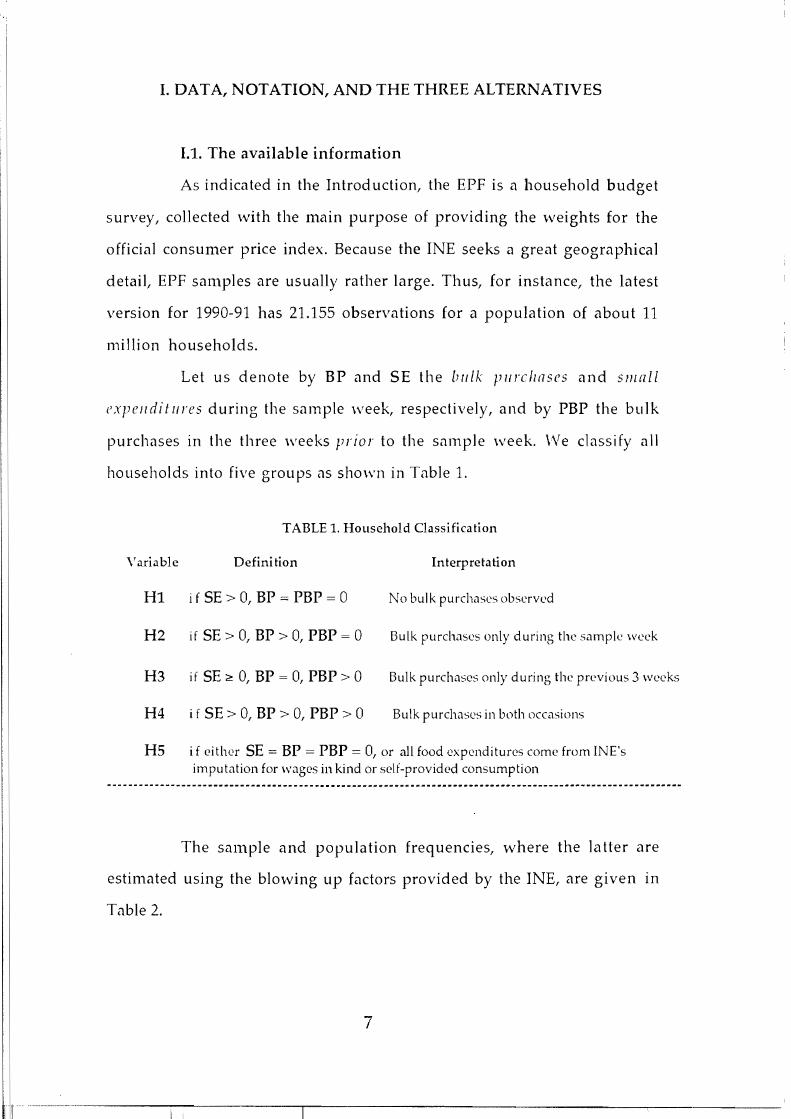
1.1. The available information

As indicated in the Introduction, the EPF is a household budget

survey, collected with the main purpose of providing the weights for the

official consumer price indexo Becuuse the INE seeks u greut geogruphical

detail, EPF samples are usually rather lurge. Thus, for instance, the latest

version for 1990-91 has 21.155 observutions for a population of about 11

million households.

Let us denote by BP and SE the lJIIlk pllrcJ¡l1ses und s}}lI1ll

expellditllres during the sample week, respeetively, and by PBP the bulk

purchuses in the three weeks prior to the sumple week. \Ve c1ussify ull

households into five groups us shown in Tuble 1.

TAnLE 1. Household Classification

\'ariable Defini tion Interpretation

H1 i f SE > 0, BP = PBP = ° No bulk purchases observed

H2 if SE> 0, BP > 0, PBP = ° Bulk purchases only during the sample week

H3 if SE ~ 0, BP = 0, PBP > ° Bulk purchascs only d uring the previous 3 weeks

H4 i f SE> 0, BP > 0, PBP > ° Bulk purchases in both occasions

H5 i f either SE = BP = PBP = 0, or all food expenditures come from lNE's imputation for wagcs in kind or sclf-providcd consumption

The sumple und population frequencies, where the latter are

estimated using the blowing up fuetors provided by the INE, are given 111

Tllble 2.

7

-----.------------;---------r----------------------....,--------­

---------------------------------------------------------------------

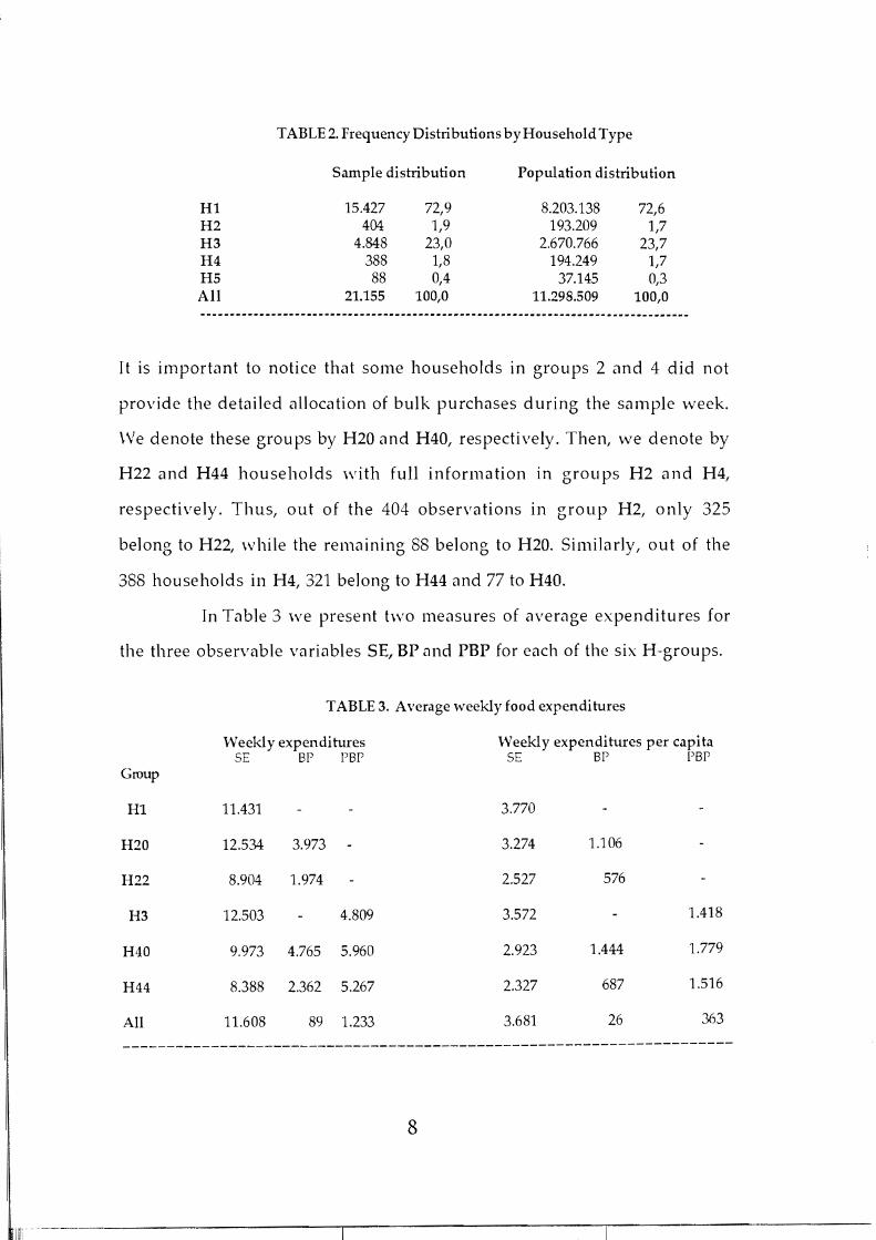
TABLE 2. Frequency Distributions byHousehold Type

Sample distribution Population distribution

Hl 15.427 72,9 8.203.138 72,6 H2 404 1,9 193.209 1,7 H3 4.848 23,0 2.670.766 23,7 H4 388 1,8 194.249 1,7 H5 AH

88 21.155

0,4 100,0

37.145 11.298.509

0,3 100,0

---------------------------.---.---.-._--------------------------------------------

It is import,mt to notiee that some households in groups 2 and 4 did not

provide the detailed alloeation of bulk purehases during the sample \Veek.

\Ve denote these groups by H20 and H40, respectively. Then, \Ve denote by

H22 <1nd H44 households with full information in groups H2 and H4,

respectively. Thus, out of the 404 observations in group H2, only 325

belong to H22, while the remaining SS belong to H20. Similarly, out of the

3SS households in H4, 321 belong to H44 <1nd 77 to H4ü.

In T<1ble 3 \Ve present two measures of <1verage expenditures for

the three observable variables SE, BP <1nd PBP for eaeh of the six H-groups.

TABLE 3. Average weekly food expenditures

Weeklyexpenditures Weekly expenditures per capitaSE sr psr SE sr PBr

Group

Hl 11.431 3.770

H20 12.534 3.973 3.274 1.106

H22 8.904 1.974 2.527 576

H3 12.503 4.809 3.572 1.418

H40 9.973 4.765 5.960 2.923 1.444 1.779

H44 8.388 2.362 5.267 2.327 687 1.516

AH 11.608 89 1.233 3.681 26

8

363

N otice the following three facts. In the first place, for both

groups which could not remember detail expenditures in their bulk

purchases d uring the sample week, namely groups H20 and H40, their BP

approximately doubles that magnitude for the groups with complete

information, namely groups H22 and H44, respectively. This might mean

that forgetful households tend to think that they spent more in bulk

purchases than households who keep good records of it.

In the second place, recall that the vast majority of H3

households are infrequent or occasional bulk purchasers. Therefore, their

PBP expenditures could be compared, to a first approximation, with the

corresponding magnitude for other households of that type, namely, BP

e:xpenditures for H20 and/or H22 hoseholds. Table 3 indica tes that the

group H3 is much closer on average to group H20. Therefore, we might

conjecture that, because of a certain idealization of the past, the bulk

purchases in group H3 are aIso exagerated.

In the third place, notice that groups H40 and H44 have their

PBP rather close to each other, contrary to their experience in BP which

was examined above. This might be the case because H44 househoIds tend

to suffer aIso from an idealization of the past effect.

1.2. The Poisson model for the frequency of purchase

\Ve do not have information about the household distribution

into the F(requent), 10(infrequent or occasional), and N(never) classes

defined in the Introduction. In order to obtain an estimate of such

distribution, we assume that the number of bulk purchases in a four week

period for people in classes F and 10 follows a mixed distribution a1PO"1) +

({2 P(I"2)' where al and a2 are the proportion of households in each group,

and PO) is a Poisson distribution with parameters Al (> 1) and )"2 « 1).

9

_..._-.__._--_.•_._------------,---------------------------­

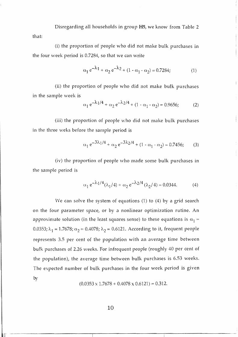
Disregarding aD households in group H5, we know frorn Table 2

that:

(i) the proportion of people who did not rnake bulk purchases in

the four week period is 0.7284, so that we can write

(ii) the proportion of people who did not rnake bulk purchases

in the sarnple week is

(iii) the proportion of people who did not make bulk purchases

in the three weks before the sample period is

(3)

(iv) the proportion of people who made sorne bulk purchases in

the sample period is

\Ve can solve the systern of equations (1) to (4) by a grid search

on the four pararneter space, or by a nonlinear optimization rutine. An

approximate solution (in the least squares sense) to these equations is al =

0.0353; )'1 = 1.7678; (X2 = 0.4078; )'2 = 0.6121. According to it, frequent people

represents 3.5 per cent of the population with an average time between

bulk purchases of 2.26 weeks. For infrequent people (roughly 40 per cent of

the population), the average time between bulk purchases is 6.53 weeks.

The expected number of bulk purchases in the four week period is given

by (0.0353 x 1.7678 + 0.4078 x 0.6121) = 0.312.

10

.-....-----.--------------r-------------~-_,__----.--------

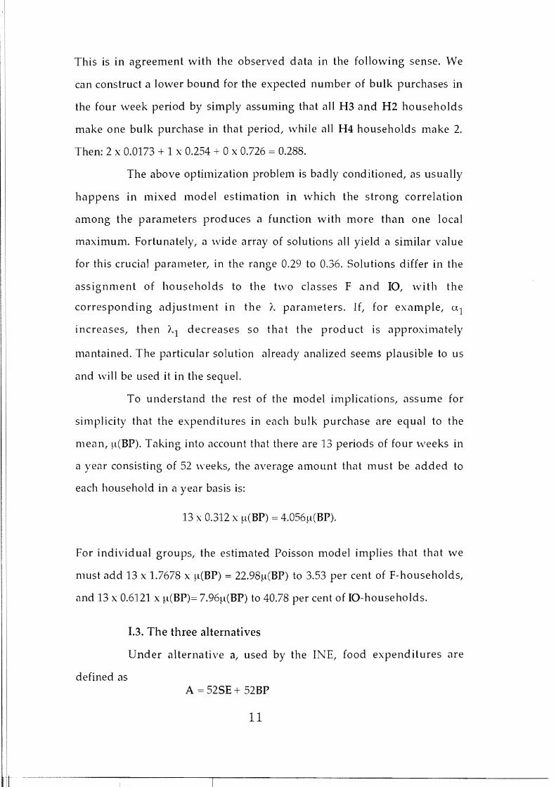
This is in agreement with the observed data in the following sense. We

can construct a lower bound for the expected number of bulk purchases in

the four week period by simply assuming that all H3 and H2 households

make one bulk purchase in that period, while all H4 households make 2.

Then: 2 x 0.0173 + 1 x 0.254 + Ox 0.726 = 0.288.

The aboye optimization problem is badly conditioned, as usually

happens in mixed model estimation in which the strong correlation

among the parameters produces a function with more than one local

maximum. Fortunately, a wide array of solutions all yield a similar value

for this crucial paral1leter, in the range 0.29 to 0.36. Solutions differ in the

assignment of households to the two classes F and lO, with the

corresponding adjustment in the 1, parameters. If, for exmnple, al

increases, then )'1 decreases so that the product is approximately

l1lantained. The particular solution already analized seems plausible to uS

and wil1 be used it in the sequel.

To understand the rest of the model implications, assume for

sil1lplicity that the expenditures in each bulk purchase are equal to the

mean, ~l(BP). Taking into account that there are 13 periods of four weeks in

ayear consisting of 52 weeks, the average amount that must be added to

each household in ayear basis is:

13 x 0.312 x ~l(BP) = 4.056~l(BP).

For individual groups, the estimated Poisson model implies that that we

must add 13 x 1.7678 x ~l(BP) = 22.98~l(BP) to 3.53 per cent of F-households,

and 13 x 0.6121 x ~l(BP)= 7.96~l(BP) to 40.78 per cent of 10-households.

1.3. The three alternatives

Under alternative a, used by the INE, food expenditures are

defined as A = 525E + 52BP

11

-~~_._~----------------¡-------------------------------

Information on PBP is ignored, but a weekly reference period is assigned to

BP. Apparently, the INE was interested in a rough approximation to the

average food expenditure per household for the population as a whole.

The implicit assumption is that, on average, the infravaluation of PBP for

H3 households will be offset by the overvaluation of BP for H2 and H4

households. However, as the INE is adding ~l(BP) per 0.034 household, this

implies an average of 52 x 0.034 x ~l(BP) == 1.768~l(BP). In other words,

alternative a is missing more than haH of the food expenditure increment

attributable to bulk purchases.

As far as different subgroups are concerned, \ve saw that the

Poisson model implies that we need to add 22.98~l(BP) to 3.53 percent of the

population and 7.96~l(BP) to 40.78 per cent of the population, whereas

alternative a is simply adding 52~l(BP) to 3.44 percent of H2 and H4

households. In brief, this procedure i) underestimates heavily for the

population as a whole, and ii) overestimates for a large amount a small

percentage of the population.

Under alternative b,only SE expenditures are assigned a weekly

reference period, while aggregate bulk purchases are assigned a four \veek

reference periodo Therefore, annual food expenditures are now

B == 52SE + (BP + PBP)13.

lt is not possible to know a priOri if this alternative over or

underestimates on average on each of the groups. We do know that B == A

for Hl, B < A for H2, B > A for H3, and B can be greater or smaller than A

for H4.

From Tables 2 and 3 we obtain that ~l(PBP) == 1.876~l(BP).

Therefore, this proced ure is adding on average an addi tional food

expenditure of

12

"--------'-------------,-------------,--------------­

i '1

[O.Ol71~l(BP) + 0.2372~l(PBP) + 0.0173Ül(BP) + ~l(PBP))]13 = 6.65~l(BP) (5)

Thus, alternative b overestimates total expenditure by rougly 50 per cent.

Of course, as under alternative a, the unobserved percentage of infrequent

households in group Hl are necessarily undervalued. \Vith this approach,

we are adding 24.39~l(BP) to the 23.72 percent of the population in group

H3, and 13 x 2.876~l(BP) = 37.39~l(BP) to 1.8 percent of the population in

group H4. According to the Poisson model, we need to add 7.96~l(BP) to

40.78 percent, and 22.98~l(BP) to 3.53 percent. This suggests that groups H3

and H4 are probably overvaluated. ivloreover, as these two groups receive

all the additions, group H2 is expected to be lIndervalllated on average,

since no increment is applied to it.

Our third procedure seeks to add an average expenditure to

match the expected estimated vallle. This implies a change in the

frequency in (5) sllch that

[0.0171 ~l(BP) + O.2372~l(PBP) + O.0173Ül(BP) + ~l(PBP»] y = 4.056~l(BP).

Taking into account that ~l(PBP) = 1.876~l(BP), we find that y = 7.924, instead

of 13. This means that we are adding an average amount of 22.79~l(BP) to

1.73 per cent of frequent households in H44, 7.924~l(BP) to a small group of

infrequent households in H2, representing 1.71 per cent of the population,

and 14.86~l(BP) to H3 households wich constitute 23.72 percent of the

population.

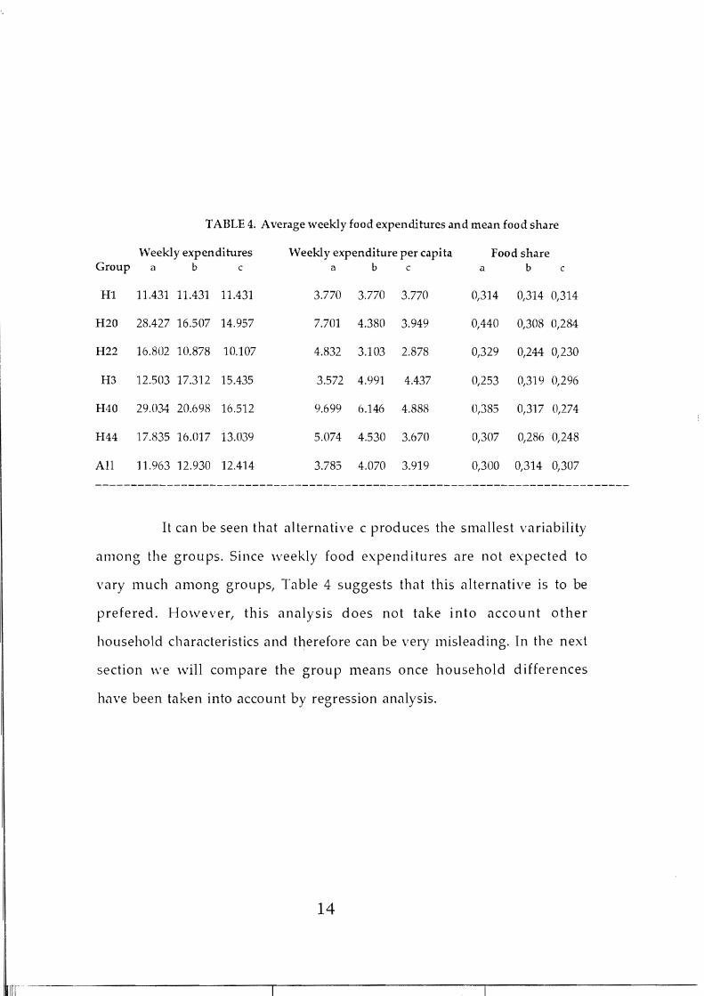
For comparison purposes, in Table 4 we present average weekly

expenditures, weekly expenditures per capila and the share of total

expenditures devoted to food for aH groups and the population as a whole

lInder the three options.

13

-----------------,--------------.--------------­

I I

---------------------------------------------------------------------------

TABLE 4. Average weekly tood expenditures and mean tood share

Weeklyexpenditures Weekly expenditure per capita Food share Group a b e a b e a b e

Hl 11.431 11.431 11.431 3.770 3.770 3.770 0,314 0,314 0,314�

H20 28.427 16.507 14.957 7.701 4.380 3.949 0,440 0,308 0,284�

H22 16.802 10.878 10.107 4.832 3.103 2.878 0,329 0,244 0,230�

H3 12.503 17.312 15.435 3.572 4.991 4.437 0,253 0,319 0,296�

H40 29.034 20.698 16.512 9.699 6.146 4.888 0,385 0,317 0,274�

H44 17.835 16.017 13.039 5.074 4.530 3.670 0,307 0,286 0,248�

All ]1.963 ]2.930 ] 2.414 3.785 4.070 3.919 0,300 0,314 0,307�

It can be seen that alternative c produces the smalIest variability

among the groups. Since weekly food expenditures are not expected to

vary much among groups, Table 4 suggests that this aIternative is to be

prefered. However, this analysis does not take into account other

household characteristics and therefore can be very misleading. In the next

section we will compare the group rneans once household differences

have been taken into account by regression analysis.

14

11. REGRESSION ANALYSIS�

11.1. First set of results for the three alternatives

Our first task, is to place the previous discussion in a multiple

regression setting. Following Deaton et al (1989), we select a flexible

functional form for the food share equation. Taking INE's as the reference

option, we have

SHA == AlTEA = a + ~ ln(PCTE) + Aln(HS) + LjojNj + y Z + E, (6)

where: - TEA is household total expenditure when food expenditure is

equal to A;

- HS is household size;

- PCTE == TEA/HS is per capita household total expenditure;

- Nj == HSj/HS, and HSj is the number of household members in

jth's age bracket;

- z is a vector of explanatory variables which are identified in the

Appendix.

Although (6) can be given a formal interpretation in utility

theory, we regard the equation as a convenient representation of the

expectation of food patterns conditional on the explanatory variables. The

starting point for (6) is Working's (1943) Engel curve study, which linearly

relates the share of expenditure on each good to the logarithm of per capita

total expenditure. Here the effects of household composition are modeled

by the inclusion of the logarithm of household size, lnHS, together with

the ratios H5jl H5 to capture the additional effects of composition.

To this model, we add up a set of dummy variables Hi, where i =

20, 22, 3, 40 Y44, to capture the effect of belonging to any of these groups

relative to the reference group Hl. For each of the H groups, descriptive

statistics for selected variables entering the regression analysis are included

15

III--------------------r----------------------­

in the Appendix. In Table 5 we present the coefficient estima tes for the

variables we are more interested in (with t-values between brackets), total

expenditure elasticities, and a measure of the goodness of fit.

TABLE 5. Summary of regression results for different options

Option a Option b Option e INTERCEfYf 1.7191 (75.1) 1.8269 (79.5) 1.7999 (79.2) H3 -0.0201 (-10.9) 0.0580 (31.4) 0.0298 (16.3) H20 0.1664 (13.6) 0.0121 (1.0) -0.0158 (-1.3) H22 0.0524 (8.1) -0.0453 (-7.1) -0.0614 (-9.6) H40 0.1718 (12.4) 0.0969 (7.1) 0.0454 (3.3) H44 0.0505 (8.1) 0.0284 (4.6) -0.0164 (-2.6) InPCTE -0.1022 (-61.9) -0.1097 (-66.3) -0.1079 (-65.R) Elasticity 0.6597 0.6504 0.6487

R2 0.4054 0.4027 0.4041 Samplc sizc 21.063 21.067 21.067

The following comments are in order:

i) The complete model for alternative c appears as Model 1 in

the Appendix, \vhere the results are briefly discussed. Detailed results for

alternatives a and b are very similar and will be provided upon request. In

any case, the goodness of fit for all options is satisfactory for this large

cross-section. Heteroskedasticy was much improved by the logarithmic

transformation of pe/' capila total expenditure.

ii) For the sample as a whole, food is clearly a necessity, with a

total expenditure elasticity of approximately 0.65 under all options.

iii) As expected, H3 households appear undervalued in option a

which does not give any weight to PBP. On the contrary, since BP are

treated as weekly expenditures, groups 20, 22, 40 and 44 appear very

significantly overvalued. Households in H20 and H40, who do not register

their <llloc<ltion of bulk purch<lses to specific commodities, seem to

eX<lggerate the amount spent on food, a fact already apparent in Table 3.

Consequently, they appear as particularly overvalued under option a.

16

._----------_._--------,.-----------------,-------------­

iv) \Vith regard to option b, as expected H3 and H4 households

are, on average, overvalued. However, the amount of overvaluation is

between one haH and one third that of H20 and H40 under a. Group H22 is

now significantIy undervalued. Taking into account Table 3, we conjecture

that this type of infrequent households spent less than usual on minor

weekly items because they were under the shock of a contemporaneous

bulk purchase d uring this same sample week. A1though a similar

phenomenon must be present among H40 households, they are known to

have an upward bias in their bulk purchases during the sample week. At

any rate, H40 and H44 hOllseholds are overvalued, but about haH than

under alternative a. Finally, note that, as expected, the intercept is larger in

b than in a because the overall underestimation is smaller.

v) Option c values BP and PBP less than option b.

Correspondingly, H4ü hOllseholds are much less overvalued and H44 are

now slightly below the reference group. lnfrequent H2ü households

remain essencially insignificant, but with a minus sign, while the H22

group appear heavily undervallled. Possibly the best feature of this option

",ith respect to option b is that the large group of H3 hoseholds is now

l1luch less overvalued.

11.2. Correction for outliers

\Ve have seen how a priori considerations on under and

overval uation caused in each of the three alternatives were confirmed by

the regression analysis. Therefore, we have grounds to select those outliers

which can be attributed to imperfect imputation of bulk purchases. The

aim would be to correct them on an individual basis to reach a second,

presumably improved version of each alternative.

However, before proceeding in this direction we must check

whether sorne outliers could be explained by other factors. In particular,

17

._._.._---------------,--------------------------­

the INE performs imputations to subsidized meals at work, and to meals

in the household owned restaurant. We find that 23 negative outliers

have a low food share beeause they have a signifieant imputation of either

of these two types. These observations are not eorreeted, but taken apart in

group H5 in order not to influenee the analysis in the sequel.

Suppose that we fit a multiple regression model to a set of n

observations in whieh there exists a subset of nO observations

undervaluated, that is, the observed response value at these nO points is

yob = Yrea1 - k¡,

where k¡ > O. Assuming that the undervaluation oeeurs randomly and it is

110t related to the vector of explanatory variables, it is straightforward to

show that the expeeted effeet of these outliers is to bias the intereept by

k*(no/n), where k* = (L¡k¡)/no' Therefore, if we fit the regression models

given in (6) without the H dummy variables, we expeet to find in eaeh

group outliers with the opposite sign that the sign of the dummy variable

in the group (see Table 5 for the latter). Sinee group Hl may be

underval uated in the three alternatives, we can assume that large negative

outliers in that group are due to the underestimation of bulk purehases.

The seareh for outliers is earried out by the proeedure of Peña

and Yohai (1995), that has proved to be able to identify groups of outliers

avoiding the masking effect. The outliers are testeq with a eritieal value for

te studentized residual of 5. This high value has beeen ehosen beeause (i) it

is required to avoid eorreetion for small effects, beeause as explained before

the bias of the intereept may lead to a biased estimation; (ii) outliers due to

to awrong imputation for bulk purehases are expected to be large, and (iii)

the sample size is large. With this proeedure, those outliers attributable to

wrong bulk purehase imputations for alternatives a and e, are shown in

Table 6.

18

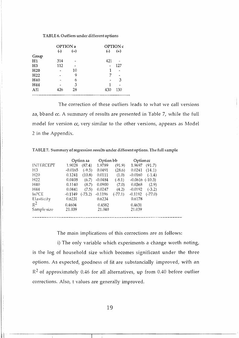
TABLE 6. Outliers under different options

OPTIONa OPTIONc (-) (+) (-) (+)

Group Hl 314 421 H3 112 - 127 H20 10 1 H22 9 7 H40 6 3 H44 3 1 Al! 426 28 430 130

The correction of these outliers leads to what we call versions

aa, bband ee. A summary of results are presented in Table 7, while the full

model for version ee, very sin'lilar to the other versions, appears as Model

2 in the Appendix.

TAfiLE 7. Summary of regression results under different options. The ful! sample

Option aa Option bb Optioncc INTERCEPT 1.9028 (87.4) 1.9789 (91.9) 1.9697 (91.7) H3 -0.0165 (-9.5) 0.0491 (28.6) 0.0241 (14.1) H20 0.1241 (10.8) 0.0111 (1.0) -0.0160 (-1.4) H22 0.0408 (6.7) -0.0484 (-8.1) -0.0616 (-10.3) H40 0.1140 (8.7) 0.0900 (7.0) 0.0368 (2.9) H44 0.0441 (7.5) 0.0247 (4.2) -0.0192 (-3.2) InPCE -0.1149 (-73.2) -0.1196 (-77.1) -0.1192 (-77.0) Elasticity 0.6231 0.6234 0.6178

R2 0.4604 0.4582 0.4631 5,1mplc sizc 21.039 21.040 21.039

The main implications of this correetions are as follows:

i) The only variable whieh experiments a ehange worth noting,

15 the log of household size whieh beeomes signifieant under the three

options. As expected, goodness of fit are substancíally improved, with an

R2 of approximately 0.46 for aH alternatives, up from 0.40 before outlier

corrections. Also, t values are generalIy improved.

19

ii) Tot(ll expenditure el(lstieity for the full s(lmple goes down,

(lpproxim(ltely, from 0.65 to 0.62 in (lll (lltern(ltives.

iii) In option aa, H3 households (lppeJr still signifie(lntly

underv(llued (lfter the tre(ltment of outliers, while all the rest, speeially

groups H20 (lnd H40, rem(lin seriously overv(llued.

iv) In option fu we observe (l c1eJr improvement of the

overv(llu(ltion of H44 (lnd H3 households. Nevertheless, there remains

the l(lrge overvaluation of group H40 and the underv(lluation of

infrequent households in H22.

v) In option ce the lJrge group H3 has improved eonsider(lbly

respect option fu, (lnd it is nm'\' of the S(lme order of m(lgnitude but

opposite sign rel(ltive to aa. In (lbsolute terms, option ce domin(ltes c1e(lrIy

(lltern(ltive aa for H20, H40 (lnd H44 households, (lnd performs \\'orse on ly

for group H22 \\'hich seems to rem(lin underv(llued.

20�

111. IMPLICATIONS

Once we have made the best we could with the available

information, it is time to explore the conseguences of choosing version cc

rather than sticking to INE's option a.

111.1. The impact on the measurement of inflation

We have measured the inflation for the food (drinks and

tobacco) category during 1993 and 1994 under both alternatives. For that

purpose, we ha ve constructed a Laspeyres type price index for the

population as a whole (including from Hl to H5 households).

Let Ah be the food expenditure of household h under

alternative a, for example, and let W~1 be the share of Ah (net of the 25th

item of lInclassifiable expenditllres) devoted to food item i. Let W =

(\V1, ... ,\V24) be the 24 dimensional vector of poplllation shares, where, for

each i, \Vi is the weighted mean of the w~'s, with weights egual to the

A h 's. Then the index we use to compare the price vector Pt with base

. . pnces Po lS

Under the current Consumer Price Index system, based in 1992, the INE

publishes monthly data for the ratios (Pti/pOi)' The vector W under

alternative a is essentially the vector used in the official system. The

constrllction of such vector under alternative ee is described in the

Appendix.

The results are as follows. Option a yields a food price index of

102.38 and 108.22 for 1993 and 1994, respeetively. Option ee yields 102.40

(Ind 108.24, a small difference indeed.

21

-----"----------------r----------------------------­

On the other hand, notice that the share of household total

expenditure devoted to food is 0.2996 and 0.3108 for options a and cc,

respectively. Not a large difference either. Therefore, we should not expect

great differences in the general price index, covering food and the other

eight commodity categories. Indeed, under option a our estimates for the

general price index are 105.25 and 110.23 for 1993 and 1994, respectively,

while under alternative cc they are 105.24 and 110.22 for those same years.

11I.2. The impact on the measurement of inequality

To take into consideration different household needs arising

from a different household size, sh, under alternative a, for example,

define adjusted food expenditure by

\Ve have selected the polar cases 8 = Oand 8 = 1, corresponding to original

househoJd food expenditure, andpcr capila household food expenditure,

respectiveJy. \Ve ha ve chosen also the case 8 = 0.5, corresponding to an

intermediate víe,\' about the importance of economies of scale in

consu mption within the hOllsehold.

Becallse of its good properties(2), \Ve have considered the

generalized entropy family of relative ineqllality indices: ,

Ic(z) = (1/H)[l/ c(c -l)J[Ih (zh hl(Z))C - 1], c ;é 1, O;

c = 1;

c = O,

where ~l is the function providing the distribution mean. In particular, we

have selected a member of this family more sensitive to the upper part of

the distribution, c = 2 -which is 1/2 the coefficient of variation- and a

member more sensitive to the lower part, c = -1. \Ve have estimated also

22

!'

the two indiees origina11y suggested by Theil eorresponding to e = 1 and e =

O.

The results are in the left hand side of Table 8. \Ve observe a

systematie improvement in food expenditure inequality with option ce for

a11 values of e and a11 members of the generalized entropy family. The

estimated reduetion of inequality ranges from a minimum of 12 pereent to

a maximum of 50 pereent. Sueh an improvement is greater the more

sensitive one is to the upper tail of the distribution, and at an intermedia te

value of the parameter representing the importanee of eeonomies of seale.

Finally, \Ve have earried on the same exereise for the

distribution of total expenditure. The results are in the right hand side of

Table S. The improvement in inequality persists in this domain, but loses

importanee: the range of variation is from 1.5 to 3.0 pereent.

TABLE 8. Inequality under different options

Food expenditure inequality Total expenditure inequality

e = 0.0 e =2 e=l e=O e =-1 e =2 e=l e=O e =-1

Option a 0.1813 0.1636 0.1853 0.3163 0.2525 0.2046 0.2169 0.3089

Optionee 0.1613 0.1463 0.1593 0.2185 0.2474 0.2021 0.2134 0.2994

alce 1.1240 1.1182 1.1632 1.4476 1.0206 1.0123 1.0164 1.0317

e = 0.5

Option a 0.1412 0.1249 0.1341 0.1982 0.2128 0.1701 0.1697 0.2111

Optionee 0.1208 0.1066 0.1089 0.1308 0.2094 0.1674 0.1664 0.2043

alce 1.1689 1.1717 1.2314 1.5145 1.0162 1.0161 1.0198 1.0333

23

._--------.-------------¡--------------------------­

e = 1.0

Option a 0.1726 0.1414 0.1423 0.1887 0.2575 0.1922 0.1831 0.2179

Optionee 0.1497 0.1224 0.1184 0.1349 0.2535 0.1894 0.1800 0.2123

a/ee 1.1530 1.1552 1.2018 1.3988 1.0158 1.0148 1.0172 1.0264

24�

: I

NOTES�

O) See Pudney (987) and Meghir and Robin (992), and the

references quoted there.

(2) For a characterization, see for instance Shorrocks (980). For a

defense, discussion and applications, see Cowell (984), Coulter el al 0992a,

1992b), and Ruiz-Castillo (1995).

25

---_.-.--------------.--_._------------------------­

REFERENCES�

Coulter, F., F. Cowell and S. Jenkins (1992a), "Differences in Needs

and Assessment of Income Distributions," BlIlletill 01 ECOIlOllzic Research,

44: 77-124.

Coulter, F., F. Cowell and S. Jenkins (1992b), "Equivalence Scale

Relativities and the Extent of Inequality and Poverty," EcollolI/ic TOllnzal,

102: 1067-1082.

Cowell, F. (1984), "The Structure of American Income lnequality,"

Rn)icw 01 ll1colI/c alld Wcalth, 30: 351-375.

Deaton, A., J. Ruiz-Castillo and D. Thomas (1989), "The Influence

of Household Composition on Household Expenditure Patterns: Theory

and Spanish Evidence," TOl/mal 01 Political EcollolI/Y, 97: 179-200.

t"leghir, C. and J. M. Robin (1992), "Frequency of Purchase and the

Estimation of Demand Systems",jol/nU7l 01 EcollolI/etrics, 53: 53-86

Peila, D. and V. Yohai (1995), "The Detection of Influentia! Subsets

in Linear Regression by Using an Influence Matrix", TOl/mal 01 the Royal

Statistiwl Society, Serie B. 57: 1-12.

Pudney, S. (1987), "On the Estimation of Engel Curves", presented

at a CO/llerellce 011 Mea5l1rell/ellt alld Modellillg ill ECOll01llics, Nuffield

College.

26

"'----'---'-----------,-----------------------­

Ruiz-Castíllo, J. (1995), "The Anatomy of Money and Real

Inequality in Spain, 1973-74 to 1980-81", forthcoming in JOlmzal 01 Illcome

Distriblltioll, 4.

Shorrocks, A. (1980), "The Class of Additively Decomposable

Inequality Measurements," Ecollollletrica, 48: 613-625.

\Vorking, H. (1943), "Statistical Laws of Family Expenditure,"

JOl/mal 01 tire A1I1eriCl7J1 Statistical Associatioll, 38: 43-56.

27

.- ......-.----------------T------------------------.

APPENDIX�

I. VARIABLES DEFINITION

Demographic

HS = household size

Nj = HSj/HS, where� HSl = number of household members less than 4 years old HS2 = number of household members between 4 and 8 years old HS3 = number of household members between 9 and 14 years old HS4 = number of household members between 15 and 17 years old HSS = number of household members between 18 and 24 years old HS6 = number of household members between 25 and 40 years old HS7 = number of household members between 41 and 64 years old HS8 = number of household members between 65 and 75 years old HS9 = number of household members older than 75 years

Socioeconomic

N"EARN = number of income earners in the household

s = female household head

HHEDl = household head educational level: illiterato� HHED2 * = without formal studies or only first grade� HHED3 = second grade� HHED4 = high school� HHED5 = three year college degree� HHED6 = other college degrees and graduate studies�

SEDO = no espouse SEDl * = espouse educationallevel: illiterate, without formal studies, first and second grade SED2 = high school SED3 = college degree and graduate studies

SOCIal = agrarian worki ng class, and smalllandowners SOCI02 * = non-agricultural working class and other unclassifiable mc'mbers of the labor force SOCI03 = agrarían entrepeneurs, armed forces, non-agrarían entrep. without salaried workers SOCI04 = middle and upper class SOCIOS = not in the labor force

l\IIGR= recently inmigrated household head

Housing condi tions

50:\1 = housing living space in square meters

TENl * = owner-occupied housing� TEN2 = market rental housing� TEN3 = subsidized public housing� TEN"4 = rental housing, unknown legal condition� TEN5 = other housing tenure�

BUILDl * = detached, single housing unit� BUILD2 = building with two housing units�

28

------------------------,------------------------------­

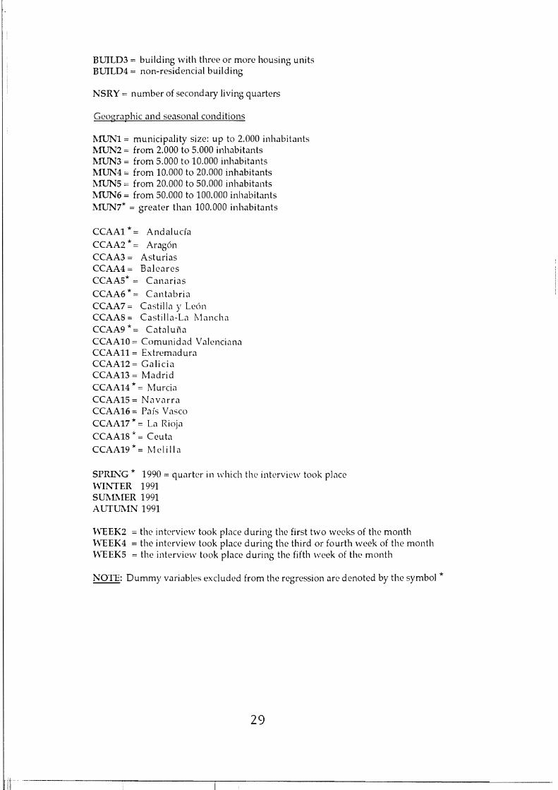
BUILD3 = building with three or more housing units BUILD4 = non-residencial building

NSRY = number of secondary living quarters

Geographic and seasonal conditions

l\1UNl = municipality size: up to 2.000 inhabitants l\1UN2 = from 2.000 to 5.000 inhabitants l\1UN3 = from 5.000 to 10.000 inhabitants MUN4 = from 10.000 to 20.000 inhabitants l\1UN5 = from 20.000 to 50.000 inhabitants l\1UN6 = from 50.000 to 100.000 inhabitants l\1UN7* = greater than 100.000 inhabitants

CCAAl *= Andalucía

CCAA2 * = Aragón CCAA3 = Asturias CCAA4 = Baleares CCAA5* = Canarias

CCAA6 * = Cantabria CCAA7 = Castilla y León CCAA8 = Castilla-La Mancha CCAA9 * = Cataluña CCAA10 = Comunidad Valenciana CCAAll = Extremadura CCAA12 = Galicia CCAA13 = Madrid CCAA14 * = Murcia CCAA15 = Navarra CCAA16= País Vasco CCAA17 * = La Rioja CCAA18 * = Ceuta

CCAA19 * = Melilla

SPRING * 1990 = quarter in which the interview took place \VII\,TTER 1991 SUMl\1ER 1991 AurUl\1N 1991

WEEK2 = the interview took place during the first two weeks of the month WEEK4 = the intervicw took place during the third or fourth week of the month WEEK5 = thc intervicw took place during thc fifth weck of the month

NOTE: Dummy variables exc!uded from the rcgression are denotcd by the symbol *

29

...._---------_._----:-------¡-------------------------­

n. DESCRIPTIVE STATISnCS

Mean of selected continous variables

Hl H2 H3 H4 AH TE 2.198.608 2.704.966 3.137.648 3.227.491 2.447.747 HS 3,27 3,84 3,77 3,83 3,41 PCTE 737.321 766.088 907.804 936.648 781.685 SQM 102.0 100.2 107.2 107.7 103.3

Percentage distributions of selected discrete variables

NSRY O 89,9 90,4 86,3 89,9 89,1 1 9,8 9,0 13,1 10,1 10,5

2ormore 0,3� MM -º'-º­100,0 100,0 100,0 100,0 100,0

NEARN O 0,06 0,04 1 43,3 40,4 38,1 35,3 41,9

2ormore� 56,64 59,6 61,9 64,7 58,06 100,00 100,0 100,0 100,0 100,00

HHED 1 5,4 2,3 1,7 2,4 4,4 2 63,9 50,3 49,0 43,8 59,7 3 15,2 20,7 19,1 18,0 16,3 4 8,4 16,4 15,3 18,7 10,4 5 3,8 5,9 6,8 7,4 4,6

9,76 3,3 ----.1A JU ~ 100,0 100,0 100,0 100,0 100,0

SOCIO 1 7,8 8,4 5,0 3,4 7,1 2 21,3 27,7 26,4 25,3 22,7 3 20,5 24,5 28,8 28,3 22,6 4 8,7 13,1 15,6 21,1 10,6 5 41,7 26,3 24,2 21,9 37,0

100,0 100,0 100,0 100,0 100,0

l\IUN 1 8,2 7,0 4,6 3,9 7,3 2 9,7 6,2 5,8 5,0 8,6 3 11,6 7,6 8,5 6,2 10,7 4 10,9 9,9 8,9 8,3 10,4 5 12,2 7,2 10,5 7,6 11,6 6 8,7 9,6 9,7 7,7 9,0 7 38,7 52,5 52,0 61,3 42,4

100,0 100,0 100,0 100,0 100,0

30

....__._--------------,-------------------------­

------------------------------------------------------

III. REGRESSION RESULTS

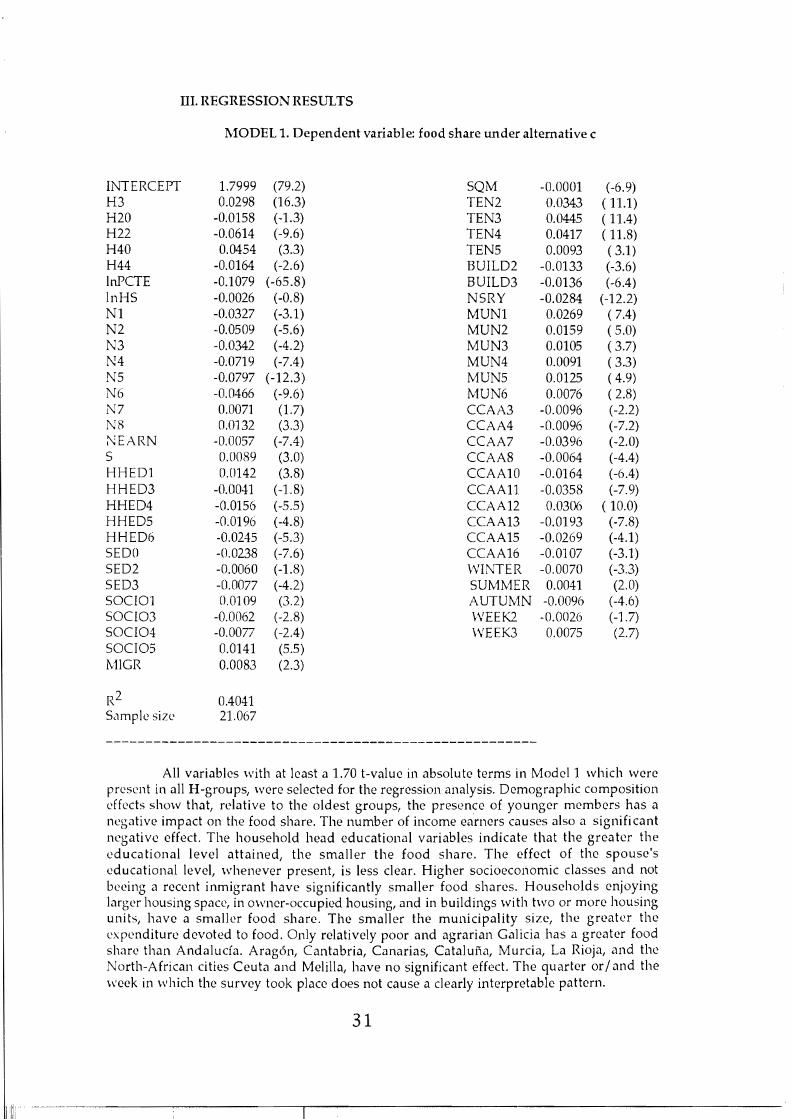
MODEL 1. Dependent variable: food share under altemative e

INTERCEPT 1.7999 (79.2) SQM -0.0001 (-6.9) H3 0.0298 (l6.3) TEN2 0.0343 (11.1) H20 -0.0158 (-1.3) TEN3 0.0445 (11.4) H22 -0.0614 (-9.6) TEN4 0.0417 ( 11.8) H40 0.0454 (3.3) TEN5 0.0093 ( 3.1) H44 -0.0164 (-2.6) BUIlD2 -0.0133 (-3.6) InPCTE -0.1079 (-65.8) BUIlD3 -0.0136 (-6.4) InHS -0.0026 (-0.8) NSRY -0.0284 (-12.2) NI -0.0327 (-3.1) MUN1 0.0269 ( 7.4) N2 -0.0509 (-5.6) MUN2 0.0159 ( 5.0) N3 -0.0342 (-4.2) MUN3 0.0105 ( 3.7) N4 -0.0719 (-7.4) MUN4 0.0091 ( 3.3) N5 -0.0797 (-12.3) MUN5 0.0125 ( 4.9) N6 -0.0466 (-9.6) MUN6 0.0076 ( 2.8) N7 0.0071 (l.7) CCAA3 -0.0096 (-2.2) N8 0.0132 (3.3) CCAA4 -0.0096 (-7.2) :\'EARN -0.0057 (-7.4) CCAA7 -0.0396 (-2.0) S 0.0089 (3.0) CCAA8 -0.0064 (-4.4) HHEDl 0.0142 (3.8) CCAA10 -0.0164 (-6.4) HHED3 -0,(1041 (-1. 8) CCAAll -0.0358 (-7.9) HHED4 -0.0156 (-5.5) CCAA12 0.0306 ( 10.0) HHED5 -0.0196 (-4.8) CCAA13 -0.0193 (-7.8) HHED6 -0.0245 (-5.3) CCAA15 -0.0269 (-4.1 ) SEDO -0.0238 (-7.6) CCAA16 -0.0107 (-3.1 ) SED2 -0.0060 (-1.8) WINTER -0.0070 (-3.3) SED3 -o.oon (-4.2) SUMMER 0.0041 (2.0) SOCIOl o.m 09 (3.2) AUTUMN -0.0096 (-4.6) SOCI03 -0.0062 (-2.8) WEEK2 -0.0026 (-1.7) SOCI04 -0.0077 (-2.4) WEEK3 0.0075 (2.7) SOCIOS 0.0141 (5.5) MIGR 0.0083 (2.3)

R2 0.4041 S.1mplc size 21.067

All variables with at 1east a 1.70 t-value in absolute terms in Model 1 which were present in all H-groups, were selected for the regression analysis. Demographic composition dfccts show that, rc1ative to the oldest groups, the presence of younger members has a negative impact on the food share. The number of income earners causes also a significant ncgativc effect. The household head educational variables indicate that the greatcr the cducational level attained, the smaller the food share. The effect of the spouse's cducational level, whenever present, is less clear. Higher socioeconomic classcs and not bccing a reccnt inmigrant have significantly smaller food sharcs. Households enjoying largcr housing spacc, in owner-occupied housing, and in buildings with two or more housing units, have a smallcr food share. The smaller the municipality sizc, the grcatcr thc expcnditurc devoted to food. Only relatively poor and agrarian Galicia has a greatcr food sharc than Andalucía. Aragón, Cantabria, Canarias, Cataluña, Murcia, la Rioja, and the North-African citics Ceuta and Melilla, have no significant effect. The quarter or / and the week in which the survey took place does not cause a clearly interpretable pattern.

31

MODEL 2. Dependent variable: food share under altemative ee

INTERCEPT 1.9697 (91.7) SQM -0.0001 (-7.7) H3 0.0241 (14.1 ) TEN2 0.0348 ( 12.1) H20 -0.0160 (-1.4) TEN3 0.0427 ( 11.7) H22 -0.0614 (-10.3) TEN4 0.0410 ( 12.4) H40 0.0368 (2.9) TEN5 0.0109 ( 4.0) H44 -0.0192 (-3.3) BUlLD2 -0.0151 (-4.4) InPCTE -0.1192 (-77.0) BUlLD3 -0.0140 (-7.0) InHS -0.0145 (-4.6) NSRY -0.0265 (-12.2) NI -0.0306 (-3.1) MUN1 0.0148 ( 5.0) N3 -0.0302 (-3.9) MUN3 0.0119 ( 4.4) N4 -0.0706 (-7.8) MUN4 0.0083 ( 3.2) N5 -0.0755 (-12.5) MUN5 0.0122 ( 5.1) N6 -0.0521 (-11.5) MUN6 0.0102 ( 3.9) N7 0.0047 (1.2) CCAA3 -0.0099 (-2.4) N8 0.0109 (2.9) CCAA4 -0.0376 (-7.3) NEARN -0.0049 (-4.9) CCAA7 -0,(l073 (-2.5) S 0.0028 (1.0) CCAA8 -0.0185 (-5.3) HHED1 0.0165 (4.7) CCAA10 -0.0178 (-7.3) HHED3 -0.0043 (-2.0) CCAAll -0.0432 (-10.3) HHED4 -0.0134 (-5.1 ) CCAA12 0.0337 ( 11.8) HHED5 -0.0201 (-5.3) CCAA13 -0.0187 (-8.1) HHED6 -Cl.0243 (-5.7) CCAA15 -0.0265 (-4.3) SEDO -0.0175 (-6.0) CCAA16 -0.0102 (-3.2) SED2 -0.0020 (-0.6) WINTER -0.0070 (-3.6) SED3 -0.0140 (-3.5) SUMMER 0.0042 (2.2) SOCI01 0.Cll03 (3.2) AUTUMN -0.0096 (-4.6) SOCI03 -0.0058 (-2.8) WEEK2 -0.0026 (-1.8) SOCI04 -0.0047 (-1.5) WEEK3 0.0062 (2.4) SOCI05 0.0131 (5.5) MIGR 0.0081 (2.4)

R2 0.4631 Sample size 21.039

The most important difference is in the coefficient of the log of household size, InHS, which is now clearly significant and it was not before. Not having a spouse, or having one highly educated, depresses the food share. AH other patterns present in Model 1 are maintained, although four variables -N7, S, SED2 and SOCI04- are no longer significant.

32�

IV. ALLOCATION

In option e we have made the best possible imputation of annual food expenditures from the available information d uring a four week observation periodo However, for H20 and H40 households bulk purchases made during the sample week must be allocated among the 25 specific food items. The same must be done for bulk purchses during the prior three weeks for H3 , H40 and H44 households.

We start from the hypothesis that people might not buy goods in the same proportion in a bulk purchase, possibly in a large discount store in a shopping mall, than in smaller acquisitions during weekly errands in their neighbourhood. We have complete information in this respect for H22 and H44 households. Based on the shopping behavior of these groups, we have classified 25 commodities into bulk purchase-goods, weekly-goods, and other-goods. For every i = 1,..., 25, let us denote by BPW¡ and SEW¡ the share of BP and

SE expenditures, respectively, devoted to good i. Whenever the variable (BPW¡ - SEW¡)

takes a sizable positive value for both H22 and H44 households, we say that good i is a bulk purchase-good. Whenever it takes a negative value for both groups, we say that it is a H'eekly-good. lf this variable takes small values andj or different signs depending on the group, then we classify it as an other-good.

Following this criterion, we partition the set into 9 bulk purchase-goods, 8 weekly­goods, and 8 other-goods. This is a reasonable classification: i) prepared goods of all sorts appear prominently in bulk purchases; ii) all types of fresh items appear as weekly goods; iii) different meats, milk, both alcoholic and non-alcoholic drinks, as well as tobacco which is only bought in special stores, appear as neither and form a group of its own.

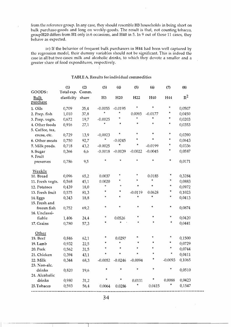
In the next step, befare deciding on an allocation procedure for the aboye household groups, we would like to lcarn as much as possible about their behavior in this 25­dimensional cornmodity space. Of course, at this level of dctail, for households in groups Hl, H3, H20, and H40 we have only information on SE expenditurcs. Nevcrthcless, we run two types of rcgressions for thc sample of 21.039 observations remaining after the outliers analysis Icading to option 0:. In thc first place, we run 25 regressions to compute total cxpenditure clasticities for cach good. These are prcsented as column (1) in Tablc A. In the second place, w~ run 25 regressions to explain the allocation of aggregate food expenditure under alternative e to the 25 food commodities. Per thousand commodity shares, as a pro portian of aggregate food expenditures, are presented in column (2) in Table 10. Regression coefficients for the 5 groups, relative to the Hl reference group, are presented in columns (3) to (7). Non significant coefficients are singled out by means of an arterisk.

Finally, each equation's R2 is provided in column (8).

i) Wc are mostly interested in learning as much as possible about the largest of alJ difficult groups, namely, H3 households. These households, who were observed to make sorne bulk purchase only during the three weeks prior to the sample week, contain a large proportion of people who rnakc a bulk purchasc every four weeks or more. Given the aboye classification, we expect them to be short of bulk purchase-goods, long on weekly-goods, and close to the reference group in other-goods. Non counting tobacco, H3 households satisfy the expected pattern in 13 cases, present a single violation in other-goods, and non significant coefficients in the remaining 10 cases.

ii) lt is illuminating to compare this evidence with the case of infrequent or occasional bulk purchasers who made their large acquisitions during the sample week. In only two bulk purchase-goods, one weekly-good and one other-good H22 households differ from the rcference group.

iii) Groups H20 and 1-140 do not provide information on their bulk purchase commodity breakdown. Their allocation of SE expenditures should not be very different

33

-------------------------,----------------------------------­

---------------------------------------------------------------------------------------------------------------

from the reference group. In any case, they should resemble H3 households in being short on bulk purchase-goods and long on weekly-goods. The result is that, not counting tobacco, groupH20 differs from Hl only in 6 occasions, and H40 in 5. In 9 out of these 11 cases, they behave as expected.

iv) If the behavior of frequent bulk purchasers in H44 had been well captured by the regression model, their dummy variables should not be significant. This is indeed the case in aH but two cases: milk «nd alcoholic drinks, to which they devote a smaller and a greater share of food expenditures, respectively.

TABLE A. Results forindividual eommodities

(1) (2) (3) (4) (5) (6) (7) (8) GOODS: Total exp. Comm.

Bulk elasticity share H3 H20 H22 H40 H44 R2

purehase

1.0ils 0,709 35,4 -0.0055 -0.0195 * * * 0,0507

2. Prep. fish 1,010 37,8 * * 0.0093 -0.0177 * 0,0450

3. Prep. vegts. 0,672 19,7 -0.0025 * * * * 0,0203

4. Other foods 0,916 27,1 * * * * * 0,0353 5. Coffee, tea,

eoeoa, etc. 0,729 13,9 -0,0023 * * * * 0,0390

6. Other meats 0,750 92,7 * -0.0245 * * * 0,0643

7. l\lilk prods. 0,718 43,2 -0.0025 * * -0.0199 * 0,0336

8. Sugar 0,366 6,6 -0.0018 -0.0039 -0.0022 -0.0045 * 0,0587 9. Fruit

preserves 0,786 9,5 * * * * * 0,0171

Weeklv 10. Bread 0,096 65,2 0.0037 * * 0.0185 * 0,3284

11. Fresh vegts. 0,568 45,1 0.0020 * * * * 0,0883

12. Pota toes 0,439 18,0 * * * * * 0,0972

13. Fresh fruit 0,575 81,3 * * -0.0119 0.0628 * 0,1023

14. Eggs 0,343 18,8 * * * * * 0,0413 15. Fresh and

frozen fish 0,752 69,2 * * * * * 0,0874 16. Unclassi­

fiable 1,406 24,4 * 0.0526 * * * 0,0420

17. Grains 0,780 57,3 * * * * * 0,0441

Other *.18. Beef 0,846 62,1 * 0.0297 * * 0,1500

19. Lamb 0,932 22,5 * * * * * 0,0729

20. Pork 0,562 31,5 * * * * * 0,0744

21. Chieken 0,394 43,1 * * * * * 0,0411

22.l\filk 0,344 68,3 -0.0052 -0.0246 -0.0094 * -0.0093 0,1065 23. l\'on-ale.

drinks 0,820 19,6 * * * * * 0,0510 24. Aleoholie

drinks 0,980 31,2 * * 0.0111 * 0.0088 0,0423

25. Tobaeeo 0,593 56,4 0.0064 0.0286 * 0.0415 * 0,1547

34

The main thrust of this analysis is that H-groups bchave in thc 25 commodity space in general agrccmcnt with our expectations bascd on cvidencc from their aggrcgate food behavior. This is helpful in solving our aHocation problcm in this commodity space. For aH households involved, our criterion is to al10catc those totals into the 25 items according to thc population means. Essencially, in this way we correct H3, H20 and H40 households in an appropiate dircction: given that they incurrcd in BP or PBP but we do not have any detailed breakdown, we raise their share of bulk purchase-goods, and lower thcir sharc of weekly-goods.

35

'1 ----_._--.._---------_._-----¡--------------------------------­

i! i!

·1'···',¡.... · ¡

1111!