working paper 35 - regional economics · btce working paper 35 ... particular thanks are extended...
TRANSCRIPT

Bureau of Transport and Communications Economics
WORKING PAPER 35
ROADS 2020

BTCE Working Paper 35
The Bureau of Transport and Communications Economics undertakes appliedeconomic research relevant to the portfolios of Transport and RegionalDevelopment, and Communications and the Arts. This research contributes toan improved understanding of the factors influencing the efficiency and growthof these sectors and the development of effective policies.
The BTCE publishes the results of its research through the AustralianGovernment Publishing Service. A list of recent publications appears on theinside back cover of this publication.
Commonwealth of Australia 1997ISSN 1036-739XISBN 0 642 28305 2
This work is copyright. Apart from any use as permitted under the Copyright Act1968, no part may be reproduced by any process without prior writtenpermission from the Australian Government Publishing Service. Requests andinquiries concerning reproduction rights should be addressed to the Manager,Commonwealth Information Services, Australian Government PublishingService, GPO Box 84, Canberra, ACT 2601.
This publication is available free of charge from the Manager, InformationServices, Bureau of Transport and Communications Economics, GPO Box 501,Canberra, ACT 2601, or by phone 02 6274 6846, fax 02 6274 6816 or by [email protected]
Printed by the Department of Transport and Regional Development
ftp://www.dot.gov.au/pubs/BTCE/wp35.pdf

BTCE Working Paper 35
PREFACE
A major rationale for the production of this Working Paper is to provideinformation to the Inquiry into Federal Road Funding by the House ofRepresentatives Standing Committee on Communications, Transport andMicroeconomic Reform. The analysis and results relate primarily to the non–urban sections of the federally funded National Highway System (NHS), butresults are also provided for a set of roads nominated by individual States andTerritories as being of national significance.
Although the modelling and assessment was undertaken by the Bureau ofTransport and Communications Economics (BTCE), it benefited significantlyfrom comments and suggestions by our colleagues in the States andTerritories. The states and territories also generously provided data on theirroads to enable the BTCE to update the database last used by it in work for theNational Transport Planning Taskforce in 1994.
It is primarily in this spirit of cooperative effort that the BTCE has provided forthe inclusion of unedited comment (appendix V) by each jurisdiction on theresults. It is hoped that the transparency of the process established for thisWorking Paper will encourage enhanced cooperation in the future. Apart fromimproving the technical aspects of the modelling, the main aim would be tocreate a nationally consistent methodology—acceptable to all stakeholders—for the strategic assessment of non–urban road infrastructure on the NHS andpossibly other nationally significant infrastructure.
Particular thanks are extended for their assistance to Tony Boyd, MichaelBushby, Phil Cross, Murray Cullinan, Dr Gül Izmir, Paul Keogh, Allan Krosch,Viv Manwaring, Martin Nicholls, John Pauley, Eddie Peters, David Rice, RobRichards, Jon Roberts, Dr Dimitris Tsolakis, Terry Whiteman, and AndrewZeicman.
The BTCE team comprised Dr Mark Harvey and Dr David Gargett (teamleaders), David Cosgrove, David Mitchell, Ben Wilson, Seu Cheng, MarionMcCutcheon, Tony Carmody, and Dr Leo Dobes, with assistance from SandraCollett and Karen Subasic.
Dr Leo DobesResearch Manager
Bureau of Transport and Communications EconomicsCanberra1 October 1997

BTCE Working Paper 35
CONTENTS
PREFACE
CONTENTS
ABSTRACT
ABBREVIATIONS
AT A GLANCE
CHAPTER 1 ASSESSMENT OF FUTURE INFRASTRUCTURE NEEDSFOR NON–URBAN ROADS
Scope
General methodology
Strategic nature of the analysis
Qualifications to analysis
Roads assessed
CHAPTER 2 TRAFFIC DEMAND FORECASTS
Through car traffic
Local car traffic
The final total AADT forecast
CHAPTER 3 ROAD CAPACITY
Methodology and assumptions
Results for the NHS
Qualifications to analysis
Sensitivity tests

BTCE Working Paper 35
CHAPTER 4 TOWN BYPASSES
Methodology and assumptions
Results for the NHS
Sensitivity tests
CHAPTER 5 MAINTENANCE
Methodology and assumptions
Results for the NHS
Qualifications to analysis
Sensitivity tests
CHAPTER 6 INCREASED VEHICLE WEIGHTS AND BRIDGEREPLACEMENT
Bridges on the national highway system
Analysis
Results
CHAPTER 7 AGGREGATED RESULTS
REFERENCES
APPENDIX I MISCELLANEOUS ASSUMPTIONS
APPENDIX II RIAM TEST RESULTS
APPENDIX III EXPENDITURE NEEDS FOR NON–NHS ROADS
Capacity
Town bypasses
Maintenance
APPENDIX IV ADEQUACY OF AUSTRALIAN BRIDGES
Characteristics of bridges analysed
Evaluating bridges
Results of analysis
Concluding comments

BTCE Working Paper 35
Bibliography
ATTACHMENT A MS18 AND T44 BRIDGE DESIGN LOADS
ATTACHMENT B BRIDGE REPLACEMENT COSTS
APPENDIX V COMMENTS BY STATE AND TERRITORY ROADAUTHORITIES
APPENDIX IV BTCE RESPONSE TO COMMENTS FROM STATES ANDTERRITORIES IN APPENDIX V

BTCE Working Paper 35
TABLES
2.1 ‘Rules of thumb’ used to translate growth in total travel into growthin car travel
3.1 Road standards incorporated in BTCE Riam Model
3.2 Assumed cost of upgrading from one standard to the next
3.3 Expenditure needs for capacity expansion by state and territory:National Highway System
3.4 Expenditure needs for capacity expansion by corridor: NationalHighway System
3.5 Lengths of NHS road by project type warranted between 1998 and2020
3.6 Costs of NHS road by project type warranted between 1998 and2020
3.7 Quasiurban development
3.8 Summary of state and territory road train requirements
3.9 Sensitivity tests for capacity expansion forecasts
4.1 Assumed costs for town bypass construction
4.2 Expenditure needs for twon bypasses by state and territory:National Highway System
4.3 Expenditure needs for town bypasses by corridor: NationalHighway System
4.4 Sensitivity tests
5.1 Costs assumed for maintenance assessment
5.2 Expenditure needs for maintenance by state and territory: NationalHighway System
5.3 Expenditure needs for maintenance by corridor: National HighwaySystem
5.4 Sensitivity tests: Rehabilitation costs
6.1 Costs to replace bridges under different loading scenarios on theNational Highway System
7.1 Aggregated results for the National Highway System

BTCE Working Paper 35
7.2 Aggregated results for non-national highways
I.1 Fixed annual costs
I.2 Accident costs
I.3 Unit costs
I.4 Road alignment assumptions
I.5 Hourly traffic volume distributions
I.6 Urban boundaries
II.1 Average threshold AADTs for road capacity
II.2 Threshold required for through-traffic levels for town bypasses
III.1 Expenditure needs for capacity expansion by state and territory:Non-NHS roads
III.2 Expenditure needs for capacity expansion by corridor: Non-NHSroads
III.3 Expenditure needs for town bypasses by state and territory: Non-HNS roads
III.4 Expenditure needs for town bypasses by corridor: Non-NHS roads
III.5 Expenditure needs for maintenance by state and territory: Non-NHS roads
III.6 Expenditure needs for maintenance by corridor: Non-NHS roads
TABLES IN APPENDIX IV:
2.1 Primary road network
2.2 Numbers of bridges in the project inventory
2.3 Bridges by span and state
2.4 Comparison of bridges on national highways with otherbridges on the designated network
3.1 Bridge loading scenarios
3.2 Bridge design load factor (KQ1)
3.3 Critical design loads and KQ2 factors by span
3.4 Bridge response factor (KQ3)
3.5 Values of KQ5 used in the evaluation model
4.1 State costs to replace bridges under different loadingscenarios
4.2 Average annual expenditure for the primary road networkcorresponding to changes in loading for scenario 3
4.3A Corridor costs to replace bridges under different loadingscenarios
4.3B Relationship between superstructure material andreplacement cost

BTCE Working Paper 35
FIGURES
2.1 Forecasting annual average dialy travel (AADT) on each section ofthe National Highway System
2.2 Actual and estimated interregional passenger travel, 1970–71 to1995–96
2.3A Forecast traffic growth on WA national highway links, 1996–2020
2.3B Historical traffic growth at WA national highway count stations,1989–1996
5.1 Pavement life-cycles
II.1 Optimal terminal roughness levels
II.2 optimal terminal roughness levels
FIGURES IN APPENDIX IV:
2.1 Bridge condition on rural national highways – percentage bynumber
2.2 Design standards (age) of state/territory bridges on ruralnational highways – percentage by number
2.3 Superstructure material
2.4 Trend in Victorian mass limits (tonnes)
2.5 Trends in bridge design loads in Australia – comparison ofbending moments induced in a 15m simple span
2.6 Comparison os selected bridge design loads with currentT44 bridge design load
2.7 Cost of bridge widening
3.1 Bridge loading scenarios and costing periods
3.2 Bending moments and shears induced in simply supportedbridges
3.3 Working stress design methods used prior to 1976 (ie;MS18 loads and earlier)
3.4 Limit state design concepts used since 1976 (ie; T44loading)
3.5 New bridges often have reserve capacity available that canfacilitate increases in load carrying capacity

BTCE Working Paper 35
3.6 The strength limit state incorporating allowances forincreased loads and deterioration in the strength
3.7 Relationship between the bridge live load AQ and bridgereplacement time
4.1 Scenario 1 – progressive replacement cost versus year forthe designated network
4.2 Scenario 2 – progressive replacement cost versus year forthe designated network
4.3 Scenario 3 – progressive replacement cost versus year forthe designated network
4.4 Progressive replacement cost versus year for Australia –loading scenarios 1, 2 & 3
4.5 Scenario 1 – progressive replacement cost versus year fornational highways by state/territory
4.6 Scenario 2 – progressive replacement cost versus year fornational highways by state/territory
4.7 Scenario 3 – progressive replacement cost versus year fornational highways by state/territory
4.8 Progressive replacement cost versus year for nationalhighways – loading scenarios 1, 2 & 3
A.1 The USA and Australian H and HS series of bridge design liveloads and their M and MS metric equivalents
A.2 The Australian T44 loading (1976 to present)

BTCE Working Paper 35
ABSTRACT
Using the BTCE’s Road Infrastructure Assessment Model (RIAM), the Roads2020 study makes forecasts at a strategic level of expenditure needs forinvestment and maintenance between 1998 and 2005 and between 2005 and2020. It also indicates the locations and types of these expenditures. Theforecasts cover non-urban roads and bridges which are either part of theNational Highway System or are considered to be of national significance bythe States and Territories.
Expenditures predicted are upgrading road capacity (widening, adding lanes),town bypasses, maintenance, and bridge replacement. Some types ofinvestment have been omitted because of data deficiencies or modellingdifficulties. The exclusions are urban roads, flood mitigation projects, majorrealignment projects and widening roads used by road trains for safetyreasons. Investments justified on social or equity grounds are also excluded.
Traffic levels were forecast using population projections and origin–destinationdata.
Total forecast expenditure needs for the National Highway System for thecoming 22 year period have been estimated at $16.8 billion of which thebacklog comprises $2.6 billion.
BTCE Working Paper 35
ABBREVIATIONS
AADT Average Annual Daily Traffic
ABS Australian Bureau of Statistics
ACT Australian Capital Territory
ARRB Australian Road Research Board
BTCE Bureau of Transport and Communications Economics
NHS National Highway System (roads listed in table 3.4)
NRM NAASRA Roughness Meter
NRTC National Road Transport Commission
NSW New South Wales
NT Northern Territory
QLD Queensland
RIAM Road Infrastructure Assessment Model (developed by BTCE)
SA South Australia
SLA Statistical Local Area
TAS Tasmania
TRL Terminal Roughness Level
VIC Victoria
VKT Vehicle Kilometres Travelled
WA Western Australia

BTCE Working Paper 35
AT A GLANCE
The Bureau of Transport and Communications (BTCE) estimates that $16.8billion will be required for non-urban sections of the National Highway System(NHS) from 2000 to 2020, with $2.6 billion of this amount warrantedimmediately. Its projections provide order of magnitude results, indicating areaswhere more detailed analysis is needed.
While the BTCE has recently enhanced its modelling by including overtakinglanes as an option to increase road capacity, and improved forecasts of cartravel, it has not been able to include urban roads, flood mitigation works, ormajor realignment projects.
Economically warranted expenditure of $7 billion to the year 2020 is needed towiden NHS roads. Consistent with projected national population growth, overhalf is on the Sydney–Brisbane and Brisbane–Cairns corridors.
The States and Territories estimate that an additional $1 billion is needed toaccommodate road trains, but cost-benefit analysis is required to test this.
About 34 bypasses of towns will be needed by 2020 at a cost of about$1.5 billion. About a third of this is warranted immediately. Most of the bypassexpenditure is needed between Melbourne and Cairns.
Maintenance needs to 2020 are about $8 billion, spread fairly evenly acrossthe NHS.
Most of the 1,976 bridges on the NHS are in good condition, but about$24 million would be required immediately to upgrade them if mass limits forheavy vehicles were increased from the current 42.5 tonnes to 45.5 tonnes forarticulated trucks. Any increase in mass limits would also require expenditureon non-NHS roads, where costs could be expected to be much higher becausebridges are not in as good a condition.
Other, non-NHS roads nominated by individual states and territories asnationally significant, have also been analysed by the BTCE (appendix III).

BTCE Working Paper 35
BTCE ESTIMATES OF EXPENDITURE NEEDS FOR NON-URBAN SECTIONS OF THENATIONAL HIGHWAY SYSTEM
($ million, 1997–98 prices)
Road project typeBacklog(1998) 1999-2005 2006-2020 Total
Widening 1,928 721 4,317 6,967
Town bypasses 607 405 529 1,541
Maintenance 49 1,772 5,957 7,777
Bridge replacement 15 172 322 509
Total 2,599 3,069 11,125 16,794
Source BTCE.

BTCE Working Paper 35
CHAPTER 1 ASSESSMENT OF FUTURE INFRASTRUCTURENEEDS FOR NON–URBAN ROADS
In 1994, the Bureau of Transport and Communications Economics (BTCE)undertook an assessment of the adequacy of transport infrastructure for theNational Transport Planning Taskforce (BTCE 1994, 1995). The BTCEprovided forecasts of future spending needs for the National Highway System(NHS) and the Pacific Highway for the 20 year period 1995 to 2015.
Since then, a number of significant improvements and extensions have beenmade to both data and modelling. Several of these improvements are due tothe provision of data and advice from the various States and Territories.
Major improvements include:
• new sources of travel data
• an innovative methodology to forecast car traffic (developed by the BTCE);
• a more recent database of the NHS and other roads considered by theStates and Territories to be of national significance (provided by roadauthorities);
• inclusion of overtaking lane standards as a modelling option in assessingpotential investments;
• assessment of bridge replacement needs under three scenarios of increasedvehicle mass limits;
• revised and updated vehicle operating cost model; and
• new road maintenance forecasting model.
SCOPE
Forecasts of future expenditure needs are divided into four categories:
• increased road capacity (essentially the width of the road);
• provision of town bypasses;
• road maintenance; and
• bridge replacement,
and for three time periods:

BTCE Working Paper 35
• as at 1 July 1998 (effectively the ‘backlog’ of investment expendituresalready economically warranted as at that date);
• 1998–99 to 2004–2005 inclusive (a period of seven financial years); and
• 2005–06 to 2019–2020 inclusive (a period of 15 financial years).
The forecasts are straight additions of projected annual expenditures, notdiscounted present values, and are all in 1997–98 dollars.
GENERAL METHODOLOGY
The BTCE has recently obtained databases from the state road authoritiesdescribing the characteristics and traffic levels of the roads under study. Thedatabases are composed of many thousands of road segments. Each segmenthas homogeneous characteristics for variables such as road width, surfacetype, roughness, traffic level and vehicle mix. SMEC Australia Ltd was engagedas a consultant to check the data and to consolidate it into a form suitable forthe BTCE’s computer models.
Road investment needs are largely driven by traffic levels and the proportionsof heavy of vehicles using specific road sections. Forecasts of future trafficlevels and vehicle mixes for 1998, 2005 and 2020 have been inserted into thedatabase.
The BTCE has developed a computer model called the ‘Road InfrastructureAssessment Model’ (RIAM) to analyse the data. The model is written in the C++computer language to ensure maximum processing speed. RIAM predictsfuture needs for road capacity, town bypasses and maintenance. It alsogenerates estimates of the year in which expenditure would be optimal. Aseparate Working Paper describing the model in detail will be issued before theend of 1997.
STRATEGIC NATURE OF THE ANALYSIS
The strategic nature of the forecasts needs to be emphasised.
Economic worth of investment in road infrastructure can be tested properly onlyby undertaking a cost–benefit analysis for each road section. However, thiswould be a costly and time–consuming exercise, primarily because the NHScomprises over 18,000 kilometres of roads. Strategic analysis sacrifices detailto gain scope.
Results for individual sections of road, town bypasses or bridges may thereforebe considerably under or over–stated. In the aggregate, however, the underand over–estimates should roughly cancel out.
The value of a strategic analysis is that it provides:
• broad orders of magnitude as to likely total future funding needs;

BTCE Working Paper 35
• broad indications of the locations and types of such needs; and
• results for a large amount of infrastructure in a timely and cost–effectivemanner.
That is, the BTCE analysis is intended to provide only indicative, order–of–magnitude results. The utility of these results lies in the fact that they canindicate readily to national, and State and Territory road authorities the majorsegments of roads that warrant more detailed study.
The BTCE’s technique for strategic assessment of road infrastructure onlyrequires data that can be obtained at a relatively low cost. There is no need forexpensive on–site collection of road parameters. The investment project costsare generic for projects of a particular type. The bulk of the data requirementsconsist of information normally contained in the databases of state governmentroad authorities.
However, this approach brings with it certain limitations.
QUALIFICATIONS TO ANALYSIS
Road authority databases do not normally contain information on curvaturesand gradients of roads. Potential investment projects that result in majorimprovements in alignments therefore cannot be identified.
In the absence of information on flooding frequencies and on the economicbenefits of improved flood immunity, flood mitigation projects are not included.
Road infrastructure needs within urban areas are excluded. The RIAM suite ofmodels is set up only for non–urban roads. Urban roads require a completelydifferent approach to modelling because of the need to take account ofintersections, traffic lights and traffic flow interactions within networks.
The BTCE defines investment needs from a purely economic perspective. Aninvestment is considered justified if the economic benefits exceed the costs. Inpractice, social and equity factors also play an important part in determining thepattern of road investment.
The net result of these limitations is that the BTCE’s estimates of warrantedexpenditure should be regarded as a lower limit (underestimate) of fundingneeds for non–urban roads. However, the BTCE’s research indicates clearlythat its methodology provides forecasts of most of the road expenditureswarranted on economic grounds. Additional expenditure on economicallywarranted flood mitigation schemes and major realignment projects, whileimportant for expenditure totals for individual states and in specific years, arenot expected to be large enough to cause any underestimate to be of majorsignificance.

BTCE Working Paper 35
ROADS ASSESSED
States and Territories were requested to provide information on thecharacteristics of the NHS and any other roads that they considered to be ofnational significance. All of these roads have been assessed by the BTCE.
Because the NHS represents a defined set of roads for which theCommonwealth provides funding, results for NHS roads have been tabulated inthe body of this Working Paper. Results for other roads nominated by individualStates and Territories are presented separately in appendix III.
There is no agreed definition or set of roads considered to be of nationalsignificance. While the BTCE respects the judgment of the States andTerritories on their choice of roads presented for analysis, the lack of a specificagreement between them, or between the Commonwealth and the States andTerritories, means that it would be meaningless to aggregate the results. Itwould be similarly meaningless to add the results for the NHS to the results forthe roads nominated by individual States and Territories.

BTCE Working Paper 35
CHAPTER 2 TRAFFIC DEMAND FORECASTS
The BTCE has developed a procedure for predicting Annual Average DailyTraffic (AADT) on the nation’s highways. This method was used to provideforecasts of traffic for use in the BTCE cost–benefit model of warranted roadinfrastructure investment, RIAM.
Three stages were involved in forecasting highway traffic (figure 2.1).
The first stage was to obtain the basecase traffic estimates for both the throughcar traffic and the rural local car traffic on each section of the NHS (‘cars’ wasthe term adopted for light vehicle traffic, which includes cars and lightcommercial vehicles such as utilities).
FIGURE 2.1 FORECASTING ANNUAL AVERAGE DAILY TRAVEL (AADT) ON EACHSECTION OF THE NATIONAL HIGHWAY SYSTEM
B a s e c a s e
A A D T
( - )
C o m m e rc i a lV e h i c l e s
C a r A A D T
T h r o u g h C a r A A D T
L o c a l c a rA A D T
( - )
G r o w t h M o d e l s
a s s u m e d3 % G r o w t h
I n t e r r e g i o n a l M o d e l s(G r a v i t y M o d e l , a n dM o d e S p l i t M o d e l )
R u r a l L o c a l M o d e l
F o r e c a s t
L o c a l C a r F o r e c a s t
( + )
T h r o u g h C a rF o r e c a s t
C a r A A D T
A A D T
C o m m e rc i a l V e h i c l e s
( + )
T r a f f i c T r a f f i c
S t a g e IS t a g e I I
S t a g e I I I
The second stage was to derive growth models for both through car traffic andfor rural local car traffic. (Commercial vehicle traffic was not modelled in therecent study, and was assumed to grow at a rate of 3 per cent per yearconsistent with the approach of the National Transport Planning Taskforce in

BTCE Working Paper 35
1994.) Finally, in the third stage, the growth models were used to derive theforecast traffic (through car traffic and rural local car traffic). Aggregation of thevarious traffic components (that is, through car traffic, rural local car traffic, andcommercial vehicle traffic) provided final forecasts of total traffic on eachhighway section.
A more detailed description of the modelling approach is expected to bereleased by the end of the year.
THROUGH CAR TRAFFIC
Car through–traffic by was estimated using two interregional travel demandmodels. The first model was a gravity model that explained the growth in totalpassenger travel between 10 pairs of interregional links: Sydney–Melbourne,Sydney–Canberra, Sydney–Brisbane, Sydney–Adelaide, Melbourne–Brisbane,Melbourne–Adelaide, Eastern Capitals–Perth, Melbourne and Sydney–Coolangatta, Eastern Capitals–Tasmania, Eastern Capitals–Northern Territory.
Two major factors that influenced interregional travel demand in the gravitymodel were the travel attraction of the populations in the origin (o) anddestination (d) regions (adjusted for tourism specialisation), and the cost oftravel. The cost of travel was measured as the ratio of generalised costs(including egress and access times, travel time, fares, and vehicle operatingcosts, etc.) to average weekly earnings per person. Both the generalised costof travel and weekly earnings were deflated by consumer price index (1989–90=100) in order to express the values in real terms (which allowed separateforecasting treatment of cost and earnings). Based on these considerations, thegravity model is specified as follows:
Passenger TravelPopulation Population
Real Generalised Travel Cost Real Weekly Earningso do d
− =×( )
( / )
.
.
0 5
1 25 (1)
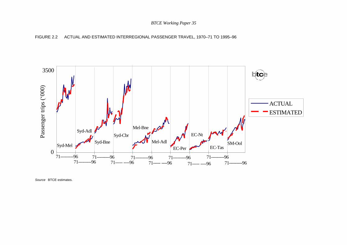
The model was estimated using cross–section and time series data between1970–71 and 1995–96 for the 10 interregional links. This basic equationaccounted for 85 per cent of the variation, with most of the residual variationbeing explained by some consistent differences between routes in levels oftravel (not growth rates). By assigning dummy variables to fine tune levels inthe corridors and to cater for special events (such as Expo in Brisbane (1988),the pilot strike (1990–91), etc.), the model explained about 97 percent of thevariance in total passenger travel on the links (figure 2.2).
Having derived a gravity model to explain growth in total passenger travel, thesecond step was to account for the long–term trends in modal share. Thisallowed prediction of the relative share of car traffic in the total transport market(which includes air, rail, coaches, and/or ferry) between pairs of interregionallinks. Logistic–substitution models were derived to measure the relative sharesof different transport modes over the period 1970–71 and 1995-96. The results
BTCE Working Paper 35
FIGURE 2.2 ACTUAL AND ESTIMATED INTERREGIONAL PASSENGER TRAVEL, 1970–71 TO 1995–96
ACTUAL
ESTIMATED
Syd-Mel SM-OolEC-Tas
EC-Nt
EC-Per
Mel-Adl
Mel-Bne
Syd-Cbr
Syd-Bne
Syd-Adl
71---------96 71---------9671---------96 71----- ----96
71---------9671----- ----96
71---------9671----- ----96
71---------9671---------96
3500
Pass
enge
r tr
ips
(‘00
0)
0
Source BTCE estimates.

BTCE Working Paper 35
obtained from the models showed that travel on long routes is increasinglydominated by air transport, while shorter route travel is becoming dominated bycars. The BTCE’s logistic–substitution modelling suggested the following ‘rulesof thumb’ (table 2.1) for translating growth in total travel between two regionsinto growth in car travel.
TABLE 2.1 ‘RULES OF THUMB’ USED TO TRANSLATE GROWTH IN TOTAL TRAVELINTO GROWTH IN CAR TRAVEL
Distance category ‘Rules of thumb’
Car growth multiplier(Applied to predicted
total growth)
Long routes (> 800 km) No growth in car travel 0.00
Medium routes (400–800 km) Car gains some of total growth 0.70
Short routes (200–400 km) Car winning mode share 1.25
Very short routes (< 200 km) Mostly car already 1.00
Source BTCE.
LOCAL CAR TRAFFIC
The growth in local car traffic was assumed to be proportional to ‘impliedvehicle kilometres travelled (VKT)’. ‘Implied VKT’ was measured as a product ofthe population of rural Statistical Local Areas (SLAs), cars per person at anational level, and national level non–urban VKT. The model is specified asfollows:
Rural local VKT
= Implied VKT
= (Rural SLAs Population x National - level Cars Per Person x
National - level Non - Urban VKT Per Car)
(2)
The rationale for using the ‘implied VKT’ approach in modelling rural localtravel relied upon two pieces of evidence. First, estimation conducted for urbanVKT found that traffic in the cities is closely approximated by this model.Secondly, subtracting from the 1995 Survey of Motor Vehicle Usage estimate ofnon–urban VKT, the interregional VKT (derived from tourism data), results in afigure for rural local VKT quite close to the figure for ‘implied VKT’.
THE FINAL TOTAL AADT FORECAST
The forecast of the final total AADT required forecasts of AADTs for bothcommercial vehicles and cars. In the absence of data or detailed forecasts,commercial vehicle AADT was assumed to grow at a rate of 3 per cent per

BTCE Working Paper 35
year. The forecast of car AADT was obtained by adding up the forecasts ofthrough car traffic as well as the rural local car traffic.
With respect to forecasting through car traffic, the growth in total travelbetween pairs of interregional links between 1996 and 2020 was based on theassumptions that:
• the product of the populations of the origin and destination interregional linksis multiplied by 0.5. Population growth assumptions on an SLA base weresupplied by the ABS (and averaged about 1.0 per cent per year nationally);
• there will be no change in real generalised costs of travel, and the growth inreal average weekly earnings will be one per cent per year. Hence thedenominator in equation (1) contributed 1.25 per cent per year to growth intotal travel demand.
Growth in total passenger demand was converted to growth in car passengerdemand by multiplying by the car growth multiplier matrix. The resultingforecast of car passenger movements was converted into a forecast origin–destination matrix of car trips using the assumption of 1.8 adults per car onlong–distance trips. The car travel matrix was then assigned to the roadnetwork (using the TRANSCAD computer program) in order to produceforecasts of through car traffic on highway sections.
For the forecasting of rural local traffic, the major assumptions associated withthe factors affecting rural local travel between 1996 and 2020 were as follows:
• ABS forecasts of growth of the population of rural SLAs (nationally about oneper cent per year but varying by SLA) were used;
• the national–level non–urban VKT per vehicle was assumed to remainconstant; and
• the national–level number of cars per person (cars plus light commercialvehicles) was assumed to grow at an average rate of 0.7 per cent per year.
Based on the assumptions adopted in the forecasting of through car traffic andrural local car traffic, the growth in the total light vehicle traffic therefore wasestimated to be in the order of 2 per cent per year nationally.
Figure 2.3A shows the forecast distribution of non–urban road sections on theNational Highway System in Western Australia by growth rate in AADT. Themedian growth forecast is about 2 percent growth as expected. Figure 2.3Bshows the historical distribution of road sections in Western Australia by growthrate in AADT (1989–90 to 1995–96). It is similar to but somewhat higher thanlevels predicted for the next two decades. It must be borne in mind, however,that growth in both population and vehicles per person will be markedly slowerover the next 20 years, and thus the forecast growth should indeed besomewhat lower than historical growth.

BTCE Working Paper 35
The final output of the forecast procedure was a file of predicted light andheavy vehicle traffic on each road section of the NHS. This was fed into theRIAM cost benefit model.
FIGURE 2.3A FORECAST TRAFFIC GROWTH ON WA NATIONAL HIGHWAY LINKS,1996–2020
m1
0
2
4
6
8
10
12
14
16
18
No
Lin
ks
0 1 2 3 4 5 6 7
Annual traffic growth (per cent)
Source BTCE.
FIGURE 2.3B HISTORICAL TRAFFIC GROWTH AT WA NATIONAL HIGHWAY COUNTSTATIONS, 1989–1996
m1 0 1 2 3 4 5 6 7 8 9 10 11 12 13
0
0.5
1
1.5
2
2.5
3
No
Sta
tio
ns
14
Annual traffic growth (per cent)
Source WA Main Roads.

BTCE Working Paper 35
CHAPTER 3 ROAD CAPACITY
The capacity of a road to carry traffic depends on characteristics such as thenumber of lanes, lane widths, shoulder widths, curvature and gradient.
Where the traffic volume is small in relation to road capacity, vehicles cantravel at their desired speed, free from interference from other road users. Astraffic volume rises, vehicles begin to slow each other down. With furtherincreases in traffic, congestion sets in. Investing in wider, straighter roadsreduces congestion on a road for any given traffic volume, yielding benefits interms of time, vehicle operating costs and accident cost savings.
However, the resulting benefits need to be compared to the costs of upgradingto test whether increasing road capacity is economically warranted.
METHODOLOGY AND ASSUMPTIONS
In assessing the capacity of non–urban roads, the RIAM model recognises theseries of discrete road standards shown in table 3.1. Each section of road inthe database is assigned the standard that best approximates its currentstandard. Depending on the terrain, generic project construction costs areassumed (table 3.2) for upgrading from each standard to the next. Theseproject costs include an allowance for upgrading of bridges and construction ofinterchanges. Expenditures required to replace existing bridges on the NHS arecovered separately in chapter 6.
For each segment of road, the RIAM model tests whether, given the traffic levelforecast, upgrading to higher standards is economically warranted. This is doneby comparing the benefits from upgrades with the costs of upgrading. Benefitsestimated are savings in vehicle operating costs, travel time, and accidentcosts. A large part of these benefits will be passed on to industries andconsumers. Additional maintenance costs to the road authority are added in asa negative benefit. Assumptions employed in estimating benefits are given inappendix I.

BTCE Working Paper 35
TABLE 3.1 ROAD STANDARDS INCORPORATED IN BTCE RIAM MODEL
Number oflanes
Lane width(m)
Sealedshoulder
width (m)a
Designspeed(kph)
AverageNRM over
timeb
2 lane narrow, unsealed shoulders 2 3.0 0 100 100
2 lane narrow, sealed shoulders 2 3.0 3.0 100 100
2 lane wide 2 3.5 2.6 100 90
2 lanes with 1.2 km overtakinglanes every 20 kms
2 3.5 2.6 100 90
2 lanes with 1.2 km overtakinglanes every 10 kms
2 3.5 2.6 100 90
2 lanes with 1.2 km overtakinglanes every 5 kms
2 3.5 2.6 100 90
4 lane divided 4 3.5 6.0 110 80
6 lane divided 6 3.5 6.0 110 70
8 lane divided 8 3.5 6.0 110 70
Notes a. Sealed shoulder widths are the sum of sealed widths for both shoulders (eg. for a 2 lane road, left and rightshoulders added together). Roads may also have unsealed shoulders but these are not specified because theyare assumed to contribute to increasing the capacity of the road.
b. NRM = National Association of Australian State Road Authorities (NAASRA) Roughness Measure. Roughnesslevels can be as low as 20 NRM for a new pavement and will deteriorate with age. Eventually the road will berehabilitated, returning it to the level for a new pavement. Higher standard roads are assumed to be rehabilitatedmore often and so have a lower average roughness over time.
Source BTCE.
TABLE 3.2 ASSUMED COST OF UPGRADING FROM ONE STANDARD TO THE NEXT
($’000 per kilometre)
Terrain
From standard To standard Flat Undulating Mountainous
2 lane narrow unsealedshoulders
2 lane narrow sealedshoulders
30 30 30
2 lane narrow, sealedshoulders
2 lane wide, sealedshoulders
200 200 200
2 lane wide 2 lanes with overtakinglanes every 20 kms
40 60 80
2 lanes with overtakinglanes every 20 kms
2 lanes with overtakinglanes every 10 kms
40 60 80
2 lanes with overtakinglanes every 10 kms
2 lanes with overtakinglanes every 5 kms
80 120 160
2 lanes with overtakinglanes every 5 kms
4 lane divided 2,900 4,300 5,800
4 lane divided 6 lane divided 4,300 6,400 8,600
6 lane divided 8 lane divided 4,300 6,400 8,600
Source BTCE based on information from various state and territory road authorities.

BTCE Working Paper 35
An allowance is made for new traffic generated as a result of improved roadconditions. An upgrade is deemed likely to be warranted if its economicallyoptimal implementation time occurs before the ‘snapshot’ dates used (1998,2005 and 2020). Use of an optimal timing criterion ensures that the presentvalue of net gains to Australia from road investment are maximised. If oneupgrade is found to be justified, the model also tests whether upgrades to stillhigher standards are warranted.
The discount rate used was 7 per cent, in line with Austroads practice. Choiceby the BTCE of a 7 per cent discount rate does not imply that it is the ‘correct’rate to use to assess the viability of a road investment. It was used to facilitateany comparisons with other road studies, and work done for the NationalPlanning Task Force (1994) by the BTCE.
The BTCE’s RIAM model incorporates the vehicle operating cost component ofthe World Bank’s Highway Design and Maintenance Standards Model (HDM–III) as revised for Australian conditions and updated by ARRB TransportResearch Ltd (Thoresen and Roper 1996, Roper and Thoresen 1997). TheBTCE has added a component that adjusts speed to take account ofcongestion for each level of hourly traffic volume throughout the year. Themodel also includes an algorithm to predict the effects of overtaking lanes onvehicle speeds.
Whether a length of road should be upgraded to a higher standard oneconomic grounds depends largely on the average annual daily traffic (AADT)level. The proportion of heavy vehicles is also quite influential. A truck createsmore congestion than a car and, because trucks have higher operating andtime costs than cars, benefits of road improvements are higher where there aregreater numbers of heavy vehicles. Terrain has a significant effect becauseupgrading costs are higher in rougher terrain, but so also are the benefits toroad users.
In order to confirm that the model is producing reasonable results, ‘thresholdAADTs’ were estimated under a range of heavy vehicle proportion and terrainscenarios. The thresholds are the minimum AADT level at which it justbecomes economic to upgrade from one standard to the next. These arepresented in table I.1, in Appendix I. As an example, a road in flat terrain with10 per cent of its AADT comprising heavy vehicles, would require at least anAADT of 1 981 vehicles per day to justify sealing the shoulders. Once the trafficvolume reached 12 085, duplication (upgrading from two lanes with overtakinglanes to four lane divided) would be warranted. The values in the table appearto be reasonable.

BTCE Working Paper 35
TABLE 3.3 EXPENDITURE NEEDS FOR CAPACITY EXPANSION BY STATE ANDTERRITORY: NATIONAL HIGHWAY SYSTEM
($ million)
State
Lengthanalysed
(km) Backlog (1998) 1999–2005 2006–2020 Total
ACT 17 4 – – 4
NSW 2,760 1,244 276 1,722 3,242
NT 2,620 – – – –
QLD 3,820 338 253 1,492 2,083
SA 2,379 31 72 264 366
TAS 299 62 35 151 248
VIC 1,145 235 10 550 796
WA 4,523 14 76 139 229
Overall 17,561 1,928 721 4,317 6,967
Source BTCE, based on data generously provided by state and territory road authorities.
RESULTS FOR THE NHS
Table 3.3 shows the results aggregated by States and Territories. The totalrequired expenditure for capacity upgrades of the type under considerationamounts to $7.0 billion over the 22 year forecast period. The backlogcomprises 28 per cent of the total. New South Wales requires the largestshare, accounting for 47 per cent of the total, followed by Queensland at 30 percent. The model did not find any upgrading to be warranted (at the strategiclevel) for the Northern Territory.
A more detailed breakdown by corridor is provided in table 3.4. The two maineast coast routes, Sydney–Brisbane (New England Highway) and Brisbane–Cairns (Bruce Highway) together account for more than half the forecastexpenditures. This accords with forecasts that the largest population growthsare likely to occur along the east coast.
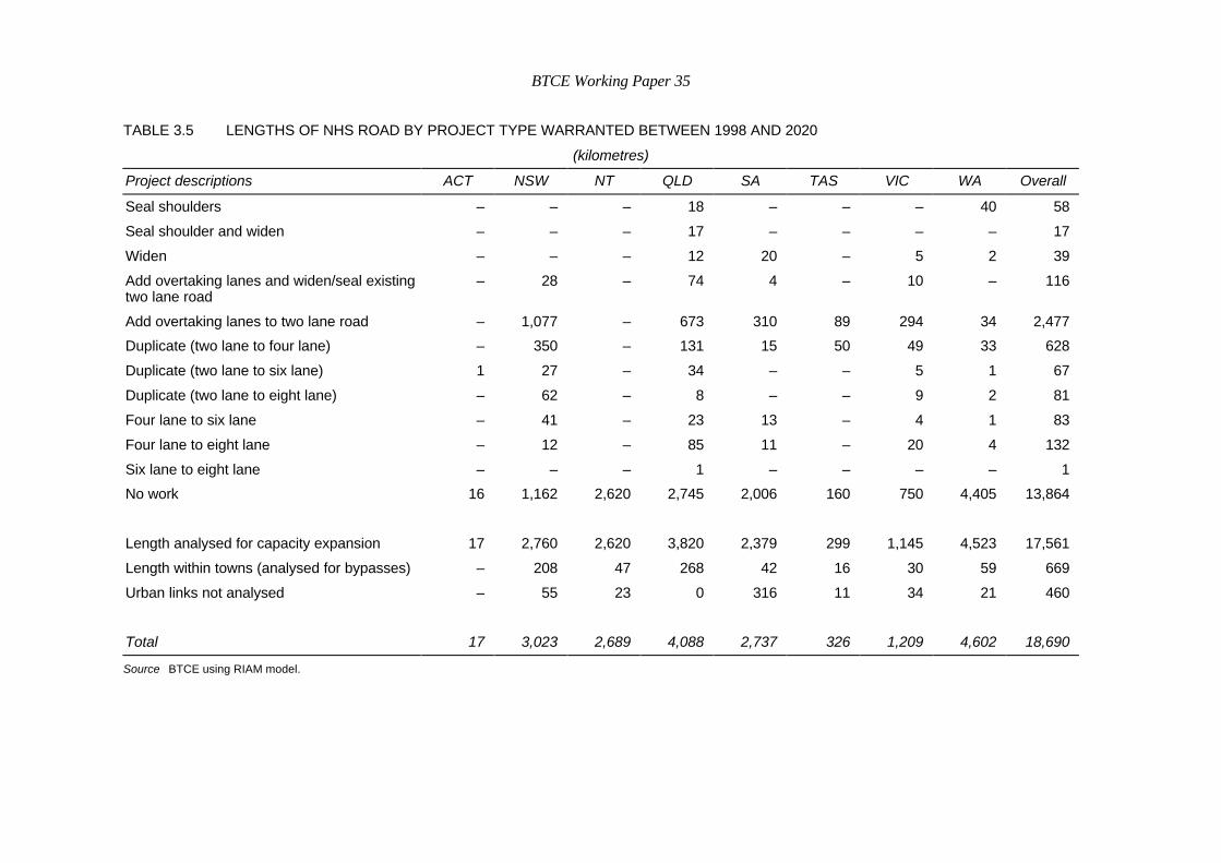
Tables 3.5 and 3.6 show how the forecasts are split up between different typesof upgrades by distance and cost. In terms of distance, addition of overtakinglanes predominates. They are a relatively inexpensive way to increase thecapacity of two lane roads. The main expenditures, however, are for highwayduplication because this is such a costly upgrading work.
A high proportion of the forecast expenditures occurs close to state capitals.

BTCE Working Paper 35
TABLE 3.4 EXPENDITURE NEEDS FOR CAPACITY EXPANSION BY CORRIDOR:NATIONAL HIGHWAY SYSTEM
($ million)
State Corridor
Lengthanalysed
(km)Backlog(1998) 1999–2005 2006–2020 Total
ACT Canberra Connections 17 4 – – 4
NSW Canberra Connections 103 23 2 18 44
NSW Melbourne to Brisbane 982 49 22 84 155
NSW Melbourne to Sydney 474 416 150 306 872
NSW Sydney to Adelaide 591 41 5 12 57
NSW Sydney to Brisbane 609 715 96 1,302 2,113
NT Adelaide to Darwin 1,717 – – – –
NT Brisbane to Darwin 434 – – – –
NT Perth to Darwin 469 – – – –
QLD Brisbane to Cairns 1,494 222 210 1,295 1,727
QLD Brisbane to Darwin 1,893 15 39 134 188
QLD Melbourne to Brisbane 218 1 0 2 3
QLD Sydney to Brisbane 215 100 4 60 164
SA Adelaide to Darwin 927 – – – –
SA Adelaide to Perth 954 15 8 23 47
SA Melbourne to Adelaide 277 5 61 187 252
SA Sydney to Adelaide 221 11 3 54 68
TAS Hobart to Burnie 299 62 35 151 248
VIC Melbourne to Adelaide 378 189 7 367 564
VIC Melbourne to Brisbane 250 45 3 184 232
VIC Melbourne to Sydney 284 – – – –
VIC Sydney to Adelaide 233 – – – –
WA Adelaide to Perth 1,391 12 24 111 147
WA Perth to Darwin 3,132 3 52 28 82
Overall 17,561 1,928 721 4,317 6,967
Source BTCE estimates using RIAM model.
Table 3.7 shows that 27 per cent of the total forecast expenditure for capacityexpansion occurs within 100 kilometres of Sydney, Melbourne, and Brisbaneand within 50 kilometres of the other capital cities.
BTCE Working Paper 35
TABLE 3.5 LENGTHS OF NHS ROAD BY PROJECT TYPE WARRANTED BETWEEN 1998 AND 2020
(kilometres)
Project descriptions ACT NSW NT QLD SA TAS VIC WA Overall
Seal shoulders – – – 18 – – – 40 58
Seal shoulder and widen – – – 17 – – – – 17
Widen – – – 12 20 – 5 2 39
Add overtaking lanes and widen/seal existingtwo lane road
– 28 – 74 4 – 10 – 116
Add overtaking lanes to two lane road – 1,077 – 673 310 89 294 34 2,477
Duplicate (two lane to four lane) – 350 – 131 15 50 49 33 628
Duplicate (two lane to six lane) 1 27 – 34 – – 5 1 67
Duplicate (two lane to eight lane) – 62 – 8 – – 9 2 81
Four lane to six lane – 41 – 23 13 – 4 1 83
Four lane to eight lane – 12 – 85 11 – 20 4 132
Six lane to eight lane – – – 1 – – – – 1
No work 16 1,162 2,620 2,745 2,006 160 750 4,405 13,864
Length analysed for capacity expansion 17 2,760 2,620 3,820 2,379 299 1,145 4,523 17,561
Length within towns (analysed for bypasses) – 208 47 268 42 16 30 59 669
Urban links not analysed – 55 23 0 316 11 34 21 460
Total 17 3,023 2,689 4,088 2,737 326 1,209 4,602 18,690
Source BTCE using RIAM model.

BTCE Working Paper 35
TABLE 3.6 COSTS OF NHS ROAD BY PROJECT TYPE WARRANTED BETWEEN 1998 AND 2020
($ million, 1997–98 prices)
Project descriptions ACT NSW NT QLD SA TAS VIC WA Overall
Seal shoulders – – – 1 – – – 1 2
Seal shoulder and widen – – – 4 – – – – 4
Widen – – – 3 4 – 1 1 8
Add overtaking lanes and widen/sealexisting two lane road
– 7 – 28 2 – 4 – 41
Add overtaking lanes to two lane road – 153 – 103 42 16 41 4 359
Duplicate (two lane to four lane) – 1,459 – 489 63 224 210 117 2,563
Duplicate (two lane to six lane) 4 286 – 332 – – 34 9 666
Duplicate (two lane to eight lane) – 1,010 – 122 – 8 153 36 1,328
Four lane to six lane – 193 – 101 96 – 15 5 411
Four lane to eight lane – 133 – 897 159 – 336 56 1,581
Six lane to eight lane – – – 4 – – – – 4
Total 4 3,242 – 2,083 366 248 795 229 6,967
Source BTCE using RIAM model.

BTCE Working Paper 35
TABLE 3.7 QUASIURBAN DEVELOPMENTa
(Percentage of expenditure needs for capacity expansion)
State Backlog (1998) 1999–2005 2006–2020 Total
ACT 100 n.a. n.a. 100
NSW 7 1 12 9
NT n.a. n.a. n.a. n.a.
QLD 31 42 41 40
SA 56 82 74 74
TAS 0 1 0 0
VIC 0 0 59 41
WA 100 99 97 98
Overall 10 34 33 27
Note a. Quasiurban development is defined as development occurring within 100 kilometres of Sydney, Melbourne andBrisbane, and within 50 kilometres of the other capital cities.
Source BTCE estimates using RIAM model.
QUALIFICATIONS TO ANALYSIS
Major realignment and flood mitigation projects
Future expenditures for major realignment and flood mitigation projects couldnot be estimated. To a certain extent, however, these expenditures are alreadyincluded, because higher construction costs are assumed for projects inrougher terrain and some bridge construction projects will improve immunityfrom flooding. Nevertheless, some underestimation of costs still occurs,although it is probably not very great in relation to the total.
Western Australia has informed the BTCE (David Rice, pers. comm.19 September 1997) that it has significant flood problems to overcome in theKimberley region, where road closures of one or two weeks per year still occur.
Provision by the States and Territories of detailed information such as floodfrequency and intensity, duration of traffic disruption, cost of repairs etc wouldpermit some assessment of potential mitigation projects. The BTCE would behappy to pursue such modelling enhancements in cooperation with the Statesand Territories.
Widening roads for road trains
Increasingly, double and triple road trains are being used to transport goodsbetween Australia’s western and northern states. State and Territory roadauthorities agree that road trains raise safety concerns on existing roads, which

BTCE Working Paper 35
were built for standard truck configurations. The preferred solution is to widenroads to around 8 or 9 metres seal width.
The BTCE’s modelling and analysis are based on economic criteria. To beconsistent with the BTCE approach, a cost–benefit analysis of widening roadsfor road trains would need to be undertaken. The cost–benefit analysis wouldtest whether the savings in accident costs as well as the other benefits arisingfrom increased road capacity, were sufficient to cover the additional capital andmaintenance costs. The BTCE has asked the road authorities concerned toprovide estimates of the cost of raising their sections of the NHS to thestandard they consider necessary to cater for road trains. Their estimates areset out in table 3.8. Western Australia and Queensland require the bulk ofupgrading work necessary for road trains. Western Australia has more roadlength requiring upgrading than other states. Queensland’s roads requirecomplete rebuilding, as opposed to widening, which is sufficient in other states.
TABLE 3.8 SUMMARY OF STATE AND TERRITORY ROAD TRAIN REQUIREMENTSa
Necessary upgrading work
StateMinimum standard for
road trains RebuildWidening &
seal shoulder
Approximatecost
($ million)
NorthernTerritory
8m seal – 1170km 31
New SouthWales
n.a. n.a.
Queensland 9m seal 632km – 316
South Australia 8m seal – 659km 98b
WesternAustralia
AADT<3000: 8m sealAADT>3000: 9m seal
2,318km61km
619
Note a. The estimates in the table have not been subjected to cost–benefit analysis by the BTCE.
b. Includes $60 million for rebuilding and widening the Sturt Highway.
Sources pers. com. Phil Cross, Department of Transport and Works, Northern Territory, 17 September 1997; pers. com.Viv Manwaring, Roads and Traffic Authority, New South Wales, 17 September 1997; pers. com. Eddie Peters,Queensland Department of Main Roads, 19 September 1997; pers. com. Bert Rowe, Department of Transport,South Australia, 11 September 1997; pers. com. David Rice, Main Roads, Western Australia, 17 September1997.
State and Territory estimates of the total cost of upgrading the NHS to takeroad trains are in the order of $1 billion. However, unqualified addition of thisestimate to the BTCE’s estimates of increased road capacity requirements islikely to involve some double counting, since RIAM’s $7.0 billion estimate forcapacity works includes some road widening. The Queensland costs includepavement reconstruction work which is already included in the BTCE’s

BTCE Working Paper 35
estimates of maintenance needs. Because the costs of widening for road trainshave not been subjected to an economic test, they have not been added to theBTCE’s totals. The economic viability of road upgrading depends to a largeextent on traffic levels. For example, in Western Australia most of the NHScarries low levels of traffic (half of the length of NHS road in Western Australiaassessed for capacity had AADT levels of less than 350 vehicles per day as at1998), so it is probable that much of the widening work suggested for roadtrains would not pass a cost–benefit test. However, the information in table 3.8is useful in that it provides an indication of the likely magnitude of the cost ofwidening roads for road trains.
SENSITIVITY TESTS
Sensitivity tests have been undertaken for varying forecast traffic levels, thediscount rate, construction costs, and the annual hourly volume distribution.The results of these tests are presented in table 3.9. The table shows thepercentage changes from the basecase presented above, for expenditure totalsfor each state and for the total of all states.
There is fair amount of variability between states. If a significant proportion of astate’s road system has traffic levels close to threshold levels for upgrading tohigher standards, small changes in assumptions can lead to large movementsacross thresholds and hence large effects on forecast expenditure needs. Theless the length of road being analysed in a state or territory, the morepronounced these effects can be, as seen by the Australian Capital Territoryresults. The tests show that for the Northern Territory, traffic levels fall wellshort of thresholds.
The expenditure forecasts are very sensitive to traffic level forecasts, but lessso for construction costs. Increasing construction costs lowers threshold AADTlevels, thus reducing the total distance upgraded but raises the requiredexpenditures for the remaining upgrades. In most cases, the latter effectpredominates. The change in expenditure levels from increasing the discount isnot very great considering the size of increase in the discount rate: from 7 to12 per cent.
Congestion along a road varies throughout the day, week and year. RIAMmodels congestion on the basis of hourly traffic volumes. The model needs toassume a distribution of these volumes across all the hours of the year. Twodistributions are employed, ‘rural’ and ‘quasiurban’. The quasiurban distributionis slightly flatter and is used for roads close to capital cities. The WesternAustralian annual hourly volume distribution is a composite of a number ofdistributions supplied to the BTCE by Main Roads WA. All three distributionsare presented in appendix I.

BTCE Working Paper 35
Two sensitivity tests were undertaken with respect to the hourly volumedistributions: one replacing only the rural distribution and one replacing boththe rural and quasiurban distributions. The Western Australian distribution isquite different in character from the rural and quasiurban distributions and canhave a marked effect on the results for individual states.
TABLE 3.9 SENSITIVITY TESTS FOR CAPACITY EXPANSION FORECASTS
Per cent change in results
Sensitivity Test ACT NSW
NT QLD SA TAS VIC WA Total
+20% AADT in 2020 290 58 0 82 86 61 118 59 66
-20% AADT in 2020 0 -34 0 -15 -63 -51 -46 -21 -40
12% discount ratea 0 -23 0 20 -23 -47 -16 -10 -22
+20% construction costs 20 18 0 55 15 19 9 12 15
-20% construction costs 160 -7 0 29 -1 -17 1 -19 -7
WA hourly volumedistribution: rural only
0 -3 0 27 -1 -29 -10 0 -7
WA hourly volumedistribution: rural andquasiurban
225 -1 0 39 30 -29 -6 21 0
Note a. 7 per cent discount rate used as default in RIAM.
Source BTCE estimates using RIAM model.

BTCE Working Paper 35
CHAPTER 4 TOWN BYPASSES
Traffic passing through a town experiences delays itself, while generatingcongestion for local traffic within the town. Construction of a town bypasstherefore benefits both through–traffic and local traffic. In much the samemanner as for capacity expansion projects, the RIAM model is able to testwhether or not construction of town bypasses is warranted.
METHODOLOGY AND ASSUMPTIONS
For each town bypass assessed by RIAM, the length of the bypass has beentaken as the total distance of road sections in and around the town with legalspeed limits of less than 100 kilometres per hour. The construction cost hasbeen estimated from the generic costs per kilometre presented in table 4.1. TheQueensland Department of Main Roads supplied their own estimates of lengthsand costs for the bypasses assessed on national highways in Queensland.These lengths and costs were used in place of the RIAM estimates.
TABLE 4.1 ASSUMED COSTS FOR TOWN BYPASS CONSTRUCTION
($’000 per kilometre)
Terrain
Flat Undulating Mountainous
Two lane bypass 2,300 2,900 5,300
Four lane bypass 4,100 5,300 9,300
Source BTCE estimates.
The model distinguishes between through–traffic and local traffic. For cars,through–traffic is estimated from the interregional traffic flow generated duringthe course of developing the total AADT forecasts. For trucks, it is estimatedfrom the traffic counts in the database. Not all of the through–traffic would use abypass. It is assumed that a certain proportion will continue to use the townroad despite construction of the bypass.
BTCE Working Paper 35
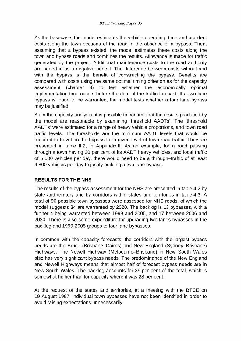
As the basecase, the model estimates the vehicle operating, time and accidentcosts along the town sections of the road in the absence of a bypass. Then,assuming that a bypass existed, the model estimates these costs along thetown and bypass roads and combines the results. Allowance is made for trafficgenerated by the project. Additional maintenance costs to the road authorityare added in as a negative benefit. The difference between costs without andwith the bypass is the benefit of constructing the bypass. Benefits arecompared with costs using the same optimal timing criterion as for the capacityassessment (chapter 3) to test whether the economically optimalimplementation time occurs before the date of the traffic forecast. If a two lanebypass is found to be warranted, the model tests whether a four lane bypassmay be justified.
As in the capacity analysis, it is possible to confirm that the results produced bythe model are reasonable by examining ‘threshold AADTs’. The ‘thresholdAADTs’ were estimated for a range of heavy vehicle proportions, and town roadtraffic levels. The thresholds are the minimum AADT levels that would berequired to travel on the bypass for a given level of town road traffic. They arepresented in table II.2, in Appendix II. As an example, for a road passingthrough a town having 20 per cent of its AADT heavy vehicles, and local trafficof 5 500 vehicles per day, there would need to be a through–traffic of at least4 800 vehicles per day to justify building a two lane bypass.
RESULTS FOR THE NHS
The results of the bypass assessment for the NHS are presented in table 4.2 bystate and territory and by corridors within states and territories in table 4.3. Atotal of 90 possible town bypasses were assessed for NHS roads, of which themodel suggests 34 are warranted by 2020. The backlog is 13 bypasses, with afurther 4 being warranted between 1999 and 2005, and 17 between 2006 and2020. There is also some expenditure for upgrading two lanes bypasses in thebacklog and 1999-2005 groups to four lane bypasses.
In common with the capacity forecasts, the corridors with the largest bypassneeds are the Bruce (Brisbane–Cairns) and New England (Sydney–Brisbane)Highways. The Newell Highway (Melbourne–Brisbane) in New South Walesalso has very significant bypass needs. The predominance of the New Englandand Newell Highways means that almost half of forecast bypass needs are inNew South Wales. The backlog accounts for 39 per cent of the total, which issomewhat higher than for capacity where it was 28 per cent.
At the request of the states and territories, at a meeting with the BTCE on19 August 1997, individual town bypasses have not been identified in order toavoid raising expectations unnecessarily.

BTCE Working Paper 35
TABLE 4.2 EXPENDITURE NEEDS FOR TOWN BYPASSES BY STATE ANDTERRITORY: NATIONAL HIGHWAY SYSTEM
($ million)
State
Number ofbypassesassessed
Number ofbypasseswarranted Backlog 1999–2005 2006–2020 Total
NSW 22 14 412 117 171 700
NT 5 – – – – –
QLD 24 10 195 288 190 673
SA 11 2 – – 27 27
TAS 4 3 – – 45 45
VIC 6 5 – – 96 96
WA 18 – – – – –
Overall 90 34 607 405 529 1,541
Source BTCE using RIAM model.
TABLE 4.3 EXPENDITURE NEEDS FOR TOWN BYPASSES BY CORRIDOR: NATIONALHIGHWAY SYSTEM
($ million)
State Corridor
Number ofbypassesassessed
Number ofbypasseswarranted Backlog
1999–2005
2006–2020 Total
NSW Melbourne to Brisbane 9 4 92 117 21 229
NSW Melbourne to Sydney 1 1 145 – – 145
NSW Sydney to Adelaide 3 1 40 – – 40
NSW Sydney to Brisbane 9 8 136 – 150 286
NT Adelaide to Darwin 5 0 – – – –
QLD Brisbane to Cairns 8 7 55 167 171 393
QLD Brisbane to Darwin 14 2 140 110 11 261
QLD Sydney to Brisbane 2 1 – 11 9 20
SA Adelaide to Darwin 1 0 – – – –
SA Adelaide to Perth 3 0 – – – –
SA Melbourne to Adelaide 3 0 – – – –
SA Sydney to Adelaide 4 2 – – 27 27
TAS Hobart to Burnie 4 3 – – 45 45
VIC Melbourne to Adelaide 5 4 – – 90 90
VIC Melbourne to Brisbane 1 1 – – 7 7
WA Adelaide to Perth 8 0 – – – –
WA Perth to Darwin 10 0 – – – –
Overall 90 34 607 405 529 1,541
Source BTCE using RIAM model.

BTCE Working Paper 35
SENSITIVITY TESTS
The same sensitivity tests have been undertaken as for the capacity analysis.The results are presented in table 4.4. As with capacity, the bypass expenditureneeds forecasts are very sensitive to the demand forecasts, but less so for thediscount rate and construction costs. The South Australian results areparticularly sensitive because of the low basecase, for which only two bypassesare warranted.
TABLE 4.4 SENSITIVITY TESTS
Percentage change in expenditure needs for town bypasses
Sensitivity Test ACT NSW
NT QLD SA TAS VIC WA Total
+20% AADT in 2020 na 14 0 15 317 48 17 0 12
-20% AADT in 2020 na -47 0 -7 -100 -100 -56 0 -67
12% discount rate na 0 0 -12 -100 -53 -35 0 -20
+20% construction costs na 20 0 13 -100 -28 5 0 0
-20% construction costs na -20 0 -6 1 -20 -7 0 -28
WA hourly volumedistribution: rural only
na 0 0 0 -100 -53 -20 0 -18
WA hourly volumedistribution: rural andquasimodal
na 0 0 0 -100 -53 -20 0 -18
Note na not applicable because no bypasses were assessed for the ACT.
Source BTCE using RIAM model.
BTCE Working Paper 35
CHAPTER 5 MAINTENANCE
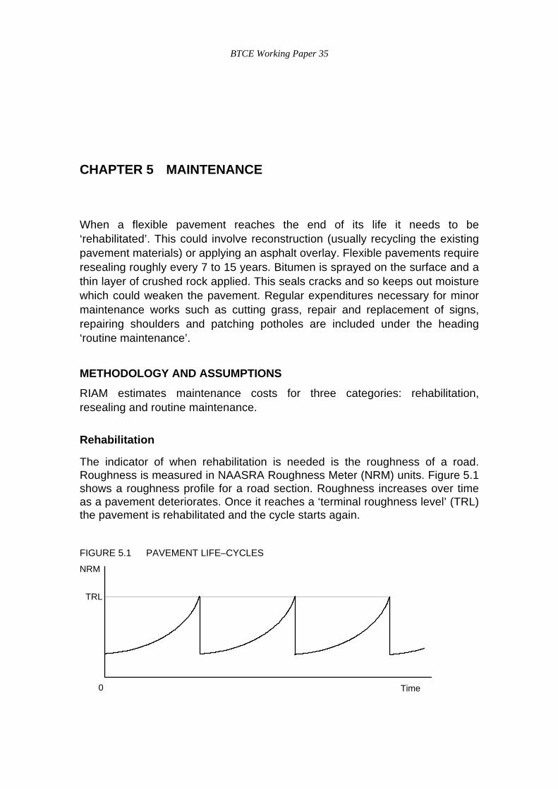
When a flexible pavement reaches the end of its life it needs to be‘rehabilitated’. This could involve reconstruction (usually recycling the existingpavement materials) or applying an asphalt overlay. Flexible pavements requireresealing roughly every 7 to 15 years. Bitumen is sprayed on the surface and athin layer of crushed rock applied. This seals cracks and so keeps out moisturewhich could weaken the pavement. Regular expenditures necessary for minormaintenance works such as cutting grass, repair and replacement of signs,repairing shoulders and patching potholes are included under the heading‘routine maintenance’.
METHODOLOGY AND ASSUMPTIONS
RIAM estimates maintenance costs for three categories: rehabilitation,resealing and routine maintenance.
Rehabilitation
The indicator of when rehabilitation is needed is the roughness of a road.Roughness is measured in NAASRA Roughness Meter (NRM) units. Figure 5.1shows a roughness profile for a road section. Roughness increases over timeas a pavement deteriorates. Once it reaches a ‘terminal roughness level’ (TRL)the pavement is rehabilitated and the cycle starts again.
FIGURE 5.1 PAVEMENT LIFE–CYCLES
NRM
Time0
TRL

BTCE Working Paper 35
To estimate how roughness changes over time, RIAM employs an algorithmdeveloped by ARRB Transport Research Ltd (Martin, T.C. 1996). The rate ofpavement deterioration in the ARRB algorithm depends on pavement strength,pavement age, the standard of maintenance (reseals and patching), weatherand the amount of truck traffic (cars do negligible damage to pavements).
For each section of road, the model fits a deterioration curve to the roughnesslevel recorded in the database in the particular year it was measured. Theassumed starting level for a new or rehabilitated pavement is 50 NRM.Because no information on pavement strength is available, the model estimatesthis from heavy vehicle traffic, under the assumption that pavements metAustroads design standards when built. (The assumed Austroads designstandards are based on traffic levels at the estimated rehabilitation time in thepast). Growth rates are expolated backwards in time to obtain the estimate ofpast design traffic. Weather is taken into account using the ‘ThornthwaiteIndex’. Values of this index were assigned to each section of road in thedatabase using information from a map in Aitchison and Richards (1965).
The model estimates the optimal times to undertake rehabilitations, minimisingthe discounted present value of combined road authority and road users’ costs.In determining the optimal rehabilitation times, the model is constrained so that,if the model has not found an optimum TRL below 160 NRM, rehabilitationautomatically occurs once the pavement reaches 160 NRM. The constraint hasbeen imposed because of advice that once roughness exceeds 160 NRM, thedeterioration rate accelerates and the pavement will soon break up (pers.comm. Jon Roberts, ARRB Transport Research Ltd, 11 September 1997).Where a rehabilitation is found to be warranted within the forecast period, thecost is added to the total.
Forecast rehabilitation costs depend principally on traffic levels (higher vehiclenumbers justify lower TRLs), climate (wetter climate leads to higherdeterioration rates), and current roughness. If a pavement has a low roughnesslevel, which indicates that it is relatively new, the pavement may not requirerehabilitation before 2020, particularly if the traffic level is low and the climatedry. The model found large numbers of sections of road falling into thiscategory.
Resealing
If a rehabilitation is predicted to occur within a forecast period, the model inturn predicts when reseals could occur. Once a pavement has beenrehabilitated, there will be no need for a reseal for some years. It would also bewasteful to reseal within several years prior to a rehabilitation. Where there are

BTCE Working Paper 35
no rehabilitations within the forecast period, the model assumes that resealsoccur every 10 years and allocates one tenth of the resealing cost to eachyear.
Routine maintenance
Routine maintenance is simply estimated on the basis of an amount per squaremetre per annum. Routine maintenance includes cutting grass, repair andreplacement of signs, filling potholes, and so on.
Cost assumptions
For all three types of maintenance, generic costs per square metre of pavementare assumed for each standard of road established for the capacity analysis.Unsealed shoulders are costed at different rates from the sealed road surface.Higher road capacity standards are associated with higher rehabilitation costsper square metre owing to greater traffic levels. Table 5.1 shows the costassumptions used by the BTCE.1
In order to test the model, optimal TRLs were obtained for the road standardsrecognised by RIAM over large range of AADT levels. These are presented ascharts in appendix II. For example, assuming 6 per cent rigid trucks and 18 percent articulated trucks (the averages for the NHS), two lane roads with AADTlevels below 1000 vehicles per day would be rehabilitated when they reached160 NRM, the maximum allowed by the model. At 2000 vehicles per day, theTRL falls to around 135 NRM. For two lane roads having 10 000 vehicles perday, the TRL is around 95 NRM. For four lane roads with 10 000 vehicles perday, the TRL is 128 NRM. Higher traffic levels lead to lower TRLs because thegreater the number of vehicles, the greater the benefits of smootherpavements. Higher rehabilitation costs will lead to higher TRLs because of thegreater cost to road authorities of providing smoother pavements. This is thereason for the higher TRL on a four lane road having the same AADT as twolane road.
1 Higher cost assumptions were employed for the ACT at the request of the ACT Department of Urban Services. It
argued that greater costs are incurred because of lack of economies of scale. The effect on the total forecasts isminuscule because the ACT only accounts for 17 kilometres of the NHS.

BTCE Working Paper 35
TABLE 5.1 COSTS ASSUMED FOR MAINTENANCE ASSESSMENT
($ per square metre of pavement area)
Rehabilitation Reseals Routine maintenance
Standard SealedUnsealedshoulder
Bitumensurface Asphalt Sealed
Unsealedshoulder
2 lane narrow, unsealedshoulders
30.00 20.00 2.50 12.50 1.00 1.25
2 lane narrow, sealedshoulders
30.00 20.00 2.50 12.50 1.00 1.25
2 lane wide (includingstandards where there areovertaking lanes)
30.00 20.00 2.50 12.50 1.00 1.25
4 lane divided 60.00 20.00 2.50 12.50 1.00 1.25
6 lane divided 60.00 20.00 2.50 12.50 1.00 1.25
8 lane divided 60.00 20.00 2.50 12.50 1.00 1.25
Note Reseals are assumed to occur every 10 years except when a rehabilitation occurs.
Source BTCE estimates, based on advice by State and Territory road authorities.
RESULTS FOR THE NHS
Forecast expenditure needs are shown by state and territory in table 5.2 and bycorridor in table 5.3. No backlog has been assumed for resealing and routinemaintenance as these expenditures occur with much greater frequency than forrehabilitation. Resealing and routine maintenance costs are roughlyproportional to the length of road analysed (width is also a factor).
There is very little backlog for rehabilitation except for the Brisbane-Darwincorridor in Queensland, but even then it is small. The implication is that thereare significant lengths of road with roughness levels currently aboveeconomical terminal roughness levels. For total rehabilitation costs, the majorcosts occur along the main east coast corridors where traffic levels are higherand deterioration rates are higher because of the wetter climate.
On an annual basis, the resealing and routine maintenance costs are similarfrom year to year. However, rehabilitation costs per year are considerablyhigher for all states and territories during the 2006–2020 period compared withthe 1999–2005 period plus the backlog. This suggests that pavements aregenerally in good condition at present, but that later in the forecast period, asignificant amount of pavement will need rehabilitating. Growth in trafficvolumes would also be a contributing factor to this unevenness in annualrehabilitation needs.

BTCE Working Paper 35
QUALIFICATIONS TO ANALYSIS
RIAM allows for only one kind of treatment (rehabilitation) which could meaneither a reconstruction or a thick overlay. There is a range of possiblemaintenance strategies involving thinner overlays which are cheaper, but lesseffective than a thicker overlay. Thinner overlay options have not beenconsidered because, where a number of alternative treatments are available,determining the optimum treatment and timing vastly increases the complexityof the optimisation problem. The results would also be very sensitive to theassumed costs of the various treatments. The purpose of strategic models suchas RIAM is primarily to draw attention to the need for closer investigation, whileproviding an approximate estimate of costs.
Concrete pavements have not had any maintenance costs attributed to them inthe RIAM model. They have much longer lives than flexible pavements, but,because they are a relatively recent phenomenon, there is great uncertaintyabout just how they will last. Routine maintenance costs for concretepavements are quite small, so no allowance has been made for this.
The forecasting of future capacity upgrading and town bypass needs has beencarried out separately from the forecasting of future maintenance needs.Maintenance costs of additional road pavement created over the coming22 years to increase capacity have not been included. Being new, theadditional pavements are unlikely to require rehabilitation during the forecastperiod. There will still be a need for routine maintenance and, in some cases, areseal. However, these additional costs will be minor in relation to the total.
In practice, a rehabilitation and upgrading to a higher standard would often beundertaken at the same time. A model that allowed for combined upgrading andrehabilitations would require a much more complex algorithm than currentlyused for RIAM. The effect on results is considered too small to justify thenecessary resources.
SENSITIVITY TESTS
Sensitivity tests have been undertaken, as for the capacity analysis, with theaddition of variations in the rate of change in roughness and the maximum TRL.The results are presented in table 5.4. They have been presented forrehabilitation costs only. Changes in the costs will affect resealing and routinemaintenance costs proportionately but changes in the other variables in thetable will have no effect whatsoever.
Rehabilitation costs are quite sensitive to the deterioration rate. Increasingrehabilitation costs can cause forecast expenditure needs to change in eitherdirection. Higher rehabilitation costs per square metre of pavement lead to

BTCE Working Paper 35
TABLE 5.2 EXPENDITURE NEEDS FOR MAINTENANCE BY STATE AND TERRITORY: NATIONAL HIGHWAY SYSTEM
($ million, 1997–98 prices)
RehabilitationResealing and routine
maintenancea All maintenance
StateLength of roadanalysed (km)
Backlog(1998)
1999–2005
2006–2020 Total
1999–2005
2006–2020 Total
Backlog(1998)
1999–2005
2006–2020 Total
ACT 17 0 1 10 11 3 5 8 0 4 15 19NSW 2,968 6 86 902 994 202 416 618 6 288 1,318 1,612NT 2,666 1 2 117 120 195 435 630 1 197 551 750QLD 4088 31 93 818 942 364 791 1155 31 457 1,609 2,097SA 2,421 0 3 93 96 226 525 751 0 229 618 847TAS 316 0 1 127 128 38 74 111 0 39 201 239VIC 1,177 6 26 385 418 127 297 425 6 153 683 842WA 4,581 3 11 105 120 394 858 1,252 3 405 963 1,372Overall 18233 49 224 2,556 2,829 1,548 3,401 4,949 49 1,772 5,957 7,777
Notes a. No backlog has been assumed for resealing and routine maintenance as these expenses are incurred with greater frequency than rehabilitations.
Source BTCE using RIAM model.

BTCE Working Paper 35
TABLE 5.3 EXPENDITURE NEEDS FOR MAINTENANCE BY CORRIDOR: NATIONAL HIGHWAY SYSTEM($ million, 1996–1997 prices)
Length ofroad Rehabilitation
Resealing and routinemaintenancea All maintenance
State Corridoranalysed
(km) Backlog1999–2005
2006–2020 Total
1999–2005
2006–2020 Total Backlog
1999–2005
2006–2020 Total
ACT Canberra Connections 17 0 1 10 11 3 5 8 0 4 15 19NSW Canberra Connections 103 0 2 59 60 10 20 29 0 11 78 90NSW Melbourne to Brisbane 1,059 3 53 169 225 61 122 183 3 114 291 408NSW Melbourne to Sydney 510 0 4 326 330 47 104 151 0 51 430 481NSW Sydney to Adelaide 609 3 4 118 125 37 70 107 3 40 189 232NSW Sydney to Brisbane 687 0 23 231 254 48 99 147 0 71 330 401NT Adelaide to Darwin 1,763 0 0 97 98 132 293 425 0 132 390 522NT Brisbane to Darwin 434 0 0 5 5 34 72 106 0 34 78 111NT Perth to Darwin 469 1 2 14 17 30 69 99 1 32 83 117QLD Brisbane to Cairns 1680 7 47 551 606 166 350 516 7 213 902 1122QLD Brisbane to Darwin 1950 18 30 168 216 158 350 508 18 188 518 725QLD Melbourne to Brisbane 223 2 4 32 17 38 55 2 21 70 93QLD Sydney to Brisbane
(inland route)234 4 12 66 81 23 52 75 4 35 118 157
SA Adelaide to Darwin 930 0 0 3 3 86 185 271 0 86 188 273SA Adelaide to Perth 965 0 0 16 16 88 193 281 0 88 209 297SA Melbourne to Adelaide 286 0 0 44 44 32 99 131 0 32 144 175SA Sydney to Adelaide 240 0 3 30 33 20 48 68 0 23 78 101TAS Hobart to Burnie 316 0 1 127 128 38 74 111 0 39 201 239VIC Melbourne to Adelaide 408 2 13 142 157 44 95 139 2 57 238 296VIC Melbourne to Brisbane 252 4 10 53 66 18 42 60 4 28 94 126VIC Melbourne to Sydney 284 0 1 164 165 49 125 174 0 50 290 339VIC Sydney to Adelaide 233 1 3 26 29 16 35 51 1 19 61 80WA Adelaide to Perth 1,421 2 7 68 77 117 259 376 2 124 327 453WA Perth to Darwin 3,160 1 4 37 43 277 599 876 1 281 636 919Overall 18,233 49 224 2,556 2,829 1,548 3,401 4,949 49 1,772 5,957 7,777Notes a. No backlog has been assumed for resealing and routine maintenance as these expenses are incurred with greater frequency than rehabilitations.
Source BTCE using RIAM model.

BTCE Working Paper 35
higher economically optimal TRLs which pushes rehabilitation times into thefuture. When rehabilitation times shift beyond 2020, the forecasts fall. Forsome states, such as South Australia, this effect outweighs higher unitrehabilitation costs.
The final sensitivity test shown in the table involves reducing the maximumroughness constraint from 160 NRM to 130 NRM. According to RIAM, there isno economic warrant for this, but it might be advocated for social or equityreasons. This has a large effect on the Northern Territory, Western Australiaand South Australia where low traffic levels lead to high economically optimalTRLs.
TABLE 5.4 SENSITIVITY TESTS: REHABILITATION COSTS
Per cent change in results
Sensitivity Test ACT NSW
NT QLD SA TAS VIC WA Total
+20% AADT in 2020 5 3 0 8 26 8 31 13 10
-20% AADT in 2020 -14 -9 -4 -12 -21 -11 -25 -20 -13
12% discount rate 0 -10 -3 -16 -28 -16 -31 -30 -17
+20% deterioration rate 10 8 77 263 86 15 52 42 106
-20% deterioration rate -16 -22 -74 -23 -45 -19 -39 -34 -28
+20% rehabilitation costs 3 16 16 8 -4 7 0 0 9
-20% rehabilitation costs -12 -17 -19 -11 16 -12 7 -6 -10
WA hourly volumedistribution
0 0 0 0 2 0 0 1 0
TRL constrained tomaximum of 130 NRM
0 0 299 14 65 3 1 93 24
Source BTCE using RIAM model.

BTCE Working Paper 35
CHAPTER 6 INCREASED VEHICLE WEIGHTS AND BRIDGEREPLACEMENT
Bridges are relatively more expensive to construct than road pavements, andare therefore designed for a longer service life. Failure of a bridge also hasmore severe transport consequences than a pavement failure, illustratedspectacularly by the loss of three spans of the Tasman Bridge in Hobartbecause of a ship collision.
The range of ages and strengths in Australia’s bridges reflects their longerservice life as well as the increase over time in the mass and number of heavyvehicles. For example, some bridges presently in service on national highwayswere designed and constructed over 50 years ago for loads half of thosecarried today. It is the design limits of these older bridges that limits potentialproductivity gains from increasing current limits on the weight of heavyvehicles.
The BTCE therefore commissioned Dr Rob Heywood (Queensland University ofTechnology) and Bob Pearson (Pearsons Transport Resource Centre P/L) toanalyse the adequacy of bridges on the NHS and other primary roads,including the costs of replacement if current mass limits on heavy vehicles wereincreased in the future. Their report is reproduced with minor editing atappendix IV.
BRIDGES ON THE NATIONAL HIGHWAY SYSTEM
The consultants analysed bridges on both the NHS and on a number of otherprimary roads (listed in table 2.1, appendix IV), but only the results for the NHSare reported in this chapter. The major source of data used was an earliersurvey of bridges as part of the National Road Transport Commission’s (NRTC)Mass Limits Review in 1996. The data collected by the NRTC is in aggregatedform and does not permit the identification of specific bridges.
There are about 1 976 bridges on the NHS network, of varying types, ages andspans. The superstructure material is predominantly concrete, almost 20 percent is steel, and there are still some timber bridges.

BTCE Working Paper 35
Design standard was used by the consultants as a surrogate for age as well asthe fundamental indicator of bridge strength. Three design load groupings wereconsidered, each designated by a design code:
• bridges built since 1976, referred to as T44, forming about 43 per cent ofbridges on the NHS;
• MS18 denotes bridges built between 1948 and 1976. Bridges of this designgrouping form about 46 per cent of NHS bridges; and
• the 11 per cent of pre–MS18 bridges which were built before 1948.
The Northern Territory has the highest proportion of bridges built to T44standard, but also the highest percentage of pre–1948 bridges. Victoria andTasmania have the lowest proportion of modern bridges. South Australia hasthe lowest proportion of pre–1948 bridges.
ANALYSIS
Bridges were assessed for their capacity to withstand loads under threescenarios of possible mass limits in the future for articulated vehicles (table 3.1,appendix IV provides detail):
• Scenario 1: gross mass increased from current level of 42.5 tonnes to45.5 tonnes, with no further increases;
• Scenario 2: gross mass increased to 45.5 tonnes in 1997, further increasedto 52 tonnes in 2010, with no further increases; and
• Scenario 3: as for scenario 2, but with a further increase to 58 tonnes in2020.
The model used by the consultants estimates bending of bridges under variousvehicle weights, and compares them to design standards for the bridge typeunder consideration. The model applies engineering judgement about theremaining life of a bridge, taking account of worst case truck loadings, ageing,traffic growth, environmental effects and the observed better than expectedperformance of bridges compared with the original design calculations. Abridge is deemed to need replacing once the risk of failure reaches anunacceptable level.
Replacement costs were estimated from the deck area of the existing bridgeusing a generic cost per square metre. It was assumed that replacementbridges are of concrete or steel at the T44 standard. There was no allowancemade for the additional costs of constructing wider, longer bridges withimproved alignments. These costs were allowed for in the capacity analysisthrough use of higher generic costs per kilometre than would be required forconstruction in the absence of bridges and interchanges.

BTCE Working Paper 35
Strengthening of bridges was not considered as an option. Hence the costspresented below are likely to be overestimates. Overestimation may have alsooccurred where bridges have been replaced or strengthened since thecollection of the data set used.
RESULTS
Costs of bridge replacement were estimated for four time periods: now (the1998 backlog), 1998–2005, 2006–2020, and 2021–2030. Estimates for theNHS are presented in table 6.1
The analysis shows that an immediate expenditure of $24 million is needed onthe NHS. Victorian bridges would require attention much earlier than those inother states. However, substantial expenditure would be required inQueensland and New South Wales in the early part of next century.2
The bridges on the NHS are generally in good condition, with almost halfhaving been built in the last 20 years. It should be borne in mind that theforecast bridge replacement costs for the NHS are not representative of thewider population of Australian bridges. The results obtained cannot thereforebe extrapolated to Australia as a whole.
2 It is not possible to make comparisons with the NRTC Mass Limits Review (National Road Transport Commission,
1996). The estimates above are costs of bridge replacement in 1996-97 dollars, whereas the Mass Limits Reviewcosts were estimates of the cost of bringing forward reconstruction, and it did not consider the cost of replacingbridges already considered deficient under existing mass limits.

BTCE Working Paper 35
TABLE 6.1 COSTS TO REPLACE BRIDGES UNDER DIFFERENT LOADING SCENARIOS ON THE NATIONAL HIGHWAY SYSTEM
($million, 1997–98 prices)
Scenario 1 Scenario 2 Scenario 3
Corridor now1998–2005
2006–2020
2021–2030 now
1998–2005
2006–2020
2021–2030 now
1998–2005
2006–2020
2021–2030
Sydney–Melbourne 4.3 5.9 10.7 8.5 4.3 5.9 26.2 13.7 4.3 5.9 26.2 56.0
Canberra connections 0.0 0.0 0.2 0.8 0.0 0.0 1.2 0.2 0.0 0.0 1.2 3.7
Sydney–Brisbane (New England Hwy) 0.2 0.1 2.2 8.1 0.2 0.1 17.1 4.2 0.2 0.1 17.1 41.8
Sydney–Adelaide (Sturt Hwy) 0.1 0.2 4.8 5.3 0.1 0.2 12.4 3.8 0.1 0.2 12.4 38.8
Melbourne–Adelaide 1.3 1.9 6.6 4.4 1.3 1.9 14.1 6.4 1.3 1.9 14.1 37.3
Melbourne–Brisbane (Newell Hwy) 1.2 1.4 3.7 6.6 1.2 1.4 17.4 6.2 1.2 1.4 17.4 37.6
Brisbane–Cairns 1.2 0.8 2.8 10.0 1.2 0.8 47.3 15.5 1.2 0.8 47.3 66.1
Adelaide–Perth 0.1 0.2 0.8 0.7 0.1 0.2 3.2 1.2 0.1 0.2 3.2 5.6
Adelaide–Darwin 2.8 1.7 0.6 0.6 2.8 1.7 7.3 0.5 2.8 1.7 7.3 4.8
Perth–Darwin 1.2 1.2 1.3 1.1 1.2 1.2 12.8 4.5 1.2 1.2 12.8 9.7
Brisbane–Darwin 0.9 0.5 0.3 1.2 0.9 0.5 7.0 1.8 0.9 0.5 7.0 7.7
Hobart–Burnie 10.6 1.1 0.9 0 10.6 1.1 5.5 1.2 10.6 1.1 5.5 12.1
Total 23.9 15.0 34.9 47.3 23.9 15.0 171.5 59.2 23.9 15.0 171.5 321.2
Source BTCE, see appendix IV.

BTCE Working Paper 35
CHAPTER 7 AGGREGATED RESULTS
Tables 7.1 and 7.2 show the aggregated results for the four types ofexpenditure considered for the NHS and for other roads considered to be ofmajor significance by the state and territory road authorities. Expenditure towiden roads to allow for road trains has been excluded.
Bridge replacement costs have been included, assuming the highest costvehicle mass limits scenario. Although an increase in mass limits to only45.5 tonnes is currently under discussion, it is highly likely that any bridges thatare replaced would be designed to far more than for an additional 3 tonne load.This is primarily because the marginal cost of building a bridge to a higherstandard is fairly low.
The total expenditure for the NHS for the 22 year forecast period is almost$17 billion. This is higher than the 1995–2015 forecast of $12.9 billiondeveloped by the BTCE for the National Transport Planning Taskforce. Thebacklog comprises 15.5 per cent of the total. Counting town bypassconstruction as a type of capacity expansion and bridge replacement as a typeof maintenance, there is roughly a 50:50 split between forecast capacityexpansion and maintenance expenditures.
New South Wales and Queensland have the largest expenditure needs.Together they account for two–thirds of the total. For these two states, forecastcapacity expenditure exceeds maintenance expenditure. For the more sparselypopulated states and territories, South Australia, Western Australia and theNorthern Territory, forecast maintenance needs far outweigh capacity needs.

BTCE Working Paper 35
TABLE 7.1 AGGREGATED RESULTS FOR THE NATIONAL HIGHWAY SYSTEM
($ million, 1997–1998 prices)
ACT NSW NT QLD SA TAS VIC WA Total
BACKLOG
Capacity 4 1,244 0 338 31 62 235 14 1,928
Bypasses 0 412 0 195 0 0 0 0 607
Maintenance 0 6 1 31 0 0 6 3 49
Bridgesa 0 0 3 1 0 1 9 1 15
Total 4 1,663 4 565 31 63 250 19 2,599
2005
Capacity 0 276 0 253 72 35 10 76 721
Bypasses 0 117 0 288 0 0 0 0 405
Maintenance 4 288 197 457 229 39 153 405 1,772
Bridgesa 0 31 9 65 22 6 26 13 172
Total 4 712 206 1,063 323 79 189 494 3,069
2020
Capacity 0 1,722 0 1,492 264 151 550 139 4,317
Bypasses 0 171 0 190 27 45 90 0 529
Maintenance 15 1,318 551 1,609 618 201 683 963 5,957
Bridgesa 0 94 0 91 71 12 43 11 322
Total 15 3,304 552 3,382 979 408 1,373 1,113 11,125
TOTAL
Capacity 4 3,242 0 2,083 366 248 796 229 6,967
Bypasses 0 700 0 673 27 45 90 0 1,541
Maintenance 19 1,612 750 2,097 847 239 842 1,372 7,777
Bridgesa 0 126 12 157 93 19 78 26 509
Total 22 5,679 762 5,009 1,333 551 1,812 1,626 16,794
Note a. Bridge replacement costs assume an increase in the gross mass limit from 45.5 to 52 tonnes in 2010.
Source BTCE using RIAM.

BTCE Working Paper 35
TABLE 7.2 AGGREGATED RESULTS FOR NON–NATIONAL HIGHWAYS
($ million, 1997–1998 prices)
ACT NSW NT QLD SA TAS VIC WA Total
BACKLOG
Capacity 0 505 0 701 0 3 181 46 1,437
Bypasses 155 14 18 187
Maintenance 0 27 0 5 4 1 15 1 53
Bridgesa 0 3 2 5
Total 0 687 0 706 4 4 213 68 1,682
2005
Capacity 0 510 0 218 8 14 60 65 875
Bypasses 38 20 14 55 127
Maintenance 9 377 32 152 98 25 216 559 1,469
Bridgesa 0 2 3 5
Total 9 926 32 371 105 59 292 682 2,476
2020
Capacity 31 1,634 0 155 5 14 1,067 666 3,573
Bypasses 265 16 71 95 448
Maintenance 38 1,059 93 472 281 108 883 1,581 4,515
Bridgesa 42 8 3 53
Total 69 3,000 93 627 286 139 2,030 2,346 8,590
TOTAL
Capacity 31 2,649 0 1,075 13 32 1,308 777 5,885
Bypasses 0 458 0 0 0 36 100 168 762
Maintenance 46 1,463 125 630 383 134 1,115 2,142 6,038
Bridgesa 0 42 0 0 0 0 13 9 64
Total 78 4,612 125 1,704 396 201 2,535 3,096 12,748
Note a. Bridge replacement costs assume an increase in the gross mass limit from 45.5 to 52 tonnes in 2010. The non-National Highway roads examined by the bridge consultants do not match the roads listed in appendix IIIassessed using RIAM.
Source BTCE using RIAM.

BTCE Working Paper 35
REFERENCES
ABS 1992, Survey of Motor Vehicle Use, cat no. 9208.0, ABS, Canberra.
Aitchison, G.D. and Richards, B.G. 1965, The Selection of Design Values forSoil Suction Equilibria and Soil Suction Changes in Pavement Subgrades, inMoisture Equilibria and Moisture Changes in Soils beneath Covered Areas: ASymposium in Print, convened by CSIRO, Butterworths, Australia, pp. 226–232.
BTCE 1994, Adequacy of Transport Infrastructure, published in NationalTransport Planning Taskforce 1994, Building for the Job: Commissioned WorkVolume 1: BTCE Report, AGPS, Canberra.
BTCE 1995, Adequacy of Transport Infrastructure: Intercity Roads, BTCEWorking Paper 14.1, Canberra.
Martin, T.C. 1996, A Review of Existing Pavement Performance Relationships,Research Report ARR 282, ARRB Transport Research Ltd, Vermont South,Victoria.
NRTC 1996, Mass Limits Review: Report and Recommendations of theSteering Committee, National Road Transport Commission, Melbourne,Victoria.
Roper, R. and Thoresen, T. 1997, Road User Costs for Use in EconomicEvaluation of Road Expenditures: Unit Values as at 30 June 1996, WorkingDocument R97/007, ARRB Transport Research Ltd, Vermont South, Victoria.
Thoresen, T. and Roper, R. 1996, Review and Enhancement of VehicleOperating Cost Models: Assessment of Non Urban Evaluation Models,Research Report ARR 279, ARRB Transport Research Ltd, Vermont South,Victoria.
Watanatada, T., C. Harral, W. Paterson, A. Dhareshwar, A. Bhandari, K.Tsunokawa, 1987, The Highway Design and Maintenance Standards Model,Volume 1. Description of the HDM-III Model, The Johns Hopkins UniversityPress, Baltimore.

BTCE Working Paper 35
APPENDIX I MISCELLANEOUS ASSUMPTIONS
Changes in ongoing road authority costs and accident costs are included in theeconomic analysis.
Table I.1 shows the fixed annual costs per kilometre that are incurred by roadauthorities to maintain roads of given standards. The fixed annual costs includeroutine annual maintenance costs, and the annualised discounted presentvalue of future reseals and rehabilitations.
Typical routine maintenance costs include: pothole repair, minor pavementresealing of limited thickness and length, edge repair, shoulder regrading,minor pavement repairs, roadside maintenance, drainage clearance, grasscutting, sign cleaning, minor bridge and culvert maintenance.
TABLE I.1 FIXED ANNUAL COSTS
($ per kilometre)
Standard Cost
2 lane narrow, unsealed shoulders 13,900
2 lane narrow, sealed shoulders 19,100
2 lane wide 20,100
2 lanes with 1.2 km overtaking lanes every 20 kms 20,400
2 lanes with 1.2 km overtaking lanes every 10 kms 20,800
2 lanes with 1.2 km overtaking lanes every 5 kms 21,500
4 lane divided 49,500
6 lane divided 65,000
8 lane divided 80,500
Notes a. Fixed annual costs consist of annual routine maintenance plus the annualised discounted present value ofrehabilitation and resealing costs.
b. The increase in fixed annual costs from having a higher standard road is included in the capacity model as anegative benefit.
Source BTCE estimates.

BTCE Working Paper 35
TABLE I.2 ACCIDENT COSTS
(cents per vehicle kilometre)
Standard Costs
2 lane narrow, unsealed shoulders 3.95
2 lane narrow, sealed shoulders 3.16
2 lane wide 2.20
2 lanes with 1.2 km overtaking lanes every 20 kms 2.17
2 lanes with 1.2 km overtaking lanes every 10 kms 2.12
2 lanes with 1.2 km overtaking lanes every 5 kms 2.02
4 lane divided 0.78
6 lane divided 0.48
8 lane divided 0.48
Source BTCE estimates.
The accident costs in table I.2 are presented in terms of cents per vehiclekilometre. They were derived from looking at accident frequencies by type onthe different road standards, and the average social costs of each type ofaccident. When a road is upgraded, there are generally lower accident costsper vehicle, but higher traffic levels, so accident cost changes are included inthe economic analysis as either a positive or negative benefit.
Table I.3 shows the unit costs used in the road user cost component of RIAM.Financial costs (costs paid by road users) are used for estimating demandgenerated by the improved roads. Economic costs (costs to society, excludingfuel excise, sales taxes and import duties) are used to estimated the benefits ofroad improvements in cost–benefit analyses.
State and territory road authority databases do not generally include roadalignment data. They do however indicate whether the terrain is flat, undulatingor mountainous. RIAM makes assumptions about average road gradients andcurvatures based on these three terrain types, as shown in table I.4.
Congestion depends on the volume of traffic passing at a particular point intime so the annual traffic volume alone provides insufficient information toestimate the effects of congestion on vehicle speeds. It necessary to know thedistribution of traffic volumes throughout the year. Actual distributions are rarelyavailable so the model uses two standard distributions, one applied generallyto non-urban roads and the other to roads close to major cities and other roadswhere there is an extremely high proportion of local traffic. The quasiurbanhistogram is flatter than the rural histogram because of the greater numbers ofregular commuters. These distributions are specified as histograms of hourlytraffic volumes as percentages of AADT given for each of the 8766 hours of theaverage year (allowing for leap years). For example, on the rural histogram, thethree most highly trafficked hours each have a volume of 22 per cent of AADT,the next three have 20 per cent, the next ten have 18 per cent and so on for the8766 hours in the average year.

BTCE Working Paper 35
TABLE I.3 UNIT COSTS
Cars Rigid Trucks Articulated vehicles
Cost Financial Economic Financial Economic Financial Economic
Fuel ($/litre) 0.760 0.328 0.745 0.319 0.700 0.275
Oil ($/litre) 4.09 3.35 3.82 3.13 3.56 2.92
Value of vehicle($)
26,202 22,977 141,391 123,952 223,136 195,562
Maintenancelabour ($/hr)
50 50 50 50 50 50
Tyre ($/tyre) 120.10 83.70 666.60 546.40 548.30 449.40
Time($/hr/person)a
11.14 11.14 na na na na
Crew ($/hour) na na 15.08 15.08 16.15 16.15
Freight time($/hr/veh)
na na 10.69 10.69 13.24 13.24
Overhead (%) na na 10% 10% 10% 10%
Registration($/year)
na na 1,323 na 4,782 na
Notes na not applicable
a. There are assumed to be 1.6 persons on average in each car, including the driver.
Source BTCE estimates, based on: ABS 1992, Thoresen and Roper 1996, Roper and Thoresen 1997.
Table I.5 shows the two standard distributions that were used in the mainanalysis, and a third alternative traffic distribution based on data provided byWestern Australia that was used in the sensitivity tests.
The BTCE’s analysis only covers non-urban roads. Table I.6 shows theassumed boundaries around capital cities where the roads analysed end.
TABLE I.4 ROAD ALIGNMENT ASSUMPTIONS
General TerrainGradient
(rise and fall in metres per kma)Curvature
(degrees per kmb)
Flat 6.5 11.72
Undulating 20.5 15
Mountainous 36.3 20
Notes a. The gradient is expressed as the average rise plus fall, defined as the sum of absolute values in metres of allascents and all descents along a section, divided by the length of the section in kilometres (Watanada et al.,p. 154). See Watanada et al. p. 155 for a diagramatic explanation.
b. The average horizontal curvature is defined as the sum of the absolute values of angular deviations in degrees ofsucessive tangent lines of the road alignment when travelling in one direction, divided by the section (arc notchord) length in kilometres (Watanada et al., p. 154). See Watanada et al. p. 155 for a diagramatic explanation.
Source BTCE 1995.

BTCE Working Paper 35
TABLE I.5 HOURLY TRAFFIC VOLUME DISTRIBUTIONS
(hours in year)
Percentage of AADT Rural DistributionQuasi-urbandistribution
Western Australiandistribution
22 3 – –
20 3 – –
18 10 – –
17 – – 1
16 17 3 2
15 18 3 6
14 30 7 12
13 45 13 12
12 71 26 42
11 107 48 92
10 161 90 174
9 241 185 420
8 354 309 842
7 509 546 1,029
6 714 848 974
5 967 1,252 424
4 1,242 1,640 394
3 1,467 1,736 588
2 1,482 1,375 954
1 1,017 600 1,875
0 308 85 925
Total 8,766 8,766 8,766
Source BTCE estimates.

BTCE Working Paper 35
TABLE I.6 URBAN BOUNDARIES
State Highway Defined urban boundary
ACT All roads treated as non-urban
NSWa Pacific Highway Berowra
NSWa Princes Highway Heathcote
NSWa Hume Highway Campbelltown Offramp at Raby Road
NSWa Great Western Highway Nepean River Bridge
NT Stewart Highway Howard Springs turn off
QLD Bruce Highway Pine River Bridge
QLD Warrego Highway Cunningham Arterial Road, Dinmore
QLD Cunningham Highway Brisbane City Boundary, Goodna
QLD Pacific Highway Underwood Road, Eight Mile Plains
SA Port Augusta-Port Wakefield Road Waterloo Corner Road
SA Sturt Highway Gawler River Bridge
TAS Midland Highway Rifle Range Road
TAS Tasman Highway Shark Point Road
TAS Huon Highway Summerleas Road
VIC Princes Highway West Berwick Beaconsfield Road,Narewarren
VIC Princes Highway East Western Interchange, Werribee MainRoad, Werribee
VIC Calder Highway Melton Highway
VIC Hume Highway Craigeburn Road, Craigeburn
VIC Western Highway Melton-Werribee Road, Deer Park
WA Albany Highway Bedford Dale Hill
WA Perth-Bunbury Highway Spearwood Avenue, Hamilton Hill
WA Great Eastern Highway Old York Road, Greenmount
WA Southwestern Highway Keates Road, Armidale
WA Wanneroo Road Town Boundary, north of Wanneroo
WA Brookton Highway Hawkestone Road, Roleystone
Note a. For NSW, the BTCE was forced to use the Auslig statistical definition of ‘Built Up Area’. This correspondsbroadly with the locations mentioned above.

BTCE Working Paper 35
APPENDIX II RIAM TEST RESULTS
A number of tests were performed on the models to confirm that they wereproducing reasonable results.
Table II.1 shows average threshold AADT levels for a range of heavy vehicleproportions and for the three terrain types. Derivation of threshold AADTsserves as check to ensure the model is producing reasonable results for thecapacity assessment.
TABLE II.1 AVERAGE THRESHOLD AADTS FOR ROAD CAPACITY
10 per cent heavy vehicles (as proportion of total traffic)
Upgrading Terrain
from to Flat Undulating Mountainous
2 lane narrow, unsealedshoulders
2 lane narrow, sealedshoulders
1,981 1,752 1,556
2 lane narrow, sealedshoulders
2 lane wide 3,083 3,430 4,495a
2 lane wide 2 lanes with overtakinglanes every 20 kms
5,610 4,867 4,495a
2 lanes with overtakinglanes every 20 kms
2 lanes with overtakinglanes every 10 kms
6,015 5,569 5,252
2 lanes with overtakinglanes every 10 kms
2 lanes with overtakinglanes every 5 kms
6,605 6,204 5,830
2 lanes with overtakinglanes every 5 kms
4 lane divided 12,085 11,398 10,313
4 lane divided 6 lane divided 41,308 33,396 28,599
6 lane divided 8 lane divided 61,543 49,297 42,178

BTCE Working Paper 35
TABLE II.1 (CONTINUED)
20 per cent heavy vehicles (as proportion of total traffic)
Upgrading Terrain
from to Flat Undulating Mountainous
2 lane narrow, unsealedshoulders
2 lane narrow, sealedshoulders
1,894 1,575 1,358
2 lane narrow, sealedshoulders
2 lane wide 2,887 3,063 3,662a
2 lane wide 2 lanes with overtakinglanes every 20 kms
4,938 3,831 3,662a
2 lanes with overtakinglanes every 20 kms
2 lanes with overtakinglanes every 10 kms
5,402 4,470 3,925
2 lanes with overtakinglanes every 10 kms
2 lanes with overtakinglanes every 5 kms
5,966 5,018 4,372
2 lanes with overtakinglanes every 5 kms
4 lane divided 11,100 9,844 8,683
4 lane divided 6 lane divided 36,663 25,331 19,918
6 lane divided 8 lane divided 54,564 36,207 28,988
30 per cent heavy vehicles (as proportion of total traffic)
Upgrading Terrain
from to Flat Undulating Mountainous
2 lane narrow, unsealedshoulders
2 lane narrow, sealedshoulders
1,810 1,452 1,243
2 lane narrow, sealedshoulders
2 lane wide 2,716 2,786 3,059a
2 lane wide 2 lanes with overtakinglanes every 20 kms
4,415 3,195 3,059a
2 lanes with overtakinglanes every 20 kms
2 lanes with overtakinglanes every 10 kms
4,918 3,800 3,163
2 lanes with overtakinglanes every 10 kms
2 lanes with overtakinglanes every 5 kms
5,446 4,245 3,585
2 lanes with overtakinglanes every 5 kms
4 lane divided 10,212 8,759 7,608
4 lane divided 6 lane divided 32,937 20,502 15,494
6 lane divided 8 lane divided 48,987 30,173 22,216

BTCE Working Paper 35
TABLE II.1 (CONTINUED)
40 per cent heavy vehicles (as proportion of total traffic)
Upgrading Terrain
from to Flat Undulating Mountainous
2 lane narrow, unsealedshoulders
2 lane narrow, sealedshoulders
1,731 1,354 1,159
2 lane narrow, sealedshoulders
2 lane wide 2,566 2,562 2,637a
2 lane wide 2 lanes with overtakinglanes every 20 kms
3,995 2,775 2,637a
2 lanes with overtakinglanes every 20 kms
2 lanes with overtakinglanes every 10 kms
4,518 3,310 2,687
2 lanes with overtakinglanes every 10 kms
2 lanes with overtakinglanes every 5 kms
5,008 3,689 3,051
2 lanes with overtakinglanes every 5 kms
4 lane divided 9,567 7,903 6,817
4 lane divided 6 lane divided 29,885 17,116 12,609
6 lane divided 8 lane divided 44,426 25,245 18,355
50 per cent heavy vehicles (as proportion of total traffic)
Upgrading Terrain
from to Flat Undulating Mountainous
2 lane narrow, unsealedshoulders
2 lane narrow, sealedshoulders
1,564 1,266 1,086
2 lane narrow, sealedshoulders
2 lane wide 2,435 2,366 2,225a
2 lane wide 2 lanes with overtakinglanes every 20 kms
3,650 2,467 2,225a
2 lanes with overtakinglanes every 20 kms
2 lanes with overtakinglanes every 10 kms
4,179 2,933 2,350
2 lanes with overtakinglanes every 10 kms
2 lanes with overtakinglanes every 5 kms
4,636 3,266 2,666
2 lanes with overtakinglanes every 5 kms
4 lane divided 9,065 7,219 6,253
4 lane divided 6 lane divided 27,340 14,644 10,762
6 lane divided 8 lane divided 40,632 21,650 15,628
Note a. The RIAM model indicates that overtaking lanes every 20 kilometres are warranted at the same time as wideningin mountainous terrain.
Source BTCE estimates using RIAM model.
Table II.2 shows the threshold AADT levels necessary to warrant a townbypass, for a range of heavy vehicle percentages, and levels of local traffic.

BTCE Working Paper 35
The thresholds denote the minimum AADT for through–traffic that would berequired to make a bypass economically justified under the methodology andassumptions employed by RIAM. As for the capacity assessment, the derivationof threshold AADTs serves as check to ensure the model is producingreasonable results.
Figures II.1 and II.2 plot economically optimal terminal roughness levels (TRLs)against AADT for a range of the road standards recognised by RIAM. Thecharts show the same data, but figure II.1 makes it easier to see the TRLs forroads with traffic levels below 10 000 vehicles per day.
As noted in chapter 5, TRL is constrained so that rehabilitation must occurautomatically once roughness reaches 160 NRM. The curves are not smoothbecause RIAM optimises rehabilitation times in whole years, not in NRM units,and because the hypothetical database used to derive the curves consisted ofroad sections ascending in steps of 250 vehicles. The plots assume a vehiclemix of 6 per cent rigid trucks and 18 per cent articulated trucks, average levelsfor 1998 in the NHS database.
TABLE II.2 THRESHOLDS REQUIRED FOR THROUGH–TRAFFIC LEVELS FOR TOWNBYPASSES
Two lane bypass
Local traffic (AADT)
Per cent heavy vehicles 500 5,500 10,500 15,500
20 3,500 3,500 2,000 70030 3,200 3,100 1,500 70040 3,000 2,700 1,000 50050 2,800 2,300 800 400
Four lane bypass
Local traffic (AADT)
Per cent heavy vehicles 500 5,500 10,500 15,500
20 5,200 4,800 3,000 1,40030 4,800 4,300 2,100 1,10040 4,500 3,800 1,600 80050 4,300 3,400 1,200 600
Source BTCE estimates using RIAM model.

BTCE Working Paper 35
FIGURE II.1 OPTIMAL TERMINAL ROUGHNESS LEVELS
0
20
40
60
80
100
120
140
160
180
0 2000 4000 6000 8000 10000
AADT
NR
M
2LN-USSh2LN-SeSh2LW4L
Note Abbreviations are: 2LN-USSh = two lane narrow, unsealed shoulder; 2LN-SeSh = two lane narrow, sealed shoulder; 2LW = two lane wide; 4L = four lane.
Source BTCE.

BTCE Working Paper 35
FIGURE II.2 OPTIMAL TERMINAL ROUGHNESS LEVELS
0
20
40
60
80
100
120
140
160
180
0 10000 20000 30000 40000 50000 60000 70000 80000
AADT
NR
M
2LN-USSh2LN-SeSh2LW4L6L
Note Abbreviations are: 2LN-USSh = two lane narrow, unsealed shoulder; 2LN-SeSh = two lane narrow, sealed shoulder; 2LW = two lane wide; 4L = four lane; 6L = six lane.
Source BTCE.

BTCE Working Paper 35
APPENDIX III EXPENDITURE NEEDS FOR NON–NHS ROADS
In addition to the National Highway analysis contained in the main body of theWorking Paper, an analysis of future rural road infrastructure needs wasperformed on non-National Highway roads that were nominated by theindividual States and Territories as being of national significance.
Road capacity, bypass and maintenance needs have been estimated, using thesame methodology and assumptions as used for the National Highway system.
It is important to reiterate that direct comparisons cannot be made between thefunding needs of different states for non-NHS roads because there is noagreed definition or set of roads considered to be of national significance.
CAPACITY
Expenditure needs for capacity expansion on the non-NHS roads are presentedin table III.1 by state and III.2 by corridor. Over half of the expenditure needsfor capacity is for the Pacific Highway in NSW and Queensland.
TABLE III.1 EXPENDITURE NEEDS FOR CAPACITY EXPANSION BY STATE ANDTERRITORY: NON-NHS ROADS
($ million)
State
Lengthanalyseda
(km)Backlog(1998) 1999–2005 2006–2020 Total
ACT 46 0 0 31 31NSW 3,179 505 510 1,634 2,649NT 470 0 0 0 0QLD 1,434 701 218 155 1,075SA 999 0 8 5 13TAS 242 3 14 14 32VIC 2,100 181 60 1,067 1,308WA 7,382 46 65 666 777Overall 15,852 1,437 875 3,573 5,885
Note a. Roads included in this table are listed in table III.1.
Source BTCE, based on information generously provided by state and territory road authorities.

BTCE Working Paper 35
TABLE III.2 EXPENDITURE NEEDS FOR CAPACITY EXPANSION BY CORRIDOR: NON-NHS ROADS
($ million)
State Corridora
Lengthanalysed
(km)Backlog(1998)
1999–2005
2006–2020 Total
ACT Canberra Connections 2 0 0 0 0ACT Kings Highway 8 0 0 0 0ACT Monaro Highway 36 0 0 31 31NSW Adelaide to Nyngan 631 9 0 0 9NSW Bathurst to Cunnamulla 799 3 3 17 23NSW Kings Highway 127 4 5 15 24NSW Melbourne to Sydney
(coastal route)385 165 111 267 544
NSW Monaro Highway 200 1 0 9 10NSW Newcastle to Dubbo
(Golden Hwy)308 4 0 87 92
NSW Sydney to Bathurst 78 36 3 2 41NSW Sydney to Brisbane
(Pacific Highway)651 283 388 1236 1907
NT Arnhem Hwy 223 0 0 0 0NT Stuart Hwy to Ayers Rock 247 0 0 0 0QLD Brisbane to Darwin 14 0 0 0 0QLD Rockhampton to Barcaldine 575 0 0 4 4QLD Sydney to Brisbane (Pacific
Highway)83 701 218 149 1069
QLD Townsville to Cloncurry 763 0 0 2 2SA Adelaide to Nyngan 368 0 0 0 0SA Melbourne to Keith 225 0 7 3 10SA Pimba to Olympic Dam 94 0 0 0 0SA Port Lincoln to Port Augusta 312 0 0 2 3TAS Cygnet to Hobart 46 0 0 0 1TAS Hobart to Smithtown 92 3 14 13 29TAS Launceston to George town 47 0 0 0 0TAS Triabunna to Hobart 57 0 0 1 1VIC Geelong to Benalla
(Midland Hwy)386 25 1 9 35
VIC Melbourne to Keith 402 24 1 329 354VIC Melbourne to Mildura 520 102 49 386 537VIC Melbourne to Sydney
(coastal route)458 29 9 343 381
VIC Portland to Sunraysia Hwy 334 1 0 0 1WA 000H006 to Broome
(Broome Highway)42 0 0 2 3
WA 000H006 to Derby(Derby Highway)
43 0 0 0 0
WA 000H006 to Port Hedland(Port Hedland Road)
10 0 0 0 0
WA 000H007 to Karratha(Point Samson toRoebourne Road)
18 0 0 0 0
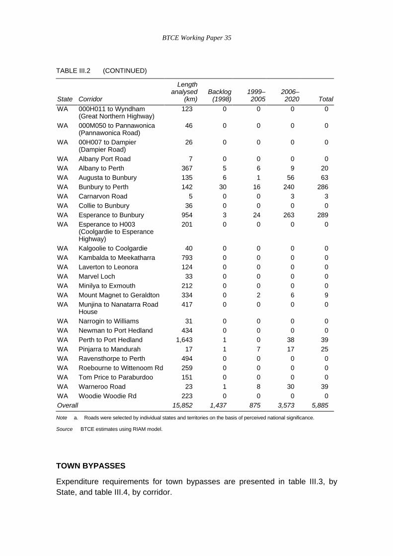
BTCE Working Paper 35
TABLE III.2 (CONTINUED)
State Corridor
Lengthanalysed
(km)Backlog
(1998)1999–2005
2006–2020 Total
WA 000H011 to Wyndham(Great Northern Highway)
123 0 0 0 0
WA 000M050 to Pannawonica(Pannawonica Road)
46 0 0 0 0
WA 00H007 to Dampier(Dampier Road)
26 0 0 0 0
WA Albany Port Road 7 0 0 0 0WA Albany to Perth 367 5 6 9 20WA Augusta to Bunbury 135 6 1 56 63WA Bunbury to Perth 142 30 16 240 286WA Carnarvon Road 5 0 0 3 3WA Collie to Bunbury 36 0 0 0 0WA Esperance to Bunbury 954 3 24 263 289WA Esperance to H003
(Coolgardie to EsperanceHighway)
201 0 0 0 0
WA Kalgoolie to Coolgardie 40 0 0 0 0WA Kambalda to Meekatharra 793 0 0 0 0WA Laverton to Leonora 124 0 0 0 0WA Marvel Loch 33 0 0 0 0WA Minilya to Exmouth 212 0 0 0 0WA Mount Magnet to Geraldton 334 0 2 6 9WA Munjina to Nanatarra Road
House417 0 0 0 0
WA Narrogin to Williams 31 0 0 0 0WA Newman to Port Hedland 434 0 0 0 0WA Perth to Port Hedland 1,643 1 0 38 39WA Pinjarra to Mandurah 17 1 7 17 25WA Ravensthorpe to Perth 494 0 0 0 0WA Roebourne to Wittenoom Rd 259 0 0 0 0WA Tom Price to Paraburdoo 151 0 0 0 0WA Warneroo Road 23 1 8 30 39WA Woodie Woodie Rd 223 0 0 0 0Overall 15,852 1,437 875 3,573 5,885
Note a. Roads were selected by individual states and territories on the basis of perceived national significance.
Source BTCE estimates using RIAM model.
TOWN BYPASSES
Expenditure requirements for town bypasses are presented in table III.3, byState, and table III.4, by corridor.

BTCE Working Paper 35
MAINTENANCE
Tables III.5, and III.6 show maintenance expenditure needs on the non-NHSroads nominated by the states and territories for analysis.
TABLE III.3 EXPENDITURE NEEDS FOR TOWN BYPASSES BY STATE ANDTERRITORY: NON–NHS ROADS
($ million)
State
Number ofbypasses
assesseda
Number ofbypasseswarranted Backlog 1999–2005 2006–2020 Total
NSW 30 10 155 38 265 458
NT 0 0 0 0 0 0
QLD 0 0 0 0 0 0
SA 6 0 0 0 0 0
TAS 1 1 0 20 16 36
VIC 22 6 14 14 71 100
WA 24 8 18 55 95 168
Overall 83 25 187 127 448 762
Note a. Roads included in this table are listed in table III.1.
Source BTCE using RIAM model.

BTCE Working Paper 35
TABLE III.4 EXPENDITURE NEEDS FOR TOWN BYPASSES BY CORRIDOR: NON–NHSROADS
($ million)
State Corridora
Number ofbypassesassessed
Number ofbypasseswarranted Backlog
1999–2005
2006–2020 Total
NSW Adelaide to Nyngan 3 0 0 0 0 0NSW Bathurst to
Cunnamulla4 1 0 0 23 23
NSW Kings Highway 1 0 0 0 0 0NSW Melbourne to Sydney
(coastal route)7 0 0 0 0 0
NSW Monaro Highway 2 0 0 0 0 0NSW Newcastle to Dubbo
(Golden Hwy)3 0 0 0 0 0
NSW Sydney to Bathurst 2 1 0 0 42 42NSW Sydney to Brisbane
(Pacific Highway)8 8 155 38 201 393
SA Adelaide to Nyngan 2 0 0 0 0 0SA Melbourne to Keith 3 0 0 0 0 0SA Port Lincoln to Port
Augusta1 0 0 0 0 0
TAS Hobart to Smithtown 1 1 0 20 16 36VIC Geelong to Benalla
(Midland Hwy)8 1 0 0 6 6
VIC Melbourne to Keith 2 0 0 0 0 0VIC Melbourne to Mildura 8 3 9 8 57 74VIC Melbourne to Sydney
(coastal route)3 2 5 7 9 20
VIC Portland to SunraysiaHwy
1 0 0 0 0 0
WA Albany to Perth 3 0 0 0 0 0WA Augusta to Bunbury 2 0 0 0 0 0WA Bunbury to Perth 2 2 18 14 21 54WA Esperance to Bunbury 11 5 0 14 53 67WA Esperance to H003
(Coolgardie toEsperance Highway)
1 0 0 0 0 0
WA Perth to Port Hedland 4 1 0 27 21 48WA Ravensthorpe to Perth 1 0 0 0 0 0Overall 83 25 187 127 448 762
Note a. Roads included in this table are listed in table III.1.
Source BTCE using RIAM model.

BTCE Working Paper 35
TABLE III.5 EXPENDITURE NEEDS FOR MAINTENANCE BY STATE AND TERRITORY: NON–NHS ROADS
($ million, 1997–98 prices)
RehabilitationResealing and routine
maintenancea All maintenance
StateLength of roadanalysedc (km)
Backlog(1998)
1999–2005
2006–2020 Total
1999–2005
2006–2020 Total
Backlog(1998)
1999–2005
2006–2020 Total
ACT 46 – 2 19 22 6 18 25 – 9 38 46
NSW 3,300 27 178 626 832 199 433 632 27 377 1,059 1,463
NT 470 – – 22 22 32 70 102 – 32 93 125
QLD 1,434 5 33 215 253 120 257 377 5 152 472 630
SA 1,023 4 6 77 87 92 204 296 4 98 281 383
TAS 247 1 4 65 70 21 43 64 1 25 108 134
VIC 2,186 15 52 511 577 165 373 537 15 216 883 1,115
WAd 7,467 1 29 415 446 530 1,166 1,697 1 559 1,581 2,142
Overall 16,172 53 304 1,951 2,308 1,165 2,564 3,729 53 1,469 4,515 6,038
Notes a. No backlog has been assumed for resealing and routine maintenance as these expenses are incurred with greater frequency than rehabilitations.
b. Dashes mean that expenditure needs are zero for the maintenance type.
c. List of routes detailed in table III.6
d. There were no roughness data for 202.09 kilometres of Western Australian non–NHS roads. Resealing and routine maintenance costs have been estimated for these sections,but not rehabilitation costs. The lengths of road lacking roughness data are: Albany to Perth 0.74km; Augusta to Bunbury 17.37km; Bunbury to Perth 32.53km; Collie to Bunbury6.5km; Esparence to Bunbury 21.1km; Kalgoorlie to Coolgardie 0.09km; Kambalda to Meekatharra 2.62km; Mount Magnet to Geraldton 8.71km; Munjina to Nanatarra RoadHouse 2.45km; Narrogin to Williams 2.18km; Newman to Port Hedland 8.13km; Perth to Port Hedland 0.05km; Ravensthorpe to Perth 84.33km; and Roebourne to Wittenoom Rd15.29km.
Source BTCE using RIAM model.

BTCE Working Paper 35
TABLE III.6 EXPENDITURE NEEDS FOR MAINTENANCE BY CORRIDOR: NON–NHS ROADS
($ million, 1996–1997 prices)
Length ofroad
RehabilitationResealing and routine
maintenancea All maintenance
State Corridorcanalysed
(km) Backlog1999–2005
2006–2020 Total
1999–2005
2006–2020 Total Backlog
1999–2005
2006–2020 Total
ACT Canberra Connections 2 – – 2 2 1 1 1 – 1 3 3ACT Kings Highway 8 – – 1 1 1 3 4 – 1 3 4ACT Monaro Highway 36 – 2 17 19 5 15 20 – 7 31 39NSW Adelaide to Nyngan 631 2 0 10 11 32 69 102 2 32 79 113NSW Bathurst to Cunnamulla 801 4 10 65 79 40 89 129 4 50 154 208NSW Kings Highway 128 3 5 29 36 9 18 27 3 14 47 63NSW Melbourne to Sydney
(coastal route)429 5 38 161 203 30 65 95 5 68 226 299
NSW Monaro Highway 206 1 3 37 40 14 30 44 1 17 67 84NSW Newcastle to Dubbo
(Golden Hwy)313 – 9 54 64 16 35 51 – 26 89 115
NSW Sydney to Bathurst 91 – 7 41 48 9 19 27 – 15 60 75NSW Sydney to Brisbane (Pacific
Highway)700 13 107 229 348 49 108 157 13 156 337 505
NT Arnhem Hwy 223 – – 22 22 15 34 48 – 15 56 71NT Stuart Hwy to Ayers Rock 247 – – – – 17 37 54 – 17 37 54QLD Brisbane to Darwin 14 – – – 1 1 2 3 – 1 3 4QLD Rockhamption to
Barcaldine575 1 9 65 75 41 90 130 1 50 155 206
QLD Sydney to Brisbane(Pacific Highway)
83 3 21 108 131 25 44 69 3 46 152 200
QLD Townsville to Cloncurry 763 1 2 42 45 53 121 174 1 55 163 219SA Adelaide to Nyngan 380 1 2 11 13 33 74 108 1 35 85 121SA Melbourne to Keith 232 – 2 50 52 22 49 71 – 24 99 123SA Pimba to Olympic Dam 94 – – – – 9 20 29 – 9 20 29

BTCE Working Paper 35
TABLE III.6 (CONTINUED)
Length ofroad
RehabilitationResealing and routine
maintenancea All maintenance
State Corridoranalysed
(km) Backlog1999–2005
2006–2020 Total
1999–2005
2006–2020 Total Backlog
1999–2005
2006–2020 Total
SA Port Lincoln to PortAugusta
317 3 2 16 21 27 61 89 3 29 77 110
TAS Cygnet to Hobart 46 – 1 14 15 5 9 13 – 5 23 28TAS Hobart to Smithtown 97 – 1 23 24 8 16 24 – 9 39 48TAS Launceston to Georgetown 47 – 1 17 17 4 10 14 – 5 26 31TAS Triabunna to Hobart 57 – 2 12 14 4 9 13 – 6 21 27VIC Geelong to Benalla
(Midland Hwy)420 4 9 60 74 29 66 95 4 38 126 168
VIC Melbourne to Keith 410 2 8 104 114 31 71 102 2 39 175 216VIC Melbourne to Mildura 548 5 10 101 117 39 89 129 5 49 191 246VIC Melbourne to Sydney
(coastal route)470 3 22 230 255 46 101 148 3 68 332 403
VIC Portland to Sunraysia Hwy 337 1 2 15 18 20 44 64 1 22 60 82WA 000H006 to Broome
(Broome Highway)42 – – 4 4 3 6 9 – 3 10 14
WA 000H006 to Derby(Derby Highway)
43 – – 1 1 3 7 10 – 3 7 10
WA 000H006 to Port Hedland(Port Hedland Road)
10 – – – – 1 2 3 – 1 2 3
WA 000H007 to Karratha(Point Samson toRoebourne Road)
18 – – – – 2 3 5 – 2 3 5
WA 000H011 to Wyndham(Great Northern Highway)
123 – – 4 4 9 21 30 – 9 24 34
WA 000M050 to Pannawonica(Pannawonica Road)
46 – – – – 4 8 11 – 4 8 11

BTCE Working Paper 35
TABLE III.6 (CONTINUED)
Length ofroad
RehabilitationResealing and routine
maintenancea All maintenance
State Corridoranalysed
(km) Backlog1999–2005
2006–2020 Total
1999–2005
2006–2020 Total Backlog
1999–2005
2006–2020 Total
WA 00H007 to Dampier(Dampier Road)
26 – – 1 1 2 5 7 – 2 6 8
WA Albany Port Road 7 – – – – 1 1 2 – 1 1 2WA Albany to Perthd 374 – 1 59 61 33 76 109 – 34 136 170WA Augusta to Bunburyd 141 – 4 42 45 17 38 55 – 20 80 100WA Bunbury to Perthd 155 – 2 79 81 17 36 52 – 19 115 134WA Carnarvon Road 5 – – 1 1 1 2 3 – 1 3 4WA Collie to Bunburyd 36 – – 8 8 4 9 13 – 5 17 22WA Esperance to Bunburyd 987 1 19 129 148 74 161 235 1 92 290 383WA Esperance to H003 205 – – 2 2 17 38 55 – 17 40 57WA Kalgoolie to Coolgardied 40 – – – – 4 9 14 – 4 9 14WA Kambalda to Meekatharrad 793 – – 2 3 45 97 142 – 45 100 145WA Laverton to Leonora 124 – – – – 10 21 31 – 10 21 31WA Marvel Loch 33 – – 3 3 2 5 7 – 2 8 10WA Minilya to Exmouth 212 – – – – 17 36 53 – 17 36 53WA Mount Magnet to
Geraldtond334 – – 7 7 26 56 82 – 26 63 89
WA Munjina to Nanatarra RoadHoused
417 – – – – 19 41 60 – 19 41 60
WA Narrogin to Williamsd 31 – – 1 1 3 6 8 – 3 7 10WA Newman to Port Hedlandd 434 – – – – 7 16 23 – 7 16 23WA Perth to Port Hedlandd 1,662 – 2 47 49 140 308 449 – 142 356 498WA Pinjarra to Mandurah 17 – – 11 11 9 20 30 – 9 31 40WA Ravensthorpe to Perthd 495 – – 8 8 32 70 102 – 32 78 110WA Roebourne to Wittenoom
Rdd259 – – – – – – – – – – –

BTCE Working Paper 35
TABLE III.6 (CONTINUED)
Length ofroad
RehabilitationResealing and routine
maintenancea All maintenance
State Corridoranalysed
(km) Backlog1999–2005
2006–2020 Total
1999–2005
2006–2020 Total Backlog
1999–2005
2006–2020 Total
WA Tom Price to Paraburdoo 151 – – – – 10 22 33 – 10 22 33WA Warneroo Road 23 – – 6 6 2 5 7 – 2 11 13WA Woodie Woodie Rd 223 – – – – 17 40 57 – 17 40 57
Overall 16,172 53 304 1,951 2,308 1,165 2,564 3,729 53 1,469 4,515 6,038
Notes a. No backlog has been assumed for resealing and routine maintenance as these expenses are incurred with greater frequency than rehabilitations.
b. Dashes mean that expenditure needs are zero for the maintenance type.
c. List of routes detailed in table III.6
d. There were no roughness data for 202.09 kilometres of Western Australian non–NHS roads. Resealing and routine maintenance costs have been estimated for these sections,but not rehabilitation costs. The lengths of road lacking roughness data are: Albany to Perth 0.74km; Augusta to Bunbury 17.37km; Bunbury to Perth 32.53km; Collie to Bunbury6.5km; Esparence to Bunbury 21.1km; Kalgoorlie to Coolgardie 0.09km; Kambalda to Meekatharra 2.62km; Mount Magnet to Geraldton 8.71km; Munjina to Nanatarra RoadHouse 2.45km; Narrogin to Williams 2.18km; Newman to Port Hedland 8.13km; Perth to Port Hedland 0.05km; Ravensthorpe to Perth 84.33km; and Roebourne to Wittenoom Rd15.29km.
Source BTCE using RIAM model.

BTCE Working Paper 35
APPENDIX IV ADEQUACY OF AUSTRALIAN BRIDGES
Except for those spanning significant geographic features, bridges tend toattract little interest from road users. However, they are more numerous thancommonly supposed and are an essential component of the road infrastructure.
Bridges are relatively more expensive to construct than road pavements, andare therefore designed for a longer service-life. Failure of a bridge has moresevere consequences than a road failure, none more spectacularly illustratedthan by the loss of 3 spans of the Tasman Bridge in Hobart because of a shipcollision in 1975.
The range of ages and strengths in Australia’s bridge infrastructure reflects thelonger service life of bridges and the increase over time in the mass andnumber of heavy vehicles. For example, bridges presently in service onnational highways were designed and constructed over 50 years ago for loadshalf the size of the loads applied by contemporary heavy vehicles. It is thestrength of these older bridges that limits the potential productivityenhancements associated with increased heavy vehicle weights.
CHARACTERISTICS OF BRIDGES ANALYSED
Designated Network
The analysis was undertaken on a designated primary road network. Thenetwork consisted of National Highways and other primary rural roads as listedin table 2.1
The bridge inventory available was a combination of selected parts of thebridge inventory collected for the Mass Limits Review (NRTC 1996a) and datacollected specifically for the project.
The material in this appendix is reproduced with minor editorial changes from a reportprepared under contract to the BTCE by Dr Rob Heywood (Queensland University ofTechnology) and Bob Pearson (Pearsons Transport Resource Centre P/L).

BTCE Working Paper 35
TABLE 2.1 PRIMARY ROAD NETWORK
National Highways1
CorridorTotal length
(km) Note
Sydney-Melbourne 804Canberra connections 121Sydney-Brisbane (New England Hwy) 914Sydney-Adelaide (Sturt Hwy) 1,001 Tarcutta (Hume Hwy) to Adelaide
(Cavan)Melbourne-Adelaide 716Melbourne-Brisbane (Newell Hwy) 1,441 Seymour to ToowoombaBrisbane-Cairns 1,699Adelaide-Perth 2,671Adelaide-Darwin 2,695 Port Augusta to DarwinPerth-Darwin 3,708 Midland (Perth) to KatherineBrisbane-Darwin 2,433 Brisbane to Threeways Roadhouse
(Tennant Creek)Hobart-Burnie 333 The route length between Hobart and
Burnie is 320km. There is also 13kmof parallel roadway declared as aNational Highway
Total 18,536
Other primary roads
CorridorTotal length
(km) Note
Sydney-Melbourne (Princes Hwy) 975Sydney-Brisbane (Pacific Hwy) 794 Newcastle (Hexham) to BrisbaneSydney-Adelaide (via Broken Hill) 1,093 NSW highways onlyMelbourne-Mt Gambier 385 Princes Hwy West in Victoria onlyMelbourne-Mildura 535Perth-Port Hedland (via Geraldton) 1,704 North West Coastal Hwy & Brand HwyPerth-Coolgardie (via Albany) 1,204Total 6,690
Note 1. Excludes any national highways in the urban area.
Source Table 2.7 BTCE (1994) and consultants’ derivation.
The Mass Limits Review inventory was not road or bridge specific, butaggregated data by State and Territory in the categories of National Highwaysand Rural Arterials with traffic volumes greater than 5,000 vehicles per day(vpd). Where assessment of specific corridors was required, estimates weremade based on:
• number of bridges or deck area in each corridor (where available); or
• carriageway length adjusted by type of terrain.

BTCE Working Paper 35
TABLE 2.2 NUMBERS OF BRIDGES IN THE PROJECT INVENTORY
State
NSW VIC QLD SA WA TAS NT ACT Aust
National Highways 462 255 681 3281 105 73 72 0 1976
Other primary roads 209 162 0 0 101 0 0 0 472
Note 1. Including 205 ‘bridges’ in South Australia which have spans less than 5m.
Bridge Inventory on Designated Network
The inventory contains information on 2448 bridges in all States and theNorthern Territory (table 2.2). It should be noted that the majority of the bridgesin the South Australian bridge inventory have spans less than 5 m (205
or 63 per cent) whereas the inventory in all other states shows much smallernumbers in this span range. This is a reflection of varying policies regarding thedefinition of what constitutes a bridge with many States regarding thesestructures as culverts.
The bridges included in the inventory represent a total deck area of1,553,000 m2 with an estimated replacement cost of $1,900 million, of which$1,500 million is for national highways.
The inventory contained information on numbers of bridges and deck areas inthe following categories:
• road classification;
• superstructure material;
• type of superstructure;
• simply supported or continuous;
• span length of the maximum span;
• design load (a surrogate for age); and
• condition.
A distinction was made between simply supported and continuous bridgesbecause of the differences in the way that they respond to modern vehicles.Simply supported bridges have beam elements which span between piers witha joint over each pier. In contrast the beam elements of continuous bridgescontinue over each pier thus eliminating the joint but introducing another regionwhich is sensitive to modern vehicles which are both heavier and longer thanthe original design loads.

BTCE Working Paper 35
FIGURE 2.1 BRIDGE CONDITION ON RURAL NATIONAL HIGHWAYS - PERCENTAGEBY NUMBER
Condit ion
0%
20%
40%
60%
80%
100%
N S W VIC QLD SA W A TAS N T ACT AUST
Good Fair Poor
Bridges on National Highways
Condition
Bridges on National Highways are generally in good condition, with 94 per centclassified in this category. Figure 2.1 shows that New South Wales,Queensland, Western Australian and South Australian bridges are virtually allin good, condition. Victoria has the lowest proportion of bridges in goodcondition being 82 per cent, while Northern Territory has the highest proportionof bridges in poor condition.
Design standard (Age)
The design standard is used as a surrogate for age as well as the fundamentalindicator of bridge strength. Three design load groupings are considered. Theyare denoted by the nomenclature used in the appropriate bridge design code.T44 denotes bridges built since 1976, MS18 denotes bridges built between1948 and 1976, and pre MS18 are pre 1948 bridges. The latter group covers awide variety of design standards, a history of which can be found in the Reviewof Road Vehicle Limits (NAASRA 1985). The T44, MS18 and other relatedbridge design loads are summarised in Appendix A.
On National Highways, 43 per cent of bridges were designed and built in thelast 20 years to T44 design standard. Of the remainder, 46 per cent were builtto MS18 and 11 per cent to earlier standards.
The Northern Territory has the highest percentage of bridges built to T44 (64per cent) and also the highest percentage of pre 1948 bridges (18 per cent). Asillustrated in figure 2.2, Victoria and Tasmania have the lowest proportion ofmodern bridges (less than 40 per cent) and are the only States less than thenational average. In each case, they also have the highest proportion of MS18

BTCE Working Paper 35
bridges at 56 per cent. South Australia has the lowest proportion of pre 1948bridges at 4 per cent.
FIGURE 2.2 DESIGN STANDARDS (AGE) OF STATE/TERRITORY BRIDGES ON RURALNATIONAL HIGHWAYS - PERCENTAGE BY NUMBER
D e s ign s tandard
0%
20%
40%
60%
80%
N S W V IC QLD SA W A T A S N T ACT A U S T
T44 MS18 PreMS18
Span length
Apart from the Northern Territory, the span lengths of bridges exhibit areasonably consistent pattern. In the Northern Territory, 69 per cent of bridgesare in the range 9m to 11m. No other State or Territory has any one span rangerepresented in more than 30 per cent of bridges. New South Wales, Victoriaand South Australia have the highest proportion (>19 per cent) of bridges withmore than 30m spans. On a national basis, the highest proportion of bridges(22 per cent) is in the 9m to 11m range, with Tasmania, Queensland, NewSouth Wales and of course Northern Territory all having high proportions ofbridges in this range.
However, when deck area is used as the measurement parameter, the longerspans take on more prominence. Sixty percent of the deck area of Australia’sbridges on National Highways span more than 20m compared to 35 per cent ofthe bridge population. table 2.3 shows the position.

BTCE Working Paper 35
TABLE 2.3 BRIDGES BY SPAN AND STATE
(per cent)
NSW VIC QLD SA1 WA TAS NT Aust
N DA N DA N DA N DA N DA N DA N DA N DA
≤5m 0 0 7 2 1 0 7 4 3 1 11 1 0 0 5 1
5-7m 9 4 7 3 4 1 6 2 25 13 14 4 0 0 9 3
7-9m 10 6 5 1 6 3 9 4 11 10 14 8 0 0 9 5
9-11m 19 13 16 12 22 14 6 4 21 14 23 19 69 51 22 15
11-13m 8 4 11 11 14 11 6 4 5 6 7 6 1 1 9 7
13-15m 7 5 7 9 19 18 15 7 3 2 5 7 8 3 10 9
15-20m 16 16 16 21 14 16 19 18 30 49 12 22 11 11 15 19
20-30m 20 21 12 27 18 27 23 31 2 5 12 23 7 28 15 24
>30m 9 31 9 14 2 10 10 26 0 0 3 11 3 7 5 17
Unknown - - 11 - - - - - - - - - - - 1 -
Notes N = number
DA = deck area
1. excluding the 205 culverts
FIGURE 2.3 SUPERSTRUCTURE MATERIAL
Superstructure Material
0%
20%
40%
60%
80%
100%
NSW VIC QLD SA WA TAS NT ACT AUST
Steel Timber Rconc Pconc Other
TABLE 2.4 COMPARISON OF BRIDGES ON NATIONAL HIGHWAYS WITH OTHERBRIDGES ON THE DESIGNATED NETWORK
(per cent)
Design standard Condition
T44 MS18 pre MS18 good fair poor
National Highways 43 46 11 94 5 1
Other primary roads 35 44 22 85 14 1

BTCE Working Paper 35
Superstructure material
Concrete is the predominant superstructure material, with more than 60 percent of Australian bridges on National Highways being constructed ofprestressed concrete and 20 per cent of reinforced concrete. New SouthWales, Queensland and Northern Territory all have more than 80 per cent oftheir bridges made of concrete. Steel comprises 18 per cent of superstructurematerial and timber 3 per cent when measured by bridge numbers.
Bridges on other primary roads
In general, bridges on other primary roads are older, not in as good a conditionand have similar span lengths and construction materials. The comparison ofdesign standard (age) and condition is given in table 2.4.
Bridge Loading
The bridge analysis considered three different mass limit scenarios. Indetermining these scenarios, historical trends in mass limits were examined.
Each State and Territory prescribes the maximum legal limits for the allowablemass on road vehicles. Limits are placed on each axle, axle group and thegross or total laden vehicle mass. Up until 1977, every State and Territory haddifferent allowable mass limits. Following the NAASRA Economics of RoadVehicle Limits Study (Fry et al 1975), the eastern and western regions ofAustralia were basically uniform within each region but with the western Statesbeing higher. Only in 1988 were the legal mass limits for heavy vehiclesuniform across Australia when the 42.5 tonne gross mass limit of option C ofthe RoRVL Study (NAASRA 1986a) was adopted.
The types of vehicles have also changed over recent years. Up until 1976,triaxles were rare, and the basic long distance vehicle was either a 4 or 5 axlearticulated. Since 1977, the 6 axle articulated vehicle has been the commonlong distance eastern seaboard vehicle, with double or triple road trainsoperating in more remote parts of the nation.
Since their introduction in the 1980s, B-doubles have taken an increasingproportion of the long distance eastern seaboard freight and now carry anestimated 15 per cent of this traffic.
From a bridge perspective, the critical vehicle depends upon the span of thebridge. The spans and the critical axle groups on vehicles are:
• less than 13m triaxles;
• 13m to 30m 6 axle articulated vehicles; and
• above 30m B-double.
The historical trend in legal gross mass in Victoria for articulated vehicles isillustrated in figure 2.4. These trends are generally representative of limits inthe eastern states and, while pre 1988 limits were lower than the western

BTCE Working Paper 35
region of Australia, are sufficiently representative to make predictions of futurelimits (see Section 3.4). It is interesting to contrast the changes in limits to thechanges in bridge design loads (figures 2.5 and 2.6).
FIGURE 2.4 TREND IN VICTORIAN MASS LIMITS (TONNES)
0
510
1520253035
4045
1950 1955 1960 1965 1970 1975 1980 1985 1990 1995
yea r
gros
s m
ass
(t)
t rend
l e g a l m a s s

BTCE Working Paper 35
FIGURE 2.5 TRENDS IN BRIDGE DESIGN LOADS IN AUSTRALIA - COMPARISON OFBENDING MOMENTS INDUCED IN A 15 M SIMPLE SPAN
Year
Bending Moment
(kNm)
0
200
400
600
800
1000
1200
1900 1920 1940 1960 1980 2000
NSW
Vic
SA
Qld
Aust
Trend
T44
HS20 - MS18
FIGURE 2.6 COMPARISON OF SELECTED BRIDGE DESIGN LOADS WITH CURRENTT44 BRIDGE DESIGN LOAD
0
0.2
0.4
0.6
0.8
1
1.2
1.4
1.6
0 25 50 75 100Simple Span [m]
Mid
span
Mo
men
t /
T44
Mid
span
Mo
men
t
T44 1975-
MS18(HS20) 1948-75
Road Train 16t @ 21'
AA 1936-47
DMR 1927-38
A-1st Class 1920-47
Figure 2.5 compares the bridge design loads on the basis of the effects(bending moments) they induce in a 15 m span. Figure 2.6 shows that ratio ofeffects induced by different design loads to the current T44 bridge design loadvaries significantly with span.

BTCE Working Paper 35
Bridge Expenditure
Maintenance
Maintenance costs are associated with a broad range of activities. Theseinclude periodic inspections, painting, waterway clearing, guardrail repair, deckjoint maintenance, replacement of elements damaged by impact of vehicles andthe like.
The maintenance cost varies dramatically with construction material and to alesser extent with geographical location. The maintenance costs associatedwith timber bridges are very significant as a major deck rehabilitation is usuallyrequired every 7 to 10 years. Consequently the maintenance cost of traditionaltimber girder bridges is at least an order of magnitude larger than thoseassociated with reinforced concrete bridges for example. The number ofbridges that are included in the inventory associated with this project is small (4per cent by number) and they are identified for replacement relatively quickly.Thus it is assumed that the timber bridges will be replaced rather thanmaintained leaving the inventory with lower maintenance bridges.
The maintenance cost will be substantially lower on the major highways due tothe fact that the bridges are newer. The bridge replacement model developedfor this project also assumes that bridges are replaced rather than accept anincreased maintenance/strengthening scenario. In this way the bridge inventorywill remain in good condition and the maintenance costs low.
Based on discussions with road authorities, maintenance costs of bridges ingood condition have been estimated at approximately $600 per bridge per yearwith an accuracy of ±20 per cent.
Widening
Bridge widening is a relatively expensive activity from a bridge standpoint but issometimes the most cost effective solution compared with a new bridge. Thereduced cost of approaches plays a significant part in the savings. Theincreased costs are associated with need to break into existing construction, tooperate under and near traffic together with the limited opportunities foreconomies of scale.
The general preference is not to widen bridges. The cost of widening is not welldocumented and varies significantly from bridge to bridge. The relationship forwidening costs presented in figure 2.7 has been normalised against the cost ofthe equivalent new construction of the structure being widened. The economiesof scale improve with the width of the widening. The widening cost index CW isdefined as follows:

BTCE Working Paper 35
FIGURE 2.7 COST OF BRIDGE WIDENING
CW =Cost of widening per m
Cost of new construction per m
2
2
Width of widening [x]
Cw
Cw = 0.02(x-10)2 + 1.2 > 1.2
3.0
2.0
1.0
Hence the cost of widening can be estimated as follows:
Cost of widening =C x Area of widening x Unit rate for the equivalent new constructionw
The costs associated with widening have not been included in the costs ofupgrading the bridge infrastructure.
EVALUATING BRIDGES
The database for the bridge evaluation model was a modified version of theinventory used in the National Road Transport Commission (NRTC) MassLimits Review last year. It covered bridges on the following roads:
• National Highways;
• Rural Arterials carrying more than 5000 vehicles per day; and
• other roads where information was provided by States.
The data is disaggregated by:
• road classification;
• superstructure material;
• type of superstructure;
• simply supported or continuous;
• span length of the maximum span;
• design load (a surrogate for age); and
• condition.

BTCE Working Paper 35
For more details of the disaggregation, refer to pp B.4 and B.5 of NRTC(1996b).
Loading Scenarios
The history of mass limits for trucks in Australia (outlined above) was used todevelop three different mass limit scenarios used in the bridge analysis.
It appears likely that option F of the Mass Limits Review (NRTC 1996) will beadopted in the relatively near future. The articulated vehicle limits of45.5 tonnes for option F was therefore adopted as the base case.
For the purposes of assessing future limits, the recent trend to increase masslimits every decade provides the basis for the three scenarios adopted. Thesescenarios are:
Scenario 1: gross mass 45.5 tonnes, no future increases;
Scenario 2: gross mass 45.5 tonnes, increasing to 52 tonnes in 2010, noother increases; and
Scenario 3: as for scenario 2, but a further increase to 58 tonnes forarticulated vehicles in 2020.
These scenarios are for bridge impact calculations only and incrementsbetween these years will have a minimal effect on the results.
The 58 tonne limit is slightly in excess of the trend line but was chosenbecause it coincides with a mass for which independent cost estimates will beavailable (Pearson and Bayley 1997).
The detailed scenarios are as given in table 3.1 and illustrated in figure 3.1.
The reporting periods for the cost of bridge replacements are also indicated infigure 3.1 by the vertical lines. The four costing periods are defined as follows:
1. Current (1997);
2. 1998 - 2005;
3. 2006 - 2020; and
4. 2021 - 2030.
Pavement implications have not been considered in this exercise. It is possiblethat additional axles may be necessary to reduce pavement wear, but for themajority of cases little effect results for bridge costs.
Other important assumptions were that:
• greater increases are assigned to triaxles compared to tandem axles so thatload per axle is approaching the same for tandem and triaxles;
• tyre capacities are available to carry the loads; and

BTCE Working Paper 35
• both air suspensions and mechanical suspensions will be represented in thefleet in future years (important for bridge dynamic effects).
TABLE 3.1 BRIDGE LOADING SCENARIOS
Scenario Years Design Vehicle
1 1997 on Artic 0 00 0006 17 22.5
B-double 0 00 000 0006 17 22.5 22.5
2 1997 to 2010 Artic 0 00 0006 17 22.5
B-double 0 00 000 0006 17 22.5 22.5
2010 on Artic 0 00 0006.5 19 26.5
B-double 0 00 000 0006.5 19 26.5 26.5
3 1997 to 2010 as above
2010 to 2020 as above
2020 on Artic 0 00 0006.5 20.5 31
B-double 0 00 000 0006.5 20.5 31 31

BTCE Working Paper 35
FIGURE 3.1 BRIDGE LOADING SCENARIOS AND COSTING PERIODS
B-double
Six-axlearticulated
Triaxle group
Steer axle
Tandem group
Period 3 Period 4Period 2
0
10
20
30
40
50
60
70
80
90
100
1990 2000 2010 2020 2030 2040 2050Year
Mas
s [t
] Scenario 3Scenario 2Scenario 1
Bridge Evaluation Model
The model used to predict the remaining life of Australia’s bridges is anadaptation of the model developed by R. Wedgwood and the AUSTROADSteam for the Mass Limits Review. It is based largely on limit state designconcepts, historical information, research findings and knowledge relating tothe performance of bridges over the years. Like most complex models, itinvolves many approximations and general assumptions. More sophisticatedmethods applied to individual bridges could well extend or reduce the life of anindividual bridge compared with the model. However, the model is consideredto provide an acceptable indication of the expenditure required for Australianbridges.
Bridges can fail in many ways. However, they are usually designed so thatshould they fail then the failure will occur in a controlled ductile manner. Ductilefailures are generally associated with bending effects and thus a well designedbridge will fail in bending first. As a consequence, the bridge evaluation modelis based around the bending effects induced by traffic.
Bending moments in bridges are calculated from the wheel loads applied to thebridge. Consider the simple span and the vehicle illustrated in figure 3.2. Theinternal shear (V) and bending moments (M) can be calculated at a point (A-A)

BTCE Working Paper 35
from the calculated reactions (R) and the positions (a1, a2, a3, b) of the wheelloads (P1, P2, P3) as follows:
V = R - P1 - P2 - P3
M = Rb - (P1a1 + P2a2 + P3a3)
The bridge evaluation model includes a comparison of the bending momentsinduced by current or future heavy vehicles compared with the bendingmoments that the bridge was designed to resist.
Australian bridge design codes have adopted the limit state concept for bridgedesign since 1976. Prior to this time, bridges were designed based on workingstress methods. In this case the dead load (or self weight effects) plus the liveload (or traffic) effects were not permitted to exceed an allowable stress whichwas typically some form of yield strength reduced by a factor of safety or safetymargin. Thus the safety margin was the same for the dead load and the liveload.
FIGURE 3.2 BENDING MOMENTS AND SHEARS INDUCED IN SIMPLY SUPPORTEDBRIDGES
P1 P2 P3
M
V
ba1
a2
a3
Span
A
A
R
FIGURE 3.3 WORKING STRESS DESIGN METHODS USED PRIOR TO 1976 (I.E. MS18LOADS AND EARLIER)
QLive loadeffects
SafetyMargin
Yield
GDead load
effects

BTCE Working Paper 35
The objective of bridge design and the limit state concept is to ensure that thebridge fulfils its purpose and ensures that the probability of failure isacceptable. The AUSTROADS Bridge Design Code expresses this in terms ofthe load and resistance (strength) of the bridge. The probability of failure isdeemed to be acceptable if the estimated extreme event during the life time ofthe bridge is smaller than a lower bound estimate of the strength of the bridge.Mathematically this limit state equation is expressed as follows:
Extreme loading ≤ lower bound estimate of strength
aGG + aQQ ≤ fRu
where:
aG load factor for dead load (1.25 typically)
G effects induced by dead loads (including an allowance forsuperimposed dead loads such as asphalt surfacing)
aQ load factor for live load (2.0 for traffic loads)
Q effects induced by live load (including the dynamic load allowance)
f strength reduction factor
Ru ultimate strength (characteristic)
In limit state design the safety margins associated with dead load aresubstantially smaller than that associated with live loads. This contrasted witholder working stress design methods which effectively allocated the samesafety margin to both dead and live loads. Thus the introduction of limit statedesign concepts permitted an increase in live loading for existing bridges.
FIGURE 3.4 LIMIT STATE DESIGN CONCEPTS USED SINCE 1976 (I.E. T44 LOADING)
1.25G 2Q
Ru
φRu
(1−φ)Ru
In addition, experience has shown that the performance of bridges in goodcondition is often better than was anticipated based on the original design

BTCE Working Paper 35
calculations. For example, a recent test of a Victorian bridge to failure showedthat the bridge was substantially stronger than the original calculationsindicated. Also the actual effects induced in the bridge by the traffic aredifferent to those predicted by the appropriate bridge design load. These twogroups of influences can be included in the limit state equation through theapplication of a live load modification factor (kQ) and a resistance modificationfactor (ku):
aGG + aQkQQ ≤ fkuRu
Through the adoption of safe but conservative assumptions during the designphase, the resistance is often greater than expected (i.e. ku > 1.0). Likewise theactual effects induced by the traffic loading are generally smaller than thoseinduced (by theoretical calculation) by the design loading (i.e. kQ < 1.0). Theresult is some reserve capacity when a structure is new.
Over time, the traffic loads increase and the strength of the structure candeteriorate due to corrosion and the like. As a consequence the live loadmodification factor (kQ) increases and the resistance modification factor (ku)reduces. Figure 3.6 presents this scenario for a particular value of the live loadfactor aQ that satisfies the limit state equation. The value of this live load factoris then used to determine the remaining life of the structure.
FIGURE 3.5 NEW BRIDGES OFTEN HAVE RESERVE CAPACITY AVAILABLE THAT CANFACILITATE INCREASES IN LOAD CARRYING CAPACITY
kuRu
φkuRu
1.25G 2kQQ(1−φ)kuRu
ReserveCapacity
By dividing the limit state equation by (G+Q) and noting that:
FG = G/(G+Q)
FQ = Q/(G+Q) gives:
aGFG + aQkQFQ ≤ fkuRu/(G+Q)

BTCE Working Paper 35
This equation can be re-arranged to give the live load factor aQ which usuallyhas a value aQ ≈ 2 assuming the bridge design live load is representative of thetraffic loading.
αφ α
Qu u
Q Q
G G
Q Q
k R
k F G Q
F
k F≤
+−
( )
The model used to determine the remaining life of the bridge is derived fromthe value of aQ. The live load modification factor (kQ) and a resistancemodification factor (ku) are detailed below.
Live load modification factor (kQ)
The live load modification factor (kQ) is expressed as follows:
kQ = kQ1 kQ1ckQ2kQ3kQ4 kQ5
where the sub-factors are described below and then defined.
kQ1 Bridge design vehicle factor
kQ1c Continuity load factor
kQ2 Legal load factor
kQ3 Bridge response factor
FIGURE 3.6 THE STRENGTH LIMIT STATE INCORPORATING ALLOWANCES FORINCREASED LOADS AND DETERIORATION IN THE STRENGTH
kuRu
φkuRu
αGG αQkQQ(1−φ)kuRu
kQ4 Bridge design code factor
kQ5 Bridge profile and truck suspension factor.
These factors are designed firstly to investigate the effects of increases inloads on the bridges and secondly to incorporate some factors that have beenobserved in the field that help explain the often enhanced performancecompared with bridge design code provisions. These are detailed below:
kQ1 Bridge design load factor

BTCE Working Paper 35
This factor allows for the increases in design load used to design the bridge tothe current traffic loading (refer figure 2.5 and 2.6). This involves an adjustmentdue to increases in bridge design load and a factor relating to the fact that thecurrent traffic loading (RoRVL C) is not uniformly represented by the T44design vehicle (Heywood, 1993 & 1995).
TABLE 3.2 BRIDGE DESIGN LOAD FACTOR (KQ1)
Span (m) Pre MS18 MS18 T44
<5 1.38 1.16 1.10
5-7 1.50 1.17 1.05
7-9 1.47 1.14 0.97
9-11 1.43 1.17 0.90
11-13 1.42 1.16 0.88
13-15 1.43 1.13 0.86
15-20 1.42 1.16 0.88
20-30 1.36 1.27 0.95
>30 1.25 1.33 1.00
Unknown - - -
kQ1 =
=
Effects induced in simply supported bridges by RoRVL C trafficEffects induced in simply supported bridges by the bridges' design load
function of (Bridge Design Load, Span)
As with the Mass Limits Review, three categories of bridge design load havebeen adopted. The recommended values for kQ1 are as follows. (Please notethat the values for spans larger than 30 m can vary quite significantly. Aconservative value has been adopted. It should be further noted that thenumber of bridges in this category that will require replacement is relativelysmall although their cost impact could be significant.)

BTCE Working Paper 35
TABLE 3.3 CRITICAL DESIGN LOADS AND KQ2 FACTORS BY SPAN
Truck configurations and loads Critical design loads by span
o oo ooo o oo ooo o oo ooo ooo <13 13-30 >30
A42.5 6.0 16.5 20.0 42.5 62.5 20.0 42.5 62.5
A45.5 6.0 17.0 22.5 45.5 68.0 22.5 45.5 68.0
A52.0 6.5 19.0 26.5 52.0 78.5 26.5 52.0 78.5
A58.0 6.5 20.5 31.0 58.0 89.0 31.0 58.0 89.0
kQ2 by span
A42.5 6.0 17.0 22.5 45.5 68.0 1.00 1.00 1.00
A45.5 6.0 17.0 22.5 45.5 68.0 1.13 1.07 1.09
A52.0 6.5 19.0 26.5 52.0 78.5 1.33 1.22 1.26
A58.0 6.5 20.5 31.0 58.0 89.0 1.55 1.36 1.42
TABLE 3.4 BRIDGE RESPONSE FACTOR (KQ3)
Span (m) TimberTimberTruss
ReinforcedConcrete
PrestressedConcrete Steel
SteelTruss
1 <5 .90 1.0 .90 .90 .90 .95
2 5-7 .90 1.0 .90 .90 .90 .95
3 7-9 .90 1.0 .90 .90 .90 .95
4 9-11 .90 1.0 .90 .90 .90 .95
5 11-13 .90 1.0 .90 .90 .90 .95
6 13-15 .90 1.0 .95 .95 .95 .95
7 15-20 1.0 1.0 .95 .95 .95 1.00
8 20-30 1.0 1.0 .95 .95 .95 1.00
9 >30 1.0 1.0 1.00 1.00 1.00 1.00
10 Unknown - - -
kQ1c Bridge design load continuity factor
The effects induced in short span continuous bridges have traditionally beenunderestimated in comparison to the effects induced by legal vehicles. Thiseffect is included in the model through the adoption of the continuity factor(Fcont) from the Mass Limits Review.
kQ2 Legal load factor

BTCE Working Paper 35
kQ2 =
=
Effects induced by proposed legal vehiclesEffects induced by the RoRVL C legal vehicles
function of (Span,Gross vehicle mass, Axle group loads, axle spacing)
This factor incorporates the increases in legal loads over time by scaling thelive load up in comparison to the RoRVL C limits (the limits adopted followingthe Review of Road Vehicle Limits Study in 1985). The scaling factor is basedon the axle group loads which are critical for the span under consideration. Thevalues of kQ2 are summarised in table 3.3.
kQ3 Bridge response factor
kQ3 =
=
Actual bridge responseTheoretical bridge response
function of (Structure type, span, bearing restraint,
membrane action, analytical model...)
kQ4 Bridge design code factor
This factor is designed to compensate for the fact that bridge design codeprovisions are based around heavily trafficked routes rather than the mostlylightly trafficked highways in Australia. The assumptions relating to the numberof vehicles present on a bridge at any one instant and their positioningrequirements are compensated for as a function of traffic volume. The type ofhighway is used here as a surrogate for traffic volume although there are someparts of the national highway which are less heavily trafficked than the majorarterial roads.
kQ 4 =
=
Actual effects induced by traffic streamEstimated effects induced by traffic stream (Code approx)function of (Span, Traffic volume, lateral position, multiple presence...)
= 0.95 for National Highways
= 0.90 for Major Arterial Roads
= 0.80 for lightly trafficked local roads
kQ5 Bridge profile and truck suspension factor.
kQ5 =
=
≈
Actual dynamic effects induced by traffic streamEstimated effects induced by traffic stream (Code approx)
function of (Road profile; vehicle suspension; bridge frequency,
stiffness & damping)
function of (Road Class, vehicle suspension, bridge type, bridge span)

BTCE Working Paper 35
TABLE 3.5 VALUES OF KQ5 USED IN THE EVALUATION MODEL
Span
Timber (non-composite)
Steel(composite)
averagedamping
Steel (non-composite)v. strongdamping
Reinforcedconcrete strong
damping
Prestressedconcrete average
damping
(m) S* R* S R S R S R S R<7 - - - - - - - - - -7-13 - - 1.07 1.17 - - 1.05 1.14 1.08 1.1913-30 - - - - - - - - - -30-60 - - - - - - - - - -60-120 - - 1.02 - - - 1.00 - 1.03 -
Note S* and R* denote ‘smooth’ and ‘rough’ surface profiles.
Source Based on table 9 in Heywood, 1996.
Research associated with the OECD DIVINE project and the Mass LimitsReview concluded that the introduction of air suspensions would be beneficialto most bridges but it could result in detrimental effects in short span bridgesrough road profiles. To take account of the penetration of air suspensions andthe continuing role of conventional steel leaf springs a conservative approachhas been adopted for the kQ5 factor. It has been given the value of 1.0 exceptwhere increased effects are likely to be generated by air suspensions.
For this study it has been assumed that the national highways are ‘smooth’ andthe balance of the system is ‘rough’.
Resistance modification factor (ku)
The resistance modification factor (ku) is expressed as follows:
ku = ku1ku2
where the sub-factors are described below and then defined.
ku1 Element strength factor
ku2 Condition factor
ku1 Element strength factor
ku1 =
=
Actual section strengthTheoretical section strength
function of (Material propoerties, as built dimensions...)

BTCE Working Paper 35
Material ku1
Timber 1.5
Reinforced Concrete 1.2
Prestressed Concrete 1.1
Steel 1.1
ku2 Condition factor
ku2 =
=
Strength in corroded stateStrength in 'as new' conditionfunction of (Amount of corrossion, type of structure)
Material Good Fair Poor Unknown
Timber 1.0 0.75 0.50 -
Reinforced Concrete 1.0 0.90 0.75 -
Prestressed Concrete 1.0 0.90 0.75 -
Steel 1.0 0.90 0.75 -
Strength to load ratio
The remaining unknown is the value of fRu/(G+Q) which has been taken as ≈0.8/0.5 = 1.6. This is based on (i) f a factor of 0.8, (ii) permissible stresses arelimited to 0.6fy and (iii) the fact that the plastic capacity is somewhat larger thanthe yield moment (i.e. 0.5 instead of 0.6).
Estimating remaining bridge life
The live load factor aQ can be estimated for each of the groups of bridges byapplying the above model. As the live load factor aQ reduces, the risk of failureincreases. Values of aQ were examined and compared to threshold limits. If thevalue exceeded 2.0 (the bridge design standard), the bridge was classified assatisfactory. If the value of aQ fell between 1.5 and 2.0 it was postulated that thebridge life will be shortened. If the value of aQ fell below 1.5, the bridge shouldbe strengthened or replaced in the short term as the probability of failure wasdeemed to be unsatisfactory.
For aQ factors between 1.5 and 2.0, the remaining life (LR years to replacement)of the bridge was represented by a curve as shown in figure 3.7. The curvetakes account of many issues which individually cannot be quantified, such asincreased traffic growth, wear effects and environmental effects. The curve isbased on the average expected lives for the bridges of each design load

BTCE Working Paper 35
category (90 years for T44, 67 years for MS18, and 37 years for pre MS18).The equation for remaining life LR was developed as part of the Mass LimitsReview. Its basis is largely engineering judgement.
Costing of Bridges Requiring Replacement
As noted above, if the aQ value was less than 2.0, the bridge needed to bereplaced. The replacement cost of the bridge (Rc) was the product of the deckarea of the bridge by Rub, the unit replacement cost for that type of bridge, i.e.:
Rc = deck area ∗ Rub
The unit replacement cost for bridges (Rub) used in this study is based on theunit rates used in the Mass Limits Review increased to 1996-97 prices. It isincluded in Appendix B. Note that timber bridges are replaced by eitherconcrete or steel bridges and costs are based on replacement with bridgescapable of withstanding at least T44 loads.
In the Mass Limits Review, additional costs were assigned to bridges whichrequired replacement to represent new construction policies. From experience,it is found that when a bridge is replaced it is wider, longer and placed on animproved alignment which requires additional approach costs. Factors appliedto national highways and State arterials were 1.8 for extra width and length and1.5 for improved approaches, giving a combined increased cost factor of 2.7.
FIGURE 3.7 RELATIONSHIP BETWEEN THE BRIDGE LIVE LOAD AQ AND BRIDGEREPLACEMENT TIME
0
10
20
30
40
50
60
70
80
90
1 1.2 1.4 1.6 1.8 2Load Factor for Live Load [ααQ]
Rem
ain
ing
Lif
e [y
ears
]
Pre-MS18MS18T44
L CosR Q= − −
×1 1
2
2 5
( )
.
απ
Expected life

BTCE Working Paper 35
Equivalent combined increased cost factor for local road bridges was 1.32(1.20 x 1.10). These factors were not applied in this analysis because of theBTCE methodology for traffic capacity enhancement projects.
RESULTS OF ANALYSIS
The analysis was constrained by a number of factors outlined earlier, but worthrepeating again. Bridge inventory data varies in quality throughout the differentStates and Territories. The time scale for this project required the datacollected for the Mass Limits Review to be used. The Mass Limits Reviewinventory is aggregated data and some judgement was necessary in assigningcosts to the different corridors. On the other hand, judgement cannot be appliedto the need to replace individual bridges and therefore is likely to overestimatedemand, particularly when alternative management methods are available likestrengthening or rehabilitation and more sophisticated methods of evaluationthat can be applied to individual bridges.
Despite these reservations, the results reproduced in this section are certainlyrobust and reflect the expenditure necessary to ensure Australia’s bridge stockis adequate to carry economically beneficial increased loads.
Costs in this project cannot be compared to the costs from the Mass LimitsReview. In this project, costs are capital costs of replacement in 1996–97dollars, whereas the Mass Limits Review costs were economic impacts, or thecosts to bring forward reconstruction, not the capital cost. A further point is thatthe Mass Limits Review did not include bridges considered deficient underexisting mass limits whereas these costs have been included in this project.
The costs for bridge upgrading under the three scenarios and four cost periodsare presented in the following Sections. Points relevant to the analysis include:• when a bridge has been replaced, it is considered adequate to carry all
higher loads in the future;• costs are likely to be at the upper bound because individual bridges may
have been strengthened to a standard higher than the original designstandard, or have been replaced since most of the inventory was collected in1995, or alternative management methods may produce a satisfactoryresults.
Progressive replacement costs
The progressive (total cost up to a given year) bridge replacement costs on thedesignated network by State/Territory and for Australia are given in figures 4.1,4.2, 4.3 and 4.4, and the progressive bridge replacement costs for nationalhighways are given in figures 4.5 to 4.8. For example, in Scenario 3 (figure 4.7)the total cost in Victoria for national highways to 2010 would be $20 million, to2020 would be $41 million and the total cost until 2030 would be $83.5 million.

BTCE Working Paper 35
The graphs are characterised by relatively steady gradients with occasionalsteps. The steps correspond to a particular family of bridges reaching an ageand load carrying capacity which necessitates their replacement. In reality,differences in traffic volumes and environmental conditions would result in asubstantial ‘smoothing’ of the steps. When summed across Australia thesesteps seem to average out into a fairly steady expenditure demand (figures 4.4and 4.8).
The rate of expenditure for the first scenario is fairly constant over the period.The second and third scenarios show increased rates of expenditureassociated with the times at which the loads are increased. These kinks areparticularly evident in figure 4.4 where the total expenditure on the highwaysconsidered in the model have been summed for Australia for each of the threeloading scenarios. The rate of replacement expenditure is closely related to theloading level adopted.
The variability between states is a result of the many differences in the historyof the road network and bridge replacement / maintenance policies. The modelis also indicating an immediate expenditure requirement of approximately$30m.
The costs associated with loading scenarios 1, 2 and 3 are presented for thenational highways by State in figures 4.5, 4.6, 4.7 and 4.8. These show thatVictorian national highway bridges have the greatest immediate need. If theloading continues to increase in accordance with historical need thensubstantial effort will be required on Queensland, New South Wales and SouthAustralian bridges in the early part of next century.
In table 4.1, the costs for each State and the Northern Territory are given foreach scenario and costing period, broken into national highways and otherprimary roads.

BTCE Working Paper 35
FIGURE 4.1 SCENARIO 1 — PROGRESSIVE REPLACEMENT COST VERSUS YEARFOR THE DESIGNATED NETWORK
$-
$5
$10
$15
$20
$25
$30
$35
$40
$45
1990 2000 2010 2020 2030 2040Year
Pro
gre
ssiv
e R
epla
cem
ent
Co
st [
$m]
NSWVICQLDSAWATASNTACT
FIGURE 4.2 SCENARIO 2 — PROGRESSIVE REPLACEMENT COST VERSUS YEARFOR THE DESIGNATED NETWORK
$-
$20
$40
$60
$80
$100
$120
$140
1990 2000 2010 2020 2030 2040Year
Pro
gre
ssiv
e R
epla
cem
ent
Co
st [
$m]
NSWVICQLDSAWATASNTACT

BTCE Working Paper 35
FIGURE 4.3 SCENARIO 3 — PROGRESSIVE REPLACEMENT COST VERSUS YEARFOR THE DESIGNATED NETWORK
$-
$50
$100
$150
$200
$250
$300
1990 2000 2010 2020 2030 2040Year
Pro
gre
ssiv
e R
epla
cem
ent
Co
st [
$m]
NSWVICQLDSAWATASNTACT
FIGURE 4.4 PROGRESSIVE REPLACEMENT COST VERSUS YEAR FOR AUSTRALIA -LOADING SCENARIOS 1, 2 & 3
0
100
200
300
400
500
600
700
800
1995 2000 2005 2010 2015 2020 2025 2030 2035
Year
Pro
gre
ssiv
e R
epla
cem
ent
Co
st [
$m]
Scenario 1
Scenario 2
Scenario 3

BTCE Working Paper 35
FIGURE 4.5 SCENARIO 1 — PROGRESSIVE REPLACEMENT COST VERSUS YEARFOR NATIONAL HIGHWAYS BY STATE/TERRITORY
$-
$5
$10
$15
$20
$25
$30
$35
1990 2000 2010 2020 2030 2040Year
Pro
gre
ssiv
e R
epla
cem
ent
Co
st [
$m]
NSWVICQLDSAWATASNTACT
FIGURE 4.6 SCENARIO 2 — PROGRESSIVE REPLACEMENT COST VERSUS YEARFOR NATIONAL HIGHWAYS BY STATE/TERRITORY
$-
$20
$40
$60
$80
$100
$120
$140
1990 2000 2010 2020 2030 2040Year
Pro
gre
ssiv
e R
epla
cem
ent
Co
st [
$m]
NSWVICQLDSAWATASNTACT

BTCE Working Paper 35
FIGURE 4.7 SCENARIO 3 — PROGRESSIVE REPLACEMENT COST VERSUS YEARFOR NATIONAL HIGHWAYS BY STATE/TERRITORY
$-
$20
$40
$60
$80
$100
$120
$140
$160
$180
1990 2000 2010 2020 2030 2040Year
Pro
gre
ssiv
e R
epla
cem
ent
Co
st [
$m]
NSWVICQLDSAWATASNTACT
FIGURE 4.8 PROGRESSIVE REPLACEMENT COST VERSUS YEAR FOR NATIONALHIGHWAYS - LOADING SCENARIOS 1, 2 & 3
0
100
200
300
400
500
600
700
1995 2000 2005 2010 2015 2020 2025 2030 2035
Year
Pro
gre
ssiv
e R
epla
cem
ent
Co
st [
$m]
Scenario 1
Scenario 2
Scenario 3

BTCE Working Paper 35
TABLE 4.1 STATE COSTS TO REPLACE BRIDGES UNDER DIFFERENT LOADINGSCENARIOS
($million 1996–97 prices)
Scenario 1 Scenario 2 Scenario 3
Corridor now
1998
to
2005
2006
to
2020
2021
to
2030 now
1998
to
2005
2006
to
2020
2021
to
2030 now
1998
to
2005
2006
to
2020
2021
to
2030
National Highways
New South Wales 0.2 0 5.2 19.4 0.2 0 31.2 6.3 0.2 0 31.2 94.1
Victoria 6.5 9.0 14.0 4.0 6.5 9.0 25.7 18.0 6.5 9.0 25.7 42.3
Queensland 1.7 1.1 3.8 13.8 1.7 1.1 64.9 21.3 1.7 1.1 64.9 90.7
South Australia 0.1 0.4 9.5 8.8 0.1 0.4 22.2 7.1 0.1 0.4 22.2 70.5
Western Australia 0.5 0.9 1.5 1.3 0.5 0.9 13.2 5.3 0.5 0.9 13.2 11.4
Tasmania 10.6 1.1 0.9 0 10.6 1.1 5.5 1.2 10.6 1.1 5.5 12.0
Northern Territory 4.3 2.5 0 0 4.3 2.5 8.8 0 4.3 2.5 8.8 0.2
Total 23.9 15.0 34.9 47.3 23.9 15.0 171.5 59.2 23.9 15.0 171.5 321.2
Other primary roads
New South Wales 0 0.4 7.1 4.9 0 0.4 41.8 32.4 0 0.4 41.8 46.5
Victoria 3.2 1.5 4.1 1.5 3.2 1.5 8.3 4.0 3.2 1.5 8.3 13.9
Queensland 0 0 0 0 0 0 0 0 0 0 0 0
Western Australia 2.0 3.2 0.3 1.8 2.0 3.2 3.3 10.7 2.0 3.2 3.3 13.6
Total 5.2 5.1 11.5 8.2 5.2 5.1 53.4 47.1 5.2 5.1 53.4 74.0
TABLE 4.2 AVERAGE ANNUAL EXPENDITURE FOR THE PRIMARY ROAD NETWORKCORRESPONDING TO CHANGES IN LOADING FOR SCENARIO 3
($million 1996/97 prices)
Initial Average Annual Expenditure
Expenditure 1998-2010 2011-2020 2021-2030
$m % $m % $m % $m %
National Highways 23.9 1.6 1.8 0.1 16.5 1.1 26.9 1.8Other primary roads 5.2 1.4 0.7 0.2 5.0 1.4 9.6 2.6Total 29.1 1.5 2.5 0.1 21.5 1.1 36.5 1.9
A trend line for scenario 3 has been superimposed on figures 4.4 and 4.8. Thisis characterised by the initial replacement expenditure followed by steadyexpenditure rates for each segment of the loading scenario. Note that the slopeof the line represents the average annual expenditure which is summarised intable 4.2 for scenario 3.
The initial replacement expenditure is $23.9m for national highways and$29.1m for the total designated network. This represents 1.6 per cent and 1.5per cent respectively of the inventory. The model predicts an increasing rate ofreplacement with increasing vehicle loading. The maximum replacement rate is2.5 per cent per year for the other parts of the primary network under thehighest level of loading. Given that the notional design life of a bridge is 50years it is not an unreasonable expectation to be replacing 2 per cent of thebridge infrastructure each year. At the 45.5 tonne load levels, replacement for

BTCE Working Paper 35
strength requirements will be low (replacement rate of 0.1 per cent to 0.2 percent per year which corresponds to an average life of 500 to 1000 years) andthe bridges would need to be replaced because of deterioration issues ratherthan for strength reasons.
Costs by Corridor
The costs for bridge upgrading under the three scenarios and four cost periodsare presented in table 4. 3A.
Costs for some corridors are relatively higher, reflecting the relative age andcondition of bridges in these corridors. The major initial cost occurs in theHobart-Burnie corridor, where the Bridgewater Bridge over the Derwent Rivercontributed $10.5 million of the present deficiencies. Although strengthened in1988, this bridge is in relatively poor condition. This case highlights two issues.Firstly, the costs in the model reflected normal bridge costs, but this bridge alsocarries a railway and incorporates a lift-span, and actual replacement will be inthe order of $40 million. Secondly, the model calculated that the bridge neededreplacement now, but substantial maintenance expenditure may prolong its lifefor a few years.
The results for scenario 1, with a constant loading regime, reflect the need toreplace older bridges as they reach the end of their service life because ofgeneral age and deterioration. By 2030, any pre MS18 bridges would be atleast 80 years old.
As noted previously, costs are increased significantly in scenarios 2 and 3 asbridges require replacement with increased loadings.

BTCE Working Paper 35
TABLE 4.3A CORRIDOR COSTS TO REPLACE BRIDGES UNDER DIFFERENT LOADINGSCENARIOS
($million 1996–97 prices)
Scenario 1 Scenario 2 Scenario 3
Corridor now
1998
to
2005
2006
to
2020
2021
to
2030 now
1998
to
2005
2006
to
2020
2021
to
2030 now
1998
to
2005
2006
to
2020
2021
to
2030
National Highways
Sydney-Melbourne 4.3 5.9 10.7 8.5 4.3 5.9 26.2 13.7 4.3 5.9 26.2 56.0
Canberraconnections
0 0 0.2 0.8 0 0 1.2 0.2 0 0 1.2 3.7
Sydney-Brisbane(New England Hwy)
0.2 0.1 2.2 8.1 0.2 0.1 17.1 4.2 0.2 0.1 17.1 41.8
Sydney-Adelaide(Sturt Hwy)
0.1 0.2 4.8 5.3 0.1 0.2 12.4 3.8 0.1 0.2 12.4 38.8
Melbourne-Adelaide 1.3 1.9 6.6 4.4 1.3 1.9 14.1 6.4 1.3 1.9 14.1 37.3
Melbourne-Brisbane(Newell Hwy)
1.2 1.4 3.7 6.6 1.2 1.4 17.4 6.2 1.2 1.4 17.4 37.6
Brisbane-Cairns 1.2 0.8 2.8 10.0 1.2 0.8 47.3 15.5 1.2 0.8 47.3 66.1
Adelaide-Perth 0.1 0.2 0.8 0.7 0.1 0.2 3.2 1.2 0.1 0.2 3.2 5.6
Adelaide-Darwin 2.8 1.7 0.6 0.6 2.8 1.7 7.3 0.5 2.8 1.7 7.3 4.8
Perth-Darwin 1.2 1.2 1.3 1.1 1.2 1.2 12.8 4.5 1.2 1.2 12.8 9.7
Brisbane-Darwin 0.9 0.5 0.3 1.2 0.9 0.5 7.0 1.8 0.9 0.5 7.0 7.7
Hobart-Burnie 10.6 1.1 0.9 0 10.6 1.1 5.5 1.2 10.6 1.1 5.5 12.1
Total 23.9 15.0 34.9 47.3 23.9 15.0 171.5 59.2 23.9 15.0 171.5 321.2
Other primary roads
Sydney-Melbourne(Princes Hwy)
1.5 0.7 4.1 2.3 1.5 0.7 17.7 12.4 1.5 0.7 17.7 21.9
Sydney-Brisbane(Pacific Hwy)
0 0 3 2.3 0 0 19.8 15.0 0 0 19.8 21.6
Sydney-Adelaide(via Broken Hill)
0 0.4 2 1.0 0 0.4 8.3 7.0 0 0.4 8.3 9.7
Melbourne-MtGambier
0.9 0.5 1.1 0.4 0.9 0.5 2.2 1.0 0.9 0.5 2.2 3.7
Melbourne-Mildura 0.8 0.3 1.0 0.4 0.8 0.3 2.2 1.0 0.8 0.3 2.2 3.5
Perth-Port Hedland(via Geraldton)
0.8 1.3 0.1 1.8 0.8 1.3 2.1 0.2 0.8 1.3 2.1 0.6
Perth-Coolgardie(via Albany)
1.2 1.9 0.2 0 1.2 1.9 1.1 10.5 1.2 1.9 1.1 13.0
Total 5.2 5.1 11.5 8.2 5.2 5.1 53.4 47.1 5.2 5.1 53.4 74.0

BTCE Working Paper 35
Results of Other Analyses
Costs relative to superstructure material show that steel bridges have costsdisproportionate to their relative population. As noted in Section 2.2.1, steelbridges comprise 18 per cent of the bridge stock, but replacement of steelbridges accounted for 38.6 per cent of the total costs. The lower replacementcosts for prestressed concrete bridges reflected their relative recentconstruction and therefore higher strength. Overall results are shown in table4.3B.
TABLE 4.3B RELATIONSHIP BETWEEN SUPERSTRUCTURE MATERIAL ANDREPLACEMENT COST
Superstructure materials % of bridges % of costs
Steel 18 38.6
Timber 3 5.4
Reinforced concrete 18 26.8
Prestressed concrete 61 29.2
CONCLUDING COMMENTS
The adequacy of Australian bridges on a primary road network under threedifferent loading scenarios has been evaluated in this project. A bridgeevaluation model refined for this project was used to estimate costs to replacebridges considered deficient either presently or under the different loadingscenarios.
Costs could be more accurately defined if:
• the model could be calibrated against work presently underway by roadauthorities following the Mass Limits Review;
• more accurate bridge inventory information was available;
• load testing on representative bridges had been undertaken to identify anyreserve strength which might be available; and
• information was available from which the model could be further refined,such as the effects of traffic volumes.
Nevertheless, the costs are robust within these constraints. The replacementcosts represent a small proportion of the value of the bridges on the networkstudied.
The bridge evaluation model used in this project was designed to identify andcost broad trends associated with increasing loads on bridges. The model isbased on sound engineering principles but, by necessity, involves many
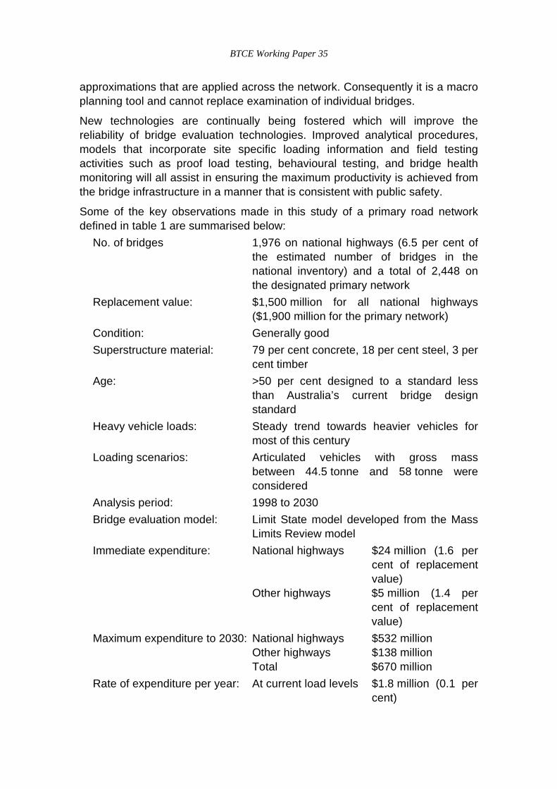
BTCE Working Paper 35
approximations that are applied across the network. Consequently it is a macroplanning tool and cannot replace examination of individual bridges.
New technologies are continually being fostered which will improve thereliability of bridge evaluation technologies. Improved analytical procedures,models that incorporate site specific loading information and field testingactivities such as proof load testing, behavioural testing, and bridge healthmonitoring will all assist in ensuring the maximum productivity is achieved fromthe bridge infrastructure in a manner that is consistent with public safety.
Some of the key observations made in this study of a primary road networkdefined in table 1 are summarised below:
No. of bridges 1,976 on national highways (6.5 per cent ofthe estimated number of bridges in thenational inventory) and a total of 2,448 onthe designated primary network
Replacement value: $1,500 million for all national highways($1,900 million for the primary network)
Condition: Generally good
Superstructure material: 79 per cent concrete, 18 per cent steel, 3 percent timber
Age: >50 per cent designed to a standard lessthan Australia’s current bridge designstandard
Heavy vehicle loads: Steady trend towards heavier vehicles formost of this century
Loading scenarios: Articulated vehicles with gross massbetween 44.5 tonne and 58 tonne wereconsidered
Analysis period: 1998 to 2030
Bridge evaluation model: Limit State model developed from the MassLimits Review model
Immediate expenditure: National highways $24 million (1.6 percent of replacementvalue)
Other highways $5 million (1.4 percent of replacementvalue)
Maximum expenditure to 2030: National highways $532 millionOther highways $138 millionTotal $670 million
Rate of expenditure per year: At current load levels $1.8 million (0.1 percent)

BTCE Working Paper 35
— national highways$2.5 million (0.1 percent)— primary network
At future load levels $26.9 million (1.8 percent) — nationalhighways$36.5 million (1.9 percent) — primarynetwork
This study has been based on approximately 8 per cent of Australia’s bridges.This is the best maintained and strongest group of bridges in the network. Thebridges on the secondary and local roads that feed the primary network aregenerally older and weaker and thus would show much higher replacementrates if the above model was applied across the entire bridge infrastructure.
BIBLIOGRAPHY
AUSTROADS 1992, Bridge Design Code, AUSTROADS, Sydney.
Bureau of Transport and Communication Economics (BTCE) 1994, Adequacyof Transport Infrastructure, in National Planning Transport Task Force Report,Volume 1 Building for the Job, Canberra.
Fry, A T, Easton, G R, Ker, I R, Stevenson, J, and Webber, J R (1976). A Studyof the Economics of Road Vehicle Limits, Report R2, Evaluation andConclusions. National Association of Australian State Road Authorities,Sydney.
Heywood, R.J. (1990), Australian legal limits and relationship to bridge designloads, Proc. 15th Australian Road Research Board Conference, August,Darwin, Australia, Part 3, pp. 209-222.
Heywood R.J. (1993), Bridge Live Load Models from Weigh-in-motion Data,PhD Thesis, University of Queensland, Brisbane, Australia.
Heywood, R.J. (1995a), Live Loads on Australian Bridges—Statistical Modelsfrom Weigh-in-motion Data, Australian Civil Engineering Transactions,Vol. CE37, No. 2, May 1995, pp. 107-116.

BTCE Working Paper 35
Heywood, R.J. (1995b), Live Loads on Australian Bridges—RepresentativeVehicles from Weigh-in-motion Data, Australian Civil Engineering Transactions,Vol. CE37, No. 2, May 1995, pp. 117-126.
Heywood, R.J. (1996), Road Profiles and Bridge Loads, Proc of Asia-Pacificconference on Bridge Loading and Fatigue, Melbourne, 17-18 December.
Heywood, R.J., Ariyaratne, W., Wedgwood, R.J.L. & Oates, R. (1996),Australia’s Bridge Proof Loading Facility - a cost effective asset managementtool, Proceedings of ARRB Transport Research / Transit New ZealandConference, Roads96, Christchurch NZ.
Heywood, R.J., McLean J.R., Ramsay, E.D. & Karagania R.M. (1996), RoadRoughness - Infrastructure Damage Based Standards, Proceedings of ARRBTransport Research / Transit New Zealand Conference, Roads96, ChristchurchNZ.
Heywood, R.J. & McDonnell, A. (1996) Proof Load Testing and Monitoring ofthe South Pine River Bridge, Proc of Asia-Pacific Conference on BridgeLoading and Fatigue, Melbourne, 17-18 December.
Heywood R.J. (1996), Influence of road friendly suspensions on dynamic bridgeloading, Mass Limits Review - Technical Supplement, No 2, National RoadTransport Commission, Melbourne, pp 119-146.
National Association of Australian State Road Authorities (NAASRA) (1970),NAASRA Highway Bridge Design Specification, Sydney, Australia.
National Association of Australian State Road Authorities (NAASRA) (1973),NAASRA Highway Bridge Design Specification (Metric Addendum), Sydney,Australia.
National Association of Australian State Road Authorities (NAASRA) (1976a),NAASRA Bridge Design Specification, Sydney, Australia.
National Association of Australian State Road Authorities (NAASRA) (1976b),Economics of Road Vehicle Limits Study, Report T6, The structural implicationsof the axle spacing/mass schedule, Charrett, Sydney, Australia.
National Association of Australian State Road Authorities (NAASRA) (1985),Axle spacing/mass schedule study Technical Supplement Volume 5, Review ofRoad Vehicle Limits for vehicles using Australian roads, Sydney, Australia.

BTCE Working Paper 35
National Association of Australian State Road Authorities (NAASRA) (1986a),Review of Road Vehicle Limits for Vehicles using Australian Roads, Sydney,Australia.
National Association of Australian State Road Authorities (NAASRA) (1986b),Results of Analyses - Review of Road Vehicle Limits for Vehicles usingAustralian Roads, Technical Supplement Volume 11, Sydney, Australia.
National Association of Australian State Road Authorities (NAASRA) (1987),Draft NAASRA Bridge Design Code, Australia.
National Road Transport Commission (NRTC 1996a). Mass Limits Review -Report and Recommendations of the Steering Committee. National RoadTransport Commission, Melbourne.
National Road Transport Commission (NRTC 1996b). Mass Limits Review,Appendices to Technical Supplement No.2 — Road and Bridge Statistical DataTables. National Road Transport Commission, Melbourne.
Pearson R. A., and Bayley, C. (1997). Economic Impacts of Higher BridgeDesign Loadings; Stage 1, Vehicle alternatives and benefits. Report toAustroads.

BTCE Working Paper 35
ATTACHMENT A MS18 AND T44 BRIDGE DESIGN LOADS
FIGURE A.1 THE USA AND AUSTRALIAN H AND HS SERIES OF BRIDGE DESIGN LIVELOADS AND THEIR M AND MS METRIC EQUIVALENTS.
4.25 m (14 ft) Varies - 4.25 m to 9.15 m (14 ft to 30 ft)
Varies - 9.5 m to 13.4 m (28 ft to 44 ft)
HS20, MS18HS15, MS13.5H20, M18H15, M13.5H10, M9
32,000 lb, 144kN24,000 lb, 108 kN32,000 lb, 144 kN24,000 lb, 108 kN16,000 lb, 72 kN
8,000 lb, 36kN6,000 lb, 27 kN8,000 lb, 36 kN6,000 lb, 27 kN4,000 lb, 18 kN
32,000 lb, 144kN24,000 lb, 108 kN32,000 lb, 144 kNzerozero
(a) Truck loadings
w
P
P w
Design loadingmoment (shear)
[lb]moment (shear)
[kN] [lb/ft] [kN/m]
H20, HS20, M18 & MS18 18 000 (26 000) 80 (116) 640 9.4
H15, HS15, M13.5 & MS13.5 13 500 (19 500) 60 (87) 480 7.0
H10, M9 9 000 (13 000) 40 (58) 320 4.7

BTCE Working Paper 35
(b) Lane loadings
FIGURE A.2 THE AUSTRALIAN T44 LOADING. (1976 TO PRESENT)
48 kN 192 kN
3.7 m 1.2 m Varies - 3.0 m to 8.0 m
Varies - 9.1 m to 14.1 m
1.2 m
192 kN
(a) T44 truck loading
12.5 kN/m
NAASRA 1976106 kN (moment)154 kN (shear)
AUSTROADS 1992150 kN (moment)150 kN (shear)
(b) T44 lane loading
140 kN
(c) A14 standardvehicle loading

BTCE Working Paper 35
ATTACHMENT B BRIDGE REPLACEMENT COSTS
($ per square metre of deck area)
Configuration
Span (m) Steel-Beam-SS Steel-Beam-Cont Steel-Truss Timber-Beam-SS Timber-Truss/arch
<=5 1291 1237 1237 1184 1506
5-7 1291 1237 1237 1184 1506
7-9 1345 1237 1237 1237 1506
9-11 1345 1291 1291 1291 1506
11-13 1399 1291 1291 1345 1506
13-15 1399 1345 1345 1399 1506
15-20 1453 1345 1345 1453 1506
20-30 1506 1399 1399 1506 1506
>30 1937 1829 1829 1829 1829
Unknown - - - - -
Configuration
Span (m)Rconc-Slab-
SS
Rconc-Slab-
Cont Rconc-Beam-SS Rconc-Beam-Cont
Rconc-Box-
SS
Rconc-Box-
Cont
<=5 1076 1022 1076 1022 1184 1130
5-7 1076 1022 1076 1022 1184 1076
7-9 1130 1076 1130 1076 1237 1184
9-11 1130 1076 1130 1076 1237 1184
11-13 1184 1076 1184 1130 1291 1184
13-15 1184 1184 1184 1130 1291 1237
15-20 1184 1237 1237 1237 1234 1291
20-30 1291 1237 1291 1506 1399 1345
>30 1614 1506 1614 1506 1722 1614
Unknown - - - - - -

BTCE Working Paper 35
Configuration
Span (m)Pconc-Slab-SS
Pconc-Slab-Cont
Pconc-Beam-SS
Pconc-Beam-Cont
Pconc-Box-SS
Pconc-Box-Cont Other
<=5 1076 1022 1076 1022 1184 1076 -
5-7 1076 1022 1076 1022 1184 1076 -
7-9 1130 1076 1130 1076 1237 1130 -
9-11 1130 1076 1130 1076 1237 1130 -
11-13 1184 1130 1184 1130 1291 1184 -
13-15 1184 1130 1184 1130 1291 1184 -
15-20 1237 1237 1237 1184 1345 1291 -
20-30 1291 1506 1291 1237 1399 1345 -
>30 1614 1506 1614 1506 1722 1668 -
Unknown - - - - - - -

BTCE Working Paper 35
APPENDIX V COMMENTS BY STATE AND TERRITORYROAD AUTHORITIES
States and territories were invited by the BTCE to comment on the BTCE’smethodology and results. This appendix contains all responses received at thetime of printing. Responses have not been edited.
These comments are available from the BTCE upon request.

BTCE Working Paper 35
APPENDIX VI BTCE RESPONSE TO COMMENTS FROMSTATES AND TERRITORIES IN APPENDIX V
The BTCE again acknowledges with gratitude the cooperation of the variousjurisdictions in providing data and comment in the modelling exerciseundertaken to provide input to the Committee of Inquiry into Federal RoadFunding.
The draft provided to the States and Territories on 26 September did notinclude final results for some jurisdictions because not all the necessary datawere available to the BTCE at the time. While this was unavoidable, it mayhave disadvantaged those states in providing considered comment to theBTCE.
Rather than addressing all the points made by individual jurisdictions, only anumber of the more substantive issues raised have been addressed belowunder generic headings. Factual errors made by some jurisdictions in theircomments have been ignored in the interests of maintaining discussion onconcrete issues.
COST ESTIMATES USED BY THE BTCE
Some jurisdictions considered BTCE estimates of unit and total costs for areassuch as maintenance to be too low. Others held the opposite view. Differenceswere also apparent on the issue of desirable frequency of resealing of roadpavement, and hence the figure used in the BTCE model.
These differences highlight different conditions due to Australian geography, aswell as differences in maintenance practices by the various road authorities.The BTCE considers that the use of averaged cost and other data is notdesirable because it cannot provide accurate estimates of overall expenditureneeds, and may disadvantage some jurisdictions (while advantaging others). Ifresources and data were to become available, this aspect of the modellingcould easily be rectified.

BTCE Working Paper 35
STRATEGIC NATURE OF BTCE MODEL
A related issue is the ‘strategic’ nature of the output. The BTCE agrees that itsoutput cannot provide a guide to specific projects. Indeed, it is not intended todo so. Its purpose is to identify sections of road that warrant more detailed cost-benefit analysis by individual road authorities which have local expertise. TheBTCE modelling also provides indicative figures for road expenditure requiredin the future to assist in budgetary planning.
ROUGHNESS INTERVENTION LEVELS
Following advice from ARRB Transport Research Ltd., a maximum roughnessconstraint of 160 NRM was imposed in the model. However, most interventionlevels derived by the BTCE model are well below this figure.
FLOODING, TOWN BYPASSES, BRIDGES AND ROADTRAINS
The BTCE acknowledges fully in several parts of its study that further work isrequired on flood mitigation works, town bypasses, bridge needs if mass limitsare increased, and roadtrain requirements. Apart from resource issues in termsof BTCE capability, however, it is also necessary to bear in mind that credibleestimates in these areas would require provision by the jurisdictions of highlydetailed data.
Rigorous cost-benefit analysis would be required before any estimates weremade and published by the BTCE. In some instances, preliminary work by theBTCE suggests that estimated expenditure needs may not be significant,particularly when compared with other modelling and data uncertainties.
FORECASTS OF ROAD USAGE
A number of jurisdictions have commented on the simplicity of using anassumption that freight traffic will grow by 3 per cent per annum. The BTCEendorses this position.
However, cost-benefit modelling of road infrastructure requires forecasts oftraffic growth for individual sections of each road. While most jurisdictions areable to provide global estimates of freight growth (presumably based onforecasts of economic growth in the state or territory), the BTCE did not haveavailable to it the more detailed figures required to carry out its analysis on anationally consistent basis.
ROADS ANALYSED
A meeting of State and Territory officials with the BTCE in Canberra on19 August agreed that the BTCE should analyse roads identified in 1996 as

BTCE Working Paper 35
being of national importance by a working party (Infrastructure and PolicyPlanning, IAPP) established under the aegis of the Australian TransportCouncil. However, the BTCE was not able to obtain from the IAPP Secretariat alist of the roads that its members had identified, and did not have the time orresources to draw up a list itself from a map supplied by the IAPP Secretariat.
The BTCE itself makes no judgement on which non-NHS roads are of nationalsignificance.
CONCLUSION
The BTCE is committed to transparency in its research. It has thereforeacknowledged above and elsewhere a number of the qualifications identified bythe States and Territories. We again stress that the strategic character of themodelling means that figures for individual sections of road should be regardedas indicative, not conclusive.
1 October 1997

BUREAU OF TRANSPORT AND COMMUNICATIONS ECONOMICS
RECENT PUBLICATIONS
REPORTS
92 Traffic congestion and road user charges in Australian capital cities (1996) $14.95 (96 0260 7)
93 Australian commercial television 1986–1995: Structure and performance (1996) $19.95 (96 0403 0)
94 Transport and greenhouse: Costs and options for reducing emissions (1996) $54.95 (96 0691 2)
95 General aviation flying in Australia (1996) $24.95 (96 0691 2)
96 Transport and greenhouse: Costs and options for reducung emissions (1996) $54.95 (96 0630 0)
97 Quality of rail service: The customer’s perspective (1997) $11.95 (96 1017 0)
OCCASIONAL PAPERS
111 Residential demand for access to broadband services: An empirical investigation (1996) $16.95 (96 0185 6)
112 Film and television co-production in Australia (1996) (Free from the BTCE)
113 Measuring community benefits of Australian TV programs (1996) $14.95 (96 0016 7)
WORKING PAPERS (Free from the BTCE)
30 Interconnection pricing principles (1997)
31 Australian content on pay TV (1997)
32 Roads, vehicle performance and greenhouse: Costs and emission benefitsof smoother highways (1997)
33 Benefits of private sector involvement in road provision: A look at the evidence(1997)
34 Taxes and charges in Australian transport: A transmodal overview (1997)
BULLETINS (Free from the BTCE)
Transport and Communications Indicators (Quarterly)
Waterline (Quarterly)
Research in Communication Economics in Australia Bulletin 3 (1996)
INTERNET
http://www.dot.gov.au/programs/btce/btcehome.htm
To order free publications write to the BTCE, GPO Box 501, Canberra ACT 2601, Australia, telephone 02 6274 6846,or email [email protected]. Other titles are on sale from the Australian Government Publishing Service, GPO Box 84,Canberra ACT 2601, Australia, telephone 02 6295 4861 (AGPS catalogue number is in brackets).