w o r k i n g

p a p e r

F E D E R A L R E S E R V E B A N K O F C L E V E L A N D

18 03

Assessing International Commonality in Macroeconomic Uncertainty and Its Effects

Andrea Carriero, Todd E. Clark, and Massimiliano Marcellino

ISSN: 2573-7953

Working papers of the Federal Reserve Bank of Cleveland are preliminary materials circulated to stimulate discussion and critical comment on research in progress. They may not have been subject to the formal editorial review accorded offi cial Federal Reserve Bank of Cleveland publications. The views stated herein are those of the authors and are not necessarily those of the Federal Reserve Bank of Cleveland or the Board of Governors of the Federal Reserve System.

Working papers are available on the Cleveland Fed’s website: https://clevelandfed.org/wp

Working Paper 18-03 March 2018

Assessing International Commonality in Macroeconomic Uncertainty and Its Effects

Andrea Carriero, Todd E. Clark, and Massimiliano Marcellino

This paper uses a large vector autoregression (VAR) to measure international macroeconomic uncertainty and its effects on major economies, using two datasets, one with GDP growth rates for 19 industrialized countries and the other with a larger set of macroeconomic indicators for the U.S., euro area, and U.K. Using basic factor model diagnostics, we fi rst provide evidence of signifi cant commonality in international macroeconomic volatility, with one common factor accounting for strong comovement across economies and variables. We then turn to measuring uncertainty and its effects with a large VAR in which the error volatilities evolve over time according to a factor structure. The volatility of each variable in the system refl ects time-varying common (global) components and idiosyncratic components. In this model, global uncertainty is allowed to contemporaneously affect the macroeconomies of the included nations—both the levels and volatilities of the included variables. In this setup, uncertainty and its effects are estimated in a single step within the same model. Our estimates yield new measures of international macroeconomic uncertainty, and indicate that uncertainty shocks (surprise increases) lower GDP and many of its components, adversely affect labor market conditions, lower stock prices, and in some economies lead to an easing of monetary policy.

Keywords: Business cycle uncertainty, stochastic volatility, large datasets.

J.E.L. Classifi cation: F44, E32, C55, C11.

Suggested citation: Carriero, Andrea, Todd E. Clark, and Massimiliano Marcellino, 2018. “Assessing International Commonality in Macroeconomic Uncertainty and Its Effects.” Federal Reserve Bank of Cleveland, Working Paper no. 18-03.https://doi.org/10.26509/frbc-wp-201803.

Andrea Carriero is at Queen Mary, University of London, Todd E. Clark (cor-responding author) is at the Federal Reserve Bank of Cleveland (todd.clark@re-searchfed.org), and Massimiliano Marcellino is at Bocconi University, IGIER, and CEPR. The authors gratefully acknowledge research assistance from John Zito and helpful comments from Efrem Castelnuovo. Carriero gratefully acknowledges support for this work from the Economic and Social Research Council [ES/K010611/1].

1 Introduction

Since the seminal analysis of Bloom (2009), a large body of research has examined the mea-

surement of macroeconomic uncertainty and its effects on the economy. Bloom (2014) surveys

related work up through several years ago. Additional recent contributions include Baker,

Bloom and Davis (2016), Basu and Bundick (2017), Caggiano, Castelnuovo, and Groshenny

(2014), Carriero, Clark, and Marcellino (2017, 2018), Gilchrist, Sim, and Zakrajsek (2014),

Jo and Sekkel (2017), Jurado, Ludvigson, and Ng (2015), Leduc and Liu (2016), Ludvigson,

Ma, and Ng (2016), and Shin and Zhong (2016).

Although much of the literature has focused on uncertainty within a single economy, some

work has examined common international aspects of uncertainty and its effects. Theoretical

studies include Gourio, Siemer, and Verdelhan (2013) and Mumtaz and Theodoridis (2017).

The former develops an international real business cycle model in which an increase in

the probability of disaster leads to a decline in GDP, investment, and employment, with

larger effects on the economy that would be more affected by the disaster. The latter study

builds a two-economy, dynamic stochastic general equilibrium model to explain evidence of

international comovement in volatilities, in a framework where cross-country risk sharing (for

consumption smoothing) and trade openness help to drive such comovement of volatilities.

A larger set of studies has assessed empirical evidence of common international aspects

of uncertainty and its effects. These studies have relied on a variety of models or methods,

to assess sometimes different questions. In a dataset of 243 variables for 11 industrialized

countries, Mumtaz and Theodoridis (2017) apply a factor model with stochastic volatility

components common to the world and each country. They find the global component to be

an important driver of time-varying volatility. Using GDP growth for 20 countries, Berger,

Grabert, and Kempa (2016) estimate a factor model with stochastic volatility components

common to the world and specific to each country; in a second step, for each country,

they estimate vector autoregressions (VARs) with other variables and uncertainty to assess

the effects of uncertainty. Carriere-Swallow and Cespedes (2013) and Gourio, Siemer, and

Verdelhan (2013) also use simple, small VAR approaches, measuring uncertainty with the

volatility of stock returns. One finding of note in Carriere-Swallow and Cespedes (2013)

is that responses to uncertainty shocks differ for developed economies and emerging mar-

ket economies, with larger and more persistent effects on investment and consumption for

emerging markets. Using 45 variables for G-7 nations, Cuaresma, Huber, and Onorante

1

(2017) apply a VAR with common factors in shocks that have a time-varying variance repre-

sented with stochastic volatility. Their estimates yield a common uncertainty factor that is

closely tied to the volatility of global equity prices, and shocks to that factor have significant

macroeconomic and financial effects.

Some other analyses have assessed international comovement in financial uncertainty.

Using data on realized stock return volatility and GDP growth in 33 countries, Cesa-Bianchi,

Pesaran, and Rebucci (2017) show that return volatility is much more correlated across

countries than is GDP growth, that global growth has a sizable contemporaneous impact on

financial volatility, and that a common factor accounts for the bulk of the correlation between

return volatility and growth. Casarin, Foroni, Marcellino, and Ravazzolo (2017) propose

a Bayesian panel model for mixed frequency data, with random effects and parameters

changing over time according to a Markov process, to study the effects of macroeconomic

and financial uncertainty on a set of 11 macroeconomic variables per country, for a set

of countries including the U.S., several European countries, and Japan. In their analysis,

macroeconomic uncertainty is measured by the cross-sectional dispersion in survey forecasts

of GDP growth, and financial uncertainty is measured by the VIX for the U.S. They find

that, for most of the variables, financial uncertainty dominates macroeconomic uncertainty,

and the effects of uncertainty differ depending on whether the economy is in a contraction

or expansion regime.

Extending this prior work, in this paper we use large Bayesian VARs (BVARs) to measure

international macroeconomic uncertainty and its effects on major economies. We do so for

two datasets, one consisting of GDP growth for 19 industrialized economies and the other

comprising of 67 variables in quarterly data for the U.S., euro area (E.A.), and U.K. from

the mid-1980s through 2013. We first use the basic factor model diagnostics surveyed in

Stock and Watson (2016) to assess the common factor structure of the stochastic volatilities

of BVARs. Then, to estimate global uncertainty and its effects, we turn to our preferred

large, heteroskedastic VAR in which the error volatilities evolve over time according to a

factor structure, as developed in the U.S.-only analysis of Carriero, Clark, and Marcellino

(2017). The volatility of each variable in the system reflects time-varying common (global)

components and idiosyncratic components. In this model, global uncertainty is allowed to

contemporaneously affect the macroeconomies of the included nations — both the levels and

volatilities of the included variables. Changes in the common components of the volatilities

2

of the VAR’s variables provide contemporaneous, identifying information on uncertainty. In

this setup, uncertainty and its effects are estimated in a single step within the same model.

Our results point to significant commonality in international macroeconomic volatility,

with one common factor — our measure of global uncertainty — accounting for strong co-

movement across economies and variables in each of our datasets. Our global uncertainty

measure is strongly correlated with a comparable measure for the U.S. from Carriero, Clark,

and Marcellino (2017) and to a modestly lesser extent with the Jurado, Ludvigson, and

Ng (2015) estimate of U.S. macroeconomic uncertainty. This suggests that global macroe-

conomic uncertainty is closely related to uncertainty in the U.S., which might not seem

surprising given the tie of the international economy to the U.S. economy. Our estimate of

global macroeconomic uncertainty appears to be more modestly correlated with estimates of

financial uncertainty from the literature and the global economic policy uncertainty measure

of Davis (2016).

Our results also include impulse response functions for a surprise increase in global

macroeconomic uncertainty. According to these estimates, a shock to global uncertainty

reduces GDP in most industrialized countries. In the larger set of indicators for the U.S.,

E.A., and U.K., the surprise increase in uncertainty lowers GDP and many of its compo-

nents, adversely affects labor market conditions, lowers stock prices, and in some economies

leads to an easing of monetary policy. Our identified global uncertainty shock is uncorrelated

with other structural (U.S.-based) shocks, such as productivity, fiscal, or monetary shocks.

Hence, the responses are capturing a genuine effect from unexpected increases in uncertainty.

Historical decomposition estimates for the 19-country GDP dataset indicate that, while

shocks to uncertainty can have noticeable effects on GDP growth in many countries, on bal-

ance they are not a primary driver of fluctuations in macroeconomic and financial variables.

For example, over the period of the Great Recession and subsequent recovery, shocks to

uncertainty made modest contributions to the paths of GDP growth in many countries (e.g.,

U.S., France, Spain, and Sweden) and small contributions in some countries (e.g., Japan and

Norway). In the declines of GDP growth observed in a number of countries in the early 1990s

and early 2000s, uncertainty shocks made small contributions in some countries (e.g., U.S.,

Sweden, and U.K.). Overall, shocks to the VAR’s variables played a much larger role than

did uncertainty shocks. However, there is a sense in which that is a natural result of con-

sidering the VAR shocks jointly as a set versus the uncertainty shock by itself; individually,

3

some or many of the VAR shocks would also play small or modest roles.

We should also mention that, naturally, there is imprecision around both estimated un-

certainty and its effects, with the extent of the imprecision generally underestimated when

simpler econometric methods than ours are employed. Actually, our methodology allows

us to avoid some of the limitations of previous empirical studies of the effects of interna-

tional macroeconomic uncertainty (second moments) on macroeconomic fluctuations (first

moments). The analysis of Mumtaz and Theodoridis (2017) is focused on international com-

ponents of second moments. The model of Cuaresma, Huber, and Onorante (2017) may

confound first-moment shocks with second-moment changes by imposing not only a common

element of shock variances but also the same common element of shocks. In addition, in

their setup, second-moment changes do not have direct effects on the levels of variables. The

analysis of Berger, Grabert, and Kempa (2016) relies on a two-step approach common in

the uncertainty literature, in which a measure of uncertainty is estimated in a preliminary

step and then used as if it were observable data in the subsequent econometric analysis of

its impact on macroeconomic variables. However, as described in Carriero, Clark, and Mar-

cellino (2017), with such a two-step approach, it is possible that measurement error in the

uncertainty estimate could lead to endogeneity bias in estimates of uncertainty’s effects, and

the uncertainty around the uncertainty estimates is not easily accounted for in such a setup,

since the proxy for uncertainty is treated as data. Moreover, the models used in the first

and second steps are somewhat contradictory, with the first step treating second moments

as time-varying and the second treating them as constant over time.

Finally, in the studies that have assessed the effects of uncertainty on macroeconomic

fluctuations across countries, uncertainty has commonly been measured and assessed using

a small set of variables for each country. Other work in the literature, including Jurado,

Ludvigson, and Ng (2015) and Carriero, Clark, and Marcellino (2017), has emphasized some

benefits to using relatively large cross sections. In particular, the use of small VAR models

to assess the effects of uncertainty can make the results subject to the common omitted

variable bias and nonfundamentalness of the errors, and it can assess uncertainty’s impacts

on only a small number of economic indicators.

The paper is structured as follows. Section 2 describes the data. After presenting the

BVAR model with stochastic volatility, Section 3 uses basic factor model diagnostics to

assess the global factor structure in macroeconomic uncertainty. Section 4 introduces our

4

preferred large BVAR model for measuring uncertainty and its effects and then presents

results. Section 5 describes robustness checks. Section 6 summarizes our main findings and

concludes. The appendix details the estimation algorithm.

2 Data

As indicated above, to assess international comovement in uncertainty and the macroeco-

nomic effects of global uncertainty, we rely on two datasets, one consisting of GDP growth

rates for a relatively large set of industrialized economies and the other consisting of a larger

set of macroeconomic variables for three large economies. Although the first dataset is sim-

ilar to others in the literature and helps to establish an international factor structure to

uncertainty, our greater interest is in the second dataset. As noted above, for measuring

uncertainty we believe it preferable to include relatively large variable sets with long time

series.

More specifically, for the GDP growth analysis, we use quarterly data (quarter-on-

quarter rates) in the following 19 industrialized economies, obtained from the OECD’s online

database (OECD 2017): United States, Australia, Austria, Belgium, Canada, Denmark, Fin-

land, France, Germany, Italy, Japan, Luxembourg, Netherlands, Norway, Portugal, Spain,

Sweden, Switzerland, and United Kingdom. For simplicity, in the remainder of the paper

we will refer to this dataset as the 19-country GDP dataset. For the analysis of a wider

set of macroeconomic indicators across industrialized economies, long time series on large

variable sets are difficult to find. Accordingly, we focus on a few major economies for which

relatively large sets of long time series are available: the U.S., euro area, and U.K. For the

U.S. and euro area, we obtain quarterly data on major macroeconomic indicators from the

files of Jarocinski and Mackowiak (2017). After omitting their series with missing data and

a few others (for various reasons, including overlap with other series), we use 51 variables

from their dataset, 26 for the U.S. and the remainder for the E.A. For the U.K., we ob-

tained comparable data on 16 variables from Haver Analytics. Table 1 lists the variables

and any transformations used to achieve stationarity of the data. We will refer to this as

the 3-economy macroeconomic dataset.

In our primary results, the estimation sample starts in 1985, reflecting the availability of

some of the series in the 3-economy macroeconomic dataset. The estimation sample ends in

2016:Q3 for results based on GDP growth for 19 countries and in 2013:Q3 for results with the

5

3-economy macroeconomic dataset (reflecting the span of the Jarocinski-Mackowiak dataset).

In the 19-country GDP dataset, we also consider a sample starting in 1960; the robustness

section describes these results. Following common practice in the factor model literature

as well as studies such as Jurado, Ludvigson, and Ng (2015) and Carriero, Clark, and

Marcellino (2017), after transforming each series for stationarity as needed, we standardize

the data (demean and divide by the simple standard deviation) before estimating the model.

3 Commonality in International Macroeconomic Un-

certainty

To assess the global factor structure of macroeconomic uncertainty, we use the basic factor

model diagnostics surveyed in Stock and Watson (2016) to assess the common factor structure

of the stochastic volatilities of BVARs. We do so for both the 19-country GDP dataset and

the 3-economy macroeconomic dataset. In this section, we first present the BVAR model

with stochastic volatility and then present the factor assessment results.

3.1 BVAR-SV Model

The conventional BVAR with stochastic volatility, referred to as a BVAR-SV specification,

takes the following form, for the n× 1 data vector yt:

yt =

p∑i=1

Πiyt−i + vt

vt = A−1Λ0.5t εt, εt ∼ N(0, In), Λt ≡ diag(λ1,t, . . . , λn,t) (1)

ln(λi,t) = γ0,i + γ1,i ln(λi,t−1) + νi,t, i = 1, . . . , n

νt ≡ (ν1,t, ν2,t, . . . , νn,t)′ ∼ N(0,Φ),

where A is a lower triangular matrix with ones on the diagonal and non-zero coefficients below

the diagonal, and the diagonal matrix Λt contains the time-varying variances of conditionally

Gaussian shocks. This model implies that the reduced-form variance-covariance matrix of

innovations to the VAR is var(vt) ≡ Σt = A−1ΛtA−1′. Note that, as in Primiceri’s (2005)

implementation, innovations to log volatility are allowed to be correlated across variables; Φ

is not restricted to be diagonal. For notational simplicity, let Π denote the collection of the

VAR’s coefficients. Note also that, to speed computation, we estimate the model with the

triangularization approach developed in Carriero, Clark, and Marcellino (2016b). Estimates

6

derived from the BVAR-SV model are based on samples of 5,000 retained draws, obtained

by sampling a total of 30,000 draws, discarding the first 5,000, and retaining every 5th draw

of the post-burn sample.

Regarding the priors for the BVAR-SV model, we set them to generally align with those

of the baseline model with factor volatility detailed in section 4. For the VAR coefficients

contained in Π, we use a Minnesota-type prior. With the variables of interest transformed

for stationarity, we set the prior mean of all the VAR coefficients to 0. We make the prior

variance-covariance matrix ΩΠ diagonal. For lag l of variable j in equation i, the prior

variance is θ21l2

for i = j and θ21θ22

l2σ2i

σ2j

otherwise. In line with common settings for large models,

we set overall shrinkage θ1 = 0.1 and cross-variable shrinkage θ2 = 0.5.1 Consistent with

common settings, the scale parameters σ2i take the values of residual variances from AR(p)

models fit over the estimation sample.

For each row aj of the matrix A, we follow Cogley and Sargent (2005) and make the

prior fairly uninformative, with prior means of 0 and variances of 10 for all coefficients.

The variance of 10 is large enough for this prior to be considered uninformative. For the

coefficients (γi,0, γi,1) (intercept, slope) of the log volatility process of equation i, i = 1, . . . , n,

the prior mean is (0.05 × lnσ2i , 0.95), where σ2

i is the residual variance of an AR(p) model

over the estimation sample; this prior implies the mean level of volatility is lnσ2i . The prior

standard deviations (assuming 0 covariance) are (20.5, 0.3). For the variance matrix Φ of

innovations to log volatility, we use an inverse Wishart prior with mean of 0.03 × In and

n+2 degrees of freedom. For the period 0 values of lnλt, we set the prior mean and variance

at ln σ2i and 2.0, respectively.

3.2 Factor Structure Evidence

Beginning with commonality in uncertainty, Table 2 reports summary statistics on the factor

structure of volatility estimates, relying on the main statistics described and used in the

applications of Stock and Watson (2016). For consistency with the BVAR model with factor

volatility we will consider below, in these factor structure results we measure volatilities

by the posterior medians of lnλi,t. For up through five principal components, we report

the marginal R2 of volatility factors estimated by principal components and the Ahn and

Horenstein (2013) eigenvalue ratio.

1Carriero, Clark, and Marcellino (2015) find little gain from optimal determination of these parameters.

7

For GDP growth in 19 countries, the measures of factor structure suggest one strong

factor in the international volatility of the business cycle as captured by GDP. The first

factor accounts for an average of about 79 percent of the variation in volatility. The second

and third factors account for about 11 and 6 percent, respectively. The Ahn-Horenstein ratio

peaks at one factor with a value of 7.4, compared to 1.7 and 3.0 for the second and third

factors, respectively. As reported in Table 3, the factor loadings associated with the principal

components are fairly tightly clustered around 1, with a minimum of 0.751 for Denmark and

a maximum of 1.114 for Sweden.

For the larger set of macroeconomic indicators for the U.S., E.A, and U.K., we use

volatility estimates from BVAR-SV models fit for each economy to assess the degree of

commonality — and factor structure — in volatility.2 Figure 1 compares volatility estimates

across these three economies for a subset of major macroeconomic indicators (we use a

subset to limit the number of charts). In this comparison, volatility is reported in the way

common in the literature, as the (posterior median of the) standard deviation of the reduced-

form innovation in the BVAR, given by the square root of the diagonal elements of Σt.

Qualitatively, these estimates suggest considerable commonality within and across countries.

As the chart indicates, for a given country, there is significant comovement across variables.

For example, for the U.S., most variables display a rise in volatility around the recessions of

the early 1990s, 2001, and 2007-2009. For the E.A., most variables display sizable increases

in uncertainty in the early and mid-1990s and again with the Great Recession. In addition,

there appears to be significant comovement across economies, somewhat more so for volatility

in the U.S. and E.A. than in the case of the U.K.

To more formally assess commonality in volatility in the 3-economy macroeconomic

dataset, the last two columns of Table 2 report summary statistics on the factor struc-

ture of volatility estimates across countries and variables. Again, for consistency with the

BVAR model with factor volatility we will consider below, in these factor structure results

we measure volatilities by the posterior medians of lnλi,t. Although we omit the results in

the interest of brevity, to distinguish possible dynamic versus static factors, we have applied

the same analysis to the posterior medians of the shocks to lnλi,t obtained in the BVAR-SV

estimation. We have also applied the factor analysis metrics to the reduced-form volatilities

2We estimate the model separately for each country rather than as one single system to avoid an undulyinformative proper prior on the log volatility innovation variance matrix Φ. With 67 variables in a jointsystem, a proper inverse Wishart prior on Φ would be very informative in the context of an estimationsample of fewer than 150 observations.

8

given by the (posterior median of the) square root of the diagonal elements of Σt. In both

cases, we obtained results similar to those reported for the lnλi,t estimates.

As indicated in Table 2, for the 3-economy macroeconomic dataset, a first factor accounts

for an average of about 42 percent of the variation in volatility. By comparison, the role

of the first factor in volatility is much stronger in this dataset (and in the 19-country GDP

dataset) than in the monthly U.S. data of Jurado, Ludvigson, and Ng (2015). Their sup-

plemental appendix notes that a first factor accounts for an average of about 11 percent of

the variation in volatility in their large dataset. In our estimates, for most variables, the

estimated loadings on this factor reported in Table 4 are clustered around a value of 1. For

example, the loadings on GDP growth are 1.330 for the U.S., 1.288 for the E.A., and 1.188

for the U.K. Overall, the patterns in the estimated factor loadings appear consistent with an

interpretation in which the first factor is capturing a common component in macroeconomic

volatilities, with most loadings clustered around values of 1, most prominently for the U.S.

variables, almost as clearly for the E.A., and with modestly more dispersion in loadings on

the U.K. variables. A second factor accounts for about 26 percent of the variation in inter-

national macroeconomic volatility. Together, two factors account for more than 68 percent

of the variation in volatility across macroeconomic indicators and countries. Subsequent fac-

tors account for significantly smaller marginal shares of variation. The Ahn-Horenstein ratio

peaks at two factors. Together, the R2 and Ahn-Horenstein estimates suggest two factors in

this larger dataset.

4 Measuring the Impact of Uncertainty

Having established evidence of common factors in international macroeconomic volatilities,

we now turn to assessing the effects of global uncertainty on macroeconomic fluctuations.

This section begins by detailing the Bayesian VAR with a generalized factor structure

(BVAR-GFSV) we use for that purpose, first for a one-factor model we use with the 19-

country GDP dataset and then for a two-factor specification we use with 3-economy macroe-

conomic dataset. We then present results for the uncertainty estimates and effects of shocks

to uncertainty. Readers not interested in technical details can go directly to the results in

section 4.4.

9

4.1 One-Factor BVAR-GFSV Model

With the evidence in the previous section pointing to one factor in the 19-country GDP

dataset, we rely on a one-factor model in our baseline results for the dataset.

Let yt denote the n × 1 vector of variables of interest — covering multiple countries —

and vt denote the corresponding n× 1 vector of reduced-form shocks to these variables. The

reduced-form shocks are:

vt = A−1Λ0.5t εt, εt ∼ iid N(0, I), (2)

where A is an n × n lower triangular matrix with ones on the main diagonal, and Λt is a

diagonal matrix of volatilities, λi,t, i = 1, . . . , n. For each variable i, its log-volatility follows a

linear factor model with a common uncertainty factor lnmt that follows an AR(pm) process

augmented to include yt−1 and an idiosyncratic component lnhi,t that follows an AR(1)

process:

lnλi,t = βm,i lnmt + lnhi,t, i = 1, . . . , n (3)

lnmt =

pm∑i=1

δm,i lnmt−i + δ′m,yyt−1 + um,t, um,t ∼ iid N(0, φm) (4)

lnhi,t = γi,0 + γi,1 lnhi,t−1 + ei,t, i = 1, . . . , n. (5)

The volatility factor mt is our measure of (unobservable) global macroeconomic uncertainty.

Note that the uncertainty shock um,t is independent of the conditional errors εt, and νt =

(e1,t, ..., en,t)′ jointly distributed as i.i.d. N(0,Φν) and independent among themselves, so

that Φν = diag(φ1, ..., φn). For identification, we follow common practice in the dynamic

factor model literature (e.g., Otrok and Whiteman 1998) and assume lnmt to have a zero

unconditional mean, fix the variance φm at 0.03, and use a simple accept-reject step to

restrict the first variable’s (U.S. GDP growth) loading to be positive.

The global uncertainty measure mt can also affect the levels of the macroeconomic vari-

ables contained in yt, contemporaneously and with lags. In particular, yt is assumed to

follow:

yt =

p∑i=1

Πiyt−i +

pm∑i=0

Πm,i lnmt−i+1 + vt, (6)

where p denotes the number of yt lags in the VAR, pm denotes the number of lnmt lags in

the conditional mean of the VAR (deliberately set, for computational convenience, to the lag

order of the factor process), Πi is an n × n matrix, i = 1, ..., p, and Πm,i is an n × 1 vector

of coefficients, i = 0, ..., pm.

10

This model allows the international business cycle to respond to movements in global

uncertainty, both through the conditional variances (contemporaneously, via movements in

vt) and through the conditional means (contemporaneously and with lag, via the coefficients

collected in Πm,i, i = 0, ..., pm. In our implementation, we set the model’s lag orders at p = 2

and pm = 2. Note that yt cannot contemporaneously affect uncertainty, which in this sense is

treated as exogenous. (However, it is not entirely exogenous: The model allows uncertainty

to respond with a lag to macroeconomic conditions.) Carriero, Clark, and Marcellino (2018)

develop a model with endogenous uncertainty, but empirically they find little evidence of

contemporaneous effects of yt on macroeconomic uncertainty for the U.S.

4.2 Two-Factor BVAR-GFSV Model

With Section 2’s principal component-based analysis of volatilities obtained from BVAR-

SV estimates pointing to two factors in the 3-economy macroeconomic dataset, we consider

specifications with two common volatility components. The natural starting point would be

the model described above extended to include a second factor in both the volatility process

and the VAR’s conditional mean. In unreported estimates, we considered such a model,

as well as a one-factor model. The estimate of the first factor in this unrestricted two-

factor specification was very similar to the estimate obtained from a one-factor specification

and strongly correlated with the first principal component of BVAR-SV volatilities. The

estimated second factor seemed to capture (with considerable variability in the estimate

from quarter to quarter) a modest low-frequency decline in volatility from the first half

of the sample to the second half, with generally insignificant effects on the levels of the

variables. However, these results from an unrestricted two-factor specification appear to

suffer problems with the convergence of the Markov Chain Monte Carlo (MCMC) sampler

with this dataset (although not with other datasets).

From this analysis, we conclude that although there are two volatility or uncertainty

factors in the 3-economy macroeconomic dataset, only one bears on the levels of macroeco-

nomic variables. As we describe in more detail in the robustness section below, we obtained

a qualitatively similar result with an alternative simple approach of adding to the macroe-

conomic BVAR the principal components of the BVAR-SV volatilities used in this section

(an approach common in the uncertainty literature, as in, e.g., Jurado, Ludvigson, and Ng

2015, though suboptimal as it ignores that uncertainty is a generated regressor).

11

Accordingly, for the 3-economy macroeconomic dataset, our baseline results use a two-

factor model with some restrictions. In particular, the model features two common factors

in volatilities but includes only one of the factors in the conditional mean of the VAR and

affecting the levels of the included variables. In addition, reflecting other evidence, the

idiosyncratic component of volatility is simply a constant. With the larger set of indicators

for the U.S., E.A., and U.K. in our sample of quarterly data starting in the 1980s, unreported

estimates of a version of the model with an AR(1) process for the idiosyncratic component of

volatility — a specification that yields results very similar to those we report — display very

little time variation in the idiosyncratic components. For the 3-economy macroeconomic

dataset, our model estimates attribute the vast majority of time variation in volatility to the

common component mt.

With these restrictions, the model applied to the 3-economy macroeconomic dataset takes

the following form, including two international uncertainty factors mt and ft:

yt =

p∑i=1

Πiyt−i +

pm∑i=0

Πm,i lnmt−i+1 + vt (7)

vt = A−1Λ0.5t εt, εt ∼ iid N(0, I) (8)

lnλi,t = βm,i lnmt + βf,i ln ft + lnhi, i = 1, . . . , n (9)

lnmt =

pm∑i=1

δm,i lnmt−i + δ′m,yyt−1 + um,t, um,t ∼ iid N(0, φm) (10)

ln ft =

pf∑i=1

δf,i ln ft−i + δ′f,yyt−1 + uf,t, uf,t ∼ iid N(0, φf ). (11)

In this case, the log-volatility of each variable i follows a linear factor model with common

unobervable uncertainty factors lnmt and ln ft, which follow independent AR processes aug-

mented to include yt−1, and a constant idiosyncratic component lnhi. The volatility factors

mt and ft are measures of (unobservable) global macroeconomic uncertainty. However, only

the first global uncertainty measure, mt, enters the conditional mean of the VAR and affects

the levels of the macroeconomic variables contained in yt, contemporaneously and with lags.

To spell out the notation, which follows that used in the one-factor model above, A is

an n × n lower triangular matrix with ones on the main diagonal; Λt is a diagonal matrix

of volatilities, λi,t, i = 1, . . . , n; p denotes the number of yt lags in the VAR; pm denotes the

number of lnmt lags in the conditional mean of the VAR; Πi is an n× n matrix, i = 1, ..., p;

and Πm,i is an n× 1 vector of coefficients, i = 0, ..., pm. The uncertainty shocks um,t and uf,t

12

are independent of each other and independent of the conditional errors εt. For identification,

we assume that lnmt and ln ft have zero unconditional means, fix their variances φm and

φf at 0.03, and use a simple accept-reject step to restrict the first factor’s loading on U.S.

GDP growth and the second factor’s loading on E.A. GDP growth to be positive. In our

implementation, we set the model’s lag orders at p = 2, pm = 2, and pf = 2.

4.3 Priors and Estimation

For the VAR coefficients contained in Π, we use a Minnesota-type prior. With the variables

of interest transformed for stationarity, we set the prior mean of all the VAR coefficients to

0. We make the prior variance-covariance matrix ΩΠ diagonal. The variances are specified

to make the prior on the lnmt terms fairly loose and the prior on the lags of yt take a

Minnesota-type form. Specifically, for the lnmt terms of equation i, the prior variance is

θ23σ

2i . For lag l of variable j in equation i, the prior variance is θ21

l2for i = j and θ21θ

22

l2σ2i

σ2j

otherwise. In line with common settings, we set overall shrinkage θ1 = 0.1 and cross-variable

shrinkage θ2 = 0.5; we set factor coefficient shrinkage θ3 = 10. Finally, consistent with

common settings, the scale parameters σ2i take the values of residual variances from AR(p)

models fit over the estimation sample.

Regarding priors attached to the volatility-related components of the model, for the

rows aj of the matrix A, we follow Cogley and Sargent (2005) and make the prior fairly

uninformative, with prior means of 0 and variances of 10 for all coefficients.

For the loading βi,m, i = 1, ..., n, on the uncertainty factor lnmt, we use a prior mean

of 1 and a standard deviation of 0.5. The prior is meant to be consistent with average

volatility approximating aggregate uncertainty. In the two-factor model, for the loading βi,f ,

i = 1, ..., n, on the uncertainty factor ln ft, we assign a lower prior mean and larger standard

deviation, of 0.5 and 1.0, respectively. For the coefficients of the processes of the factors, we

use priors consistent with some persistence in volatility. For the coefficients on lags 1 and

2 of lnmt and ln ft, we use means of 0.9 and 0.0, respectively, with standard deviations of

0.2. For the coefficients on yt−1, we use means of 0 and standard deviations of 0.4. For the

period 0 values of lnmt and ln ft, we set the means at 0 and in each draw use the variances

implied by the AR representations of the factors and the draws of the coefficients and error

variance matrix.

For the idiosyncratic volatility component, in the model for the 3-economy macroeco-

13

nomic dataset in which it is constant at hi, the prior mean is lnσ2i , where σ2

i is the residual

variance of an AR(p) model over the estimation sample, and the prior standard deviation

is 2. In the model for the 19-country GDP dataset in which the idiosyncratic component is

time-varying as in (5), the prior mean is (lnσ2i , 0.0), where σ2

i is the residual variance of an

AR(p) model over the estimation sample. In this specification, for the variance of innovations

to the log idiosyncratic volatilities, we use a mean of 0.03 and 15 degrees of freedom.

As detailed in the appendix and Carriero, Clark, and Marcellino (2017), the BVAR-

GFSV model can be estimated with a Gibbs sampler. Our reported results are based on

5,000 draws, obtained by sampling a total of 30,000 draws, discarding the first 5,000, and

retaining every 5th draw of the post-burn sample.

Finally, although the model is estimated with standardized data, for comparability to

previous studies the impulse responses are scaled and transformed back to the units typical

in the literature. We do so by using the model estimates to: (1) obtain impulse responses in

standardized, sometimes (i.e., for some variables) differenced data; (2) multiply the impulse

responses for each variable by the standard deviations used in standardizing the data before

model estimation; and (3) accumulate the impulse responses of step (2) as appropriate to get

back impulse responses in levels or log levels. Accordingly, the units of the reported impulse

responses are percentage point changes (based on 100 times log levels for variables in logs or

rates for variables not in log terms).

4.4 BVAR-GFSV Estimates of Uncertainty

Although the BVAR-GFSV estimates of uncertainty reflect influence from the first moments

of macroeconomic data, the estimates are also directly related to the loadings on the common

factor in volatility. These loadings (for the 3-economy macroeconomic dataset, we report

only the first factor’s loadings for brevity) are reported in the last columns of Tables 3 and 4.

In the case of the 19-country GDP dataset, the loadings are broadly centered around 1, with

a minimum of 0.396 for Sweden and maximum of 1.634 for Germany. In this respect, the

loadings estimated from the BVAR-GFSV model are similar to those estimated by principal

components applied to log volatilities of the BVAR-SV model. In the case of the 3-economy

macroeconomic dataset, most of the variables have sizable loadings on the volatility factor

(keeping in mind that the scale of the loadings reflects the normalization imposed by fixing

the innovation variance for identification). Across variables, the average of the loading

14

estimates (posterior means) is 0.75, with a range of 0.12 to 1.50; more than 3/4 of the

loadings are above 0.5.

Figure 2 displays the posterior distribution of the measures of uncertainty obtained from

the BVAR-GFSV specification, along with corresponding measures obtained from the first

principal component of the log volatilities from the BVAR-SV models. The top panel pro-

vides estimates for the 19-country GDP dataset, and the bottom panel reports estimates

for the 3-economy macroeconomic dataset. In reporting the BVAR-GFSV estimates, we

define uncertainty as the square root of the common volatility factor (√mt), corresponding

to a standard deviation. Figure 2 also reports the 15%-85% credible set bands around our

estimated measure of uncertainty, which is correctly considered a random variable in our ap-

proach. In the case of the first principal component of BVAR-SV log volatilities (specifically,

the principal component of the lnλi,t estimates), for scale comparability we exponentiate the

principal component and then compute (and plot) its square root.

As indicated in Figure 2, the uncertainty factors show significant increases around some

of the political and economic events that Bloom (2009) highlights as periods of uncertainty,

including the first Gulf war, 9/11, the Enron scandal, the second Gulf war, and the recent

financial crisis period. In some cases, increases in uncertainty around such events seemed to

be defined somewhat more clearly in our larger variable set (bottom panel) than in the GDP-

only dataset for 19 countries. But in both cases, the credible sets around the BVAR-GFSV

estimates indicate that the uncertainty around uncertainty estimates is sizable. Although

we believe it to be important to take account of such uncertainty around uncertainty when

measuring uncertainty and its effects, the estimates obtained with our BVAR-GFSV model

are significantly correlated with those obtained from the principal component of the BVAR-

SV volatility estimates, more so in the 3-economy macroeconomic dataset (correlation of

0.800) than in the 19-country GDP dataset (correlation of 0.641). With the larger variable

set, although we omit the results in the interest of brevity, we obtained similar estimates

of common factor volatility (and reduced-form volatilities of the model’s variables) in a

version of the model extended to treat the idiosyncratic components as time-varying. As

noted above, in the 3-economy macroeconomic dataset, essentially all of the time variation in

volatilities appears to be due to common international components and not to components

operating at a country or variable level.

Figure 3 compares our uncertainty estimates to each other and to other estimates in the

15

literature. As indicated in the top left panel, even though our 3-economy macroeconomic

and 19-economy GDP datasets differ significantly in composition, estimates of uncertainty

obtained with our BVAR-GFSV model are quite similar, with a correlation of 0.794. The

estimate from our 3-economy dataset is also strongly correlated with the estimate of U.S.

macroeconomic uncertainty from Carriero, Clark, and Marcellino (2017) and to a slightly

lesser extent with the Jurado, Ludvigson, and Ng (2015) estimate of U.S. macroeconomic

uncertainty. This suggests that global macroeconomic uncertainty is closely related to un-

certainty in the U.S., which might not seem surprising given the tie of the international

economy to the U.S. economy.3 Our estimate of global macroeconomic uncertainty appears

to be modestly correlated with estimates of financial uncertainty from the literature and

the global economic policy uncertainty measure of Davis (2016). Our estimate of global

macroeconomic uncertainty is also only modestly correlated with the uncertainty measures

of Berger, Grabert, and Kempa (2016) and Mumtaz and Theodoridis (2017), both of which

display relatively sharp spikes with the Great Recession. Although the number of differ-

ences across specifications makes it difficult to identify which factor might account for the

differences in uncertainty estimates, one probably important difference is that our uncer-

tainty measure is a common factor in macroeconomic volatilities, whereas in these papers

uncertainty is the volatility of common factors in the business cycle.

Here, as in the empirical literature on uncertainty more generally, an important issue

is whether the unobserved uncertainty state variables merely pick up some kind of “level”

shock rather than isolating uncertainty. For example, Bloom’s (2009) uncertainty shocks are

thought to be correlated with identified shocks to monetary policy, productivity, etc., esti-

mated in other work. Once these “level” shocks are partialed out from Bloom’s uncertainty

shocks, the effects of uncertainty shocks seem to be rather reduced. To assess whether the

same correlations are evident in our uncertainty estimates, we compute the correlations of

our estimated global macroeconomic uncertainty shocks with some well-known and available

macro shocks for the U.S. (estimates for other countries do not seem to be widely available),

drawing on comparable exercises in Stock and Watson (2012), Caldara, et al. (2016), and

Carriero, Clark, and Marcellino (2017). Specifically, we consider productivity shocks (Fer-

nald’s updates of Basu, Fernald, and Kimball 2006), oil supply shocks (Hamilton 2003 and

Kilian 2008), monetary policy shocks (Gurkaynak, et al. 2005 and Coibion, et al. 2017), and

3Cesa-Bianchi, Pesaran, and Rebucci (2017) find that global volatility in stock returns is very closelyrelated to volatility in U.S. returns.

16

fiscal policy shocks (Ramey 2011 and Mertens and Ravn 2012).4

As indicated by the results in Table 5, our international uncertainty shocks are not very

correlated with “known” macroeconomic shocks in the U.S. At least in this sense, to the

extent shocks in the U.S. bear on the international business cycle, our estimated uncertainty

shocks seem to truly represent a second-order “variance” phenomenon, rather than a first-

order “level” shock.

4.5 Measuring the Impact of Uncertainty: Impulse Response Esti-mates and Historical Decompositions from BVAR-GFSV Model

Figures 4 and 5 provide the BVAR-GFSV estimates of impulse response functions for a shock

to international macroeconomic uncertainty, with results for the 19-country GDP dataset in

Figure 4 and results for the 3-economy macroeconomic dataset in Figure 5. Starting with the

19-country results, an international shock to macroeconomic uncertainty slowly dies out over

several quarters. The rise in uncertainty induces statistically significant, persistent declines

in GDP in most of the countries. For example, after several quarters, GDP falls about

0.4 percentage point in countries including the U.S., Canada, France, the Netherlands, and

the U.K. In general, the magnitudes of the declines are comparable across most countries,

although a little less severe in some (e.g., Australia) and more severe in others (e.g., Finland

and Sweden). Castelnuovo and Tran (2017) obtain a similar finding of larger uncertainty

effects in some countries relative to others. Possible reasons could relate to recessions or

the zero lower bound (ZLB) constraint on monetary policy: In some research, uncertainty

shocks have larger effects during recessions (e.g., Caggiano, Castelnuovo, Groshenny 2014

and Caggiano, Castelnuovo, and Figures 2017) or in the presence of the ZLB (e.g., Caggiano,

Castelnuovo, and Pellegrino 2017), and Australia faced neither a recession nor the ZLB in

the 2007-2009 period.

As shown in Figure 5, in the 3-economy macroeconomic dataset, it is also the case

that an international shock to macroeconomic uncertainty (to the factor lnmt in the VAR’s

conditional mean) gradually dies out over a few quarters. For the U.S., E.A., and U.K, the

heightened international uncertainty reduces GDP and components including investment,

exports, and imports. In all three economies, employment falls and unemployment rises,

4The productivity shocks correspond to growth rates of utilization-adjusted TFP. The oil price shockmeasure of Hamilton (2003) is the net-oil price increase series. The monetary policy shocks of Coibion, etal. (2017) update the estimates of Romer and Romer (2004).

17

and some other measures of economic activity, including confidence or sentiment indicators

and capacity utilization, also fall. The shock does not have any consistently significant and

negative effects on producer or consumer prices, although there are some effects, such as

in the case of the fall in producer prices in the E.A. Although stock prices fall in all three

economies, the policy rate falls in the U.S. but is little changed in the E.A. or U.K. In general,

these results line up with those obtained with monthly data for the U.S. in Carriero, Clark,

and Marcellino (2017), with the exception of stock prices, which in our previous paper were

essentially unchanged in response to a macro uncertainty shock but fell in response to a

shock to financial uncertainty.

Although these impulse responses show that shocks to uncertainty have significant effects,

they cannot provide an assessment of the broader cyclical importance of global macroeco-

nomic uncertainty shocks. For that broader assessment, we estimate historical decompo-

sitions. In a standard linear model, a historical decomposition of the total s-step-ahead

prediction error variance of yt+s can be easily obtained by constructing a baseline path (fore-

cast) without shocks, and then constructing the contribution of shocks. With linearity, the

sums of the shock contributions and the baseline path equal the data. In our case, the usual

decomposition cannot be directly applied because of interactions between Λt+s and εt+s:

Shocks to log uncertainty affect the forecast errors through Λt+sεt+s, and, over time, shocks

εt+s affect Λt+s through the response of uncertainty to lagged y. However, as developed in

Carriero, Clark, and Marcellino (2017), it is possible to decompose the total contribution

of the shocks into three parts: (i) the direct contributions of the uncertainty shocks ut+s

to the evolution of y; (ii) the direct contributions of the VAR “structural” shocks εt+s to

the path of y, taking account of movements in Σt+s that arise as uncertainty responds to y

but abstracting from movements in Σt+s due to uncertainty shocks; and (iii) the interaction

between shocks to uncertainty and the structural shocks εt+s.

To be more specific, consider a simple one-factor model with lag orders of 1:yt = Πyt−1 + Γ1 lnmt + Γ2 lnmt−1 + vt

lnmt = δyt−1 + γ lnmt−1 + ut, (12)

where vt and ut are independent, with variances Σt and Φu, respectively. So we can replace

vt above with Σ0.5t εt, where Σ0.5

t is a short-cut notation for the Cholesky decomposition of Σt

and εt is N(0, In). The one-step-ahead forecast errors are yt+1−Etyt+1 = Σ0.5t+1εt+1 + Γ1ut+1.

Now let Σt+s|t denote the future error variance matrix that would prevail in the absence of

future shocks to uncertainty. This would be constructed from forecasts of future uncertainty

18

accounting for movements in y driven by ε shocks and the path of idiosyncratic volatility

terms (incorporating shocks to these terms). The following decomposition can be obtained

by adding and subtracting Σt+1|t terms in the forecast error:

yt+1 − Etyt+1 = Γ1ut+1 + Σ0.5t+1|tεt+1 + (Σ0.5

t+1 − Σ0.5t+1|t)εt+1. (13)

In this decomposition, the first term gives the direct contribution of the uncertainty shock,

the second term gives the direct contribution of the structural shocks to the VAR, and the

third term gives the interaction component. The third term can be simply measured as a

residual contribution, as the data less the direct contributions from the uncertainty shock

and the structural shocks to the VAR. We apply this basic decomposition to our more general

model to obtain historical decompositions.

One potential complication with this approach is that, in the interaction components,

there is not a good way to separate the roles of aggregate uncertainty and idiosyncratic

volatility, because Σt is the product of terms containing innovations to aggregate uncertainty

and innovations to idiosyncratic components. Since the terms are multiplicative and not

additive, there isn’t a clear way to isolate the role of aggregate uncertainty from the role

of idiosyncratic components. Moreover, any attempt to do so would be dependent on the

ordering of the variables within the VAR because the effect of uncertainty on the conditional

variance of yt is influenced by the matrix A−1, and hence the ordering of the variables within

the VAR matters. Because of these complications, and because the interaction effects are

empirically much less pronounced than the direct effects, we chose to leave the interaction

component as is, without attempting to separate the roles of aggregate uncertainty and

idiosyncratic volatility in the interaction component.

Figures 6 (19-country GDP dataset) and 7 (3-economy macroeconomic dataset) show the

standardized data series, a baseline path corresponding to the unconditional forecast, the

direct contributions of shocks to macroeconomic uncertainty, and the direct contributions of

the VAR’s shocks. The reported estimates are posterior medians of decompositions computed

for each draw from the posterior. To save space, the charts provide results for a subset of

selected variables. Finally, the decomposition results start in 1987:Q1 for the 19-country

GDP dataset and, for better readability, 1998:Q1 for the 3-economy macroeconomic dataset.

As indicated in Figure 6’s decomposition estimates for the 19-country GDP dataset,

while shocks to uncertainty can have noticeable effects on GDP growth in many countries,

on balance they are not a primary driver of fluctuations in macroeconomic and financial

19

variables. For example, over the period of the Great Recession and subsequent recovery,

shocks to uncertainty made modest contributions to the paths of GDP growth in many (e.g.,

U.S., France, Spain, and Sweden) and small contributions in some countries (e.g., Japan

and Norway). In the declines of GDP growth observed in a number of countries in the early

1990s and early 2000s, uncertainty shocks made small contributions in some countries (e.g.,

U.S., Sweden, and U.K.). Overall, shocks to the VAR’s variables played a much larger role

than did uncertainty shocks. However, there is a sense in which that is a natural result of

considering the VAR shocks jointly as a set versus the uncertainty shock; individually, some

or many of the VAR shocks would also play small or modest roles.

Figure 7’s decomposition estimates for the 3-economy macroeconomic dataset paint a

broadly similar picture. For example, around the Great Recession (2007-2009 for the U.S.),

shocks to macroeconomic uncertainty (the first factor lnmt) contribute fluctuations in eco-

nomic activity, including in GDP, business investment, and housing investment, but not

much to inflation or stock prices. Similar patterns, albeit with similar magnitudes, are ev-

ident in the decline in GDP growth observed in the early 2000s. With this dataset, too,

the effects of uncertainty shocks are generally dominated by the contributions of the VAR’s

shocks. Carriero, Clark, and Marcellino (2017) obtain a broadly similar result, as does Benati

(2016) with a different approach.

5 Robustness

This section describes the robustness of our main results to some changes in specification

or approach, including using a two-step approach to assessing the effects of uncertainty and

extending the sample of the 19-country GDP growth analysis back to 1960.

5.1 Impulse Response Estimates from Two-Step Approach

As one robustness check, we compare our BVAR-GFSV estimates of impulse responses to

estimates from a two-step approach similar to those used in a number of uncertainty analyses,

such as Jurado, Ludvigson, and Ng (2015) and Berger, Grabert, and Kempa (2016). In the

first step of the two-step approach, we obtain a measure of uncertainty as the first principal

component of log volatilities (lnλi,t, estimated as posterior medians) estimated with the

BVAR-SV specification. In the second step, we added this measure of uncertainty to a

conventional homoskedastic BVAR in the 67 variables of the larger dataset — hence yielding

20

a 68-variable BVAR — and performed standard structural analysis, ordering the uncertainty

measure first in the system. To be precise, this BVAR takes the following form:

yt =

p∑i=1

Πiyt−i + vt, vt ∼ i.i.d. N(0,Σ). (14)

To speed computation, we estimate the model with the triangularization approach developed

in Carriero, Clark, and Marcellino (2016b), using an independent Normal-Wishart prior.5

Regarding the priors on the VAR’s coefficients, we set them to be the same as with the BVAR-

GFSV and BVAR-SV models, with the same Minnesota-type prior. For the innovation

variance matrix Σ, we use n + 2 degrees of freedom and a prior mean of a diagonal matrix

with elements equal to 0.8 times the values of the residual variances from AR(p) models fit

over the estimation sample.

Figure 8 compares the two-step (red line and the 68 percent credible set indicated by

the blue lines) and BVAR-GFSV estimates (black line and gray shading). To facilitate com-

parison, we have scaled up the impulse responses from the two-step approach to match up

to the size of the uncertainty shock that we obtain with the BVAR-GFSV model. Qual-

itatively, the impulse responses obtained from the two-step approach are similar to those

obtained with our BVAR-GFSV model. In the two-step estimates, as in our BVAR-GFSV

results, an international shock to macroeconomic uncertainty gradually dies out over several

quarters. The heightened uncertainty reduces GDP and many of its components, including

investment, exports, and imports, in the U.S., E.A., and U.K. (although, for the U.K., the

responses of exports and imports are smaller in the two-step approach). Other components

of spending (e.g., consumption) are reduced in some economies (U.S. and U.K.) but not

others (E.A.). In most but not all economies, employment falls and unemployment rises,

and some other measures of economic activity, including confidence or sentiment indicators

and capacity utilization, also fall. In response, stock prices and policy rates move lower in

all three economies (in the BVAR-GFSV estimates, policy rates do not decline uniformly

across economies).

While qualitatively similar across the approaches, it is often, although not always, the

case that the magnitudes of responses are smaller in the two-step estimates than in the

BVAR-GFSV results. This is particularly true in the U.S. estimates, but it also applies

to some degree for the E.A. and U.K. For example, in the U.S. results, the declines in

5Estimates derived from the BVAR are based on samples of 5,000 retained draws, obtained by samplinga total of 6,000 draws and discarding the first 1,000.

21

GDP, exports, and imports are smaller (in absolute value) in the two-step estimates than in

the BVAR-GFSV estimates. In the U.K. results, the decline in GDP is similar across the

estimates, but the estimated falloff in exports and imports is not quite as sharp in the two-

step estimates as in the baseline estimates. Finally, a key difference is that the confidence

bands are wider for the BVAR-GFSV estimates than for the two-step estimates; as might

be expected, by treating the uncertainty measure as data rather than an estimate, the two-

step approach appears to understate uncertainty around estimates of the effects of shocks to

uncertainty.

In results not shown in the interest of brevity, we have also used the two-step approach to

consider the effects of a second volatility or uncertainty factor, by adding the first two prin-

cipal components of BVAR-SV volatilities to a homoskedastic BVAR in the macroeconomic

variables, ordering the factors first in the system. These two-step estimates corroborate the

difficulty of identifying a second uncertainty factor with effects on the levels of macroeco-

nomic variables. In the two-step case, the shock to the second principal component reduces

some selected measures of economic activity in the U.S. but does not have broadly significant

effects across economies. In fact, in the U.K. responses, although GDP falls, employment

rises and unemployment falls, contradicting most other evidence on the effects of an un-

certainty shock, including our preferred BVAR-GFSV estimates presented earlier and the

estimates of Jurado, Ludvigson, and Ng (2015) and Carriero, Clark, and Marcellino (2017).

5.2 Results for GDP Growth in 19 Countries over Longer Sample

Although one might be concerned with the stability of a VAR in data on GDP growth

across countries extending back to 1960, as another robustness check we have examined the

international factor structure of uncertainty and its effects on GDP for a sample of 1960

through 2016. According to the basic measures of a factor structure, results are very similar

for the alternative 1960-2016 and the baseline 1985-2016 samples. In the longer sample, as in

the baseline, the measures of factor structure suggest one strong factor in the international

volatility of the business cycle as captured by GDP, with the first factor accounting for

an average of about 74 percent of the variation in volatility and the second accounting for

13 percent, and the Ahn-Horenstein ratio peaking at one factor. In the longer sample, the

estimated first factor displays a sizable Great Moderation component in it, declining steadily

from the early 1960s through the mid-1980s.

22

In BVAR-GFSV estimates over the 1960-2016 sample, the influence of the Great Modera-

tion on volatility appears to pose some challenges in estimating macroeconomic uncertainty

as it relates to the business cycle. With a one-factor specification, the estimated factor

contains a sizable Great Moderation component. A shock to that factor has mixed effects

across countries, with GDP declining as expected in some countries but rising in others.

We obtain estimates more in line with conventional wisdom on uncertainty’s effects with a

two-factor BVAR-GFSV specification.6 In this case, the estimated first factor continues to

have a sizable Great Moderation component in it, and a shock to that factor has essentially

no effects on the levels of macroeconomic variables. The second factor looks more like a

measure of business cycle-relevant uncertainty; in fact, it is very similar to the estimate

from the baseline one-factor model for the 1985-2016 sample. A shock to the second factor

reduces GDP across countries, with impulse responses qualitatively similar to those from the

baseline one-factor model for the 1985-2016 sample.

6 Conclusions

This paper uses large Bayesian VARs to measure international macroeconomic uncertainty

and its effects on major economies, using two datasets, one consisting of GDP growth for

19 industrialized economics and the other comprising 67 variables in quarterly data for the

U.S., euro area, and U.K. Using basic factor model diagnostics, we first provide evidence of

significant commonality in international macroeconomic volatility, with one common factor

— in each of our datasets — accounting for strong comovement across economies and vari-

ables. We then turn to measuring uncertainty and its effects with a large, heteroskedastic

VAR in which the error volatilities evolve over time according to a factor structure. The

volatility of each variable in the system reflects time-varying common (global) components

and idiosyncratic components. In this model, global uncertainty is allowed to contemporane-

ously affect the macroeconomies of the included nations — both the levels and volatilities of

the included variables. In this setup, uncertainty and its effects are estimated in a single step

within the same model. Our estimates yield new measures of international macroeconomic

uncertainty, and indicate that uncertainty shocks (surprise increases) lower GDP, as well as

6These two-factor estimates display no evident MCMC convergence problems. In addition, we consideredtwo-factor estimates in which a tight prior is used to effectively eliminate a second factor from the VAR’sconditional mean. In this case, the estimated first factor becomes the uncertainty measure with significantmacroeconomic effects, and the second factor picks up the Great Moderation’s influence on volatility.

23

many of its components, around the world, adversely affect labor market conditions, lower

stock prices, and in some economies lead to an easing of monetary policy.

Our analysis extends recent work on common international aspects of macroeconomic

uncertainty and its effects in several directions. Our framework allows us to coherently

estimate uncertainty and its effects in one step, rather than rely on a two-step approach

common in the uncertainty literature, in which a measure of uncertainty is estimated in a

preliminary step and then used as if it were observable data in the subsequent econometric

analysis (ignoring time-varying second moments) of its impact on macroeconomic variables.

Our approach, unlike some other analyses in the international uncertainty literature, makes

use of large datasets; some other work in the U.S.-focused literature has emphasized some

benefits to using relatively large cross sections. Finally, whereas some previous work in

the international uncertainty literature has either focused on international components to

second moments or possibly confounded first-moment shocks with second-moment changes,

our paper cleanly distinguishes uncertainty as a second-moment phenomenon that can affect

first moments.

Our results can be seen as providing an empirical basis for further work on structural

open-economy models. As noted in the introduction, Gourio, Siemer, and Verdelhan (2013)

develop a model in which one particular type of uncertainty, associated with disaster risk,

leads to a broad decline in economic activity, more so in an economy more affected by the

disaster. Mumtaz and Theodoridis (2017) develop a model that can explain international

comovement in volatilities. Further work is needed to establish models in which an interna-

tional shock to risk in the tradition of closed-economy studies such as Bloom (2009), Basu

and Bundick (2017), and Leduc and Liu (2016) produces global changes in economic activity

and other indicators in line with the patterns documented in this paper.

24

7 Appendix: MCMC Algorithm for BVAR-GFSV Model

In detailing the algorithm in this appendix, for simplicity we present the more general version

with the time-varying idiosyncratic volatility component and then indicate simplifications

associated with treating the idiosyncratic component as constant. For simplicity, we describe

the computations for a one-factor specification; the second factor is handled with the same

basic approach.

Our exposition of priors, posteriors, and estimation makes use of the following additional

notation. The vector aj, j = 2, . . . , n, contains the jth row of the matrix A (for columns 1

through j − 1). We define the vector γ = γ1, ..., γn as the set of coefficients appearing in

the conditional means of the transition equations for the states h1:T , and δ = D(L), δ′m as

the set of the coefficients in the conditional mean of the transition equation for the states

m1:T . The coefficient matrices Φv and Φu defined above collect the variances of the shocks to

the transition equations for the idiosyncratic states h1:T and the common uncertainty factor

m1:T ; for identification, the value of Φu is fixed. In addition, we group the parameters of

the model in (2)-(6), except the vector of factor loadings β, into Θ = Π, A, γ, δ,Φv,Φu.Finally, let s1:T denote the time series of the mixture states used (as explained below) to

draw h1:T .

We use an MCMC algorithm to obtain draws from the joint posterior distribution of

model parameters Θ, loadings β, and latent states h1:T , m1:T , s1:T . Specifically, we sample

in turn from the following two conditional posteriors (for simplicity, we suppress notation

for the dependence of each conditional posterior on the data sample y1:T ): (1) h1:T , β | Θ,

s1:T , m1:T , and (2) Θ, s1:T , m1:T | h1:T , β.

The first step relies on a state space system. Defining the rescaled residuals vt = Avt,

taking the log squares of (2), and subtracting out the known (in the conditional posterior)

contributions of the common factors yields the observation equations (c denotes an offset

constant used to avoid potential problems with near-zero values):

ln(v2j,t + c)− βm,j lnmt = lnhj,t + ln ε2j,t, j = 1, . . . , n. (15)

For the idiosyncratic volatility components, the transition and measurement equations of

the state-space system are given by (5) and (15), respectively. The system is linear but

not Gaussian, due to the error terms ln ε2j,t. However, εj,t is a Gaussian process with unit

variance; therefore, we can use the mixture of normals approximation of Kim, Shephard,

25

and Chib (1998) to obtain an approximate Gaussian system, conditional on the mixture of

states s1:T . To produce a draw from h1:T , β | Θ, s1:T , m1:T , we then proceed as usual by

(a) drawing the time series of the states given the loadings using h1:T | β, Θ, s1:T , m1:T ,

following Del Negro and Primiceri’s (2015) implementation of the Kim, Shephard, and Chib

(1998) algorithm, and by then (b) drawing the loadings given the states using (β | h1:T , Θ,

s1:T , m1:T , using the conditional posterior detailed below in (25).

In specifications in which the idiosyncratic components h1:T are restricted to be constant

over time, the algorithm simplifies as follows. In this case, the measurement equation (15)

simplifies to

ln(v2j,t + c)− βm,j lnmt = lnhj + ln ε2j,t, j = 1, . . . , n, (16)

and we no longer have a transition equation for the idiosyncratic components. Rather, given

normally distributed priors on the idiosyncratic constants of each variable and the mixture

states s1:T and their associated means and variances, we draw the idiosyncratic constants

from a conditionally normal posterior using a GLS regression based on (16).

The second step conditions on the idiosyncratic volatilities and factor loadings to pro-

duce draws of the model coefficients Θ, common uncertainty factor m1:T , and the mixture

states s1:T . Draws from the posterior Θ, s1:T | h1:T , β are obtained in three substeps from,

respectively: (a) Θ | m1:T , h1:T , β; (b) m1:T , | Θ, h1:T , β; and (c) s1:T | Θ, m1:T , h1:T , β.

More specifically, for Θ |m1:T , h1:T , β we use the posteriors detailed below, in equations (23),

(24), (26), (27), and (28). For m1:T | Θ, h1:T , β, we use the particle Gibbs step proposed

by Andrieu, Doucet, and Holenstein (2010). For s1:T | Θ, m1:T , h1:T , β, we use the 10-state

mixture approximation of Omori, et al. (2007).

7.1 Coefficient Priors and Posteriors

We specify the following (independent) priors for the parameter blocks of the model:

vec(Π) ∼ N(vec(µΠ

),ΩΠ), (17)

aj ∼ N(µa,j,Ωa,j), j = 2, . . . , n, (18)

βm,j ∼ N(µβ,Ωβ), j = 1, . . . , n, (19)

γj ∼ N(µγ,Ωγ), j = 1, . . . , n, (20)

δ ∼ N(µδ,Ωδ), (21)

φj ∼ IG(dφ · φ, dφ), j = 1, . . . , n. (22)

26

Under these priors, the parameters Π, A, β, γ, δ, and Φv have the following closed form

conditional posterior distributions:

vec(Π)|A, β,m1:T , h1:T , y1:T ∼ N(vec(µΠ), ΩΠ), (23)

aj|Π, β,m1:T , h1:T , y1:T ∼ N(µa,j, Ωa,j), j = 2, . . . , n, (24)

βm,j|Π, A, γ,Φ,m1:T , h1:T , s1:T , y1:T ∼ N(µβ, Ωβ), j = 1, . . . , n, (25)

γj|Π, A, β,Φ,m1:T , h1:T , y1:T ∼ N(µγ, Ωγ), j = 1, . . . , n, (26)

δ|Π, A, γ, β,Φ,m1:T , h1:T , y1:T ∼ N(µδ, Ωδ), (27)

φj|Π, A, β, γ,m1:T , h1:T , y1:T ∼ IG(dφ · φ+ ΣT

t=1ν2jt, dφ + T

), j = 1, . . . , n.(28)

Expressions for µa,j, µδ, µγ, Ωa,j, Ωδ, and Ωγ are straightforward to obtain using standard

results from the linear regression model. To save space, we omit details for these posteriors;

general solutions are readily available in other sources (e.g., Cogley and Sargent (2005) for

µa,j).

In the posterior for the factor loadings β, the mean and variance take a GLS-based form,

with dependence on the mixture states used to draw volatility. For the VAR coefficients Π,

with smaller models it is common to rely on a GLS solution for the posterior mean (e.g.,

Carriero, Clark, and Marcellino 2016a). However, with large models it is far faster to exploit

the triangularization — obtaining the same posterior provided by standard system solutions

— developed in Carriero, Clark, and Marcellino (2016b) and estimate the VAR coefficients

on an equation-by-equation basis.

Specifically, using the factorization given below allows us to draw the coefficients of the

matrix Π in separate blocks. Let π(j) denote the j-th column of the matrix Π, and let π(1:j−1)

denote all the previous columns. Then draws of π(j) can be obtained from:

π(j) | π(1:j−1), A, β,m1:T , h1:T , y1:T ∼ N(µπ(j) ,Ωπ(j)), (29)

µπ(j) = Ωπ(j)

ΣTt=1Xtλ

−1j,t y

∗′j,t + Ω−1

π(j)(µπ(j)), (30)

Ω−1

π(j) = Ω−1π(j) + ΣT

t=1Xtλ−1j,tX

′t, (31)

where y∗j,t = yj,t− (a∗j,1λ0.51,t ε1,t+ · · ·+a∗j,,j−1λ

0.5j−1,tεj−1,t), with a∗j,i denoting the generic element

of the matrix A−1 and Ω−1π(j) and µ

π(j) denoting the prior moments on the j-th equation, given

by the j-th column of µΠ

and the j-th block on the diagonal of Ω−1Π .

27

7.2 Unobservable States

For the unobserved common volatility states mt, given the law of motion in (4) and priors

on the period 0 values, draws from the posteriors can be obtained using the particle Gibbs

sampler of Andrieu, Doucet, and Holenstein (2010). In the particle Gibbs sampler of the

uncertainty factors, we use 50 particles, which appears sufficient for efficiency and mixing.

For the unobserved idiosyncratic volatility states hj,t, j = 1, ..., n, given the law of motion

for the unobservable states in (5) and priors on the period 0 values, draws from the posteriors

can be obtained using the algorithm of Kim, Shephard, and Chib (1998). As noted above, in

specifications in which the idiosyncratic components h1:T are restricted to be constant over

time, the algorithm simplifies. In this case, given normally distributed priors on the idiosyn-

cratic constants of each variable and the mixture states s1:T and their associated means and

variances, we draw the idiosyncratic constants from a conditionally normal posterior using

a GLS regression based on (16).

7.3 Drawing the Loadings

Finally, we note that in drawing the loadings, we make use of the information in the observ-

able ln(v2j,t), with the following transformation of the observation equations:

ln(v2j,t + c)− lnhj,t = βm,j lnmt + ln ε2j,t, j = 1, . . . , n.

With the conditioning on h1:T and s1:T in the posterior for β, we use this equation, along

with the mixture mean and variance associated with the draw of s1:T , for sampling the factor

loadings with a conditionally normal posterior with mean and variance represented in a GLS

form. The same applies in the specifications in which the idiosyncratic volatilities hj,t are

restricted to be constant over time.

7.4 Triangularization for Estimation

In this subsection we briefly summarize the VAR triangularization that is needed to handle

a large system with asymmetric priors and time-varying volatilities, such as the model used

here.7 More details can be found in Carriero, Clark, and Marcellino (2016b). With the

triangularization, the estimation algorithm will block the conditional posterior distribution

7Since the triangularization obtains computational gains of order n2, the cross-sectional dimension ofthe system can be extremely large, and indeed Carriero, Clark, and Marcellino (2016b) present results for aVAR with 125 variables.

28

of the system of VAR coefficients in n different blocks. In the step of the typical Gibbs

sampler that involves drawing the set of VAR coefficients Π, all of the remaining model

coefficients are given. Consider again the reduced-form residuals:v1,t

v2,t

...vn,t

=

1 0 ... 0a∗2,1 1 ...... 1 0a∗n,1 ... a∗n,n−1 1

λ0.5

1,t 0 ... 00 λ0.5

2,t ...... ... 00 ... 0 λ0.5

n,t

ε1,tε2,t...εn,t

, (32)

where a∗j,i denotes the generic element of the matrix A−1, which is available under knowledge

of A. The VAR can be written as:

y1,t =n∑i=1

p∑l=1

π(i)1,lyi,t−l +

pm∑l=0

π(m)l,1 lnmt−l +

pf∑l=0

π(f)l,1 ln ft−l + λ0.5

1,t ε1,t

y2,t =n∑i=1

p∑l=1

π(i)2,lyi,t−l +

pm∑l=0

π(m)l,2 lnmt−l +

pf∑l=0

π(f)l,2 ln ft−l + a∗2,1λ

0.51,t ε1,t + λ0.5

2,t ε2,t

...

yn,t =n∑i=1

p∑l=1

π(i)n,lyi,t−l +

pm∑l=0

π(m)l,N lnmt−l +

pf∑l=0

π(f)l,N ln ft−l + a∗n,1λ

0.51,t ε1,t + · · ·

...+ a∗n,n−1λ0.5n−1,tεn−1,t + λ0.5

n,tεn,t,

with the generic equation for variable j:

yj,t − (a∗j,1λ0.51,t ε1,t + · · ·+ a∗j,,j−1λ

0.5j−1,tεj−1,t)

=n∑i=1

p∑l=1

π(i)j,lyi,t−l +

pm∑l=0

π(m)l,j lnmt−l +

pf∑l=0

π(f)l,j ln ft−l + λj,tεj,t. (33)

Consider estimating these equations in order from j = 1 to j = n. When estimating the

generic equation j, the term of the left-hand side in (33) is known, since it is given by the

difference between the dependent variable of that equation and the estimated residuals of

all the previous j − 1 equations. Therefore we can define:

y∗j,t = yj,t − (a∗j,1λ0.51,t ε1,t + · · ·+ a∗j,,j−1λ

0.5j−1,tεj−1,t), (34)

and equation (33) becomes a standard generalized linear regression model for the variable

in equation (34) with Gaussian disturbances with mean 0 and variance λj,t.

Accordingly, drawing on results detailed in Carriero, Clark, and Marcellino (2016b), the

29

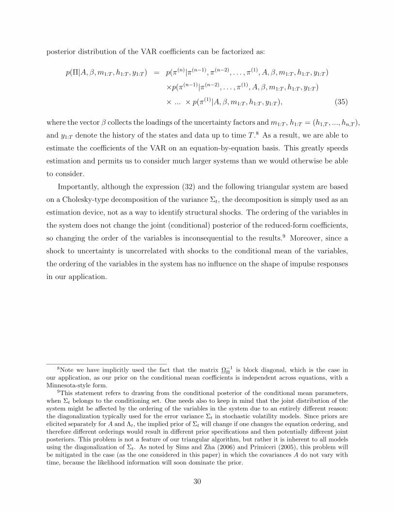
posterior distribution of the VAR coefficients can be factorized as:

p(Π|A, β,m1:T , h1:T , y1:T ) = p(π(n)|π(n−1), π(n−2), . . . , π(1), A, β,m1:T , h1:T , y1:T )

×p(π(n−1)|π(n−2), . . . , π(1), A, β,m1:T , h1:T , y1:T )

× ... × p(π(1)|A, β,m1:T , h1:T , y1:T ), (35)

where the vector β collects the loadings of the uncertainty factors andm1:T , h1:T = (h1,T , ..., hn,T ),

and y1:T denote the history of the states and data up to time T .8 As a result, we are able to

estimate the coefficients of the VAR on an equation-by-equation basis. This greatly speeds

estimation and permits us to consider much larger systems than we would otherwise be able

to consider.

Importantly, although the expression (32) and the following triangular system are based

on a Cholesky-type decomposition of the variance Σt, the decomposition is simply used as an

estimation device, not as a way to identify structural shocks. The ordering of the variables in

the system does not change the joint (conditional) posterior of the reduced-form coefficients,

so changing the order of the variables is inconsequential to the results.9 Moreover, since a

shock to uncertainty is uncorrelated with shocks to the conditional mean of the variables,

the ordering of the variables in the system has no influence on the shape of impulse responses

in our application.

8Note we have implicitly used the fact that the matrix Ω−1Π is block diagonal, which is the case in

our application, as our prior on the conditional mean coefficients is independent across equations, with aMinnesota-style form.

9This statement refers to drawing from the conditional posterior of the conditional mean parameters,when Σt belongs to the conditioning set. One needs also to keep in mind that the joint distribution of thesystem might be affected by the ordering of the variables in the system due to an entirely different reason:the diagonalization typically used for the error variance Σt in stochastic volatility models. Since priors areelicited separately for A and Λt, the implied prior of Σt will change if one changes the equation ordering, andtherefore different orderings would result in different prior specifications and then potentially different jointposteriors. This problem is not a feature of our triangular algorithm, but rather it is inherent to all modelsusing the diagonalization of Σt. As noted by Sims and Zha (2006) and Primiceri (2005), this problem willbe mitigated in the case (as the one considered in this paper) in which the covariances A do not vary withtime, because the likelihood information will soon dominate the prior.

30

8 References

Ahn, Seung C., and Alex R. Horenstein (2013), “Eigenvalue Ratio Test for the Number of

Factors,” Econometrica 81, 1203-1227. DOI:10.3982/ECTA8968

Andrews, Donald W.K., and J. Christopher Monahan (1992), “An Improved Heteroskedas-

ticity and Autocorrelation Consistent Covariance Matrix Estimator,” Econometrica 60,

953-966. DOI:10.2307/2951574

Andrieu, Christophe, Arnaud Doucet, and Roman Holenstein (2010), “Particle Markov

Chain Monte Carlo Methods,” Journal of the Royal Statistical Society, Series B 72,

269-342. DOI:10.1111/j.1467-9868.2009.00736.x

Baker, Scott R., Nicholas Bloom, and Steven J. Davis (2016), “Measuring Economic Pol-

icy Uncertainty,” Quarterly Journal of Economics 131, 1593-1636. DOI:10.1093/qje/

qjw024

Basu, Susanto, and Brent Bundick (2017), “Uncertainty Shocks in a Model of Effective

Demand,” Econometrica 85, 937-958. DOI:10.3982/ECTA13960

Basu, Susanto, John G. Fernald, and Miles S. Kimball (2006), “Are Technology Improve-

ments Contractionary?” American Economic Review 96, 1418-1448. DOI:10.1257/aer.

96.5.1418

Benati, Luca (2016), “Economic Policy Uncertainty, the Great Recession, and the Great

Depression,” manuscript, University of Bern.

Berger, Tino, Sibylle Grabert, and Bernd Kempa (2016), “Global and Country-Specific

Output Growth Uncertainty and Macroeconomic Performance,” Oxford Bulletin of Eco-

nomics and Statistics 78, 694-716. DOI:10.1111/obes.12118

Bloom, Nicholas (2014), “Fluctuations in Uncertainty,” Journal of Economic Perspectives

28, 153-176. DOI:10.1257/jep.28.2.153

Bloom, Nicholas (2009), “The Impact of Uncertainty Shocks,” Econometrica 77, 623-685.

DOI:10.3982/ECTA6248

Caggiano, Giovanni, Efrem Castelnuovo, and Juan Manuel Figueres (2017), “Economic Pol-

icy Uncertainty and Unemployment in the United States: A Nonlinear Approach,” Eco-

nomics Letters 151, 31-34. DOI:10.1016/j.econlet.2016.12.002

Caggiano, Giovanni, Efrem Castelnuovo, and Nicolas Groshenny (2014), “Uncertainty Shocks

and Unemployment Dynamics: An Analysis of Post-WWII US Recessions,” Journal of

Monetary Economics 67, 78-92. DOI:10.1016/j.jmoneco.2014.07.006

31

Caggiano, Giovanni, Efrem Castelnuovo, and Giovanni Pellegrino (2017), “Estimating the

Real Effects of Uncertainty at the Zero Lower Bound,” European Economic Review 100,

257-272. DOI:10.1016/j.euroecorev.2017.08.008

Caldara, Dario, Cristina Fuentes-Albero, Simon Gilchrist, and Egon Zakrajsek (2016), “The

Macroeconomic Impact of Financial and Uncertainty Shocks,” European Economic Re-

view 88, 185-207. DOI:10.1016/j.euroecorev.2016.02.020

Carriere-Swallow, Yan, and Luis Felipe Cespedes (2013), “The Impact of Uncertainty Shocks

in Emerging Economies,” Journal of International Economics 90, 316-325. DOI:10.

1016/j.jinteco.2013.03.003

Carriero, Andrea, Todd E. Clark, and Massimiliano Marcellino (2017), “Measuring Uncer-

tainty and Its Impact on the Economy,” Review of Economics and Statistics, forthcoming.

DOI:10.1162/REST_a_00693

Carriero, Andrea, Todd E. Clark, and Massimiliano Marcellino (2018), “Endogenous Uncer-

tainty,” manuscript.

Carriero, Andrea, Todd E. Clark, and Massimiliano Marcellino (2016a), “Common Drifting

Volatility in Large Bayesian VARs,” Journal of Business and Economic Statistics 34,

375-390. DOI:10.1080/07350015.2015.1040116

Carriero, Andrea, Todd E. Clark, and Massimiliano Marcellino (2016b), “Large Vector Au-

toregressions with Stochastic Volatility and Flexible Priors,” Federal Reserve Bank of

Cleveland Working Paper no. 16-17. DOI:10.26509/frbc-wp-201617

Carriero, Andrea, Todd E. Clark, and Massimiliano Marcellino (2015), “Bayesian VARs:

Specification Choices and Forecasting Performance,” Journal of Applied Econometrics

30, 46-73. DOI:10.1002/jae.2315

Casarin, Roberto, Claudia Foroni, Massimiliano Marcellino, and Francesco Ravazzolo (2017),

“Uncertainty through the Lenses of a Mixed-Frequency Bayesian Panel Markov Switching

Model,” CEPR DP 8339.

Castelnuovo, Efrem, and Trung Duc Tran (2017), “Google it Up! A Google Trends-based

Uncertainty index for the United States and Australia,” Economics Letters 161, 149-153.

DOI:10.1016/j.econlet.2017.09.032

Cesa-Bianchi, Ambrogio, M. Hashem Pesaran, and Alessandro Rebucci (2017), “Uncertainty

and Economic Activity: Identification through Cross-Country Correlations,” manuscript.

Cogley, Timothy, and Thomas J. Sargent (2005), “Drifts and Volatilities: Monetary Policies

32

and Outcomes in the Post-WWII US,” Review of Economic Dynamics 8, 262-302. DOI:

10.1016/j.red.2004.10.009

Coibion, Olivier, Yuriy Gorodnichenko, Lorenz Kueng, and John Silvia (2017), “Innocent

Bystanders? Monetary Policy and Inequality in the U.S.,” Journal of Monetary Eco-

nomics 88, 70-89. DOI:10.1016/j.jmoneco.2017.05.005

Cuaresma, Jesus Crespo, Florian Huber, and Luca Onorante (2017), “The Macroeconomic

Effects of International Uncertainty Shocks,” Working Paper No. 245, Vienna University

of Economics and Business.

Davis, Steven J. (2016), “An Index of Global Economic Policy Uncertainty,” NBER Working

Paper No. 22740. DOI:10.3386/w22740

Del Negro, Marco, and Giorgio E. Primiceri (2015), “Time Varying Structural Vector Au-

toregressions and Monetary Policy: A Corrigendum,” Review of Economic Studies 82,

1342-1345. DOI:10.1093/restud/rdv024

Gilchrist, Simon, Jae W. Sim, and Egon Zakrajsek (2014), “Uncertainty, Financial Frictions,

and Investment Dynamics,” NBER Working Paper no. 20038. DOI:10.3386/w20038

Gourio, Francois, Michael Siemer, and Adrien Verdelhan (2013), “International Risk Cycles,”

Journal of International Economics 89, 471-484. DOI:10.1016/j.jinteco.2011.10.

001

Gurkaynak, Refet S., Brian Sack, and Eric T. Swanson (2005), “Do Actions Speak Louder

Than Words? The Response of Asset Prices to Monetary Policy Actions and State-

ments,” International Journal of Central Banking 1, 55-93.

Hamilton, James D. (2003), “What Is an Oil Shock?” Journal of Econometrics 113, 363-398.

DOI:10.1016/S0304-4076(02)00207-5

Jarocinski, Marek, and Bartosz Mackowiak (2017), “Granger Causal Priority and Choice of

Variables in Vector Autoregressions,” Review of Economics and Statistics 99, 319-329.

DOI:10.1162/REST_a_00601

Jo, Soojin, and Rodrigo Sekkel (2017), “Macroeconomic Uncertainty through the Lens of

Professional Forecasters,” Journal of Business and Economic Statistics, forthcoming.

DOI:10.1080/07350015.2017.1356729

Jurado, Kyle, Sydney C. Ludvigson, and Serena Ng (2015), “Measuring Uncertainty,” Amer-

ican Economic Review 105, 1177-1216. DOI:10.1257/aer.20131193

Kilian, Lutz (2008), “Exogenous Oil Supply Shocks: How Big Are They and How Much Do

33

They Matter for the U.S. Economy?” Review of Economics and Statistics 90, 216-240.

DOI:10.1162/rest.90.2.216

Kim, Sangjoon, Neil Shephard, and Siddhartha Chib (1998), “Stochastic Volatility: Likeli-

hood Inference and Comparison with ARCH Models,” Review of Economic Studies 65,

361-393. DOI:10.1111/1467-937X.00050

Leduc, Sylvain, and Zheng Liu (2016), “Uncertainty Shocks Are Aggregate Demand Shocks,”

Journal of Monetary Economics 82, 20-35. DOI:10.1016/j.jmoneco.2016.07.002

Ludvigson, Sydney C., Sai Ma, and Serena Ng (2016), “Uncertainty and Business Cycles:

Exogenous Impulse or Endogenous Response?” manuscript, New York University.

Mertens, Karel, and Morten O. Ravn (2012), “Empirical Evidence on the Aggregate Effects

of Anticipated and Unanticipated U.S. Tax Policy Shocks,” American Economic Journal:

Economic Policy 4, 145-181. DOI:10.1257/pol.4.2.145

Mumtaz, Haroon, and Konstantinos Theodoridis (2017), “Common and Country Specific

Economic Uncertainty,” Journal of International Economics 105, 205-216. DOI:10.

1016/j.jinteco.2017.01.007

OECD (2017), Quarterly GDP (indicator). DOI:10.1787/b86d1fc8-en (Accessed on 28

March 2017)

Omori, Yasuhiro, Siddhartha Chib, Neil Shephard, and Juichi Nakajima (2007), “Stochastic

Volatility with Leverage: Fast and Efficient Likelihood Inference,” Journal of Economet-

rics 140, 425-449. DOI:10.1016/j.jeconom.2006.07.008

Otrok, Christopher, and Charles H. Whiteman (1998), “Bayesian Leading Indicators: Mea-

suring and Predicting Economic Conditions in Iowa,” International Economic Review

39, 997-1014. DOI:10.2307/2527349

Primiceri, Giorgio E. (2005), “Time-Varying Structural Vector Autoregressions and Mon-

etary Policy,” Review of Economic Studies 72, 821-852. DOI:10.1111/j.1467-937X.

2005.00353.x

Ramey, Valerie A. (2011), “Identifying Government Spending Shocks: It’s All in the Timing,”

Quarterly Journal of Economics 126, 1-50. DOI:10.1093/qje/qjq008

Romer, Christina D., and David H. Romer (2004), “A New Measure of Monetary Shocks:

Derivation and Implications,” American Economic Review 94, 1055-1084. DOI:10.1257/

0002828042002651

Shin, Minchul, and Molin Zhong (2016), “A New Approach to Identifying the Real Effects

34

of Uncertainty Shocks,” manuscript.

Sims, Christopher A., and Tao Zha (2006), “Were There Regime Switches in U.S. Monetary

Policy?” American Economic Review 96, 54-81. DOI:10.1257/000282806776157678

Stock, James H., and Mark W. Watson (2016), “Factor Models for Macroeconomics” (pp.

415-525), in John B. Taylor and Harald Uhlig, eds., Handbook of Macroeconomics, Vol.

2 (Amsterdam: North Holland). DOI:10.1016/bs.hesmac.2016.04.002

Stock, James H., and Mark W. Watson (2012), “Disentangling the Channels of the 2007-

2009 Recession,” Brookings Papers on Economic Activity (2012), Spring, 81-130. DOI:

10.1353/eca.2012.0005

35

Table 1: Variables in the 3-economy macroeconomic dataset

U.S. variables E.A. variables U.K. variablesreal GDP (∆ ln) real GDP (∆ ln) real GDP (∆ ln)real consumption (∆ ln) real consumption (∆ ln) real consumption (∆ ln)real government consumption (∆ ln) real government consumption (∆ ln) real government consumption (∆ ln)real investment (∆ ln) real investment (∆ ln) real investment (∆ ln)real exports (∆ ln) real exports (∆ ln) real exports (∆ ln)real imports (∆ ln) real imports (∆ ln) real imports (∆ ln)real inventories real inventories unit labor costs (∆ ln)unit labor costs (∆ ln) unit labor costs (∆ ln) industrial confidenceemployment (∆ ln) employment (∆ ln) consumer confidencehours worked (∆ ln) unemployment rate employment (∆ ln)unemployment rate Eonia rate unemployment rateFederal funds rate 2-year bond yield producer prices (∆ ln)2-year bond yield 10-year bond yield retail price index (∆ ln)10-year bond yield M3 (∆ ln) official bank rateM2 (∆ ln) GDP deflator (∆ ln) 10-year bond yieldoil price (∆ ln) consumer prices (∆ ln) stock price index (∆ ln)commodity prices (∆ ln) core consumer prices (∆ ln)consumer prices (∆ ln) producer prices (∆ ln)core consumer prices (∆ ln) real housing investment (∆ ln)producer prices (∆ ln) stock price index (∆ ln)real housing investment (∆ ln) capacity utilizationstock price index (∆ ln) consumer confidencecapacity utilization industrial confidenceconsumer confidence purchasing managers’ indexindustrial confidence labor shortagespurchasing managers’ index

Note: For those variables transformed for use in the model, the table indicates the trans-formation in parentheses following the variable description.

36

Table 2: Summary statistics on commonality in volatility

19-country GDP dataset 3-economy macroeconomic datasetPrin. comp. R2 A-H ratio R2 A-H ratio

1 0.786 7.431 0.417 1.6212 0.106 1.746 0.258 2.4523 0.061 3.041 0.105 1.7894 0.020 1.905 0.059 1.1935 0.010 1.296 0.049 1.275

37

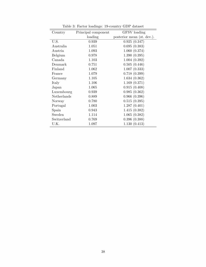
Table 3: Factor loadings: 19-country GDP dataset

Country Principal component GFSV loadingloading posterior mean (st. dev.).

U.S. 0.939 0.925 (0.347)Australia 1.051 0.695 (0.383)Austria 1.093 1.060 (0.374)Belgium 0.978 1.390 (0.395)Canada 1.103 1.004 (0.392)Denmark 0.751 0.505 (0.446)Finland 1.062 1.007 (0.333)France 1.079 0.718 (0.399)Germany 1.105 1.634 (0.362)Italy 1.106 1.169 (0.371)Japan 1.065 0.915 (0.408)Luxembourg 0.939 0.985 (0.362)Netherlands 0.889 0.966 (0.396)Norway 0.780 0.515 (0.395)Portugal 1.003 1.287 (0.401)Spain 0.943 1.415 (0.382)Sweden 1.114 1.065 (0.382)Switzerland 0.769 0.396 (0.388)U.K. 1.097 1.130 (0.413)

38

Tab

le4:

Load

ings

on

firs

tfa

ctor:

3-e

con

om

ym

acr

oec

on

om

icd

ata

set

Cou

ntr

yP

rin

cip

al

com

pon

ent

GF

SV

load

ing

Cou

ntr

yP

rin

cip

al

com

pon

ent

GF

SV

load

ing

load

ing

post

erio

rm

ean

(st.

dev

.)lo

ad

ing

post

erio

rm

ean

(st.

dev

.)U

.S.

real

GD

P1.3

30

0.4

55

(0.2

74)

E.A

.em

plo

ym

ent

0.7

99

0.8

45

(0.4

11)

U.S

.re

al

con

sum

pti

on

1.2

39

0.6

40

(0.3

18)

E.A

.u

nem

plo

ym

ent

rate

0.6

52

1.0

02

(0.3

71)

U.S

.re

al

gover

nm

ent

con

sum

pti

on

1.2

81

0.5

63

(0.3

16)

E.A

.E

on

iara

te0.8

46

1.4

60

(0.3

69)

U.S

.re

al

inves

tmen

t1.2

46

0.2

11

(0.3

42)

E.A

.2-y

ear

bon

dyie

ld1.3

21

0.6

65

(0.3

64)

U.S

.re

al

exp

ort

s1.2

65

0.5

16

(0.3

27)

E.A

.10-y

ear

bon

dyie

ld0.2

90

0.5

58

(0.3

84)

U.S

.re

al

imp

ort

s1.2

91

0.6

78

(0.3

34)

E.A

.M

31.1

64

0.8

66

(0.3

55)

U.S

.re

al

inven

tori

es1.3

28

0.3

26

(0.3

61)

E.A

.G

DP

defl

ato

r0.9

55

0.9

66

(0.4

00)

U.S

.u

nit

lab

or

cost

s0.9

15

0.5

79

(0.3

16)

E.A

.co

nsu

mer

pri

ces

1.3

31

0.8

24

(0.3

80)

U.S

.em

plo

ym

ent

1.0

32

0.1

25

(0.3

76)

E.A

.co

reco

nsu

mer

pri

ces

-0.5

59

0.4

49

(0.3

94)

U.S

.h

ou

rsw

ork

ed-1

.168

0.2

99

(0.3

23)

E.A

.p

rod

uce

rp

rice

s1.2

13

0.6

96

(0.4

26)

U.S

.u

nem

plo

ym

ent

rate

1.3

24

0.7

72

(0.3

72)

E.A

.re

al

hou

sin

gin

ves

tmen

t1.1

80

1.3

41

(0.3

85)

U.S

.F

eder

al

fun

ds

rate

1.3

53

1.2

39

(0.3

33)

E.A

.st

ock

pri

cein

dex

0.6

13

0.5

79

(0.3

99)

U.S

.2-y

ear

bon

dyie

ld0.9

02

0.3

35

(0.3

37)

E.A

.ca

paci

tyu

tiliza

tion

0.3

90

0.6

29

(0.3

89)

U.S

.10-y

ear

bon

dyie

ld0.4

62

0.4

14

(0.3

49)

E.A

.co

nsu

mer

con

fid

ence

0.8

36

0.5

74

(0.4

05)

U.S

.M

20.8

22

0.6

04

(0.3

63)

E.A

.in

dust

rial

con

fid

ence

1.0

07

0.3

86

(0.4

07)

oil

pri

ce1.3

44

1.2

45

(0.3

17)

E.A

.p

urc

hasi

ng

man

ager

s’in

dex

-0.9

52

0.4

49

(0.4

02)

com

mod

ity

pri

ces

1.3

47

1.0

30

(0.2

87)

E.A

.la

bor

short

ages

0.7

19

1.3

68

(0.3

92)

U.S

.co

nsu

mer

pri

ces

1.1

94

1.0

06

(0.3

51)

U.K

.re

al

GD

P1.1

88

0.7

36

(0.4

06)

U.S

.co

reco

nsu

mer

pri

ces

1.1

86

0.7

97

(0.3

13)

U.K

.re

al

con

sum

pti

on

0.6

15

0.8

81

(0.3

91)

U.S

.p

rod

uce

rp

rice

s1.0

69

0.6

05

(0.3

67)

U.K

.re

al

gover

nm

ent

con

sum

pti

on

0.0

59

0.3

86

(0.3

97)

U.S

.re

al

hou

sin

gin

ves

tmen

t0.8

80

0.8

96

(0.4

03)

U.K

.re

al

inves

tmen

t1.1

05

0.5

26

(0.3

79)

U.S

.st

ock

pri

cein

dex

1.2

08

1.1

74

(0.3

95)

U.K

.re

al

exp

ort

s0.0

07

0.6

44

(0.3

87)

U.S

.ca

paci

tyu

tiliza

tion

1.3

60

0.7

28

(0.3

74)

U.K

.re

al

imp

ort

s0.6

41

0.7

29

(0.4

06)

U.S

.co

nsu

mer

con

fid

ence

1.3

19

0.8

99

(0.3

63)

U.K

.u

nit

lab

or

cost

s0.0

18

0.5

22

(0.4

04)

U.S

.in

du

stri

al

con

fid

ence

1.2

69

0.5

59

(0.3

75)

U.K

.in

du

stri

al

con

fid

ence

-1.1

29

0.5

88

(0.4

01)

U.S

.p

urc

hasi

ng

man

ager

s’in

dex

1.3

63

0.8

96

(0.3

51)

U.K

.co

nsu

mer

con

fid

ence

0.8

75

0.8

46

(0.3

92)

E.A

.re

al

GD

P1.2

88

1.4

97

(0.3

35)

U.K

.em

plo

ym

ent

0.1

64

0.7

75

(0.3

91)

E.A

.re

al

con

sum

pti

on

0.7

01

0.9

61

(0.3

70)

U.K

.u

nem

plo

ym

ent

rate

0.1

65

0.7

21

(0.4

10)

E.A

.re

al

gover

nm

ent

con

sum

pti

on

0.4

37

0.6

85

(0.4

16)

U.K

.p

rod

uce

rp

rice

s1.0

96

0.8

16

(0.4

14)

E.A

.re

al

inves

tmen

t0.8

17

0.2

59

(0.3

76)

U.K

.re

tail

pri

cein

dex

0.9

45

1.0

48

(0.4

25)

E.A

.re

al

exp

ort

s1.0

38

1.0

45

(0.3

87)

U.K

.offi

cial

ban

kra

te0.8

76

0.9

87

(0.4

12)

E.A

.re

al

imp

ort

s1.0

90

0.6

86

(0.3

86)

U.K

.10-y

ear

bon

dyie

ld0.2

52

0.9

06

(0.4

04)

E.A

.re

al

inven

tori

es1.0

59

0.8

40

(0.3

63)

U.K

.st

ock

pri

cein

dex

0.4

83

0.8

75

(0.4

14)

E.A

.u

nit

lab

or

cost

s0.6

89

0.8

49

(0.3

66)

39

Table 5: Correlations of uncertainty shocks with other shocks

19-country 3-economyknown GDP dataset macro datasetshock uncert. shock uncert. shock

Productivity: Fernald TFP -0.097 -0.049(1985:Q1-2016:Q3, 1985:Q4-2013:Q3) (0.279) (0.496)Oil supply: Hamilton (2003) 0.056 -0.017(1985:Q1-2016:Q3, 1985:Q4-2013:Q3) (0.561) (0.812)Oil supply: Kilian (2008) -0.038 0.022(1985:Q1-2004:Q3, 1985:Q4-2004:Q3) (0.776) (0.834)Monetary policy: Guykaynak, et al. (2005) -0.070 -0.112(1990:Q1-2004:Q4, 1990:Q1-2004:Q4) (0.359) (0.284)Monetary policy: Coibion, et al. (2016) -0.181 -0.046(1985:Q1-2008:Q4, 1985:Q4-2008:Q4) (0.036) (0.589)Fiscal policy: Ramey (2011) -0.175 0.050(1985:Q1-2008:Q4, 1985:Q4-2008:Q4) (0.239) (0.649)Fiscal policy: Mertens and Ravn (2012) 0.198 0.013(1985:Q1-2006:Q4, 1985:Q4-2006:Q4) (0.002) (0.845)

Notes: The table provides the correlations of the shocks to uncertainty (measured as theposterior medians of um,t) with selected macroeconomic shocks for the U.S. Entries inparentheses provide (in column 1) the sample periods of the correlation estimates, first forthe 19-country GDP dataset and then for the 3-economy macroeconomic dataset and (incolumns 2 and 3) the p-values of t-statistics of the coefficient obtained by regressing theuncertainty shock on the macroeconomic shock (and a constant). The variances underlyingthe t-statistics are computed with the prewhitened quadratic spectral estimator of Andrewsand Monahan (1992).

40

U.S.

E.A.

U.K.

real

GD

P

1985

1988

1991

1994

1997

2000

2003

2006

2009

2012

0.25

0.50

0.75

1.00

1.25

1.50

1.75

real

con

sum

ptio

n

1985

1988

1991

1994

1997

2000

2003

2006

2009

2012

0.4

0.6

0.8

1.0

1.2

1.4

real

inve

stm

ent

1985

1988

1991

1994

1997

2000

2003

2006

2009

2012

0.4

0.6

0.8

1.0

1.2

1.4

1.6

real

exp

orts

1985

1988

1991

1994

1997

2000

2003

2006

2009

2012

0.4

0.6

0.8

1.0

1.2

1.4

1.6

1.8

unit

labo

r cos

ts

1985

1988

1991

1994

1997

2000

2003

2006

2009

2012

0.4

0.6

0.8

1.0

1.2

1.4

1.6

empl

oym

ent

1985

1988

1991

1994

1997

2000

2003

2006

2009

2012

0.2

0.4

0.6

0.8

1.0

1.2

unem

ploy

men

t rat

e

1985

1988

1991

1994

1997

2000

2003

2006

2009

2012

0.06

0.08

0.10

0.12

0.14

0.16

0.18

0.20

0.22

cons

umer

pric

es

1985

1988

1991

1994

1997

2000

2003

2006

2009

2012

0.50

0.75

1.00

1.25

1.50

1.75

2.00

2.25

prod

ucer

pric

es

1985

1988

1991

1994

1997

2000

2003

2006

2009

2012

0.50

0.75

1.00

1.25

1.50

1.75

2.00

2.25

polic

y ra

te

1985

1988

1991

1994

1997

2000

2003

2006

2009

2012

0.00

0.05

0.10

0.15

0.20

0.25

0.30

0.35

0.40

10-y

ear b

ond

yiel

d

1985

1988

1991

1994

1997

2000

2003

2006

2009

2012

0.10

0

0.12

5

0.15

0

0.17

5

0.20

0

0.22

5

0.25

0

0.27

5

0.30

0

stoc

k pr

ice

inde

x

1985

1988

1991

1994

1997

2000

2003

2006

2009

2012

0.75

1.00

1.25

1.50

1.75

2.00

Figure 1: BVAR-SV estimates of volatilities (standard deviations), selected variables

41

uncertainty factor m(t)^0.5 PC of BVAR-SV 15%ile 85%ile

1985 1987 1989 1991 1993 1995 1997 1999 2001 2003 2005 2007 2009 2011 2013 20150.0

0.5

1.0

1.5

2.0

2.5

3.0

3.5

Black MondayGulf War I

Asian Crisis

Russian Crisis9/11

Enron

Gulf War IICrisis

correlation = 0.641

uncertainty factor m(t)^0.5 PC of BVAR-SV 15%ile 85%ile

1985 1987 1989 1991 1993 1995 1997 1999 2001 2003 2005 2007 2009 2011 20130.0

0.5

1.0

1.5

2.0

2.5

3.0

3.5

4.0

4.5

Black MondayGulf War I

Asian Crisis

Russian Crisis9/11

Enron

Gulf War IICrisis

correlation = 0.800

Figure 2: Uncertainty estimates for 19-country GDP dataset in the top panel and for 3-economymacroeconomic dataset in the bottom panel. In each panel, the blue line provides an estimateobtained from the first principal component of the BVAR-SV estimates of log volatility. Thesolid black line and gray-shaded regions provide the posterior median and 15%/85% quantiles ofthe BVAR-GFSV estimate of macroeconomic uncertainty (m0.5

t ). The periods indicated by blackvertical lines or regions correspond to the uncertainty events highlighted in Bloom (2009). Labelsfor these events are indicated in text horizontally centered on the event’s start date.

42

19-c

ount

ry G

DP

3-ec

onom

y (le

ft)19

-cou

ntry

GD

P (ri

ght)

1985

1987

1989

1991

1993

1995

1997

1999

2001

2003

2005

2007

2009

2011

2013

0.50

0.75

1.00

1.25

1.50

1.75

2.00

2.25

2.50

2.75

0.75

1.00

1.25

1.50

1.75

2.00

2.25

corr

elat

ion

= 0

.794

CC

M m

acro

3-ec

onom

y (le

ft)C

CM

mac

ro (r

ight

)

1985

1987

1989

1991

1993

1995

1997

1999

2001

2003

2005

2007

2009

2011

2013

0.50

0.75

1.00

1.25

1.50

1.75

2.00

2.25

2.50

2.75

0.8

0.9

1.0

1.1

1.2

1.3

1.4

1.5

1.6

corr

elat

ion

= 0

.695

CC

M fi

nanc

ial

3-ec

onom

y (le

ft)C

CM

fina

ncia

l (rig

ht)

1985

1987

1989

1991

1993

1995

1997

1999

2001

2003

2005

2007

2009

2011

2013

0.50

0.75

1.00

1.25

1.50

1.75

2.00

2.25

2.50

2.75

0.5

1.0

1.5

2.0

2.5

3.0

3.5

corr

elat

ion

= 0

.179

JLN

mac

ro

3-ec

onom

y (le

ft)JL

N m

acro

(rig

ht)

1985

1987

1989

1991

1993

1995

1997

1999

2001

2003

2005

2007

2009

2011

2013

0.50

0.75

1.00

1.25

1.50

1.75

2.00

2.25

2.50

2.75

0.5

0.6

0.7

0.8

0.9

1.0

1.1

corr

elat

ion

= 0

.467

JLN

fina

ncia

l

3-ec

onom

y (le

ft)JL

N fi

nanc

ial (

right

)

1985

1987

1989

1991

1993

1995

1997

1999

2001

2003

2005

2007

2009

2011

2013

0.50

0.75

1.00

1.25

1.50

1.75

2.00

2.25

2.50

2.75

0.6

0.7

0.8

0.9

1.0

1.1

1.2

1.3

1.4

1.5

corr

elat

ion

= 0

.313

glob

al E

PU

3-ec

onom

y (le

ft)gl

obal

EPU

(rig

ht)

1997

1998

1999

2000

2001

2002

2003

2004

2005

2006

2007

2008

2009

2010

2011

2012

2013

0.50

0.75

1.00

1.25

1.50

1.75

2.00

2.25

2.50

2.75

5075100

125

150

175

200

corr

elat

ion

= 0

.365

MT

com

mon

3-ec

onom

y (le

ft)M

T co

mm

on (r

ight

)

1985

1987

1989

1991

1993

1995

1997

1999

2001

2003

2005

2007

2009

2011

2013

0.50

0.75

1.00

1.25

1.50

1.75

2.00

2.25

2.50

2.75

012345678co

rrel

atio

n =

0.5

22

BG

K c

omm

on

3-ec

onom

y (le

ft)BG

K co

mm

on (r

ight

)

1985

1987

1989

1991

1993

1995

1997

1999

2001

2003

2005

2007

2009

2011

2013

0.50

0.75

1.00

1.25

1.50

1.75

2.00

2.25

2.50

2.75

0.5

1.0

1.5

2.0

2.5

3.0

3.5

corr

elat

ion

= 0

.321

Figure 3: Comparison of uncertainty estimates to others in the literature. The top left panelcompares the uncertainty estimate obtained from the 3-economy macroeconomic dataset (blackline) to that obtained with the 19-country GDP dataset (blue line). Other panels compare the3-economy macroeconomic dataset estimate (black line) to a different estimate (blue line) from theliterature, including: CCM macro and financial uncertainty from Carriero, Clark, and Marcellino(2017a); JLN macro and financial uncertainty, 1-step ahead, from Jurado, Ludvigson, and Ng(2015); global economic policy uncertainty (EPU) from Davis (2016); common uncertainty fromMumtaz and Theodoridis (2017); and common uncertainty from Berger, Grabert, and Kempa(2016).

43

U.S

.

05

1015

-0.7

-0.6

-0.5

-0.4

-0.3

-0.2

-0.1

Aus

tral

ia

05

1015

-0.40

-0.35

-0.30

-0.25

-0.20

-0.15

-0.10

-0.05

-0.00

0.05

Aus

tria

05

1015

-0.6

-0.5

-0.4

-0.3

-0.2

-0.1

-0.0

Bel

gium

05

1015

-0.45

-0.40

-0.35

-0.30

-0.25

-0.20

-0.15

-0.10

-0.05

-0.00

Can

ada

05

1015

-0.7

-0.6

-0.5

-0.4

-0.3

-0.2

-0.1

-0.0

Den

mar

k

05

1015

-0.7

-0.6

-0.5

-0.4

-0.3

-0.2

-0.1

-0.00.1

Finl

and

05

1015

-1.2

-1.0

-0.8

-0.6

-0.4

-0.2

-0.0

Fran

ce

05

1015

-0.6

-0.5

-0.4

-0.3

-0.2

-0.1

-0.0

Ger

man

y

05

1015

-0.6

-0.5

-0.4

-0.3

-0.2

-0.1

-0.0

Italy

05

1015

-0.6

-0.5

-0.4

-0.3

-0.2

-0.1

-0.00.1

Japa

n

05

1015

-0.5

-0.4

-0.3

-0.2

-0.1

-0.00.1

0.2

Luxe

mbo

urg

05

1015

-0.6

-0.5

-0.4

-0.3

-0.2

-0.1

-0.00.1

0.2

Net

herla

nds

05

1015

-0.7

-0.6

-0.5

-0.4

-0.3

-0.2

-0.1

-0.0

Nor

way

05

1015

-0.3

-0.2

-0.10.0

0.1

0.2

0.3

Port

ugal

05

1015

-0.6

-0.5

-0.4

-0.3

-0.2

-0.1

-0.00.1

Spai

n

05

1015

-0.9

-0.8

-0.7

-0.6

-0.5

-0.4

-0.3

-0.2

-0.1

-0.0

Swed

en

05

1015

-0.9

-0.8

-0.7

-0.6

-0.5

-0.4

-0.3

-0.2

-0.1

Switz

erla

nd

05

1015

-0.5

-0.4

-0.3

-0.2

-0.1

-0.0

U.K

.

05

1015

-0.6

-0.5

-0.4

-0.3

-0.2

-0.1

-0.0

inte

rnat

iona

l unc

erta

inty

fact

or

05

1015

-0.025

0.00

0

0.02

5

0.05

0

0.07

5

0.10

0

0.12

5

0.15

0

0.17

5

Figure 4: Impulse responses for international uncertainty shock: BVAR-GFSV estimates for 19-country GDP dataset

44

U.S

. rea

l GD

P

05

1015

-0.45

-0.40

-0.35

-0.30

-0.25

-0.20

-0.15

-0.10

-0.05

-0.00

U.S

. rea

l con

sum

ptio

n

05

1015

-0.35

-0.30

-0.25

-0.20

-0.15

-0.10

-0.05

-0.00

U.S

. rea

l gov

ernm

ent c

onsu

mpt

ion

05

1015

-0.4

-0.3

-0.2

-0.1

-0.00.1

0.2

U.S

. rea

l inv

estm

ent

05

1015

-1.4

-1.2

-1.0

-0.8

-0.6

-0.4

-0.2

-0.00.2

U.S

. rea

l exp

orts

05

1015

-1.2

-1.0

-0.8

-0.6

-0.4

-0.2

-0.00.2

U.S

. rea

l im

port

s

05

1015

-1.25

-1.00

-0.75

-0.50

-0.25

0.00

U.S

. rea

l inv

ento

ries

05

1015

-0.100

-0.075

-0.050

-0.025

-0.000

0.02

5

U.S

. uni

t lab

or c

osts

05

1015

-0.4

-0.3

-0.2

-0.1

-0.00.1

0.2

U.S

. em

ploy

men

t

05

1015

-0.40

-0.35

-0.30

-0.25

-0.20

-0.15

-0.10

-0.05

-0.00

U.S

. hou

rs w

orke

d

05

1015

-0.125

-0.100

-0.075

-0.050

-0.025

-0.000

0.02

5

U.S

. une

mpl

oym

ent r

ate

05

1015

-0.025

0.00

00.02

50.05

00.07

50.10

00.12

50.15

00.17

5

U.S

. fed

eral

fund

s ra

te

05

1015

-0.150

-0.125

-0.100

-0.075

-0.050

-0.025

-0.000

0.02

5

U.S

. 2-y

ear b

ond

yiel

d

05

1015

-0.125

-0.100

-0.075

-0.050

-0.025

-0.000

0.02

5

U.S

. 10-

year

bon

d yi

eld

05

1015

-0.075

-0.050

-0.025

0.00

0

0.02

5

0.05

0

U.S

. M2

05

1015

-0.25

-0.20

-0.15

-0.10

-0.05

-0.00

0.05

0.10

0.15

0.20

oil p

rice

05

1015

-7-6-5-4-3-2-101

com

mod

ity p

rices

05

1015

-1.5

-1.0

-0.50.0

0.5

1.0

1.5

U.S

. con

sum

er p

rices

05

1015

-0.25

-0.20

-0.15

-0.10

-0.05

-0.00

0.05

U.S

. cor

e co

nsum

er p

rices

05

1015

-0.06

-0.04

-0.02

0.00

0.02

0.04

0.06

0.08

0.10

U.S

. pro

duce

r pric

es

05

1015

-0.4

-0.3

-0.2

-0.1

-0.00.1

0.2

Figure 5: Impulse responses for international uncertainty shock: BVAR-GFSV estimates for 3-economy macroeconomic dataset

45

U.S

. rea

l hou

sing

inve

stm

ent

05

1015

-1.5

-1.0

-0.50.0

0.5

1.0

1.5

U.S

. sto

ck p

rice

inde

x

05

1015

-2.0

-1.5

-1.0

-0.50.0

0.5

1.0

1.5

U.S

. cap

acity

util

izat

ion

05

1015

-1.50

-1.25

-1.00

-0.75

-0.50

-0.25

0.00

0.25

0.50

U.S

. con

sum

er c

onfid

ence

05

1015

-3.0

-2.5

-2.0

-1.5

-1.0

-0.50.0

0.5

U.S

. ind

ustr

ial c

onfid

ence

05

1015

-2.5

-2.0

-1.5

-1.0

-0.50.0

0.5

1.0

U.S

. pur

chas

ing

man

ager

s' in

dex

05

1015

-1.50

-1.25

-1.00

-0.75

-0.50

-0.25

0.00

0.25

0.50

E.A

. rea

l GD

P

05

1015

-0.40

-0.35

-0.30

-0.25

-0.20

-0.15

-0.10

-0.05

-0.00

E.A

. rea

l con

sum

ptio

n

05

1015

-0.20

-0.15

-0.10

-0.05

-0.00

0.05

0.10

E.A

. rea

l gov

ernm

ent c

onsu

mpt

ion

05

1015

-0.20

-0.15

-0.10

-0.05

-0.00

0.05

0.10

E.A

. rea

l inv

estm

ent

05

1015

-0.9

-0.8

-0.7

-0.6

-0.5

-0.4

-0.3

-0.2

-0.1

-0.0

E.A

. rea

l exp

orts

05

1015

-1.2

-1.0

-0.8

-0.6

-0.4

-0.2

-0.0

E.A

. rea

l im

port

s

05

1015

-0.9

-0.8

-0.7

-0.6

-0.5

-0.4

-0.3

-0.2

-0.1

-0.0

E.A

. rea

l inv

ento

ries

05

1015

-0.04

-0.03

-0.02

-0.01

0.00

0.01

0.02

0.03

E.A

. uni

t lab

or c

osts

05

1015

-0.05

0.00

0.05

0.10

0.15

0.20

0.25

0.30

E.A

. em

ploy

men

t

05

1015

-0.30

-0.25

-0.20

-0.15

-0.10

-0.05

-0.00

0.05

E.A

. une

mpl

oym

ent r

ate

05

1015

-0.02

0.00

0.02

0.04

0.06

0.08

0.10

0.12

E.A

. Eon

ia ra

te

05

1015

-0.100

-0.075

-0.050

-0.025

-0.000

0.02

5

0.05

0

0.07

5

E.A

. 2-y

ear b

ond

yiel

d

05

1015

-0.100

-0.075

-0.050

-0.025

-0.000

0.02

5

0.05

0

0.07

5

E.A

. 10-

year

bon

d yi

eld

05

1015

-0.04

-0.02

0.00

0.02

0.04

0.06

0.08

0.10

E.A

. M3

05

1015

-0.7

-0.6

-0.5

-0.4

-0.3

-0.2

-0.1

-0.00.1

Figure 5: Continued, impulse responses for international uncertainty shock: BVAR-GFSV estimatesfor 3-economy macroeconomic dataset

46

E.A

. GD

P de

flato

r

05

1015

-0.050

-0.025

0.00

00.02

50.05

00.07

50.10

00.12

50.15

00.17

5

E.A

. con

sum

er p

rices

05

1015

-0.150

-0.125

-0.100

-0.075

-0.050

-0.025

-0.000

0.02

50.05

00.07

5

E.A

. cor

e co

nsum

er p

rices

05

1015

-0.02

0.00

0.02

0.04

0.06

0.08

0.10

0.12

0.14

0.16

E.A

. pro

duce

r pric

es

05

1015

-0.6

-0.5

-0.4

-0.3

-0.2

-0.1

-0.00.1

E.A

. rea

l hou

sing

inve

stm

ent

05

1015

-1.2

-1.0

-0.8

-0.6

-0.4

-0.2

-0.0

E.A

. sto

ck p

rice

inde

x

05

1015

-5-4-3-2-101

E.A

. cap

acity

util

izat

ion

05

1015

-0.35

-0.30

-0.25

-0.20

-0.15

-0.10

-0.05

-0.00

0.05

E.A

. con

sum

er c

onfid

ence

05

1015

-0.7

-0.6

-0.5

-0.4

-0.3

-0.2

-0.1

-0.00.1

E.A

. ind

ustr

ial c

onfid

ence

05

1015

-1.00

-0.75

-0.50

-0.25

0.00

0.25

E.A

. pur

chas

ing

man

ager

s' in

dex

05

1015

-0.6

-0.5

-0.4

-0.3

-0.2

-0.1

-0.00.1

0.2

E.A

. lab

or s

hort

ages

05

1015

-0.20

-0.15

-0.10

-0.05

-0.00

0.05

0.10

0.15

U.K

. rea

l GD

P

05

1015

-0.35

-0.30

-0.25

-0.20

-0.15

-0.10

-0.05

-0.00

0.05

0.10

U.K

. rea

l con

sum

ptio

n

05

1015

-0.6

-0.5

-0.4

-0.3

-0.2

-0.1

-0.00.1

U.K

. rea

l gov

ernm

ent c

onsu

mpt

ion

05

1015

-0.5

-0.4

-0.3

-0.2

-0.1

-0.00.1

U.K

. rea

l inv

estm

ent

05

1015

-1.25

-1.00

-0.75

-0.50

-0.25

0.00

0.25

0.50

U.K

. rea

l exp

orts

05

1015

-1.50

-1.25

-1.00

-0.75

-0.50

-0.25

0.00

0.25

U.K

. rea

l im

port

s

05

1015

-1.25

-1.00

-0.75

-0.50

-0.25

0.00

0.25

U.K

. uni

t lab

or c

osts

05

1015

-0.4

-0.3

-0.2

-0.1

-0.00.1

0.2

0.3

U.K

. ind

ustr

ial c

onfid

ence

05

1015

-4-3-2-1012

U.K

. con

sum

er c

onfid

ence

05

1015

-1.50

-1.25

-1.00

-0.75

-0.50

-0.25

0.00

0.25

Figure 5: Continued, impulse responses for international uncertainty shock: BVAR-GFSV estimatesfor 3-economy macroeconomic dataset

47

U.K

. em

ploy

men

t

05

1015

-0.20

-0.15

-0.10

-0.05

-0.00

0.05

U.K

. une

mpl

oym

ent r

ate

05

1015

-0.02

0.00

0.02

0.04

0.06

0.08

0.10

0.12

0.14

U.K

. pro

duce

r pric

es

05

1015

-0.15

-0.10

-0.05

0.00

0.05

0.10

0.15

0.20

0.25

0.30

U.K

. ret

ail p

rice

inde

x

05

1015

-0.2

-0.10.0

0.1

0.2

0.3

0.4

U.K

. offi

cial

ban

k ra

te

05

1015

-0.125

-0.100

-0.075

-0.050

-0.025

-0.000

0.02

50.05

00.07

50.10

0

U.K

. 10-

year

bon

d yi

eld

05

1015

-0.06

-0.04

-0.02

0.00

0.02

0.04

0.06

0.08

0.10

U.K

. sto

ck p

rice

inde

x

05

1015

-2.0

-1.5

-1.0

-0.50.0

0.5

1.0

1.5

inte

rnat

iona

l unc

erta

inty

fact

or 1

05

1015

-0.025

0.00

00.02

50.05

00.07

50.10

00.12

50.15

00.17

5

inte

rnat

iona

l unc

erta

inty

fact

or 2

05

1015

-0.100

-0.075

-0.050

-0.025

-0.000

0.02

50.05

00.07

50.10

00.12

5

Figure 5: Continued, impulse responses for international uncertainty shock: BVAR-GFSV estimatesfor 3-economy macroeconomic dataset

48

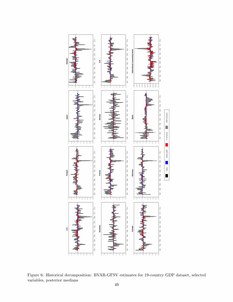
data

base

pat

hm

sho

cks

VAR

shoc

ks

U.S

.

1987

1990

1993

1996

1999

2002

2005

2008

2011

2014

-5-4-3-2-10123

Aus

tral

ia

1987

1990

1993

1996

1999

2002

2005

2008

2011

2014

-4-3-2-101234

Can

ada

1987

1990

1993

1996

1999

2002

2005

2008

2011

2014

-5-4-3-2-10123

Finl

and

1987

1990

1993

1996

1999

2002

2005

2008

2011

2014

-6-5-4-3-2-10123

Fran

ce

1987

1990

1993

1996

1999

2002

2005

2008

2011

2014

-5-4-3-2-10123

Ger

man

y

1987

1990

1993

1996

1999

2002

2005

2008

2011

2014

-6-5-4-3-2-10123

Japa

n

1987

1990

1993

1996

1999

2002

2005

2008

2011

2014

-5-4-3-2-10123

Nor

way

1987

1990

1993

1996

1999

2002

2005

2008

2011

2014

-3-2-10123

Spai

n

1987

1990

1993

1996

1999

2002

2005

2008

2011

2014

-4-3-2-101234

Swed

en

1987

1990

1993

1996

1999

2002

2005

2008

2011

2014

-5-4-3-2-1012

U.K

.

1987

1990

1993

1996

1999

2002

2005

2008

2011

2014

-5-4-3-2-10123

inte

rnat

iona

l unc

erta

inty

fact

or

1987

1990

1993

1996

1999

2002

2005

2008

2011

2014

-0.7

5

-0.5

0

-0.2

5

0.00

0.25

0.50

0.75

1.00

1.25

1.50

Figure 6: Historical decomposition: BVAR-GFSV estimates for 19-country GDP dataset, selectedvariables, posterior medians

49

data

base

pat

hm

sho

cks

VAR

shoc

ks

U.S

. rea

l GD

P

1998

2000

2002

2004

2006

2008

2010

2012

-5-4-3-2-10123

U.S

. rea

l con

sum

ptio

n

1998

2000

2002

2004

2006

2008

2010

2012

-4-3-2-1012

U.S

. rea

l inv

estm

ent

1998

2000

2002

2004

2006

2008

2010

2012

-5-4-3-2-1012

U.S

. une

mpl

oym

ent r

ate

1998

2000

2002

2004

2006

2008

2010

2012

-1.5

-1.0

-0.50.0

0.5

1.0

1.5

2.0

2.5

3.0

U.S

. fed

eral

fund

s ra

te

1998

2000

2002

2004

2006

2008

2010

2012

-2.0

-1.5

-1.0

-0.50.0

0.5

1.0

U.S

. con

sum

er p

rices

1998

2000

2002

2004

2006

2008

2010

2012

-7-6-5-4-3-2-1012

U.S

. rea

l hou

sing

inve

stm

ent

1998

2000

2002

2004

2006

2008

2010

2012

-3-2-10123

U.S

. sto

ck p

rice

inde

x

1998

2000

2002

2004

2006

2008

2010

2012

-5-4-3-2-1012

E.A

. rea

l GD

P

1998

2000

2002

2004

2006

2008

2010

2012

-6-5-4-3-2-1012

E.A

. rea

l con

sum

ptio

n

1998

2000

2002

2004

2006

2008

2010

2012

-2.5

-2.0

-1.5

-1.0

-0.50.0

0.5

1.0

1.5

E.A

. rea

l inv

estm

ent

1998

2000

2002

2004

2006

2008

2010

2012

-5-4-3-2-1012

E.A

. une

mpl

oym

ent r

ate

1998

2000

2002

2004

2006

2008

2010

2012

-3-2-10123

Figure 7: Historical decomposition: BVAR-GFSV estimates for 3-economy macroeconomic dataset,selected variables, posterior medians

50

data

base

pat

hm

sho

cks

VAR

shoc

ks

E.A

. Eon

ia ra

te

1998

2000

2002

2004

2006

2008

2010

2012

-1.5

0

-1.2

5

-1.0

0

-0.7

5

-0.5

0

-0.2

5

0.00

0.25

0.50

E.A

. con

sum

er p

rices

1998

2000

2002

2004

2006

2008

2010

2012

-4-3-2-1012

E.A

. rea

l hou

sing

inve

stm

ent

1998

2000

2002

2004

2006

2008

2010

2012

-2.5

-2.0

-1.5

-1.0

-0.50.0

0.5

1.0

1.5

E.A

. sto

ck p

rice

inde

x

1998

2000

2002

2004

2006

2008

2010

2012

-4-3-2-1012

U.K

. rea

l GD

P

1998

2000

2002

2004

2006

2008

2010

2012

-5-4-3-2-1012

U.K

. rea

l con

sum

ptio

n

1998

2000

2002

2004

2006

2008

2010

2012

-4-3-2-1012

U.K

. rea

l inv

estm

ent

1998

2000

2002

2004

2006

2008

2010

2012

-3-2-1012

U.K

. une

mpl

oym

ent r

ate

1998

2000

2002

2004

2006

2008

2010

2012

-1.5

0

-1.2

5

-1.0

0

-0.7

5

-0.5

0

-0.2

5

0.00

0.25

0.50

0.75

U.K

. ret

ail p

rice

inde

x

1998

2000

2002

2004

2006

2008

2010

2012

-4-3-2-1012

U.K

. offi

cial

ban

k ra

te

1998

2000

2002

2004

2006

2008

2010

2012

-1.7

5

-1.5

0

-1.2

5

-1.0

0

-0.7

5

-0.5

0

-0.2

5

0.00

0.25

0.50

U.K

. sto

ck p

rice

inde

x

1998

2000

2002

2004

2006

2008

2010

2012

-4-3-2-1012

inte

rnat

iona

l unc

erta

inty

fact

or

1998

2000

2002

2004

2006

2008

2010

2012

-1.5

-1.0

-0.50.0

0.5

1.0

1.5

2.0

Figure 7: Continued, historical decomposition: BVAR-GFSV estimates for 3-economy macroeco-nomic dataset, selected variables, posterior medians

51

Blac

k lin

e: G

FSV

estim

ate.

Red

: 2-

step

est

imat

e, u

sing

ave

rage

BVA

R-SV

vol

atilit

y

U.S

. rea

l GD

P

05

1015

-0.4

5

-0.3

5

-0.2

5

-0.1

5

-0.0

5

U.S

. rea

l con

sum

ptio

n

05

1015

-0.3

5-0

.30

-0.2

5-0

.20

-0.1

5-0

.10

-0.0

5-0

.00

0.05

U.S

. rea

l gov

ernm

ent c

onsu

mpt

ion

05

1015

-0.4

-0.3

-0.2

-0.1

-0.00.1

0.2

U.S

. rea

l inv

estm

ent

05

1015

-1.4

-1.2

-1.0

-0.8

-0.6

-0.4

-0.2

-0.00.2

U.S

. rea

l exp

orts

05

1015

-1.2

-1.0

-0.8

-0.6

-0.4

-0.2

-0.00.2

U.S

. rea

l im

port

s

05

1015

-1.2

5

-1.0

0

-0.7

5

-0.5

0

-0.2

5

0.00

0.25

U.S

. rea

l inv

ento

ries

05

1015

-0.1

00

-0.0

75

-0.0

50

-0.0

25

-0.0

00

0.02

5

U.S

. uni

t lab

or c

osts

05

1015

-0.4

-0.3

-0.2

-0.1

-0.00.1

0.2

0.3

U.S

. em

ploy

men

t

05

1015

-0.4

0

-0.3

0

-0.2

0

-0.1

0

-0.0

0

U.S

. hou

rs w

orke

d

05

1015

-0.1

25

-0.1

00

-0.0

75

-0.0

50

-0.0

25

-0.0

00

0.02

5

U.S

. une

mpl

oym

ent r

ate

05

1015

-0.0

250.

000

0.02

50.

050

0.07

50.

100

0.12

50.

150

0.17

5

U.S

. fed

eral

fund

s ra

te

05

1015

-0.1

50

-0.1

25

-0.1

00

-0.0

75

-0.0

50

-0.0

25

-0.0

00

0.02

5

U.S

. 2-y

ear b

ond

yiel

d

05

1015

-0.1

25

-0.1

00

-0.0

75

-0.0

50

-0.0

25

-0.0

00

0.02

5

U.S

. 10-

year

bon

d yi

eld

05

1015

-0.0

75

-0.0

50

-0.0

25

0.00

0

0.02

5

0.05

0

U.S

. M2

05

1015

-0.3

-0.2

-0.10.0

0.1

0.2

0.3

0.4

oil p

rice

05

1015

-7-6-5-4-3-2-101

com

mod

ity p

rices

05

1015

-1.5

-1.0

-0.50.0

0.5

1.0

1.5

U.S

. con

sum

er p

rices

05

1015

-0.2

5

-0.2

0

-0.1

5

-0.1

0

-0.0

5

-0.0

0

0.05

U.S

. cor

e co

nsum

er p

rices

05

1015

-0.0

8

-0.0

4

0.00

0.04

0.08

U.S

. pro

duce

r pric

es

05

1015

-0.4

-0.3

-0.2

-0.1

-0.00.1

0.2

Figure 8: Impulse responses for international uncertainty shock in 3-economy macroeconomicdataset: Comparison of two-step estimates with BVAR-GFSV estimates

52

Blac

k lin

e: G

FSV

estim

ate.

Red

: 2-

step

est

imat

e, u

sing

ave

rage

BVA

R-SV

vol

atilit

y

U.S

. rea

l hou

sing

inve

stm

ent

05

1015

-1.5

-1.0

-0.50.0

0.5

1.0

1.5

U.S

. sto

ck p

rice

inde

x

05

1015

-2.0

-1.5

-1.0

-0.50.0

0.5

1.0

1.5

U.S

. cap

acity

util

izat

ion

05

1015

-1.5

0-1

.25

-1.0

0-0

.75

-0.5

0-0

.25

0.00

0.25

0.50

U.S

. con

sum

er c

onfid

ence

05

1015

-3.0

-2.5

-2.0

-1.5

-1.0

-0.50.0

0.5

U.S

. ind

ustr

ial c

onfid

ence

05

1015

-2.5

-2.0

-1.5

-1.0

-0.50.0

0.5

1.0

U.S

. pur

chas

ing

man

ager

s' in

dex

05

1015

-1.5

0-1

.25

-1.0

0-0

.75

-0.5

0-0

.25

0.00

0.25

0.50

E.A

. rea

l GD

P

05

1015

-0.4

0

-0.3

0

-0.2

0

-0.1

0

-0.0

0

E.A

. rea

l con

sum

ptio

n

05

1015

-0.2

0

-0.1

5

-0.1

0

-0.0

5

-0.0

0

0.05

0.10

E.A

. rea

l gov

ernm

ent c

onsu

mpt

ion

05

1015

-0.2

0

-0.1

5

-0.1

0

-0.0

5

-0.0

0

0.05

0.10

E.A

. rea

l inv

estm

ent

05

1015

-1.0

-0.8

-0.6

-0.4

-0.2

-0.00.2

E.A

. rea

l exp

orts

05

1015

-1.2

-1.0

-0.8

-0.6

-0.4

-0.2

-0.00.2

E.A

. rea

l im

port

s

05

1015

-1.0

0

-0.7

5

-0.5

0

-0.2

5

0.00

0.25

E.A

. rea

l inv

ento

ries

05

1015

-0.0

4

-0.0

3

-0.0

2

-0.0

1

0.00

0.01

0.02

0.03

E.A

. uni

t lab

or c

osts

05

1015

-0.1

0-0

.05

0.00

0.05

0.10

0.15

0.20

0.25

0.30

E.A

. em

ploy

men

t

05

1015

-0.3

0

-0.2

5

-0.2

0

-0.1

5

-0.1

0

-0.0

5

-0.0

0

0.05

E.A

. une

mpl

oym

ent r

ate

05

1015

-0.0

2

0.00

0.02

0.04

0.06

0.08

0.10

0.12

E.A

. Eon

ia ra

te

05

1015

-0.1

25-0

.100

-0.0

75-0

.050

-0.0

25-0

.000

0.02

50.

050

0.07

5

E.A

. 2-y

ear b

ond

yiel

d

05

1015

-0.1

25-0

.100

-0.0

75-0

.050

-0.0

25-0

.000

0.02

50.

050

0.07

5

E.A

. 10-

year

bon

d yi

eld

05

1015

-0.0

50

-0.0

25

0.00

0

0.02

5

0.05

0

0.07

5

0.10

0

E.A

. M3

05

1015

-0.7

-0.6

-0.5

-0.4

-0.3

-0.2

-0.1

-0.00.1

Figure 8: Continued, impulse responses for international uncertainty shock in 3-economy macroe-conomic dataset: Comparison of two-step estimates with BVAR-GFSV estimates

53

Blac

k lin

e: G

FSV

estim

ate.

Red

: 2-

step

est

imat

e, u

sing

ave

rage

BVA

R-SV

vol

atilit

y

E.A

. GD

P de

flato

r

05

1015

-0.1

5

-0.1

0

-0.0

5

0.00

0.05

0.10

0.15

0.20

E.A

. con

sum

er p

rices

05

1015

-0.2

0

-0.1

5

-0.1

0

-0.0

5

-0.0

0

0.05

0.10

E.A

. cor

e co

nsum

er p

rices

05

1015

-0.1

0

-0.0

5

0.00

0.05

0.10

0.15

0.20

E.A

. pro

duce

r pric

es

05

1015

-0.6

-0.5

-0.4

-0.3

-0.2

-0.1

-0.00.1

E.A

. rea

l hou

sing

inve

stm

ent

05

1015

-1.2

-1.0

-0.8

-0.6

-0.4

-0.2

-0.00.2

E.A

. sto

ck p

rice

inde

x

05

1015

-5-4-3-2-101

E.A

. cap

acity

util

izat

ion

05

1015

-0.4

-0.3

-0.2

-0.1

-0.00.1

0.2

E.A

. con

sum

er c

onfid

ence

05

1015

-0.8

-0.6

-0.4

-0.2

-0.00.2

0.4

E.A

. ind

ustr

ial c

onfid

ence

05

1015

-1.0

-0.8

-0.6

-0.4

-0.2

-0.00.2

0.4

0.6

E.A

. pur

chas

ing

man

ager

s' in

dex

05

1015

-0.6

-0.4

-0.20.0

0.2

0.4

E.A

. lab

or s

hort

ages

05

1015

-0.2

0

-0.1

5

-0.1

0

-0.0

5

-0.0

0

0.05

0.10

0.15

U.K

. rea

l GD

P

05

1015

-0.3

5

-0.2

5

-0.1

5

-0.0

5

0.05

U.K

. rea

l con

sum

ptio

n

05

1015

-0.6

-0.5

-0.4

-0.3

-0.2

-0.1

-0.00.1

U.K

. rea

l gov

ernm

ent c

onsu

mpt

ion

05

1015

-0.5

-0.4

-0.3

-0.2

-0.1

-0.00.1

U.K

. rea

l inv

estm

ent

05

1015

-1.2

5-1

.00

-0.7

5-0

.50

-0.2

50.

000.

250.

500.

75

U.K

. rea

l exp

orts

05

1015

-1.5

0

-1.2

5

-1.0

0

-0.7

5

-0.5

0

-0.2

5

0.00

0.25

U.K

. rea

l im

port

s

05

1015

-1.2

5

-1.0

0

-0.7

5

-0.5

0

-0.2

5

0.00

0.25

0.50

U.K

. uni

t lab

or c

osts

05

1015

-0.4

-0.3

-0.2

-0.1

-0.00.1

0.2

0.3

U.K

. ind

ustr

ial c

onfid

ence

05

1015

-4-3-2-1012

U.K

. con

sum

er c

onfid

ence

05

1015

-1.4

-1.0

-0.6

-0.20.2

Figure 8: Continued, impulse responses for international uncertainty shock in 3-economy macroe-conomic dataset: Comparison of two-step estimates with BVAR-GFSV estimates

54

Blac

k lin

e: G

FSV

estim

ate.

Red

: 2-

step

est

imat

e, u

sing

ave

rage

BVA

R-SV

vol

atilit

y

U.K

. em

ploy

men

t

05

1015

-0.2

0

-0.1

5

-0.1

0

-0.0

5

-0.0

0

0.05

0.10

U.K

. une

mpl

oym

ent r

ate

05

1015

-0.0

20.

000.

020.

040.

060.

080.

100.

120.

14

U.K

. pro

duce

r pric

es

05

1015

-0.2

-0.10.0

0.1

0.2

0.3

U.K

. ret

ail p

rice

inde

x

05

1015

-0.2

-0.10.0

0.1

0.2

0.3

0.4

U.K

. offi

cial

ban

k ra

te

05

1015

-0.1

5

-0.1

0

-0.0

5

0.00

0.05

0.10

U.K

. 10-

year

bon

d yi

eld

05

1015

-0.0

6-0

.04

-0.0

20.

000.

020.

040.

060.

080.

10

U.K

. sto

ck p

rice

inde

x

05

1015

-2.5

-2.0

-1.5

-1.0

-0.50.0

0.5

1.0

1.5

inte

rnat

iona

l unc

erta

inty

fact

or 1

05

1015

-0.0

25

0.02

5

0.07

5

0.12

5

0.17

5

Figure 8: Continued, impulse responses for international uncertainty shock in 3-economy macroe-conomic dataset: Comparison of two-step estimates with BVAR-GFSV estimates

55