women’s empowerment and fertility in tanzania

Women’s Empowerment and Fertility in Tanzania

MPP Professional Paper

In Partial Fulfillment of the Master of Public Policy Degree Requirements The Hubert H. Humphrey School of Public Affairs

The University of Minnesota

Chengxin Cao

Date you Submit Final Paper to Committee Signature below of Paper Supervisor certifies successful completion of oral presentation and completion of final written version: __Ragui Assaad, _Professor_________ ____________________ ___________________ Typed Name & Title, Paper Supervisor Date, oral presentation Date, paper completion __Kari Hartwig, Whole Village Project Program Director_________ ___________________ Typed Name & Title, Second Committee Member ` Date Signature of Second Committee Member, certifying successful completion of professional paper

1 | P a g e

Abstract This paper examines the impact of women’s empowerment on fertility in the Tanzania context. It

studies both ideal and actual number of children born. Initial expectations are that more

empowered women are more able to adjust their actual level of fertility to their desired fertility.

My findings do not support this. In fact, I find that women’s empowerment -- defined in this

paper as domestic decision-making ability, being less exposed to domestic violence, and

education-- strongly reduces desired fertility level, but has a weaker effect on actual fertility and

could thus have a positive effect on the gap between the two. . The weaker effect of women’s

empowerment on actual fertility is very likely due to the limited accessibility to other important

resources, such as family planning services. To allow empowered women to actually reach their

desired fertility targets, there needs to be complementary public investments in family planning

services.

Page | 2

1. Introduction

The Total Fertility Rate (TFR) in Tanzania has experienced ups and downs since the early 1990s.

TFR decreased from 6.3 (TDHS) in 1991-1992 to 5.6 (TRCHS) in 1999, then went back to 6.3

according to 2002 census. In TDHS 2010 survey results, TFR was still as high as 5.4 per woman

in Tanzania. However, still two-thirds of currently married women say that they want more

children. In order to encourage child spacing, National Executive Committee supported Family

Planning Association of Tanzania (UMATI) to enhance the quantity and quality of family

planning starting in 1973. UMATI provided trainings and study tours to enhance child spacing.

However, the use of contraceptive methods is still very limited (Kinemo). Only 28.8% of all

female respondents use contraceptive methods, including modern and traditional. The percentage

is slightly higher among married women, which is 34.4%.

Although many studies show the effect of women’s empowerment especially education in

reducing fertility rate, this is not the ultimate purpose of women’s empowerment. If women’s

empowerment is defined as “women have the capacity to (or not to) make their own decisions”,

we should observe women with more power are able to obtain their preferred fertility, if

“empowerment” is appropriately defined. Thus, the research question of this paper is: “does

female empowerment help women in Tanzania achieve desirable level of fertility?” In order to

answer this question, the paper studies the impact of empowerment (measured in different ways)

on ideal number of children, number of children ever born, and a DIFFERENCE variable

showing the gap between ideal and actual number of children born. Before getting to the results

of our empirical analysis, we assume that there are two scenarios that are possible. First,

empowerment would help respondents accomplish the desirable fertility level in that stronger

empowerment would drive actual number of children born down to the targeted, fixed level—

Page | 3

ideal number of children. Second, empowerment reduces both ideal and actual number of

children because having the desire to have smaller family size is always the step before actually

achieving the desirable family size. In addition, since the TFR is still fairly high in the country, it

is very likely that the ideal has decreased faster than actual number of children. This would

suggest that women’s empowerment is not enough to reduce fertility, but that it must be

complemented with access to high quality family planning services so that empowered women

are able to achieve the lower fertility targets.

As mentioned above, this paper is interested in the impact of women’s empowerment on fertility.

While there are many aspects of this concept, we concentrate on three dimensions: women’s say

in domestic decision making, the existence of domestic violence, and female education as a

source of empowerment. This paper is composed of 5 sections. The first section above introduces

some background information and raise the research question. The second section reviews the

current literatures. The third section states the data source and methodology used in the paper,

and gives a general idea of this data set. The fourth section is the result of the analysis, including

OLS and Poisson regression. The fifth section concludes.

2. L iterature review

This section reviews the literatures on the impact of women’s empowerment on fertility. First,

this section defines women’s empowerment; second, it discusses multiple dimensions of the

measurements; third, it focus on the literatures studying the relationship between fertility and

women’s empowerment.

In order to study the impact of women’s empowerment, we need to define what it is first.

According to Kabeer (2003), there are three dimensions in women’s empowerment: resources,

Page | 4

agency, and achievement. Resource refers to the fundamental conditions under decision making,

which include land, equipment, finance, working capital, and also knowledge, skills, creativity,

imagination, etc. (Kabeer 2003). However, as Kabeer (2003) indicates, the problem of using the

above ownership of assets or resources is that it does not reflect women’s rights in the dynamic

process of treating the assets; in other words, women’s empowerment cannot be fully reflected

by what they own (P30, Kabeer, 2003). Therefore, Sathar and Kazi (1997) suggest using “having

a say in decisions related to particular resources, for example, household expenses” as the

measurement of resources. Agency is the process of making choices itself. Women’s

Empowerment is not about what the women own, but the freedom to make choices/decisions (or

the freedom not to make decisions). The measurement of agency includes domestic violence,

women’s mobility, and women’s power in various domestic decision-making—presented by

decision-making indicators as household purchase, children’s education, health, family planning

methods, women’s employment, the treatment of assets, etc. (p32, Kabeer 2003). Achievements

are the outcomes of the choices. Kabeer (2003) emphasizes that the measurement of achievement

should reflect the gender difference based on the ability to make choices instead of preferences.

Concerning the measurements of women’s empowerments, Kishor (1997) defines three sets of

indicators of women’s empowerment, including “direct evidence of empowerment, sources of

empowerment, and setting indicators”. The direct evidence of empowerment embraces indicators

of women’s power compared to men, for example, women’s participation in domestic decision

making, the existence of domestic violence, and mobility, etc. Sources of empowerment refer to

women’s employment and education. Setting indicators usually reflect family structure or

marriage setup, including living with in-laws, the age and education difference between husband

and wife (Kishor 1997).

Page | 5

All three sets of indicators have been used in literatures to test the relationship between women’s

empowerment and contraceptive use and fertility. Evidences of significant impact of the above

three sets of empowerment indicators are found. Gage (1995) tests the linkage between women’s

position and contraceptive behavior. It finds that women who work for cash and are able to select

their partners have significantly higher chance to communicate with the partner about

contraceptive use. Hogan (1999) finds out that polygamy does not affect women’s contraceptive

use; on the other hand, sources of empowerment, women’s status, literacy and employment are

significant. Direct evidence of empowerment, an index of women’s involvement in domestic and

fertility decision making significantly affects contraceptive knowledge and use. In Schuler &

Hashemi (1994), a woman's empowerment is defined here as a function of her relative physical

mobility, economic security, ability to make various purchases on her own, freedom from

domination and violence within her family, political and legal awareness, and participation in

public protests and political campaigning. All these variables are combined into a composite

indicator. This single indicator can be seen as an index of direct evidence of empowerment.

Schuler & Hashemi (1994) finds out that this index has significantly positive impact on

contraceptive use. Malhotra, et al., 1993 uses aggregate data for districts of India, finding that

male-dominating societal structure has prediction power on fertility. The main indicators it uses

are the ratio of female to male mortality and female share of the labor force. It turns out that both

variables significantly predicted district total fertility rates.

Except the above literatures which discuss women’s empowerment in general and its impact on

fertility, another set of research specifically concentrates on the relationship between female

schooling and fertility. There are many reasons for the negative correlation these two variables.

First, female education increases women’s productivity and therefore makes the opportunity cost

Page | 6

of childbearing higher since taking care of children is time-intense for women (Long & Osili

2007). Second, education lowers mortality rate; therefore, women need less births in order to get

desirable family size (Schultz, 1994). Third, women with higher education tend to choose quality

over quantity of the children (Becker 1960). Fourth, a women’s education is connected with her

husband’s education; therefore, female education has multiplier effect on household income

(McCrary & Roger 2006). Fifth, women with higher education tend to have better knowledge of

contraception (Rosenzweig & Schultz 1989).

There are two major approaches in an empirical study of the impact of female education on

fertility. First, reduced-form relationships—only exogenous explanatory variables are included.

This means family decision variables cannot be added, because they are usually jointly

determined with women’s choices. For example, migration and income are both jointly

determined with fertility as life-cycle decisions (Schultz & Benefo, 1996). However, the

significant relationship found in the reduced-form estimation cannot be explained as causal

relationship for the following reasons. First, omitted unobservable in the error term might affect

both the decision of education and giving birth. Second, fertility might interrupt school; therefore

fertility is endogenous (Angrist and Evans, 1999). The second approach is structural-form

relationship. Exogenous changes from natural experiments have been used as Instrumental

Variables to test the causal relationship between education and fertility.

In order to test the causal relationship between women’s education and fertility, many literatures

try to find instrumental variables in natural experiments. Long & Osili (2007) uses Universal

Primary Education program in Nigeria as an exogenous change. First, the difference in Universal

Primary Education regional and age difference is used to estimate educational attainment.

Second, the exogenous educational change is used as the Instrumental Variable to estimate the

Page | 7

causal relationship between education and fertility. It estimates that one year increase in

education reduces fertility by 0.26 births. McCrary & Roger (2006) uses age-at-school-entry

policy to test the effect of women’s education on fertility and infant health. Women’s date of

birth is used as the Instrumental Variable for education. The paper finds out that school entry

policy has very small effect on female education and fertility. Duflo & Breierova (2004) uses

massive school construction program in Indonesia to estimate the impact of female schooling on

fertility and child mortality. Difference-in-difference is used to estimate the causal relationship.

The paper finds out that women’s education is more important in explaining age at marriage and

early fertility than husbands’ education. But both have similar impact on child mortality. Black

& Salvanes (2004) investigates whether increasing mandatory educational attainment would

reduce early childbearing. The exogenous compulsory schooling law change is used in both

United States and Norway context to test the causal relationship between female education and

teenage childbearing. In addition, the Instrumental Variables for education used to test the causal

relationship between women’s schooling and infant schooling also include compulsory education

in Taiwan (Chou & Liu, 2007), exemption from military service (De Walque, D. 2007),

unemployment rates during teenage years (Arkes, 2004), etc.

Based on the literatures on the definition and measurements of women’s empowerment, this

paper uses direct indicators—women’s say in domestic decision making and existence of

domestic violence (both individual and aggregate), and source of empowerment—female

education to measure empowerment. Although many literatures discuss using natural experiment

to find the right Instrumental Variable for education, this paper chooses to use reduced-form

estimation because of the unavailability of proper Instrumental Variables.

3. Data, Empirical Methodology, and Descriptive Statistics

Page | 8

In this section, we first talk about the data source and methodology. OLS, Tobit, and Probit

models are used in the analysis. In these models, the impact of women’s empowerment on ideal

number of children, number of children ever born, the difference between the two, and having

more children than wanted are estimated. Second, descriptive statistics of the sample we use is

given.

3.1. Data and Methodology

All the empowerment variables, women, husband, and household’s characteristics are from

MASURE DHS survey dataset of Tanzania 2004-2005. DHS collects information through

nationally representative surveys with cross-country comparable questions. In order to do this,

DHS adopts standard model questionnaires. The survey dataset used is individual recode, in

which raw data is “collected into standardized data formats” (DHS website) to make it

comparable across countries. It includes 13,029 eligible women within the age range of 19 to 49.

This paper focuses on the impact of female education, female empowerment, and the usage of

contraceptive methods on fertility. Regional characteristics, including classroom shortage ratio,

pupil-teacher ratio, percentage of women with body mass index of less than 18.5, population

ratio per one medical doctor, proportion of households with safe water sources and appropriate

latrines, are from the Annual Health Statistical Abstract 2006 (Ministry of Health and Social

Welfare) and regional educational data 2005 from Ministry of Education.

This paper is primarily interested in the impact of women’s empowerment on four dependent

variables: ideal number of children, number of children ever born, the difference between the

above two (over ideal number), and whether respondent had more children than she wanted. In

order to test the relationships, OLS, Tobit, and Probit models are used.

The followings are the specifications used in this paper:

Page | 9

𝐼𝑑𝑒𝑎𝑙& = 𝛼) + 𝛼+𝐷𝑖𝑟𝑒𝑐𝑡_𝑃𝑜𝑤𝑒𝑟& + 𝛼5𝐸𝑑𝑢𝑐& + 𝛼8𝐻𝑒𝑖𝑔ℎ𝑡& + 𝛼<𝐴𝑔𝑒& + 𝛼>𝐴𝑔𝑒5&+ 𝛼?𝑃𝑟𝑒𝑠𝑒𝑛𝑡B& + 𝛼C𝐸𝑑𝑢𝑐D1&

+ 𝛼E𝐴𝑔𝑒D& + 𝛼F𝐴𝑔𝑒D5& + 𝛼+)𝑈𝑟𝑏𝑎𝑛&+ 𝛼++𝑅𝑒𝑔𝑖𝑜𝑛& + 𝛼+5𝑅𝑒𝑙𝑖𝑔𝑖𝑜𝑛& + 𝛼+8𝑊𝑒𝑎𝑙𝑡ℎ_𝑖𝑛𝑑𝑒𝑥& + 𝜀&

𝐴𝑐𝑡𝑢𝑎𝑙& = 𝛼) + 𝛼+𝐷𝑖𝑟𝑒𝑐𝑡_𝑃𝑜𝑤𝑒𝑟& + 𝛼5𝐸𝑑𝑢𝑐& + 𝛼8𝐻𝑒𝑖𝑔ℎ𝑡& + 𝛼<𝐴𝑔𝑒& + 𝛼>𝐴𝑔𝑒5&+ 𝛼?𝑃𝑟𝑒𝑠𝑒𝑛𝑡_𝑝& + 𝛼C𝐸𝑑𝑢𝑐_𝐻& + 𝛼E𝐴𝑔𝑒_𝐻& + 𝛼F𝐴𝑔𝑒_𝐻5

& + 𝛼+)𝑈𝑟𝑏𝑎𝑛&+ 𝛼++𝑅𝑒𝑔𝑖𝑜𝑛& + 𝛼+5𝑅𝑒𝑙𝑖𝑔𝑖𝑜𝑛& + 𝛼+8𝑊𝑒𝑎𝑙𝑡ℎ_𝑖𝑛𝑑𝑒𝑥& + 𝜀&

𝐴𝑐𝑡𝑢𝑎𝑙& = 𝛼) + 𝛼+𝐷𝑖𝑟𝑒𝑐𝑡_𝑃𝑜𝑤𝑒𝑟& + 𝛼5𝐸𝑑𝑢𝑐& + 𝛼8𝑃𝑟𝑜𝑝_𝑐𝑜𝑛𝑡𝑟𝑎𝑐𝑒𝑝𝑡𝑖𝑜𝑛& + 𝛼<𝐻𝑒𝑖𝑔ℎ𝑡&+ 𝛼>𝐴𝑔𝑒& + 𝛼?𝐴𝑔𝑒5& + 𝛼C𝐸𝑑𝑢𝑐_𝐻& + 𝛼E𝐴𝑔𝑒_𝐻& + 𝛼F𝐴𝑔𝑒_𝐻5

&+ 𝛼+)𝑈𝑟𝑏𝑎𝑛&+𝛼++𝑅𝑒𝑔𝑖𝑜𝑛𝑎𝑙_𝑐ℎ𝑎𝑟𝑎𝑐𝑡𝑒𝑟𝑖𝑠𝑡𝑖𝑐𝑠& + 𝛼+5𝑅𝑒𝑙𝑖𝑔𝑖𝑜𝑛&+ 𝛼+8𝑊𝑒𝑎𝑙𝑡ℎ_𝑖𝑛𝑑𝑒𝑥& + 𝜀&

|𝐵𝑜𝑟𝑛2− 𝐼𝑑𝑒𝑎𝑙3|𝐼𝑑𝑒𝑎𝑙 &

= 𝛼) + 𝛼+𝐷𝑖𝑟𝑒𝑐𝑡_𝑃𝑜𝑤𝑒𝑟& + 𝛼5𝐸𝑑𝑢𝑐& + 𝛼8𝐻𝑒𝑖𝑔ℎ𝑡& + 𝛼<𝐴𝑔𝑒& + 𝛼>𝐴𝑔𝑒5&+ 𝛼?𝐸𝑑𝑢𝑐_𝐻& + 𝛼C𝐴𝑔𝑒_𝐻& + 𝛼E𝐴𝑔𝑒_𝐻5

& + 𝛼F𝑈𝑟𝑏𝑎𝑛& + 𝛼+)𝑅𝑒𝑔𝑖𝑜𝑛&+ 𝛼++𝑅𝑒𝑙𝑖𝑔𝑖𝑜𝑛& + 𝛼+5𝑊𝑒𝑎𝑙𝑡ℎ_𝑖𝑛𝑑𝑒𝑥& + 𝜀&

𝑀𝑎𝑥 R(𝐵𝑜𝑟𝑛 − 𝐼𝑑𝑒𝑎𝑙)𝐼𝑑𝑒𝑎𝑙 , 0W&

= 𝛼) + 𝛼+𝐷𝑖𝑟𝑒𝑐𝑡_𝑃𝑜𝑤𝑒𝑟& + 𝛼5𝐸𝑑𝑢𝑐& + 𝛼8𝑃𝑟𝑜𝑝_𝑐𝑜𝑛𝑡𝑟𝑎𝑐𝑒𝑝𝑡𝑖𝑜𝑛& + 𝛼<𝐻𝑒𝑖𝑔ℎ𝑡&+ 𝛼>𝐴𝑔𝑒& + 𝛼?𝐴𝑔𝑒5& + 𝛼C𝐸𝑑𝑢𝑐_𝐻& + 𝛼E𝐴𝑔𝑒_𝐻& + 𝛼F𝐴𝑔𝑒_𝐻5

&+ 𝛼+)𝑈𝑟𝑏𝑎𝑛&+𝛼++𝑅𝑒𝑔𝑖𝑜𝑛𝑎𝑙_𝑐ℎ𝑎𝑟𝑎𝑐𝑡𝑒𝑟𝑖𝑠𝑡𝑖𝑐𝑠& + 𝛼+5𝑅𝑒𝑙𝑖𝑔𝑖𝑜𝑛&+ 𝛼+8𝑊𝑒𝑎𝑙𝑡ℎ_𝑖𝑛𝑑𝑒𝑥& + 𝜀&

𝑀𝑜𝑟𝑒_𝑐ℎ𝑖𝑙𝑑𝑟𝑒𝑛&= 𝛼) + 𝛼+𝐷𝑖𝑟𝑒𝑐𝑡_𝑃𝑜𝑤𝑒𝑟& + 𝛼5𝐸𝑑𝑢𝑐& + 𝛼8𝐻𝑒𝑖𝑔ℎ𝑡& + 𝛼<𝐴𝑔𝑒& + 𝛼>𝐴𝑔𝑒5&+ 𝛼?𝐸𝑑𝑢𝑐_𝐻& + 𝛼C𝐴𝑔𝑒_𝐻& + 𝛼E𝐴𝑔𝑒_𝐻5

& + 𝛼F𝑈𝑟𝑏𝑎𝑛& + 𝛼+)𝑅𝑒𝑔𝑖𝑜𝑛&+ 𝛼++𝑅𝑒𝑙𝑖𝑔𝑖𝑜𝑛& + 𝛼+5𝑊𝑒𝑎𝑙𝑡ℎ_𝑖𝑛𝑑𝑒𝑥& + 𝜀&

The dependent variables in the OLS models are the ideal number of children, number of children

ever born, the DIF F ERENCE variables, and a dummy variable MORE_CHILDREN. The

1 𝐸𝑑𝑢𝑐_𝐻 = Educational level of husband. 2 Number of children ever born 3 Ideal number of children

Page | 10

DIF F ERENCE variables include |XYZ[4\]^_à5|]^_à and 𝑀𝑎𝑥 b(XYZ[\]^_à)]^_à , 0c. The logic behind

choosing these variables is we assume that empowerment helps lower fertility (through reducing

ideal number of children), and more importantly, it helps women achieve the desirable level

(ideal number of children). The reason for using two DIF F ERENCE variables is that

𝑀𝑎𝑥 b(XYZ[\]^_à)]^_à , 0c specifically indicates the impact of empowerment on DIFFERENCE for

those who had more children than she desired. Another dependent variable used is the dummy

variable MORE_CHILDREN: whether the respondent had more children than they wanted.

The most important explanatory variable is female empowerment, which includes direct

empowerment indicators (as Direct_Power in the above model specifications) and female

education. Direct empowerment indicators have two empowerment dimensions: domestic

decision-making ability (power 1 variables) and the existence of domestic violence (power 2

variables). Based on five questions about domestic decision-making6, we generate individual

power 1 using factor analysis for each eligible woman in the sample. In the same way, individual

power 2 is composed of five questions about domestic violence7. Besides individual power 1 and

2, we also generate women’s empowerment averaged by cluster. Power 1 and 2 averaged by

4 Number of children ever born 5 Ideal number of children 6 The five questions about domestic decision‐making are: 1). Final say on own health care; 2). Final say on making large household purchases; 3). Final say on making household purchase for daily needs; 4). Final say on visits to family or relatives; 5). Final say on food to be cooked each day. For each of the question, the respondent answered whether she alone or she and other people in the household together or other people alone made the decision. These three scenarios are coded into 1, 0.5, and 0 respectively to indicate how much power she has in each decision making. Using factor analysis, individual power 1 variable is calculated from these five indexes. The higher individual power 1 is the more power the woman has in domestic decision‐making. 7 The survey asked whether the woman would get beaten in the following five scenarios: 1). If she goes out without telling him; 2). If she neglects the children; 3). If she argues with the husband; 4). If she refused to have sex with him; 5). If she burns the food. All the questions above were answered yes/no/don’t know; the answer of “yes” is coded into 0 and “no” into 1, which means that if beaten is not justified, the woman has more power than if beaten is justified. Therefore, higher individual power 2 indicates lower domestic violence.

Page | 11

cluster are the averages of individual power 1 and 2 in the cluster that the respondent is in

(except the respondent herself), which reflects the average empowerment in the cluster. The

reason to estimate the impact of averaged power variable is that it is not the woman or her

household’s decision; therefore, it’s more likely to be exogenous.

Another set of women’s empowerment variable is female education. According to the

classification of Kishor (1997), education is considered a source of empowerment. One argument

about why sources of empowerment—education and employment—should be used as the

measurement instead of direct evidence (woman’s say in decision-making, mobility, domestic

violence, etc.) in the study of fertility and child health is that direct indicators do not necessarily

have influence on the decision of giving birth since the “decision-making indicator” and

“domestic violence indicator” only reflect certain aspect of decision-making power of the woman

in the household. For example, the high score of women’s empowerment in the decision of

household purchase does not necessarily mean this woman has equally high capacity to decide

the family size. In this sense, source of empowerment—education—is expected to have bigger

influence on fertility. In this paper, we use three dummy variables for women’s educational

level—primary, secondary, and higher education, all compared to no education.

Another variable of interest is contraceptive use. Similar to the averaged power variables, the

contraceptive use is the proportion women in each region using contraceptive methods—

including folkloric, traditional and modern methods (excluding the respondent herself).

Contraceptive use is not added in the regression on ideal number of children because

theoretically it does not have impact on desirable number of children.

Control variables used include other women’s characteristics—women’s height and age,

husband’s characteristics—education, age, and being present at home, and household

Page | 12

characteristics—urban, religion, wealth index, and region dummies/regional characteristics.

Regional characteristics embrace several indicators of education, health, and resources

conditions: classroom shortage ratio8, pupil-teacher ratio, proportion of women with body mass

index of less than 18.5, population ratio per one medical doctor, proportion of households with

safe water source, and proportion of households with appropriate latrines. We control regional

characteristics rather than using region dummies when contraceptive variable is added in the

regression, since this variable only varies on the regional level. The reason to compare the

coefficients of the contraceptive variable with and without regional characteristics (table 3B and

table 4) is to test whether the impact of contraceptive use is due to other unobserved regional

patterns. Because the regional characteristics data is missing for some regions, we also add

dummy variables of whether the characteristic is missing on the regional level.

OLS is used in the study of the impact of empowerment on ideal number of children and number

of children ever born. For the models on the number of children ever born, we estimate both the

model with and without the contraceptive variable. In the regressions with DIFFERENCE as the

dependent variable, we choose Tobit model to study the truncated sample. In addition, in order to

test the whether low-empowered respondents tend to have more children than what they desired,

we use a Probit model with MORE_CHILDREN as the dependent variable.

In order to compare the results, different samples are used in the estimation. The samples used

consist of (1) all women 19-49, (2) married women 19-49, and husband being present at home,

(3) married women 42-49, and husband being present.

While estimating the regression on ideal number of children, sample 1 and 2 are used. The

reason for choosing sample (2) is that only in this sub-sample the female empowerment variable

8 Classroom shortage ratio = number of classrooms of shortage / number of classrooms required.

Page | 13

reflects the female’s relative power compared to the husband, which is a major factor that

influence fertility. Therefore, we expect that empowerment variables have bigger effects in

sample (2) than (1). In the estimation of the regression on number of children ever born, we use

the same sample of (1) and (2). In addition, when estimating the impact of empowerment on the

DIF F ERENCE variable, we choose the sample (3). The reason for doing this is that in order to

study the determinants of the gap between ideal and actual number of children, only women who

have already finished her reproductive life should be included in the sample. In the BIRTH

dataset, which is the record of all the birth cases of eligible women, only 0.98% of the birth

record happened after the age of 41. Therefore, we can consider 41 as the age of completing

reproductive cycle.

3.2. Descriptive Statistics

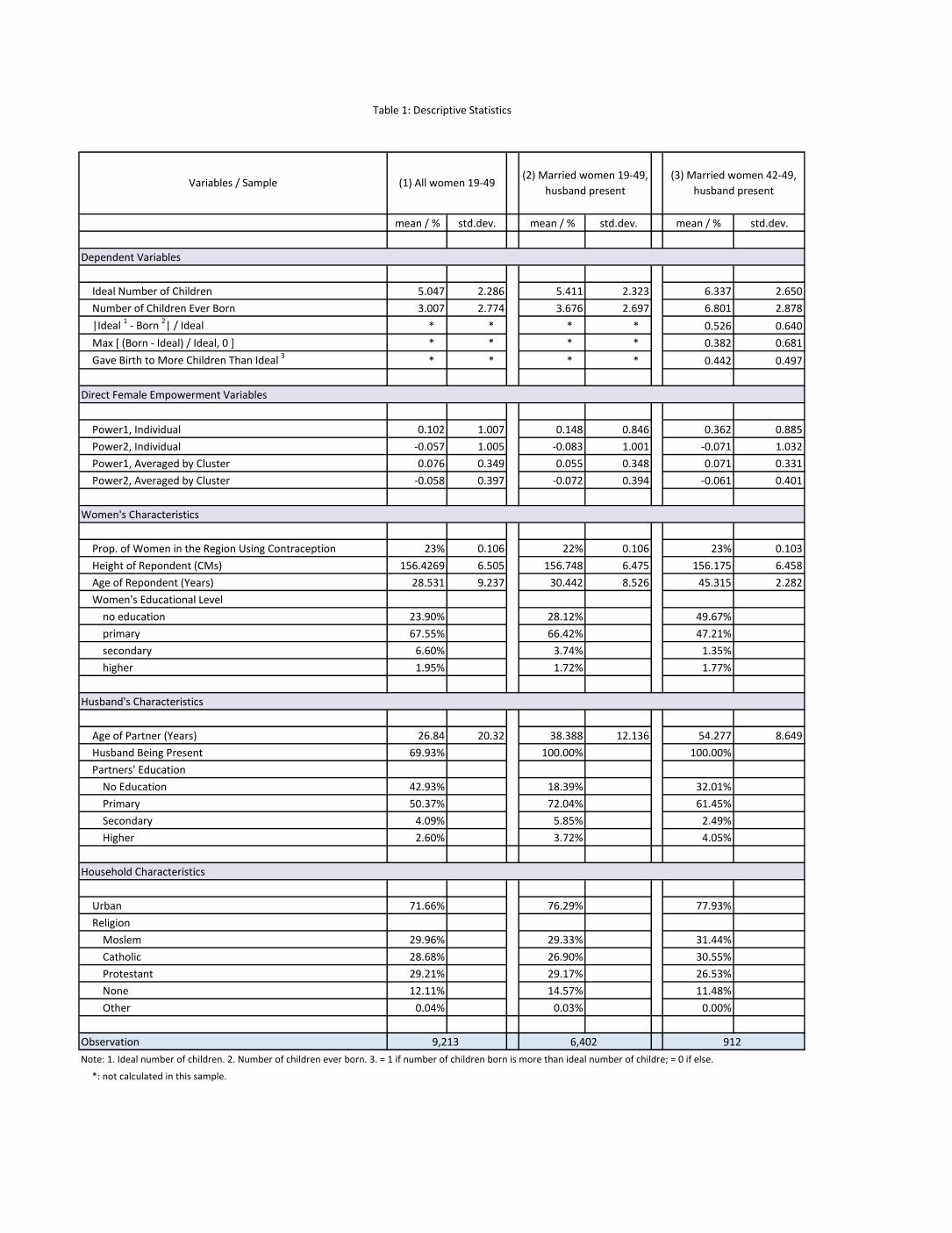
Table 1 shows the descriptive statistics of the three samples mentioned above. As shown, in

sample (1), the average ideal number of children is 5.36, with standard deviation of 2.44. The

sample (2) has a higher mean ideal number of children, 5.69 children on average and higher

number of children ever born. Sample (3) has much higher number of children ever born; this is

explained by the fact that respondents in sample (1) and (2) did not finish their reproductive

cycle. However, on average, women in sample (3) also prefer more children. From the mean of

DIFFERENCE variable |XYZ[\]^_`a|]^_`a in sample (3), we can see that on average the gap between

ideal and number of children ever born is around 50% of ideal number of children. In addition,

about 44% of respondents in sample (3) gave birth to more children than their desirable level.

Individual power 1 and 2 variables have mean zero and standard deviation of 1. As mentioned

above, the reason to use the sample of married women is that in this sample individual power

variables reflect relative power of women in domestic decision making and domestic violence

Page | 14

compared to their husbands, since daughter, mother, sister, etc. have been excluded from the

sample. On average, women’s individual power 1 and 2 are higher among married respondents

than all; women age 42-49 are on average much more empowered than 19-49.

Under women’s characteristics, the mean and standard deviation of proportion of women using

contraceptive methods, height, age, and education are described. On average, 20% of women use

contraceptive methods. Among all the regions, Dar Es Salam, Arusha, Morogoro, Tanga, Mbeya,

Kilimanjaro, Lindi, and Ruvuma have contraceptive coverage of over 30%. Also, regions with

higher proportion of urban population tend to use contraception more. The lowest coverage is in

Pemba North and Zanzibar North, which is only 5%. In sample (1), around 25% of women do

not have any education; 62% have the highest educational level being primary school. Only 13%

have educational level of secondary schooling and higher. In sample (3) the older generation, the

educational level is even lower. Around half of the respondents have no education at all; only 7%

have secondary schooling and higher.

In the whole sample, around 70% of respondents have husband being present at home.

Husbands’ educational level in sample (1) is even lower than the women. About 44% of the

partners do not have any education. Only 9% have educational level of secondary schooling and

higher. However, in the older generation—sample (3), only 34% of the partners do not have

education, compared to 49% among women; 56% have primary schooling, while only 43% in the

female respondents. 75-80% of the households are from the urban area in our sample. Also,

Moslems account for the highest proportion—43%, 43% and 47% in the three samples,

respectively. Catholic and Protestant account for 20-25%, respectively. In the samples we used,

Moslem tends to have more children and lower female empowerment.

Page | 15

4. Results

4.1 Women’s Empowerment and Ideal Number of Children

Table 2 shows the impact on ideal number of children of the direct female empowerment

variables, as well as women, husbands, and households’ characteristics. Models 1-4 use the

sample of all women 19-49 years old, while models 5-8 use the married women 19-49, also

husband being present at home. As explain in the methodology section, we expect that the

impact of empowerment variables is bigger in the married sample. Since region dummies are

added in models 1-8, independent variables power 1 and 2 averaged by cluster only capture the

variation in each region.

The individual power 1 and 2 variables have significantly negative impact on the ideal number of

children. When individual power 1 index (decision-making index) increases 1 standard

deviation, on average the ideal number of children will decrease 0.109. The impact of individual

power 2 index (domestic violence index) is lower at -0.0879. In addition, power 1 and 2

averaged by cluster also have quite significant impact. Domestic decision making capacity seems

to have bigger influence than domestic violence. As we mentioned in the previous session, the

impact of direct empowerment is expected to be higher in models 5-8 than 1-4. It turns out to be

true for individual power 1. Education, which is one source and proxy of women’s

empowerment, has significantly negative impact on ideal number of children. From the result of

model 1, we can see that compared to no education, women who completed primary school on

average want 0.462 fewer children; also, ideal number of children decreases 0.727 and 1.3 on

average if secondary school is finished and has higher education, respectively. Similar patterns

are observed from models 2-8.

Page | 16

Ideal number of children is also significantly correlated with other women’s characteristics—

height and age. Often, height is used as a proxy for women’s fecundity. Therefore, model 1

shows that women who are more fertile tend to have higher ideal number of children. This might

be due to the fact that they have higher expectation to the number of children they have. Model 5

shows that before 62, the ideal number of children increases with age, indicating that young

generation of women wants fewer children. Since in our dataset all respondents are under age 50,

ideal number of children can be considered increase with age. The impact of husbands’

education and age shows similar patterns to the wives although the impact is smaller. On

average, compared to husbands with no education, women whose husbands completed primary

school want 0.434 fewer children; 0.606 and 0.727 fewer children respectively for husbands who

finish secondary education and higher (model 1).

In the household characteristics, all the explanatory variables including urban, religion, wealth

index, and region are significant. According to the results in model 1, women in urban area on

average desire 0.324 fewer children than in the rural area. Compared to Moslem, Catholics and

Protestants tend to desire fewer children. Also, women with no religion want higher number of

children. The impact of wealth index on ideal number of children also has very clear pattern: the

ideal number of children decreases when household wealth increases; ideal number of children

drops significantly after wealth index gets 60% percentile and higher. In addition, most of the

region dummies are significant. Therefore, the ideal number of children has clear regional

pattern.

4.2 Women’s Empowerment and Number of Children Ever Born

Table 3A and 3B show the impact of the same sets of explanatory variables on number of

children ever born. Table 3A is comparable to table 2 because it uses the same samples and

Page | 17

variables. Table 3B adds contraceptive variable—proportion of women in the region using

contraception except the respondent herself to test the impact of the availability of family

planning. The difference between models 17-20 and 21-24 is that the latter ones include regional

health, education, welfare indicators.

Models 9-16 show that power 1 variables do not have significant impact on number of children

ever born; this is saying that women’s domestic decision-making power does not reduce the

actual number of children they gave birth to, although the ideal number is significantly lowered.

Power 2 individual and averaged by cluster do have significant impact, although compared to the

results in table 2, this impact is about 40-50% less than the one on ideal number of children.

Women with higher educational level tend to have fewer children. Those who completed

primary, secondary school or higher education gave birth to significantly lower number of

children, compared to no education. By comparing the coefficients of female educational

attainment in table 2, we observe that in general, the impact of primary education on number of

children ever born is much lower than on ideal number of children; secondary education has

approximately same size of impact; the impact of higher education is around 25% bigger than on

ideal number of children.

Women’s height does not have significant impact on the number of children ever born. Number

of children increases as age goes up. Also, as husbands’ educational level increases, the number

of children ever born goes down. Compared to ideal number of children, the impact on number

of children ever born is much smaller. Husband’s education is sometimes considered as a proxy

for household income. On one hand, the income effect will increase the demand for children as a

normal good when income goes up; also, since the husbands usually do not devote time on child-

raising, higher education of the husband does not increase the opportunity cost of having

Page | 18

children. These two reasons support the positive relation. On the other hand, literatures indicate

the substitution of quantity by quality when income increases. In our models, on average, the

impact of husbands’ education is negative.

URBAN is significant in model 9-11, but not from 12 to 16. This is partly due to the inclusion of

region dummies, which absorb some of the variance in URBAN. This can be seen in table 3B, the

impact of URBAN gets bigger when region dummies are removed. Further, adding other

regional characteristics also lowers the coefficients of URBAN. Thus, the impact of URBAN in

models 17-20 absorbs some of the influence of regional characteristics. Religion does not show

any significant impact on the number of children ever born. Therefore, although Catholic and

Protestant desire to have fewer children than Moslem, they are not capable to accomplish this

preference. Wealth index lowers the number of children ever born significantly. While wealth

index 20-60 percentile has approximately the same size of impact on number of children ever

born and ideal level, 60-100 percentile has obvious smaller coefficients in table 3A than table 2.

Therefore, compared to the poorest 20% of households, 20-60 percentile wealth level families

can well achieve their desire of fewer children; however, for the richest 40% families, the gap

between ideal and actual number of children born was broadened, since these families prefer a

much smaller family size.

Table 3B shows the impact of availability of contraceptive use on the number of children ever

born. The accessibility of contraception does significantly reduce number of children ever born.

By comparing the models with (21-24) and without (17-20) regional education, health and

welfare variables, we can see that the coefficients decreased dramatically in the models with

regional characteristics control. Thus, the impact of availability of contraception in models 17-20

Page | 19

absorbs the influence of other unobserved regional variables that affect fertility also (for

instance, region with higher contraception coverage is also better developed).

4.3 Women’s Empowerment, the Difference between Ideal and Actual Number of Children

Born, and Having More Children than Wanted

Models 25 to 32 in Table 4 mainly concentrate on the relationship between women’s

empowerment and the DIF F ERENCE variables. Generally, power 1 and 2 variables do not have

impact on DIFFERENCE. This is consistent with the results in table 2 and 3A: power 1

dramatically reduces the number of children wanted but does not have impact on the number

born; therefore, the gap becomes slightly bigger for empowered women (see model 29). Similar

result is obtained for power 2. Although power 2 reduces number of children ever born, it lowers

the ideal level even more. As a result, power 2 does not significantly reduce the gap between

ideal and actual number of children born. The only significance shown is power 1 averaged by

cluster in model 31. As direct female empowerment 1, women’s education also increases the gap

between ideal and actual number of children born, although the coefficients are not significant.

Respondents’ height does significantly reduce this gap in models 25-28. Since height is a proxy

for fecundity, this relationship can be explained by the fact that taller women have more capacity

to achieve the family size they wanted when what ideal number of children is higher than what

they actually had. For this reason, when only the amount that born is more than ideal is

considered (models 29-32), height does not transfer into a smaller gap. Husbands’ primary

education significantly increases the DIFFERENCE in models 27, and 29-32. But when it gets

the higher education level, the gap starts to drop. The same story happens to religion and wealth

index also. From models 29-32, we observe that the gap between ideal and actual number of

children born is bigger among Catholic and Protestant compared to Moslem, although Catholic

Page | 20

and Protestant want fewer children. Consistent with the fact that families with wealth index 60-

80 percentile desire 0.640 fewer children (model 5) than the poorest 20%, but they only managed

to reduce 0.460 in actual number born (model 13), the gap between ideal and actual number

increases significantly.

Results from the Probit model (table 5) further supports the previous conclusions. Table 5 shows

that direct female empowerment slightly increases the chance of having more children than

desired (in model 35, power 1 averaged by cluster significantly increases the likelihood of giving

birth to more). Also, both respondents and their husbands’ primary education have significantly

positive impact on having more children than wanted. This, again, reflects the results shown in

table 2 and 3: primary education has much bigger negative impact on ideal number of children

than actual number born. Therefore, empowerment actually increases the likelihood of giving

birth to more children than desired. Interestingly, wealth index has significantly negative impact

on having more children than wanted. This might be due to the fact that wealthier families have

better access to contraceptive methods.

5. Conclusion

Consistent with the second assumption at the beginning of the paper, ideal number of children is

not an unchanging target for women in Tanzania. As a matter of fact, women’s empowerment

defined in this paper, domestic decision-making ability, existence of domestic violence, and

education, reduces desirable fertility level dramatically. Unfortunately, very likely due to the

limited accessibility to other important resources, the enhancement of empowerment does not

affect actual number of children born as much. As a result, the gap between desirable and actual

fertility level has been broadened. On the other hand, the good news from this paper is although

Page | 21

actual fertility level has not dramatically decreased, women in Tanzania started to have the desire

of having smaller family size already, which is a necessary condition for fertility going down.

The same story repeats when comparing different religious groups, and households with different

wealth index.

As mentioned in the previous paragraph, the asymmetry is very likely due to the constraint of

some important resources. As a matter of fact, the most possible reason is the lack of

accessibility to contraception. As we mentioned in the introduction, less than 30% of women

surveyed were using some type of contraception, which is still considered really low. Also, the

fact that respondents in wealthier families (they have higher chance to get access to

contraception since there is less economic constraint) tend to be less likely to have more children

than they wanted indirectly supports the assumption that contraceptive availability is the main

obstacle in dropping fertility to the desirable level.

The limitation of the paper includes, first, contraception being the main constraint of achieving

desirable fertility is still an assumption, which is not empirically tested. Second, empowerment,

including education can be endogenous. Because this paper does not find appropriate

Instrumental Variables, the results got from the empirical analysis cannot be interpreted as causal

relationships.

Page | 22

Reference

Alexis Leon, (2004). “The Effect of Education on Fertility: Evidence from Compulsory Schooling Laws”, Department of Economics Working Papers #288, University of Pittsburgh. Retrieved from: http://www.pitt.edu/~aleon/papers/fertility.pdf

Anastasia J. Gage, (1995). “Women’s Socioeconomic Position and Contraceptive Behavior in Togo”. Studies in Family Planning, Vol. 26, No.5, pp. 264-277

Arkes, J. (2004).“Does Schooling Improve Adult Health?” Working Paper, RAND Corporation

Barbara L. Wolfe and Jere R. Behrman, (1987). “Women’s Schooling and Children’s Health: Are the Effects Robust with Adult Sibling Control for the Women’s Childhood Background?” Journal of Health Economics, 6(1987) 239-254.

De Walque, D., (2007). “Does Education Affect Smoking Behavior? Evidence Using the Vietnam Draft as an Instrument for College Education”. Journal of Health Economics 26:877-895

Deborah Balk, (1994). “Individual and Community Aspects of Women’s Status and Fertility in Rural Bangladesh”. Population Studies, Vol. 48, No.1, pp. 21-45

Dennis P. Hogan, Betemariam Berhanu, Assefa Hailemariam, (1999). “Household Organization, Women’s Autonomy, and Contraceptive Behavior in Southern Ethiopia”. Studies in Family Planning, Vol. 30, No.4, pp. 302-314

Gary S. Becker, “An Economic Analysis of fertility” in National Bureau of Economic Research, ed., Demographic and Economic Change in Developed Countries—A Conference of the University—National Bureau Committee for Economic Research, Princeton: Princeton University Press, 1960, pp.209-240

Getu Degu Alene and Alemayehu Worku, (2008). “Differentials of Fertility in North and South Gondar Zones, Northwest Ethiopia: A Comparative Cross-sectional Study”. BMC Public Health, 2008, 8:397

Jere R. Behrman, and Narbara L. Wolfe, (1987). “How Does Mother’s Schooling Affect Family Health, Nutrition, Medical Care Usage, and Household Sanitation?” Journal of Econometrics, 36(1987) 185-204

John Strauss, (1995). “Human Resources: Empirical Modeling of Household and Family Decisions”. Chapter 34, Handbook of Development Economics, Volume III, Edited by J. Behrman and T. N. Srinivasan, Elsvier Science B.V., 1995

Justin McCrary and Heather Royer, (2006). “The Effect of Female Education on Fertility and infant Health: Evidence from School Entry Policies Using Exact Date of Birth”. NBER Working Paper 12329. Retrieved from: http://www.nber.org/papers/w12329

Karen Oppenheim Mason, (1995). “Gender and Demographic Change: What Do We Know?” Location: International Union for the Scientific Study of Population (IUSSP).

Kofi Benefo and T. Paul Schultz, (1996). “Fertility and Child Mortality in Cote d’lvoire and Ghana”, The World Bank Economic Review, Vol.10, No.1, pp.123-158

http://www.nber.org/papers/w12329

http://www.pitt.edu/~aleon/papers/fertility.pdf

Page | 23

Lucia Breierova, and Esther Duflo, (2004)“The Impact of Education on Fertility and Child Mortality: Do Fathers Really Matter Less than Mothers?” NBER Working Paper 10513. Retrieved from: http://www.nber.org/papers/w10513

Marida Hollos, (1991). “Migration, Education, and the Status of Women in Southern Nigeria”. American Anthropologist, New Series, Vol. 93, No. 4

Mark R. Rosenzweig and T. Paul Schultz, “Schooling, Information and Nonmarket Productivity: Contraceptive Use and Its Effectiveness,” International Economic Review, May 1989, 30 (2), 457–477.

Marcel Fulop, (1977). “The Empirical Evidence from the Fertility Demand Functions: A Review of the Literature”. The American Economist, Vol.21, No.2, Fall, 1977

Ministry of Education & Vocational Training, United Republic of Tanzania, 2005, “Basic Education Statistics in Tanzania, Regional 2005”. Retrieved from http://216.15.191.173/statistics.html

Ministry of Health and Social Welfare, United Republic of Tanzania, 2006, “Annual Health Statistical Abstract”. Retrieved from http://www.moh.go.tz/documents/Abstract_2006_Version%203.pdf

Naila Kabeer, (2002). “Resources, Agency, Achievements: Reflections on the Measurement of Women’s Empowerment”. Sida studies No. 3. (ISBN 91-586-8957-5.) Retrieved from: http://www.sida.se/shared/jsp/download.jsp?f=SidaStudies+No3.pdf&a=2080

Ross E. J. Kinemo, “Abortion and Family Planning in Tanzania”. Retrieved from: http://www.tzonline.org/pdf/abortionandfamilyplanninintanzania.pdf

Sandra E. Black, Paul J. Devereux, and Kjell G. Salvanes, (2004). “Fast Times at Ridgemont High? The Effect of Compulsory Schooling Laws on Teenage Births”. NBER Working Paper 10911. Retrieved from: http://www.nber.org/papers/w10911

Sathar, Z.A., and S. Kazi, (1997). “Women’s Autonomy, Livelihood and Fertility. A Study of Rural Punjab ”. Islamabad, Pakistan Institute of Development Studies

Sidney Ruth Schuler and Syed M. Hashemi, (1994). “Credit Programs, Women’s Empowerment, and Contraceptive Use in Rural Bangladesh”. Studies in Family Planning, Vol.25, No.2, pp.65-76

Simon Appleton, (1996). “How Does Female Education Affect Fertility? A Structural Model for the Cote D’iviore”. Oxford Bulletin of Economics and Statistics, 58, 1(1996)

S. Philip Morgan and Bhanu b. Niraula, (1995). “Gender Inequality and Fertility in Two Nepali Villages”. Population and Development Review, Vol. 21, No. 3, pp. 541-561

Shin-Yi Chou, Jin-Tan Liu, Michael Grossman, and Theodore J. Joyce, (2007) “Parental Education and Child Health: Evidence from a Natural Experiment in Taiwan”. NBER Working Paper 13466. Retrieved from: http://www.nber.org/papers/w13466

T. Paul Schultz, (1994). “Human Capital, Family Planning, and Their Effects on Population Growth”. American Economic Review, 84(2), 225-260

http://www.sida.se/shared/jsp/download.jsp?f=SidaStudies+No3.pdf&a=2080

http://216.15.191.173/statistics.html

http://www.moh.go.tz/documents/Abstract_2006_Version%203.pdf

Page | 24

T. Paul Schultz, (2001). “The Fertility Transition: Economic Explanations”. Economic Growth Center Discussion Paper No.833. Retrieved from: http://papers.ssrn.com/abstract=286291

T. Paul Schultz, (2005). “Fertility and Income”, Economic Growth Center Discussion Paper No.925. Retrieved from: http://ssrn.com/abstract=838227

T. Paul Schultz, (2007). “Population Policies, Fertility, Women’s Human Capital, and Child Quality”. Economic Growth Center Discussion Paper No.954. Retrieved from: http://ssrn.com/abstract=985956

Ulla Larsen, and Marida Hollos, (2003). “Women’s Empowerment and Fertility Decline among the Pare of Kilimanjaro region, Northern Tanzania”. Social Science & Medicine, 57 (2003) 1099-1115

Una Okonkwo Osili, Bridget Terry Long, (2007). “Does Female Schooling Reduce Fertility? Evidence from Nigeria”. NBER Working Paper 13070. Retrieved from: http://www.nber.org/papers/w13070

http://ssrn.com/abstract=985956

http://papers.ssrn.com/abstract=286291

http://ssrn.com/abstract=838227

mean / % std.dev. mean / % std.dev. mean / % std.dev.

Ideal Number of Children 5.047 2.286 5.411 2.323 6.337 2.650Number of Children Ever Born 3.007 2.774 3.676 2.697 6.801 2.878|Ideal 1 ‐ Born 2| / Ideal * * * * 0.526 0.640Max [ (Born ‐ Ideal) / Ideal, 0 ] * * * * 0.382 0.681Gave Birth to More Children Than Ideal 3 * * * * 0.442 0.497

Power1, Individual 0.102 1.007 0.148 0.846 0.362 0.885Power2, Individual ‐0.057 1.005 ‐0.083 1.001 ‐0.071 1.032Power1, Averaged by Cluster 0.076 0.349 0.055 0.348 0.071 0.331Power2, Averaged by Cluster ‐0.058 0.397 ‐0.072 0.394 ‐0.061 0.401

Prop. of Women in the Region Using Contraception 23% 0.106 22% 0.106 23% 0.103Height of Repondent (CMs) 156.4269 6.505 156.748 6.475 156.175 6.458Age of Repondent (Years) 28.531 9.237 30.442 8.526 45.315 2.282Women's Educational Level no education 23.90% 28.12% 49.67% primary 67.55% 66.42% 47.21% secondary 6.60% 3.74% 1.35% higher 1.95% 1.72% 1.77%

Age of Partner (Years) 26.84 20.32 38.388 12.136 54.277 8.649Husband Being Present 69.93% 100.00% 100.00%Partners' Education No Education 42.93% 18.39% 32.01% Primary 50.37% 72.04% 61.45% Secondary 4.09% 5.85% 2.49% Higher 2.60% 3.72% 4.05%

Urban 71.66% 76.29% 77.93%Religion Moslem 29.96% 29.33% 31.44% Catholic 28.68% 26.90% 30.55% Protestant 29.21% 29.17% 26.53% None 12.11% 14.57% 11.48% Other 0.04% 0.03% 0.00%

Note: 1. Ideal number of children. 2. Number of children ever born. 3. = 1 if number of children born is more than ideal number of childre; = 0 if else.

*: not calculated in this sample.

(1) All women 19‐49

Household Characteristics

(3) Married women 42‐49, husband present

Variables / Sample

Table 1: Descriptive Statistics

(2) Married women 19‐49, husband present

Dependent Variables

Direct Female Empowerment Variables

Observation 9,213 6,402 912

Women's Characteristics

Husband's Characteristics

1 2 3 4 5 6 7 8


Power1, Individual ‐0.109*** ‐0.212***

(0.026) (0.037)

Power2, Individual ‐0.0879*** ‐0.0815***

(0.023) (0.029)

Power1, Averaged by Cluster ‐0.516*** ‐0.488***

(0.076) (0.097)

Power2, Averaged by Cluster ‐0.319*** ‐0.350***

(0.081) (0.102)


Educ. Primary ‐0.462*** ‐0.469*** ‐0.456*** ‐0.463*** ‐0.474*** ‐0.492*** ‐0.478*** ‐0.485***

(0.063) (0.063) (0.063) (0.063) (0.072) (0.072) (0.072) (0.072)

Educ. Secondary ‐0.727*** ‐0.689*** ‐0.718*** ‐0.700*** ‐0.751*** ‐0.754*** ‐0.766*** ‐0.767***

(0.093) (0.093) (0.093) (0.093) (0.130) (0.130) (0.129) (0.129)

Educ. Higher ‐1.300*** ‐1.259*** ‐1.302*** ‐1.278*** ‐1.287*** ‐1.295*** ‐1.334*** ‐1.316***

(0.114) (0.114) (0.115) (0.114) (0.154) (0.154) (0.155) (0.154)

Height 0.00933*** 0.00944*** 0.00858** 0.00917*** 0.0138*** 0.0139*** 0.0125*** 0.0137***

(0.004) (0.004) (0.004) (0.004) (0.004) (0.004) (0.004) (0.004)

Age 0.0399** 0.02 0.0221 0.0208 0.107*** 0.0988*** 0.0990*** 0.102***

(0.018) (0.018) (0.018) (0.018) (0.027) (0.027) (0.027) (0.027)

Age Square 0.000253 0.000465 0.000435 0.000452 ‐0.000870** ‐0.000797* ‐0.000802** ‐0.000834**

(0.000) (0.000) (0.000) (0.000) (0.000) (0.000) (0.000) (0.000)


Husban's Educ. Primary * Present_husband ‐0.434*** ‐0.438*** ‐0.413*** ‐0.438*** ‐0.420*** ‐0.425*** ‐0.401*** ‐0.425***

(0.088) (0.088) (0.088) (0.088) (0.089) (0.089) (0.089) (0.090)

Husban's Educ. Secondary * Present_husband ‐0.606*** ‐0.620*** ‐0.591*** ‐0.630*** ‐0.562*** ‐0.579*** ‐0.562*** ‐0.583***

(0.120) (0.121) (0.121) (0.121) (0.127) (0.127) (0.127) (0.127)

Husban's Educ. Higher * Present_husband ‐0.727*** ‐0.758*** ‐0.739*** ‐0.763*** ‐0.678*** ‐0.712*** ‐0.703*** ‐0.710***

(0.132) (0.132) (0.133) (0.133) (0.143) (0.143) (0.144) (0.144)

Age of Husband 0.0239** 0.0324*** 0.0310*** 0.0325*** 0.0267** 0.0262** 0.0255* 0.0251*

(0.011) (0.011) (0.011) (0.011) (0.013) (0.013) (0.013) (0.013)

Age of Husband, Square ‐0.000194* ‐0.000265** ‐0.000248** ‐0.000266** ‐1.78E‐04 ‐1.81E‐04 ‐1.71E‐04 ‐1.74E‐04

(0.000) (0.000) (0.000) (0.000) (0.000) (0.000) (0.000) (0.000)

Presnet_husband 0.236 0.0691 0.0711 0.0634

(0.274) (0.268) (0.267) (0.267)


Urban ‐0.324*** ‐0.333*** ‐0.298*** ‐0.298*** ‐0.334*** ‐0.351*** ‐0.317*** ‐0.317***

(0.056) (0.056) (0.056) (0.057) (0.071) (0.071) (0.071) (0.072)

Religion = Catholic ‐0.265*** ‐0.267*** ‐0.242*** ‐0.262*** ‐0.301*** ‐0.318*** ‐0.290*** ‐0.312***

(0.058) (0.058) (0.058) (0.058) (0.076) (0.076) (0.076) (0.076)

Religion = Protestant ‐0.217*** ‐0.217*** ‐0.212*** ‐0.218*** ‐0.228*** ‐0.234*** ‐0.233*** ‐0.240***

(0.059) (0.059) (0.059) (0.059) (0.076) (0.076) (0.076) (0.076)

Religion = None 0.789*** 0.818*** 0.732*** 0.833*** 0.784*** 0.833*** 0.763*** 0.851***

(0.122) (0.124) (0.123) (0.123) (0.140) (0.142) (0.141) (0.141)

Religion = Others ‐1.672* ‐1.611* ‐1.795** ‐1.569* ‐2.826*** ‐2.693*** ‐2.895*** ‐2.658***

(0.898) (0.865) (0.851) (0.874) (0.821) (0.818) (0.719) (0.812)

wealthindex, 20‐40% ‐0.228*** ‐0.222*** ‐0.217*** ‐0.215*** ‐0.231** ‐0.228** ‐0.220** ‐0.218**

(0.079) (0.079) (0.079) (0.079) (0.095) (0.095) (0.095) (0.096)

wealthindex, 40‐60% ‐0.236*** ‐0.227*** ‐0.211*** ‐0.216*** ‐0.289*** ‐0.287*** ‐0.269*** ‐0.272***

(0.078) (0.078) (0.078) (0.078) (0.093) (0.093) (0.093) (0.094)

wealthindex, 60‐80% ‐0.582*** ‐0.572*** ‐0.548*** ‐0.555*** ‐0.640*** ‐0.643*** ‐0.617*** ‐0.624***

(0.076) (0.076) (0.076) (0.076) (0.093) (0.094) (0.094) (0.094)

wealthindex, 80‐100% ‐0.928*** ‐0.907*** ‐0.888*** ‐0.878*** ‐0.976*** ‐0.978*** ‐0.949*** ‐0.941***

(0.087) (0.088) (0.087) (0.088) (0.111) (0.111) (0.111) (0.112)

Region = Arusha ‐0.0117 ‐0.0222 ‐0.0653 ‐0.0484 0.0263 0.0115 ‐0.0205 ‐0.0292

(0.131) (0.131) (0.131) (0.130) (0.163) (0.165) (0.164) (0.162)

Region = Kilimanjaro ‐0.206* ‐0.169 ‐0.146 ‐0.0633 0.0202 ‐0.0115 0.0276 0.128

(0.124) (0.124) (0.124) (0.130) (0.153) (0.153) (0.153) (0.161)

Region = Tanga 0.0402 0.0511 0.0963 0.0592 0.232 0.221 0.265 0.231

(0.138) (0.138) (0.137) (0.137) (0.167) (0.167) (0.167) (0.167)

Region = Morogoro 0.513*** 0.558*** 0.495*** 0.619*** 0.673*** 0.733*** 0.696*** 0.807***

(0.139) (0.140) (0.140) (0.142) (0.169) (0.172) (0.172) (0.173)

Region = Pwani 0.887*** 0.964*** 0.807*** 1.071*** 1.076*** 1.170*** 1.035*** 1.293***

(0.160) (0.161) (0.161) (0.164) (0.183) (0.186) (0.186) (0.190)

Region = Dar es salam 0.205 0.213 0.205 0.241* 0.461*** 0.443** 0.449** 0.470***

(0.133) (0.133) (0.133) (0.133) (0.177) (0.178) (0.178) (0.178)

Region = Lindi 0.225 0.268* 0.18 0.307** 0.259 0.330* 0.25 0.370**

(0.143) (0.143) (0.142) (0.144) (0.169) (0.171) (0.169) (0.171)

Region = Mtwara ‐0.404*** ‐0.348** ‐0.488*** ‐0.324** ‐0.224 ‐0.131 ‐0.263 ‐0.0984

(0.135) (0.135) (0.136) (0.135) (0.164) (0.166) (0.166) (0.166)

Region = Ruvuma 0.377*** 0.399*** 0.269* 0.352** 0.528*** 0.590*** 0.453*** 0.521***

Table 2: The Impact of Women's Empowerment on Ideal Number of Children, OLS

Ideal Number of Children

Sample All women 19‐49 Married women 19‐49, husband present

ModelDependent Variable

(0.137) (0.137) (0.138) (0.137) (0.160) (0.160) (0.162) (0.162)

Region = Iringga ‐0.0433 ‐0.0737 0.0284 ‐0.136 ‐0.0137 ‐0.0573 0.0331 ‐0.138

(0.126) (0.126) (0.125) (0.127) (0.150) (0.151) (0.150) (0.152)

Region = Mbeya 0.365*** 0.376*** 0.448*** 0.447*** 0.578*** 0.566*** 0.637*** 0.649***

(0.138) (0.138) (0.138) (0.140) (0.159) (0.160) (0.161) (0.163)

Region = Singida 0.405*** 0.407*** 0.401*** 0.399*** 0.547*** 0.553*** 0.540*** 0.553***

(0.140) (0.140) (0.140) (0.140) (0.168) (0.168) (0.168) (0.168)

Region = Tabora 0.654*** 0.684*** 0.483*** 0.637*** 0.718*** 0.804*** 0.612*** 0.750***

(0.144) (0.144) (0.148) (0.145) (0.168) (0.168) (0.174) (0.169)

Region = Rukwa 1.094*** 1.105*** 1.161*** 1.174*** 1.266*** 1.260*** 1.319*** 1.342***

(0.188) (0.189) (0.187) (0.188) (0.225) (0.227) (0.225) (0.226)

Region = Kigoma 1.833*** 1.828*** 1.675*** 1.722*** 1.987*** 2.005*** 1.861*** 1.887***

(0.147) (0.148) (0.150) (0.151) (0.175) (0.176) (0.179) (0.181)

Region = Shinyanga 0.629*** 0.665*** 0.472*** 0.655*** 0.717*** 0.803*** 0.629*** 0.795***

(0.148) (0.148) (0.151) (0.148) (0.173) (0.173) (0.177) (0.173)

Region = Kagera 0.378*** 0.451*** 0.305** 0.551*** 0.475*** 0.594*** 0.463*** 0.708***

(0.133) (0.134) (0.134) (0.137) (0.152) (0.154) (0.154) (0.159)

Region = Mwanza 0.666*** 0.710*** 0.676*** 0.806*** 0.722*** 0.808*** 0.785*** 0.927***

(0.135) (0.135) (0.135) (0.138) (0.163) (0.164) (0.163) (0.167)

Region = Mara 0.876*** 0.831*** 0.862*** 0.721*** 0.809*** 0.819*** 0.857*** 0.684***

(0.164) (0.165) (0.163) (0.168) (0.193) (0.196) (0.194) (0.200)

Region = Manyara 0.417*** 0.399*** 0.441*** 0.362*** 0.461*** 0.422** 0.469*** 0.374**

(0.139) (0.139) (0.138) (0.139) (0.163) (0.164) (0.163) (0.164)

Region = Zanzibar North 1.688*** 1.804*** 1.504*** 1.933*** 1.630*** 1.813*** 1.555*** 1.952***

(0.173) (0.172) (0.178) (0.180) (0.206) (0.205) (0.211) (0.213)

Region = Zanzibar South 1.534*** 1.616*** 1.437*** 1.753*** 1.512*** 1.655*** 1.491*** 1.799***

(0.169) (0.169) (0.170) (0.174) (0.203) (0.205) (0.205) (0.209)

Region = Town west 1.376*** 1.466*** 1.220*** 1.594*** 1.390*** 1.554*** 1.339*** 1.696***

(0.150) (0.150) (0.154) (0.156) (0.183) (0.182) (0.187) (0.189)

Region = Pemba North 3.102*** 3.230*** 2.856*** 3.399*** 3.191*** 3.415*** 3.070*** 3.613***

(0.173) (0.174) (0.178) (0.183) (0.223) (0.223) (0.226) (0.234)

Region = Pemba South 3.138*** 3.223*** 2.927*** 3.318*** 3.319*** 3.475*** 3.211*** 3.582***

(0.187) (0.187) (0.193) (0.193) (0.239) (0.237) (0.245) (0.245)

Constant 2.372*** 2.658*** 2.834*** 2.631*** 0.807 0.942 1.205 0.867

(0.605) (0.596) (0.591) (0.593) (0.756) (0.763) (0.757) (0.759)

Observations 9213 9213 9213 9213 6402 6402 6402 6402

R‐squared 0.339 0.339 0.340 0.338 0.306 0.303 0.304 0.303

Robust standard errors in parentheses

*** p<0.01, ** p<0.05, * p<0.1

9 10 11 12 13 14 15 16


Power1, Individual 0.0367 0.0161

(0.023) (0.032)

Power2, Individual ‐0.0454** ‐0.0501**

(0.019) (0.025)

Power1, Averaged by Cluster ‐0.0332 ‐0.111

(0.069) (0.090)

Power2, Averaged by Cluster ‐0.192*** ‐0.171*

(0.070) (0.091)


Educ. Primary ‐0.175*** ‐0.176*** ‐0.174*** ‐0.172*** ‐0.143** ‐0.145** ‐0.140** ‐0.141**

(0.054) (0.054) (0.054) (0.054) (0.063) (0.063) (0.063) (0.063)

Educ. Secondary ‐0.687*** ‐0.683*** ‐0.693*** ‐0.687*** ‐0.792*** ‐0.781*** ‐0.790*** ‐0.790***

(0.076) (0.076) (0.076) (0.076) (0.110) (0.110) (0.110) (0.110)

Educ. Higher ‐1.558*** ‐1.540*** ‐1.559*** ‐1.548*** ‐1.516*** ‐1.489*** ‐1.512*** ‐1.504***

(0.129) (0.129) (0.129) (0.129) (0.192) (0.191) (0.192) (0.191)

Height 0.00357 0.00393 0.00366 0.0038 0.00426 0.00462 0.0041 0.00448

(0.003) (0.003) (0.003) (0.003) (0.004) (0.004) (0.004) (0.004)

Age 0.254*** 0.262*** 0.261*** 0.262*** 0.363*** 0.363*** 0.363*** 0.365***

(0.017) (0.016) (0.016) (0.016) (0.022) (0.022) (0.022) (0.022)

Age Square ‐0.000891*** ‐0.000969*** ‐0.000967*** ‐0.000978*** ‐0.00225*** ‐0.00225*** ‐0.00226*** ‐0.00227***

(0.000) (0.000) (0.000) (0.000) (0.000) (0.000) (0.000) (0.000)


Husban's Educ. Primary * Present_husband ‐0.160** ‐0.157** ‐0.157** ‐0.157** ‐0.113 ‐0.111 ‐0.107 ‐0.111

(0.072) (0.072) (0.072) (0.072) (0.074) (0.074) (0.074) (0.074)

Husban's Educ. Secondary * Present_husband ‐0.243** ‐0.232** ‐0.233** ‐0.237** ‐0.199* ‐0.193* ‐0.192* ‐0.196*

(0.101) (0.101) (0.102) (0.101) (0.108) (0.108) (0.108) (0.108)


(0.140) (0.139) (0.140) (0.140) (0.155) (0.154) (0.154) (0.155)

Age of Husband 0.0991*** 0.0967*** 0.0964*** 0.0968*** 0.0580*** 0.0586*** 0.0582*** 0.0580***

(0.009) (0.009) (0.009) (0.009) (0.010) (0.010) (0.010) (0.010)

Age of Husband, Square ‐0.000834*** ‐0.000815*** ‐0.000812*** ‐0.000817*** ‐0.000495*** ‐0.000500*** ‐0.000495*** ‐0.000496***

(0.000) (0.000) (0.000) (0.000) (0.000) (0.000) (0.000) (0.000)

present_husband ‐1.517*** ‐1.476*** ‐1.468*** ‐1.481***

(0.193) (0.192) (0.192) (0.192)


Urban ‐0.103** ‐0.0959* ‐0.0958* ‐0.0746 ‐0.111 ‐0.107 ‐0.101 ‐0.0909

(0.052) (0.052) (0.052) (0.053) (0.070) (0.070) (0.070) (0.071)

Religion = Catholic 0.0629 0.0674 0.0671 0.071 0.00809 0.0128 0.0172 0.015

(0.054) (0.054) (0.054) (0.054) (0.073) (0.072) (0.072) (0.072)

Religion = Protestant 0.0435 0.0484 0.0462 0.0481 0.0315 0.0385 0.0351 0.0346

(0.054) (0.054) (0.054) (0.054) (0.072) (0.072) (0.072) (0.072)

Religion = None ‐0.0824 ‐0.082 ‐0.0929 ‐0.072 ‐0.0339 ‐0.0298 ‐0.0501 ‐0.0222

(0.091) (0.091) (0.092) (0.091) (0.107) (0.107) (0.108) (0.108)

Religion = Others ‐0.103 ‐0.112 ‐0.13 ‐0.0856 ‐0.805 ‐0.784 ‐0.847 ‐0.772

(0.623) (0.615) (0.626) (0.621) (0.494) (0.504) (0.521) (0.505)

wealthindex, 20‐40% ‐0.245*** ‐0.247*** ‐0.247*** ‐0.243*** ‐0.255*** ‐0.256*** ‐0.254*** ‐0.251***

(0.062) (0.062) (0.062) (0.062) (0.076) (0.076) (0.075) (0.076)

wealthindex, 40‐60% ‐0.336*** ‐0.338*** ‐0.337*** ‐0.331*** ‐0.335*** ‐0.333*** ‐0.330*** ‐0.326***

(0.066) (0.066) (0.066) (0.066) (0.081) (0.081) (0.081) (0.081)

wealthindex, 60‐80% ‐0.407*** ‐0.405*** ‐0.406*** ‐0.395*** ‐0.460*** ‐0.455*** ‐0.452*** ‐0.447***

(0.066) (0.066) (0.066) (0.066) (0.084) (0.084) (0.084) (0.084)

wealthindex, 80‐100% ‐0.694*** ‐0.689*** ‐0.694*** ‐0.670*** ‐0.823*** ‐0.813*** ‐0.812*** ‐0.797***

(0.075) (0.075) (0.075) (0.076) (0.100) (0.100) (0.101) (0.102)

Region = Arusha ‐0.0725 ‐0.082 ‐0.0779 ‐0.0991 ‐0.0657 ‐0.0759 ‐0.0768 ‐0.0938

(0.105) (0.106) (0.106) (0.106) (0.139) (0.140) (0.140) (0.140)

Region = Kilimanjaro ‐0.258** ‐0.231* ‐0.251** ‐0.163 ‐0.380** ‐0.349** ‐0.356** ‐0.286

(0.120) (0.121) (0.121) (0.124) (0.169) (0.169) (0.169) (0.175)

Region = Tanga ‐0.405*** ‐0.400*** ‐0.402*** ‐0.395*** ‐0.576*** ‐0.566*** ‐0.561*** ‐0.563***

(0.125) (0.125) (0.125) (0.125) (0.161) (0.161) (0.161) (0.161)

Region = Morogoro ‐0.346*** ‐0.340*** ‐0.355*** ‐0.301** ‐0.397** ‐0.388** ‐0.404** ‐0.355**

(0.124) (0.124) (0.124) (0.125) (0.161) (0.161) (0.160) (0.162)

Region = Pwani ‐0.387*** ‐0.374*** ‐0.405*** ‐0.306** ‐0.485*** ‐0.459*** ‐0.509*** ‐0.405**

(0.131) (0.131) (0.132) (0.134) (0.168) (0.168) (0.169) (0.172)

Region = Dar es salam ‐0.462*** ‐0.457*** ‐0.461*** ‐0.439*** ‐0.625*** ‐0.613*** ‐0.618*** ‐0.602***

(0.111) (0.111) (0.111) (0.111) (0.152) (0.152) (0.152) (0.152)

Table 3A: The Impact of Women's Empowerment on Number of Children Ever Born, OLS

ModelDependent Variable Number of Children Ever Born

Sample All women 19‐49 Married women 19‐49, husband present

Region = Lindi ‐0.548*** ‐0.546*** ‐0.561*** ‐0.521*** ‐0.828*** ‐0.817*** ‐0.844*** ‐0.800***

(0.124) (0.125) (0.125) (0.124) (0.159) (0.159) (0.159) (0.159)

Region = Mtwara ‐0.789*** ‐0.795*** ‐0.810*** ‐0.779*** ‐1.062*** ‐1.053*** ‐1.092*** ‐1.040***

(0.124) (0.124) (0.125) (0.124) (0.159) (0.159) (0.160) (0.159)

Region = Ruvuma ‐0.0453 ‐0.067 ‐0.0679 ‐0.0972 ‐0.135 ‐0.143 ‐0.173 ‐0.176

(0.110) (0.110) (0.112) (0.111) (0.144) (0.143) (0.146) (0.145)

Region = Iringga ‐0.317*** ‐0.328*** ‐0.310*** ‐0.368*** ‐0.351** ‐0.356** ‐0.331** ‐0.394***

(0.111) (0.111) (0.111) (0.113) (0.148) (0.148) (0.148) (0.151)

Region = Mbeya 0.157 0.177 0.169 0.222* 0.241 0.261* 0.267* 0.299**

(0.122) (0.122) (0.122) (0.123) (0.148) (0.149) (0.149) (0.150)

Region = Singida ‐0.190* ‐0.197* ‐0.194* ‐0.203* ‐0.18 ‐0.185 ‐0.185 ‐0.185

(0.113) (0.113) (0.113) (0.113) (0.148) (0.148) (0.148) (0.148)

Region = Tabora 0.146 0.117 0.114 0.0865 0.155 0.139 0.1 0.114

(0.117) (0.117) (0.120) (0.117) (0.145) (0.144) (0.149) (0.145)

Region = Rukwa 0.337*** 0.357*** 0.348*** 0.401*** 0.469*** 0.493*** 0.493*** 0.529***

(0.123) (0.123) (0.123) (0.124) (0.149) (0.149) (0.150) (0.151)

Region = Kigoma 0.464*** 0.426*** 0.438*** 0.358*** 0.670*** 0.640*** 0.623*** 0.587***

(0.115) (0.115) (0.118) (0.120) (0.151) (0.151) (0.154) (0.157)

Region = Shinyanga 0.355*** 0.337*** 0.328*** 0.331*** 0.437*** 0.429*** 0.390*** 0.425***

(0.124) (0.123) (0.126) (0.123) (0.147) (0.146) (0.150) (0.146)

Region = Kagera 0.334*** 0.343*** 0.316*** 0.407*** 0.343** 0.363** 0.317** 0.413***

(0.120) (0.120) (0.121) (0.123) (0.145) (0.145) (0.145) (0.148)

Region = Mwanza 0.269** 0.286** 0.267** 0.347*** 0.248 0.266* 0.247 0.320**

(0.121) (0.122) (0.122) (0.123) (0.159) (0.159) (0.159) (0.161)

Region = Mara 0.425*** 0.390*** 0.418*** 0.318** 0.450*** 0.414*** 0.442*** 0.355**

(0.128) (0.129) (0.129) (0.134) (0.157) (0.158) (0.157) (0.166)

Region = Manyara 0.0367 0.025 0.037 0.000676 0.0683 0.0603 0.0772 0.0387

(0.127) (0.127) (0.127) (0.127) (0.161) (0.162) (0.162) (0.162)

Region = Zanzibar North 0.666*** 0.672*** 0.629*** 0.754*** 0.902*** 0.925*** 0.845*** 0.986***

(0.149) (0.149) (0.154) (0.154) (0.192) (0.192) (0.196) (0.197)

Region = Zanzibar South 0.294** 0.304** 0.273** 0.391*** 0.312* 0.336* 0.279 0.400**

(0.138) (0.138) (0.139) (0.144) (0.176) (0.176) (0.177) (0.183)

Region = Town west ‐0.00381 ‐0.00169 ‐0.0347 0.0784 0.107 0.125 0.0593 0.189

(0.131) (0.131) (0.135) (0.135) (0.179) (0.178) (0.182) (0.184)

Region = Pemba North 0.547*** 0.562*** 0.507*** 0.669*** 0.858*** 0.888*** 0.783*** 0.976***

(0.129) (0.129) (0.136) (0.137) (0.175) (0.173) (0.182) (0.184)

Region = Pemba South 0.778*** 0.777*** 0.743*** 0.837*** 1.095*** 1.106*** 1.033*** 1.154***

(0.133) (0.133) (0.139) (0.136) (0.178) (0.177) (0.183) (0.181)

Constant ‐3.980*** ‐4.165*** ‐4.107*** ‐4.190*** ‐6.543*** ‐6.639*** ‐6.531*** ‐6.660***

(0.489) (0.482) (0.482) (0.483) (0.661) (0.659) (0.660) (0.662)

Observations 9213 9213 9213 9213 6402 6402 6402 6402

R‐squared 0.658 0.658 0.658 0.658 0.582 0.582 0.582 0.582


*** p<0.01, ** p<0.05, * p<0.1

17 18 19 20 21 22 23 24



(0.031) (0.032)

Power2, Individual ‐0.0466* ‐0.0580**

(0.024) (0.024)


(0.075) (0.082)

Power2, Averaged by Cluster ‐0.0585 ‐0.191**

(0.060) (0.076)


Prop. of Women in the Region Using Contraception ‐3.492*** ‐3.474*** ‐3.316*** ‐3.487*** ‐2.115*** ‐1.910*** ‐1.988*** ‐1.688***

(except the respondent herself) (0.233) (0.228) (0.244) (0.230) (0.453) (0.452) (0.476) (0.475)

Educ. Primary ‐0.201*** ‐0.206*** ‐0.198*** ‐0.203*** ‐0.165*** ‐0.166*** ‐0.162** ‐0.162**

(0.064) (0.064) (0.064) (0.064) (0.064) (0.063) (0.064) (0.063)

Educ. Secondary ‐0.738*** ‐0.725*** ‐0.741*** ‐0.732*** ‐0.854*** ‐0.842*** ‐0.850*** ‐0.856***

(0.106) (0.107) (0.106) (0.106) (0.110) (0.110) (0.110) (0.110)

Educ. Higher ‐1.518*** ‐1.494*** ‐1.520*** ‐1.512*** ‐1.560*** ‐1.525*** ‐1.552*** ‐1.543***

(0.191) (0.191) (0.191) (0.191) (0.192) (0.192) (0.192) (0.192)

Height 0.00669* 0.00692* 0.00680* 0.00672* 0.00545 0.00594 0.00563 0.0058

(0.004) (0.004) (0.004) (0.004) (0.004) (0.004) (0.004) (0.004)

Age 0.363*** 0.364*** 0.364*** 0.365*** 0.363*** 0.365*** 0.365*** 0.366***

(0.023) (0.023) (0.023) (0.023) (0.022) (0.022) (0.022) (0.022)

Age Square ‐0.00228*** ‐0.00229*** ‐0.00229*** ‐0.00230*** ‐0.00226*** ‐0.00227*** ‐0.00227*** ‐0.00229***

(0.000) (0.000) (0.000) (0.000) (0.000) (0.000) (0.000) (0.000)


Husban's Educ. Primary * Present_husband ‐0.164** ‐0.164** ‐0.155** ‐0.165** ‐0.138* ‐0.134* ‐0.135* ‐0.136*

(0.074) (0.074) (0.074) (0.074) (0.074) (0.074) (0.074) (0.074)

Husban's Educ. Secondary * Present_husband ‐0.148 ‐0.14 ‐0.142 ‐0.143 ‐0.238** ‐0.229** ‐0.232** ‐0.234**

(0.108) (0.108) (0.108) (0.108) (0.108) (0.108) (0.108) (0.108)


(0.156) (0.155) (0.156) (0.156) (0.157) (0.156) (0.156) (0.157)

Age of Husband 0.0577*** 0.0581*** 0.0578*** 0.0577*** 0.0568*** 0.0577*** 0.0571*** 0.0571***

(0.010) (0.010) (0.010) (0.010) (0.010) (0.010) (0.010) (0.010)

Age of Husband, Square ‐0.000476*** ‐0.000481*** ‐0.000475*** ‐0.000477*** ‐0.000485*** ‐0.000493*** ‐0.000486*** ‐0.000489***

(0.000) (0.000) (0.000) (0.000) (0.000) (0.000) (0.000) (0.000)


Urban ‐0.218*** ‐0.216*** ‐0.204*** ‐0.212*** ‐0.145** ‐0.139** ‐0.141** ‐0.122*

(0.069) (0.068) (0.068) (0.069) (0.070) (0.070) (0.070) (0.070)

Religion = Catholic 0.130** 0.128** 0.159** 0.126** 0.184*** 0.188*** 0.194*** 0.179***

(0.063) (0.062) (0.063) (0.063) (0.069) (0.069) (0.069) (0.069)

Religion = Protestant 0.209*** 0.206*** 0.233*** 0.201*** 0.236*** 0.244*** 0.246*** 0.230***

(0.060) (0.060) (0.061) (0.061) (0.066) (0.066) (0.066) (0.066)

Religion = None 0.0957 0.0876 0.0922 0.0854 0.164 0.158 0.158 0.154

(0.091) (0.091) (0.091) (0.092) (0.100) (0.100) (0.101) (0.100)

Religion = Others ‐0.509 ‐0.492 ‐0.549 ‐0.504 ‐0.511 ‐0.5 ‐0.529 ‐0.497

(0.709) (0.719) (0.731) (0.715) (0.597) (0.609) (0.604) (0.609)

wealthindex, 20‐40% ‐0.183** ‐0.181** ‐0.177** ‐0.179** ‐0.198*** ‐0.199*** ‐0.197*** ‐0.195***

(0.075) (0.075) (0.075) (0.076) (0.076) (0.076) (0.076) (0.076)

wealthindex, 40‐60% ‐0.190** ‐0.185** ‐0.185** ‐0.183** ‐0.267*** ‐0.264*** ‐0.265*** ‐0.256***

(0.080) (0.080) (0.080) (0.081) (0.081) (0.081) (0.081) (0.081)

wealthindex, 60‐80% ‐0.201** ‐0.190** ‐0.190** ‐0.189** ‐0.347*** ‐0.338*** ‐0.341*** ‐0.328***

(0.080) (0.080) (0.080) (0.081) (0.083) (0.082) (0.083) (0.083)

wealthindex, 80‐100% ‐0.622*** ‐0.607*** ‐0.606*** ‐0.605*** ‐0.760*** ‐0.746*** ‐0.752*** ‐0.726***

(0.096) (0.096) (0.097) (0.097) (0.099) (0.099) (0.100) (0.100)

Regional Characteristics

Classroom: Shortage / Required ‐0.25 ‐0.134 ‐0.231 0.0971

(0.606) (0.608) (0.610) (0.623)

Pupil ‐ Teacher Ratio 0.0342*** 0.0330*** 0.0342*** 0.0313***

(0.006) (0.006) (0.006) (0.006)

Prop. of Women with Body Mass Index of Less than 18.5 ‐2.472*** ‐2.366*** ‐2.324*** ‐2.395***

(0.782) (0.776) (0.792) (0.774)

Missing: Classroom Shortage, Pupil‐teacher Ratio, and Mass Index 2.838*** 2.791*** 2.847*** 2.737***

(0.411) (0.410) (0.412) (0.409)

Population Ratio per One Medical Doctor ‐0.243*** ‐0.214*** ‐0.233*** ‐0.175***

(0.047) (0.047) (0.048) (0.052)

Missing: Population Ratio per One Medical Doctor ‐0.301** ‐0.248** ‐0.289** (0.154)

Table 3B: The Impact of Women's Empowerment on Number of Children Ever Born, Contraceptive variable added, OLS

Model

Dependent Variable Number of Children Ever Born

Sample Married women 19‐49, husband present

(0.120) (0.121) (0.121) (0.129)

Prop. Of HHs with Safe Water Source 1.382*** 1.409*** 1.416*** 1.410***

(0.293) (0.292) (0.295) (0.292)

Missing: Prop. Of HHs with Safe Water Source 0.488** 0.524** 0.521** 0.535**

(0.221) (0.220) (0.222) (0.220)

Prop. Of HHs with Appropriate Latrines ‐0.137 ‐0.204 ‐0.177 ‐0.289

(0.265) (0.265) (0.271) (0.271)

Missing: Prop. Of HHs with Appropriate Latrines ‐0.744*** ‐0.736*** ‐0.776*** ‐0.680***

(0.252) (0.251) (0.254) (0.251)

Constant ‐6.276*** ‐6.352*** ‐6.375*** ‐6.318*** ‐8.144*** ‐8.351*** ‐8.279*** ‐8.432***

(0.653) (0.649) (0.650) (0.649) (0.721) (0.715) (0.721) (0.722)

Observations 6402 6402 6402 6402 6402 6402 6402 6402

R‐Squared 0.568 0.568 0.568 0.568 0.575 0.575 0.575 0.575


*** p<0.01, ** p<0.05, * p<0.1

25 26 27 28 29 30 31 32



(0.027) (0.050)

Power2, Individual ‐0.0121 ‐0.0543

(0.024) (0.044)

Power1, Averaged by Cluster ‐0.0755 0.278*

(0.094) (0.161)


(0.093) (0.140)


Prop. of Women in the Region Using Contraception ‐0.509 ‐0.286 ‐0.838 ‐0.0269

(except the respondent herself) (0.807) (0.803) (0.845) (0.830)

Educ. Primary 0.0183 0.0196 0.022 0.0197 0.13 0.132 0.134 0.14

(0.052) (0.052) (0.052) (0.052) (0.097) (0.097) (0.097) (0.097)

Educ. Secondary ‐0.0785 ‐0.0714 ‐0.0742 ‐0.0757 0.0688 0.0921 0.095 0.0729

(0.118) (0.117) (0.117) (0.117) (0.218) (0.218) (0.218) (0.218)

Educ. Higher 0.132 0.142 0.139 0.166 0.398 0.437 0.417 0.468

(0.198) (0.198) (0.198) (0.199) (0.370) (0.371) (0.371) (0.372)

Height ‐0.00745** ‐0.00734** ‐0.00736** ‐0.00733** ‐5.30E‐04 8.50E‐05 ‐5.08E‐04 2.37E‐04

(0.004) (0.004) (0.004) (0.004) (0.007) (0.007) (0.007) (0.007)

Age 0.573 0.586 0.578 0.56 0.067 0.142 0.15 0.0721

(0.436) (0.436) (0.436) (0.436) (0.823) (0.823) (0.824) (0.824)

Age Square ‐0.00599 ‐0.00613 ‐0.00605 ‐0.00584 ‐0.000249 ‐0.00106 ‐0.00114 ‐0.000297

(0.005) (0.005) (0.005) (0.005) (0.009) (0.009) (0.009) (0.009)


Husban's Educ. Primary * Present_husband 0.0829 0.0826 0.0886* 0.0825 0.244** 0.244** 0.225** 0.250**

(0.053) (0.053) (0.054) (0.053) (0.101) (0.101) (0.102) (0.101)

Husban's Educ. Secondary * Present_husband 0.0315 0.0352 0.0355 0.0369 0.219 0.242 0.214 0.24

(0.119) (0.119) (0.119) (0.119) (0.219) (0.219) (0.219) (0.219)

Husban's Educ. Higher * Present_husband ‐0.256* ‐0.255* ‐0.250* ‐0.259* ‐0.480* ‐0.471* ‐0.489* ‐0.476*

(0.135) (0.135) (0.136) (0.135) (0.268) (0.268) (0.268) (0.268)

Age of Husband 0.00316 0.00356 0.00248 0.00343 0.061 0.0612 0.0622 0.0585

(0.019) (0.019) (0.019) (0.019) (0.038) (0.038) (0.038) (0.038)

Age of Husband, Square ‐2.50E‐05 ‐2.81E‐05 ‐1.67E‐05 ‐2.72E‐05 ‐4.64E‐04 ‐4.64E‐04 ‐4.80E‐04 ‐4.38E‐04

(0.000) (0.000) (0.000) (0.000) (0.000) (0.000) (0.000) (0.000)


Urban ‐0.00893 ‐0.00519 0.00194 0.00611 ‐0.00415 0.00432 ‐0.0184 0.0217

(0.069) (0.068) (0.069) (0.069) (0.125) (0.125) (0.126) (0.126)

Religion = Catholic 0.00904 0.0109 0.0146 0.00742 0.301** 0.309** 0.271** 0.285**

(0.073) (0.074) (0.074) (0.073) (0.125) (0.125) (0.127) (0.125)

Religion = Protestant ‐0.0203 ‐0.019 ‐0.0191 ‐0.019 0.311** 0.316** 0.287** 0.304**

(0.077) (0.077) (0.077) (0.077) (0.128) (0.128) (0.130) (0.129)

Religion = None ‐0.282** ‐0.283** ‐0.285** ‐0.285** ‐0.0855 ‐0.0904 ‐0.0873 ‐0.0942

(0.114) (0.113) (0.113) (0.113) (0.200) (0.199) (0.200) (0.200)

wealthindex, 20‐40% 0.112 0.109 0.112 0.117 0.174 0.167 0.152 0.184

(0.073) (0.073) (0.073) (0.073) (0.136) (0.136) (0.137) (0.137)

wealthindex, 40‐60% ‐0.0254 ‐0.0224 ‐0.021 ‐0.0121 ‐0.0942 ‐0.0771 ‐0.0956 ‐0.0634

(0.077) (0.077) (0.077) (0.078) (0.147) (0.147) (0.147) (0.147)

wealthindex, 60‐80% 0.154** 0.154** 0.159** 0.166** 0.297** 0.311** 0.268* 0.333**

(0.075) (0.075) (0.076) (0.076) (0.136) (0.136) (0.137) (0.138)

wealthindex, 80‐100% 0.111 0.115 0.115 0.131 0.183 0.211 0.159 0.243

(0.102) (0.102) (0.102) (0.103) (0.184) (0.184) (0.185) (0.187)

Region = Arusha 0.0832 0.0768 0.0671 0.0571

(0.192) (0.192) (0.192) (0.192)

Region = Kilimanjaro ‐0.252 ‐0.24 ‐0.236 ‐0.178

(0.157) (0.157) (0.157) (0.165)

Region = Tanga ‐0.327* ‐0.323* ‐0.323* ‐0.321*

(0.168) (0.168) (0.168) (0.168)

Region = Morogoro ‐0.561*** ‐0.560*** ‐0.573*** ‐0.532***

(0.166) (0.166) (0.166) (0.168)

Region = Pwani ‐0.330* ‐0.329* ‐0.352** ‐0.272

(0.173) (0.173) (0.173) (0.179)

Region = Dar es salam ‐0.283 ‐0.281 ‐0.281 ‐0.272

(0.203) (0.203) (0.203) (0.203)

Region = Lindi ‐0.341** ‐0.342** ‐0.360** ‐0.324*

(0.165) (0.165) (0.164) (0.165)

Region = Mtwara ‐0.458*** ‐0.459*** ‐0.482*** ‐0.447***

(0.164) (0.164) (0.164) (0.164)

Region = Ruvuma ‐0.322* ‐0.324* ‐0.351** ‐0.351**

(0.168) (0.168) (0.170) (0.169)

VARIABLES

| Born 2 ‐ Ideal 1 |/ Ideal Max [ (Born ‐ Ideal) / Ideal, 0 ]

Married women 42‐49, husband present

Table 4: The Impact of Women's Empowerment on the Difference between Ideal Number of Children and Number of Children Ever Born, Tobit Model

MODEL

DEPENDENT VARIABLE

SAMPLE

Region = Iringga ‐0.291* ‐0.293* ‐0.28 ‐0.315*

(0.171) (0.170) (0.171) (0.171)

Region = Mbeya ‐0.081 ‐0.0774 ‐0.0691 ‐0.0377

(0.162) (0.163) (0.163) (0.166)

Region = Singida 0.0247 0.0218 0.024 0.0193

(0.174) (0.173) (0.173) (0.173)

Region = Tabora ‐0.108 ‐0.123 ‐0.154 ‐0.139

(0.168) (0.167) (0.172) (0.168)

Region = Rukwa 0.105 0.117 0.12 0.154

(0.171) (0.173) (0.172) (0.175)

Region = Kigoma ‐0.207 ‐0.217 ‐0.24 ‐0.267

(0.162) (0.161) (0.164) (0.166)

Region = Shinyanga 0.205 0.201 0.166 0.203

(0.181) (0.181) (0.184) (0.180)

Region = Kagera ‐0.175 ‐0.173 ‐0.197 ‐0.118

(0.164) (0.165) (0.165) (0.170)

Region = Mwanza 0.122 0.124 0.112 0.185

(0.173) (0.173) (0.172) (0.180)

Region = Mara 0.125 0.12 0.121 0.062

(0.174) (0.174) (0.174) (0.179)

Region = Manyara 0.0353 0.0388 0.0441 0.0271

(0.160) (0.160) (0.160) (0.160)

Region = Zanzibar North ‐0.143 ‐0.139 ‐0.186 ‐0.0838

(0.163) (0.165) (0.167) (0.170)

Region = Zanzibar South ‐0.0874 ‐0.0851 ‐0.118 ‐0.0318

(0.174) (0.174) (0.175) (0.179)

Region = Town west ‐0.155 ‐0.157 ‐0.191 ‐0.0934

(0.182) (0.182) (0.183) (0.189)

Region = Pemba North ‐0.388** ‐0.386** ‐0.445** ‐0.302

(0.172) (0.173) (0.179) (0.185)

Region = Pemba South ‐0.314* ‐0.322* ‐0.363** ‐0.268

(0.173) (0.172) (0.177) (0.176)

Regional Characteristics

Classroom: Shortage / Required ‐1.573 ‐1.568 ‐1.798* ‐1.425

(1.081) (1.083) (1.082) (1.092)

Pupil ‐ Teacher Ratio 0.0285*** 0.0282*** 0.0302*** 0.0261**

(0.011) (0.011) (0.011) (0.011)

Prop. of Women with Body Mass Index of Less than 18.5 2.393 2.669* 2.039 2.553*

(1.475) (1.470) (1.505) (1.470)

Missing: Classroom Shortage, Pupil‐teacher Ratio, and Mass Index (1.161) (1.152) (1.190) (0.984)

(0.801) (0.801) (0.801) (0.810)

Population Ratio per One Medical Doctor 0.0478 0.0761 0.00908 0.129

(0.090) (0.092) (0.094) (0.102)

Missing: Population Ratio per One Medical Doctor (0.048) (0.079) (0.012) (0.209)

(0.233) (0.234) (0.237) (0.253)

Prop. Of HHs with Safe Water Source 1.811*** 1.868*** 1.780*** 1.873***

(0.572) (0.570) (0.574) (0.571)

Missing: Prop. Of HHs with Safe Water Source 1.317*** 1.375*** 1.263*** 1.390***

(0.471) (0.469) (0.474) (0.470)

Prop. Of HHs with Appropriate Latrines ‐0.997** ‐1.077** ‐0.917* ‐1.226**

(0.507) (0.505) (0.513) (0.516)

Missing: Prop. Of HHs with Appropriate Latrines ‐1.033** ‐1.048** ‐1.000** ‐0.994**

(0.479) (0.478) (0.481) (0.481)

Constant ‐12.05 ‐12.38 ‐12.17 ‐11.84 ‐6.357 ‐8.272 ‐8.125 ‐6.656

(9.956) (9.960) (9.952) (9.954) (18.850) (18.840) (18.870) (18.850)

Observations 912 912 912 912 912 912 912 912


*** p<0.01, ** p<0.05, * p<0.1

Note: 1. Ideal number of children. 2. Number of children ever born.

33 34 35 36


Power1, Individual 0.00242

(0.053)

Power2, Individual 0.00551

(0.047)

Power1, Averaged by Cluster 0.315*

(0.187)

Power2, Averaged by Cluster 0.125

(0.185)


Educ. Primary 0.172* 0.173* 0.164 0.173*

(0.104) (0.104) (0.104) (0.104)

Educ. Secondary 0.15 0.149 0.153 0.153

(0.234) (0.234) (0.234) (0.233)

Educ. Higher 0.236 0.236 0.235 0.211

(0.405) (0.405) (0.405) (0.406)

Height ‐7.83E‐04 ‐7.83E‐04 ‐7.71E‐04 ‐7.79E‐04

(0.001) (0.001) (0.001) (0.001)

Age ‐0.199 ‐0.201 ‐0.192 ‐0.183

(0.869) (0.870) (0.870) (0.870)

Age Square 0.0026 0.00263 0.00253 0.00242

(0.010) (0.010) (0.010) (0.010)


Husban's Educ. Primary * Present_husband 0.232** 0.233** 0.214** 0.235**

(0.106) (0.106) (0.106) (0.106)

Husban's Educ. Secondary * Present_husband 0.1 0.0996 0.0968 0.0998

(0.231) (0.231) (0.230) (0.231)

Husban's Educ. Higher * Present_husband ‐0.39 ‐0.39 ‐0.407 ‐0.385

(0.270) (0.270) (0.272) (0.270)

Age of Husband 0.0768* 0.0764* 0.0792* 0.0764*

(0.042) (0.042) (0.042) (0.042)

Age of Husband, Square ‐0.000636* ‐0.000633* ‐0.000663* ‐0.000632*

(0.000) (0.000) (0.000) (0.000)


Urban ‐0.0792 ‐0.0787 ‐0.112 ‐0.09

(0.139) (0.138) (0.140) (0.139)

Religion = Catholic ‐0.0223 ‐0.0232 ‐0.046 ‐0.0201

(0.148) (0.148) (0.149) (0.148)

Religion = Protestant ‐0.0195 ‐0.0204 ‐0.0262 ‐0.0204

(0.157) (0.157) (0.157) (0.157)

Religion = None ‐0.648*** ‐0.648*** ‐0.646*** ‐0.648***

(0.227) (0.227) (0.227) (0.227)

wealthindex, 20‐40% ‐0.0522 ‐0.0523 ‐0.0635 ‐0.0596

(0.146) (0.146) (0.147) (0.147)

wealthindex, 40‐60% ‐0.264* ‐0.264* ‐0.272* ‐0.273*

(0.155) (0.155) (0.154) (0.156)

wealthindex, 60‐80% 0.128 0.127 0.1 0.115

(0.150) (0.150) (0.151) (0.151)

wealthindex, 80‐100% 0.00966 0.00806 ‐0.00806 ‐0.00951

(0.206) (0.206) (0.207) (0.208)

Region = Arusha ‐0.118 ‐0.12 ‐0.0761 ‐0.104

(0.361) (0.360) (0.360) (0.361)

Region = Kilimanjaro ‐0.181 ‐0.184 ‐0.226 ‐0.251

VARIABLES

Y = 1 if number of children ever born > ideal number of children; Y = 0 if number of children ever born <= ideal number of children.

Table 5: The Impact of Women's Empowerment on whether the number of children ever born is bigger than ideal number, Probit

MODEL

DEPENDENT VARIABLE

SAMPLE Married women 42‐49, husband present

(0.301) (0.302) (0.304) (0.316)

Region = Tanga ‐1.071*** ‐1.075*** ‐1.095*** ‐1.077***

(0.348) (0.349) (0.352) (0.349)

Region = Morogoro ‐1.249*** ‐1.253*** ‐1.230*** ‐1.284***

(0.343) (0.345) (0.343) (0.349)

Region = Pwani ‐0.800** ‐0.804** ‐0.736** ‐0.865**

(0.344) (0.344) (0.345) (0.355)

Region = Dar es salam ‐0.657 ‐0.661* ‐0.686* ‐0.677*

(0.400) (0.400) (0.404) (0.399)

Region = Lindi ‐0.776** ‐0.781** ‐0.735** ‐0.801**

(0.322) (0.323) (0.322) (0.324)

Region = Mtwara ‐1.066*** ‐1.072*** ‐1.007*** ‐1.086***

(0.326) (0.326) (0.325) (0.327)

Region = Ruvuma ‐0.44 ‐0.442 ‐0.343 ‐0.42

(0.322) (0.322) (0.326) (0.323)

Region = Iringga ‐0.0316 ‐0.0326 ‐0.0912 ‐0.0124

(0.327) (0.328) (0.330) (0.329)

Region = Mbeya ‐0.231 ‐0.234 ‐0.285 ‐0.277

(0.306) (0.307) (0.310) (0.311)

Region = Singida 0.0943 0.0932 0.0855 0.0949

(0.345) (0.344) (0.346) (0.344)

Region = Tabora 0.0281 0.0269 0.168 0.0436

(0.325) (0.323) (0.336) (0.324)

Region = Rukwa 0.252 0.247 0.199 0.204

(0.333) (0.336) (0.334) (0.339)

Region = Kigoma ‐0.611* ‐0.611* ‐0.502 ‐0.560*

(0.314) (0.314) (0.319) (0.323)

Region = Shinyanga 0.104 0.1 0.237 0.097

(0.349) (0.349) (0.356) (0.348)

Region = Kagera 0.367 0.363 0.437 0.305

(0.326) (0.327) (0.327) (0.338)

Region = Mwanza ‐0.319 ‐0.326 ‐0.316 ‐0.394

(0.331) (0.334) (0.329) (0.344)

Region = Mara 0.249 0.25 0.248 0.308

(0.345) (0.345) (0.346) (0.356)

Region = Manyara 0.113 0.114 0.0974 0.125

(0.309) (0.309) (0.309) (0.309)

Region = Zanzibar North ‐0.278 ‐0.286 ‐0.139 ‐0.348

(0.317) (0.321) (0.324) (0.332)

Region = Zanzibar South ‐0.107 ‐0.113 ‐0.0172 ‐0.171

(0.337) (0.339) (0.340) (0.348)

Region = Town west ‐0.277 ‐0.284 ‐0.174 ‐0.353

(0.352) (0.353) (0.355) (0.365)

Region = Pemba North ‐1.021*** ‐1.029*** ‐0.838** ‐1.119***

(0.352) (0.355) (0.366) (0.378)

Region = Pemba South ‐0.455 ‐0.459 ‐0.305 ‐0.514

(0.334) (0.332) (0.341) (0.342)

Constant 2.722 2.78 2.447 2.392

(19.930) (19.970) (19.950) (19.960)

Observations 912 912 912 912


*** p<0.01, ** p<0.05, * p<0.1

women’s empowerment and fertility in tanzania

Documents