wms tutorials modrat schematic v. 11wmstutorials-11.0.aquaveo.com/modratschematic.pdf · wms saves...

WMS Tutorials MODRAT Schematic

of 17 © Aquaveo 2018

WMS 11.0 Tutorial

MODRAT Schematic Build a MODRAT model by defining a hydrologic schematic

Objectives Learn how to define a basic MODRAT model using the hydrologic schematic tree in WMS by building a

tree and defining MODRAT hydrologic data for sub-basins and hydraulic structures.

Prerequisite Tutorials None

Required Components Hydrologic Models

Time 20–40 minutes

v. 11.0



1 Introduction ......................................................................................................................... 2 2 Getting Started .................................................................................................................... 3 3 Creating a Topologic Tree Schematic ............................................................................... 3 4 MODRAT Job Control ....................................................................................................... 4 5 Schematic Tree Numbering ................................................................................................ 5 6 Editing MODRAT Input Parameters ................................................................................ 6

6.1 Editing Basin Data ....................................................................................................... 6 6.2 Editing Reach Parameters ............................................................................................ 7

7 Running a MODRAT 2.0 Simulation ................................................................................ 8 8 Adding a Diversion (Flow Split) ....................................................................................... 10

8.1 Renumbering to Include Diversion ............................................................................ 10 8.2 Defining the Diversion ............................................................................................... 11 8.3 Running MODRAT with Diversion ........................................................................... 12

9 Adding a Detention Basin ................................................................................................. 13 9.1 Defining a Detention Basin ........................................................................................ 13 9.2 Defining the Outlet Pipe and Spillway ....................................................................... 14 9.3 Running MODRAT with Diversion Control Structures ............................................. 15

10 Running MODRAT 1.0 ..................................................................................................... 16 11 Conclusion.......................................................................................................................... 17

1 Introduction

The Modified Rational (MODRAT) model developed by the Los Angeles County

Department of Public Works (LACDPW) can be set up and run using the Hydrologic

Modeling Module in WMS. This module allows MODRAT simulation of a watershed

without requiring GIS or digital terrain data.

The following steps demonstrate setting up a topologic tree—or schematic—

representation of the watershed of Palmer Canyon (Figure 1), entering necessary

parameters, and executing a MODRAT simulation.

Figure 1 Palmer Canyon watershed



2 Getting Started

Starting WMS new at the beginning of each tutorial is recommended. This resets the data,

display options, and other WMS settings to the defaults. To do this:

1. If necessary, launch WMS.

2. If WMS is already running, press Ctrl-N or select File | New… to ensure that the

program settings are restored to the default state.

3. A dialog may appear asking to save changes. Click No to clear all data.

The graphics window of WMS should refresh to show an empty space.

3 Creating a Topologic Tree Schematic

A topologic tree is a simple schematic that shows the connectivity of drainage areas

(basins) with outlets (confluence points) and reaches (stream segment). The schematic

can be built in the Hydrologic Modeling Module.

1. Switch to the Hydrologic Modeling Module .

2. Select “MODRAT” in the Model drop-down list to make MODRAT the active

model in WMS (Figure 2).

Figure 2 Model drop-down with MODRAT selected

For the following steps, basins can be created by selecting Tree | Add | Basin and outlets

can be created by selecting Tree | Add | Outlet. The keyboard shortcuts for these are B

and O (respectively), which greatly speeds up this process. The steps below will use the

shortcuts, grouping several at a time to speed up the process even further.

3. Press O, B, O.

This creates the main watershed outlet, attaches a drainage area to the active outlet point,

and adds a reach and outlet upstream from the active outlet point.

4. Press B, O, B, B.

This creates another basin, another outlet point, and two basins attached to that outlet

point.

5. Press O, B, O, B.

6. Press B, O, B.

The main line in the Palmer Canyon watershed has been completed. Now create a

tributary line.

7. Using the Select outlet tool, select “4C”.

8. Press O, B, O.

9. Press B, O, B.

This creates a second outlet and reach attached to the selected outlet point. The rest of the

watershed is then created and the schematic is now complete (Figure 3). The connectivity



of basins, reaches, and outlets is now established, so it is now possible to assign

MODRAT input parameters to the watershed.

Figure 3 Schematic for Palmer Canyon watershed

4 MODRAT Job Control

The MODRAT Job Control dialog allows for specifying input and output filenames,

simulation duration, and storm frequency.

1. Select MODRAT | Job Control… to bring up the MODRAT Job Control dialog.

2. In the left section, select MODRAT 2.0.

3. Select “2” from the Run time drop-down.

4. Select “25 year” from the Frequency drop-down.

5. In the Filenames section, enter “Palmer1” as the Prefix and click Update.

Note that the Output files prefix updated.

6. In the Input section, enter “palmer_rain.dat” in the Rain field.

WMS saves the rainfall input data to this filename.

7. Click Browse to the right of the Soil field to bring up the Open dialog.

8. Select “WMS Data Sets (*.dat)” from the Files of type drop-down.



9. Browse to the MODRAT\MODRAT\ directory and select “sgr_soilx_71.dat”.

10. Click Open to exit the Open dialog.

The pathway to the selected DAT file should appear in the Soil field now. WMS imports

the soil data from this file. This soil file contains data for the San Gabriel River

watershed where Palmer Canyon is located.

11. Click OK to close the MODRAT Job Control dialog.

5 Schematic Tree Numbering

The MODRAT model requires that a watershed model be numbered sequentially in

operational order from upstream to downstream. The order in which hydrologic units are

processed depends on model numbering. WMS automatically numbers the tree.

1. Using the Select basin tool, select the top right basin.

This indicates to WMS in the next step that this is the upstream end of the main line of

the watershed.

2. Select MODRAT | Number Tree… to bring up the MODRAT Renumber dialog.

3. Click OK to start numbering with location/lateral of “1A”, close the MODRAT

Renumber dialog, and open the Select a lateral dialog.

The numbering process prompts to “Select a lateral" for each of the basins at a

confluence. Notice that WMS zooms into the outlet point labeled 14AB and its

surrounding outlet points. The first one is the one on the left.

4. Select “B” from the wide drop-down to assign the basin on the left to the "B"

lateral of the watershed.

5. Click OK to reload the Select a lateral dialog for the basin on the right.

6. Select “A” from the wide drop-down to assign the right basin to the "A" lateral of

the watershed.

7. Click OK to close the Select a lateral dialog.

8. Frame the project.

The numbering is now complete. Note that the basin selected when the numbering was

initiated is now “1A”. The main line is met by Line B at the “16AB” confluence (outlet)

point (Figure 4). The numbers now indicate the order in which the units will be processed

by MODRAT.

Before proceeding, save the WMS project.

1. Select File | Save As… to bring up the Save As dialog.

2. Select “WMS XMDF Project File (*.wms)” from the Save as type drop-down.

3. Enter “PalmerCyn25.wms” as the File name.

4. Click Save to save the project under the new name and close the Save As dialog.

WMS saves the project to a set of WMS project files. The WMS file is an index file and

contains other information that instructs WMS to load all the files associated with the

project when opening the project at a later time.



Figure 4 Schematic after renumbering

6 Editing MODRAT Input Parameters

Input parameters for each basin and reach must be defined for the watershed. The

following sections demonstrate entering required data for basins and reaches and setting

output preferences for each hydrologic unit.

6.1 Editing Basin Data

Each basin (drainage area) must have data associated with it to be successfully simulated

by MODRAT.

1. Select MODRAT | Edit Parameters… to bring up the MODRAT Parameters

dialog.

2. Select “All” from the Show drop-down.

3. In the Temporal distribution column in the All row, click Define… to open the

XY Series Editor dialog.

This is where the rainfall temporal distribution (time vs. cumulative rainfall percentage)

is specified.



4. Click Import… to bring up the Open file dialog.

5. Select “XY Series File (*.xys)” from the Files of type drop-down.

6. Select “LACDPWStorm-4thday.xys” and click Open to import the file and exit

the Open file dialog.

The LACDPW curve will appear in the spreadsheet/plot window (Figure 5).

Figure 5 LACDPW curve

7. Click OK to assign this curve to all basins and close the XY Series Editor dialog.

8. In the All row, scroll to the right and select “Hydrograph (*.hyf) and WMS plot

file (*.sol)” from the drop-down in the Hydrograph Output column.

The input for one of the basins in the Palmer Canyon watershed has been completed.

Now define the rest of the data for all basins:

9. In an external spreadsheet program, open the “modrat-schematic.xls” file in the

MODRAT\MODRAT\ directory.

10. Copy the values in the Area (ac) column of the Basin Data table.

11. In WMS, in the MODRAT Parameters dialog, paste the values into the Area (ac)

column. Be sure to paste the values to the first white cell in the column.

12. Repeat steps 10-11 for the Tc (min), Soil type, Impervious %, and Rainfall depth

(n) columns.

13. When finished, click OK to close the MODRAT Parameters dialog.

The basin parameters for all drainage areas should now be entered for the simulation.

Now is a good time to save the project.

14. Save the project

6.2 Editing Reach Parameters

Each reach must have data associated with it to be successfully simulated by MODRAT.

Reaches are selected in WMS by clicking on an outlet (confluence) point. The parameters

for that point and the channel downstream from that point to the next can be edited.



1. Using the Select outlet tool, select outlet “2A”.


dialog.


4. Scroll all the way to the right to the Hydrograph Output column, and select

“Hydrograph (*.hyf) and WMS plot file (*.sol)” from the drop-down on the All

row.

5. In an external spreadsheet program, open the “modrat-schematic.xls” file in the

MODRAT\MODRAT\ directory.

6. Copy from “modrat-schematic.xls” the values in the Length (ft) column of the

Reach Parameters table.

7. In WMS, paste the values into the Length (ft) column in the MODRAT

Parameters dialog. Be sure to paste the values into the first white cell of the

column.

8. Repeat steps 6-7 for the Slope (ft/ft), Routing type, and Manning’s n columns.

9. When finished, click OK to close the MODRAT Parameters dialog.

The input parameters for all reaches should now be entered for the simulation. Save this

data to the working project file.

10. Save the project.

7 Running a MODRAT 2.0 Simulation

All the data required to run a simulation is now ready. To make sure there are no

omissions in the data, WMS will perform a model check.

1. Select MODRAT | Check Simulation… to bring up the MODRAT Model Check

dialog.

Notice that there are two possible errors in the MODRAT model for outlet “20A”.

Because this is the watershed outlet, there is no reach downstream to define.

2. Click Done to exit the MODRAT Model Check dialog.

The model checker is a simple way to verify that needed data has not been omitted. It

does not verify that the model is correct, but that all the data needed to run the simulation

is in place.

To execute the MODRAT simulation, do the following:

3. Select MODRAT | Run Simulation… to bring up the MODRAT Run Options

dialog.

4. Click Browse to bring up the Select MODRAT Input File Name dialog.

5. Browse to the MODRAT\MODRAT\ directory for the tutorial.

6. Enter “Palmer1.lac” as the File name and click Save to close the Select

MODRAT Input File Name dialog.

7. Turn on Save file before run.



8. Click OK to open the Model Wrapper dialog and start the simulation.

9. Once MODRAT finishes, turn on Read solution on exit and click Close to import

the solution and close the Model Wrapper dialog.

The resulting hydrographs will be imported and a small hydrograph plot will appear next

to each basin and outlet (Figure 6).

Figure 6 Hydrographs generated for each basin and outlet

10. Using the Select hydrograph tool, double-click on the hydrograph icon next

to outlet “20A” to bring up the Hydrograph dialog.

11. Review the hydrograph plot. Notice that peak flow, time to peak, and volume are

reported both below the title and in legend of the plot.

12. Hold the Shift key and double-click on the hydrograph icon next to outlet

“16AB” to bring up a new Hydrograph dialog.

13. Notice that both hydrographs are plotted on the same axes.

14. Close both plot windows by clicking on the in the upper right corner of

each window.

15. Select File | Edit File… to bring up the Open dialog.

16. Select “Palmer1.out” and click Open to exit the Open dialog and open the View

Data File dialog. If the Never ask this again option has previously been checked,

this dialog will not appear. If this is the case, skip to step 18.



17. Select the desired text editor from the Open with drop-down and click OK to

close the View Data File dialog and open the file in the selected text editor.

18. When done reviewing the output data, close the text editor by clicking the

in the top right corner and return to WMS.

19. Clear the results by selecting Hydrographs | Delete All.

This successfully completes this simple simulation with MODRAT. There are many other

options in MODRAT not included in this simple model. The following sections will

present two of those options: detention basins and diversions.

8 Adding a Diversion (Flow Split)

The flow in a line of a MODRAT model can be split using a diversion in WMS. The

diverted flow can be routed and returned to a downstream location in the model, if

desired. To split flow at one location in the model, do the following:

1. Using the Select outlet tool, select outlet “14B”.

2. Select Tree | Add | Diversion.

WMS will insert the diversion.

3. Click on the outlet named 20A.

4. Select Tree | Retrieve Diversion.

Note that the diversion arrow returns to the outlet named 20A (Figure 7).

Figure 7 Diversion from 14B to 20A

8.1 Renumbering to Include Diversion

Since a diversion has been added to the model, renumber the model to include this new

diversion in the numbering scheme.

1. Using the Select basin tool, select sub-basin 1A (most upstream on the right

branch).

2. Select MODRAT | Number Tree… to bring up the MODRAT Renumber dialog.



3. Click OK to start numbering with location/lateral of “1A”, close the MODRAT

Renumber dialog, and open the Select a lateral dialog.

4. Select “B” from the wide drop-down to assign basin “15B” to the "B" lateral of

the watershed.

5. Click OK to reload the Select a lateral dialog for the basin on the right.

6. Select “A” from the wide drop-down to assign basin “8A” to the "A" lateral of

the watershed.

7. Click OK to close the Select a lateral dialog.

8. Frame the project.

Notice that the diversion basin has been numbered “15C” (it may be difficult to see due

to the hydrograph icon), and the stream from “14BC” to “21AC” has been renumbered

(Figure 8).

Figure 8 Renumbered section

8.2 Defining the Diversion

Now that the location and return have been defined, instruct MODRAT how to split the

flow and route it in the diversion channel.

1. Using the Select outlet tool, double-click outlet “14BC” to bring up the

MODRAT Parameters dialog.

2. To the right of Display, turn on Relief Drains.

3. Scroll to the right to the Relief drain type column and select “Drain Capacity”

from the drop-down menu.

4. Enter “250.0” in the Flow rate column.



This is the maximum flow allowed in the main channel. Flow above this rate will be

diverted.

5. Click OK to exit the MODRAT Parameters dialog.

6. Using the Select diversion tool, double-click diversion “15C” to bring up the


7. In the spreadsheet on the 15C row, enter “5000.0” in the Length column.

8. Enter “0.05” in the Slope column.

9. Select “Circular pipe” from the Routing type drop-down.

10. Enter “0.014” in the Manning’s n column.

11. Enter “3.0” in the Size column.

This is the diameter of the pipe.

12. Scroll to the right and select “Hydrograph (*.hyf) and WMS plot file (*.hyf)” in

the Hydrograph output column.

13. Click OK to exit the MODRAT Parameters dialog.


8.3 Running MODRAT with Diversion

The diversion is now complete. Now re-run the simulation to see the effects of the

diversion.





dialog.




7. Turn on Save file before run and click OK to close the MODRAT Run Options

dialog and bring up the Model Wrapper dialog.

8. Once MODRAT is finished, turn on Read solution on exit and click Close to exit

the Model Wrapper dialog.


to each basin and outlet.

9. Using the Select hydrograph tool, double-click on the hydrograph icon next

to outlet “14BC” to bring up the Hydrograph dialog.

10. Note that the hydrograph peak is cut off at 250.0 cfs.

11. Double-click on the hydrograph icon next to diversion “15C”.



12. Compare the two hydrographs, and notice that the one for “15C” appears to be a

continuation of the one for “14BC” (Figure 9).

13. Close all Hydrograph dialogs by clicking the in the upper right corner of

each window.

14. Clear the hydrograph results by selecting Hydrographs | Delete All.

Figure 9 Hydrographs for 14BC (left) and 15C (right)

9 Adding a Detention Basin

A detention basin can be placed at any outlet point, routing incoming flow through that

structure with MODRAT. In this model, define a detention basin at the watershed outlet

(the mouth of Palmer Canyon).

1. Using the Select outlet tool, double-click outlet “21AC” to bring up the


2. To the right of Display, turn on Reservoir Routing.

3. Scroll to the right and check the box on the 21AC row in the Reservoir routing

column.

4. Click the Define… button in the Reservoir column to bring up the Detention

Basin Hydrograph Routing dialog.

5. Click Define… to bring up the Storage Capacity Input dialog.

9.1 Defining a Detention Basin

Now define a hypothetical detention basin from approximate geometric parameters.

WMS can compute a storage capacity curve for a rectangular basin. A pre-computed

storage capacity curve should also be entered.

1. In the Storage capacity section, select Known Geometry.

2. Enter “500.0” as the Length.

3. Enter “500.0” as the Width.

4. Enter “20.0” as the Depth.



5. Enter “1.0” as the Side slope.

The Base Elevation is assumed to be on-grade at the outlet location for this tutorial, so it

does not need to be set.

6. Click OK to close the Storage Capacity Input dialog and bring up the Detention

Basin Analysis dialog.

9.2 Defining the Outlet Pipe and Spillway

Now define a low-level outlet pipe and spillway (weir) for outlet structures and WMS

will compute the elevation-discharge relationship automatically. In addition to standpipes

and weirs, low-level outlets can be defined, or a pre-computed elevation-discharge

relationship can be entered.

1. Click Define Outflow Discharges… to bring up the Elevation Discharge Input

dialog.

2. Click Add Riser to add a riser (“Riser 1”) to the Discharges section.

3. In the Parameter section, select “Circular” from the Opening Shape Type drop-

down.

4. Enter “4.90” as the Opening Diameter.

5. Enter “1.0” as the Height above Base Elev to Bottom of Opening.

6. Click Add Weir to add a weir (“Weir 2”) to the Discharges section.

7. Enter “50.0” as the Weir length.

8. Enter “17.0” as the Height above Base Elev.

9. Click OK to close the Elevation Discharge Input dialog.

10. Click OK to close the Detention Basin Analysis dialog.

The curves should be plotted in the Detention Basin Hydrograph Routing dialog (Figure

10).

Figure 10 Reservoir Storage-Elevation-Discharge



11. Click OK to close the Detention Basin Hydrograph Routing dialog.

12. Click OK to exit the MODRAT Parameters window.

A detention facility has now been defined that has an outlet pipe and a spillway for

control structures. The incoming hydrograph to this outlet point will be routed through

the detention facility before being routed downstream and combined with the

hydrographs of other basins.

9.3 Running MODRAT with Diversion Control Structures

To re-run the simulation and see the effects, do the following:





dialog.




7. Turn on Save file before run.

8. Click OK to close the MODRAT Run Options dialog, open the Model Wrapper

dialog, and start the simulation.

9. Once MODRAT finishes, turn on Read solution on exit and click Close to import

the solution and close the Model Wrapper dialog.


to each basin and outlet. Note that there are two hydrograph icons near “21AC”.

10. Using the Select hydrograph tool, select one of them, then hold Shift wile

double-clicking the other to open the Hydrograph dialog. Notice that both are

plotted together on the same plot.

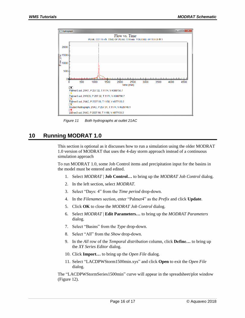
Both hydrographs will be plotted in a new window (Figure 11). Note the effects of the

detention basin on the incoming hydrograph. When selecting multiple hydrographs, view

all the selected hydrographs in a single plot by selecting Display | Open Hydrograph

Plot.

11. When done reviewing the Hydrograph dialog, close it by clicking the in the

top right corner.

12. Clear all the hydrograph results by selecting Hydrographs | Delete All.




Figure 11 Both hydrographs at outlet 21AC

10 Running MODRAT 1.0

This section is optional as it discusses how to run a simulation using the older MODRAT

1.0 version of MODRAT that uses the 4-day storm approach instead of a continuous

simulation approach

To run MODRAT 1.0, some Job Control items and precipitation input for the basins in

the model must be entered and edited.


2. In the left section, select MODRAT.

3. Select “Days: 4” from the Time period drop-down.




dialog.

7. Select “Basins” from the Type drop-down.


9. In the All row of the Temporal distribution column, click Define… to bring up

the XY Series Editor dialog.

10. Click Import… to bring up the Open File dialog.

11. Select “LACDPWStorm1500min.xys” and click Open to exit the Open File

dialog.

The “LACDPWStormSeries1500min” curve will appear in the spreadsheet/plot window

(Figure 12).



Figure 12 LACDPWStormSeries1500min curve plot

12. Click OK to close the XY Series Editor dialog and assign this curve to all basins.

Note that the rainfall depths entered do not need to be changed due to running a 4th day

simulation with MODRAT 2.0. These depths correspond to a 24 hour design storm and

are appropriate with the 1500 min. curve used with MODRAT 1.0.

13. Click OK to close the MODRAT Parameters dialog.


dialog.




17. Turn on Save file before run and click OK to close the MODRAT Run Options

dialog and bring up the Model Wrapper dialog.

18. Once MODRAT 1.0 finishes, turn on Read solution on exit and click Close to

exit the Model Wrapper dialog and import the solutions.


to each basin and outlet. Feel free to review the hydrographs as desired.

11 Conclusion

This concludes the “MODRAT Schematic” tutorial. Key concepts discussed and

demonstrated include some of the options available for using the MODRAT model in

WMS. Feel free to continue experimenting with the different options to become familiar

with all the capabilities in WMS for doing MODRAT simulations.

wms tutorials modrat schematic v. 11wmstutorials-11.0.aquaveo.com/modratschematic.pdf · wms saves...

Documents