WMS Investigation: Travel Time Variability with

Method, Area, and Slope

Ryan Murdock

May 1, 2001

Data Collection

• USGS DEMs – 30m resolution– UTM projection– 3 locations

• Cuyahoga River: Cleveland, Ohio

• Provo River: Provo, Utah

• Town Creek: Johnson City, Texas

• DRG background maps

Watershed Delineation

• Smooth DEM

• Flow directions & flow accumulations

• Convert raster streams to feature arcs

• Choose outlet

• Set accumulation threshold

• Delineate basin boundaries

• Convert basin to polygon

• Compute basin data

Choosing Accumulation Threshold

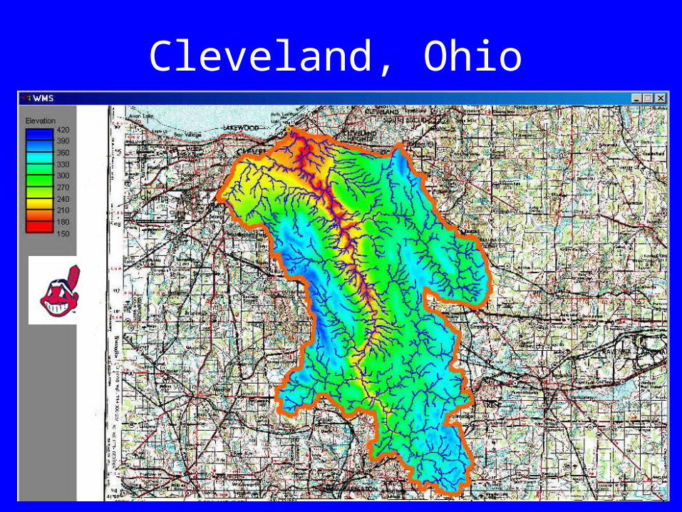
Cleveland, Ohio

Johnson City, Texas

South Fork of Provo River, Utah

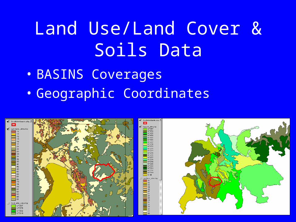
Land Use/Land Cover & Soils Data

• BASINS Coverages

• Geographic Coordinates

Projecting and Clipping• ArcView

– Project land use and soils data to UTM Zone 12 using the Projector Utility

– Export basin boundary from WMS– Clip themes using Spatial Analyst

Geoprocessing Wizard

Coverages in WMS

• Import shapefiles into WMS

• Assign land use and soil type coverages

Automated CN Calculation

• Import CN table

• Composite CN=0.5?

• Estimated CN=75

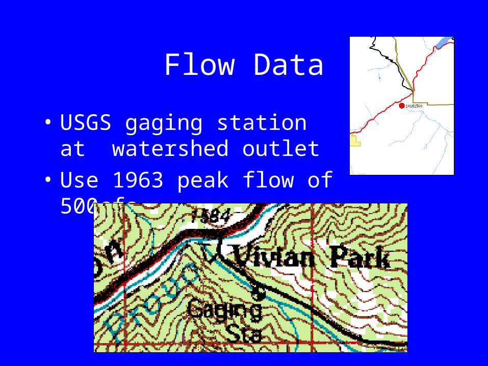
Flow Data

• USGS gaging station at watershed outlet

• Use 1963 peak flow of 500cfs

HEC-1

• Calibrate to measured peak flow by changing precipitation

• Basin average precipitation, type II-24 hr series

• SCS curve number method

• SCS unit hydrograph

Hydrographs!

• P=1.22 in, CN=65

Travel Time Calculator

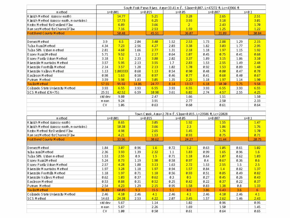
methodKirpich Method (grassy earth) 14.77 5.21 3.28 2.65 2.51Kirpich Method (grassy earth, mountains) 17.73 6.25 3.93 3.18 3.01Kerby Method for Overland Flow 6.89 3.66 2 2.43 1.70Ramser Method for Channel Flow 7.16 2.53 1.59 1.25 1.22Fort Bend County Method 50.48 45.51 36.07 31.89 30.84

Denver Method 3.9 6.5 2.04 3.40 1.52 2.53 1.73 2.88 1.29 2.15Tulsa Rural Method 4.34 7.23 2.56 4.27 2.03 3.38 1.82 3.03 1.77 2.95Tulsa 50% Urban method 2.81 4.68 1.66 2.77 1.31 2.18 1.18 1.97 1.15 1.92Espey Rural Method 5.71 9.52 1.3 2.17 0.64 1.07 0.45 0.75 0.41 0.68Espey Partly Urban Method 3.18 5.3 2.33 3.88 2.02 3.37 1.89 3.15 1.86 3.10Riverside Mountains Method 3.57 5.95 2.13 3.55 1.7 2.83 1.53 2.55 1.49 2.48Riverside Foothills Method 2.14 3.57 1.28 2.13 1.02 1.70 0.92 1.53 0.89 1.48Riverside Valleys Method 1.13 1.883333 0.68 1.13 0.54 0.90 0.48 0.80 0.47 0.78Eagleson Method 0.98 1.63 0.58 0.97 0.46 0.77 0.41 0.68 0.40 0.67Putnam Method 3.59 5.98 1.83 3.05 1.35 2.25 1.18 1.97 1.14 1.90Taylor Method 57.55 95.92 14.86 24.77 8.14 13.57 6.18 10.30 5.75 9.58Colorado State University Method 3.93 6.55 3.93 6.55 3.93 6.55 3.93 6.55 3.93 6.55SCS Method (CN=75) 25.51 42.52 6.59 10.98 3.61 6.02 2.74 4.57 2.55 4.25

std dev 9.80 2.47 1.66 1.51 1.50mean 9.24 3.91 2.77 2.50 2.33CV 1.06 0.63 0.60 0.61 0.64

methodKirpich Method (grassy earth) 8.65 3.05 1.92 1.55 1.47Kirpich Method (grassy earth, mountains) 10.38 3.66 2.3 1.86 1.76Kerby Method for Overland Flow 4.98 2.65 1.45 1.76 1.70Ramser Method for Channel Flow 4.21 1.53 0.93 0.75 0.71Fort Bend County Method 33.96 30.62 24.27 21.44 20.75

Denver Method 1.84 3.07 0.96 1.6 0.72 1.2 0.63 1.05 0.61 1.02tulsa rural Method 2.36 3.93 1.39 2.32 1.1 1.83 0.99 1.65 0.96 1.6Tulsa 50% Urban method 1.53 2.55 0.9 1.5 0.71 1.18 0.64 1.07 0.62 1.03Espey Rural Method 5.24 8.73 1.19 1.98 0.58 0.97 0.4 0.67 0.36 0.6Espey Partly Urban Method 2.57 4.28 1.88 3.13 1.63 2.72 1.53 2.55 1.5 2.5Riverside Mountains Method 1.97 3.28 1.18 1.97 0.94 1.57 0.84 1.4 0.82 1.37Riverside Foothills Method 1.18 1.97 0.71 1.18 0.56 0.93 0.51 0.85 0.49 0.82Riverside Valleys Method 0.62 1.03 0.37 0.62 0.3 0.5 0.27 0.45 0.26 0.43Eagleson Method 0.53 0.88 0.31 0.52 0.25 0.42 0.22 0.37 0.22 0.37Putnam Method 2.54 4.23 1.29 2.15 0.95 1.58 0.83 1.38 0.8 1.33Taylor Method 36.03 60.05 9.3 15.5 5.1 8.5 3.86 6.43 3.6 6Colorado State University Method 2.46 4.10 2.46 4.1 2.46 4.1 2.46 4.10 2.46 4.1SCS Method 14.63 24.38 2.53 4.22 2.07 3.45 1.57 2.62 1.46 2.43

std dev 5.67 1.14 1.02 0.96 0.95mean 5.67 2.26 1.69 1.50 1.45CV 1.00 0.50 0.61 0.64 0.65

s=0.05s=0.015South Fork Provo River, Area=33.41 mi2, Slope=0.087, L=47272 ft, Lc=43966 ft

Town Creek, Area=2.78 mi2, Slope=0.015, L=23586 ft, Lc=22028s=0.001 s=0.015 s=0.05 s=0.087 s=0.1

s=0.001 s=0.1s=0.087

Assumptions/Simplifications

• Each basin– Same % impervious– Same CN– Same roughness– Changed slopes in calculator, not re-delineated

Analysis

• More dispersion of results in larger basins

• Increasing slope causes the standard deviations to decrease

• No strong trends with slope in the coefficient of variation

• Different sized basins with the same slope have similar coefficients of variation

Equation Evaluation

• Pretty Robust– Putnam, Kerby, Denver

• Touchy– Fort Bend County– Taylor

• SCS method predicts longer travel time• Remember the conditions under which the

equations were developed

Time is Running Out…

• Revisit the composite CN process– Confidence in HEC-1 calibration

• Include Cuyahoga River travel time results

• Look at the equivalent velocities represented by each equation/method

That's the end of today’s modeling adventures, kids.