wms 9.0 tutorial watershed modeling modrat interface (gis ...wmstutorials-9.0.aquaveo.com/17...

of 21 © Aquaveo 2012

WMS 9.0 Tutorial

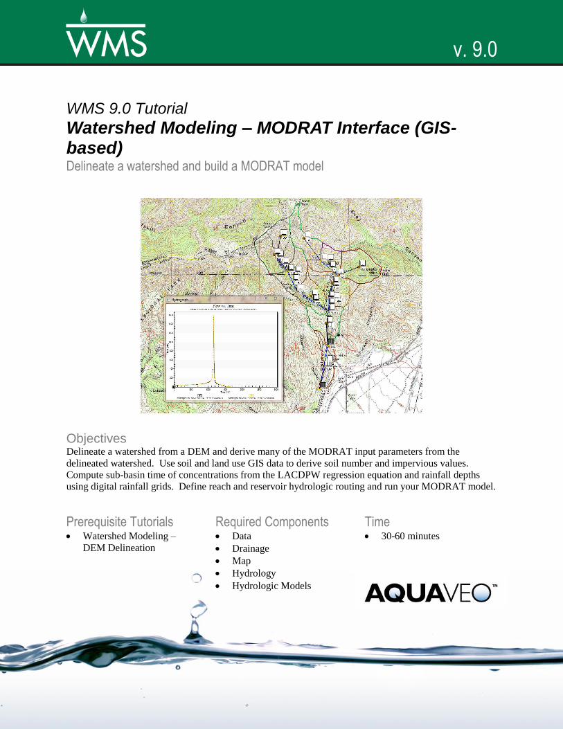
Watershed Modeling – MODRAT Interface (GIS-based) Delineate a watershed and build a MODRAT model

Objectives Delineate a watershed from a DEM and derive many of the MODRAT input parameters from the

delineated watershed. Use soil and land use GIS data to derive soil number and impervious values.

Compute sub-basin time of concentrations from the LACDPW regression equation and rainfall depths

using digital rainfall grids. Define reach and reservoir hydrologic routing and run your MODRAT model.

Prerequisite Tutorials Watershed Modeling –

DEM Delineation

Required Components Data

Drainage

Map

Hydrology

Hydrologic Models

Time 30-60 minutes

v. 9.0


1 Contents

1 Contents ............................................................................................................................... 2 2 Introduction ......................................................................................................................... 2 3 Objectives ............................................................................................................................. 2 4 Delineating the Watershed ................................................................................................. 3

4.1 Delineate the Watershed ............................................................................................... 4 5 MODRAT Global Setup ..................................................................................................... 8

5.1 Job Control ................................................................................................................... 8 5.2 Tree Numbering ........................................................................................................... 8

6 MODRAT Basin Data Setup .............................................................................................. 9 6.1 Basin Data Parameters ............................................................................................... 10 6.2 Soil Number Computation ......................................................................................... 10 6.3 Percent Impervious Computation ............................................................................... 11 6.4 Rainfall Depth and Distribution Assignment ............................................................. 12 6.5 Time of Concentration ............................................................................................... 13

7 MODRAT Reach/Outlet Data Setup ............................................................................... 14 8 Running a MODRAT 2.0 Simulation .............................................................................. 15 9 Burned Watershed Simulation ......................................................................................... 16 10 Debris Production ............................................................................................................. 18

10.1 DPA Zones ................................................................................................................. 18 10.2 Debris Control Structures ........................................................................................... 19 10.3 Reports ....................................................................................................................... 20

11 Bulking Flows .................................................................................................................... 20 12 Conclusion.......................................................................................................................... 21

2 Introduction

WMS has a graphical interface to the Los Angeles County Dept. of Public Works

(LACDPW) Modified Rational (MODRAT) model. Geometric attributes such as areas,

lengths, and slopes are computed automatically from the digital watershed. Parameters

such as soil numbers, impervious percentages, and routing data are entered through a

series of interactive dialog boxes. Once the parameters needed to define an MODRAT

model have been entered, an input file with the proper format for MODRAT can be

written automatically. Since only parts of the MODRAT input file are defined in this

exercise, you are encouraged to explore the different available options of each dialog,

being sure to select the given method and values before exiting the dialog.

3 Objectives

As a review you will delineate a watershed from a DEM. You will then develop a simple

watershed model using the delineated watershed to derive many of the parameters. Land

use and soil shape files will be used to develop a soil number and impervious values.

Time of concentration will be computed using the LACDPW regression equation.

Rainfall depths will be computed from digital rainfall grids for Los Angeles County.

After establishing the initial MODRAT model other variations will be developed,

including defining reach routing and including a reservoir with storage routing.

WMS Tutorials Watershed Modeling – MODRAT Interface (GIS-based)


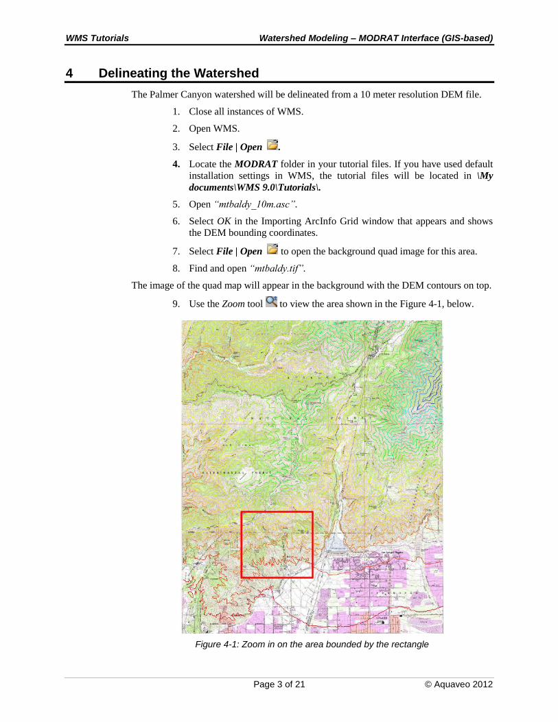
4 Delineating the Watershed

The Palmer Canyon watershed will be delineated from a 10 meter resolution DEM file.

1. Close all instances of WMS.

2. Open WMS.

3. Select File | Open .

4. Locate the MODRAT folder in your tutorial files. If you have used default

installation settings in WMS, the tutorial files will be located in \My

documents\WMS 9.0\Tutorials\.

5. Open “mtbaldy_10m.asc”.

6. Select OK in the Importing ArcInfo Grid window that appears and shows

the DEM bounding coordinates.

7. Select File | Open to open the background quad image for this area.

8. Find and open “mtbaldy.tif”.

The image of the quad map will appear in the background with the DEM contours on top.

9. Use the Zoom tool to view the area shown in the Figure 4-1, below.

Figure 4-1: Zoom in on the area bounded by the rectangle



4.1 Delineate the Watershed

1. Switch to the Drainage module .

2. Select DEM | Compute Flow Direction/Accumulation....

3. Select OK.

4. Select the Current Projection button in the Units dialog.

5. Select the Global Projection button in the Current Projection dialog.

6. Set the Projection to State Plane Coordinate System.

7. Set Zone to California Zone 5 (FIPS 405).

8. Set the Datum to NAD83.

9. Set Planar Units to Feet (U.S. Survey).

10. Select OK on the Select Projection dialog.

11. Set the Vertical Projection to NGVD 29 (US) and Units to U.S. Survey

Feet.

12. Select OK – you have now told WMS what the units and projections are for

the raw DEM data you have loaded and are about to process.

13. Set the Basin Areas to Acres; leave the Distances in Feet. WMS will report

computed geometric parameters in these units after you delineate the

watershed.

14. Select OK in the Units dialog to begin the TOPAZ processing.

15. Select Close once TOPAZ finishes running (you may have to wait for the

computer to finish processing the information).

Blue lines will appear on the DEM indicating location of flow accumulation channels

(streams). You will need to edit the display to match the channel complexity desired.

16. Select Display | Display Options .

17. Choose DEM Data and set Point Display Step to 1 and Min. Accumulation

for Display to 40.0.

18. Select OK – note the change in the flow accumulation stream network.

You are now ready to define the main watershed outlet location and define the drainage

area. You will then define interior outlet points and let WMS subdivide the watershed.

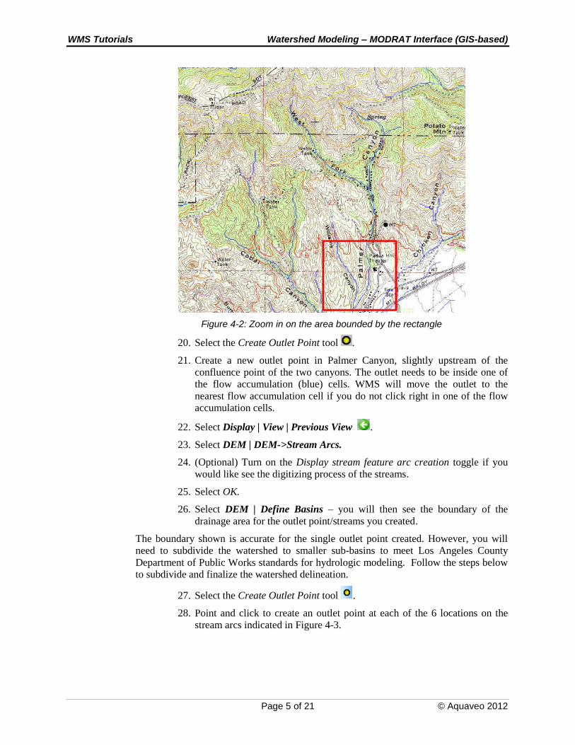
19. Use the Zoom tool to view the area shown in Figure 4-2 which shows

the confluence of Palmer Canyon and Williams Canyon.



Figure 4-2: Zoom in on the area bounded by the rectangle

20. Select the Create Outlet Point tool .

21. Create a new outlet point in Palmer Canyon, slightly upstream of the

confluence point of the two canyons. The outlet needs to be inside one of

the flow accumulation (blue) cells. WMS will move the outlet to the

nearest flow accumulation cell if you do not click right in one of the flow

accumulation cells.

22. Select Display | View | Previous View .

23. Select DEM | DEM->Stream Arcs.

24. (Optional) Turn on the Display stream feature arc creation toggle if you

would like see the digitizing process of the streams.

25. Select OK.

26. Select DEM | Define Basins – you will then see the boundary of the

drainage area for the outlet point/streams you created.

The boundary shown is accurate for the single outlet point created. However, you will

need to subdivide the watershed to smaller sub-basins to meet Los Angeles County

Department of Public Works standards for hydrologic modeling. Follow the steps below

to subdivide and finalize the watershed delineation.

27. Select the Create Outlet Point tool .

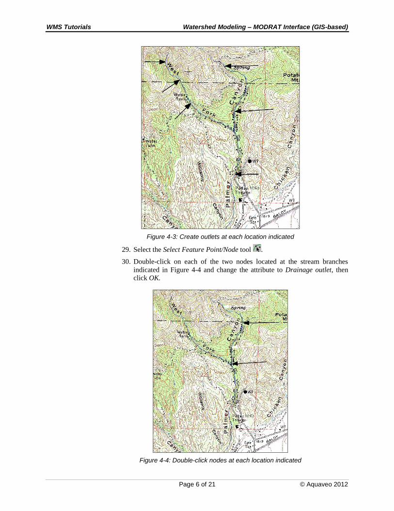
28. Point and click to create an outlet point at each of the 6 locations on the

stream arcs indicated in Figure 4-3.



Figure 4-3: Create outlets at each location indicated

29. Select the Select Feature Point/Node tool .

30. Double-click on each of the two nodes located at the stream branches

indicated in Figure 4-4 and change the attribute to Drainage outlet, then

click OK.

Figure 4-4: Double-click nodes at each location indicated



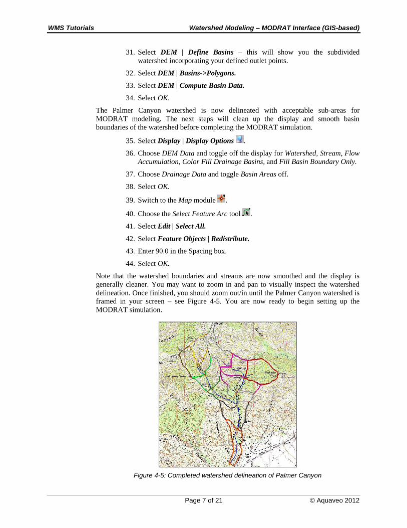
31. Select DEM | Define Basins – this will show you the subdivided

watershed incorporating your defined outlet points.

32. Select DEM | Basins->Polygons.

33. Select DEM | Compute Basin Data.

34. Select OK.

The Palmer Canyon watershed is now delineated with acceptable sub-areas for

MODRAT modeling. The next steps will clean up the display and smooth basin

boundaries of the watershed before completing the MODRAT simulation.


36. Choose DEM Data and toggle off the display for Watershed, Stream, Flow

Accumulation, Color Fill Drainage Basins, and Fill Basin Boundary Only.

37. Choose Drainage Data and toggle Basin Areas off.

38. Select OK.

39. Switch to the Map module .

40. Choose the Select Feature Arc tool .

41. Select Edit | Select All.

42. Select Feature Objects | Redistribute.

43. Enter 90.0 in the Spacing box.

44. Select OK.

Note that the watershed boundaries and streams are now smoothed and the display is

generally cleaner. You may want to zoom in and pan to visually inspect the watershed

delineation. Once finished, you should zoom out/in until the Palmer Canyon watershed is

framed in your screen – see Figure 4-5. You are now ready to begin setting up the

MODRAT simulation.

Figure 4-5: Completed watershed delineation of Palmer Canyon



This is a good place to save your project to the hard drive before continuing. Save this

data to a WMS project file:

45. Select File | Save As .

46. Enter “PalmerCyn25_GIS.wms” and click Save.

47. Select No if asked to save image files in project directory.

WMS will save your project to a set of WMS Project files. The *.wms file is an index file

and contains other information that instructs WMS to load all the files associated with the

project when you open your project at a later time.

5 MODRAT Global Setup

The MODRAT analysis setup requires you to enter Job Control data, basin data for each

subarea, reach data for each channel, and elevation-storage-discharge relationships for

each storage facility. The following sections will guide you in entering data and using

GIS data layers to acquire input data for MODRAT.

5.1 Job Control

Most of the parameters required for a MODRAT model are defined for basins, outlets,

and reaches. However, there are a few “global” parameters that control the overall

simulation. These parameters are not specific to any basin or reach in the model. These

parameters are defined in the WMS interface using the Job Control dialog.

1. Switch to the Hydrologic Modeling module .

2. Select MODRAT from the drop down list of models found in the Models

Window – a MODRAT menu item will appear in the Menu Bar.

3. Select MODRAT | Job Control.

4. Choose MODRAT 2.0 at the top of the dialog.

5. Select 2 days in the Run time drop down list.

6. Select 25 year in the Storm Frequency drop down list.

7. Enter “palmergis1” in the Prefix box, then click Update. Note that the

default prefix for output files is now updated.

8. Enter “palmergis_rain.dat” in the Rain file box.

9. Click the browse button next to the Soil file and open the file

“sgr_soilx_71.dat”.

10. Select OK.

5.2 Tree Numbering

Each basin or reach is assigned a default name when it is created by WMS. However,

these must be named and numbered in sequential order from upstream to downstream

using a MODRAT naming convention so that MODRAT analyzes the model in the

proper order.



A-Lateral

1. Select the Select Basin tool .

2. Click on the brown square sub-basin icon at the most upstream end of

Palmer Canyon (the canyon forking to the right). Selecting this basin

defines the upstream end of

the main line of the

watershed.

3. Select MODRAT | Number

Tree.

4. Select OK to start numbering

with location/lateral of 1A.

5. As the numbering process

proceeds you will be

prompted to "Select a lateral"

for each of the basins at a

confluence. Notice that WMS

first zooms into a basin along

the "A" lateral and its surrounding outlet points. Since the outlet point

upstream from this basin is located on the "A" lateral (you can determine

this because the upstream outlet name ends with "A"), assign the first basin

to the "A" lateral of the watershed and select OK.

6. Now notice that WMS zooms

into a basin on the "B" lateral

and its surrounding outlet

points. Since the outlet point

upstream from this basin is

located on the "B" lateral (you

can determine this because the

upstream outlet name ends with

"B"), assign this basin to the

"B" lateral of the watershed and

select OK.

7. Right-click on the Drainage

coverage in the Project

Explorer and select Zoom To

Layer.

The numbering is now complete. Note that the selected basin is now 1A. The main line is

met by Line B at the 16AB confluence (outlet) point. The numbers now indicate the order

in which the units will be processed by MODRAT.

6 MODRAT Basin Data Setup

Each basin in the watershed requires a number of input parameters. Many of these can be

computed using tools in WMS.

B-Lateral



6.1 Basin Data Parameters

1. Double-click on the basin icon labeled 1A. You may need to toggle the

mtbaldy image off in the Project Explorer to better see the basin labels.

Double-clicking on a basin or outlet icon brings up the parameter editor dialog for the

current model (in this case MODRAT)

2. Notice that the area has been calculated but all other parameters are empty.

3. Click OK to exit the window.

Many of the parameters can be computed by WMS using GIS data layers. The following

sections will compute Soil Number, Percent Impervious, and Rainfall Depth for each

basin.

6.2 Soil Number Computation

You will load soil data for Los Angeles County and let WMS compute the dominant soil

type for each basin.

1. Right-click on the Coverages folder in the Map Data section of the Project

Explorer.

2. Choose New Coverage from the pop-up menu.

3. Select Soil Type as the Coverage Type in the

Properties window.

4. Select OK.

5. Switch to the GIS module .

6. Select Data | Add Shapefile Data.

7. Open “soils_2004.shp” from the

MODRAT\SoilType folder – the soil map for all

of L.A. County will be loaded.

8. Right-click on the Drainage coverage in the Project Explorer and select

Zoom To Layer.

9. Select the Soil Type coverage.

10. Switch back to the GIS module .

11. Choose the Select Shapes tool .

12. Drag a selection box around the watershed extents – the soil polygons

covering the watershed will be selected.

13. Select Mapping | Shapes -> Feature Objects.

14. Select Next.

15. Make sure the CLASS field is mapped to the LA County soil type attribute.

16. Select Next.

17. Select Finish.



18. Hide the soils_2004.shp file by deselecting its check box in the Project

Explorer.

Now that the soil data is loaded, do the following to compute and assign the soil numbers

to MODRAT:

19. Select the Drainage coverage in the Project Explorer to designate it as the

active coverage.

20. Select the Hydrologic Modeling module .

21. Select MODRAT | Map Attributes.

22. Select LA County soil numbers as the Computation type.

23. Select OK.

24. Once the computation is finished, double-click on any sub-basin icon to

bring up the MODRAT Parameters window and view the Soil number

assigned.

25. Click OK to exit the MODRAT Parameters window.

6.3 Percent Impervious Computation

You will now load land use data for Los Angeles County and let WMS compute the

average percent impervious for each basin.


Explorer.

2. Choose New Coverage in the pop-up menu.

3. Select Land Use as the Coverage Type in the Properties window.

4. Select OK.



7. Open “landuse_imp_2004.shp” in the MODRAT\Landuse folder – the

land use map for all of L.A. County will be loaded.


Zoom To Layer.

9. Select the Land Use coverage.



12. Drag a selection box around the watershed extents – the land use polygons

covering the watershed will be selected.


14. Select Next.

15. Make sure the IMPERV_ field is mapped to the Percent Impervious

attribute.



16. Select Next.

17. Select Finish.

18. Hide the landuse_imp_2004.shp file by toggling off its check box in the

Project Explorer.

Now that the land use data is loaded, do the following to compute and assign the percent

impervious to MODRAT.

19. Select the Drainage coverage in the Project Explorer to designate it as the

active coverage.


21. Select MODRAT | Map Attributes.

22. Select LA County land use as the Computation type.

23. Select OK.


bring up the MODRAT Parameters window and view the Impervious %

assigned.


6.4 Rainfall Depth and Distribution Assignment

You will now load a rainfall depth grid for the 25-year storm frequency for Los Angeles

County and let WMS compute the average rainfall depth for each sub-basin. Then you

will assign a rainfall mass curve to the model to provide the temporal distribution of the

storm depth.

1. Select the Drainage module .

2. Select File | Open .

3. Change the File Type to Rainfall Depth Grid (*.*).

4. Open the file named “lac25yr24hr.asc” in the MODRAT folder – the

rainfall grid will be opened and displayed.


Zoom To Layer.


7. Select Calculators | Compute GIS Attributes.

8. Select Rainfall Depth as the Computation.

9. Select OK.

10. Choose the Select Basin tool and double-click on basin 1A to bring up

the MODRAT Parameters window and view the rainfall depth assigned.

11. Choose Show: All in the upper left part of the dialog.

12. In the Temporal distribution column click on the Define… button in the All

row (colored yellow) of the spreadsheet. This will bring up a window



where you will specify the rainfall temporal distribution (time vs.

cumulative rainfall percentage).

13. Select the Import button in the XY Series Editor.

14. Open the file named “LACDPWStorm-4thday.xys”.

15. The Selected Curve in the XY Series Editor should now read

LACDPWStorm-4thday and the rainfall mass curve is displayed.

16. Select OK.

17. Select OK.

The process above has assigned a rainfall depth to each basin and also assigned the

LACDPW storm distribution curve to all basins.

Clean up the display of your model by turning off several layers now that they have been

used and are not needed:

18. Hide the Soil Type coverage by toggling off its check box in the Project

Explorer.

19. Hide the Land Use coverage by toggling off its check box in the Project

Explorer.

20. Hide the Rain Fall grid file by toggling off its check box in the Project

Explorer.

21. Hide the mtbaldy image by toggling off its check box in the Project

Explorer.

6.5 Time of Concentration

The final parameter needed for each basin in the model is the Time of Concentration

(Tc). WMS has the LACDPW Tc equation method built in and linked to GIS data

capabilities. Do the following to compute Tc for all basins.

1. Select the Drainage module .

2. Select DEM | Compute Basin Data.

3. In the Units dialog, select the Drain Data Compute Opts... button. Toggle

on the checkbox to Create Tc Coverage.

4. Select OK, and then OK again on the Units dialog.

Note the basin data is recomputed (basin area is displayed) and there is a new coverage

named Time Computation and containing the longest flow path of each basin.


6. Choose Drainage Data and toggle Basin Areas off.

7. Select OK.

8. Ensure that the Drainage coverage is the active coverage by selecting it in

the Project Explorer.


10. Select MODRAT | Compute Tc.



11. Note that a check of required input for Tc computations has been

performed. Select Next in the Compute MODRAT Tc Wizard.

12. Review the Time of Concentration (Tc) computed for each basin.

13. Select Done.


bring up the MODRAT Parameters window and view the Tc assigned.


The input parameters for all basins should now be entered for the simulation. Save this

data to your working project file.

16. Select File | Save .

17. Select No if asked to save image files in the project directory.

7 MODRAT Reach/Outlet Data Setup

Each reach must have data associated with it to be successfully simulated by MODRAT.

Reaches are selected in WMS by clicking on an outlet (confluence) point. The parameters

for that point, and the channel downstream from that point to the next, can be edited.

1. Double-click the outlet labeled 2A at the upper end of the Palmer Canyon

main channel – this will load the parameters for that reach into the

MODRAT Parameters window for review/editing.

Note that Length and Slope have been computed and are entered in the MODRAT

Parameters window.

2. Select Mountain as the Routing Type.

Note that the Manning’s n box is inactive and no additional variables need to be entered

for this channel type.

3. Choose Hydrograph (*.HYF) and WMS plot file (*.SOL) for the

Hydrograph Output.

You have now completed the input for one of the reaches in the Palmer Canyon

watershed. You will need to define data for all reaches in a similar fashion:

4. Choose Show: All from the drop-down box in the upper-right corner.

5. Use the table below to fill in values:

Reach Name Routing type n Output

2A Mountain - HYF/SOL

5A Valley - HYF/SOL

7A Valley - HYF/SOL

10B Mountain - HYF/SOL

12B Mountain - HYF/SOL

14B Valley - HYF/SOL

16AB Valley - HYF/SOL

18A Valley - HYF/SOL

20A Variable 0.014 HYF/SOL



6. Note that Reach 20A, the most downstream outlet, does not need a length

or slope defined since it is at the downstream end of the watershed. When

you are finished entering the parameters choose OK on the MODRAT

Parameters dialog.

The input parameters for all reaches should now be entered for the simulation. Save this

data to your working project file.

7. Select File | Save .

8. Select No if asked to save image files to the project directory.

8 Running a MODRAT 2.0 Simulation

All the data required to run a simulation is now ready. To make sure there are no

omissions in the data, WMS will perform a model check. Follow the steps below:

1. Select MODRAT | Check Simulation

2. Review the model check report noting that there are 2 possible errors in the

MODRAT model.

Notice the line stating “No reach length is defined for outlet 20A”. The outlet 20A is the

watershed outlet; therefore, there is no reach downstream that you need to define.

3. Select Done to exit the MODRAT Model Check.

The model checker is a simple way to verify that you have not left out any needed data. It

does not verify that the model is correct, but that all the data needed to run the simulation

is in place. To execute the MODRAT simulation, do the following:

4. Select MODRAT | Run Simulation.

5. The Input File should be named “Palmergis1.lac”.

6. Ensure that the Save file before run toggle is checked.

7. Ensure that the Prefix for output files box contains “Palmergis1”.

8. Click OK to start the simulation.

A window will appear and report the progress of the MODRAT simulation.

9. Select Close once MODRAT finishes running (you may have to wait a few

seconds to a minute or so).

The resulting hydrographs will be read in and a small hydrograph plot will appear next to

each basin and outlet.

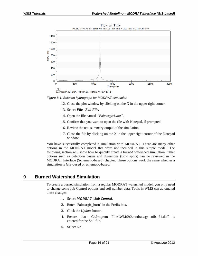
10. Double-click on the hydrograph icon next to outlet 20A.

11. Review the hydrograph plot that appears in a new plot window. It should

look similar to Figure 8-1.



Figure 8-1: Solution hydrograph for MODRAT simulation

12. Close the plot window by clicking on the X in the upper right corner.

13. Select File | Edit File.

14. Open the file named “Palmergis1.out”.

15. Confirm that you want to open the file with Notepad, if prompted.

16. Review the text summary output of the simulation.

17. Close the file by clicking on the X in the upper right corner of the Notepad

window.

You have successfully completed a simulation with MODRAT. There are many other

options in the MODRAT model that were not included in this simple model. The

following section will show how to quickly create a burned watershed simulation. Other

options such as detention basins and diversions (flow splits) can be reviewed in the

MODRAT Interface (Schematic-based) chapter. Those options work the same whether a

simulation is GIS-based or schematic-based.

9 Burned Watershed Simulation

To create a burned simulation from a regular MODRAT watershed model, you only need

to change some Job Control options and soil number data. Tools in WMS can automated

these changes:

1. Select MODRAT | Job Control.

2. Enter “Palmergis_burn” in the Prefix box.

3. Click the Update button.

4. Ensure that “C:\Program Files\WMS90\modrat\sgr_soilx_71.dat” is

entered for the Soil file.

5. Select OK.



The Soil file designated in Job Control must contain soil data for burned conditions. The

sgr_soilx_71.dat file contains regular soil data for typical LA County soil numbers (2-

180) and for burned soil numbers (202-380). Now you will update all the soil numbers in

the watershed to reflect burned conditions.

6. Select MODRAT | Create Burned Simulation.

7. Ensure the default of 200 is entered for Burned soils increment – this is the

increment to be added to normal soils to get the corresponding burned soil.

8. Ensure that the impervious limit is set at 15% – basins with higher

impervious values will not be affected by the burn.

9. Select OK.


bring up the MODRAT Parameters window and view the new Soil type

number assigned.


12. Select MODRAT | Run Simulation.

13. The Input File should be named “Palmergis_burn.lac”.

14. Ensure that the Save file before run toggle is checked.

15. Ensure that the Prefix for output files box contains “Palmergis_burn”.

16. Click OK to start the simulation.

17. Select Close once MODRAT finishes running (you may have to wait a few

seconds to a minute or so).

The resulting hydrographs will be read in and a small hydrograph plot will appear next to

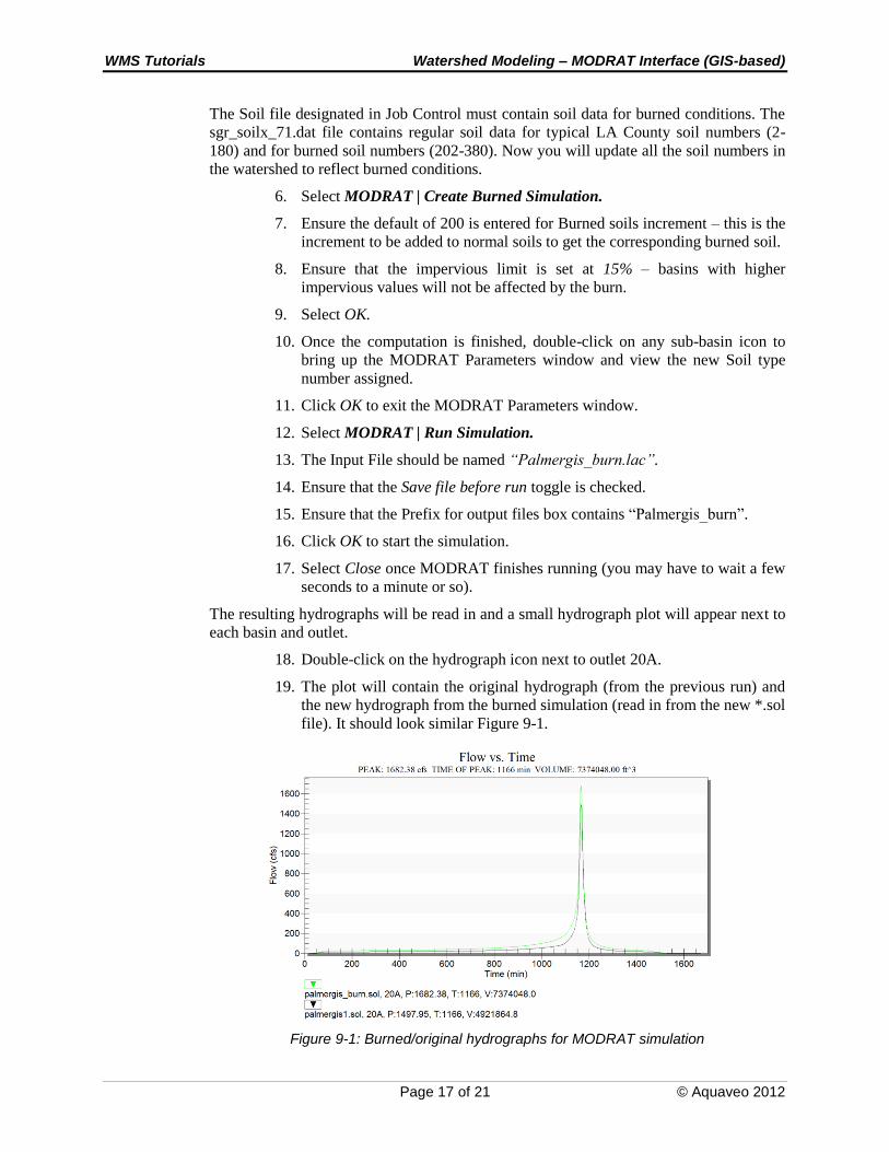
each basin and outlet.

18. Double-click on the hydrograph icon next to outlet 20A.

19. The plot will contain the original hydrograph (from the previous run) and

the new hydrograph from the burned simulation (read in from the new *.sol

file). It should look similar Figure 9-1.

Figure 9-1: Burned/original hydrographs for MODRAT simulation



20. Close the plot window by clicking on the X in the upper right corner.

21. Clear the results by selecting Hydrographs | Delete All.

10 Debris Production

WMS has a tool for computing the amount of debris produced as part of the runoff from

mountainous and burned drainage basins. The following sections demonstrate how to

compute debris production, account for debris control structures, and generate reports

detailing the calculations.

10.1 DPA Zones

The debris production calculator in WMS requires GIS data that defines debris

production area (DPA) zones. Drainage basin polygons are overlaid with the DPA zone

polygons in order to determine debris production rates, which are applied to the area

contributing to any outlet point of interest.


Explorer.

2. Choose New Coverage.

3. Select MODRAT DPA Zone as the Coverage Type in the Properties

window.

4. Select OK.



7. Open “dpazones.shp” – the Debris Production Area (DPA) zones for all of

L.A. County will be loaded.


Zoom To Layer.

9. Select the MODRAT DPA Zone coverage.



12. Drag a selection box around the watershed extents – the DPA zone

polygons covering the watershed will be selected.


14. Select Next.

15. Make sure the DPA_ZONES field is mapped to the DPA Zone attribute.

16. Select Next.

17. Select Finish.

18. Hide the dpazones.shp file by toggling off its check box in the Project

Explorer.



19. Switch to the Hydrologic Modeling module .

20. Select MODRAT|Debris Production\Bulking….

21. Click on the Compute GIS Data… button on the Basin data tab.

22. Verify that the MODRAT DPA Zone and Land Use coverages are selected

for this calculation.

23. Select OK.

24. Activate the Debris production tab in the dialog.

Total debris produced is reported for each outlet shown in the spreadsheet by summing

the debris produced within each DPA zone for all undeveloped drainage areas that

contribute runoff to the outlet.

10.2 Debris Control Structures

Adequate or undersized debris control structures can be defined at any outlet point and

included in debris production calculations for all downstream outlets.

1. In the 5A column of the spreadsheet click on the Control structures View…

button.

All of the outlets located upstream of outlet 5A are listed in this dialog.

2. Toggle on the checkbox next to location 2A.

3. Ensure that the Size is set to Adequate.

4. Select OK.

Notice that the debris calculations are automatically updated. An adequately sized

control structure will remove all debris produced upstream of the location of the control

structure from the results reported at all downstream locations.

5. In the 5A column of the spreadsheet click on the Control structures View…

button.

6. Change the Size to Undersized.

7. Enter 10,000.00 for Capacity.

8. Set the Units to yd^3.

9. Select OK.

Values now show up in the Excess controlled debris row of the spreadsheet and are

included in the total debris reported for all outlets downstream of the control structure.

10. In the 5A column of the spreadsheet click on the View… Control structures

button.

11. Set the Units to (%).

12. Enter 0.5 for Capacity (only decimal percentages are valid).

13. Select OK.

In this case 50% of the debris produced upstream of the control structure is contained and

the other 50% of the debris in included in the total debris reported for all outlets

downstream of the control structure.



10.3 Reports

It is important to understand the difference between using report nodes and exporting a

report that details the debris production computations.

1. Click on the All On button.

This marks all of the outlets displayed in the spreadsheet as report nodes. Report node

locations are saved with the WMS project file and are used to indicate which outlets are

of interest within a specific project. For example:

2. Click on the All Off button.

3. Toggle on the checkbox for outlet 5A in the spreadsheet to mark it as a

report node.

4. Set the Show option to Report nodes (upper left corner of dialog).

Now only the data for outlet 5A is shown in the spreadsheet. There is also an option for

showing outlets selected in the graphics window.

5. Click on the Export… button.

6. Click Save to save the report using the default location and file name.

7. Click OK in the Debris Production dialog.

8. Select File | Edit File…

9. Open “ladebris.txt”.

Reports will include both summary and detailed data for all outlets that appear in the

spreadsheet when exported. In this case only data for outlet 5A is included in the report

because that was the only data shown in the spreadsheet at the time that the report was

exported.

10. Close the file by clicking on the X in the upper right corner of the Notepad

window.

11 Bulking Flows

Burned flow rates are bulked in order to account for the debris/sediment in the runoff

flow rate. Bulking factors are determined using DPA zones. The Bulked Flow calculator

operates in the same fashion as the Debris Production calculator, including accounting for

the effects of debris control structures. Burned flow values can be directly entered into

the spreadsheet or read from a MODRAT solution.

1. Select MODRAT | Debris Production/Bulking….

2. Activate the Bulked flow tab.

3. Click on the Get Burned Flows From MODRAT Solution… button.

4. Open “Palmergis_burn.out”.

The bulked flow values in the spreadsheet are automatically updated. Click on the

Control structures View… button in column 5A of the spreadsheet to experiment with

combining debris control structures with flow bulking.



12 Conclusion

This concludes the exercise on defining MODRAT files and displaying hydrographs. The

concepts learned include the following:

Entering job control parameters

Defining basin parameters from GIS data

Defining routing parameters

Saving MODRAT input files

Reading hydrograph results

Creating a burned simulation

Debris production and flow bulking

Comparing results from two runs

There are many other options in the MODRAT that were not included in this simple

model. Other options such as detention basins and diversions (flow splits) can be

reviewed in the MODRAT Interface (Schematic-based) chapter. Those options work the

same whether a simulation is GIS-based or schematic-based.

wms 9.0 tutorial watershed modeling modrat interface (gis ...wmstutorials-9.0.aquaveo.com/17...

Documents