wireless sensor networks for monitoring cracks in … university wireless sensor networks for...
TRANSCRIPT

NORTHWESTERN UNIVERSITY
Wireless Sensor Networks for Monitoring Cracks in Structures
A THESIS
SUBMITTED TO THE GRADUATE SCHOOL
IN PARTIAL FULFILLMENT OF THE REQUIREMENTS
for the degree
Master of Science
Field of Civil Engineering
By
Mathew P. Kotowsky
EVANSTON, ILLINOIS
June 2010


i
ABSTRACT
Autonomous Crack Monitoring (ACM) and Autonomous Crack Propagation Sensing (ACPS)
are two types of structural health monitoring in which characteristics of cracks are recorded over
long periods of time. ACM seeks to correlate changes in widths of cosmetic cracks in structures
to nearby blasting or construction vibration activity for the purposes of litigation or regulation.
ACPS seeks to track growth of cracks in steel bridges, supplementing regular inspections and
alerting stakeholders if a crack has grown.
Both ACM and ACPS may be implemented using wired data loggers and sensors, however,
the cost of installation and intrusion upon the use of a structure makes the use of these sys-
tems impractical if not completely impossible. This thesis presents the implementation of these
systems using wireless sensor networks (WSNs) and evaluates the effectiveness of each.
Three wireless ACM test deployments are presented: the first a proof of concept, the second
to show long-term functionality, and the third to show the effectiveness of a newly invented
device for low-power event detection. Each of these case studies was performed in a residential
structure.
Four laboratory experiments of ACPS systems and sensors are presented: the first three
show the functionality of commercially available crack propagation sensors and a WSN sys-
tem adapted from the agricultural industry. The final experiment shows the functionality of a
newly invented form of crack propagation gage that allows for a more flexible installation of
the sensor.


iii
Acknowledgements
This thesis represents the climax of a serendipitous chapter in my career in which I found anunexpected outlet in civil engineering for my interest and skills in computers and electronics.Many teachers, co-workers, family and friends have been a part of this process, and to them Igive my most sincere thanks.
First, I would like to thank my M.S. thesis committee, Professor Charles H. Dowding andProfessor David J. Corr for their guidance and direction during my entire graduate school ex-perience. Entering the field of civil engineering with an undergraduate background in computerengineering was a challenge through which these two gentlemen saw me with advice on every-thing from course selection to conference attendance and everything in between.
While I was a sophomore in computer engineering at the University of Illinois at Urbana-Champaign, Professor Dowding hired me as an undergraduate programmer to assist over the In-ternet and on school breaks in his Autonomous Crack Monitoring project sponsored by North-western University’s Infrastructure Technology Institute (ITI). This unusual employment ar-rangement blossomed into a summer internship at ITI, employment after graduation, and even-tually entrance into graduate school. Instead of moving to California to write software for alarge company in Silicon Valley, I have spent the last several years of my life travelling thecountry and applying my computer and civil engineering education to exciting instrumentationprojects.
Professor Corr only recently joined the ITI team, but his industry experience and expertisein structural engineering immediately strengthened my work at ITI and gave me a fresh per-spective on all of my efforts. Both in the classroom and in the field, Professor Corr reinforcedmy understanding of structural engineering concepts that were newer to me than to my class-mates and gave me the confidence to go forward with my experiments in custom-designed crackpropagation sensors.
The late Professor David F. Schulz, founding director of ITI, brought together a team ofengineers that have turned my college job into a viable career path. Professor Schulz, andcurrent ITI Director Joseph L. Schofer, have made available to me a world of engineering ex-periences that I could not have imagined as an undergraduate. To these gentlemen I am deeply

iv
indebted. Nearly all of the research described in this thesis was funded by ITI via its grantfrom the Research and Innovative Technology Administration of the United States Departmentof Transportation.
The ITI Research Engineering Group, Daniel R. Marron, David E. Kosnik, and the lateDaniel J. Hogan, have been my closest partners during my time at Northwestern. From thesethree gentlemen I have learned more than from any classroom teacher. We have travelled thecountry together from the Everglades to the Pacific Northwest, at every destination encounteringunique challenges and meeting them as a team. From Mr. Hogan, I learned that befriending aman with a welder can solve more problems than you might think, especially when you needto drop the anchor. From Mr. Marron I learned that any engineering task is possible if you’renear enough to a hardware store. From Mr. Kosnik I learned that I can be as fascinated bya coincidental juxtaposition of municipal and private water towers as by staring upward frominside the construction site at the World Trade Center. These and other life lessons learnedwhile part of the Research Engineering Group will stay with me for the rest of my engineeringcareer.
Without the contributions of undergraduate research assistant Ken Fuller, the experimentsin Chapter 4 would have been impossible. Mr. Fuller assisted me by completing almost all ofthe preparation of the test coupons, accompanying me to the industrial paint warehouse, andmaking himself available for long hours in the mechanical testing lab. His reliability, workethic, attention to detail, and camaraderie were invaluable to me.
Melissa Mattenson, an old friend and more recently my next-door neighbor at the office,contributed vastly to my graduate work with a steady stream of gummy stars, needless (or werethey?) lunch trips to the best Evanston eateries, and moral support mere steps from my desk.
For longer than near-decade I have been associated with ITI, Autonomous Crack Monitoring(ACM) has been a research focus of the Institute. The published work of several students, someof whom I have never met, has been essential to the research presented in this thesis. I wouldespecially like to thank three of these former students for their individual roles in ACM project:
Damien R. Siebert received his M.S. in 2000 after publishing his thesis, Autonomous CrackComparometer, five months before I first began work at ITI. His work, heavily referencedin this document, provided the basic principles on which I based my research.
Hasan Ozer, who received his M.S. in 2005, was my partner in ITI’s first exploration ofwireless sensor networks. Mr. Ozer and I, with our respective undergraduate backgroundsin civil and computer engineering, found ourselves learning together and teaching each otherhow to make wireless sensor networks work for us. He was my partner in the project that

v
received third place honors at the Second Annual TinyOS Technology Exchange in 2005,and his contributions to wireless ACM have been invaluable.
Jeffrey E. Meissner, research assistant to Professor Dowding, took on the arduous task of an-alyzing data collected by one of the systems in Chapter 3 several years after it was archived.Mr. Meissner worked diligently with this unfamiliar data and, in extremely short order,produced information that I used to further my analysis.
Martin Turon, Director of Software Engineering at Crossbow Technology, was not onlyresponsible for the development of all of the software which I later modified to implement thesystems described in Chapter 3, but he made himself available to me for personal consultationafter I met him at Crossbow’s headquarters in 2005. Mr. Turon’s patience and helpful insightsas I struggled to understand the vastness of the Crossbow code library were invaluable.
Mohammad Rahimi of the Center for Embedded Networked Sensing at the University ofCalifornia, Los Angeles, designed and developed the MDA300CA sensor board which wasintegral to all of the work described in Chapter 3. Dr. Rahimi provided me with technicalsupport and guidance in my efforts to adapt the MDA300CA to wireless ACM.
The experiments in Chapter 3 would not have been possible without the University LutheranChurch at Northwestern. Reverend Lloyd R. Kittlaus provided me with virtually unlimited ac-cess to the property to deploy and test the wireless sensor hardware in a real occupied envi-ronment to which I could walk from my office in no more than five minutes. I would alsolike to thank Aaron Miller and Amanda Hakemian, the tenants of the third floor apartment, forallowing me to place a wireless sensor node in their home for several months.
Professors Peter Dinda and Robert Dick of Northwestern University’s Department Electri-cal Engineering and Computer Science led a team of engineering undergraduates and gradu-ate students, faculty, and staff in a collective research group funded by the National ScienceFoundation under award CNS-0721978. They acted in an advisory role to Sasha Jevtic in theShake ’n Wake project described in Chapter 3, and provided the funds to purchase the eKo ProSeries WSN described in Chapter 4. Their insightful commentary and advice aided greatly inmy software work.
Sasha Jevtic, a graduate student then graduate of Northwestern University’s Electrical andComputer Engineering Department, was the chief developer of the Shake ’n Wake board de-scribed in Chapter 3. Mr. Jevtic brought to the project not only his considerable electronicsand engineering expertise but the willingness to spend late nights in the lab with me debugginghardware and software after we had both finished working full days.

vi
Mark Seniw of Northwestern University’s Department of Materials Science and Engineer-ing was crucial in performing the experiments described in Chapter 4. With his extensive expe-rience in mechanical testing, Mr. Seniw guided me through every step of the process of creatingthen destroying compact test specimens and dedicated a great deal of his time to the often slowand laborious process of test setup.
Steve Albertson of Northwestern University’s Department of Civil and Environmental Engi-neering made himself and his lab available to me to do last-minute mechanical testing when myintended machine suddenly broke down. Without Mr. Albertson’s assistance, the custom crackpropagation gages described in Chapter 4 would not have been tested in time for the publicationof this thesis.
This thesis was typeset using the nuthesis class for LATEX2e, developed by Miguel A.Lerma of Northwestern’s Department of Mathematics and amended by David E. Kosnik ofNorthwestern University’s Infrastructure Technology Institute.
To my parents, Janet and Arnold Kotowsky, and to my grandmother Anne Horwitz and mylate grandfather Lawrence Horwitz, I give thanks for their constant support through the timesthat I have struggled and instilling in me the work ethic and stubborn insistence on perfectionthat have come to define my attitude toward all my endeavors.
Finally, to Kristen Pappacena, who came into my life only a few short years ago, I mustgive thanks for her inspirational example as she completed her Ph.D. in front of my eyes. Herattitude and accomplishments served as an example for me as I worked toward my degree, andher kind and caring ways have, time and again, seen me through the difficult times.

vii
Table of Contents
ABSTRACT i
Acknowledgements iii
List of Tables xiii
List of Figures xv
Chapter 1. Introduction 1
Chapter 2. Fundamentals of the Monitoring of Cracks 5
2.1. Overview of Autonomous Crack Monitoring 5
2.2. Crack Width 6
2.3. A Wired ACM System 7
2.3.1. Crack Width Sensors 10
2.3.2. Velocity Transducers 13
2.3.2.1. Traditional Buried Geophones 13
2.3.2.2. Miniature Geophones 14
2.3.3. Temperature and Humidity Sensors 15
2.4. Types of Crack Monitoring 15
2.4.1. Width Change Monitoring 16
2.4.1.1. ACM Mode 1: Long-term 17

viii
2.4.1.2. ACM Mode 2: Dynamic 17
2.4.2. Crack Extension Monitoring 20
2.4.2.1. Traditional Crack Propagation Patterns 21
2.4.2.2. Custom Crack Propagation Patterns 21
2.5. Examples of the output of an ACM system 22
2.6. Chapter Conclusion 24
Chapter 3. Techniques for Wireless Autonomous Crack Monitoring 25
3.1. Chapter Introduction 25
3.1.1. Wireless Sensor Networks 25
3.1.1.1. Motes 26
3.1.1.2. Base Station 26
3.1.1.3. Wireless Communication 27
3.1.2. Challenges of Removing the Wires from ACM 27
3.2. Crack Displacement Sensor of Choice 30
3.3. WSN Selection 33
3.3.1. The Mote 34
3.3.2. Sensor Board Selection 35
3.3.2.1. Precision Sensor Excitation 37
3.3.2.2. Precision Differential Channels with 12-bit ADC 37
3.3.3. Software and Power Management 38
3.3.4. MICA2-Based Wireless ACM Version 1 38
3.3.4.1. Hardware 38
3.3.4.2. Software 41

ix
3.3.4.3. Operation 41
3.3.4.4. Deployment in Test Structure 42
3.3.4.5. Results 44
3.3.5. MICA2-Based Wireless ACM Version 2 – XMesh 46
3.3.5.1. Hardware 46
3.3.5.2. Software 47
3.3.5.3. Analysis of Power Consumption 49
3.3.5.4. Deployment in Test Structure 49
3.3.5.5. Results 54
3.3.5.6. Discussion 55
3.3.6. MICA2-Based Wireless ACM Version 3 – Shake ’n Wake 60
3.3.6.1. Geophone Selection 61
3.3.6.2. Shake ’n Wake Design 62
3.3.7. Hardware 65
3.3.7.1. Software 67
3.3.7.2. Operation 69
3.3.7.3. Analysis of Power Consumption 70
3.3.7.4. Deployment in Test Structure 72
3.3.7.5. Results 72
3.3.7.6. Discussion 76
3.3.8. Wireless ACM Conclusions 80
Chapter 4. Techniques for Wireless Autonomous Crack Propagation Sensing 83
4.1. Chapter Introduction 83

x
4.1.1. Visual Inspection 84
4.1.2. Other Crack Propagation Detection Techniques 86
4.1.3. The Wireless Sensor Network 87
4.2. ACPS Using Commercially Available Sensors 88
4.2.1. Integration with Environmental Sensor Bus 89
4.2.2. Proof-of-Concept Experiment 93
4.2.2.1. Experimental Procedure 94
4.2.3. Results and Discussion 97
4.3. Custom Crack Propagation Gage 98
4.3.1. Theory of Operation of Custom Crack Propagation Sensor 99
4.3.2. Sensor Design 99
4.3.3. Proof-of-Concept Experiment 103
4.3.4. Results and Discussion 105
4.4. Wireless ACPS Conclusions 107
Chapter 5. Conclusion 109
5.1. Conclusion 109
5.2. Future Work 111
5.2.1. Wireless Autonomous Crack Monitoring 111
5.2.2. Wireless Autonomous Crack Propagation Sensing 112
References 113
Appendix A. Experimental Verification of Shake ’n Wake 117
A.1. Transparency 118

xi
A.2. Verification of Trigger Threshold 119
A.2.1. Physical Meaning of Trigger Threshold 123
A.3. Speed 124
A.4. Discussion 127
A.4.1. Upper Frequency Limit: Shake ’n Wake Response Time 128
A.4.2. Lower Frequency Limit: Geophone Output Amplitude 129
A.5. Appendix Conclusion 129
Appendix B. Data Sheets and Specifications 131
B.1. MICA2 Data Sheet 132
B.2. String Potentiometer Data Sheet 134
B.3. MDA300CA Data Sheet 137
B.4. MIB510CA Data Sheet 138
B.5. Stargate Data Sheet 139
B.6. Alkaline Battery Data Sheet 141
B.7. Lithium Battery Data Sheet 143
B.8. GS-14 Geophone Data Sheet 145
B.9. HS-1 Geophone Data Sheet 148
B.10. UC-7420 Data Sheet 151
B.11. Bus Resistor Data Sheet 154
B.12. Conductive Pen Data Sheet 156
B.13. “Bridge Paint” Data Sheet 158


xiii
List of Tables
2.1 Comparison of the attributes of three types of crack width sensors 12
3.1 Distribution of MICA2-based wireless ACM Version 2 packets over the
parents to which they were sent 58
3.2 ACM-related commands added to xcmd by Version 3 of the MICA2-based
wireless ACM software 70
3.3 Results of filtering Version 3 wireless ACM potentiometer readings 78
4.1 Change in eKo ADC steps for first rung break for each combination of bus
resistor and current-sense resistor values 101
A.1 Summary of functional ranges for Shake ’n Wake event detection at level 2 129


xv
List of Figures
2.1 Flow of data from sensors to users, after Kosnik (2007) 7
2.2 Sketch of a view of a crack to illustrate the difference between crack width
and crack displacement (change in crack width), redrawn after Siebert
(2000) 7
2.3 Plan view of an ACM system installed in a residence, after Waldron (2006) 9
2.4 Photographs of three types of crack width sensors: (a) LVDT, after
McKenna (2002) (b) eddy current sensor, after Waldron (2006) (c) string
potentiometer, after Ozer (2005) 10
2.5 Different directions of crack response, after Waldron (2006) 11
2.6 Photograph of a triaxial geophone with quarter for scale 13
2.7 Layout of miniature geophones such that wall strains can be measured,
after McKenna (2002) 14
2.8 Photographs of (a) indoor and (b) outdoor temperature and humidity
sensors, after Waldron (2006) 15
2.9 Resistance measured between points A and B decreases as crack propagates 20
2.10 Two types of commercially available crack propagation patterns shown
with a quarter for scale 22

xvi
2.11 Screen shots of (a) long-term correlation of crack width and humidity
from Mode 1 recording (b) crack displacement waveforms from Mode 2
recording 23
3.1 Example of a multi-hop network: green lines represent reliable radio links
between motes, after Crossbow Technology, Inc. (2009b) 28
3.2 Photograph of a string potentiometer with quarter for scale, after Jevtic
et al. (2007b) 32
3.3 Photograph of a fully mounted string potentiometer, after Ozer (2005) 33
3.4 Photograph of a Crossbow MICA2 mote with quarter for scale 34
3.5 Photograph of a Crossbow MIB510CA serial gateway with MICA2
(without batteries) installed, after Ozer (2005) 35
3.6 Photograph of a Crossbow MDA300 with quarter for scale, after Dowding
et al. (2007) 36
3.7 Photographs of Version 1 of the MICA2-based wireless ACM system, after
Ozer (2005): (a) base station (in closet) (b) node (on ceiling monitoring
crack) 40
3.8 Temperature and crack displacement measurements by wireless and wired
ACM systems in test house over two month period, after Ozer (2005) 43
3.9 Alkaline battery voltage decline of a mote running MDA300Logger, after
Ozer (2005) 44
3.10 The Stargate Gateway mounted to a plastic board 47

xvii
3.11 Current draw profile of a mote running the modified XMDA300 software
for Mode 1 recording: the periodic sampling window is shown in the
dashed oval in the inserted figure, demonstrating intermittent operation
compared to ongoing operation; after Dowding et al. (2007) 50
3.12 Distribution of sensor nodes throughout test structures 51
3.13 MICA2-based wireless ACM Version 2 nodes located (a) in the basement,
(b) on the sun porch, (c) in the apartment, and (d) over the garage 52
3.14 A typical mote in a plastic container 53
3.15 A string potentiometer measuring the expansion and contraction of a plastic
donut 53
3.16 Plot of each mote’s battery voltage versus time 54
3.17 Plot of temperature versus donut expansion over a period of (a) 200 days
and (b) one week 56
3.18 Plot of each Version 2 wireless ACM mote’s temperature versus time 57
3.19 Plot of each Version 2 wireless ACM mote’s humidity versus time 57
3.20 Plot of each Version 2 wireless ACM mote’s parent versus time 58
3.21 Traditional wired ACM system’s determination of threshold crossing 60
3.22 (a) GeoSpace GS 14 L3 geophone (b) GeoSpace HS 1 LT 4.5 Hz geophone 62
3.23 The Shake ’n Wake sensor board, after Jevtic et al. (2007a) 64
3.24 Simplified Shake ’n Wake reference circuit diagram 65
3.25 Photograph of a Version 3 wireless ACM node 66

xviii
3.26 Photograph of the base station of Version 3 of the wireless ACM system,
including UC-7420, MIB510CA, cellular router, power distributor, and
industrially-rated housing 67
3.27 Photograph of a Version 3 wireless ACM node with string potentiometer
and HS-1 geophone with mounting bracket installed on a wall 68
3.28 Current draw of (a) wireless ACM Version 2 mote with no Shake ’n Wake,
after Dowding et al. (2007) (b) Version 3 mote with Shake ’n Wake 71
3.29 Layout of nodes in Version 3 test deployment 73
3.30 Version 3 wireless ACM nodes located (a) on the underside of the service
stairs (b) over service stair doorway to kitchen, and (c) on the wall of the
main stairway – (d) the base station in the basement 74
3.31 Plots of (a) temperature (b) humidity (c) battery voltage and (d) parent
mote address recorded by Version 3 of the wireless ACM system over the
entire deployment period 75
3.32 Plots of (a) temperature (b) humidity (c) crack displacement and (d)
Shake ’n Wake triggers recorded by the Version 3 of the wireless ACM
system over the 75-day period of interest 76
3.33 Comparison of battery voltage versus time for the Version 2 and Version 3
wireless ACM systems 77
3.34 Plot of three separate sets of crack width data as recorded by Mote 3 of the
Version 3 wireless ACM system 78

xix
3.35 Plots of (a) humidity and (b) temperature versus filtered crack displacement
recorded by the Version 3 wireless ACM system over the 75-day period of
interest 79
4.1 Fatigue crack at coped top flange of riveted connection, after United States
Department of Transportation: Federal Highway Administration (2006) 85
4.2 Fatigue crack marked as per the BIRM, after United States Department of
Transportation: Federal Highway Administration (2006) 85
4.3 (a) eKo Pro Series WSN including base station, after Crossbow Technology,
Inc. (2009a) (b) Individual eKo mote with a 12-inch ruler for scale 87
4.4 Cartoon of a crack propagation pattern configured to measure the growth of
a crack: resistance is measured between points A and B. 88
4.5 Crack propagation patterns (a) TK-09-CPA02-005/DP (narrow) (b)
TK-09-CPC03-003/DP (wide) 89
4.6 Crack propagation resistance versus rungs broken for (a) TK-09-
CPA02-005/DP (narrow) (b) TK-09-CPC03-003/DP (wide), after Vishay
Intertechnology, Inc. (2008) 90
4.7 Schematic of the EEPROM mounted in the watertight connector assembly,
after Crossbow Technology, Inc. (2009c) 91
4.8 Watertight ESB-compatible cable assembly, after Switchcraft Inc. (2004) 91
4.9 Diagram of sensor readout circuit, adapted from Vishay Intertechnology,
Inc. (2008) 92

xx
4.10 Schematic of compact test specimen: W=3.5 in, B=0.5 in, after for Testing
and Materials (2006) 94
4.11 Test coupon with (a) narrow gage and (b) wide gage installed 94
4.12 Photograph of experiment configuration for pre-manufactured crack
propagation gages 95
4.13 Test coupons with crack propagated through (a) narrow gage and (b) wide
gage affixed with elevated-temperature-cured adhesive 96
4.14 Photograph of glue failure on wide gage affixed with room temperature-
cured adhesive: the indicated region shows the glue failed before the
gage. 96
4.15 Data recorded by eKo mote during tests of Coupons A and B 97
4.16 Schematic of a custom crack propagation gage; crack grows to the right,
3 V DC is applied between A and B, sensor output is measured between C
and B. 100
4.17 Photograph of a commercially available bus resistor, after Bourns (2006) 100
4.18 Predicted change in output voltage of custom crack propagation sensor with
rungs broken 102
4.19 Photograph of an engineer applying a custom crack propagation gage 104
4.20 Photograph of coupon with attached custom crack propagation gage 104
4.21 Coupon with custom gage after all rungs broken 105
4.22 Custom crack gage output versus time (a) unfiltered, and (b) with 0.1 hertz
low-pass filter 106

xxi
A.1 Shake ’n Wake transparency test apparatus 119
A.2 Shake ’n Wake transparency test results for HS-1 geophone 120
A.3 Shake ’n Wake trigger threshold test apparatus 121
A.4 Shake ’n Wake Level 2 trigger threshold test results for HS-1 geophone at
5 hertz 121
A.5 Shake ’n Wake Level 2 trigger threshold test results for GS-14 geophone at
5 hertz 122
A.6 Summary of Shake ’n Wake level 2 trigger threshold voltages 123
A.7 Summary of Shake ’n Wake level 2 trigger threshold velocities 125
A.8 20 hertz sinusoidal input signal with rise time of 12.5 milliseconds 126
A.9 Scope readout indicating the mote can execute user code within 89 μs of a
signal of interest, after Jevtic et al. (2007b) 128

1
CHAPTER 1
Introduction
Autonomous Crack Monitoring (ACM) and Autonomous Crack Propagation Sensing (ACPS)
are two autonomous structural health monitoring techniques performed on two different types
structures. This thesis describes the use of Wireless Sensor Networks (WSNs) to greatly reduce
the cost and installation effort of these systems, and to make practical their use in situations
where the use of wired versions would be impossible.
ACM is a structural health monitoring technique that measures and records the changes in
widths of cracks and time-correlates these changes to causal phenomena in and around the struc-
ture, autonomously making available the data and analyses via a securely-accessible Web page.
Developed as a tool to support regulation and litigation in quarrying, mining, and construction,
an ACM system is typically installed for a period of months or years in a residential structure,
during which time it records continuously and publishes autonomously to the Web changes in
the widths of cosmetic cracks in walls, ambient environmental conditions, ground vibrations, air
overpressure, and internal household activity. This data is then used to determine the effect of
the blasting or other vibratory activity on cyclical widening and narrowing of cosmetic cracks.
ACPS is a structural health monitoring technique that measures and records the propagation
of existing cracks in structures, not only automatically making available the data via a securely-
accessible Web page but also alerting stakeholders via e-mail, telephone, text message, or pager,
should cracks extend beyond some pre-determined length. Developed for use on steel bridges,
ACPS is designed to supplement federally mandated crack inspection procedures, which suffer

2
from poor repeatability and low frequency of occurrence, with precise, objective, and repeatable
information on the condition of cracks.
This thesis will discuss the challenges of advancing of long-term structural health monitor-
ing systems from the wired to the wireless domain. It will describe the design, development,
and deployment of three iterations of a wireless ACM system built on a commercially avail-
able wireless sensor network (WSN) platform and examine three case studies in which wireless
ACM systems were installed in residential structures. It will then discuss the design of an
ACPS system based on both commercially available and custom-designed sensors and detail
laboratory proof-of-concept experiments to demonstrate the system.
Chapter 2 describes the fundamentals of the monitoring of cracks. It will discuss the motiva-
tion for ACM and ACPS, describe exactly what physical phenomena they measure, and provide
an example of the output of a traditional wired ACM system. It will consider the various types
of sensors and address their suitability for monitoring cracks using both wired and wireless sys-
tems. Finally, Chapter 2 will discuss the different recording modes used by crack monitoring
systems. These modes specify sampling rates and conditions that must be implemented by the
data logger on which the monitoring system is built. The monitoring systems’ utilization of one
or both of the recording modes will directly constrain the choice of WSN platform on which to
build the system.
Chapter 3 describes in detail hardware and software techniques employed to move an ACM
system from the wired to the wireless domain. Challenges regarding power consumption and
sampling mode will be examined. Chapter 3 will discuss the selection of the optimal sensors and
WSN hardware to implement wireless ACM. It will then discuss three versions of the wireless
ACM system, examining each system’s design criteria, hardware and software advancements,

3
and performance in test deployments. Discussion focuses on issues of battery life, multi-hop
mesh networking, practicalities of system installation, and the invention of a new device to
allow commercially available hardware to better perform ACM functionality.
Chapter 4 will describe the design and development of an ACPS system using a WSN
adapted from the agriculture industry. Special attention is given to commercially available and
newly invented crack propagation sensors to make more practical the use of ACPS on bridges.
Also described is the integration of sensors with the existing WSN system. Finally, Chapter 4
will summarize several laboratory experiments in which the WSN, the commercially available
sensors, and the newly invented sensor, were tested.
Chapter 5 presents conclusions and recommends future work.
Appendix A describes a set of experiments to verify the functionality of the newly invented
hardware first discussed in Chapter 3.
Appendix B contains manufacturer data and specification sheets for the commercially avail-
able sensors, wireless sensor networks, batteries, and electronics mentioned throughout the
thesis.
A separate document, Wireless Sensor Networks for Monitoring Cracks in Structures: Source
Code and Configuration Files (Kotowsky, 2010), contains all of the source code and configu-
ration files used to implement the various systems described in the thesis. Only code that was
modified from the original manufacturer code is included.


5
CHAPTER 2
Fundamentals of the Monitoring of Cracks
2.1. Overview of Autonomous Crack Monitoring
Autonomous Crack Monitoring (ACM) systems grew out of increasing public concern that
construction and mining activities cause structural damage to nearby residences in the form
of cracking of interior wall finishes. ACM systems can satisfy the need of mine operators,
construction managers, homeowners, and their lawyers to quantify exactly how much, if any,
damage the vibration-inducing activity causes to a residence.
The purpose of ACM systems, first described in Siebert (2000) as Autonomous Crack Com-
parometers, is to compare the effects of long-term weather-induced changes in crack width with
changes induced by nearby construction activity, blasting activity, wind gusts, thunder claps, or
common household activity, and publish this comparison to a Web site for review. This flow of
data from physical measurements to a Web site is entirely autonomous and requires no human
interaction. In general, if it can be shown that long-term weather-induced changes in crack
width far exceed the vibration-induced changes, it can be concluded that the vibration is not, in
fact, damaging the structure.
ACM systems were further refined and tested in the work of Louis (2000), McKenna (2002),
Snider (2003), Baillot (2004), and Waldron (2006). The ACM systems described in this litera-
ture adhere to the general structure of computerized surveillance instrumentation as laid out by
Dowding (1996):

6
• transducers to measure
– ambient indoor and outdoor temperature
– ambient indoor and outdoor humidity
– ground or structural motion at a selected point or points
– changes in the widths of existing cracks in walls
• centralized data logger to record data from all transducers
• high-quality instrument cable to carry signal from transducers to centrally-located data
logger
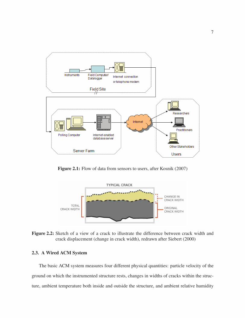
The ACM system as described above is then connected, usually via the Internet though
rarely via the public telephone network, to servers in the lab which automatically collect the
readings and make them available on a Web site. Figure 2.1 illustrates the flow of data from the
sensors to interested parties. The Internet connectivity of an ACM system also allows for remote
reconfiguration of the system operating parameters which is essential for data management of
dynamic even recording as discussed in section 2.4.1.2.
2.2. Crack Width
Siebert (2000) describes the high resolution with which the change in width of a typical
household crack must be measured (0.1 μm or 4 μin) to capture fully even its smallest changes.
This plays a significant role in the selection of the transducer to measure the crack. It is shown
in Chapter 3 the resolution requirements have a different impact on a wireless ACM system than
on a traditional, wired ACM system. Only the change in crack width is significant, as shown in
Figure 2.2.
7
Figure 2.1: Flow of data from sensors to users, after Kosnik (2007)
Figure 2.2: Sketch of a view of a crack to illustrate the difference between crack width andcrack displacement (change in crack width), redrawn after Siebert (2000)
2.3. A Wired ACM System
The basic ACM system measures four different physical quantities: particle velocity of the
ground on which the instrumented structure rests, changes in widths of cracks within the struc-
ture, ambient temperature both inside and outside the structure, and ambient relative humidity

8
both inside and outside the structure. Measurement on a single time scale of all of these quan-
tities in a given structure lends insight into the effects of both weather and nearby blasting or
construction vibration on a structure.
A typical ACM system is designed to record these physical quantities throughout a structure,
not just in one particular location. Figure 2.3 shows a scale drawing of a house in which a wired
ACM system was installed. Note that sensors are installed both indoors and outdoors, upstairs
and downstairs, and separated in some cases by over 20 feet. This type of layout is typical of
ACM systems. In the case of the system outlined in Figure 2.3, three engineers and a graduate
student spent two full days in the home of a litigant drilling holes through interior and exterior
walls, pulling cables through an attic, and gluing sensors to walls. Because this type of system
is most often installed in a home or place of business for months or years at a time, minimization
of intrusiveness and vulnerability of the ACM system is as crucial as minimization of cost and
installation time. This need to minimize simultaneously the cost, the installation time, and
the overall disruptiveness of the ACM system leads directly to the necessity of wireless ACM:
high quality instrument cable can cost several dollars per foot and must be routed discretely
through an occupied structure, avoiding sources of electromagnetic interference and hazardous
locations. Cable installation adds significantly to the time, effort, and manpower required to
install an ACM system. The existence of cables within an occupied structure also increases the
chance of intentional and unintentional damage to the cabling by the structure’s occupants.

9
Figure 2.3: Plan view of an ACM system installed in a residence, after Waldron (2006)

10
2.3.1. Crack Width Sensors
ACM systems utilize three different types of sensors to measure changes in widths of cracks.
Each of these sensors meets the precision and dynamic response characteristics required for
ACM (Siebert, 2000; Ozer, 2005). Figure 2.4 shows the three different types of crack width
sensors used for ACM: Linear variable differential transformers (LVDTs), eddy current dis-
placement gages, and string potentiometers. Table 2.1 compares the attributes of each type of
crack width sensor and can suggest which sensor should be chosen for a given measurement
scenario.
(a) (b) (c)
Figure 2.4: Photographs of three types of crack width sensors: (a) LVDT, after McKenna(2002) (b) eddy current sensor, after Waldron (2006) (c) string potentiometer, afterOzer (2005)
These three crack sensors that meet the requirements of precision and dynamic response uti-
lize significantly different physical mechanisms to measure the width of a crack. Some sensors
physically bridge the crack such that the movement of the crack can have an effect on the func-
tionality of the sensor or the existence of the crack sensor might actually affect the movement
of the crack. Other sensors do not physically bridge the crack. Sensor size, the need for signal
conditioning electronics, and cost all play a role in determining the optimal sensor for an ACM
system.
11
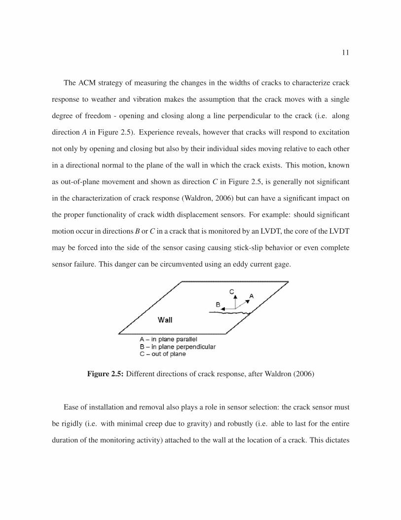
The ACM strategy of measuring the changes in the widths of cracks to characterize crack
response to weather and vibration makes the assumption that the crack moves with a single
degree of freedom - opening and closing along a line perpendicular to the crack (i.e. along
direction A in Figure 2.5). Experience reveals, however that cracks will respond to excitation
not only by opening and closing but also by their individual sides moving relative to each other
in a directional normal to the plane of the wall in which the crack exists. This motion, known
as out-of-plane movement and shown as direction C in Figure 2.5, is generally not significant
in the characterization of crack response (Waldron, 2006) but can have a significant impact on
the proper functionality of crack width displacement sensors. For example: should significant
motion occur in directions B or C in a crack that is monitored by an LVDT, the core of the LVDT
may be forced into the side of the sensor casing causing stick-slip behavior or even complete
sensor failure. This danger can be circumvented using an eddy current gage.
Figure 2.5: Different directions of crack response, after Waldron (2006)
Ease of installation and removal also plays a role in sensor selection: the crack sensor must
be rigidly (i.e. with minimal creep due to gravity) and robustly (i.e. able to last for the entire
duration of the monitoring activity) attached to the wall at the location of a crack. This dictates

12
the use of a quick-setting epoxy as described in Siebert (2000). The larger the area that needs
to be glued, the more difficult and destructive sensor removal will be.
Design of a wired ACM system typically does not need to take into account the power draw
of a given sensor type - the system has a power source (typically household 110 V AC service)
so large that power considerations are usually ignored in sensor selection. In a wireless system,
however, power is a much greater concern, as discussed in Chapter 3 and Chapter 4. Table 2.1
shows the various factors to consider when selecting a sensor for an ACM system.
LVDT Eddy Current Potentiometer
Model: DC-750-050 SMU-9000 Series 150
Approximate Cost: $250 $1700 $400
Measuring Range: ±0.05 in 0.05 in 1.5 in
Out-of-plane capable: no yes minimally a
Physically bridges crack: yes no yes
Footprint: large small b small
Power Requirements: ±15 V DC, ±25 mA 7-15 V DC, 15 mA 7 mA at 35 V DC c
Warm-up time: 2 minutes 30 minutes none
a The string potentiometer is not designed to measure motions in directions other than along the length of the
string, but experience suggests that incidental motion of this type will not damage the sensor.b The sensor itself is smaller than either of the other two types of sensors, however, the eddy current displace-
ment sensor requires signal conditioning electronics to be placed on the wall near the sensor. The enclosure
for the electronics does not, however, need to be fastened as securely (i.e. with epoxy) as the sensor itself, so
removal of the sensor and its accompanying electronics will likely do less damage to paint and plaster than
the other two displacement sensors.c The power draw of the string potentiometer is directly proportional to its input voltage; the total resistance
of the string potentiometer is 5000Ω
Table 2.1: Comparison of the attributes of three types of crack width sensors

13
2.3.2. Velocity Transducers
ACM systems make use of velocity transducers to measure two different physical phenomena:
particle velocity in the soil on which the structure is built, and the motion of the structure itself.
2.3.2.1. Traditional Buried Geophones
Particle velocity in the soil, the traditional mechanism by which mining industry regulators
restrict the effect of blasting vibration at locations away from the blast site (Dowding, 1996),
is measured using a large triaxial geophone, shown in Figure 2.6, buried in the ground near a
structure of interest. When a blast wave propagates through the soil, the geophone generates
a sinusoidal output that is observed by the ACM system at 1000 samples per second. The
ACM data logger will use this sensor’s output to trigger high-frequency recording of all relevant
sensors in the system.
Figure 2.6: Photograph of a triaxial geophone with quarter for scale

14
2.3.2.2. Miniature Geophones
In wired ACM systems, smaller geophones can be used to measure the actual motion of the
structure. These smaller geophones are single-axis devices and are therefore smaller than the
geophone in Figure 2.6. These transducers measure velocity versus time which can then be
integrated to reveal displacement versus time. If the transducers are installed at the top and
bottom of a wall section, as shown in Figure 2.7, the recorded velocity measurements can be
used to calculate the strains in the walls.
Figure 2.7: Layout of miniature geophones such that wall strains can be measured, afterMcKenna (2002)
In a wireless ACM system, these same miniature geophones can serve the purpose of pro-
viding signal by which to alert wireless nodes to the occurrence of a significant vibratory event.

15
Instead of relying on a centrally-installed geophone buried in the soil near the structure, a wire-
less system can utilize a geophone at every node to measure local vibration.
2.3.3. Temperature and Humidity Sensors
Indoor and outdoor temperature and humidity sensors, such as those shown in Figure 2.8, are
utilized to record long-term trends in temperature and humidity both inside and outside an
instrumented structure. The outdoor gage supplies useful information about the passage of
weather fronts and seasonal weather trends. The indoor gage supplies relevant information
about the activity of the furnace or air conditioning system in the house. Both data streams can
be correlated to crack response as discussed in section 2.4.1.1.
(a) (b)
Figure 2.8: Photographs of (a) indoor and (b) outdoor temperature and humidity sensors, afterWaldron (2006)
2.4. Types of Crack Monitoring
Crack behavior in response to vibration or environmental effects can manifest itself through
a number of different physical changes in the crack. The crack can elongate, open (i.e. widen)

16
and close (see direction A in Figure 2.5), shear along the axis of the crack (see direction B in
Figure 2.5), or move out-of-plane (see direction C in Figure 2.5). Measurement of each of these
types of motion can lend insight into their causes.
2.4.1. Width Change Monitoring
ACM systems are largely concerned with measurements of changes in crack widths. Though
the most serious crack activity to a homeowner might be extension or propagation of the crack
rather than opening or closing of the crack, it is reasonable to assume the driving force behind
any elongation will, in fact, be the same driving force behind widening and contracting.
Two types of phenomena exist that tend to cause changes in crack width (and therefore
possible elongation or growth of a crack). The first type, so-called long-term effects, are those
that must be measured over the periods of hours, days, months, and years in order to realize their
effect on crack behavior. The other type, so-called dynamic effects, are the motions in cracks
induced by vibration, blasting, slamming of doors, leaning against walls, and other common
household activities. These phenomena tend to be short-lived (i.e. fewer than fifteen seconds
in duration) and must be observed at a high frequency to realize their true effect on cracks.
Additionally, these dynamic phenomena cannot be expected to occur on a predictable schedule,
therefore an ACM system must be constantly aware of its sensor inputs to determine whether
such an event is occurring. A wired ACM system is able to measure both long-term and dynamic
events.

17
2.4.1.1. ACM Mode 1: Long-term
Effects that can be observed using only hourly measurements include changes in temperature
and humidity as driven by weather or the utilization of in-home heating and cooling systems or
kitchen appliances such as ovens and stoves. Measuring these effects more frequently than a
few times per hour will yield no new information about the cracks as temperature and humidity
changes are slow produce changes in crack width. To capture accurately these phenomena
and their effects on cracks, every hour the system will measure ambient indoor and outdoor
temperature, ambient indoor and outdoor humidity, and the current widths of all cracks. Though
ideally only one sample per sensor per hour is necessary to observe these long-term effects, it is
often common practice to measure average short bursts of high-frequency measurements (e.g.
sample one thousand samples for one second and average) to attempt to filter out any noise or
electromagnetic interference that may be introduced due to long cable runs.
This long-term, periodic measurement of temperature, humidity, and crack sensors is known
as Mode 1 logging and is the simpler of the two modes in which an ACM system operates. It
should be noted that readings from geophones are ignored in Mode 1 logging because slow
periodic readings from a geophone yield no useful physical information.
2.4.1.2. ACM Mode 2: Dynamic
Physical phenomenon other than temperature and humidity can have effects on cracks in the
walls of structures; the very motivation behind the development of ACM systems is to char-
acterize the effects of construction vibration and blasting on houses. These types of events
have two characteristics that make them ill-suited for recording in Mode 1. First, they can
occur at any time – one cannot assume that even the most organized construction or mining

18
operation will have a precise enough schedule of their daily activities that a system can be pre-
programmed to record at the appropriate times. Secondly, these types of events require high
frequency sampling to capture their true nature. Siebert (2000) indicates that these types of
dynamic phenomena can last for three to fifteen seconds and must be recorded at one thousand
samples per second to fully resolve all high-frequency motion.
In order to capture the entire dynamic event, some of which may occur at a time before
the peak of the input signal exceeds the trigger threshold, ACM systems utilize buffering to
avoid losing the pre-trigger data. At any given time, an ACM system has a buffer (typically one
half to a full second) of data sampled one thousand times per second stored in its memory. If
a threshold crossing condition does not occur, the data is discarded. If a crossing does occur,
however, then the pre-trigger data is concatenated to the post-trigger data to form a single time
history that clearly shows the point at which the trigger threshold was crossed.
The issue of when a dynamic event should be recorded is non-trivial. The occurrence of a
random event is determined by the data logger continuously measuring the output of a geophone
(or geophones) and using its microprocessor to compare the current geophone output to the pre-
programmed threshold value. If the threshold value is set too low, the system will be overloaded
with data that then must be transmitted back to the lab. If the value is set too high the system
will fail to record an event of interest. For this reason, remote reconfiguration of the triggering
threshold is critical for any ACM system. The best practice is to set the threshold relatively low
during system installation and testing. Should that threshold prove to generate too much data
or record events of little interest, the threshold is then slowly raised until an adequate balance is
reached.

19
This high-frequency, randomly-occurring, remotely-configurable monitoring of both geo-
phones and crack sensors is known as Mode 2 logging and is more complex to implement than
Mode 1. It should be noted that readings from temperature and humidity gages are ignored in
Mode 2 as high-frequency sampling of their data yields no useful physical information.

20
2.4.2. Crack Extension Monitoring
Though ACM systems focus on measuring changes in the width of the cracks under the assump-
tion that crack extension cannot occur without crack widening, crack propagation sensors allow
for direct measurement of the extension of a crack. Crack propagation sensors are generally
made up of a series of metallic traces of known electrical resistance. A sensor can be affixed to
the tip of a crack such that if the crack propagates, one or more of the metallic traces will break
which will change the resistance measured across the terminals of the sensor. Figure 2.9 shows
how such a sensor might function.
Figure 2.9: Resistance measured between points A and B decreases as crack propagates
This type of sensor has advantages and disadvantages over the crack width measurement
strategy of measuring crack activity. The obvious advantage of such a crack propagation sensor
is that it will directly measure the crack behavior in which a homeowner is interested: the exten-
sion of a crack. A traditional crack propagation sensor is also typically an order of magnitude
less costly than a typical crack width measurement sensor described in Section 2.3.1 above.

21
2.4.2.1. Traditional Crack Propagation Patterns
Traditional crack propagation gages are designed to be chemically bonded to a substrate that has
crack or is predicted to crack. The gages, shown in Figure 2.10 are made up of a high-endurance
K-alloy foil grid backed by a glass-fiber-reinforced epoxy matrix (Vishay Intertechnology, Inc.,
2008). Though these gages are proven to be useful in the measurement of cracking in mate-
rials such as steel or ceramic, their usefulness for measuring cracks in residential structures is
diminished due to the fact that the glass-fiber-reinforced epoxy backing is much stronger than
the drywall or plaster to which it would be affixed as part of an ACM system (Marron, 2010).
Additionally, it is not difficult to imagine that a propagating crack may alter its direction be-
fore breaking the rungs of the crack propagation gage which would render the gage ineffective.
Chapter 4 describes a method in which these sensors can be applied to steel bridges to track
progression of existing cracks.
2.4.2.2. Custom Crack Propagation Patterns
To overcome the two main difficulties inherent in using a commercially available crack propa-
gation sensor for either an ACM system or a system designed to measure cracks in steel, a new
type of crack propagation sensor is proposed in this thesis: a custom crack propagation pattern.
This pattern, detailed in Chapter 4, can be made in whatever shape is necessary for capturing
any possible direction of crack growth. It also uses the wall (or steel) to which it is mounted
as its substrate so the problem of mismatched material strengths between the substrate and the
sensor backing is eliminated.

22
Figure 2.10: Two types of commercially available crack propagation patterns shown with aquarter for scale
2.5. Examples of the output of an ACM system
The following images are taken from the live Web interface of an ACM system. Figure 2.11a
shows the long-term correlation between humidity and crack displacement as captured with
Mode 1 recording. Figure 2.11b shows typically recorded crack displacement waveforms during
a dynamically triggered event as captured with Mode 2 recording.

23
(a) (b)
Figure 2.11: Screen shots of (a) long-term correlation of crack width and humidity fromMode 1 recording (b) crack displacement waveforms from Mode 2 recording

24
2.6. Chapter Conclusion
This chapter has shown that for the purposes of monitoring crack activity as caused by vibra-
tion, mining, or weather, different types of sensors may be used to measure crack displacement.
Choice of sensor type is determined by constraints on the availability of power, precision exci-
tation, and physical space for sensor installation. By combining Mode 1 and Mode 2 recording,
the effects of long-term changes in temperature and humidity can be compared to the dynamic
effects of vibration and household activity. Both modes are essential to the true quantification
of the effects of vibration on residential structures.
This chapter has also shown that direct monitoring of crack elongation or propagation does
not require as sophisticated a data logger as does the monitoring of crack width changes with
respect to vibration, though it does require specialized crack propagation patterns.
Regardless of the chosen sensor and the makeup of a crack measurement system, the instal-
lation of any wired system is labor-intensive and expensive: high-quality instrument wires must
be run through the monitored structure: typically an occupied residence in the case of ACM
and an active highway bridge in the case of ACPS. The need to minimize installation time, cut
down on the cost and labor of installing wires, and minimize intrusiveness to the user(s) of a
structure over the course of the monitoring project clearly demonstrates the utility of wireless
monitoring systems. Chapters 3 and 4 will examine the construction of such systems.

25
CHAPTER 3
Techniques for Wireless Autonomous Crack Monitoring
3.1. Chapter Introduction
The ever decreasing size and increasing performance of computer technology suggest that
an expensive, labor-intensive, and residentially intrusive wired Autonomous Crack Monitoring
(ACM) system may be replaced by a similarly capable, easier to install, yet less expensive
and intrusive wireless ACM system based on existing, commercially available wireless sensor
networks. The implementation of a wireless ACM system with all the functions of a standard
ACM system (i.e. Mode 1 and Mode 2 recording capability), no requirement for an on-site
personal computer for system operation, a small enough footprint such that it will not disturb
the resident of the instrumented structure, a sensor suite that can be operated with minimal
power use, and system operation for at least six months without a battery change or any other
human intervention, is fraught obvious and non-obvious challenges.
3.1.1. Wireless Sensor Networks
Wireless sensor networks (WSNs) consist of a network of nodes, or “motes,” that communicate
with one or more base stations via radio links. Most WSNs transmit in the low-power, license-
free ISM (industrial, scientific, and medical) band, typically between 420 and 450 megahertz.
In general, motes are designed to be low-cost, relatively interchangeable, and in many cases,
redundantly deployed.

26
3.1.1.1. Motes
Each mote is made up of a processing unit, a radio transceiver, a power unit, and a sensing
unit. The two main components within the sensing unit are an analog-digital converter (ADC)
and software-switchable power sources to activate and deactivate sensors. The sensors, ADCs,
and switchable power supplies are either integral to the mote itself or added by means of an
external sensor board that is physically attached to the mote. In none of the WSNs described
in this thesis does any data processing occur on the motes themselves – all data is transmitted
back to the base station before any data processing might occur. For more detail on motes and
their components, see Ozer (2005). In the remainder of this document, a “mote” shall refer to
the actual processor/radio board device while a “node” shall refer to the combination of mote,
sensor board(s) external to the mote, and sensors deployed at a specific location in a structure.
3.1.1.2. Base Station
At minimum, the base station is responsible for receiving by radio all of the transmissions that
originate from within the wireless sensor network then relaying this data through some other
communication mechanism back to interested parties. In most cases, though, the base station
of a WSN contains the majority of intelligence of the system. More sophisticated base stations
have provisions for on-board data storage and analysis and provision of a control interface by
which a remote user might reconfigure the WSN after it has been deployed in the field. Some
base stations provide a Web-based interface for control of the network, provide the ability to
process and analyze data, and make available the ability to send alerts to interested parties.
Some WSN systems require this base station to be connected to a personal computer; others
support direct connection to the Internet.

27
3.1.1.3. Wireless Communication
Each mote is equipped with a radio that allows it to send and receive data to and from both
other motes and the base station. In the simplest possible WSN, each mote transmits its data
directly to the base station whenever data is available. If site conditions change such that radio
communication between the base station and the mote is no longer possible, that mote’s data is
no longer available.
More sophisticated WSNs make use of multi-hop or mesh networking with self-healing
capabilities. In this scenario, each mote has the capability of transmitting and receiving data to
and from any mote within its radio range. This ability not only extends the physical range of the
network (i.e. motes can be deployed beyond the transmission distance to the base station) but
provides alternate paths for the data to travel should an intermediary mote become damaged or
deplete its energy source. Figure 3.1 shows an example of a WSN with multi-hop capabilities.
This chapter examines both simple and sophisticated base stations, rudimentary and ad-
vanced power management strategies, and single and multi-hop network topologies.
3.1.2. Challenges of Removing the Wires from ACM
The first and most obvious challenge to the creation of a wireless ACM system is power – more
specifically: the fact that each mote is powered by a battery pack, sometimes supplemented with
a solar panel, and not by direct connection to household power lines. Because a main motivator
in the transition from wired to wireless ACM is to minimize disruption to the resident of the in-
strumented structure, frequent visits to change batteries or the use of large, high-capacity battery
packs, are unacceptable strategies to extend system longevity. Instead, the design of a wireless

28
Figure 3.1: Example of a multi-hop network: green lines represent reliable radio links betweenmotes, after Crossbow Technology, Inc. (2009b)
ACM system’s hardware and software must prioritize minimization of size but maximization of
system longevity using an energy source no larger than 2-3 standard AA batteries.
The second and relatively obvious challenge is that due to the fact that motes run on batter-
ies, it is impractical to continuously buffer data in order to monitor the readings from sensors
before a significant sensor reading triggers the system to record at a high frequency. Since there
is no way to know in advance when such a sensor reading will be needed, it becomes necessary
to continuously check the data against a known threshold. This continuous sample-compare-
buffer-discard cycle utilized by traditional ACM systems is impractical for any system based

29
on a WSN since WSNs achieve their longevity by “sleeping,” or operating in an extremely
low-power mode, for the large majority of their deployed life. In this sleeping mode, sensors
cannot be read, radio signals cannot be sent or received, and each mote is powered off with the
exception of a low-power timer that instructs it when to “wake up,” or resume a fully-functional
operating state, in order to take its next scheduled reading.
The third and somewhat less obvious challenge inherent to the transition to wireless ACM
is quality of the sensor excitation and analog-to-digital conversion capabilities of the motes.
In a state-of-the-art wired ACM system, power is supplied to the sensors by an independent
±15 V DC regulated power supply capable of supplying 0.3 A of regulated current and powered
by standard 110 V AC (SOLA HD, 2009). Analog-to-digital conversion in the state-of-the-art
wired ACM system is performed by a 16-bit analog-to-digital converter (ADC) with software-
configurable gain to allow for maximum use of the 16-bit resolution over the expected output
range of the sensor (SoMat, Inc., 2010). The wireless ACM systems examined in this chapter
have far less sophisticated power supplies and ADC units; extra effort is required to achieve the
repeatable, high-precision, high-frequency measurements required by ACM. In some cases, a
single WSN cannot meet all of these requirements in addition to the requirement of a six-month
operational lifetime with no human interaction.
Additionally, physical robustness of a wireless ACM system is not guaranteed – it depends
completely on the manufacturer and model of the WSN upon which the wireless ACM system
is built. In the case of certain types of WSNs, the end-user is responsible for fabricating an
enclosure to protect the delicate electronics of the system components.
Finally, and perhaps most importantly, few commercially available WSNs are designed for
end-user deployment – especially end users who do not possess expertise in computer science

30
or computer engineering. The hardware that composes a wired ACM system relies far less upon
the user to configure the internals of the system and instead allows a focus on exactly what is
desired to measure and the exact mechanism of measurement.
This chapter examines the process of selecting a WSN for use in a wireless ACM system,
selection of appropriate sensors for use with each type of WSN, challenges in configuration and
deployment of the systems, and the fabrication of new hardware and software techniques to en-
able a wireless ACM system to more closely duplicate the functionality of its wired counterpart.
3.2. Crack Displacement Sensor of Choice
Regardless of the which WSN is to be used as a wireless ACM system, changes in crack
width must be measured. Section 2.3.1 enumerates three different sensors that have been quali-
fied by previous researchers to adequately measure expected crack changes. Table 2.1 summa-
rizes the differences between the operating characteristics of the three candidate sensors for a
wireless ACM system.
The LVDT has the advantage in terms of sensor cost, and in a situation in which out-of-plane
motion is not expected, the LVDT shows promise for the wireless ACM application, especially
since casual observation does not reveal a significant difference in power draw between the
three sensors. The eddy current gage has a clear advantage in footprint size and crack motion
flexibility, and it even seems to draw less current than the LVDT. Closer inspection of the sensor
characteristics, however, reveals that the string potentiometer emerges as the clear choice for a
wireless ACM application.

31
The string potentiometer’s maximum power draw is 7 mA at 35 V DC. However, since
the potentiometer is a purely resistive ratiometric device, any voltage up to the manufacturer-
specified maximum of 35 V DC (Firstmark Controls, 2010) may be used to excite the sensor.
Thus, by using a lower voltage to power the device, the power consumption of the device can
be lowered significantly below that of the LVDT or the eddy current sensor.
Even if one concedes that since ACM only measures the width of a crack once per hour,
or even for a fifteen second dynamic window, the sensor will be powered off most of the time
and thus not have a significant impact on overall power draw, one must consider the warm-up
time of each device. The LVDT and eddy current gages both use complex and temperature-
dependant signal conditioning electronics to achieve their specified precision. This means that
immediately after the sensors are powered on, one must wait a certain amount of time before
an accurate reading can be taken. For the LVDT, this time is an average of 2 minutes (Puccio,
2010) while the eddy current sensor can take up to 30 minutes (Speckman, 2010) to achieve
its specified precision. Though the measurement of crack width takes only a fraction of a
second, the warm-up times of the LVDT and eddy current sensors would draw several orders of
magnitude more power than would a string potentiometer that requires no warm-up time to take
a precise measurement. Thus, the string potentiometer is the clear choice for measurements of
crack width in wireless ACM applications.
The string potentiometer, pictured in Figure 3.2, is a three-wire ratiometeric displacement
measurement sensor with a stroke length of 1.5 inches. At a position of zero inches (i.e. when
the potentiometer cable is fully retracted into its housing), the resistance measured between the
white output lead and black ground lead is 0Ω and the resistance measured between the white
output lead and red DC input lead is 5000Ω. At any cable position between fully-retracted and

32
fully-extended, the resistance measured between the white and black leads is proportional to
the distance the cable has been pulled out of its housing. To operate the sensor, a known DC
voltage is placed across the red and black leads and the voltage between the white and black
leads is measured. The distance of cable extension is the ratio of output voltage to the input
voltage times 1.5 inches. Technical specifications of the string potentiometer may be found in
Appendix B.2.
Figure 3.2: Photograph of a string potentiometer with quarter for scale, after Jevtic et al.(2007b)
Installation of the string potentiometer is accomplished using two simply fabricated alu-
minum mounting accessories. The first, a square aluminum plate with countersunk holes, is
screwed into the bottom of the string potentiometer then glued to a wall on one side of a crack.
The plate prevents epoxy from entering the housing of the potentiometer. It also provides a

33
uniform gluing surface to ensure a robust installation. The second part of the mounting fixture,
a small aluminum block with two drilled and tapped holes to accept a very thin aluminum plate
with two corresponding holes, is glued to the opposite side of the crack from the potentiometer
and grasps the measurement string. The block is sized such that the string remains parallel to
the wall. This type of fixture is preferable to a hook or a post because there is no possibility for
the string to slip or turn. Figure 3.3 shows a fully mounted string potentiometer.
Figure 3.3: Photograph of a fully mounted string potentiometer, after Ozer (2005)
3.3. WSN Selection
The WSN platform selected for the initial migration of ACM to the wireless domain was the
MICA2 wireless sensor network manufactured and sold by by Crossbow Technology Inc. and
powered by TinyOS 1.x software. The MICA2 system’s small size, flexible software, ability to
operate without a PC on site, large user base, relatively low cost, and a catalog of add-on sensor

34
boards made it the ideal choice to begin to develop a wireless ACM system. Figure 3.4 shows a
MICA2 mote with a quarter for scale.
Figure 3.4: Photograph of a Crossbow MICA2 mote with quarter for scale
3.3.1. The Mote
The MICA2 mote, Crossbow model number MPR400CB “is a third generation mote module
used for enabling low-power, wireless, sensor networks (Crossbow Technology, Inc., 2007a).”
The MICA2 features an industry-standard ATmega128L low-power microcontroller which is
powerful enough to run sensor applications while maintaining radio communication with the
base station and other motes. It also features a 10-bit ADC and a 51-pin connector and support
for several digital communication protocols for connecting to other Crossbow- and third-party-
manufactured sensor boards. Finally, it features a multi-channel radio with a nominal 500-foot

35
line-of-sight transmission range. The MICA2 arrives from the manufacturer configured to use
two standard AA-cell batteries.
The MICA2 mote is designed to operate with a Crossbow MIB510CA Serial Gatway. This
device, pictured in Figure 3.5 serves the dual purposes of acting as a programming board to
load software onto a MICA2 and acting as part of a base station that will, when paired with
an appropriately-programmed MICA2 mote, receive data from the wireless network and relay
them via RS-232 to either a local embedded field computer or directly over the Internet back to
the lab.
Figure 3.5: Photograph of a Crossbow MIB510CA serial gateway with MICA2 (without bat-teries) installed, after Ozer (2005)
3.3.2. Sensor Board Selection
Though the MICA2 mote itself features an internal 10-bit ADC, it has no ability to measure tem-
perature or humidity, nor does it have a convenient way to physically wire a sensor into its ADC;

36
note that Figure 3.4 shows no screw terminals or ADC connectors of any kind. Additionally, the
use of a 10-bit ADC on a sensor with a 1.5 inch full-scale range yields a maximum resolution
of 1465 μin – far too coarse for the expected crack width changes outlined in Section 2.2. The
MDA300CA sensor board solves all of these problems.
The MDA300CA, pictured in Figure 3.6, is a general-purpose measurement device that
can be integrated with a MICA2 mote. It is designed to be used in applications that re-
quire low-frequency measurements for agricultural monitoring and environmental controls. The
MDA300CA adds significant sensor functionality to the MICA2 board, such as a higher reso-
lution ADC and precision sensor excitation.
Figure 3.6: Photograph of a Crossbow MDA300 with quarter for scale, after Dowding et al.(2007)
In addition to its ability to measure ambient temperature and humidity without any addi-
tional hardware, the MDA300CA provides two additional capabilities:

37
3.3.2.1. Precision Sensor Excitation
Because the string potentiometer is a ratiometric sensor, its output is linearly proportional to
its input at any given instant. In order to record a precise and accurate reading from such a
sensor, the data logger must either record simultaneously the input to and the output from the
potentiometer or provide as an input to the potentiometer a precisely regulated voltage that is
guaranteed to be constant at a known value whenever the sensor is read. The MDA300CA does
the latter by providing a 2.5 V DC regulated excitation voltage to the potentiometer.
3.3.2.2. Precision Differential Channels with 12-bit ADC
The MDA300CA has several different channels with which it can read analog signals with
12-bit resolution – four times more resolution than the MICA2’s internal ADC. Four of the
MDA300CA’s channels are precision differential channels with a sensor front-end gain of 100
which yields an input range of ±12.5 mV with a constant programmable offset such that a
sensor with a minimum output of 0 V DC can still take advantage of the full 25 mV range. With
a 2.5 volt precision excitation and the front-end gain, the MDA300CA is capable of resolving
0.0061 millivolts, or approximately 3.7 μin of displacement using the string potentiometer. This
is within the specification laid out in Section 2.2. The active sensor range of the potentiometer
in the 25 mV window is 15,000 μin – 30% of the range of the eddy current gages used in the
traditional wired ACM systems (see Table 2.1) but still acceptable for ACM (Ozer, 2005). It is
important to note that although the MDA300CA is theoretically capable of resolving 3.7 μin of
movement from a string potentiometer, this assumes an environment free of all electromagnetic
interference and ambient vibration.

38
3.3.3. Software and Power Management
The MICA2 and MDA300CA, and MIB510CA compose the hardware of the wireless sensor
network. Specialized software runs on each individual MICA2 mote to control sensing, manage
transmission of data, maintain the connectivity of the mesh network if necessary, and regulate
power consumption to maximize system longevity. When software alone cannot meet all system
design specifications, hardware solutions can be employed, as in Section 3.3.6, to make the
wireless ACM system more useful.
3.3.4. MICA2-Based Wireless ACM Version 1
The first iteration of the wireless ACM system had a modest design goal: Implement Mode 1
data recording while maximizing system longevity. Version 1 did not attempt to implement
multi-hop mesh networking or sophisticated power management. It was deployed in a occu-
pied single-family home near an active limestone quarry. A traditional wired ACM system
was already installed in the home and the deployment location (an already-monitored crack in
the ceiling) was chosen to corroborate the wireless sensor readings with those taken with the
established wired system.
3.3.4.1. Hardware
Version 1 consisted of two MICA2 motes each equipped with an MDA300CA sensor board and
a single string potentiometer. An aluminum plate was attached with screws to the bottom of
each MDA300CA so that the entire mote could be affixed to the ceiling using hook-and-loop
fastener, as shown in Figure 3.7b, instead of epoxy. A nylon cable tie secured each MICA2 to
the MDA300CA because the motes were not designed to be inverted and the 51-pin connector

39
could not support the weight of a MICA2 and two AA batteries. The string potentiometer and
its cable clamp were affixed to the ceiling using the quick-setting epoxy used by Siebert (2000).
The MIB510CA with another MICA2 mote installed were located only a few feet away in a
nearby closet and attached directly to the Internet via a commercially available serial-to-Internet
Protocol gateway.

40
(a)
(b)
Figure 3.7: Photographs of Version 1 of the MICA2-based wireless ACM system, after Ozer(2005): (a) base station (in closet) (b) node (on ceiling monitoring crack)

41
3.3.4.2. Software
The application software written for Version 1 of the MICA2-based wireless ACM system was
known as MDA300Logger. The application itself and the utility applications and libraries re-
quired to make it operational are based on the example application SenseLightToLog included
with the MICA2 development kit from Crossbow. The separate publication Kotowsky (2010)
contains all of the modified source code that was used to change SenseLightToLog.
3.3.4.3. Operation
The MDA300Logger application directed each mote onto which it was installed to act as an
independent data logger that could be instructed to start and stop logging, change sampling
rate, and transmit data. A single MICA2 mote was programmed with application TOSBase
(an application provided by the manufacturer and used without modification) and inserted into
the MIB510CA base station. Instead of connecting the base station directly to a PC, the base
station was connected to a serial-to-Internet Protocol gateway that was then attached to the test
house resident’s consumer-grade cable modem. Using that gateway, a PC in the lab could issue
commands directly to each mote over the Internet.
Once the motes were installed and the Internet connection established, the user would sim-
ply use the PC to connect to each mote and instruct it to begin logging at an arbitrary interval
(e.g. once per hour). To conserve power, the MDA300Logger application would instruct the
mote to shut down five minutes after it completed taking its data readings. This five minute
period of full power would give the remote user a window in which he could retrieve a mote’s
data, change a mote’s sampling interval, or command the mote to stop logging. The user had to

42
maintain a careful record of when each mote was started and stopped such that it would known
exactly when the motes would be powered on and available to respond to commands.
An additional piece of software, the XSensorMDA300 software package included with the
development kit, was used to center the string potentiometer. An extra MICA2 mote would be
programmed with this calibration software and inserted into the MDA300CA already mounted
near the crack. When activated, this calibration mote would transmit its readings several times
per second so a PC plugged into the base station could view the real-time output of the string
potentiometer. With this live display in hand, the user could then center the string potentiometer
in the middle of its range, tighten down the screws, and replace the calibration mote with a mote
programmed with MDA300Logger.
3.3.4.4. Deployment in Test Structure
Ozer (2005) performed detailed analysis of the data that was collected using Version 1 of the
wireless ACM system. His work concluded that for during its entire operational period, lasting
from November 18th, 2004 through January 16th, 2005, the wireless ACM system based on
MDA300Logger performed similarly to a wired ACM system monitoring the same crack over
the same time period. Figure 3.8 shows that both systems measured the same general trends in
temperature and crack displacement over the two-month period.

43
Figu
re3.
8:T
emper
ature
and
crac
kdis
pla
cem
ent
mea
sure
men
tsby
wir
eles
san
dw
ired
AC
Msy
stem
sin
test
house
over
two
month
per
iod,af
ter
Oze
r(2
005)

44
From November 2004 through January 2005, the system took data once per hour. Because
of the provision of the communication window for the issuance of new commands, each mote
was fully powered-on and awaiting instructions for a full five minutes out of every hour – a duty
cycle of just over 8%. It is no surprise, then, that the system consumed all of its available battery
power in only one month (the batteries were changed in late December of 2004). Figure 3.9
shows the decline of the alkaline AA battery voltage over the time of deployment until it was no
longer sufficient to support logging and data collection halted. More detailed analysis of power
consumption can be found in Ozer (2005).
Figure 3.9: Alkaline battery voltage decline of a mote running MDA300Logger, after Ozer(2005)
3.3.4.5. Results
Version 1 of the MICA2-based wireless ACM system was largely successful. It showed that the
MICA2 combined with the MDA300CA and a string potentiometer could perform Mode 1 data

45
recording on par with a state-of-the-art wired ACM system. In spite of these positive results,
however, several improvements would still be necessary to achieve a fully-functional Mode 1
system before a Mode 2 system could be developed:
• Power management must be improved: the minimum target deployment life of a wire-
less ACM system is six months but the MDA300Logger system lasted only one.
• Data retrieval is difficult: a user of MDA300Logger must remember when data was last
uploaded to know when the next window will be available. Should the motes’ clocks
drift, the window might become difficult to find.
• The MDA300Logger system has no ability to route data through other motes. In com-
plex or RF-noisy residential environments, or in structures where the base station may
not be within radio range of all of the motes, multi-hop routing will be necessary.

46
3.3.5. MICA2-Based Wireless ACM Version 2 – XMesh
Based on the newly-released XMesh-enabled example applications developed by the WSN man-
ufacturer, Version 2 made use of largely the same hardware but an entirely different software
design to better implement Mode 1 logging. The design goal of Version 2 was to create wireless
ACM system that:
• increased system operation lifetime from one month to at least six months
• provided a more convenient operator interface
• formed a self-healing mesh network to increase both the range and the reliability of
the wireless ACM system
3.3.5.1. Hardware
Like Version 1, Version 2 consisted of several MICA2 motes equipped with MDA300CA sen-
sor boards and string potentiometers. The only hardware difference between Version 1 and
Version 2 was the replacement of the base station, which in Version 1 simply relayed packets
between a PC in the lab and the individual wireless motes, with an embedded computer. This
computer, called a Stargate Gateway and sold by Crossbow, is a fully functional GNU/Linux
computer featuring an Ethernet port, a CompactFlash slot, and a connector for a single MICA2
mote. Because the Stargate did not ship with an enclosure, it was mounted to a plastic board as
shown in Figure 3.10. Technical specifications of the Stargate may be found in Appendix B.5.
Attached to household 110 V AC power, the Stargate and the mote that was attached to it
were always powered-on and listening for data from the remote motes. The data was recorded
to the CompactFlash card where it was stored until the Stargate automatically transmitted the

47
Figure 3.10: The Stargate Gateway mounted to a plastic board
data back to the lab via the house’s high-speed Internet connection and standard Internet file
transfer protocols.
3.3.5.2. Software
After the deployment and validation of Version 1 of the MICA2-based wireless ACM system,
the WSN manufacturer released to the public a set of software libraries, XMesh, designed to
simplify power and network management of their WSNs. WSN application software written
using these software libraries automatically has the ability to create and maintain a self-healing,
multi-hop mesh network of motes. The XMesh libraries also provide advanced power manage-
ment of the sensor network as a whole to maximize system longevity.
The manufacturer also supplied a sample application, XMDA300, and a set of drivers for the
MDA300CA to demonstrate its functionality. This example software and the supplied hardware
drivers were modified to implement Mode 1 recording. Full source of all modified files can be

48
found in the separate publication Kotowsky (2010). It should be noted that the mote attached to
the base station ran the same software as did all of the remote motes. The XMDA300 software,
when installed on a mote with an identification number of zero, will automatically function as
a base station mote.
The original XMDA300 application was obtained from the manufacturer’s publicly accessi-
ble Concurrent Versions System repository in April of 2005. The majority of the modifications
took place in the main application control code, XMDA300M.nc, as the general strategy of the
application was changed. As written, the application would start the SamplerControl module,
part of the MDA300CA driver software, and allow the driver to dictate the interval at which
samples are taken. Because the available intervals were not long enough to implement Mode 1
recording, XMDA300M.nc was modified such that it has its own timer that starts and stops the
SamplerControl module, thereby putting the MDA300CA into its lowest power state when not
sampling.
The main application will start the MDA300CA, instruct it to get samples quickly, wait
for one set of readings to be completed, send those readings up the network, then completely
shut down the MDA300CA until the next sample should be read. If the MDA300CA driver
itself were responsible for managing the interval timings, the mote would never enter its lowest
power mode, severely limiting the operational lifetime. The application was built using the same
development tool chain by which the original XMDA300 application was built. The software
utilizes low-power listening mode, the second-lowest power mode that XMesh is able to provide
(Crossbow Technology, Inc., 2007e).
To facilitate ease of installation, when the motes are first turned on, the first sixty readings
are sent out once per minute. This allows the multi-hop mesh network to form (or fail to form)

49
within several minutes so that the installer has time to reconfigure the network if necessary.
Without this modification, several hours would be required to determine whether a network
layout would be functional.
3.3.5.3. Analysis of Power Consumption
To calculate the power draw of a mote using the ACM-modified version of XMDA300, a sim-
ple ammeter circuit was implemented by placing a 10-ohm resistor in series with the positive
terminal of the battery on the mote. By reading the voltage across this resistor, the current draw
of the mote can be calculated, recorded and compared to the total theoretical power capacity
of a pair of lithium AA batteries in series: 3000 mAh at 3 V DC (Energizer Holdings (2010b);
Appendix B.7). Figure 3.11 shows the current draw profile of a single mote.
The current readings were recorded at 10 hertz and averaged to determine the average cur-
rent used by the mote during a period of 18 hours. The average current draw when the mote
is sampling once per hour is 325 μA. Since the total current capacity of the battery pack is
3000 mAh, the total estimated lifespan is estimated to be approximately 384 days, assuming the
first hour of higher-frequency sampling is ignored.
3.3.5.4. Deployment in Test Structure
A deployment test of Version 2 of the MICA2-based wireless ACM system was conducted
in a century-old historic house near the Northwestern campus. The objective of the test was
to determine the degree of difficulty of the installation of the system, the effectiveness of the
XMesh routing layer to create and maintain a low-power multi-hop network, and a projection
for the true system deployment lifetime before batteries must be changed.

50
Figure 3.11: Current draw profile of a mote running the modified XMDA300 software forMode 1 recording: the periodic sampling window is shown in the dashed ovalin the inserted figure, demonstrating intermittent operation compared to ongoingoperation; after Dowding et al. (2007)
Sensor nodes were deployed throughout two structures, as shown in Figure 3.12. In the main
building, shown on the right, the Stargate base station was installed in the first floor office such
that it could be connected to the building’s high-speed Internet connection. Additional sensor
nodes were placed on each floor of the main structure: one in the basement (Figure 3.13a), one
on a sun porch on the second floor (Figure 3.13b), and one near a window in the third floor
apartment (Figure 3.13c). To increase the likelihood that the XMesh routing protocol would
form a multi-hop network, a node was placed on the second floor of the structure’s detached
garage (Figure 3.13d) some sixty feet away from the main building. Neither the sun porch nor
the garage had any insulation or climate control systems to keep their temperatures from being
affected by the outdoor temperature.

51
Figure 3.12: Distribution of sensor nodes throughout test structures
Because qualification of the string potentiometer had already been completed during the
deployment of Version 1 in parallel with a wired ACM system, the node with the string poten-
tiometer was not configured to measure a crack but instead was configured in the manner of a
“donut qualification test” as described in Baillot (2004). In this this configuration, instead of
measuring the change in width of a crack in a wall, the string potentiometer measures the ther-
mal expansion and contraction of a plastic ring, or “donut,” as shown in Figure 3.15. The node
measuring the donut was placed on the sun porch to ensure exposure to maximum temperature
differences and therefore achieve the largest possible expansion and contraction of the donut.
Finally, alkaline batteries were used in the deployment test instead of lithium batteries. Al-
though alkaline batteries have less capacity than lithium batteries, especially when operating in

52
(a) (b)
(c) (d)
Figure 3.13: MICA2-based wireless ACM Version 2 nodes located (a) in the basement, (b) onthe sun porch, (c) in the apartment, and (d) over the garage
colder temperatures (Energizer Holdings, 2010a), their voltage output decreases over time such
that the remaining battery life might be estimated. The voltage output of lithium batteries tends
to stay steady over time then drop rapidly at the end of their working capacity (Energizer Hold-
ings, 2010b). It was therefore expected that the total service life of the wireless sensor network
might decrease from the ideal estimate of 384 days to 150-200 days.

53
Figure 3.14: A typical mote in a plastic container
Figure 3.15: A string potentiometer measuring the expansion and contraction of a plastic donut

54
3.3.5.5. Results
Version 2 of the MICA2-based wireless ACM system was deployed in the test structure from
March 2006 through November 2006. Figure 3.16 shows a plot of the voltage of the batteries
versus days of deployment. Mote 2, the mote deployed in the basement, depleted its batteries
the most quickly after approximately 140 days of deployment. Mote 4, the mote deployed on
the sun porch, fared next best with a lifetime of approximately 210 days. After approximately
250 days, when the system was removed from the test structure, neither Mote 1 nor Mote 3 had
depleted its batteries.
2200
2400
2600
2800
3000
3200
3400
3600
0 50 100 150 200 250 300
Bat
tery
(mV
)
Days Deployed
Battery vs. Days Deployed
Mote 1Mote 2Mote 3Mote 4
Figure 3.16: Plot of each mote’s battery voltage versus time

55
Figure 3.17 compares the expansion and contraction of the donut with the ambient tempera-
ture. The mote with the donut was placed on the sun porch which was minimally insulated and
had no climate control.
Figures 3.18 and 3.19 compare the ambient temperature and humidity, respectively, recorded
by each mote over the deployment period. Motes 1 and 4 were deployed in environments highly
influenced by outdoor temperature, Motes 2 and 3 were deployed in climate-controlled indoor
spaces.
Along with the battery, temperature, humidity, and potentiometer readings it takes period-
ically, each mote also sends back the identity of its parent mote in the XMesh routing tree at
the time the data point is taken. The first ACM packet, i.e. a packet that contains sensor data
rather than XMesh status data, of the monitoring period came from Mote 2 at 12:00 AM on
March 23rd 2006. Between that time and the time that the last data packet was received from
Mote 2, the first mote to deplete its batteries, at 11:42 PM on August 4th 2006, 37,268 ACM
packets were received by the base station. Of these packets, 71.8% were received directly from
the mote that recorded the data – the packet “hopped” only once. Mote 1, the mote in the
garage, sent most of its data back via either Mote 3 or Mote 4, however it transmitted 16.9%
of its packets directly to the base station. Table 3.1 shows the detailed listing of motes’ parents
between the start of monitoring and the depletion of the first mote’s batteries.
3.3.5.6. Discussion
Figure 3.17 indicates that Mote 4 recorded expansion and contraction of the plastic donut that
correlated closely with temperature changes. This demonstrates that the XMesh-based ACM
software can perform Mode 1 recording.

56
1500
2000
2500
3000
3500
4000
4500
0 50 100 150 200 5
10
15
20
25
30
35
40
45D
onut
Exp
ansi
on (M
icro
inch
es)
Tem
pera
ture
(Deg
C)
Days Deployed
Donut Expansion vs. Temperature: Seasonal Change
DonutTemperature
(a)
2600
2800
3000
3200
3400
3600
3800
100 101 102 103 104 105 106 107 20
22
24
26
28
30
32
34
36
38
40
Don
ut E
xpan
sion
(Mic
roin
ches
)
Tem
pera
ture
(Deg
C)
Days Deployed
Donut Expansion vs. Temperature: Week
DonutTemperature
(b)
Figure 3.17: Plot of temperature versus donut expansion over a period of (a) 200 days and (b)one week

57
-10
0
10
20
30
40
50
60
0 50 100 150 200 250 300
Tem
pera
ture
(deg
C)
Days Deployed
Temperature vs. Days Deployed
Mote 1Mote 2Mote 3Mote 4
Figure 3.18: Plot of each Version 2 wireless ACM mote’s temperature versus time
20
30
40
50
60
70
80
0 50 100 150 200 250 300
Hum
idity
(%R
H)
Days Deployed
Humidity vs. Days Deployed
Mote 1Mote 2Mote 3Mote 4
Figure 3.19: Plot of each Version 2 wireless ACM mote’s humidity versus time

58
Transmitting Mote
Mote 1 Mote 2 Mote 3 Mote 4 Total
Pare
ntM
ote
Base 1519 (17%) 8583 (91%) 8481 (90%) 8174 (87%) 26,757 (72%)
Mote 1 – 854 (9%) 854 (9%) 853 (9%) 2561 (7%)
Mote 2 37 (≈0%) – 102 (1%) 81 (1%) 220 (1%)
Mote 3 5440 (61%) 4 (≈0%) – 309 (3%) 5753 (15%)
Mote 4 1977 (22%) 0 0 – 1977 (5%)
Total 8973 9441 9437 9417 37,268
Table 3.1: Distribution of MICA2-based wireless ACM Version 2 packets over the parents towhich they were sent
0
1
2
3
4
0 50 100 150 200 250 300
Pare
nt ID
Days Deployed
Parent vs. Days Deployed
Mote 1Mote 2Mote 3Mote 4
Figure 3.20: Plot of each Version 2 wireless ACM mote’s parent versus time

59
Figure 3.16 shows that Mote 2, the mote in the basement directly underneath the room with
the base station, depleted its battery more quickly than any other mote. Although Mote 2 is
physically closer to the base station than any of the other motes, Table 3.1 reveals that only
1% of packets from other motes were transmitted first through Mote 2 on their way to the base
station. Figure 3.20 also shows that Mote 2 did not act as a parent mote for longer than Mote
3 did. Because only 28% of the total ACM packets transmitted went through an intermediary
mote on their way to the base station and because Mote 3, after having been a parent mote for
15 times more packet transmissions as Mote 2, did not deplete its batteries, it is unlikely that
overuse as an intermediary mote caused Mote 3 to drain its batteries faster than the other motes.
Because alkaline batteries powered the motes, motes at lower temperatures would likely
have less battery longevity than motes at higher temperatures. Figure 3.18 shows ambient tem-
peratures recorded by each mote over the total deployment period. It is clear that the ambient
temperatures recorded by Mote 2 were not higher or lower than the temperatures recorded by the
other three motes, so it is unlikely that temperature played a role in the early battery depletion.
The only physical quantity that has any correlation with the early depletion of the batteries
attached to Mote 3 is ambient relative humidity. Figure 3.19 shows that the ambient relative
humidity measured in the basement of the main structure is significantly higher in the period
between days 100 and 150 than that measured by the other motes. This increased humidity may
have led to corrosion of the battery or the mote’s battery terminals which would have adversely
affected battery life. In future deployments, any negative effect of increased relative humidity
could be negated by placing the motes in sealed enclosures and applying silicone to the battery
terminals.

60
3.3.6. MICA2-Based Wireless ACM Version 3 – Shake ’n Wake
Mode 2 recording requires an ACM system to have the ability to determine whether a vibratory
event has occurred and is of sufficient magnitude to be deemed an event of interest. Tradi-
tional wired ACM systems make this determination by sampling continuously the output of
a geophone at a high frequency, typically one thousand times per second, and comparing the
sampled value to a predetermined threshold value. Should the sampled value exceed the trig-
ger threshold, the ACM system begins recording at one thousand samples per second from the
geophone and all crack displacement sensors. Figure 3.21 shows this process.
PERFORM A-DCONVERSION
COMPARE TOTHRESHOLD
BEGIN HIGHSPEED
RECORDING
Threshold Exceeded
Threshold Not Exceeded
SAMPLE INPUT
Figure 3.21: Traditional wired ACM system’s determination of threshold crossing
This process of continuous digital comparison, while possible to implement using a wire-
less sensor network, is not practical if the system is to operate for months without replacing or
recharging its batteries. The continuous process of sampling, converting the signal to a digital
value, and comparing that signal with a stored threshold value requires constant attention from

61
the control processor, signal conditioners, and analog-to-digital conversion circuitry. Imple-
mentation of Mode 2 recording with a WSN therefore required the design and fabrication of a
new hardware device to process the input from a geophone and determine whether or not it has
detected an event of interest, all without overtaxing the limited energy supply of a typical mote.
This new hardware device, Shake ’n Wake, was conceived with the following design criteria:
(1) It must not significantly increase the power consumption of a mote.
(2) It must not contaminate the output signal of its attached sensor.
(3) Its trigger threshold must be predictable and repeatable.
(4) It must wake up the mote in time to record the highest amplitudes of the motion of
interest.
Each of these criteria were proven to have been met by the Shake ’n Wake design. The
results of the experiment to verify criterion 1 are detailed in Section 3.3.7.3. The rest of the
results of the experimental verification are detailed in Appendix A.
3.3.6.1. Geophone Selection
Though the Shake ’n Wake will operate with any type of sensor that produces a voltage output,
a passive, or self-powered, sensor is necessary to realize practical power savings. A geophone, a
passive sensor that produces output voltage using energy imparted to it by the very motion that
it measures, is an ideal sensor to pair with the Shake ’n Wake. Two geophones were experimen-
tally tested with the Shake ’n Wake: a GeoSpace GS-14-L3 28 Hz 570Ω geophone, pictured
in Figure 3.22a and a GeoSpace HS-1-LT 4.5 Hz 1250Ω geophone, pictured in Figure 3.22b.
Response spectra for these geophones are supplied as Appendices B.8 and B.9, respectively.

62
To maximize the signal-to-noise ratio of the output of the geophones, shunt resistors were not
installed at the geophone output terminals.
(a) (b)
Figure 3.22: (a) GeoSpace GS 14 L3 geophone (b) GeoSpace HS 1 LT 4.5 Hz geophone
McKenna (2002) showed that the dominant frequencies of the walls and ceilings in a wide
variety of residential structures are between 8 and 15 hertz. The HS-1 geophone has a minimum
defined non-shunted response frequency of approximately 1.5 hertz and is therefore well-suited
to measuring the expected structural response. The GS-14 geophone, with a minimum defined
non-shunted response frequency of 12 hertz, is not as well suited but its smaller size makes it
more attractive for installation in an occupied residential structure.
3.3.6.2. Shake ’n Wake Design
The Shake ’n Wake board, shown in Figure 3.23, implements the same modular design and is
the same size is the commercially available sensor boards manufactured by Crossbow. It can
therefore be attached to any MICA-based wireless sensor mote by way of its standard 51-pin

63
connector. Shake ’n Wake implements the hardware portion of the Lucid Dreaming strategy for
event detection in energy constrained applications introduced by Jevtic et al. (2007a).
Because of the single-ended design of the low-power analog comparator on which the
Shake ’n Wake hardware is based, the device cannot inspect both the positive and negative
portions of any geophone output waveform using a single comparator. To avoid ignoring either
half of an input waveform, the Shake ’n Wake board has two comparators and provides the
user with two sensor input connectors: CN3 and CN4. The output leads from the geophone are
wired simultaneously to CN3 and CN4, but the connectors have opposite polarities. This wiring
ensures that both the positive and negative portions of the geophone output will be considered
in determining whether the triggering threshold is crossed.
CN3 passes its input signal directly to a comparator that compares the positive portion of
the input waveform to the user-specified threshold while ignoring the negative portion; CN4
passes the inversely polarized input signal to a second, identical comparator which compares
the negative portion of the input waveform to the threshold while ignoring the positive portion.
The same user-supplied threshold is applied to both signals. Either connector can be disabled
using the jumper switches J1 and J2. Jumper J3 provides the ability to select the interrupt
controller address on the MICA2’s processor over which the Shake ’n Wake can communicate
the occurrence of a threshold crossing, thus ensuring compatibility with other sensor boards that
might also need to interrupt the mote’s processor (Jevtic et al., 2007a).
The voltage input threshold at which the Shake ’n Wake board will wake up the mote’s
main control processor can be set in software by the user both before and after deployment
of the mote. The variability of the trigger threshold is achieved by using a programmable
potentiometer with a 32-position electronically reprogrammable wiper which is placed in series

64
Figure 3.23: The Shake ’n Wake sensor board, after Jevtic et al. (2007a)
with a precision 1.263 V DC reference and a 1 MΩ precision resister (Jevtic et al., 2007a).
Figure 3.24 shows a simplified diagram of the voltage comparison circuitry. Vcomp, the reference
voltage to which the geophone output is compared, is directly determined by the position of the
wiper, x, which is an integer between 0 and 31, inclusive. Thus, the threshold voltage to which
the input voltage is compared is:
Vcomp = 3.558 ∗ x
where Vcomp is the threshold voltage (in millivolts) and x is the setting (0-31) of the potentiome-
ter.

65
100
K
1M
(x/3
2) *
100K
(32-
x)/3
2 * 1
00K
1.26
3 vo
lts
AGN
D
R1
R2
R3
REF
Vcomp
Figure 3.24: Simplified Shake ’n Wake reference circuit diagram
3.3.7. Hardware
Like Versions 1 and 2, Version 3 consisted of several MICA2 motes equipped with MDA300CA
sensor boards, string potentiometers, and two AA batteries. Version 3 nodes also included
a single Shake ’n Wake board and a geophone. Figure 3.25 shows a photograph of a fully-
assembled Version 3 node.
The base station was significantly changed from the base station used with Version 2.
First, the Stargate was replaced with a commercially available Moxa UC-7420 RISC-based
GNU/Linux embedded computer. The Stargate was found to be too physically fragile for prac-
tical use without the creation of a fully-customized enclosure. The UC-7420 ships from the
factory in a rugged metal enclosure designed for industrial use. Because the UC-7420 was not
designed to connect to a mote via the mote’s 51-pin connector, an MIB510CA serial interface

66
Figure 3.25: Photograph of a Version 3 wireless ACM node
board was used to connect the base mote to one of the serial ports on the UC-7420. Detailed
specifications of the UC-7420 can be found in Appendix B.10.
Second, instead of relying on a locally available Internet connection to connect back to the
laboratory, the Version 3 base station includes a 3G cellular router and antenna. The inclusion
of the cellular router allows placement of the base station at any location in an instrumented
structure as long as that location has available cellular signal and 110 V AC power. Figure 3.26
shows a photograph of the base station.
Physical installation of Version 3 of the MICA2-based wireless ACM system is an extension
of Versions 1 and 2: the MICA2/MDA300CA/string potentiometer combination is mounted to
the wall in the same manner as in Version 1. The geophone, as it needs to be coupled closely
with the wall or ceiling to be monitored, requires rigid attachment to the wall using epoxy, but
the mote and sensor boards may be fastened to the wall only hook-and-loop fasteners. The HS-1

67
Figure 3.26: Photograph of the base station of Version 3 of the wireless ACM system, includingUC-7420, MIB510CA, cellular router, power distributor, and industrially-ratedhousing
geophone features a threaded protrusion for ease of installation on mechanical equipment, so
installation was made easier through the fabrication of an aluminum bracket that could accept
the protrusion and provide a flat surface for the epoxy-wall interface. Figure 3.27 shows a
Version 3 wireless ACM node installed on a wall with a string potentiometer over a crack and
an HS-1 geophone in a mounting bracket.
3.3.7.1. Software
The software portion of Version 3 of the MICA2-based wireless ACM system is an extension of
the software of Version 2 with two significant additions: the ability to allow a hardware interrupt
from an external device to bring the mote out of low-power sleep mode and the ability for each
mote to receive and relay commands broadcast from the base station. These two new features

68
Figure 3.27: Photograph of a Version 3 wireless ACM node with string potentiometer and HS-1geophone with mounting bracket installed on a wall
allow a MICA2 mote to interact with the Shake ’n Wake hardware and for a user to change
the Shake ’n Wake triggering threshold, node sampling rates, and node identification numbers
while the system is deployed.
Implementation of Version 3 required modification and cross-compilation for the UC-7420
of the xlisten and xcmd applications provided with the Crossbow MICA2 system. xcmd, the
application that allows a PC to send commands to the wireless sensor network, was modified to
allow the sending of ACM-related commands to modify sampling rates, accelerate the formation
of the mesh network, and change the triggering threshold of the Shake ’n Wake devices. xlisten,
the application that allows a PC to read data coming back from the network, was modified to
understand threshold-crossing messages and messages acknowledging receipt of commands.
This modified software can be found in the separate publication Kotowsky (2010).

69
Implementation of Version 3 also required modification of the software that runs on each
MICA2. This modification activates an interrupt request channel on the MICA2 and instructs
the mote to send back a “trigger received” message upon activation of that interrupt. The
mote will also send back its most recent data readings from the MDA300CA upon receiving
a Shake ’n Wake trigger. Additionally, the on-mote code was modified to accept the receiving
of and responding to commands from a PC. This modified software can be found the separate
publication Kotowsky (2010).
3.3.7.2. Operation
The addition of the ability to send commands to the sensor network from the base station sub-
stantially changes the installation procedure after the mote and sensors have been attached to
the structure. Rather than using a physically separate calibration mote to center the string poten-
tiometer, an engineer can center the potentiometer using only the Version 3 software. Once the
motes are powered on, the engineer can connects to the base station using any 802.11-capable
PC. He logs into the UC-7420 using secure shell and issues a command to the network to enter
quick-mesh mode in which the rate of packet transmission is significantly increased such that a
mesh network forms in under one minute instead of in 30-40 minutes. The engineer uses the
xlisten program on the UC-7420 to monitor the network output until he sees that all sensors
have acknowledged receipt of the quick-mesh command, then he issues another command to
disable quick-mesh mode. He then chooses a mote, issues a command to that mote to sample
once per second, and uses the increased sampling rate and his computer to center the string
potentiometer in the middle of its active range. He then decreases the sample rate of that mote
and moves on to the next node until all potentiometers are centered.

70
When the motes are first powered on, the trigger threshold on each Shake ’n Wake is set by
default to 31, the least sensitive setting. By issuing a command from the base station, either at
install-time or at any later time by connecting to the base station over the Internet, the trigger
threshold may be adjusted to suit the needs of the site. Table 3.2 details the ACM-related
commands that are made available with Version 3 of the MICA2-based wireless ACM software.
set rate XX is an integer [1,30].
X specifies frequency, in seconds, of ticks.
set ticks XX is an integer [1,200].
A sample is taken every X ticks.
set quick X
X is either 0 or 1.
If X is 0, the default settings for mesh formation are used.
If X is 1, the motes will transmit mesh formation information
much more quickly, allowing a mesh to me be formed quickly.
set pot XX is an integer [1,31].
X = 1 is the most sensitive.
Table 3.2: ACM-related commands added to xcmd by Version 3 of the MICA2-based wirelessACM software
3.3.7.3. Analysis of Power Consumption
To analyze the power consumption of a Shake ’n Wake-enabled mote, the simple ammeter
circuit and calculations described in Section 3.3.5.3 were utilized. Figure 3.28 shows the current
draw of a mote with Shake ’n Wake installed as compared with a Version 2 mote. Figure 3.28b
clearly indicates that during the crucial sleep-state of the mote, the current draw varies between
0.03 and 0.05 milliamps – very similar to the sleep-mode current draw of the Version 2 wireless

71
ACM system without Shake ’n Wake, shown in Figure 3.28a. Thus it can be concluded that the
Shake ’n Wake does not draw a significant amount of additional power.
Sampling
Listening and/or transmission
Sleeping (0.042 mA)
(a)
0
1
2
3
4
5
6
7
8
9
10
200 220 240 260 280 300
Cur
rent
(mA
)
Time (seconds)
Sampling andRadio Transmission 9 - 15 m A
Heartbeat1 - 2 m A
Radio Receive forMesh Maintenance 2 - 6 m A
Low Power Sleep0.030 - 0.050 m A
(b)
Figure 3.28: Current draw of (a) wireless ACM Version 2 mote with no Shake ’n Wake, afterDowding et al. (2007) (b) Version 3 mote with Shake ’n Wake

72
3.3.7.4. Deployment in Test Structure
A deployment test of Version 3 of the MICA2-based wireless ACM system was conducted in the
main building of the test structures near the Northwestern campus described in Section 3.3.5.4
between September 2007 and February 2008. The objective of the test was to determine the
degree of difficulty of the installation of the system, the effectiveness of the Shake ’n Wake
in detecting vibration events, and further assurance that Shake ’n Wake does not significantly
decrease deployment lifetime of the system.
Sensor nodes were deployed through only one of the structures, as shown in Figure 3.29.
Two geophone-only nodes (with no MDA300CA or string potentiometer) were installed on
the underside the service stairway leading from the basement to the kitchen, as pictured in Fig-
ure 3.30a. One of these motes was connected to a GS-1 geophone, the other was connected to an
HS-1 geophone. Two motes, each equipped with a MDA300CA sensor board, a Shake ’n Wake
sensor board, an HS-1 geophone in a mounting bracket, and a string potentiometer were in-
stalled over existing cracks in the structure: one over the doorway leading from the kitchen into
the service stairway to the second floor, shown in Figure 3.30b, and one on the wall of the main
stairway leading from the second floor to the third floor, shown in Figure 3.30c. These two
motes were installed alongside optical crack measurement devices used for a different project.
The base station, shown in Figure 3.30d, was deployed in the basement underneath the kitchen.
3.3.7.5. Results
Figure 3.31 shows plots of temperature, humidity, battery voltage, and parent mote over the
entire deployment period. Only Motes 3 and 4 transmit this data – they are the only motes with
an MDA300CA attached. The plots indicate that after approximately 25 days of deployment,

73
Figure 3.29: Layout of nodes in Version 3 test deployment
the system ceased to take data. Later examination indicated that this failure was due to an un-
foreseen software condition that caused the monitoring to stop prematurely. At approximately
day 75, a workaround was implemented: each night, the base station would automatically re-
broadcast the correct sampling interval. Data transmission was restored immediately. Mote 4
ceased taking data between days 85 and 115 for a reason that is not yet understood but thought
to be an issue with the mesh networking protocol – Figure 3.31d shows that Mote 4 used Mote 3
as an intermediary, which was the only difference between those motes.

74
(a) (b)
(c) (d)
Figure 3.30: Version 3 wireless ACM nodes located (a) on the underside of the service stairs(b) over service stair doorway to kitchen, and (c) on the wall of the main stairway– (d) the base station in the basement
Diagnostic logs on the base station showed that Motes 1 and 2, the motes underneath the
service staircase with no MDA300CA sensor boards, did not reply when the sampling interval
workaround was implemented near day 75. The most reasonable explanation for this behavior
is that the lack of MDA300CA attached to these motes caused the XMesh power management
algorithm to fail causing the batteries to deplete after only two days, approximately the same
expected lifetime of a MICA2 with no power management. Figure 3.31d does show that Mote 1
was functioning as a parent mote for Mote 3 before it failed.

75
5
10
15
20
25
30
0 20 40 60 80 100 120 140 160
Tem
pera
ture
(deg
C)
Days Deployed
Temperature vs. Days Deployed
Mote 3Mote 4
(a)
10
20
30
40
50
60
70
0 20 40 60 80 100 120 140 160
Hum
idity
(%R
H)
Days Deployed
Humidity vs. Days Deployed
Mote 3Mote 4
(b)
0
500
1000
1500
2000
2500
3000
3500
0 20 40 60 80 100 120 140 160
Bat
tery
(mV
)
Days Deployed
Battery vs. Days Deployed
Mote 3Mote 4
(c)
0
1
2
3
4
0 20 40 60 80 100 120 140 160
Pare
nt ID
Days Deployed
Parent vs. Days Deployed
Mote 3Mote 4
(d)
Figure 3.31: Plots of (a) temperature (b) humidity (c) battery voltage and (d) parent mote ad-dress recorded by Version 3 of the wireless ACM system over the entire deploy-ment period
Figure 3.32 shows the data recorded over the period from day 75, when the base station
workarund was implemented, through the time the system was removed from the test structure.
Figure 3.32d shows when a Shake ’n Wake trigger signal was received at Motes 3 or 4.

76
5
10
15
20
25
30
80 90 100 110 120 130 140 150
Tem
pera
ture
(deg
C)
Days Deployed
Temperature vs. Days Deployed
Mote 3Mote 4
(a)
10
15
20
25
30
35
40
45
50
55
80 90 100 110 120 130 140 150
Hum
idity
(%R
H)
Days Deployed
Humidity vs. Days Deployed
Mote 3Mote 4
(b)
-5000
-4000
-3000
-2000
-1000
0
1000
2000
3000
80 90 100 110 120 130 140 150
Cra
ck E
xpan
sion
(mic
roin
ches
)
Days Deployed
Motes 3 and 4 Crack Expansion vs. Days Deployed
Mote 3Mote 4
(c)
0
1
80 90 100 110 120 130 140 150
Trig
ger
Days Deployed
Impacts vs. Days Deployed
Mote 3Mote 4
(d)
Figure 3.32: Plots of (a) temperature (b) humidity (c) crack displacement and (d)Shake ’n Wake triggers recorded by the Version 3 of the wireless ACM systemover the 75-day period of interest
3.3.7.6. Discussion
Figure 3.31c shows the alkaline battery voltage versus deployment time for Version 3 of the
MICA2-based ACM system. Figure 3.33 compares the battery voltage versus time of Ver-
sions 2 and 3 of the two MICA2-based wireless ACM systems. The two Version 3 motes with
MDA300CA boards installed lasted approximately 150 days. The graph indicates, however,
that battery voltage decay curve of the more economical batteries used in Version 3 did not

77
match those used in Version 2. This evidence, added to the similar current consumption pro-
files shown in Figure 3.11, indicates that Version 3 can operated for at least six months when
high-quality alkaline batteries are used.
2000
2200
2400
2600
2800
3000
3200
3400
0 50 100 150 200 250 300
Bat
tery
(mV
)
Days Deployed
Battery vs. Days Deployed
Mote 3 (Version 3)Mote 4 (Version 3)Mote 1 (Version 2)Mote 2 (Version 2)Mote 3 (Version 2)Mote 4 (Version 2)
Figure 3.33: Comparison of battery voltage versus time for the Version 2 and Version 3 wirelessACM systems
Figure 3.32c shows that the MDA300CA reported what appear to be three different sets
of string potentiometer readings, each separated by an approximately 1800 μin pseudo-constant
offset. In post processing, it is possible to filter the three sets of data into three regions, as shown
in Figure 3.34, under the assumption that each region represents the same physical reading with
constant 1800 μin offsets. 84% of the data points fall into the region with an absolute value
above 760 μin. The high region, as outlined Table 3.3, contains the majority of the recorded

78
points. Figure 3.35 shows plots of temperature and humidity versus the high region of measured
crack width.
-4000
-3000
-2000
-1000
0
1000
2000
3000
80 90 100 110 120 130 140 150
Cra
ck E
xpan
sion
(mic
roin
ches
)
Days Deployed
Mote 3 Crack Expansion vs. Days Deployed (filtered)
LowMid
High
Figure 3.34: Plot of three separate sets of crack width data as recorded by Mote 3 of the Ver-sion 3 wireless ACM system
Points Recorded Percentage Bounds (mV) Bounds (μin)
High 4634 84% > 1.9mV > 760 μin
Mid 736 13% 1.9mV > y > −2mV 760 μin > y > −800 μin
Low 160 3% < −2mV < −800 μin
Table 3.3: Results of filtering Version 3 wireless ACM potentiometer readings
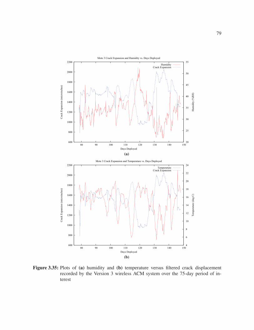
79
600
800
1000
1200
1400
1600
1800
2000
2200
80 90 100 110 120 130 140 150 20
25
30
35
40
45
50
55C
rack
Exp
ansi
on (m
icro
inch
es)
Hum
idity
(%R
H)
Days Deployed
Mote 3 Crack Expansion and Humidity vs. Days Deployed
HumidityCrack Expansion
(a)
600
800
1000
1200
1400
1600
1800
2000
2200
80 90 100 110 120 130 140 150 4
6
8
10
12
14
16
18
20
22
24
Cra
ck E
xpan
sion
(mic
roin
ches
)
Tem
pera
ture
(deg
C)
Days Deployed
Mote 3 Crack Expansion and Temperature vs. Days Deployed
TemperatureCrack Expansion
(b)
Figure 3.35: Plots of (a) humidity and (b) temperature versus filtered crack displacementrecorded by the Version 3 wireless ACM system over the 75-day period of in-terest

80
3.3.8. Wireless ACM Conclusions
This chapter has described three versions of a wireless ACM system built on the MICA2 plat-
form. Version 1 was a proof-of-concept designed to demonstrate the viability of a MICA2-based
implementation of ACM by implementing Mode 1 recording. Version 2 incorporated new wire-
less mesh networking and power management libraries to implement Mode 1 recording with
more reliability and system longevity. Version 3 incorporated the design and manufacture of
a new sensor board, the Shake ’n Wake, to allow data to be taken at random times rather than
scheduled times without sacrificing system longevity. The following conclusions can be drawn:
• The MICA2 WSN platform combined with MDA300CA sensor boards and string po-
tentiometers is capable of performing Mode 1 recording for approximately 30 days.
The MDA300CA is essential as the internal ADC on the MICA2 does not have suffi-
cient resolution or front-end gain for the expected potentiometer output.
• Intelligent power management software based on the XMesh routing layer can be
used with the MICA2/MDA300CA/potentiometer system to operate a fully functional
Mode 1 system for six to twelve months.
• Battery longevity is is dependant on the ambient temperature and humidity of the de-
ployment environment.
• A robust, industrially-rated and fully enclosed GNU/Linux embedded computer can be
combined with an MIB510CA board to create a reliable and secure Internet-accessible
base station that can continue to collect data even while the Internet connection might
be off-line. Such a base station can also be used to modify the WSN operating param-
eters, either automatically or on demand.

81
• The inclusion of a cellular modem in the base station allows a MICA2-based ACM
system to be deployed anywhere with 110 V AC power within radio range of the sensor
network.
• Installation time is decreased with the added ability to put the motes into quick-mesh
mode to form the initial mesh network. Installation is further simplified by the added
ability to individually increase the sampling rate of a mote in order to more easily
center the string potentiometer over a crack.
• Shake ’n Wake adds the ability for a MICA2-based wireless ACM mote to respond to
a randomly occurring event of interest without sacrificing power.
• A MICA2-based wireless ACM node should not be deployed without a MDA300CA
sensor board, even if the node does not need to measure the width of a crack.
• The MDA300CA board and its drivers prevent the MICA2-based ACM system from
fully implementing Mode 2 recording, even when paired with Shake ’n Wake, as its
drivers do not fully support sampling rates of 1000 hertz.
• Installation of a string potentiometer would be made less difficult if the MDA300CA
had a software-programmable front-end gain; the active range of the potentiometer
decreases by 99% due to the front-end gain on the MDA300.
• Software incompatibilities between the MDA300CA drivers and the Shake ’n Wake
drivers cause the MDA300CA to take readings from the string potentiometer with a
DC offset approximately 15% of the time. These anomalous readings can be filtered
out in post-processing.
• The Shake ’n Wake hardware design and a software implementation of the Lucid
Dreaming strategy for random event detection in energy-constrained systems are not

82
uniquely compatible with the MICA2-MDA300CA system described in this chapter;
they can be ported to any wireless sensor network that allows for direct physical ac-
cess to the interrupt lines on the control processor and proper access to the low-level
software. Unfortunately, many commercially available systems designed for ease of
use for novice users do not provide such access, thus Shake ’n Wake/Lucid Dreaming
integration must be performed at the factory and not by the end user.

83
CHAPTER 4
Techniques for Wireless Autonomous Crack Propagation Sensing
4.1. Chapter Introduction
Autonomous Crack Propagation Sensing (ACPS) is a measurement technique designed to
record the propagation of slow-growing structural cracks over long periods of time. In contrast
to ACM, ACPS, does not seek to directly correlate crack extension to any other physical phe-
nomena; rather ACPS seeks to record quantitatively, repeatably, and accurately the extension of
cracks in structures, specifically to supplement regular inspections of bridges. An ACPS system
allows structural stakeholders to be alerted to crack extensions with ample time to ensure the
safety of the structure and those using it.
Though ACPS techniques can be applied to any structure that exhibits cracking over time,
the primary motivation in the development of this technique is to supplement the in-service
inspection of fatigue cracks in steel bridges. Fatigue cracks in steel, such as those shown in
Figure 4.1, tend to grow slowly over time, and when found during routine inspection of steel
bridges, are cataloged according to procedures laid out in the Bridge Inspector’s Reference
Manual, or BIRM (United States Department of Transportation: Federal Highway Administra-
tion, 2006). These cracks are then re-examined at the next inspection and compared to records
to determine whether the crack has grown.
ACPS, especially on bridges, is an ideal application for a wireless sensor network. Run-
ning wires across bridges between different points of interest is usually cost-prohibitive and is

84
often impossible due to superstructure configuration and access restrictions. Since access can
be difficult and expensive, it is desirable to minimize installation time and maximize time be-
tween maintenance visits, so long-lasting solar-powered nodes are ideal. Furthermore, power
management strategies implemented by the manufacturers of existing wireless sensor networks
are well-suited to the low sampling rate required by ACPS.
4.1.1. Visual Inspection
Visual inspection is the most common mechanism by which the growth of cracks is recorded
quantitatively. By federal law, every bridge in the United States over 20 feet in length must be
inspected at least once every two years by specially trained bridge inspectors. This inspection
frequency can be increased based on the design, past performance, or age of the bridge. A
key part of these routine bridge inspections is identification of fatigue cracks, or cracks due to
cyclic loading, in steel bridge members. These cracks tend to grow slowly over time depending
on the volume of truck traffic, load history, weld quality, and ambient temperature (United States
Department of Transportation: Federal Highway Administration, 2006).
Fatigue cracks are commonly cataloged by recording the method by which they were dis-
covered, date of discovery, crack dimensions, current weather conditions, presence of corrosion,
and other factors that may contribute to the form or behavior of the crack. The BIRM indicates
that the inspector should: “Label the member using paint or other permanent markings, mark
the ends of the crack, the date, compare to any previous markings, be sensitive to aesthetics
at prominent areas. Photograph and sketch the member and the defect.” Figure 4.2 shows an
example from the BIRM of how a fatigue crack should be marked.

85
Figure 4.1: Fatigue crack at coped top flange of riveted connection, after United States Depart-ment of Transportation: Federal Highway Administration (2006)
Figure 4.2: Fatigue crack marked as per the BIRM, after United States Department of Trans-portation: Federal Highway Administration (2006)

86
The tracking of crack growth by visual inspection has several drawbacks, the most obvious
of which is that documentation of the conditions of cracks can only be updated during inspec-
tions which may occur as infrequently as once every two years. Less obviously, photographic
records of crack length tend not to be repeatable due to changes in photography angle, ambient
light, photographic equipment, and inspector.
4.1.2. Other Crack Propagation Detection Techniques
Several other techniques exist for the detection, classification, and monitoring of fatigue crack-
ing in structures. Acoustic emission monitoring, as described in Hopwood and Prine (1987) can
be used to determine whether a crack is actively growing or has extinguished itself. Stolze et al.
(2009) describe a method to detect and monitor the progression of cracks using guided waves.
ACPS with wireless sensor networks has several distinct advantages over these structural health
monitoring techniques when applied to in-service bridges:
• ACPS is designed to be deployed for months or years on an actively utilized structure.
The other techniques are not designed to be used in the field for more than a few days.
• ACPS using commercially available wireless sensor networks is an order of magnitude
less expensive than acoustic emission or guided wave equipment.
• ACPS sensors on a wireless network do not require power or signal cables to be in-
stalled on a bridge.
• ACPS using a wireless sensor network may not require special software or program-
ming skills.
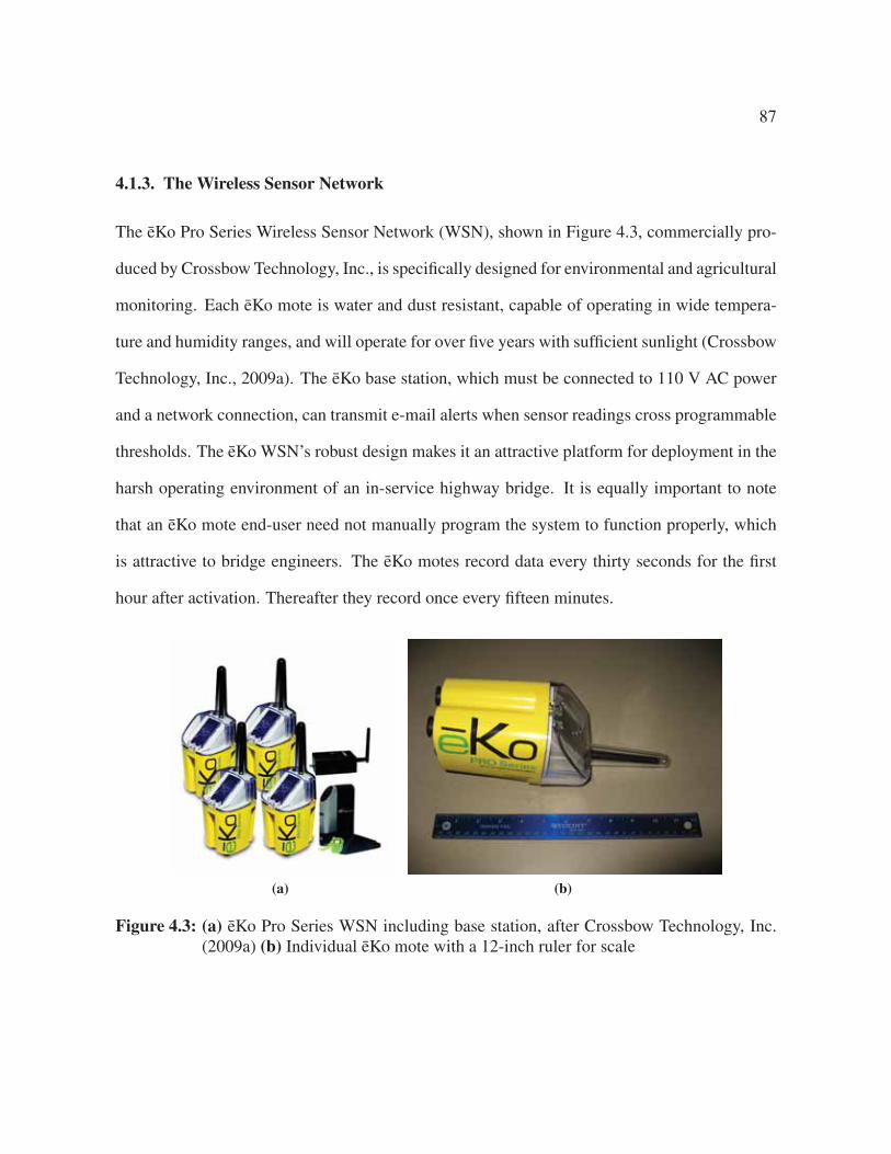
87
4.1.3. The Wireless Sensor Network
The eKo Pro Series Wireless Sensor Network (WSN), shown in Figure 4.3, commercially pro-
duced by Crossbow Technology, Inc., is specifically designed for environmental and agricultural
monitoring. Each eKo mote is water and dust resistant, capable of operating in wide tempera-
ture and humidity ranges, and will operate for over five years with sufficient sunlight (Crossbow
Technology, Inc., 2009a). The eKo base station, which must be connected to 110 V AC power
and a network connection, can transmit e-mail alerts when sensor readings cross programmable
thresholds. The eKo WSN’s robust design makes it an attractive platform for deployment in the
harsh operating environment of an in-service highway bridge. It is equally important to note
that an eKo mote end-user need not manually program the system to function properly, which
is attractive to bridge engineers. The eKo motes record data every thirty seconds for the first
hour after activation. Thereafter they record once every fifteen minutes.
(a) (b)
Figure 4.3: (a) eKo Pro Series WSN including base station, after Crossbow Technology, Inc.(2009a) (b) Individual eKo mote with a 12-inch ruler for scale

88
4.2. ACPS Using Commercially Available Sensors
Direct measurement of the elongation of a crack can be measured with a crack propagation
pattern, a brittle, paper-thin coupon on which a ladder-like pattern of electrically conductive
material is printed. This coupon is glued to the surface of the material at the tip of the crack, as
shown in Figure 4.4. When the crack elongates and breaks the rungs of the pattern, the electrical
resistance between the sensor’s two terminals will change. This resistance is be read using an
eKo mote to record the distance the crack has propagated.
Figure 4.4: Cartoon of a crack propagation pattern configured to measure the growth of a crack:resistance is measured between points A and B.
Vishay Intertechnology, Inc. manufactures commercially a series of these crack propaga-
tion patterns. Two of these sensors were chosen for use in an ACPS system: the TK-09-CPA02-
005/DP, or “narrow gage,” shown in Figure 4.5a and the TK-09-CPC03-003/DP, or “wide gage,”
shown in Figure 4.5b. Both sensors allow for the measurement of twenty distinct crack lengths

89
with their twenty breakable grid lines. The narrow gage’s grid lines are spaced 0.02 inches apart,
while the wide gage’s grid lines are spaced 0.08 inches apart. Additionally, the narrow gage’s
resistance varies non-linearly with the number of rungs broken, as shown in Figure 4.6a, while
the wide gage’s resistance varies linearly with number of rungs broken, as shown in Figure 4.6b.
This linear behavior occurs because each rung of the wide gage has a resistance specifically de-
signed such that when it is broken, the change in the overall resistance of the sensor is linear, not
exponential. The narrow gage’s rungs are all approximately the same width and therefore have
the same resistance. This behavior becomes significant when signal resolution is considered in
Section 4.2.1.
(a) (b)
Figure 4.5: Crack propagation patterns (a) TK-09-CPA02-005/DP (narrow) (b) TK-09-CPC03-003/DP (wide)
4.2.1. Integration with Environmental Sensor Bus
The eKo Pro Series WSN is designed to be used with sensors that communicate over Cross-
bow’s Environmental Sensor Bus (ESB). The ESB protocol (Crossbow Technology, Inc., 2009c)

90
(a) (b)
Figure 4.6: Crack propagation resistance versus rungs broken for (a) TK-09-CPA02-005/DP(narrow) (b) TK-09-CPC03-003/DP (wide), after Vishay Intertechnology, Inc.(2008)
describes a specific connector type, power supply, and digital interface scheme that must be im-
plemented by the sensor manufacturer if that sensor is to be used with an eKo mote. The crack
propagation patterns are not compliant with the ESB, so a customized interface cable was de-
signed, built, and installed.
The custom interface cable is composed of a Maxim DS2431 1024-Bit 1-Wire EEPROM,
a Switchcraft EN3C6F water-resistant 6-conductor connector, a length of Category 5e sold-
conductor cable, one 374Ω precision resistor and one 49.9Ω precision resistor. The EEPROM
was soldered into the water-tight connector housing as shown in Figure 4.7. The EEPROM
allows a sensor to respond with a unique sensor identifier when queried by an eKo mote such
that the sensor will be properly identified and configured automatically by any mote to which
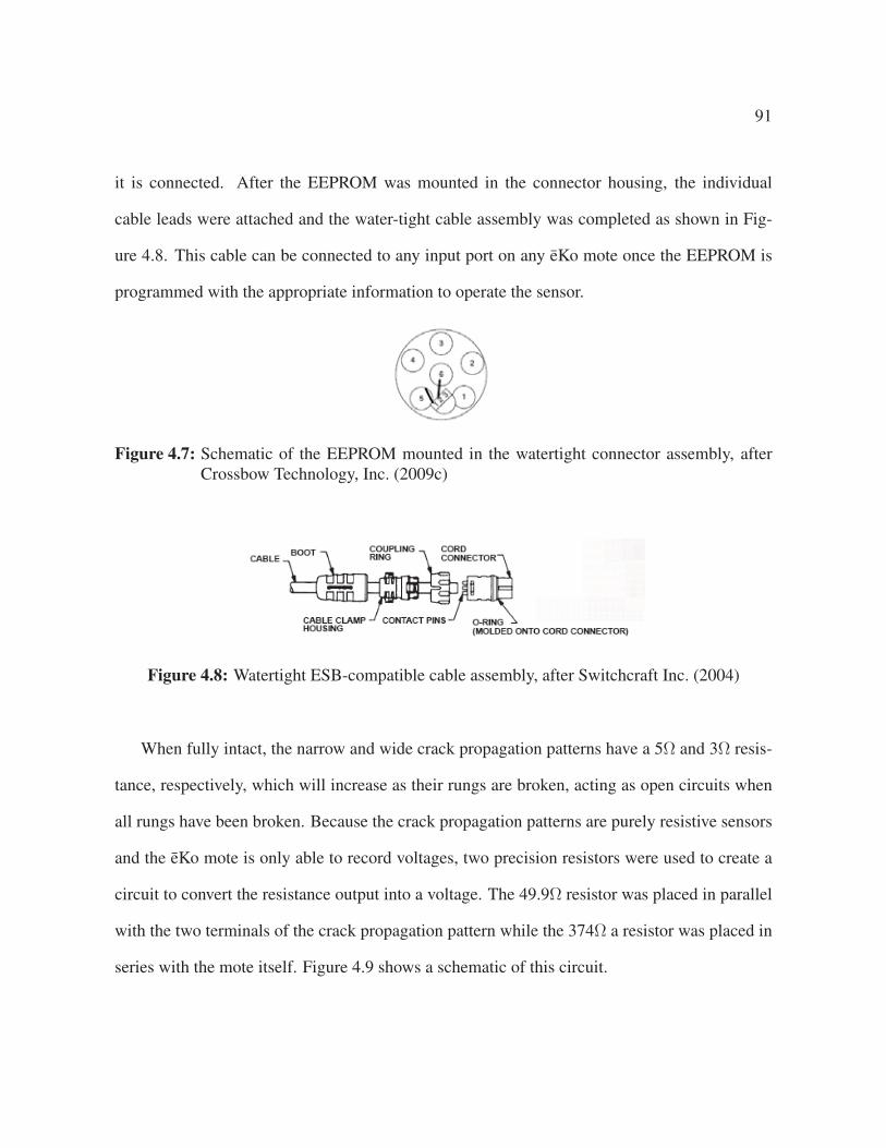
91
it is connected. After the EEPROM was mounted in the connector housing, the individual
cable leads were attached and the water-tight cable assembly was completed as shown in Fig-
ure 4.8. This cable can be connected to any input port on any eKo mote once the EEPROM is
programmed with the appropriate information to operate the sensor.
Figure 4.7: Schematic of the EEPROM mounted in the watertight connector assembly, afterCrossbow Technology, Inc. (2009c)
Figure 4.8: Watertight ESB-compatible cable assembly, after Switchcraft Inc. (2004)
When fully intact, the narrow and wide crack propagation patterns have a 5Ω and 3Ω resis-
tance, respectively, which will increase as their rungs are broken, acting as open circuits when
all rungs have been broken. Because the crack propagation patterns are purely resistive sensors
and the eKo mote is only able to record voltages, two precision resistors were used to create a
circuit to convert the resistance output into a voltage. The 49.9Ω resistor was placed in parallel
with the two terminals of the crack propagation pattern while the 374Ω a resistor was placed in
series with the mote itself. Figure 4.9 shows a schematic of this circuit.

92
Figure 4.9: Diagram of sensor readout circuit, adapted from Vishay Intertechnology, Inc.(2008)
This circuit can be connected to either the narrow or wide gage, and will cause each rung
break of a wide pattern to register an increase of approximately 10 millivolts on the eKo mote.
Because the resistance change is so small, the first rung breaks of a narrow sensor will register
no measurable voltage difference on the eKo mote, but the last several rungs broken will register
a significantly higher voltage change than the rungs of a wide gage. The circuit was placed
within the custom cable so that two exposed leads at the opposite end of the cable from the
watertight connector may be soldered to the two terminals of the crack propagation pattern after
it has been mounted on the target material.
In addition to the fabrication of the custom ESB interface cable, a customized data inter-
pretation file for each type of crack propagation sensor was created and stored on the eKo base
station. These files, found in the separate document Kotowsky (2010), need only to be created
once by the sensor manufacturer and do not need to be created or maintained by the end-user of
the ACPS system.

93
4.2.2. Proof-of-Concept Experiment
A proof-of-concept experiment was designed to test both the effectiveness of the crack propa-
gation gages in measuring fatigue cracking in steel and the eKo motes’ ability to reliably and
accurately read the sensors. Three 3.5 in by 3.5 in by 0.5 in ASTM E2472 compact tension test
coupons A, B, and C, a schematic of which is shown in Figure 4.10, were fabricated from A36
steel. These coupons were placed in a mechanical testing apparatus to apply cyclic tensile forces
at their circular attachment points to propagate a crack through the specimens and the gages.
Before each coupon was instrumented with a crack propagation pattern, a fatigue crack was
initiated in each one under the assumption that any crack to be instrumented in the field would
have begun to grow before the sensor is affixed. During the pre-cracking procedure, the relative
displacement of the attachment points was cycled between 0.24 inches and 0.0016 inches at a
frequency of 10 hertz until a crack was observed to be growing from the tip of the wire-cut
notch. Approximately 10,000 cycles were required to initiate crack growth.
Coupon A was instrumented with a narrow crack propagation pattern on one face, as shown
in Figure 4.11a. Coupon B was instrumented with a wide crack propagation pattern on one face,
as shown in Figure 4.11b. The wide pattern was too long to fit on the test coupon, so the three
rungs farthest away from the crack tip were removed before testing. The initial reading would
therefore indicate three rungs already having been broken before crack propagation began.
The crack propagation patterns on both Coupons A and B were affixed using the manufac-
turer’s recommended solvent-thinned adhesive cured at a temperature of at least +300 ◦F. This
elevated temperature cure is not practical in the field, so Coupon C was instrumented with a
narrow pattern on one face and a wide pattern on the other face using epoxy cured at room
temperature to determine if this would have a detrimental effect on ACPS functionality.

94
Figure 4.10: Schematic of compact test specimen: W=3.5 in, B=0.5 in, after for Testing andMaterials (2006)
(a) (b)
Figure 4.11: Test coupon with (a) narrow gage and (b) wide gage installed
4.2.2.1. Experimental Procedure
After the fatigue cracking procedure was performed and the gages were affixed to the coupons,
each coupon was loaded into the mechanical testing machine and wired to either an eKo mote in

95
the case of Coupons A and B, or a general-purpose data logger and bench-top power supply in
the case of Coupon C. The experiments on coupons A and B were designed to verify function-
ality of both the gages and the eKo motes, but the experiment on Coupon C was designed solely
to verify the performance of the sensor adhesion procedure. Figure 4.12 shows a photograph of
the experimental setup.
Figure 4.12: Photograph of experiment configuration for pre-manufactured crack propagationgages
During the approximately 80-minute tests, the coupons were cyclically loaded between
0.07 kip and 2.5 kip at decreasing frequencies. The crack in Coupon A propagated through
all twenty rungs of the narrow gage, as shown in Figure 4.13a, while the crack in Coupon B
propagated through eight rungs of the wide gage, as shown in Figure 4.13b.

96
(a) (b)
Figure 4.13: Test coupons with crack propagated through (a) narrow gage and (b) wide gageaffixed with elevated-temperature-cured adhesive
Coupon C was subjected to the same testing procedure as were Coupons A and B, but the
testing was aborted when it was observed that the room-temperature-cured adhesive had failed
before the gage itself, as shown in Figure 4.14.
Figure 4.14: Photograph of glue failure on wide gage affixed with room temperature-curedadhesive: the indicated region shows the glue failed before the gage.

97
4.2.3. Results and Discussion
0
0.05
0.1
0.15
0.2
0.25
0.3
0.35
0 500 1000 1500 2000 2500 3000 3500 4000 4500 5000
Sens
or R
eadi
ng (V
)
Elapsed Seconds
Coupons A and B
Narrow - Coupon AWide - Coupon B
Figure 4.15: Data recorded by eKo mote during tests of Coupons A and B
Figure 4.15 shows the data recorded by an eKo mote during tests of Coupons A and B.
The wide gage showed a linear change of voltage versus number of broken rungs. Eight rung-
breaks are easily identifiable. The narrow gage showed a non-linear change of voltage versus
number of broken rungs. Figure 4.13a clearly indicates that all twenty rungs have been broken
by the crack, but Figure 4.15 only shows ten discernible increases in voltage. This result is not
unexpected: the 10-bit analog-to-digital conversion unit and the 3 V DC precision excitation
voltage on the eKo mote combine to limit the minimum-viewable change in voltage output of
any sensor to approximately 3 mV. This resolution is suitable for measuring a rung-break on the
wide gage but it is not suitable for measuring the breakage of the first 10-12 rungs of the narrow

98
gage. Figure 4.6a shows that the resistance change exhibited by a narrow gage for the first 10-12
rung-breaks is significantly lower than that for the last 8-10 rung-breaks, therefore the voltage
change exhibited by the readout circuit will also be lower for the first 10-12 rung-breaks.
Two times over the course of the test, the eKo mote read momentary jumps in the voltage
output of the wide gage and its readout circuit. This same phenomenon was observed eleven
times with the narrow gage. This behavior is explained by noting that for any voltage input to the
eKo mote’s analog-to-digital conversion unit that falls on or near one of the 3 mV thresholds, a
small amount of electromagnetic interference is capable of increasing or decreasing the voltage
of the observed signal such that it could appear to have fallen into either of the two adjacent
conversion regions. It is also possible that since the crack, and therefore the conductive portions
of the gage, were loaded cyclically, intermittent contact may occur just before or after a rung
had been broken.
Figure 4.14 shows that the adhesive cured at room temperature was not able to withstand the
cyclic strains imposed by the fatigue test. The lightly colored region indicated in Figure 4.14
shows where the adhesive holding the gage to the steel coupon has released and allowed air to
fill the gap between the coupon and the substrate of the crack propagation gage. Once the brittle
substrate of the gage separates from the surface on which it is mounted, the gage will not only
fail to reflect accurately the position of the crack tip beneath it, but it will become extremely
fragile and likely to fail due to some other physical phenomenon than crack propagation.
4.3. Custom Crack Propagation Gage
An implicit assumption made in the use of crack propagation gages such as those described
in Section 4.2.2 is that the engineer has a priori knowledge at the time of sensor installation of

99
the direction in which the crack is going to propagate. In cases where such knowledge does
not exist, several of these mass-produced gages would be necessary to track the crack in all of
its possible propagation directions. Additionally, the results of the experiment on Coupon C
in Section 4.2.2 indicated that for the best results, an impractical installation method involving
elevated-temperature-cured adhesive must be employed to utilize these gages.
A solution to both of these problems is a so-called custom crack propagation gage. This
type of gage is drawn, rather than glued, near the crack to be monitored, using commercially
available conductive material. This material, combined with a more sophisticated network of
signal conditioning resistors, creates a gage that can be any shape or size.
4.3.1. Theory of Operation of Custom Crack Propagation Sensor
The basic principles on which custom crack propagation gages function are similar to their pre-
fabricated counterparts: an existing crack in a structure grows, propagating over time through
one or more rungs of the sensor. As each rung breaks, the resistance of the entire sensor in-
creases by a known value. Using a precision excitation voltage and precision resistors of a
known value, each rung break can be obesrved by an eKo mote or any other data logger as an
increase in voltage. Figure 4.16 shows a schematic of a custom crack propagation gage.
4.3.2. Sensor Design
Figure 4.16 indicates that the design calls for several resistors wired in parallel. Though this
could be implemented with individual precision resistors, pre-manufactured bus resistors, an
example of which is shown in Figure 4.17, provide a simpler and more reliable implementation.
Each bus resistor has ten pins. One of the pins, designated by a mark on the resistor housing, is

100
Figure 4.16: Schematic of a custom crack propagation gage; crack grows to the right, 3 V DCis applied between A and B, sensor output is measured between C and B.
the common pin. The measured resistance between each of the other nine pins and the common
pin is always identical, regardless of what is connected or not connected to any of the other
pins. This resistor configuration is ideal to simplify fabrication and deployment of a custom
crack propagation sensor.
Figure 4.17: Photograph of a commercially available bus resistor, after Bourns (2006)

101
The values of the bus resistors and the current-sense resistor must be selected such that
each rung-break my be reliably detected by an eKo mote’s 10-bit analog-to-digital converter
and 3 V DC precision excitation voltage. Because the combined resistance of resistors wired
in parallel is equal to the reciprocal of the sum of the reciprocals of each resistors’ value, the
change in resistance of the entire sensor will be smallest for the first rung break and increase
non-linearly for each subsequent rung break. The change in resistance, and therefore voltage
output, for the first rung break must be maximized while ensuring that the current draw of the
sensor never exceeds 8 mA, the maximum current output of the eKo mote’s precision excitation
voltage. Table 4.1 shows, for each possible combination of available bus resistor and current-
sense resistor, the analog-digital conversion steps for the first rung break. Ohm’s Law indicates
that the fully-intact resistance of the gage would need to be less than 375Ω before the sensor
would draw more than 8 mA at 3 V. None of the resistor combinations listed in Table 4.1 can
combine to form gage with an intact resistance of 375Ω or less.
Bus Resistor Value
1KΩ 10KΩ 100KΩ 220KΩ 470KΩ
CS
Res
isto
rVa
lue 49.9Ω 17 2 0 0 0
374Ω 29 14 2 1 0
1KΩ 19 25 5 2 1
11KΩ 2 18 26 17 10
20KΩ 1 11 30 24 16
49.9KΩ 1 5 26 30 26
Table 4.1: Change in eKo ADC steps for first rung break for each combination of bus resistorand current-sense resistor values

102
Table 4.1 shows that two resistor combinations yield the largest possible analog-to-digital
step change for breakage of the first rung. The larger resistor combination, the 220KΩ bus
resistors and the 49.9KΩ current-sense resistor were chosen because the larger resistors will
draw less current from the same voltage supply. Full specifications of the 220KΩ bus resistor
can be found in Appendix B.11. Figure 4.18 shows the theoretical change in sensor output
voltage as each of its nine rungs break. It is important to note that the predicted behavior of
the voltage output as the rungs break is non-linear. This is, like in the case of the narrow gage
in Section 4.2.2, due to the fact that equivalent resistance of resistors in parallel is equal to the
reciprocal of the sum of the reciprocals of all of the resistors’ values.
1
1.2
1.4
1.6
1.8
2
2.2
2.4
2.6
2.8
3
0 1 2 3 4 5 6 7 8 9
Sens
or R
eadi
ng (V
)
Rungs Broken
Calculated Output of Custom Gage
Figure 4.18: Predicted change in output voltage of custom crack propagation sensor with rungsbroken

103
The rungs of the crack propagation gage can be any conductive material. For the sensor
prototype, a CircuitWorks Conductive Pen, the full technical details of which can be found in
Appendix B.12, was used to connect the individual rungs on the two sides of the custom crack
propagation sensor. The pen draws a highly conductive silver trace which sets and cures in
approximately thirty minutes (ITW CHEMTRONICS, 2009).
While the commercially manufactured crack propagation patterns in Section 4.2.2 were
designed to be glued to bare steel, the custom crack propagation gages must be affixed to a non-
conductive material for proper functionality. In a field deployment of this sensor, which would
likely be on an in-service steel highway bridge, the existing bridge paint system would insulate
the conductive traces from the conductive steel substrate. Sherwin-Williams MACROPOXY
646 Fast Cure Epoxy paint was chosen to most closely simulate existing bridge paint (Hopwood,
2008). Industrially-rated quick-setting epoxy adhesive was used to affix the bus resistors to the
steel before application of the conductive traces. Sensor application was performed at room
temperature. Figure 4.19 shows an engineer applying the gage to a test coupon.
4.3.3. Proof-of-Concept Experiment
A single A36 steel coupon, identical to the coupons used in the experiments in Section 4.2.2,
was painted with the simulated bridge paint. Two custom crack propagation sensors were then
affixed to the coupon, one on either side. Figure 4.20 shows the test coupon with a custom crack
propagation gage installed. Because of the small size of the coupon relative to the size of the
sensor, not all pairs of terminals were connected with conductive paint. As such, it was expected
that the output of the sensor would behave as though it started with several rungs broken.
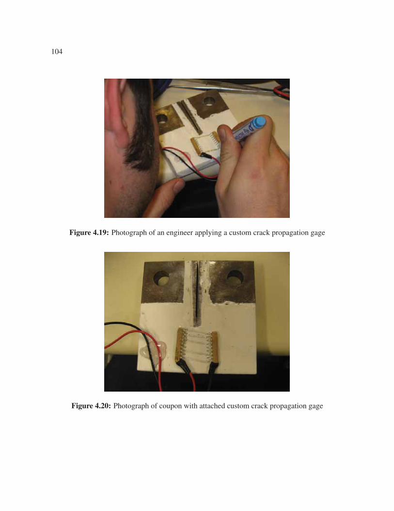
104
Figure 4.19: Photograph of an engineer applying a custom crack propagation gage
Figure 4.20: Photograph of coupon with attached custom crack propagation gage

105
The experimental procedure to test the custom crack propagation gage was also identical to
the one detailed in Section 4.2.2: The coupon was fatigued with no sensors or paint until the
crack propagation was initiated. Then, cyclic tension between 0.07 kip and 2.5 kip at 10 hertz
was applied to the specimen until failure.
4.3.4. Results and Discussion
After approximately one hour of fatigue testing, the crack propagated through the entirety of
the region covered by the custom crack gage. Figure 4.21 shows that all four painted rungs are
cleanly broken. Figure 4.22a shows a plot of the gage output versus time. Because this data
was taken with a wired data logger, it is more susceptible to the electromagnetic interference
generated by the test apparatus. Figure 4.22b shows the results of the application of a 0.1 hertz
low-pass Butterworth filter to the data. The data clearly show four distinct rung-breaks.
Figure 4.21: Coupon with custom gage after all rungs broken

106
1.6
1.8
2
2.2
2.4
2.6
2.8
3
0 500 1000 1500 2000 2500 3000 3500
Sens
or R
eadi
ng (V
)
Elapsed Seconds
Custom Crack Gage Output -- Unfiltered
(a)
1.6
1.8
2
2.2
2.4
2.6
2.8
3
0 500 1000 1500 2000 2500 3000 3500
Sens
or R
eadi
ng (V
)
Elapsed Seconds
Custom Crack Gage Output -- Low-Pass Filtered
(b)
Figure 4.22: Custom crack gage output versus time (a) unfiltered, and (b) with 0.1 hertz low-pass filter

107
4.4. Wireless ACPS Conclusions
This chapter has introduced Autonomous Crack Propagation Sensing (ACPS) and evalu-
ated two types of commercially available crack propagation gages and a newly invented crack
propagation gage for ACPS. It has also examined the potential of the Crossbow eKo Pro Series
Wireless Sensor Network for use in ACPS. The following conclusions can be drawn:
• The eKo Pro Series Wireless Sensor Network is suitable for use in ACPS provided care
is taken to accommodate its limited on-board analog-to-digital conversion hardware.
• Both types of the evaluated commercially available crack propagation pattern may be
used for ACPS, however, each has its disadvantages: The TK-09-CPA02-005/DP can
track crack tip position with a finer resolution, however, its non-linear output causes
the first 40-50% of its rung breaks to be undetectable by an eKo mote. The remaining
50-60% of its rung breaks, however, are easily detected. The TK-09-CPC03-003/DP,
conversely, is a larger gage with coarser resolution for crack to position. This gage’s
linear output characteristics enable each of its individual rung breaks to be detected by
the eKo mote.
• When applied to bare steel using the manufacturer-specified elevated-temperature-
cured adhesive, both types of traditional crack propagation patterns are capable of
functioning as ACPS sensors using eKo motes. When applied with a more field-
practical room-temperature-cured adhesive, the adhesive has been shown to fail before
the gage can break. These gages are therefore only usable in field conditions where
elevated-temperature-curing adhesive can be employed.
• Customized crack propagation gages made from conductive ink and commercially
available bus resistor networks can track crack propagation and conform to the eKo

108
motes’ strict analog specifications. These gages can be applied at room temperature
without adversely affecting sensor functionality. Customized crack propagation gages
allow for a single gage to track the propagation of a crack whose direction of propaga-
tion might be unknown or difficult to characterize.

109
CHAPTER 5
Conclusion
5.1. Conclusion
The preceding chapters have described the fundamentals of two wireless systems of au-
tonomous monitoring of cracks: Autonomous Crack Monitoring (ACM) and Autonomous Crack
Propagation Sensing (ACPS). ACM systems correlate the changes in the widths of cosmetic
cracks in residential structures with nearby vibration and with environmental effects to deter-
mine causal relationships. ACPS systems use crack propagation sensors affixed to steel bridge
members to track the propagation of existing cracks, alerting stakeholders to any growth. Wired
versions of these systems are expensive to install and intrusive to the users of the structures they
monitor. As wireless sensor networks (WSNs) decrease in size and cost and increase in capa-
bility and longevity, migrating ACM and ACPS systems from the wired to the wireless domain
will drastically decrease the time and cost of system installation as well as the disruption to the
users of instrumented structures. Chapter 2 described the sensors and components that make up
ACM and ACPS systems.
Chapter 3 described the challenges associated with moving an ACM system from the wired
to the wireless domain: sensor optimization, minimization of power consumption, and dynamic
event detection. Chapter 3 introduced the commercially available MICA2 WSN platform and
described three versions of a wireless ACM system built upon it, each with its own test deploy-
ment case study.

110
The three test deployments in Chapter 3 showed that with the proper power and network
management software components, the MICA2-based wireless ACM system is well-suited to
Mode 1 recording (periodic, single-point measurements taken from all sensors in a structure)
over a period of six to twelve months before a battery change is necessary. The test deploy-
ments showed that with the invention of the Shake ’n Wake hardware expansion board for the
MICA2 WSN platform, Mode 2 recording (high-frequency recording whenever an event of in-
terest is detected) can be partially implemented without sacrificing battery longevity. Though
Shake ’n Wake made possible low-power event detection, limitations in the existing software
drivers for the data acquisition board in the MICA2-based system prohibited triggered, high-
frequency sampling of all sensors.
Chapter 4 introduced the eKo Pro Series WSN, a commercially available product designed
for the agriculture industry but with capabilities that lend themselves well to ACPS: five-month
battery lifetime, integrated solar panels to extend the battery lifetime to five years, a simple
web-based interface that requires no programming by the user, and rugged outdoor-rated hous-
ing. Though no sensors have been manufactured to allow the eKo system to perform ACPS
monitoring, its implementation of the Environmental Sensor Bus (ESB) allows a third party
sensor manufacturer can create a custom interface such that a non-eKo sensor may be used with
any eKo mote.
Chapter 4 described two types of crack propagation sensors that were made compatible with
the ESB and made to function with the eKo motes. The first type, commercially manufactured
resistive crack patterns, are designed to be glued directly to steel in which a crack has formed.
The second type, a custom crack propagation gage, is designed to be drawn on to a painted
section of steel in which a crack has formed.

111
Chapter 4 described a series of experiments in which both types of commercially available
sensors were integrated with ESB circuitry and attached to steel compact tension specimens.
The pre-manufactured test coupons were functional and performed as designed when affixed
to the coupons using elevated temperature curing adhesive, but the first several rung-breaks of
the narrow gage were not recorded by the eKo mote due to their small voltage changes. The
gages attached to the coupon with room temperature curing adhesive were also functional but
prematurely de-bonded from the steel and ceased to function as the experiment progressed. Two
custom gages were drawn on a painted coupon at room temperature and performed as designed.
Since elevated temperature curing conditions are difficult to achieve on an in-service high-
way bridge, and since the propagation direction of a crack, and therefore the proper orientation
in which to install a pre-manufactured gage, may not be known at the time of installation, the
paint-on gage is more practical for field use than either of the pre-manufactured gages.
5.2. Future Work
5.2.1. Wireless Autonomous Crack Monitoring
Autonomous Crack Monitoring will continue to be a useful technique in litigation and regula-
tion of the mining and construction industries; reductions in cost, installation time, and intru-
siveness, made possible by implementing ACM using a WSN, will only make the technique
more useful. The MICA2 platform is now several years old and is not a focus of active hard-
ware development, therefore future wireless ACM work should be implemented on a different
WSN platform, such as the Microstrain V-Link, the Crossbow Imote, or the Moteware Irene
platforms. The Shake ’n Wake design can be modified to work with any WSN platform that
allows for direct physical and software access to the processor’s interrupt lines.

112
5.2.2. Wireless Autonomous Crack Propagation Sensing
Autonomous Crack Propagation Sensing has been proven in the lab and now must be qualified in
the field. The custom crack propagation patterns must be tested for overall field durability over
long periods of time. Additional experiments may be necessary to determine the best method
of physical protection of the circuitry and the painted traces of the custom crack propagation
gage.

113
References
Baillot, R. (2004). Crack response of a historic structure to weather effects and constructionvibrations. Master’s thesis, Northwestern University, Evanston, Illinois.
Bourns, I. (2006). 4600X Series - Thick Film Conformal SIPs.
Crossbow Technology, Inc. (2007a). MDA300CA Data Acquisition Board.http://www.xbow.com/Products/Product pdf files/Wireless pdf/MDA300CA Datasheet.pdf.
Crossbow Technology, Inc. (2007b). MPR-MIB Users Manual. http://www.xbow.com/Support/Support pdf files/MPR-MIB Series Users Manual.pdf.
Crossbow Technology, Inc. (2007c). MTS/MDA Sensor Board Users Manual. http://www.xbow.com/Support/Support pdf files/MTS-MDA Series Users Manual.pdf.
Crossbow Technology, Inc. (2007d). Stargate Gateway. http://www.xbow.com/Products/Product pdf files/Wireless pdf/Stargate Datasheet.pdf.
Crossbow Technology, Inc. (2007e). XMesh Users Manual. http://www.xbow.com/Support/Support pdf files/XMesh Users Manual.pdf.
Crossbow Technology, Inc. (2009a). eko pro series data sheet. http://www.xbow.com/eko/pdf/eKo pro series Datasheet.pdf.
Crossbow Technology, Inc. (2009b). eko pro series users manual. http://www.xbow.com/eko/pdf/eKo Pro Series Users Manual.pdf.
Crossbow Technology, Inc. (2009c). ESB developer’s guide.
Crossbow Technology, Inc. (2009d). MIB 510 Serial Interface Board. http://www.xbow.com/Products/Product pdf files/Wireless pdf/MIB510CA Datasheet.pdf.

114
Crossbow Technology, Inc. (2009e). MICA2 Wireless Measurement System.http://www.xbow.com/Products/Product pdf files/Wireless pdf/MICA2 Datasheet.pdf.
Dowding, C. H. (1996). Construction Vibrations. Prentice Hall, Upper Saddle River, NewJersey.
Dowding, C. H., Kotowsky, M. P., and Ozer, H. (2007). Multi-hop wireless system crackmeasurement for control of blasting vibrations. In Proc. 7th Int’l Symposium on Field Mea-surements in Geomechanics, Boston, Massachusetts. American Society of Civil Engineers.
Energizer Holdings, I. (2010a). Product datasheet: Energizer e91. http://data.energizer.com/PDFs/E91.pdf.
Energizer Holdings, I. (2010b). Product datasheet: Energizer l91. http://data.energizer.com/PDFs/l91.pdf.
Firstmark Controls (2010). Data sheet - series 150 subminiature position transducer. http://www.firstmarkcontrols.com/s021f.htm.
for Testing, A. S. and Materials (2006). Standard Test Method for Determination of Resistanceto Stable Crack Extension under Low-Constraint Conditions. ASTM E2472.
Geo Space Corporation (1980). GEO GS-14-L3 28 HZ 570 OHM. Part number 41065.
Geo Space Corporation (1996). HS-1-LT 4.5Hz 1250 Ohm Horiz. Part number 98449.
Hopwood, T. (2008). Personal communication with University of Kentucky researcher.
Hopwood, T. and Prine, D. (1987). Acoustic emission monitoring of in-service bridges. Tech-nical Report UKTRP-87-22, Kentucky Transportation Research Program, University of Ken-tucky, Lexington, Kentucky.
ITW CHEMTRONICS (2009). CircuitWoprks Conductive Pen TDS Num. CW2200.
Jevtic, S., Kotowsky, M. P., Dick, R. P., Dinda, P. A., and Dowding, C. H. (2007a). Luciddreaming: Reliable analog event detection for energey-constrained applications. In Proc.IPSN-SPOTS 2007, Cambridge, Massachusetts. Association for Computing Machinery / In-stitute of Electrical and Electronics Engineers.
Jevtic, S., Kotowsky, M. P., Dick, R. P., Dinda, P. A., Dowding, C. H., and Mattenson, M. J.(2007b). Lucid dreaming: Reliable analog event detection for energey-constrained applica-tions. Poster presented during live demonstration.

115
Kaman Measuring Systems (2009). Sensor data sheet: SMU-9000. http://www.kamansensors.com/html/products/pdf/wSMU9000-9200.pdf.
Kosnik, D. E. (2007). Internet-enabled geotechnical data exchange. In Proc. 7th Int’l Sympo-sium on Field Measurements in Geomechanics, Boston, Massachusetts. American Society ofCivil Engineers.
Kotowsky, M. P. (2010). Wireless sensor networks for monitoring cracks in structures: Sourcecode and configuration files. Addendum to MS Thesis.
Kotowsky, M. P., Dowding, C. H., and Fuller, J. K. (2009). Poster summary: Wireless sensornetworks to monitor crack growth on bridges. In Proceedings, Developing a Research Agendafor Transportation Infrastructure Preservation and Renewal Conference, Washington, DC.Transportation Research Board.
Louis, M. (2000). Autonomous Crack Comparometer Phase II. Master’s thesis, NorthwesternUniversity, Evanston, Illinois.
Macro Sensors (2009). Macro sensors LVDTs: DC-750 series general purpose DC-LVDTposition sensors. http://www.macrosensors.com/lvdt macro sensors/lvdt products/lvdt position sensors/dc lvdt/free core dc/dc 750 general purpose.html.
Marron, D. R. (2010). Personal communication with Chief Research Engineer at the Infrastruc-ture Technology Institute at Northwestern University.
Maxim Integrated Products (2003). SOT23, Dual, Precision, 1.8V, Nanopower ComparatorsWith/Without Reference. Part number MAX9020EKA-T.
Maxim Integrated Products, Inc. (2009). 1024-bit, 1-wire eeprom data sheet.
McKenna, L. M. (2002). Comparison of measured crack response in diverse structures to dy-namic events and weather phenomena. Master’s thesis, Northwestern University, Evanston,Illinois.
Moxa, Inc (2010). UC-7410/7420 Series. http://www.moxa.com/doc/specs/UC-7410 7420 Series.pdf.
Ozer, H. (2005). Wireless sensor networks for crack displacement measurement. Master’sthesis, Northwestern University, Evanston, Illinois.
Puccio, M. (2010). Personal communication with Application Engineer of Macro Sensors.

116
Siebert, D. (2000). Autonomous Crack Comparometer. Master’s thesis, Northwestern Univer-sity, Evanston, Illinois.
Snider, M. (2003). Crack response to weather effects, blasting, and construction vibrations.Master’s thesis, Northwestern University, Evanston, Illinois.
SOLA HD (2009). SCL Series, 4 and 10 Watt CE Linears. http://www.solahd.com/products/powersupplies/pdfs/SCL.pdf.
SoMat, Inc. (2010). eDAQ Simultaneous High Level Layer. http://www.somat.com/products/edaq/edaq simultaneous high level layer.html#tabs-1-2.
Speckman, G. M. (2010). Personal communication with Regional Sales Manager of KamanSensors.
Stolze, F., J.Staszewski, W., Manson, G., and Worden, K. (2009). Fatigue crack detectionin a multi-riveted strap joint aluminium panel. In Kundu, T., editor, Health monitoring ofstructural and biological systems, volume 7925. Bellingham, Wash. : SPIE.
Switchcraft Inc. (2004). EN3™Cord Connector.
The Sherwin-Williams Company (2019). MACROPOXY 646 FAST CURE EPOXY.
United States Department of Transportation: Federal Highway Administration (2006). BridgeInspector’s Reference Manual, volume 2. National Highway Institute.
Vishay Intertechnology, Inc. (2008). Special use sensors - crack propagation sensors.
Waldron, M. (2006). Residential crack response to vibrations from underground mining. Mas-ter’s thesis, Northwestern University, Evanston, Illinois.

117
APPENDIX A
Experimental Verification of Shake ’n Wake
This appendix describes experiments detailing experimental verification of the design criteria
of the Shake ’n Wake board.

118
The design criteria of the Shake ’n Wake board are as follows:
(1) It must not significantly increase the power consumption of a mote.
(2) Its trigger threshold must be predictable and repeatable.
(3) It must not contaminate the output signal of its attached sensor.
(4) It must wake up the mote such that the mote has time to record during the peak of the
motion of interest.
Criterion 1 is addressed in Section 3.3.7.3. Verification of the rest of the design critera are
described in the following sections.
A.1. Transparency
Because Shake ’n Wake is intended to be attached in parallel an analog-to-digital conver-
sion unit on the mote, the output of the geophone must not be affected by the presence of the
Shake ’n Wake. To determine whether the Shake ’n Wake hardware meets this design criterion,
the output of the test geophones attached to Shake ’n Wake boards were compared to control
geophones while subjected to identical physical excitation. Figure A.1 shows the experimen-
tal setup on which all four geophones – an HS-1 test geophone, an HS-1 control geophone, a
GS-14 test geophone, and a GS-14 control geophone, were placed on the end of a cantilevered
aluminum springboard at an identical distance from the fulcrum.
By measuring the responses of the geophones connected to Shake ’n Wake boards and com-
paring them to the responses of the control geophones, it can be determined whether or not
the Shake ’n Wake circuitry will contaminate the waveform. Figure A.2 clearly indicates that
the positive portion of the output of a test geophone follows the positive portion of the output
of its equivalent control geophone. The negative portion of the output of the test geophone is

119
Figure A.1: Shake ’n Wake transparency test apparatus
clipped at a value of -200 millivolts. The negative portion of the output of a geophone attached
to a Shake ’n Wake is clipped by reverse-current-limiting diodes that prevent voltage of inap-
propriate polarity from damaging the board’s internal electronics. When the same geophone is
attached to the opposite connector on the Shake ’n Wake, similar clipping of the positive por-
tion of the waveform can be observed. These results show that the Shake ’n Wake satisfies the
requirement of not corrupting the output of the geophone.
A.2. Verification of Trigger Threshold
Idealized analysis of the Shake ’n Wake’s adjustable trigger circuit, pictured in Figure 3.24,
indicates that for any trigger setting, x, the threshold, Vcomp at which the Shake ’n Wake will
bring the mote out of its low-power sleep state is 3.558mV ∗ x. To verify the validity of this
idealized analysis, the output of an HS-1 geophone is recorded on the same time scale as the
output of the Shake ’n Wake to which it is attached, and the output of a GS-14 geophone is

120
-1000
-500
0
500
1000
1500
2000
46 46.5 47 47.5 48 48.5 49 49.5 50
Inpu
t sin
gal (
mV)
Time (seconds)
S ’n W vs. Control (HS-1)
Control geophoneGeophone attached to S’nW
Figure A.2: Shake ’n Wake transparency test results for HS-1 geophone
recorded on the same time scale as the output of the Shake ’n Wake to which it is attached.
Both geophones were placed on a cantilevered aluminum springboard with identical distances
from the fulcrum. Figure A.3 shows this experimental setup.
The length of the springboard was decreased successively to produce response frequencies
of 5, 10, 15, and 20 hertz, thereby spanning the frequency range of interest for structural motion
in response to a vibration event. The Shake ’n Wake was set to level 2 of 31, the most sensitive
level that could be used while avoiding false triggers from ambient vibration of the springboard.
Figures A.4 and A.5 show the voltage level at which each Shake ’n Wake triggers with a
threshold setting of level 2 when the geophones are moved at a frequency of 5 hertz.

121
Figure A.3: Shake ’n Wake trigger threshold test apparatus
Figure A.4: Shake ’n Wake Level 2 trigger threshold test results for HS-1 geophone at 5 hertz
For each of the set of test frequencies, averages of the voltage level at which the Shake ’n Wake
triggered were computed. Figure A.6 graphically summarizes these results. Based on the anal-
ysis of the idealized trigger threshold reference circuit in Figure 3.24, the theoretical value at
which the Shake ’n Wake should trigger – regardless of the sensor to which it is attached – is
7.116 millivolts. Figure A.6 indicates that the Shake ’n Wake is actually triggered at a higher

122
Figure A.5: Shake ’n Wake Level 2 trigger threshold test results for GS-14 geophone at 5 hertz
voltage threshold than predicted, and the actual trigger threshold varies with frequency of the
output of the geophone.
These results indicate that the idealized analysis is not adequate to determine the actual volt-
age threshold at which the Shake ’n Wake will trigger; frequency also must be taken into account
when determining this voltage. The dependence of the Shake ’n Wake’s comparators on the fre-
quency of their input voltage can be attributed to the hysteresis of the comparator, described in
detail in the comparator’s product data sheet in Maxim Integrated Products (2003). In order to
accurately determine the threshold voltage, the Shake ’n Wake must be calibrated by the user
with the desired sensor over the range of desired input frequencies. Though Figures A.4 and A.5
do indicate that though the trigger threshold varies with frequency, it is predictable; in each pe-
riod of the input waveform, the trigger occurs at approximately the same input voltage. This

123
satisfies the requirement that the trigger threshold be both predictable and repeatable, though
sensor- and frequency-specific calibration is required for precise predictions.
6
8
10
12
14
16
18
20
5 10 15 20
aver
age
outp
ut a
t whi
ch s
yste
m tr
igge
rs (m
illiv
olts
)
motion frequency (Hz)
Trigger threshold vs. motion frequency
GS-14 Geophone (measured)
HS-1 Geophone (measured)
Theoretical Trigger Level
Figure A.6: Summary of Shake ’n Wake level 2 trigger threshold voltages
A.2.1. Physical Meaning of Trigger Threshold
The HS-1 and the GS-14 geophones each have a different characteristic response to vibration
phenomena. These responses are shown graphically in Appendices B.8 and B.9, respectively.
Figure A.7 shows the trigger levels derived from the springboard experiment translated into
terms of particle velocity. Over the frequency range of interest, the response of an undamped
HS-1 geophone can be determined using the factory calibration sheet included in Appendix B.9.
The GS-14 geophone, however, is not typically used for detection of low-frequency motion, so

124
the relationship between its voltage and frequency has not been included in the factory calibra-
tion curve in Appendix B.8. Its low-frequency response can be extrapolated from the factory-
provided curve using a power law formula as follows:
The cantilever vibration displacement δ can be held constant during the experiment by ap-
plying identical tip displacement. Its velocity is then equal to 2πfδ. Even with a constant δ,
the velocity increases linearly for the portion of the GS-14’s response curve where frequency is
less than 20 hertz. Therefore, the portion of the GS-14’s response curve can be described with
the following power law formula:
v = 2πδkfn
where f is the frequency of motion, k is a constant that depends on the damping of the geophone,
n is the slope of the response curve on a logarithmic plot, and v is the voltage per inch per
second of geophone output at frequency f . For the undamped response curve (A), used in this
experiment to provide the largest signal-to-noise ratio to the Shake ’n Wake board, this portion
of the response curve can be approximated as:
v = 2.455 ∗ 10−5 ∗ f 3.106
A.3. Speed
The Shake ’n Wake board does not have the ability to digitally record the readings from
the sensor to which it is attached. It is therefore crucial to the operation of a system perform-
ing Mode 2 recording that the mote to which the Shake ’n Wake is attached begins to operate
and execute user code as quickly as possible, as it will be the user code that is responsible for

125
0.002
0.004
0.006
0.008
0.01
0.012
0.014
0.016
5 10 15 20
velo
city
at w
hich
S ’n
W tr
igge
rs (i
n/se
c)
motion frequency (Hz)
Trigger threshold vs. motion frequency (HS-1)
measured
theoretical
0
0.1
0.2
0.3
0.4
0.5
5 10 15 20
velo
city
at w
hich
S ’n
W tr
igge
rs (i
n/se
c)
motion frequency (Hz)
Trigger threshold vs. motion frequency (GS-14)
= 3.069 ips
= 1.955 ips
measured
theoretical
Figure A.7: Summary of Shake ’n Wake level 2 trigger threshold velocities
recording the event. If a wireless ACM system were deployed to measure dynamic response
of a residential structure, the highest frequency input signal to which the Shake ’n Wake must
respond is 20 hertz; this is the highest expected frequency of motion of an instrumented wall.

126
Figure A.8 shows that a 20 hertz zero-centered sinusoidal input signal will reach its peak abso-
lute amplitude after 12.5 milliseconds.
0 0.0125 0.025 0.0375 0.05
Sing
al a
mpl
itude
Time (sec)
period = 0.05
first peak at quarter of the period
Figure A.8: 20 hertz sinusoidal input signal with rise time of 12.5 milliseconds
If it is assumed that the mote must be awake for at least one full sample length before the
peak of interest and that it will be sampling at 1000 hertz, then it follows that the time from
Shake ’n Wake event detection to the execution of user code by the mote must be less than 11.5
milliseconds.
Output from an oscilloscope connected to various components of a wireless ACM node,
shown in Figure A.9, illustrates signal propagation delay from the geophone through the com-
ponents of the Shake ’n Wake and finally into the mote’s processor. At time t1 = 60μs, the out-
put voltage of the geophone, shown in yellow, crosses the threshold V1 which corresponds to the
software programmable threshold residing in the Shake ’n Wake’s memory. 58μs later, at time
t2, the Shake ’n Wake’s hardware interrupt request line (IRQ), shown in green, changes to logic
low. This change in state of the IRQ is the “wakeup” signal passing from the Shake ’n Wake to

127
the mote. The mote, which is asleep until t2, has already been programmed by the user with an
instruction to turn on an LED. The LED active-low hardware line, shown in purple, activates at
t3, 31μs after the signal from the Shake ’n Wake is sent to the mote. The activation of the LED
indicates that the mote has executed its first line of user code. In a real event detection system,
this first post-wakeup instruction would be to immediately begin sampling at a high frequency.
The power draw of entire system, shown in pink, begins to increase from its sleep level as soon
as the Shake ’n Wake sends its “wakeup” signal.
This timing diagram shows that the interval between the moment the input signal reaches
the theoretical trigger threshold and the moment the Shake ’n Wake signals a “wakeup” is 58 μs
and the time interval between when the Shake ’n Wake signals a “wakeup” and the time the
first line of user code is executed on the mote is 31 μs. Since this 89 μs is well within the
specified 11.5 millisecond window, it follows that the Shake ’n Wake can perform within the
timing requirements.
A.4. Discussion
These experiments have served to quantify the abilities of the Shake ’n Wake hardware rela-
tive to the requirements of a random-event detection scenario. The suitability of the geophones
is limited on one end by amplitude: if the vibration frequency is not high enough, the required
output amplitude for the Shake ’n Wake to trigger at its most sensitive setting becomes unreach-
able. On the other end of the frequency range, the limit of functionality is the response speed of
the Shake ’n Wake hardware. Table A.1 summarizes the practical limits of the Shake ’n Wake
with respect to frequency of geophone output.

128
Geophone: 50mV/div
IRQ: 4 V/div
LED: 4 V/div
Current: 5 mA/div
V1
t1 t2 t3t2 - t1 = 58.0ms t3 - t2 = 31.0ms20ms
Figure A.9: Scope readout indicating the mote can execute user code within 89 μs of a signalof interest, after Jevtic et al. (2007b)
A.4.1. Upper Frequency Limit: Shake ’n Wake Response Time
A mote attached to a Shake ’n Wake will be executing user code 89 μs after a geophone voltage
of interest. Using the same assumption that the mote must be awake for at least one full sample
period before the peak of interest and that it will be sampling at 1000 hertz once it wakes up,
the minimum time between the “wakeup” signal and the arrival of the peak of the event is 1.089
milliseconds. Figure A.8 indicates that the rise time of an idealized sinusoidal input signal is
25% of its period. If the rise time must be at least 1.031 milliseconds, then the period must be
at lest 4.356 milliseconds and the frequency must be at most 230 hertz. Thus, in order for a
node to be executing user code in time to catch the first peak of a dynamic event of interest, the
maximum frequency of the event is 230 hertz.

129
A.4.2. Lower Frequency Limit: Geophone Output Amplitude
The GS-14 and HS-1 geophones’ output amplitude for a given input velocity varies with fre-
quency, as shown in the response spectra in Appendices B.8 and B.9, respectively. Figure A.7
shows that for the GS-14 geophone, the frequency of motion must be greater than 20 hertz be-
fore a 0.05 inch per second velocity can be detected by the Shake ’n Wake at level 2. However,
if the amplitude of motion is great enough, the GS-14 can produce sufficient amplitude at low
frequencies. For the HS-1 geophone, the frequency of motion can be as low as 2 hertz and still
provide a large enough amplitude to trigger the Shake ’n Wake at level 2, no matter what the
amplitude of the motion.
input velocity > 1ips 0.05ips
GS-14 2 − 230Hz 20 − 230Hz
HS-1 2 − 230Hz 2 − 230Hz
Table A.1: Summary of functional ranges for Shake ’n Wake event detection at level 2
A.5. Appendix Conclusion
The above experiments verify that the Shake ’n Wake:
• does not contaminate the sensor output
• provides a predictable and repeatable threshold voltage
• responds quickly enough to allow the mote to wake up in time to digitally record the
signal of interest

130
– can be used with a GS-14 geophone to detect motions with a frequency 20 hertz
and 230 hertz at amplitudes of 0.05 ips, down to 2 hertz if amplitude is sufficiently
large
– can be used with an HS-1 geophone to detect motions with a frequency between
2 hertz and 230 hertz regardless of amplitude

131
APPENDIX B
Data Sheets and Specifications
The following pages contain specification and data sheets for all relevant commercially manu-
factured equipment described in this thesis. All documents are reproduced in their entirety as
they existed on the Web at the time of publication of this document and without any modifica-
tion.

132
B.1. MICA2 Data Sheet
P h o n e : 4 0 8 . 9 6 5 . 3 3 0 0 F a x : 4 0 8 . 3 2 4 . 4 8 4 0 E - m a i l : i n f o @ x b o w . c o m W e b : w w w . x b o w . c o m
WIRELESS MEASUREMENT SYSTEM
MICA2
MICA2 The MICA2 Mote is a third genera-tion mote module used for enabling low-power, wireless, sensor networks. The MICA2 Mote features several new improvements over the original MICA Mote. The following features make the MICA2 better suited to commercial de-ployment:
• 868/916 MHz multi-channel transceiver with extended range
• Supported by MoteWorks™ wireless sensor network platform for reliable, ad-hoc mesh networking
• Support for wireless remote reprogramming
• Wide range of sensor boards and data acquisition add-on boards
MoteWorks enables the development of custom sensor applications and is specifically optimized for low-power, battery-operated networks. MoteWorks is based on the open-source TinyOS operating system and provides reliable, ad-hoc mesh networking, over-the-air-programming capabilities, cross development tools, server middleware for enterprise network integration and client user interface for analysis and configuration.
Processor and Radio Platform (MPR400)The MPR400 is based on the Atmel ATmega128L. The ATmega128L is a low-power microcontroller which runs MoteWorks from its internal flash memory. A single processor board (MPR400) can be configured to run your sensor application/pro-cessing and the network/radio communications stack simultane-ously. The MICA2 51-pin expansion connector supports Analog Inputs, Digital I/O, I2C, SPI and UART inter-faces. These interfaces make it easy to connect to a wide variety of exter-nal peripherals.
Sensor BoardsCrossbow offers a variety of sensor and data acquisition boards for the MICA2 Mote. All of these boards con-nect to the MICA2 via the standard 51-pin expansion connector. Custom sensor and data acquisition boards are also available. Please contact Cross-bow for additional information.
• 3rd Generation, Tiny, Wireless Platform for Smart Sensors
• Designed Specifically for Deeply Embedded Sensor Networks
• > 1 Year Battery Life on AA Batteries (Using Sleep Modes)
• Wireless Communications with Every Node as Router Capability
• 868/916 MHz Multi-Channel Radio Transceiver
• Expansion Connector for Light, Temperature, RH, Barometric Pressure, Acceleration/Seismic, Acoustic, Magnetic and other Crossbow Sensor Boards
Applications• Wireless Sensor Networks
• Security, Surveillance and Force Protection
• Environmental Monitoring
• Large Scale Wireless Networks (1000+ points)
• Distributed Computing Platform
Antenna
Logger Flash
ProcessorAnalog I/ODigital I/O
Tunable FrequencyRadio
51-Pin Expansion Connector
MMCXConnector
Document Part Number: 6020-0042-08 Rev A
MPR400 Block Diagram

133
C r o s s b o w Te c h n o l o g y , I n c . 4 1 4 5 N o r t h F i r s t S t r e e t S a n J o s e , C a l i f o r n i a 9 5 1 3 4 - 2 1 0 9
Base StationsA base station allows the aggregation of sensor network data onto a PC or other computer platform. Any MICA2 Mote can function as a base station when it is connected to a standard PC interface or gateway board. The MIB510/MIB520 provides a serial/USB interface for both programming and data communications. Crossbow also offers a stand-alone gateway solution, the MIB600 for TCP/IP-based Ethernet networks.
Document Part Number: 6020-0042-08 Rev A
Notes: Specifications subject to change without notice
Processor/Radio Board MPR400CB Remarks
Processor Performance
Program Flash Memory 128K bytes
Measurement (Serial) Flash 512K bytes >100,000 Measurements
Configuration EEPROM 4K bytes
Serial Communications UART 0-3V transmission levels
Analog to Digital Converter 10 bit ADC 8 channel, 0-3V input
Other Interfaces DIO,I2C,SPI
Current Draw 8 mA Active mode
< 15 μA Sleep mode
Multi-Channel Radio
Center Frequency 868/916 MHz ISM bands
Number of Channels 4/ 50 Programmable, country specific
Data Rate 38.4 Kbaud Manchester encoded
RF Power -20 to +5 dBm Programmable, typical
Receive Sensitivty -98 dBm Typical, analog RSSI at AD Ch. 0
Outdoor Range 500 ft 1/4 Wave dipole, line of sight
Current Draw 27 mA Transmit with maximum power
10 mA Receive
< 1 μA Sleep
Electromechanical
Battery 2X AA batteries Attached pack
External Power 2.7 - 3.3 V Connector provided
User Interface 3 LEDs User programmable
Size (in) 2.25 x 1.25 x 0.25 Excluding battery pack
(mm) 58 x 32 x 7 Excluding battery pack
Weight (oz) 0.7 Excluding batteries
(grams) 18 Excluding batteries
Expansion Connector 51-pin All major I/O signals
Ordering Information
Model Description
WSN-START900CA MICA2 Starter Kit 868/916 MHz
WSN-PRO900CA MICA2 Professional Kit 868/916 MHz
MPR400CB 868/916 MHz Processor/Radio Board
MIB520 Mote Interface Board

134
B.2. String Potentiometer Data Sheet
Providing the Ultimate Solutions inPrecision Displacement Sensors
Order � Site Map
Home All Products Support Special Offers Contact Us
Home
Data Sheet - Series 150 Subminiature Position Transducer
World's Smallest Cable Position Transducer
Shaded characteristics are verified during production and test. All others are for REFERENCE and informationonly.
Key Features
1.5-Inch (38-mm) Maximum Travel1.Analog Signal Using Precision Conductive Plastic Potentiometer2.AccuTrakTMGrooved Drum for Enhanced Repeatability3.Small, Robust Design4.Choice of Displacement Cable Pull Direction5.DirectConnectTM Sensor-To-Drum Technology = Zero Backlash,No Torsion Springs or Clutches
6.
Potentiometer Specifications
Potentiometer Type 1-turn, precision, conductive plasticResistance: Value, Tolerance 5K ohms, ±10%Travel: Electrical, Mechanical 340°, 340° min
nim snoitulover tfahs noillim 5efiL lacinahceM)tiucric redivid egatlov( egatlov ylppus ot 0 morf langis golanalangiS tuptuO
)C °07( F °851 ta W 57.0gnitaR rewoPxam Am 21tnerruC ylppuS
)tiucric redivid egatlov gnisu( xam CDV 53egatloV ylppuSIndependent Linearity Error ±1.0% max per VRCI-P-100AOutput Smoothness 0.1% maxInsulation Resistance 1000 Mohms at 500 VDC min
nim CDV 005htgnertS cirtceleiDlangis etinifninoituloseR
Operating Temperature -85° to +257° F (-65° to +125° C)32093-R-liM rep g 51 ta zH 0002 ot 01 ,sm 6 rof g 001noitarbiV ,kcohS
Temperature Coefficient ±400 ppm/°C max
Other Specifications
th.f120s/moc.slortnockramtsrif.www//:ptthrecudsnarT noitisoP erutainimbuS 051 seireS - teehS ataD m
1 of 3

135
munimula 4202 dezidona denihcam-noisicerpslairetaM esaC
Displacement Cable 0.018-inch (0.46-mm) dia., 7-by-7 stranded stainless steel, 40-lb (177-N)min breaking strength
DisplacementCable Hardware
1 each of 300196 loop sleeve, 300292 copper sleeve, 300688 ball-end plug,300495 pull ring, 160026 brass swivel, and 301003 nickel swivel; all itemsprovided uncrimped
)g 0.51( zo 5.0ssaM lanimoN
Displacement Cable Tension and CableAcceleration (Nominal): Opt. 1
1 oz 0.3 N min6 oz 1.7 N max 29 g max
Displacement Cable Tension and CableAcceleration (Nominal): Opt. 2
3 oz 0.8 N min14 oz 3.9 N max 49 g max
Environmental Protection NEMA 3S / IP 54; DO-160D (ED-14D) Env. Cat.E1E1ABXHXFDXSAXXXXXXXXXX
Model Numbers and Ordering Codes
)egnar )mm-83( hcni-05.1( recudsnart noitisopcba-1210-051Example: 150-0121-L2N (left-hand displacement cable pull, cable tension: -020, no base)
Variable Value Description
aL left-hand displacement cable pullR right-hand displacement cable pull
b1 cable tension: -0102 cable tension: -020
cN no baseB base: L; pn 150015
Drawing
th.f120s/moc.slortnockramtsrif.www//:ptthrecudsnarT noitisoP erutainimbuS 051 seireS - teehS ataD m
2 of 3

136
Electrical Connection for Increasing Output with Displacement Cable ExtractionLeft-Hand Pull
blackwhitered
Right-Hand Pullred
whiteblack
Signalinput, V+
output, signal, S+ground, common, V-, S-
For crimping of hardware to displacement cable, consider the 160001-01 installation kit.
Need something not shown? Complete a Custom Solution Request.
All dimensions are REFERENCE and are in inches [mm] � Data Sheet Series 150 Rev. -
Privacy PolicyPrivacy Policy
Firstmark Controls � [email protected] ISO9001:2000/AS9100B-Compliant Company1176 Telecom Drive � Creedmoor, NC 27522 USAPhone: 1-919-956-4203 � Fax: 919-682-3786 � Toll Free:1-866-912-6232
Business hours: Mon-Fri, 8:00am to 5:00pm (Eastern time)All specifications subject to change without notice.
© 1996-2010 Firstmark Controls All rights reserved.
top Newsletter � -->News � Representatives � Request Literature � CAD Models � Calculators top
th.f120s/moc.slortnockramtsrif.www//:ptthrecudsnarT noitisoP erutainimbuS 051 seireS - teehS ataD m
3 of 3

137
B.3. MDA300CA Data Sheet
P h o n e : 4 0 8 . 9 6 5 . 3 3 0 0 F a x : 4 0 8 . 3 2 4 . 4 8 4 0 E - m a i l : i n f o @ x b o w . c o m W e b : w w w . x b o w . c o m
MDA300Developed at UCLA’s Center for Embedded Network Sensing (CENS), the MDA300 is an extremely versatile data acquisition board that also in-cludes an onboard temperature/ humidity sensor. With its multi-function direct user interface, the MDA300 of-fers a convenient and flexible solution to those sensor modalities commonly found in areas such as environmental and habitat monitoring as well as many other custom sensing applications.
As part of a standard mesh network of Motes, the MDA300’s easy access micro-terminals also make it an economical solution for a variety of ap-plications and a key component in the next generation of low-cost wireless weather stations. Data logging and display is supported via Crossbow’s MoteView user interface.
Crossbow’s MoteView software is designed to be the primary interface between a user and a deployed net-work of wireless sensors. MoteView provides an intuitive user interface to database management along with sensor data visualization and analysis tools. Sensor data can be logged to a database residing on a host PC, or to a database running autonomously on a Stargate gateway.
DATA ACQUISITION BOARD
MDA300
Document Part Number: 6020-0052-03 Rev A
Communication and Control Features Including:
• 7 single-ended or 3 differential ADC channels• 4 precise differential ADC channels• 6 digital I/O channels with event detection interrupt• 2.5, 3.3, 5V sensor excitation and low-power mode• 64K EEPROM for onboard sensor calibration data• 2 relay channels, one normally open and one normally closed• 200 Hz counter channel for wind speed, pulse frequencies• External I2C interface
Drivers for the MDA300 board are included in Crossbow’s MoteWorks™ software platform. MoteWorks enables the development of custom sensor applications and is specifically optimized for low-power, battery-operated networks. MoteWorks is based on the open-source TinyOS operating system and provides reliable, ad-hoc mesh networking, over-the-air-programming capabilities, cross development tools, server middleware for enterprise network integration and client user interface for analysis and configuration.
Ordering Information
• Multi-Function Data Acquisition Board with Temp, Humidity Sensor
• Compatible with MoteView Driver Support
• Up to 11 Channels of 12-bit Analog Input
• Onboard Sensor Excitation and High-Speed Counter
• Convenient Micro-Terminal Screw Connections
Applications• Environmental Data Collection
• Agricultural and Habitat Monitoring
• Viticulture and Nursery Management
• HVAC Instrumentation and Control
• General Data Collection and Logging
Model Description
MDA300CA Mote Data Acquistion Board with Temperature and Humidity
2.25"
1.8"
MDA300CA Data Acquisition Block Diagram
51 Pin Expansion Connector
Humidityand
TemperatureSensor
Co
un
ter
I2C B
us
EEPROM
8-Channel Digital I/O
4:1 MUX
Differential inputs
+ -
7 Single-Ended or 3 Differential
8-Channel 12-Bit A/D
RelayRelay
MDA300C Block Diagram

138
B.4. MIB510CA Data Sheet
P h o n e : 4 0 8 . 9 6 5 . 3 3 0 0 F a x : 4 0 8 . 3 2 4 . 4 8 4 0 E - m a i l : i n f o @ x b o w . c o m W e b : w w w . x b o w . c o m
MI B510The MIB510 allows for the aggrega-tion of sensor network data on a PC as well as other standard computer platforms. Any IRIS/MICAz/MICA2 node can function as a base station when mated to the MIB510 serial interface board. In addition to data transfer, the MIB510 also provides an RS-232 serial programming interface.
The MIB510 has an onboard processor that programs the Mote processor/radio boards. The proces-sor also monitors the MIB510 power voltage and disables programming if the voltage is not within the required limits. Two 51-pin Hirose connectors are available, allowing sensor boards to be attached for monitoring or code development. The MIB510 is also compatible with the Atmel JTAG pod for code development.
SpecificationsRS-232 Interface• Connector: 9-pin “D”
• Baud Rates: - User defined (57.6k typical) - Programming: 115.2k (uisp controlled)
SERIAL INTERFACE BOARD
M I B510
• Base Station for Wireless Sensor Networks
• Serial Port Programming for IRIS, MICAz and MICA2 Hardware Platforms
• Supports JTAG code debugging
Applications• Programming Interface
• RS-232 Serial Gateway
• IRIS, MICAz, MICA2 Connectivity
Document Part Number: 6020-0057-03 Rev A
Mote Interface
• Connectors: - 51 pin (2)
• Indicators: - Mote LEDs: Red,
Green, Yellow
Programming Interface
• Indicators: - LEDs - Power Ok (Green),
Programming in Progress (Red)
• Switches: - On/Off switch to disable the
Mote serial transmission - Temporary switch to reset the
programming processor and Mote
Jtag Interface• Connector: 10-pin male header (2)
Power• 5V @ 50mA using external power supply (included with unit)
• 3.3-2.7V @ 50mA using Mote batteries
Ordering Information
MIB510 with Mote and Sensor Board
Model Description
MIB510 Serial PC Interface Board
MIB510CA Block Diagram
ISP uP
MICA2/MICA2DOT
Sensor Board
Serial Port
MIB510 Block Diagram

139
B.5. Stargate Data Sheet
P h o n e : 4 0 8 . 9 6 5 . 3 3 0 0 F a x : 4 0 8 . 3 2 4 . 4 8 4 0 E - m a i l : i n f o @ x b o w . c o m W e b : w w w . x b o w . c o m
X-SCALE, PROCESSOR PLATFORM
STARGATE
• 400 MHz, Intel PXA255 Processor
• Low Power Consumption <500 mA
• Embedded Linux BSP Package, Source Code Shipped with Kit
• Small, 3.5” x 2.5” Form Factor
• PCMCIA and Compact Flash Connector
• 51-pin Expansion Connector for IRIS/MICAz/MICA2 Motes and other Peripherals
• Ethernet, Serial, JTAG, USB Connectors via 51-pin Daughter Card Interface
• Li-Ion Battery Option
Applications• Sensor Network Gateway
• Robotics Controller Card
• Distributed Computing Platform
Document Part Number: 6020-0049-05 Rev A
The Stargate processor module is compatible with Crossbow’s IRIS/MICAz/MICA2 family of wireless sensor networking products and the public domain software from Intel’s Open-Source Robotics initiative. The Stargate processor module is also an ideal solution for standalone Linux-based Single Board Computer (SBC) applications.
With its strong communications capability and Crossbow’s ongoing commitment to its open-source archi-tecture, the Stargate platform offers tremendous flexibility. The SPB400CB Processor Board has both Compact Flash and PCMCIA connectors as well as optional installable headers for 2 serial ports and an I2C port. The SDC400CA Daughter Card supports a variety of additional interfaces, including:
• RS-232 Serial • 10/100 Ethernet • USB Host • JTAG
Finally, the standard Mote connector on the SPB400CB Processor Board provides support for synchronous serial port (SSP), UART, and other GPIO connections.
STARGATEThe Stargate is a high-performance processing platform designed for sensor, signal processing, control and wireless sensor networking applica-tions and is based on Intel’s Xscale® processor.
The Stargate processor board is the result of the combined design efforts of several different Ubiquitous Com-puting research groups within Intel. The completed design is licensed to Crossbow Technology for commercial production. The Stargate processor board is preloaded with a Linux distri-bution and basic drivers. A variety of useful applications and development tools are also provided.
3.50"
2.49"
.020"
.020"
340"1.800"
1.355"
3.30"
.120"
2.135"
2.290"
.10".10"
Processor Board
2.00"
2.49"
1.800" .10"
2.290"
.10"
.020"
.020"
Daughter Card

140
C r o s s b o w Te c h n o l o g y , I n c . 4 1 4 5 N o r t h F i r s t S t r e e t S a n J o s e , C a l i f o r n i a 9 5 1 3 4 - 2 1 0 9
Document Part Number: 6020-0049-05 Rev A
Ordering Information
Specifications subject to change without notice
Stargate Kit Contents
Stargate Processor Board
Stargate Daughter Card
Power Supply
Null Modem Cable
CD-ROM
CD-ROM Contents
Linux - Kernel & Driver Sources
GNU Cross Platform Dev. Tools
Bootloader with Source Code
Flash Programming Utility
Shareware & Test Applications
Developer’s Guide - PDF Format
Model Description
SP-KIT400CA Stargate Developer’s Kit
SPB400CB Stargate Processor Board
SDC400CA Stargate Daughter Card - JTAG, 10/100 Ethernet, Serial, USB Host
Specifications Remarks
STARGATE Processor Board
Intel PXA255, Xscale® 400 MHz, RISC Processor
Intel SA1111, StrongARM® Multiple I/O Companion Chip
Memory
64 MB SDRAM
32 MB FLASH Linux Software < 10 MBytes
Communications
PCMCIA Slot Type II
Compact Flash Slot Type II
51-pin GPIO UART, SSP via Mote Connector
Optional I2C Port Installable Header
Optional Serial Port (2) Installable Header
General
Li-Ion Battery Option
Watch Dog Timer (WDT) Configurable up to 60 seconds
Battery Gas Gauge
LED and User Application Switch
Power Switch
STARGATE Daughter Card
Communications
10 Base-T Ethernet Port RJ-45 Connector
RS-232 Serial Port DB-9 Connector
JTAG Debug Port
USB Host Port Version 1.1
General
A/C Power Adaptor 5-6 VDC, 1 Amp
Reset Button
Real-Time Clock
Physical
Processor Board (in) 3.50 x 2.49 x 0.73
(cm) 9.53 x 6.33 x 1.86
Weight (oz) 1.68
(g) 47.47
Daughter Card (in) 2.49 x 2.00 x 0.60
(cm) 6.33 x 5.08 x 1.52
Weight (oz) 1.42
(g) 40.16
Environmental
Operating Temperature 0 to +70 (°C)
Processor Board - Top
MICA2/GPIO Connector
INTELPXA255
OptionalI2C
Connector
SDRAM 64 MB
INTELSA 1111
SerialController
Ethernet
RJ-45
JTAGConnector
Gas Gauge
WatchDog Timer
LED
USBHost Port
Compact Flash
PCMCIA
Flash32 MB
LANController
OptionalSerial
Connector
RS-232
Daughter Card
Processor Board
Daughter Card
Stargate Block Diagram

141
B.6. Alkaline Battery Data Sheet
AA
Classification: AlkalineChemical System: Zinc-Manganese Dioxide (Zn/MnO 2)
Designation: ANSI-15A, IEC-LR6 Nominal Voltage: 1.5 volts Nominal IR: 150 to 300 milliohms (fresh)* Operating Temp: -18°C to 55°C (0°F to 130°F) Typical Weight: 23.0 grams (0.8 oz.) Typical Volume: 8.1 cubic centimeters (0.5 cubic inch) Jacket: Plastic Label Shelf Life: 7 years at 21°C (80% of initial capacity) Terminal: Flat Contact
* For additional information, please reference the IR technical white paper.
Digital Camera
Photoflash
Games, CD's, MD's
Tape Player
Lighting
Toy
Remote Control
Radio
Clock
ENERGIZER E91Specifications
mm (inches)
No added mercury or cadmium
Industry Standard Dimensions
Device Selection Guide:
Milliamp-Hours CapacityContinuous discharge to 0.8 volts at 21°C
Important Notice
Battery Selection Indicator
High Drain Devices
Moderate Drain Devices
Low Drain Devices
©Energizer Holdings, Inc. - Contents herein do not constitute a warranty.This data sheet contains typical information specific to products manufactured at the time of its publication.
PRODUCT DATASHEET1-800-383-7323 / USA1-800-383-7323 / CANADA
1-800-383-7323 USA/CANwww.energizer.com
0
500
1000
1500
2000
2500
3000
25 100 250 500
Cap
acit
y (m
Ah
)
Discharge (mA)
5.50 (0.217)Maximum
0.10 (0.004)Typical
14.50 (0.571)13.50 (0.531)
1.00 (0.039)Minimum
7.00 (0.276)Minimum
50.50 (1.988)49.50 (1.949)
(+)
(-)
Form No. EBC - 1102L Page 1 of 2

142
AA
©Energizer Holdings, Inc. - Contents herein do not constitute a warranty.This data sheet contains typical information specific to products manufactured at the time of its publication.
Typical Characteristics (21°C) Typical Characteristics (21°C)
250 mA Discharge (-20°C / 0°C / 21°C)
Important Notice
Discharge Characteristics (21°C)Constant Power Performance Constant Current Performance
Industry Standard Tests (21°C)
Constant Power Performance Constant Current Performance
ENERGIZER E91
1
10
100
100 1000
Ser
vice
(h
ours
)
Discharge (mW)
0.9 Volts1.2 Volts
1
10
100
1000
10 100 1000
Ser
vice
(h
ours
)
Discharge (mA)
0.8 Volts1.0 Volts1.2 Volts
PRODUCT DATASHEET
0.8
0.9
1.0
1.1
1.2
1.3
1.4
1.5
1.6
0 2 4 6 8
Vol
tage
(C
CV
)
Service (hours)
(0 C)(-20 C)
(21 C)
0.8
1.0
1.2
1.4
1.6
0 20 40 60 80 100
Vol
tage
(C
CV
)
Service (hours)
REMOTE24 ohm 15 sec/min 8 hrs/day
RADIO43 ohm 4 hrs/day
REMOTE
RADIO
0.8
1.0
1.2
1.4
1.6
0 7 14 21 28
Vol
tage
(C
CV
)
Service (hours)
CD/GAMES250 mA 1 hr/day
TAPE PLAYER100 mA 1 hr/day
CD/GAMES
TAPE PLAYER
0.8
1.0
1.2
1.4
1.6
0 2 4 6 8 10
Vol
tage
(C
CV
)
Service (hours)
PORTABLE LIGHTING3.3 ohm LIF
TOY3.9 ohm 1 hr/day
LIGHT
TOY
0.8
1.0
1.2
1.4
1.6
0 20 40 60 80 100 120
Vol
tage
(C
CV
)
Service (minutes)
DIGITAL CAMERA1.5K/.65K mW 2/28 sec - 10x hr
PHOTOFLASH1K mA 10 sec/min 1 hr/day
CAMERA
PHOTO
0.80.9
1.0
1.1
1.21.3
1.4
1.5
1.6
0 8 16 24 32
Vol
tage
(C
CV
)
Service (hours)
100 mW
250 mW
1-800-383-7323 USA/CANwww.energizer.com
Form No. EBC - 1102L Page 2 of 2

143
B.7. Lithium Battery Data Sheet
AAClassification: "Cylindrical Lithium"Chemical System: Lithium/Iron Disulfide (Li/FeS2)Designation: ANSI 15-LF, IEC-FR6Nominal Voltage: 1.5 VoltsStorage Temp: -40°C to 60°C (-40°F to 140°F)Operating Temp: -40°C to 60°C (-40°F to 140°F)Typical Weight: 14.5 grams (0.5 oz.)Typical Volume: 8.0 cubic centimeters (0.5 cubic inch)Max Discharge: 2.0 Amps Continuous (single battery only) 3.0 Amps Pulse (2 sec on / 8 sec off)Max Rev Current: 2 uATypical Li Content: 0.98 grams (0.03 oz.)Typical IR: 90 to 150 milliohms* Shelf Life: 15 years at 21°C (90% of rated capacity)Transportation: For complete details, please reference:
Special Provision A45 of the InternationalAir Transport Association DangerousGoods Regulations49 CFR 173.185
ENERGIZER L91
Industry Standard Dimensions
Milliamp-Hours CapacityConstant Current Discharge to 0.9 Volts at 21°C
Global (except US):
Ultimate Lithium
United States:
mm (inches)
Specifications
* For additional information, please reference the IR technical white paper
PRODUCT DATASHEET1-800-383-7323 / USA1-800-383-7323 / CANADA
1-800-383-7323 US/CANwww.energizer.com
2000
3000
4000
(mA
h)
AA Lithium AA Alkaline
5.50 (0.217)Maximum
14.50 (0.571)13.50 (0.531)
1.00 (0.039)Minimum
50.50 (1.988)49.50 (1.949)
(+)
This datasheet contains typical information specific to products manufactured at the time of its publication.
Constant Power Discharge to 1.0 Volts at 0°C and 21°C
©Energizer Holdings, Inc. - Contents herein do not constitute a warranty.
Milliwatt-Hours Capacity at Cold/Room Temperature
Important Notice
0
1000
2000
3000
4000
5000
50 250 500 1000
Cap
acit
y (m
Wh
)
Discharge (mW)
Cold Temperature (0°C)Constant Power Discharge
AA Lithium AA Alkaline
0
1000
2000
3000
4000
5000
50 250 500 1000
Cap
acit
y (m
Wh
)
Discharge (mW)
Room Temperature (21°C)Constant Power Discharge
AA Lithium AA Alkaline
PRODUCT DATASHEET1-800-383-7323 / USA1-800-383-7323 / CANADA
1-800-383-7323 US/CANwww.energizer.com
0
1000
2000
3000
4000
25 250 500 1000
Cap
acit
y (m
Ah
)
Discharge (mA)
AA Lithium AA Alkaline
This battery has Underwriters Laboratories component recognition (MH29980)
5.50 (0.217)Maximum
0.10 (0.004)Typical
14.50 (0.571)13.50 (0.531)
1.00 (0.039)Minimum
7.00 (0.276)Minimum
50.50 (1.988)49.50 (1.949)
(+)
(-)
Form No. EBC - 4201P Page 1 of 2

144
AA
Typical Characteristics to 1.0 Volts (21°C) Typical Characteristics to 1.0 Volts (21°C) Constant Current Performance
ENERGIZER L91Typical Discharge Curve Characteristics
Constant Power Performance
High Drain Performance50mA Continuous (21°C) 1000mA Continuous (21°C)
Constant Current Discharge at 21°C (low and high drains)
Low Drain Performance
100
1000
Hou
rs
AA LithiumAA Lithium
100
1000
Hou
rs
AA LithiumAA Lithium
PRODUCT DATASHEET1-800-383-7323 US/CAN
www.energizer.com
0.8
1.0
1.2
1.4
1.6
0 15 30 45 60 75
Vol
tage
(C
CV
)
Service (hours)
AA Lithium AA Alkaline
0.8
1.0
1.2
1.4
1.6
0.0 0.5 1.0 1.5 2.0 2.5 3.0
Vol
tage
(C
CV
)
Service (hours)
AA Lithium AA Alkaline
©Energizer Holdings, Inc. - Contents herein do not constitute a warranty.
Important Notice
Application Tests (21°C) Application Tests (21°C)
Industry Standard Tests (21°C) Application Tests (21°C)
This datasheet contains typical information specific to products manufactured at the time of its publication.
1
10
100
1000
10 100 1000
Serv
ice,
Hou
rs
Discharge (mW)
AA LithiumAA Lithium
1
10
100
1000
10 100 1000
Serv
ice,
Hou
rs
Discharge (mA)
AA LithiumAA Lithium
PRODUCT DATASHEET1-800-383-7323 US/CAN
www.energizer.com
0.81.01.21.41.6
0 20 40 60 80 100
Vol
tage
(C
CV
)
Service (hours)
REMOTE24 ohm 15 sec/min 8 hrs/day
RADIO43 ohm 4 hrs/day
REMOTE RADIO
0.81.01.21.41.6
0 7 14 21 28 35
Vol
tage
(C
CV
)
Service (hours)
CD/GAMES250 mA 1 hr/day
DIGITAL AUDIO100 mA 1 hr/day
CD/GAMES TAPE PLAYER
0.81.01.21.41.6
0 2 4 6 8 10
Vol
tage
(C
CV
)
Service (hours)
PORTABLE LIGHTING3.3 ohm LIF
TOY3.9 ohm 1 hr/day
LIGHT TOY
TOOTHBRUSH500 mA 1/13 min 24 hrs/day
BRUSH0.81.01.21.41.6
0 100 200 300 400
Vol
tage
(C
CV
)
Service (minutes)
DIGITAL CAMERA1.5/.65K mW 2/.1/27.9s 10X
PHOTOFLASH1K mA 10 sec/min 1 hr/day
PHOTO
DIGITAL CAMERA
0.8
1.0
1.2
1.4
1.6
0 15 30 45 60 75
Vol
tage
(C
CV
)
Service (hours)
AA Lithium AA Alkaline
0.8
1.0
1.2
1.4
1.6
0.0 0.5 1.0 1.5 2.0 2.5 3.0
Vol
tage
(C
CV
)
Service (hours)
AA Lithium AA Alkaline
Form No. EBC - 4201P Page 2 of 2

145
B.8. GS-14 Geophone Data Sheet

146
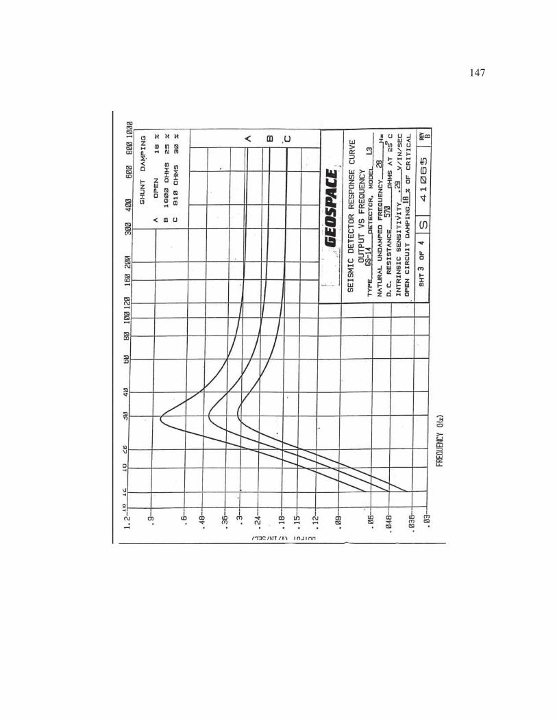
147

148
B.9. HS-1 Geophone Data Sheet

149

150

151
B.10. UC-7420 Data Sheet
1 w w w. m o x a . c o m i n f o @ m o x a . c o m
Embedded Computers
UC-7410/7420 SeriesRISC ready-to-run computers with 8 serial ports, dual LANs, USB, PCMCIA, CompactFlash, web server
The UC-7410/7420 Series RISC-based ready-to-run Linux and WinCE computers are designed for embedded applications. The computers feature 8 RS-232/422/485 serial ports, a PCMCIA interface for wireless LAN communication, CompactFlash, and USB ports for adding external memory. The built-in firewall, VPN, and web server make these computers ideal for applications that require a web server and front-end controller in the industrial embedded system.
Front View
The pre-installed open-standard Linux or WinCE OS operating system provide a convenient platform for software development. In fact, software written for a desktop PC can be ported as is to the UC-7410/7420 platform using readily available development tools, and the code can be stored in the UC-7410/7420’s Flash memory. System integrators will find it easy to use the UC-7410/7420 computers as part of distributed control systems based on embedded technology.
128 MB RAM onboard, 32 MB flash ›8 RS-232/422/485 serial ports ›Dual 10/100 Mbps LANs for network redundancy ›USB 2.0 host ›CompactFlash socket for storage expansion ›PCMCIA supporting WLAN, GPRS, UMTS, HSDPA ›LCM display and keypad for HMI ›Built-in firewall and VPN function ›Apache web server supporting PHP and XML ›Ready-to-run Linux or WinCE 5.0 platform ›DIN-rail or wallmount installation ›Robust, fanless design ›
Reset
P1RS-232/422/485 P2 P3 P4 P5 P6 P7 P8
Reset toDefault
D/O D/I
(RS-232/422/485)
1 2 3 5 64 7 8 1 2 3 5 64 7 8
Reset to Default8-ch Digital Output
Hardware Reset
(UC-7408) (UC-7408)8-ch Digital Input
Serial Port x 8 RJ45
(UC-7420/7410/7408)
Overview
Appearance

152
2 w w w. m o x a . c o m i n f o @ m o x a . c o m
Embedded Computers
Rear ViewDC 12-48V
USBLAN1 LAN2 Console
V+ V-
PCMCIA
CF
12-48 VDC Power Input
CF x 1
PCMCIA x 1USB 2.0 Host x 2, A Type Connector
USB 1.1 Client x 1,miniB Connector
RS-232Console Port10/100 Mbps
Ethernet x 2
(UC-7420)(UC-7420/7408/7402)
(UC-7420/7408/7402)
ComputerCPU: UC-7410/7420: Intel XScale IXP422 266 MHz UC-7410/7420 Plus: Intel XScale IXP425 533 MHzOS (pre-installed): Embedded Linux or Windows CE 5.0DRAM: 128 MB onboardFlash: 32 MB onboardPCMCIA: Cardbus card and 16-bit PCMCIA 2.1 ro JEIDA 4.2 card (UC-7420 only)USB:
StorageStorage Expansion: CompactFlash socket (UC-7420, UC-7420 Plus)Ethernet InterfaceLAN: 2 auto-sensing 10/100 Mbps ports (RJ45)Magnetic Isolation Protection: 1.5 KV built-inSerial InterfaceSerial Standards: RS-232/422/485 software-selectable (8-pin RJ45), 8 portsESD Protection: 15 KV for all signalsConsole Port: RS-232 (all signals), RJ45 connector, supports PPPSerial Communication ParametersData Bits: 5, 6, 7, 8Stop Bits: 1, 1.5, 2Parity: None, Even, Odd, Space, MarkFlow Control: RTS/CTS, XON/XOFF, ADDC® (automatic data direction control) for RS-485Baudrate: 50 bps to 921.6 Kbps (supports non-standard baudrates; see user’s manual for details)Serial SignalsRS-232: TxD, RxD, DTR, DSR, RTS, CTS, DCD, GNDRS-422: TxD+, TxD-, RxD+, RxD-, GNDRS-485-4w: TxD+, TxD-, RxD+, RxD-, GNDRS-485-2w: Data+, Data-, GNDLEDsSystem: OS Ready, Console (TxD/RxD)LAN: 10M/100M x 2Serial: TxD x 8, RxD x 8 (UC-7408/7410/7420, UC-7408/7410/7420 Plus only)Physical CharacteristicsHousing: SECC sheet metal (1 mm)Weight: UC-7410: 810 g UC-7420: 875 gDimensions: 197 x 44 x 125 mm (7.76 x 1.73 x 4.92 in)Mounting: DIN-Rail, wall
Environmental LimitsOperating Temperature: -10 to 60°C (14 to 140°F)Operating Humidity: 5 to 95% RHStorage Temperature: -20 to 80°C (-4 to 176°F)Anti-vibration: 1 g @ IEC-68-2-6, sine wave (resonance search), 5-500 Hz, 1 Oct/min, 1 cycle, 13 min 17 sec per axisAnti-Shock: 5 g @ IEC-68-2-27, half sine wave, 30 msPower RequirementsInput Voltage: 12 to 48 VDCPower Consumption: UC-7410: 10 W
UC-7420: 11 W
Regulatory ApprovalsEMC: CE (EN55022 Class A, EN61000-3-2 Class A, EN61000-3-3, EN55024), FCC (Part 15 Subpart B, CISPR 22 Class A)Safety: UL/cUL (UL60950-1, CSA C22.2 No. 60950-1-03), TÜV (EN60950-1)ReliabilityAlert Tools: Built-in buzzer and RTC (real-time clock)Automatic Reboot Trigger: Built-in WDT (watchdog timer)WarrantyWarranty Period: 5 yearsDetails: See www.moxa.com/warranty
Hardware Specifications
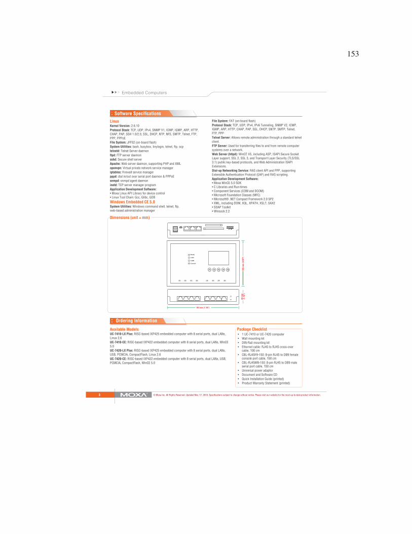
153
3
Embedded Computers
© Moxa Inc. All Rights Reserved. Updated Mar. 17, 2010. Specifications subject to change without notice. Please visit our website for the most up-to-date product information.
LinuxKernel Version: 2.6.10Protocol Stack: TCP, UDP, IPv4, SNMP V1, ICMP, IGMP, ARP, HTTP, CHAP, PAP, SSH 1.0/2.0, SSL, DHCP, NTP, NFS, SMTP, Telnet, FTP, PPP, PPPoEFile System: JFFS2 (on-board flash)System Utilities: bash, busybox, tinylogin, telnet, ftp, scptelnetd: Telnet Server daemonftpd: FTP server daemonsshd: Secure shell serverApache: Web server daemon, supporting PHP and XMLopenvpn: Virtual private network service manageriptables: Firewall service managerpppd: dial in/out over serial port daemon & PPPoEsnmpd: snmpd agent daemoninetd: TCP server manager programApplication Development Software:
Windows Embedded CE 5.0System Utilities: Windows command shell, telnet, ftp, web-based administration manager
File System: FAT (on-board flash)Protocol Stack: TCP, UDP, IPv4, IPv6 Tunneling, SNMP V2, ICMP, IGMP, ARP, HTTP, CHAP, PAP, SSL, DHCP, SNTP, SMTP, Telnet, FTP, PPPTelnet Server: Allows remote administration through a standard telnet client.FTP Server: Used for transferring files to and from remote computer systems over a network.Web Server (httpd): WinCE IIS, including ASP, ISAPI Secure Socket Layer support, SSL 2, SSL 3, and Transport Layer Security (TLS/SSL 3.1) public key-based protocols, and Web Administration ISAPI Extensions.Dial-up Networking Service: RAS client API and PPP, supporting Extensible Authentication Protocol (EAP) and RAS scripting.Application Development Software:
197 mm [7.76"]
]"29.4[ m
m 521m
m 44]"37.1[
Software Specifications
Dimensions (unit = mm)
Package Checklist1 UC-7410 or UC-7420 computerWall mounting kitDIN-Rail mounting kitEthernet cable: RJ45 to RJ45 cross-over cable, 100 cmCBL-RJ45F9-150: 8-pin RJ45 to DB9 female console port cable, 150 cmCBL-RJ45M9-150: 8-pin RJ45 to DB9 male serial port cable, 150 cmUniversal power adaptorDocument and Software CD
Product Warranty Statement (printed)
Available ModelsUC-7410-LX Plus: RISC-based IXP425 embedded computer with 8 serial ports, dual LANs, Linux 2.6UC-7410-CE: RISC-based IXP422 embedded computer with 8 serial ports, dual LANs, WinCE 5.0UC-7420-LX Plus: RISC-based IXP425 embedded computer with 8 serial ports, dual LANs, USB, PCMCIA, CompactFlash, Linux 2.6UC-7420-CE: RISC-based IXP422 embedded computer with 8 serial ports, dual LANs, USB, PCMCIA, CompactFlash, WinCE 5.0
Ordering Information

154
B.11. Bus Resistor Data Sheet
4600X Series - Thick Film Conformal SIPs
Specifications are subject to change without notice.Customers should verify actual device performance in their specific applications.
Product CharacteristicsResistance Range
......................10 ohms to 10 megohmsMaximum Operating Voltage..........100 VTemperature Coefficient of Resistance
50 � to 2.2 M�................±100 ppm/°Cbelow 50 � ......................±250 ppm/°Cabove 2.2 M�..................±250 ppm/°C
TCR Tracking .........................50 ppm/°C maximum; equal values
Resistor Tolerance ................See circuitsInsulation Resistance
..................10,000 megohms minimumDielectric Withstanding Voltage
.............................................200 VRMSOperating Temperature
.................................-55 °C to +125 °C
Environmental CharacteristicsTESTS PER MIL-STD-202.........�R MAX.Short Time Overload..................±0.25 %Load Life ....................................±1.00 %Moisture Resistance ..................±0.50 %Resistance to Soldering Heat ....±0.25 %Terminal Strength.......................±0.25 %Thermal Shock...........................±0.25 %
Physical CharacteristicsFlammability .........Conforms to UL94V-0Body Material........................Epoxy resinStandard Packaging
....................Bulk, Ammo-pak available
WA
TTS
AMBIENT TEMPERATURE ( C )°0 70 125
3.50
3.00
2.50
2.00
1.50
1.00
.50
25
4612X
4608X
4606X
4614X
4604X
4610X
Package Power Ratings (Watts)
Ambient AmbientTemperature Temperature
Pkg. 70 °C Pkg. 70 °C
4604X 0.50 4610X 1.254605X 0.63 4611X 1.384606X 0.75 4612X 1.504607X 0.88 4613X 1.634608X 1.00 4614X 1.754609X 1.13
AMAXIMUM
PIN #1REF.
5.08(.200)MAX.
3.43 +.38/ -.508(.135 +.015/ -.020)
1.24(.049)
MAX.BOTH ENDS
.508 ± .050(.020 ± .002)TYP.
2.54 ± .07(.100 ± .003*)
TYP.NON-ACCUM.
2.49(.098) MAX.
.254 ± .050(.010 ± .002) MAX.
Maximum package length is equal to 2.54mm (.100") times the number of pins, less .005mm (.002").
Governing dimensions are in metric. Dimensions in parentheses are inches and are approximate.
*Terminal centerline to centerline measurements made at point ofemergence of the lead from the body.
NUMBER OF PINS6X-2-222 YYWW
CIRCUIT
RESISTANCECODE
PIN ONEINDICATOR
MANUFACTURER'STRADEMARK
DATE CODE
Typical Part MarkingRepresents total content. Layout may vary.
How To Order
46 06 X - 101 - 222 __ LF Model(46 = Conformal SIP)
Number of Pins
Physical Configuration(X = Thick Film Low Profile)
Electrical Configuration• 101 = Bussed• 102 = Isolated• 104 = Dual Terminator• AP1 = Bussed Ammo**• AP2 = Isolated Ammo**• AP4 = Dual Ammo**
Resistance Code• First 2 digits are significant• Third digit represents the number of
zeros to follow.
Resistance Tolerance• Blank = ±2 % (see “Resistance Tolerance”
on next page for resistance range)• F = ±1 % (100 ohms - 5 megohms)
Terminations• All electrical configurations EXCEPT 104 & AP4:
LF = Sn/Ag/Cu-plated (RoHS compliant)• ONLY electrical configurations 104 & AP4:
L = Sn/Ag/Cu-plated (RoHS compliant)
Consult factory for other available options.
**Available for packages with 10 pins or less.
Part Number Part Number
4606X-101-RC 6X-1-RC
4608X-102-RC 8X-2-RC
4610X-104-RC/RC 10X-4-RC/RC
RC = ohmic value, 3-digit resistance code.
Pin A MaximumCount mm (Inches)
4 10.11 (.398)5 12.65 (.498)6 15.19 (.598)7 17.73 (.698)8 20.27 (.798)9 22.81 (.898)
10 25.35 (.998)11 27.89 (1.098)12 30.43 (1.198)13 32.97 (1.298)14 35.51 (1.398)
Package Power Temp. Derating Curve Product Dimensions
Features ■ RoHS compliant*)■ Low profile is compatible with DIPs■ Wide assortment of pin packages
enhances design flexibility■ Ammo-pak packaging available■ Recommended for rosin flux and solvent
clean or no clean flux processes
■ Marking on contrasting background forpermanent identification
*RoH
S COMPLIANT
*RoHS Directive 2002/95/EC Jan 27 2003 including Annex
For Standard Values Used in Capacitors,Inductors, and Resistors, click here.

155
Specifications are subject to change without notice.Customers should verify actual device performance in their specific applications.
Isolated Resistors (102 Circuit)Model 4600X-102-RC4, 6, 8, 10, 12, 14 Pin
Bussed Resistors (101 Circuit)Model 4600X-101-RC4 through 14 Pin
Dual Terminator (104 Circuit)Model 4600X-104-R1/R24 through 14 Pin
1 4 6 12 14
...
1 14
1 8
R2
R1
R2
R1
R2
R1
R2
R1
R2
R1
R2
R1
These models incorporate 2 to 7 isolated thick-film resistors of equalvalue, each connected between twopins.
Resistance Tolerance10 ohms to 49 ohms ...................±1 ohm50 ohms to 5 megohms.................±2 %*Above 5 megohms..........................±5 %
Power Rating per ResistorAt 70 °C ...................................0.30 watt
Power Temperature Derating Curve
WA
TTS
AMBIENT TEMPERATURE ( C )°0 70 125
.50
.40
.30
.20
.10
25
.60
These models incorporate 3 to 13thick-film resistors of equal value, eachconnected between a common bus (pin 1) and a separate pin.
Resistance Tolerance10 ohms to 49 ohms ...................±1 ohm50 ohms to 5 megohms.................±2 %*Above 5 megohms..........................±5 %
Power Rating per ResistorAt 70 °C ...................................0.20 watt
Power Temperature Derating Curve
WA
TTS
AMBIENT TEMPERATURE ( C )°0 70 125
.50
.40
.30
.20
.10
25
.60
The 4608X-104 (shown above) is an 8-pin configuration and terminates 6 lines. Pins 1 and 8 are common for ground andpower, respectively. Twelve thick-filmresistors are paired in series betweenthe common lines (pins 1 and 8).
Resistance ToleranceBelow 100 ohms........................±2 ohms100 ohms to 5 megohms...............±2 %*Above 5 megohms..........................±5 %
Power Rating per ResistorAt 70 °C ...................................0.20 watt
Power Temperature Derating Curve
WA
TTS
AMBIENT TEMPERATURE ( C )°0 70 125
.50
.40
.30
.20
.10
25
.60
Popular Resistance Values (101, 102 Circuits)**
* ±1 % TOLERANCE IS AVAILABLE BY ADDING SUFFIX CODE “F” AFTER THE RESISTANCE CODE.
**NON-STANDARD VALUES AVAILABLE, WITHIN RESISTANCE RANGE.
Ohms Code Ohms Code Ohms Code Ohms Code Ohms Code10 100 180 181 1,800 182 15,000 153 120,000 12422 220 220 221 2,000 202 18,000 183 150,000 15427 270 270 271 2,200 222 20,000 203 180,000 18433 330 330 331 2,700 272 22,000 223 220,000 22439 390 390 391 3,300 332 27,000 273 270,000 27447 470 470 471 3,900 392 33,000 333 330,000 33456 560 560 561 4,700 472 39,000 393 390,000 39468 680 680 681 5,600 562 47,000 473 470,000 47482 820 820 821 6,800 682 56,000 563 560,000 564
100 101 1,000 102 8,200 822 68,000 683 680,000 684120 121 1,200 122 10,000 103 82,000 823 820,000 824150 151 1,500 152 12,000 123 100,000 104 1,000,000 105
Popular Resistance Values (104 Circuit)**
Resistance(Ohms) Code
R1 R2 R1 R2
160 240 161 241180 390 181 391220 270 221 271220 330 221 331330 390 331 391330 470 331 471
3,000 6,200 302 622
4600X Series - Thick Film Conformal SIPs
REV. 12/06
For information on specific applications,download Bourns’ application notes:DRAM ApplicationsDual Terminator Resistor NetworksR/2R Ladder NetworksSCSI Applications

156
B.12. Conductive Pen Data Sheet
TDS # CW2200
PRODUCT DESCRIPTION
CircuitWorks� Conductive Pen makes instant highly conductive silver traces on circuit boards. CW2200 is used in prototype, rework, and repair of circuit boards by linking components, repairing defective traces, and making smooth jumpers. The silver traces dry in minutes and have excellent adhesion to most electronic materials. Engineers, repair technicians, and manufacturers will find that the CircuitWorks� Conductive Pen speeds project completion and cuts rework time.
� Single component system � High electrical conductivity � Fast drying � Highly adherent to circuit boards � Operating temperature to 400�F (205�C)
TYPICAL APPLICATIONS CircuitWorks� Conductive Pen may be used for electronics applications including:
� Circuit Trace Repair � Solderless Linking of Components � EMI Shielding � Solderable Terminations � Quick Prototype Modifications
CHEMTRONICS�
Technical Data Sheet
CircuitWorks� Conductive Pen
TYPICAL PRODUCT DATA AND PHYSICAL PROPERTIES
Composition Material Silver Filled Polymer Silver Particle Size 10-15 microns Color Silver Gray Setting Rate <2mm/hr. Properties Conductivity 0.02-0.05 ohms/sq/mil 0.00005-0.000125 ohm cm Max. Temperature 400�F (205�C) Tack-Free Time @ 25�C 3 to 5 Minutes Cure Time @ 25�C 20 to 30 Minutes Solder Wetting 2 to 3 Seconds Electrical Conductivity Excellent Adhesion Excellent Flexibility Good Chemical Resistance Good Tip Diameters MTP 0.8 mm (0.03 inches) STP 1.2 mm (0.05 inches) Shelflife 12 months
COMPATIBILITYCircuitWorks� Conductive Pen material has excellent compatibility with materials used in printed circuit board fabrication. As with any chemical system, compatibility with the substrate must be determined on a non-critical area prior to use.

157
USAGE INSTRUCTIONSRead MSDS carefully prior to use.
Cleaning: For best adhesion, clean board with one of Chemtronics Electro-Wash� or Pow-R-Wash�solvents in order to remove any surface contamination which may prevent adequate material contact.
Mixing: Although this system has been formulated to resist hard-packing, it should be shaken vigorously for 30 seconds to insure the proper dispersion of the silver flakes. If pen has been allowed to sit idle for a long period of time, the mixing ball may seize in the barrel. To free the ball use force to tap the barrel end of the pen until the ball begins to move inside the pen.
Application: The conductive ink is dispensed through the CircuitWorks� Conductive Pen. Squeezing the pen body while pressing down on the surface will allow the material to flow, enabling the trace to be drawn. Practice with the pen before attempting detail work. The bulk form of this material may be applied by brushing, banding, or automatic dispensing equipment.
Thinning: The conductive ink has been optimized for the CircuitWorks� Conductive Pen and thinning is not normally necessary. However, Butyl Acetate may be added with thorough mixing to make slight adjustments for ease of application in the bulk form.
Clean-up/Removal: The conductive ink may be cleaned or removed using a strong organic solvent such as Chemtronics� Electro-Wash� PX.
Curing: Tack-free in 3 to 5 minutes at room temperature. Achieves electrical conductivity within 30 minutes. Heat cure for 5 minutes at 250 to 300�F (120 to 150�C) for maximum conductivity, durability and chemical resistance.
Soldering: Low temperature soldering is possible to the heat-cured silver conductive traces if done at 350�F (177�C) for <5 seconds.
AVAILABILITY
CW2200STP 8.5 g (0.3 oz.), Standard 1.2 mm tip CW2200MTP 8.5g (0.3 oz.), MicroTip 0.8 mm tip
TECHNICAL & APPLICATION ASSISTANCEChemtronics� provides a technical hotline to answer your technical and application related questions. The toll free number is: 1-800-TECH-401.
NOTE:This information is believed to be accurate. It is intended for professional end users having the skills to evaluate and use the data properly. ITW CHEMTRONICS� does not guarantee the accuracy of the data and assumes no liability in connection with damages incurred while using it.
MANUFACTURED BY: ITW CHEMTRONICS�
8125 COBB CENTER DRIVE KENNESAW, GA 30152 1-770-424-4888 REV. F (06/09)
DISTRIBUTED BY:

158
B.13. “Bridge Paint” Data Sheet
Revised 2/10
MACROPOXY® 646FAST CURE EPOXY
PART A B58-600 SERIES PART B B58V600 HARDENER
Protective &
MarineCoatings
4.53
www.sherwin-williams.com/protective
PRODUCT DESCRIPTIONMACROPOXY 646 FAST CURE EPOXY is a high solids, high build, fast drying, polyamide epoxy designed to protect steel and concrete in industrial exposures. Ideal for maintenance painting and fabrica-tion shop applications. The high solids content ensures adequate protection of sharp edges, corners, and welds. This product can be applied directly to marginally prepared steel surfaces.• Low VOC • Chemical resistant• Low odor • Abrasion resistant• Outstanding application properties
PRODUCT CHARACTERISTICSFinish: Semi-GlossColor: Mill White, Black and a wide range of colors available through tintingVolume Solids: 72% ± 2%, mixed, Mill WhiteWeight Solids: 85% ± 2%, mixed, Mill WhiteVOC (EPA Method 24): Unreduced: <250 g/L; 2.08 lb/gal mixed Reduced 10%: <300 g/L; 2.50 lb/galMix Ratio: 1:1 by volume
Recommended Spreading Rate per coat:Minimum Maximum
Wet mils (microns) 7.0 175 13.5 338Dry mils (microns) 5.0* 125 10.0* 250~Coverage sq ft/gal (m2/L) 116 2.8 232 5.7Theoretical coverage sq ft/gal (m2/L) @ 1 mil / 25 microns dft 1152 28.2*May be applied at 3.0-10.0 mils dft as an intermediate coat. Refer to Recommended Systems (page 2).
NOTE: Brush or roll application may require multiple coats to achieve maximum fi lm thickness and uniformity of appearance.
Drying Schedule @ 7.0 mils wet (175 microns):@ 35°F/1.7°C @ 77°F/25°C @ 100°F/38°C
50% RHTo touch: 4-5 hours 2 hours 1.5 hoursTo handle: 48 hours 8 hours 4.5 hoursTo recoat:
minimum: 48 hours 8 hours 4.5 hoursmaximum: 1 year 1 year 1 year
To cure:Service: 10 days 7 days 4 days
Immersion: 14 days 7 days 4 daysIf maximum recoat time is exceeded, abrade surface before recoating.
Drying time is temperature, humidity, and fi lm thickness dependent.Paint temperature must be at least 40°F (4.5°C) minimum.Pot Life: 10 hours 4 hours 2 hoursSweat-in-time: 30 minutes 30 minutes 15 minutes
When used as an intermediate coat as part of a multi-coat system:
Drying Schedule @ 5.0 mils wet (125 microns):@ 35°F/1.7°C @ 77°F/25°C @ 100°F/38°C
50% RHTo touch: 3 hours 1 hour 1 hourTo handle: 48 hours 4 hours 2 hoursTo recoat:
minimum: 16 hours 4 hours 2 hoursmaximum: 1 year 1 year 1 year
continued on back
PRODUCT CHARACTERISTICS (CONT'D)
Shelf Life: 36 months, unopenedStore indoors at 40°F (4.5°C)to 100°F (38°C).
Flash Point: 91°F (33°C), TCC, mixedReducer/Clean Up:In California:
Reducer, R7K15Reducer R7K111 or Oxsol 100
RECOMMENDED USES• Marine applications• Fabrication shops • Refi neries• Pulp and paper mills • Chemical plants• Power plants • Tank exteriors• Offshore platforms • Water treatment plants• Mill White and Black are acceptable for immersion use for salt
water and fresh water, not acceptable for potable water• Suitable for use in USDA inspected facilities• Conforms to AWWA D102-03 OCS #5• Conforms to MPI # 108
PERFORMANCE CHARACTERISTICS
Substrate*: SteelSurface Preparation*: SSPC-SP10/NACE 2System Tested*:
1 ct. Macropoxy 646 Fast Cure @ 6.0 mils (150 microns) dft*unless otherwise noted belowTest Name Test Method Results
Abrasion Resistance ASTM D4060, CS17 wheel, 1000 cycles, 1 kg load
84 mg loss
AcceleratedWeathering-QUV1
ASTM D4587, QUV-A,12,000 hours Passes
Adhesion ASTM D4541 1,037 psi
Corrosion Weathering1 ASTM D5894, 36 cycles, 12,000 hours
Rating 10 per ASTM D714 for blistering; Rating 9 per ASTM D610 per rusting
Direct Impact Resistance ASTM D2794 30 in. lb.Dry Heat Resistance ASTM D2485 250°F (121°C)Exterior Durability 1 year at 45° South Excellent, chalks
Flexibility ASTM D522, 180° bend, 3/4" mandrel Passes
Humidity Resistance ASTM D4585, 6000 hours
No blistering, cracking, or rusting
Immersion 1 year fresh and salt water
Passes, no rusting, blistering, or loss of adhesion
Irradiation-Effectson Coatings used in Nuclear Power Plants
ANSI 5.12 / ASTM D4082-89 Passes
Pencil Hardness ASTM D3363 3H
Salt Fog Resistance1 ASTM B117, 6,500 hours
Rating 10 per ASTM D610 for rusting; Rating 9 per ASTM D1654 for corrosion
Slip Coeffi cient, Mill White
AISC Specification for Struc-tural Joints Using ASTM A325 or ASTM A490 Bolts
Class A, 0.36
Water Vapor Permeance ASTM D1653, Method B 1.16 US perms
Epoxy coatings may darken or discolor following application and curing.
Footnotes:1 Zinc Clad II Plus Primer

159
4.53
MACROPOXY® 646FAST CURE EPOXY
PART A B58-600 SERIES PART B B58V600 HARDENER
Protective &
MarineCoatings
www.sherwin-williams.com/protective
SURFACE PREPARATION
Surface must be clean, dry, and in sound condition. Remove all oil, dust, grease, dirt, loose rust, and other foreign material to ensure adequate adhesion.
Refer to product Application Bulletin for detailed surface preparation in-formation.Minimum recommended surface preparation: Iron & Steel Atmospheric: SSPC-SP2/3 Immersion: SSPC-SP10/NACE 2, 2-3 mil (50-75 micron) profi le Aluminum: SSPC-SP1 Galvanizing: SSPC-SP1 Concrete & Masonry Atmospheric: SSPC-SP13/NACE 6, or ICRI 03732, CSP 1-3 Immersion: SSPC-SP13/NACE 6-4.3.1 or 4.3.2, or ICRI 03732, CSP 1-3
Surface Preparation StandardsCondition of Surface
ISO 8501-1BS7079:A1
Swedish Std.SIS055900 SSPC NACE
White Metal Sa 3 Sa 3 SP 5 1Near White Metal Sa 2.5 Sa 2.5 SP 10 2Commercial Blast Sa 2 Sa 2 SP 6 3Brush-Off Blast Sa 1 Sa 1 SP 7 4Hand Tool Cleaning Rusted C St 2 C St 2 SP 2 -
Pitted & Rusted D St 2 D St 2 SP 2 -Power Tool Cleaning Rusted C St 3 C St 3 SP 3 -
Pitted & Rusted D St 3 D St 3 SP 3 -
TINTINGTint Part A with Maxitoners at 150% strength. Five minutes minimum mix-ing on a mechanical shaker is required for complete mixing of color.
Tinting is not recommended for immersion service.
APPLICATION CONDITIONSTemperature: 35°F (1.7°C) minimum, 120°F (49°C) maximum (air and surface) 40°F (4.5°C) minimum, 120°F (49°C)
maximum (material) At least 5°F (2.8°C) above dew pointRelative humidity: 85% maximumRefer to product Application Bulletin for detailed application information.
ORDERING INFORMATIONPackaging: Part A: 1 gallon (3.78L) and 5 gallon (18.9L) containers Part B: 1 gallon (3.78L) and 5 gallon (18.9L) containersWeight: 12.9 ± 0.2 lb/gal ; 1.55 Kg/L mixed, may vary by color
SAFETY PRECAUTIONS
Refer to the MSDS sheet before use.Published technical data and instructions are subject to change without notice.Contact your Sherwin-Williams representative for additional technical data and instructions.
WARRANTYThe Sherwin-Williams Company warrants our products to be free of manufactur-ing defects in accord with applicable Sherwin-Williams quality control procedures. Liability for products proven defective, if any, is limited to replacement of the defec-tive product or the refund of the purchase price paid for the defective product as determined by Sherwin-Williams. NO OTHER WARRANTY OR GUARANTEE OF ANY KIND IS MADE BY SHERWIN-WILLIAMS, EXPRESSED OR IMPLIED, STATUTORY, BY OPERATION OF LAW OR OTHERWISE, INCLUDING MER-CHANTABILITY AND FITNESS FOR A PARTICULAR PURPOSE.
PRODUCT INFORMATION
RECOMMENDED SYSTEMS Dry Film Thickness / ct.
Mils (Microns)Immersion and atmospheric:Steel:2 cts. Macropoxy 646 5.0-10.0 (125-250)Concrete/Masonry, smooth:2 cts. Macropoxy 646 5.0-10.0 (125-250)Concrete Block:1 ct. Kem Cati-Coat HS Epoxy 10.0-20.0 (250-500) Filler/Sealer
as needed to fi ll voids and provide a continuous substrate.2 cts. Macropoxy 646 5.0-10.0 (125-250)Atmospheric:Steel:(Shop applied system, new construction, AWWA D102-03, can also beused at 3 mils minimum dft when used as an intermediate coat as partof a multi-coat system)1 ct. Macropoxy 646 Fast Cure Epoxy 3.0-6.0 (75-150)1-2 cts. of recommended topcoatSteel:1 ct. Recoatable Epoxy Primer 4.0-6.0 (100-150)2 cts. Macropoxy 646 5.0-10.0 (125-250)Steel:1 ct. Macropoxy 646 4.0-6.0 (100-150)1-2 cts. Acrolon 218 Polyurethane 3.0-6.0 (75-150)
or Hi-Solids Polyurethane 3.0-5.0 (75-125)or SherThane 2K Urethane 2.0-4.0 (50-100)or Hydrogloss 2.0-4.0 (50-100)
Steel:2 cts. Macropoxy 646 5.0-10.0 (125-250)1-2 cts. Tile-Clad HS Epoxy 2.5-4.0 (63-100)Steel:1 ct. Zinc Clad II Plus 3.0-6.0 (75-150)1 ct. Macropoxy 646 3.0-10.0 (75-250)1-2 cts. Acrolon 218 Polyurethane 3.0-6.0 (75-150)Steel:1 ct. Zinc Clad III HS 3.0-5.0 (75-125) or Zinc Clad IV 3.0-5.0 (75-125)1 ct. Macropoxy 646 3.0-10.0 (75-250)1-2 cts. Acrolon 218 Polyurethane 3.0-6.0 (75-150)Aluminum:2 cts. Macropoxy 646 5.0-10.0 (125-250)Galvanizing:2 cts. Macropoxy 646 5.0-10.0 (125-250)The systems listed above are representative of the product's use, other systems may be appropriate.
DISCLAIMERThe information and recommendations set forth in this Product Data Sheet are based upon tests conducted by or on behalf of The Sherwin-Williams Company. Such information and recommendations set forth herein are subject to change and pertain to the product offered at the time of publication. Consult your Sherwin-Williams representative to obtain the most recent Product Data Information and Application Bulletin.

160
Revised 2/10
MACROPOXY® 646FAST CURE EPOXY
PART A B58-600 SERIES PART B B58V600 HARDENER
Protective &
MarineCoatings
4.53
www.sherwin-williams.com/protective
SURFACE PREPARATIONS
Surface must be clean, dry, and in sound condition. Remove all oil, dust, grease, dirt, loose rust, and other foreign material to ensure adequate adhesion.
Iron & Steel, Atmospheric Service:Minimum surface preparation is Hand Tool Clean per SSPC-SP2. Remove all oil and grease from surface by Solvent Cleaning per SSPC-SP1. For better performance, use Commercial Blast Cleaning per SSPC-SP6/NACE 3, blast clean all surfaces using a sharp, angular abrasive for optimum surface profi le (2 mils / 50 microns). Prime any bare steel within 8 hours or before fl ash rusting occurs.Iron & Steel, Immersion Service:Remove all oil and grease from surface by Solvent Cleaning per SSPC-SP1. Minimum surface preparation is Near White Metal Blast Cleaning per SSPC-SP10/NACE 2. Blast clean all surfaces using a sharp, angular abrasive for optimum surface profi le (2-3 mils / 50-75 microns). Remove all weld spatter and round all sharp edges by grind-ing. Prime any bare steel the same day as it is cleaned.AluminumRemove all oil, grease, dirt, oxide and other foreign material by Solvent Cleaning per SSPC-SP1.Galvanized SteelAllow to weather a minimum of six months prior to coating. Solvent Clean per SSPC-SP1 (recommended solvent is VM&P Naphtha). When weathering is not possible, or the surface has been treated with chro-mates or silicates, fi rst Solvent Clean per SSPC-SP1 and apply a test patch. Allow paint to dry at least one week before testing adhesion. If adhesion is poor, brush blasting per SSPC-SP7 is necessary to remove these treatments. Rusty galvanizing requires a minimum of Hand Tool Cleaning per SSPC-SP2, prime the area the same day as cleaned.Concrete and MasonryFor surface preparation, refer to SSPC-SP13/NACE 6, or ICRI 03732, CSP 1-3. Surfaces should be thoroughly clean and dry. Concrete and mortar must be cured at least 28 days @ 75°F (24°C). Remove all loose mortar and foreign material. Surface must be free of laitance, concrete dust, dirt, form release agents, moisture curing membranes, loose cement and hardeners. Fill bug holes, air pockets and other voids with Steel-Seam FT910. Concrete, Immersion Service:For surface preparation, refer to SSPC-SP13/NACE 6, Section 4.3.1 or 1.3.2 or ICRI 03732, CSP 1-3.Always follow the standard methods listed below:ASTM D4258 Standard Practice for Cleaning Concrete.ASTM D4259 Standard Practice for Abrading Concrete.ASTM D4260 Standard Practice for Etching Concrete.ASTM F1869 Standard Test Method for Measuring Moisture Vapor Emission Rate of Concrete.SSPC-SP 13/Nace 6 Surface Preparation of Concrete.ICRI 03732 Concrete Surface Preparation.Previously Painted SurfacesIf in sound condition, clean the surface of all foreign material. Smooth, hard or glossy coatings and surfaces should be dulled by abrading the surface. Apply a test area, allowing paint to dry one week before testing adhesion. If adhesion is poor, or if this product attacks the previous fi nish, removal of the previous coating may be necessary. If paint is peeling or badly weathered, clean surface to sound substrate and treat as a new surface as above.
Surface Preparation StandardsCondition of Surface
ISO 8501-1BS7079:A1
Swedish Std.SIS055900 SSPC NACE
White Metal Sa 3 Sa 3 SP 5 1Near White Metal Sa 2.5 Sa 2.5 SP 10 2Commercial Blast Sa 2 Sa 2 SP 6 3Brush-Off Blast Sa 1 Sa 1 SP 7 4Hand Tool Cleaning Rusted C St 2 C St 2 SP 2 -
Pitted & Rusted D St 2 D St 2 SP 2 -Power Tool Cleaning Rusted C St 3 C St 3 SP 3 -
Pitted & Rusted D St 3 D St 3 SP 3 -
APPLICATION BULLETIN
APPLICATION CONDITIONS
Temperature: 35°F (1.7°C) minimum, 120°F (49°C) maximum (air and surface) 40°F (4.5°C) minimum, 120°F (49°C)
maximum (material) At least 5°F (2.8°C) above dew point
Relative humidity: 85% maximum
APPLICATION EQUIPMENT
The following is a guide. Changes in pressures and tip sizes may be needed for proper spray characteristics. Always purge spray equipment before use with listed reducer. Any reduction must be compliant with existing VOC regulations and compatible with the existing environmental and application conditions.
Reducer/Clean Up ...........Reducer R7K15 In California ....................Reducer R7K111
Airless Spray Pump..............................30:1 Pressure.........................2800 - 3000 psi Hose...............................1/4" ID Tip ...................................017" - .023" Filter ...............................60 mesh Reduction .......................As needed up to 10% by volume
Conventional Spray Gun ................................DeVilbiss MBC-510 Fluid Tip .........................E Air Nozzle.......................704 Atomization Pressure .....60-65 psi Fluid Pressure ................10-20 psi Reduction .......................As needed up to 10% by volume Requires oil and moisture separators
Brush Brush..............................Nylon/Polyester or Natural Bristle Reduction .......................Not recommended
Roller Cover .............................3/8" woven with solvent resistant core Reduction .......................Not recommended
If specifi c application equipment is not listed above, equivalent equipment may be substituted.
continued on back

161
4.53
MACROPOXY® 646FAST CURE EPOXY
PART A B58-600 SERIES PART B B58V600 HARDENER
Protective &
MarineCoatings
www.sherwin-williams.com/protective
APPLICATION BULLETIN
APPLICATION PROCEDURESSurface preparation must be completed as indicated.Mix contents of each component thoroughly with low speed power agitation. Make certain no pigment remains on the bottom of the can. Then combine one part by volume of Part A with one part by volume of Part B. Thoroughly agitate the mixture with power agitation. Allow the material to sweat-in as indicated prior to ap-plication. Re-stir before using.If reducer solvent is used, add only after both components have been thoroughly mixed, after sweat-in.Apply paint at the recommended fi lm thickness and spreading rate as indicated below:
Recommended Spreading Rate per coat:Minimum Maximum
Wet mils (microns) 7.0 175 13.5 338Dry mils (microns) 5.0* 125 10.0* 250~Coverage sq ft/gal (m2/L) 116 2.8 232 5.7Theoretical coverage sq ft/gal (m2/L) @ 1 mil / 25 microns dft 1152 28.2*May be applied at 3.0-10.0 mils dft as an intermediate coat. Refer to Recommended Systems (page 2).
NOTE: Brush or roll application may require multiple coats to achieve maximum fi lm thickness and uniformity of appearance.
Drying Schedule @ 7.0 mils wet (175 microns):@ 35°F/1.7°C @ 77°F/25°C @ 100°F/38°C
50% RHTo touch: 4-5 hours 2 hours 1.5 hoursTo handle: 48 hours 8 hours 4.5 hoursTo recoat:
minimum: 48 hours 8 hours 4.5 hoursmaximum: 1 year 1 year 1 year
To cure:Service: 10 days 7 days 4 days
Immersion: 14 days 7 days 4 daysIf maximum recoat time is exceeded, abrade surface before recoating.
Drying time is temperature, humidity, and fi lm thickness dependent.Paint temperature must be at least 40°F (4.5°C) minimum.Pot Life: 10 hours 4 hours 2 hoursSweat-in-time: 30 minutes 30 minutes 15 minutes
When used as an intermediate coat as part of a multi-coat system:
Drying Schedule @ 5.0 mils wet (125 microns):@ 35°F/1.7°C @ 77°F/25°C @ 100°F/38°C
50% RHTo touch: 3 hours 1 hour 1 hourTo handle: 48 hours 4 hours 2 hoursTo recoat:
minimum: 16 hours 4 hours 2 hoursmaximum: 1 year 1 year 1 year
Application of coating above maximum or below minimum recommended spreading rate may adversely affect coating performance.
CLEAN UP INSTRUCTIONSClean spills and spatters immediately with Reducer R7K15. Clean tools immediately after use with Reducer R7K15. In California use Reducer R7K111. Follow manufacturer's safety recommendations when using any solvent.
PERFORMANCE TIPS
Stripe coat all crevices, welds, and sharp angles to prevent early failure in these areas.
When using spray application, use a 50% overlap with each pass of the gun to avoid holidays, bare areas, and pinholes. If necessary, cross spray at a right angle
Spreading rates are calculated on volume solids and do not include an application loss factor due to surface profi le, roughness or po-rosity of the surface, skill and technique of the applicator, method of application, various surface irregularities, material lost during mixing, spillage, overthinning, climatic conditions, and excessive fi lm build.
Excessive reduction of material can affect fi lm build, appearance, and adhesion.
Do not mix previously catalyzed material with new.
Do not apply the material beyond recommended pot life.
In order to avoid blockage of spray equipment, clean equipment before use or before periods of extended downtime with Reducer R7K15. In California use Reducer R7K111.
Tinting is not recommended for immersion service.
Use only Mil White and Black for immersion service.
Insuffi cient ventilation, incomplete mixing, miscatalyzation, and external heaters may cause premature yellowing.
Excessive fi lm build, poor ventilation, and cool temperatures may cause solvent entrapment and premature coating failure.
Quik-Kick Epoxy Accelerator is acceptable for use. See data page 4.99 for details.
Refer to Product Information sheet for additional performance characteristics and properties.
SAFETY PRECAUTIONSRefer to the MSDS sheet before use.
Published technical data and instructions are subject to change without notice. Contact your Sherwin-Williams representative for additional technical data and instructions.
DISCLAIMERThe information and recommendations set forth in this Product Data Sheet are based upon tests conducted by or on behalf of The Sherwin-Williams Company. Such information and recommendations set forth herein are subject to change and pertain to the product offered at the time of publication. Consult your Sherwin-Williams representative to obtain the most recent Product Data Information and Application Bulletin.
WARRANTYThe Sherwin-Williams Company warrants our products to be free of manufacturing defects in accord with applicable Sherwin-Williams quality control procedures. Liability for products proven defective, if any, is limited to replacement of the de-fective product or the refund of the purchase price paid for the defective product as determined by Sherwin-Williams. NO OTHER WARRANTY OR GUARANTEE OF ANY KIND IS MADE BY SHERWIN-WILLIAMS, EXPRESSED OR IMPLIED, STATUTORY, BY OPERATION OF LAW OR OTHERWISE, INCLUDING MER-CHANTABILITY AND FITNESS FOR A PARTICULAR PURPOSE.