wireless sensor networks for clinical applications in ... · 4 wireless sensor networks for...

Carlos Jorge Enes Capitão de Abreu

June 2014UM

inho

|201

4

Wireless Sensor Networks for ClinicalApplications in Smart Environments

Universidade do Minho

Escola de Engenharia

Car

los

Jorg

e Ene

s C

apitã

o de

Abr

euW

ire

less

Se

nso

r N

etw

ork

s fo

r C

lin

ica

l A

pp

lica

tio

ns

in S

ma

rt E

nvi

ron

me

nts

Doctoral Program on Biomedical Engineering

PhD thesis developed under the scientific supervision of:

Prof. Doutor Paulo Mateus Mendes

Prof. Doutor Manuel Alberto Pereira Ricardo

Carlos Jorge Enes Capitão de Abreu

June 2014

Wireless Sensor Networks for ClinicalApplications in Smart Environments

Universidade do Minho

Escola de Engenharia

STATEMENT OF INTEGRITY

I hereby declare having conducted my thesis with integrity. I confirm that I have not used plagiarism or any

form of falsification of results in the process of the thesis elaboration.

I further declare that I have fully acknowledged the Code of Ethical Conduct of the University of Minho.

University of Minho, _____________________________

Full name: _____________________________________________________________________

Signature: ______________________________________________________________________

iii

to my lovely wife Irene, and my wonderful children Ana and Miguel

v

Acknowledgment

I would like to express my thanks and appreciation to my advisor, Professor Paulo Mendes, for

his guidance throughout this journey. I am grateful for his sage advices and for inspiring me to

explore the many topics that sparked my imagination.

I would also like to express my appreciation to my co-advisor, Professor Manuel Ricardo, for his

support and guidance during this work.

I would also like to thank my friend, Professor Francisco Miranda, for his help developing the

mathematical framework for this work.

I would also like to thank Drª Maria Emília Vilarinho, Drª Cristina Carvalho, and the nursing staff

at Hospital Valentim Ribeiro – without their help, the real-world assessment of my work, would

not have been possible.

I am grateful to Fundação para a Ciência e a Tecnologia, which supported this work under the

PhD grant SFRH/BD/61278/2009.

I am grateful to my parents, José and Maria de Lurdes, for their love and support.

Finally, I have to be grateful, from the bottom of my heart, to the most incredible children and

adorable wife.

vii

Wireless Sensor Networks for Clinical Applications in

Smart Environments

Abstract

Biomedical wireless sensor networks are a key technology to support the development of new

applications and services targeting the domain of healthcare, in particular, regarding data

collection for continuous health monitoring of patients or to help physicians on their diagnosis

and further treatment assessment. Therefore, due to the critical nature of both medical data and

medical applications, such networks have to satisfy demanding quality of service requirements.

Such goals are, nevertheless, negatively influenced by several factors. Those factors can be either

internal (e.g., the network topology and the limited network throughput) or external (e.g., the

characteristics and the use of the network deployment area) to the biomedical wireless sensor

network. Indeed, when designing biomedical wireless sensor network, it should be taken into

consideration numerous aspects of a very different nature.

Despite the efforts made in the last few years to develop quality of service mechanisms targeting

wireless sensor networks and its wide range of applications, the network deployment scenario

can severely restrict the networks ability to provide the required performance. In particular, harsh

environments, such as hospital facilities, can compromise the radio frequency communications

and, consequently, the network’s ability to provide the quality of service required by medical

applications. Furthermore, the impact of such environments on the network performance is hard

to predict and manage due to its random nature. Consequently, network planning and

management, in general or step-down hospital units, is a very hard task. In such context, this

thesis presents a quality of service based network management method to help engineers,

network administrators, and healthcare professionals managing and supervising biomedical

wireless sensor networks.

The proposed quality of service network management method comprises two modules, namely:

the quality of service monitoring module, and the quality of service based admission control

module. The quality of service monitoring module is in charge of continuously monitoring the

relevant metrics used to quantify the performance of each data flow carried by the network, and,

using a mathematical framework, detecting and classifying performance degradation events. By

detecting and classifying quality of service degradation events, the proposed method can be used

to prevent the incorrect operation of the network. Moreover, the information about each

performance degradation event can be used to advise the network administrator to take the

necessary corrective and preventive measures. On its turn, the quality of service based admission

control module can be used to find the best location to add new patients into the network, and

viii

thus allows managing the network in order to find the most favourable network topology to

maximise the quality of service provided by the biomedical wireless sensor network. Moreover,

the quality of service-based admission control module uses the concept of “virtual sensor node”

to mimic the presence of the new sensor nodes (i.e., the new patient) within the network, and by

this way makes it possible to assess the network from a remote location, without the need for the

physical presence of the new patient within the target location.

The quality of service network management method proposed by this thesis was tested using

both simulated and real environments. The field tests were performed in a small-sized hospital

located in Esposende, known as “Hospital Valentim Ribeiro”. In view of the results achieved

during the experiments, the quality of service monitoring module of the proposed method proves

to be a valuable tool for both detection and classification of potential harmful variations in the

quality of service provided by the network, avoiding its degradation to levels where the biomedical

signs would be useless. On its turn, the quality of service based admission control module

demonstrated its ability, not only to control the admission of new patients (i.e., new sensor

nodes) to the biomedical wireless sensor network, but also to find the best location to admit the

new patients within the network. By placing the new sensor nodes on the most favourable

locations, this module is able to optimise the network topology in view of maximising the quality

of service provided by the network.

ix

Rede de Sensores Sem Fios para Aplicações Clínicas em

Ambientes Inteligentes de Assistência à Vida

Resumo

A utilização de redes de sensores sem fios como suporte ao desenvolvimento de novas

aplicações e serviços para a área da saúde é uma realidade crescente, em particular, no que diz

respeito ao desenvolvimento de aplicações para monitorização contínua dos sinais vitais dos

pacientes, com vista à melhoria dos cuidados de saúde prestados. No entanto, devido às

elevadas exigências de qualidade das aplicações e serviços na área da saúde, as redes de

sensores sem fios têm que cumprir requisitos de qualidade de serviço muito exigentes. O

fornecimento de um serviço de elevada qualidade é fundamental para que estas redes sejam

adotadas quer pela comunidade de profissionais de saúde quer pelos pacientes.

Apesar dos esforços realizados durante os últimos anos no desenvolvimento de técnicas e

mecanismos capazes de conferir às redes de sensores sem fios a capacidade para fornecerem

serviços de qualidade, esta capacidade é influenciada por vários fatores, entre os quais se

destacam a topologia e a capacidade da rede, assim como as características e a utilização dos

locais onde estas redes se encontram. Em particular, ambientes hostis, como é o caso dos

hospitais, podem comprometer seriamente as comunicações via rádio e, consequentemente, a

capacidade destas redes fornecerem um serviço com a qualidade pretendida pelas aplicações

que a utilizam. Mais ainda, a influência de tais ambientes na performance destas redes é

aleatória, logo, difícil de prever e de gerir. Neste contexto, esta tese contribui com uma

metodologia de gestão de redes de sensores sem fios cujo móbil é a maximização da qualidade

de serviço proporcionada pela rede.

A metodologia de gestão de redes de sensores sem fios proposta nesta tese é constituída por

dois módulos, o módulo de monitorização da qualidade de serviço e o módulo de controlo de

admissão de novos nós sensores à rede (e.g., novos pacientes para serem monitorizados no

contexto de um sistema de monitorização de sinais vitais). O módulo de monitorização da

qualidade de serviço proporcionada pela rede de sensores sem fios é responsável por

monitorizar, continuamente, as métricas utilizadas para quantificar a qualidade de serviço

associada a cada um dos fluxos de dados transportados pela rede. Este módulo utiliza

ferramentas matemáticas no domínio do tempo para detetar e classificar eventos potencialmente

perigosos para a performance da rede. Com base na informação gerada para cada evento, o

módulo de monitorização da qualidade de serviço proporcionada pela rede é capaz de enviar

mensagens de aviso para o gestor da rede. Por sua vez, o gestor da rede pode tomar as medidas

que considerar necessárias para mitigar os efeitos nefastos de tais eventos sobre a rede. Por sua

x

vez, o módulo de controlo de admissão de novos nós sensores à rede pode ser utilizado para

verificar se um determinado nó sensor (e.g., um novo paciente) pode ser adicionado à rede e em

caso afirmativo permite determinar qual é o melhor local para o colocar. Para tal utiliza o

conceito de “nó sensor virtual”. O “nó sensor virtual” é criado por um nó sensor real já existente

na rede e tem capacidade para imitar o comportamento do novo nó. Para tal, o “nó sensor

virtual” envia para a rede tráfego com características idênticas às do tráfego que será gerado

pelo novo nó real. Ao utilizar o conceito de “nó sensor virtual”, este módulo permite avaliar a

rede acerca da possibilidade de admitir um novo nó sensor a partir de uma localização remota,

sem a necessidade da sua presença física no local onde será inserido na rede de sensores sem

fios.

O método de gestão de redes de sensores sem fios proposto nesta tese foi extensivamente

testado. Nos testes utilizaram-se ambos, ambientes simulados e ambientes reais. Os ambientes

simulados foram maioritariamente utilizados durante o processo de desenvolvimento e

implementação da metodologia proposta. Por sua vez, os testes em ambiente real, realizados no

Hospital Valentim Ribeiro em Esposende, foram realizados para validar o método proposto. Com

base nos resultados obtidos durante os testes efetuados é possível argumentar que a

metodologia proposta é capaz de detetar e classificar eventos com potencial para degradar a

qualidade de serviço proporcionada pela rede de sensores sem fios. A deteção de tais eventos

potencialmente perigosos é feita logo no seu início, evitando-se assim qua a performance da

rede se degrada para níveis não admissíveis pelas aplicações que utilizam a rede. Quanto ao

módulo de controlo de admissão de novos nós sensores à rede, foi possível demonstrar a sua

viabilidade quer na decisão de admitir o novo nó sensor na rede quer na determinação do

melhor local para o colocar.

xi

Contents

Acknowledgment ...................................................................................................... v

Abstract ................................................................................................................. vii

Resumo ................................................................................................................... ix

Contents ................................................................................................................. xi

List of Figures .........................................................................................................xv

List of Tables .......................................................................................................... xix

Acronyms and Abbreviations ................................................................................ xxiii

Latin Terms: ......................................................................................................... xxiv

1. Introduction ......................................................................................................... 3

1.1. Wireless Sensor Networks Overview ................................................................................ 3

1.2. Biomedical Wireless Sensor Networks ............................................................................. 6

1.3. Motivation and Objectives ............................................................................................... 8

1.4. Key Contributions ........................................................................................................... 9

1.5. Thesis Organisation ...................................................................................................... 10

2. Quality of Service Provision in Wireless Sensor Networks .................................. 13

2.1. QoS Requirements in Wireless Sensor Networks ............................................................ 13

2.1.1. Scalability ................................................................................................................ 14

2.1.2. Reliability and Robustness ........................................................................................ 14

2.1.3. Timeliness ............................................................................................................... 15

2.1.4. Mobility .................................................................................................................... 15

2.1.5. Security and Privacy ................................................................................................. 16

2.1.6. Heterogeneity .......................................................................................................... 17

2.1.7. Energy Sustainability ................................................................................................ 17

xii

2.2. QoS Across the Communication Stack ........................................................................... 17

2.2.1. Application Layer ..................................................................................................... 18

2.2.1.1. Non-functional QoS requirements regarding different applications ...................... 18

2.2.1.2. Functional QoS requirements regarding different application ............................. 19

2.2.2. Transport Layer ....................................................................................................... 21

2.2.2.1. Scalable transport protocols .............................................................................. 21

2.2.2.2. Reliable transport protocols .............................................................................. 22

2.2.2.3. Priority-based transport protocols ...................................................................... 23

2.2.3. Network Layer ......................................................................................................... 24

2.2.3.1. Data-centric routing protocols ........................................................................... 25

2.2.3.2. Hierarchical routing protocols ........................................................................... 26

2.2.3.3. Location-based routing protocols ....................................................................... 27

2.2.3.4. Network flow and QoS-aware routing protocols .................................................. 27

2.2.3.5. The RPL routing protocol .................................................................................. 28

2.2.4. Data-Link Layer ........................................................................................................ 29

2.2.5. Physical Layer.......................................................................................................... 30

2.3. Summary...................................................................................................................... 31

3. Quality of Service Provision in Biomedical Wireless Sensor Networks ................ 35

3.1. Biomedical Wireless Sensor Networks Applications ........................................................ 35

3.1.1. At-hospital................................................................................................................ 36

3.1.2. At-home ................................................................................................................... 37

3.1.3. Ambient Intelligence Systems ................................................................................... 38

3.1.4. Mass Casualty Disasters .......................................................................................... 40

3.2. Application’s Requirements and Traffic Characterization ................................................ 40

3.3. QoS Challenges and Open Issues in WSNs and BWSNs ................................................. 42

3.4. Summary...................................................................................................................... 45

xiii

4. QoS-Based Management of Biomedical Wireless Sensor Networks .................... 49

4.1. BWSN Representative Scenario ..................................................................................... 50

4.2. Proposed QoS-Based Network Management Method ...................................................... 51

4.2.1. Controlling the Admission of New Sensor Nodes to the BWSN................................... 51

4.2.2. Monitoring the QoS of BWSNs .................................................................................. 52

4.3. QoS-Based Admission Control Module ........................................................................... 53

4.3.1. Working Principle of the QoS-Based Admission Control Module ................................. 53

4.3.2. Developed Software and its Architecture ................................................................... 54

4.4. QoS Monitoring Module ................................................................................................. 55

4.4.1. Time Domain Analysis of the QoS Metrics ................................................................. 56

4.4.1.1. Computing the metrics value ............................................................................ 57

4.4.1.2. Detecting major variations in the metrics value .................................................. 58

4.4.1.3. Detecting small variations in the metrics value .................................................. 59

4.4.2. QoS Assessment and Network Performance Classification ........................................ 60

4.5. QoS-Based Network Management Method Assessment .................................................. 62

4.5.1. QoS Monitoring Module Assessment ........................................................................ 64

4.5.2. QoS-Based Admission Control Module Assessment ................................................... 68

4.5.3. Discussion ............................................................................................................... 72

4.6. Setting the Limit of the Connected Region in Low Power Wireless Links ......................... 73

4.6.1. Finding the Output Power Necessary to Achieve the Required Connected Region ....... 75

4.6.2. Analysing the Virtual Sensor Node’s PRR Considering Single-hop Communications .... 76

4.6.3. Analysing the Virtual Sensor Node’s PRR Considering Multi-hop Communications ..... 77

4.6.4. Experimental Validation ............................................................................................ 78

4.7. Summary...................................................................................................................... 81

5. Method Assessment in a Real Hospital Environment .......................................... 85

5.1. Preliminary Findings and Initial Deployment .................................................................. 85

xiv

5.1.1. Preliminary Findings ................................................................................................ 85

5.1.2. Initial Deployment .................................................................................................... 87

5.2. QoS-Based Admission Control Module Assessment ........................................................ 89

5.2.1. Network Deployment Area Covering One Nursing Room ............................................ 91

5.2.1.1. Using the same data path to route the data to the sink ...................................... 92

5.2.1.2. Using different data paths to route the data to the sink ...................................... 98

5.2.2. Network Deployment Area Covering Two Nursing Rooms ........................................ 102

5.2.2.1. Using different data paths to route the data to the sink .................................... 103

5.2.2.2. Using the same data path to route the data to the sink .................................... 110

5.2.3. Network Deployment Area Covering Three Nursing Rooms ...................................... 117

5.2.4. Discussion ............................................................................................................. 125

5.3. Summary.................................................................................................................... 126

6. Conclusions and Future Work ......................................................................... 129

6.1. Conclusions ................................................................................................................ 129

6.2. Future Work ................................................................................................................ 131

List of Publications .............................................................................................. 133

Patents .............................................................................................................................. 133

Journals ............................................................................................................................. 133

Contributions to Books ....................................................................................................... 133

Conferences ....................................................................................................................... 133

Invited Paper ...................................................................................................................... 134

Bibliography ........................................................................................................ 135

xv

List of Figures

Figure 1.1 – Typical architecture of a sensor node. ................................................................... 4

Figure 1.2 – Typical applications of biomedical wireless sensor networks and their architecture. 7

Figure 2.1 – Holistic view of QoS in wireless sensor networks, adapted from [10]. ................... 13

Figure 2.2 – Typical wireless sensor networks communication stack. ....................................... 18

Figure 2.3 – Overview of WSNs applications and some of its QoS requirements expressed in

terms of NFP. ......................................................................................................................... 19

Figure 2.4 – Example of mapping NFP into functional QoS metrics and/or constraints. ............ 20

Figure 4.1 – Representative scenario used to develop the proposed QoS-based network

management method. ............................................................................................................ 50

Figure 4.2 – The probing procedure performed to verify if a new node can be admitted by the

network. ................................................................................................................................. 54

Figure 4.3 – Architecture of the software running on the BWSN’s nodes. ................................. 55

Figure 4.4 – Some examples of patterns detected using the rules presented in the Table 4.1. .. 61

Figure 4.5 – Some examples of patterns detected using the rules presented in the Table 4.2. .. 62

Figure 4.6 – Network deployment. The sensor nodes are regularly distributed over an 80 m x 80

m area. Each node has a radio range of 30 m. The sink is at position (40, 40). ....................... 63

Figure 4.7 – PRR of the network in its normal operation. The PRR dynamics is represented with

its first derivative..................................................................................................................... 65

Figure 4.8 – PRR energy and its dynamic threshold. It is possible to see the QoS degradation

alerts and it’s MDI. ................................................................................................................. 66

Figure 4.9 – PRR of the network exposed to a hostile environment in terms of the radio channel

with interferences as indicated in the Table 4.4. The PRR dynamics is represented with its first

derivative. ............................................................................................................................... 67

Figure 4.10 – PRR energy and its dynamic threshold. It is possible to see the QoS degradation

alerts and it’s MDI. Comparing with the Figure 4.8, it is possible to confirm that higher MDI

greater is the degradation of the network performance. ........................................................... 67

Figure 4.11 – PRR of the uncongested network during the admission control procedure (QoS

Probe ON) and its derivative. The probe procedure ends when �� ≥ 0 at 590 s. ................... 69

xvi

Figure 4.12 – PRR of the uncongested network in its normal operation, with the “virtual sensor

node, and after adding the new sensor node to the network. ................................................... 70

Figure 4.13 – The PRR of the congested network during the admission control procedure (i.e.,

with the QoS Probe ON) and its first derivative. The probe procedure ends when the �� ≤91% at 600 s. ...................................................................................................................... 71

Figure 4.14 – PRR of the congested network in its normal operation, with the “virtual sensor

node, and after adding the new sensor node to the network. ................................................... 71

Figure 4.15 – a) A real sensor node simulating the presence of a new sensor node, and b) the

new sensor node already within the network............................................................................ 73

Figure 4.16 – Experiment performed to find the minimum transmitter output power needed to

have at least a PRR of about 90 % inside a region of 5 m around the receiver (i.e., inside the

connected region). .................................................................................................................. 78

Figure 4.17 – PRR for an output power of −25�� at the transmitter, for distances of 2 and 3

meters between the transmitter and the receiver. .................................................................... 79

Figure 4.18 – PRR for an output power of −15�� at the transmitter, for distances of 2 and 3

meters between the transmitter and the receiver. .................................................................... 79

Figure 4.19 – PRR for an output power of −10�� at the transmitter, for distances of 2, 3, 4

and 5 meters between the transmitter and the receiver. .......................................................... 80

Figure 5.1 – Floor plan of the Hospital Valentim Ribeiro. The shaded areas show the nursing

rooms and the nursing desk used to deploy the BWSN. ........................................................... 86

Figure 5.2 – The network topology makes use of a backbone of relay nodes to ensure the

necessary coverage and to route the data packets to the sink. ................................................. 88

Figure 5.3 – Initial deployment, showing the relay nodes forming a backbone to the sink. ........ 88

Figure 5.4 – The BWSN used to monitor three patients sharing the same nursing room. In such

network logical topology, all the patients (i.e., the SN1, the SN2 and theSN3) sent their data packets to the sink through the backbone. Table 5.2 shows the sink’s routing table regarding this

topology. ................................................................................................................................ 93

Figure 5.5 –PRR of the data flow generated by the SN1 during the admission control procedure regarding the network logical topology presented in the Figure 5.4. ......................................... 95

Figure 5.6 – PRR of the data flow generated by the SN2 during the admission control procedure regarding the network logical topology presented in the Figure 5.4. ......................................... 95

xvii

Figure 5.7 – PRR of the data flow generated by the QoS Probe during the admission control

procedure regarding the network logical topology presented in the Figure 5.4. ......................... 96

Figure 5.8 – PRR of the data flow generated by the new sensor node (i.e., the SN3) during the admission control procedure regarding the network logical topology presented in the Figure 5.4.

.............................................................................................................................................. 96

Figure 5.9 – The BWSN used to monitor three patients sharing the same nursing room. In such

network logical topology, two patients (i.e., the SN2 and the SN3) sent their data to the sink through the backbone and the other one (i.e., the SN1) is directly connected to the sink. Table 5.6 shows the sink’s routing table regarding this topology. ...................................................... 98

Figure 5.10 – PRR of the data flow generated by the SN1 during the admission control procedure regarding the network logical topology presented in the Figure 5.5. ....................... 100

Figure 5.11 – PRR of the data flow generated by the SN2 during the admission control procedure regarding the network logical topology presented in the Figure 5.5. ....................... 100


procedure regarding the network logical topology presented in the Figure 5.5. ....................... 101

Figure 5.13 – PRR of the data flow generated by the new SN (SN3) during the admission control procedure regarding the network logical topology presented in the Figure 5.5. ....................... 101

Figure 5.14 – BWSN used to monitor four patients distributed by two non-adjacent rooms (i.e.,

the rooms 3 and 4). Table 5.10 shows the sink’s routing table regarding this network topology.

............................................................................................................................................ 103

Figure 5.15 – PRR of the data flow generated by the ��1 during the admission control procedure regarding the network topology presented in the Figure 5.14. ................................ 106




procedure regarding the network topology presented in the Figure 5.14. ................................ 108

Figure 5.19 – PRR of the data flow generated by the new sensor node (i.e., the ��4) during the admission control procedure regarding the network topology presented in the Figure 5.14. .... 108

xviii

Figure 5.20 – BWSN used to monitor five patients distributed by two non-adjacent rooms (i.e.,

the rooms 3 and 4). Table 5.14 shows the sink’s routing table regarding this network topology.

............................................................................................................................................ 110








Figure 5.27 – BWSN used to monitor five patients distributed by three rooms (i.e., the rooms 3,

4 and 5). Table 5.18 shows the sink’s routing table regarding this network topology. ............. 118








xix

List of Tables

Table 2.1 – Scalable transport protocols for WSNs. ................................................................. 21

Table 2.2 – Reliable transport protocols for WSNs with congestion control. .............................. 22

Table 2.3 – Transport protocols classification regarding priority control. ................................... 24

Table 2.4 – Data-centric routing protocols in WSN, adapted from [46] and [45]. ...................... 26

Table 2.5 – Hierarchical routing protocols in WSN, adapted from [46] and [45]. ...................... 27

Table 2.6 – Location-based routing protocols in WSN, adapted from [46] and [45]. ................. 27

Table 2.7 – Network flow and QoS-aware routing protocols in WSN, adapted from [46] [45]. ... 28

Table 2.8 – Radio duty cycling MAC protocols in WSN, adapted from [92], [93] and [94]. ........ 30

Table 3.1 – Some examples of BWSNs applications. ............................................................... 35

Table 3.2 – Some BWSNs applications and typical QoS requirements expressed in terms of

NFPs. ..................................................................................................................................... 40

Table 3.3 – Some BWSNs applications and typical sensors used. ............................................ 41

Table 3.4 – Typical sensors used in BWSNs applications and some traffic characteristics,

adapted from [126] [127] [128] [129] [130] [131]. ................................................................ 42

Table 4.1 – Network performance assessment and classification if QoS metric belongs to

��. ................................................................................................................................. 60

Table 4.2 – Network performance assessment and classification if QoS metric belongs to ��. .............................................................................................................................................. 61

Table 4.3 – Network, application, and simulation configurations. ............................................. 64

Table 4.4 – UDGM-DL radio model used to simulate radio interferences, see Figure 4.9. ......... 66

Table 4.5 – Results obtained from the admission control procedure after a measurement time of

about 90 s, see Figure 4.11. It’s possible to conclude that the PRR of the uncongested network

with the new node will be, on the best, of about 99.14%. ......................................................... 69

Table 4.6 – Results obtained from the admission control procedure, after a measurement time of

about 200 s, see Figure 4.13. It is possible to conclude that the PRR of the congested network

with the new node will be less than the pre-established limit of about 91%. .............................. 70

Table 5.1 – Application and network level configurations common to all the experiments. ........ 90

Table 5.2 – The sink’s routing table for the network topology pictured in the Figure 5.4. .......... 93

xx

Table 5.3 – Results obtained when assessing the BWSN considering the network topology

presented in the Figure 5.4. .................................................................................................... 93

Table 5.4 – Percentage difference between the �� of the sensor nodes during the assessment period and the period after the admission of the new patient (i.e., the��3), considering the results of Table 5.3. ................................................................................................................ 97

Table 5.5 – Percentage difference between the �� of each sensor node after the admission of the new patient and the �� achieved by the QoS Probe, considering the results of Table 5.3. 97

Table 5.6 – The sink’s routing table for the network topology pictured in the Figure 5.9. .......... 98

Table 5.7 – Results obtained when assessing the BWSN considering the network topology

presented in the Figure 5.9. .................................................................................................... 99

Table 5.8 – Percentage difference between the �� of the sensor nodes regarding the assessment period and the period after the admission of the new patient (i.e., theSN3), considering the results of Table 5.7. ..................................................................................... 102

Table 5.9 – Percentage difference between the PRR of each sensor node after the admission of the new patient and the PRR achieved by the QoS Probe, considering the results of Table 5.8. ............................................................................................................................................ 102

Table 5.10 – The sink’s routing table for the network topology pictured in the Figure 5.14. .... 103

Table 5.11 – Results obtained when assessing the BWSN, considering the network topology

presented in the Figure 5.14. ................................................................................................ 105

Table 5.12 – Percentage difference between the �� of the sensor nodes regarding the assessment period and the period after the admission of the new patient (i.e., theSN4), considering the results of Table 5.11. ................................................................................... 109

Table 5.13 – Percentage difference between the �� of each sensor node after the admission of the new patient and the �� achieved by the QoS Probe, considering the results of Table 5.11. .................................................................................................................................... 110





xxi







Table 5.22 – Results summary in view of the evaluation of the proposed admission control

method. ............................................................................................................................... 126

xxiii

Acronyms and Abbreviations

AAL Ambient Assisted Living

ADC Analog-to-Digital Converter

BER Bit Error Rate

BSN Body Sensor Networks

BWSN Biomedical Wireless Sensor Network

CSMA/CA Carrier Sense Multiple Access with Collision Avoidance

DAG Direct Acyclic Graph

DIO DODAG Information Object

DODAG Destination Oriented Direct Acyclic Graph

E2E Delay End-to-End Delay

HIS Healthcare Information System

IC Integrated Circuit

IETF Internet Engineering Task Force

GPS Global Positioning System

LQI Link Quality Indicator

MAC Medium Access Control

MAN Single Global Maximum

MDI Metric Degradation Index

MIN Single Global Minimum

MRHOF Minimum Rank Objective Function with Hysteresis

MT Metric Tendency

NFP Non-Functional Properties

OF Objective Function

OS Operating System

xxiv

PD Performance Degradation

PDV Packet Delay Variation

PRR Packet Reception Ratio

QoS Quality of Service

ROLL Routing Over Low-power and Lossy Networks

RPL Routing Protocol for Low-Power and Lossy Networks

RSSI Received Signal Strength Indicator

S Slope

SN Sensor Node

SNIR Signal to Noise plus Interference Ratio

SoC System-on-a-Chip

TCP Transmission Control Protocol

TDMA Time Division Multiple Access

UDP User Datagram Protocol

WSN Wireless Sensor Network

ZCR Zero Crossing Rate

Latin Terms:

e.g. (exempli gratia) means “for example”

i.e. (id est) means “that is”

n.b. (nota bene) means “note well”

1

Chapter 1

Introduction

Thesis Motivation, Objectives, and Key Contributions

1.1 Wireless Sensor Networks Overview

1.2 Biomedical Wireless Sensor Networks

1.3 Motivation and Objectives

1.4 Key Contributions

1.5 Thesis Organisation

3

1. Introduction

The last few decades were rich in technological achievements, in particular regarding the

miniaturisation of electronic devices as well as in the development of low power wireless

communication technologies. Such technological developments have brought to the daylight the

concept of Wireless Sensor Network (WSN). In short, a WSN is an autonomous and distributed

wireless network of small sensing devices. Such networks can be used in a wide range of

application areas, such as environmental monitoring, military surveillance, ambient assisted living

for elderly or disabled people, and healthcare [1]. In the scope of this work, the focus goes to the

use of WSNs in medical applications and healthcare services, in particular those related to

patient monitoring, in both hospital units and nursing homes. Due to the specific requirements of

medical applications and healthcare services, the WSNs used in such application areas have to

fulfil high levels of Quality of Service (QoS) and constitute a WSN subset called Biomedical

Wireless Sensor Networks (BWSNs). The QoS level required by BWSNs depends on both their

application and their purpose. However, due to the dynamic nature of hospital environments, the

QoS provided by BWSNs is hard to control and maintain. On the contrary, it can change very

often and in an unpredictable way [2]. In such context, this thesis contributes with a QoS-based

network management method to be used by healthcare providers in order to manage BWSNs,

while preserving the QoS levels desired by the applications using it.

In what follows, the WSNs and the BWSNs are introduced, emphasising the relevant topics for

this work, and then the motivation for this work is presented. Finally, the key contributions of this

thesis are outlined and its organisation is presented.

1.1. Wireless Sensor Networks Overview

A WSN can be defined as a self-organised, infrastructure-less and distributed wireless network

composed by dozens, or even hundreds, of small and very limited electronic devices called

sensor nodes. Such sensor nodes are typically small, highly limited in memory and

computational capabilities, battery powered and as inexpensive as possible. Each sensor node

has the capability to sense the real world, process the sensed data and wirelessly spread the raw

or pre-processed data [1]. The Figure 1.1 presents the typical architecture of a sensor node

comprising the following modules: a low power microcontroller and radio System-on-a-Chip (SoC),

4

a power module, several sensing devices, a localisation engine, several communication interfaces

and an antenna.

Figure 1.1 – Typical architecture of a sensor node.

Due to its potentialities, WSNs have received a great deal of attention from both the industrial and

the academic communities. The research fields around WSNs are very diverse. They go from the

hardware efficiency, passing by all the layers of the communication stack, until a wide range of

possible applications and services. Regarding the hardware efficiency, great efforts are being

made to reduce the transistors’ size, inside the microcontrollers, in order to achieve more

processing power and power efficiency. As explained by Borkar and Chien in [3], the higher the

number of transistors per unit of area, the higher is the processing power and power efficiency.

For example, a reduction of about 30 % in transistor size leads to 50 % of power reduction. Such

efforts made it possible to develop a new class of low-power Integrated Circuits (ICs) that made

possible the deployment of WSNs, composed by sensor nodes, powered by batteries or even

using energy harvesting techniques [4] [5].

The research activities around the communication stack cover all its layers, starting at the

physical layer and ending at the application layer. Concerning the scope of this thesis, the focus

goes to the physical, network, and application layers.

At the physical layer, the most relevant topics for the following discussion are related with the

signal propagation effects. As wireless networks, the WSNs have to contend with the intrinsic

issues of the wireless channel, such as path loss, fading, shadowing, noise, and interferences. In

harsh environments, such undesirable conditions make the Signal to Noise plus Interference

Ratio (SNIR) experienced by the sensor nodes low and unstable. Such instability contributes to

increase the Bit Error Rate (BER), making the communications unreliable or prone to large

5

delays, depending on the retransmission policy in use. Regardless of the WSN application, it is

mandatory to study the specific characteristics of each deployment area and its surrounding

environment in order to determine the best network topology, power control and routing

algorithm to achieve the QoS level requested by each application.

The network layer uses a routing protocol to specify how to form the network and provide

mechanisms for the nodes to join the network and to get unique addresses. The routing protocol

is used to determine the paths over which data packets are transmitted throughout the network.

It also specifies how the network nodes report and react to changes in the network topology.

Moreover, the paths formation and recovery have to be dynamic in response to changes, in either

the logical or the physical network topologies without overreacting. Due to the intrinsic limitations

of the WSNs hardware platforms and the difficulties imposed by harsh environments, as

explained in the physical layer discussion, the design of efficient routing protocols for WSNs is a

challenging task. They have to be simple and small, distributed, and energy efficient, while

providing reliable packets transmission over multi-hop paths. The performance of the routing

protocol affects the overall network performance measured in terms of End-to-End Delay (E2E

Delay), Packet Delay Variation (PDV), throughput, Packet Reception Ratio (PRR), and network

energy efficiency and balance. Thus, the routing protocol is a key component to achieve high

levels of QoS.

The application layer is the top layer of the communication stack. It provides an interface to the

application specific software. On the scope of this work, the application layer is seen as an

interface, used by applications, to forward their QoS requirements throughout the communication

stack. Thus, each application must clearly define its own QoS requirements and notify the lower

layers. For example, an application for patient monitoring may have several QoS requirements,

such as a minimum PRR, a maximum E2E delay, a maximum PDV (also known as jitter) and a

minimum network lifetime, which will impose constraints to the lower layers of the

communication stack.

The previous discussion makes clear that the QoS provided by a WSN depends on several

factors, being the hardware design, the deployment scenario, and the performance of the

communication stack some of them. Additionally, the network deployment method and the

network topology play an important role to guarantee high levels of QoS [6]. The network

deployment method depends both on the WSN application and on the deployment scenario.

6

Depending on the network deployment method, the network physical topology may be called

deterministic or random. As far as deterministic deployments are concerned, the sensor nodes

are placed in locations with good radio coverage and having a minimum level of link quality (to

this end, some connectivity tests should be performed in advance). On its turn, random

deployments are often used in disaster or emergency response scenarios, where the sensor

nodes are randomly spread around the deployment area. Moreover, either the network

deployment method or the network physical topology may affect the WSN coverage area and

connectivity and, consequently, the ability of the WSN to provide the required QoS. Therefore, the

WSN ability to guarantee high levels of QoS depends on a holistic vision of its architecture,

implementation, application, deployment scenario and use.

WSNs are one of today’s most promising technologies to achieve high levels of integration

between the physical world and the computing systems [7]. Moreover, they can be used to create

intelligent systems to assist our daily life, in particular for those with special healthcare needs. In

such cases, the use of BWSNs can significantly improve our quality of live [8].

1.2. Biomedical Wireless Sensor Networks

Healthcare providers and professionals broadly use information and communication technologies

on their daily practice. Indeed, it is practically impossible to find a healthcare service that does

not use any kind of computer-based technology. The information and communication

technologies become almost completely pervasive and ubiquitous [9]. The last frontier envisioned

by the research community concerns closed-loop real-time and continuous monitoring of each

person’s health in every aspects of its daily life, using non-intrusive and ubiquitous technologies.

Although this futuristic vision is still far from reality, some big steps are being taken in that

direction. It is expected that pervasive and ubiquitous healthcare (u-health) systems, combined

with wireless sensing systems like BWSNs and Body Sensor Networks (BSN), contribute to

change the actual healthcare practice centred in the episodic evaluation of the patients, to the

continuous patient assessment, based in real-time and long-term monitoring.

Biomedical Wireless Sensor Networks (BWSNs) are small-sized WSNs equipped with biomedical

sensors, designed for medical applications or healthcare services. Typical applications of BWSNs

include catastrophe and emergency response, Ambient Assisted Living (AAL) applications to

monitor and assist disabled or elderly people, and patient monitoring systems for chronically ill

7

persons. Among these application fields, this work will focus on the aspects related to the QoS

guarantees requested to BWSNs by patient monitoring systems used to collect vital and

physiological signs of patients in step-down hospital units of nursing homes.

Typical patient monitoring applications, supported by BWSNs, are used to collect vital or

physiological signs, such as respiratory rate, pulse rate, temperature, blood pressure, and

oximetry in order to complement the measurements performed manually by nursing

professionals a few times a day and thus, enhancing the quality of the health care provided to

patients. The sensed data are then sent to a local or remote database to be used to support

healthcare professionals on their medical practice. As an abstraction, BWSNs can be seen as a

physical layer for Healthcare Information System (HIS), collecting data to support healthcare

professionals on their decisions and medical diagnosis, see Figure 1.2.

Figure 1.2 – Typical applications of biomedical wireless sensor networks and their architecture.

Such patient monitoring systems present several benefits to both the healthcare professionals

and, mainly, the patients. They enable continuous and real-time patient monitoring, even from a

remote location, facilitating the identification of emergency or dangerous situations. For those

with some degree of cognitive or physical disability, these systems propel a more independent,

secure and easy life, reducing the dependency on caregivers. Despite such benefits, BWSNs have

8

a long way to go in order to be completely accepted by both the healthcare professionals and the

patients.

In summary, BWSNs enable the development of new applications and services, bringing several

benefits to the healthcare professionals and to the patients. However, to make this vision a reality

they must guarantee high standards of QoS.

1.3. Motivation and Objectives

The use of BWSNs in healthcare can enhance the services provided to citizens. In particular, they

have the potential to play an important role in the development of new real-time patient

monitoring applications. However, due to the critical nature of the data carried by them, they

have to fulfil high levels of QoS in order to be fully accepted by both the healthcare providers and

the patients. The QoS level requested to a BWSN depend on its use, i.e., on the requirements of

the application using the BWSN as communication infrastructure. Regarding the QoS

requirements imposed to BWSNs (e.g., considering the signals being monitored), they can

include timeliness, reliability, robustness, privacy and security. On its turn, depending on the

purpose of the BWSN application, QoS requirements such as mobility support or network lifetime

can be very important.

Despite the several QoS mechanisms proposed in the last few years, targeting WSNs and their

applications, the network deployment scenario can severely restrict the network’s ability to

provide the required QoS. Bearing in mind BWSNs and their typical deployment scenarios (i.e.,

hospitals or nursing homes), several obstacles have to be faced by engineers and network

administrators. Harsh environments, like hospital facilities, can expose BWSNs to very hostile

situations regarding the radio communications and thus, the network ability to provide the

required QoS. In such harsh environments the network performance depends on either random

or deterministic factors. Random factors, such as the dynamics of the hospital environment, the

radio interferences, and the patient’s mobility can affect the network capability to provide the

necessary QoS in an unforeseeable way. Thus, the metrics used to quantify the QoS provided by

the BWSN must be continually monitored to detect performance degradation events and thus

advise the network administrator to take preventive or corrective measures. On its turn,

deterministic factors, such as network congestion due to the over populated network can be

avoided using QoS-based admission control methods.

9

In this context, the objective of this thesis is to contribute with a QoS-based network management

method comprising two modules, namely a QoS monitoring module and a QoS-based admission

control module. The QoS monitoring module will be able to monitor the relevant metrics used to

quantify the per-flow QoS provided by the BWSN to detect and classify potential QoS degradation

events. By detecting and classifying such potential QoS degradation events, this module can be

used to prevent the network malfunction. On its turn, the QoS-based admission control module

must be able to, remotely, find the best location to place the new patients, minimising their

impact on the performance of the BWSN, in order to preserve the QoS being provided to the

patients already within the network.

1.4. Key Contributions

The key contributions of this thesis are summarised as follows:

• The validation of the concept of “virtual sensor node” in a real hospital

environment: this thesis validates the concept of “virtual sensor node” in the context of

QoS-based admission control systems targeting WSNs. A “virtual sensor node” is an

abstract entity with the ability to mimic the behaviour of a real sensor node.

• Assess the conditions in which the concept of “virtual sensor node” can be

used to manage the admission of new sensor nodes to the network: based on

several experiments, this thesis defines the conditions in which the “virtual sensor node”

can be used to assess the admission of new sensor nodes to the network. Such

conditions include the node deployment location and the path used to route its data to

the sink.

• A QoS-aware admission control method using the concept of “virtual sensor

node”: by using the concept of “virtual sensor node” this thesis proposes a QoS-based

admission control method. The proposed method can be used to find the best location to

add a new sensor node to a WSN, minimising its impact on the QoS being provided by it.

• An analytical framework to evaluate the QoS metrics and detect potential

QoS degradation events: this thesis proposes an analytic framework to evaluate the

10

metrics used to quantify the QoS being provided by a WSN. The proposed framework can

be used to detect and classify events potentially harmful to the network. Based on the

classification of such events alerts can be sent to the network administrator.

1.5. Thesis Organisation

The remainder of this thesis is organised as follows:

Chapter 2 – Quality of Service Provision in Wireless Sensor Networks – presents the

state-of-the-art regarding the QoS provision in WSNs.

Chapter 3 – Quality of Service Provision in Biomedical Wireless Sensor Networks – presents the

state-of-the-art regarding the QoS provision in BWSNs, including the characterisation of the most

usual signals regarding patient monitoring applications.

Chapter 4 – Quality of Service Based Management of Biomedical Wireless Sensor Networks –

describes the proposed QoS-based network management method, including its typical application

scenario. Finally, to validate the proposed scenario, some simulated and laboratorial results are

presented and discussed.

Chapter 5 – Method Assessment in a Real Hospital Environment – analyses and discusses the

proposed QoS-based network management method based on experimental tests performed in a

real hospital environment.

Chapter 6 – Conclusions and Future Work – includes concluding remarks and points out possible

future directions for this research topic.

Appendix A – List of Papers – presents all the publications made within the scope of this thesis.

11

Chapter 2

Quality of Service Provision in WSNs

State-of-the-art

2.1 QoS Requirements in Wireless Sensor Networks

2.1.1 Scalability

2.1.2 Reliability and Robustness

2.1.3 Timeliness

2.1.4 Mobility

2.1.5 Security and Privacy

2.1.6 Heterogeneity

2.1.7 Energy Sustainability

2.2 QoS across the Communication Stack

2.2.1 Application Layer

2.2.2 Transport Layer

2.2.3 Network Layer

2.2.4 Data-Link Layer

2.2.5 Physical Layer

2.3 Summary

13

2. Quality of Service Provision in Wireless Sensor Networks

Wireless sensor networks are required to provide different levels of QoS depending on its

application and purpose. Due to its wide range of application fields as well as its intrinsic

characteristics, providing QoS support to WSNs is a challenging task and remains an open

research field [10] [11].

In what follows, the QoS requirements of WSNs are outlined, and then it is discussed how to

achieve them on the different layers of the communication stack. Finally, some open research

issues are identified and briefly discussed.

2.1. QoS Requirements in Wireless Sensor Networks

Traditionally, the QoS has been defined and measured in terms of traffic metrics, such as packet

loss, delay, jitter, bandwidth or throughput. These performance-oriented metrics reflect the

network functionality. However, due to its intrinsic characteristics and application domains, WSNs

demand for a broader vision of QoS. It is necessary to consider the so-called Non-Functional

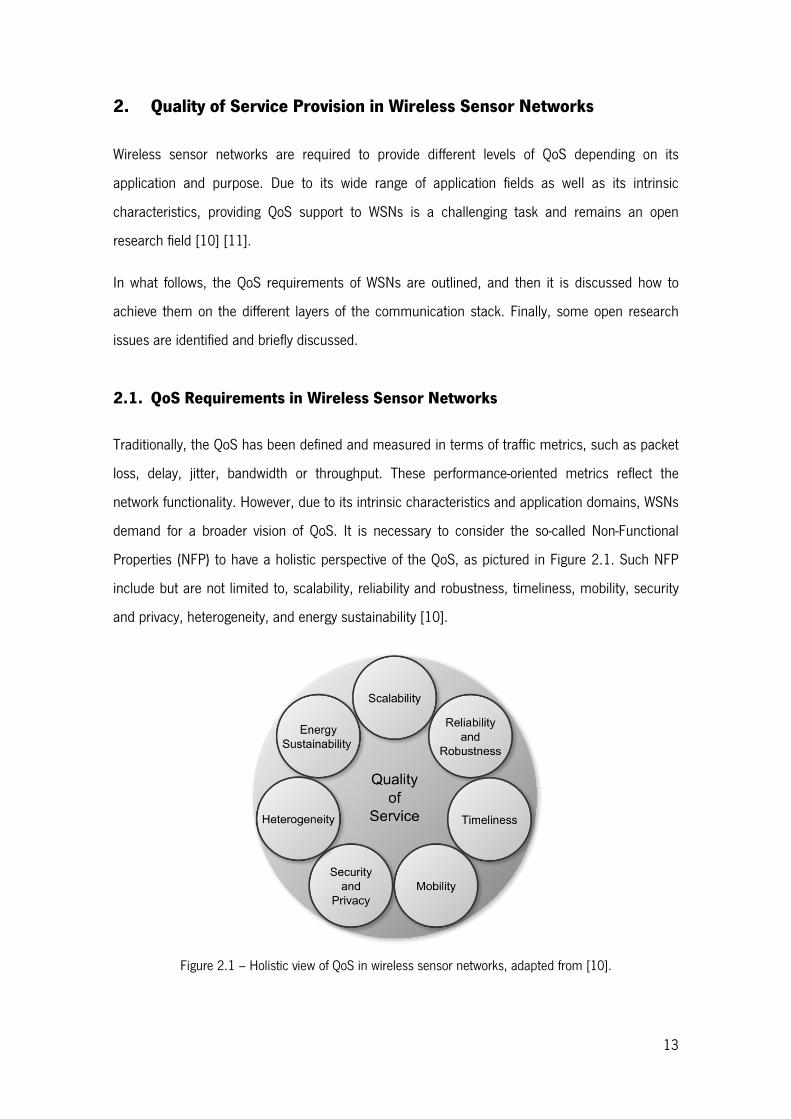
Properties (NFP) to have a holistic perspective of the QoS, as pictured in Figure 2.1. Such NFP

include but are not limited to, scalability, reliability and robustness, timeliness, mobility, security

and privacy, heterogeneity, and energy sustainability [10].

Figure 2.1 – Holistic view of QoS in wireless sensor networks, adapted from [10].

14

Depending on the WSN application and purpose, these high-level QoS requirements are then

translated into QoS metrics and/or constraints, which can be measured and evaluated.

2.1.1. Scalability

Scalability refers to the ability of a system to adapt itself in order to handle dynamic changes on

its workload in an efficient way [11]. In the context of WSNs, scalability must be seen in three

different dimensions: the network, the software, and the hardware.

Regarding the network point-of-view, a WSN can scale due to changes, in either the network

physical topology or in the network logical topology. Modifications on the physical topology may

occur because of changes in the number of nodes within the network, changes in the position of

the nodes or in its spatial density. Changes in the network logical topology can be caused by the

unreliability of the radio link quality or by the inoperability of some nodes [12] [10].

From the software perspective, scalability includes not only issues related with algorithms

efficiency and reliability (e.g., to avoid overflow of the routing tables), but also nodes

reconfiguration (e.g., to change the sampling rate) and post-deployment programming (e.g., to

add new functionalities) [13].

From the hardware side, scalability involves the ability to accommodate different sensors (e.g.,

with different interfaces) which implies the flexibility to support distinct power consumption

profiles [13].

2.1.2. Reliability and Robustness

Reliability is the ability of a system to perform as required under predefined conditions during a

specific period [14]. In addition, robustness refers to the capability of a system to perform as

required not only under its design conditions, but also under adverse circumstances unpredicted

by its designers [10] [14].

Reliability and robustness are key characteristics in the design process of WSNs regarding all its

domain of application. The network must be reliable and robust to ensure on-time data delivery

across the network despite sudden or long-term changes in the wireless channel [12]. The

software must be robust and reliable regardless of its execution conditions (e.g., algorithms must

15

operate correctly independently of the hardware in use). The hardware must be robust and

reliable even inside harsh environments (e.g., mechanical vibrations, low/high temperatures or

humidity) [10].

2.1.3. Timeliness

In general, timeliness refers to the timing behaviour of a system [10]. Depending on its

application and purpose, the timing behaviour of WSNs could be of extreme importance, not only

in terms of computations and communications, but also regarding the hardware operation (e.g.,

sensors, actuators or analogue-to-digital converters) [10].

In terms of computations, some applications (e.g., critical infrastructures monitoring or patient

monitoring), usually denoted as “real-time applications”, impose timing limitations (i.e., a

deadline) to the execution of some tasks (e.g., data aggregation or features extraction). Such

real-time applications require the use of both real-time operating system and real-time

programming languages [15].

Concerning the communications, real-time applications require on-time data delivery. In other

words, the data collected from the sensors or an event detected in a certain region must be

transmitted within a certain interval in order to be useful at the time of decision-making (e.g., in

healthcare, emergency response or fire detection systems) [16].

Another important aspect concerning the timing behaviour of WSN is related with its usability and

human interaction. WSNs are becoming increasingly pervasive and ubiquitous, enabling the

development of smart and interactive environments, plenty of sensors and actuators. In such

environments, the WSN must react on time to the human stimulus in order to provide adequate

interaction [17].

2.1.4. Mobility

Although a significant number of applications assume static WSNs, others (e.g., patient

monitoring [18] or objects tracking) must consider both physical mobility and logical mobility

[19]. Physical mobility is related with changes in the geographic location of both sensor nodes

and sink. On its turn, logical mobility refers to changes in the network logical topology. The

16

network logical topology can change due to several factors, such as: adjusts in the routing paths

in response to radio interferences, dead of some nodes due to energy depletion or changes in the

routing paths due to adding or removing nodes to/from the network. In addition, mobility can be

classified taking into account others aspects, such as the mobile entity (e.g., node mobility, sink

mobility and event mobility [20]), the mobility rate and the mobility location (i.e. intra/inter-cell

mobility) [10].

Mobility is a key requirement in WSNs since it can significantly improve the overall performance

of such networks e.g., mobility can improve the channel capacity and network scalability of WSNs

[21], mobile WSNs can reduce the energy consumption and consequently improve the network

lifetime [22]. Providing effective and efficient mobility support to WSNs is a challenging task due

to the heterogeneity of mobility sources and to the resources constrained nature of WSNs as well.

2.1.5. Security and Privacy

Considering the pervasive and critical nature of some applications supported by WSNs (e.g.,

critical infrastructures monitoring [11] or healthcare applications [9]), security and data privacy

became a key topic for their acceptance outside the labs. Indeed, in such applications, a security

breach can compromise not only the integrity of the data, but also of the physical infrastructures.

Therefore, it is vital to secure data communications within the network in order to achieve the

privacy level required by each application.

As already discussed, WSNs have very limited computational resources, memory, energy, and

bandwidth. Such limitations impose serious limitations to the degree of security that can be

applied to WSNs [23]. Moreover, by using wireless communications they are more exposed to

attacks than wired networks due to the easier access to the communication channel. To further

worsen this scenario, WSNs are wireless distributed systems without a central and trusted entity

in charge of controlling the network security and privacy [10]. Despite all these challenges, WSNs

must provide mechanisms to secure not only the network, but also the transported data, against

malicious attacks and ensure data protection and privacy.

17

2.1.6. Heterogeneity

Initial WSNs visions anticipated that sensor networks would mainly consist of homogeneous

networks [24]. However, this idea could not be further from reality. Actually, real-world WSNs

based applications are highly heterogeneous in a wide-ranging perspective and at different levels,

namely: they may use different hardware and software (e.g., sensor nodes with different

microcontrollers and radio transceivers, different network protocol implementations [25]); the

sensor nodes may be composed by different sensor types (e.g., to monitor different ambient

variables or different sensors to monitor the same variable); a WSN can be used to

simultaneously support several applications with different requirements and objectives [17].

In one word, WSNs are inherently heterogeneous. Consequently, this condition must be

considered not only at the applications design time, but also during the WSN operation, in order

to provide the QoS required by each application using the network [10].

2.1.7. Energy Sustainability

Energy is one of the scarcest resources in WSNs. Thus, energy-efficiency has been a major

research topic inside the WSNs community. As a result, several approaches have been proposed

to achieve energy efficiency and balance, and consequently increase the nodes working time,

namely, pursuing energy conservation (e.g., using data aggregation, radio duty-cycling or energy-

aware routing [26]), and energy collection (e.g., using energy harvesting) [27]. The combination

of these techniques is decisive to extend the WSNs lifetime and achieve the desired energetic

sustainability [10].

2.2. QoS Across the Communication Stack

WSNs have been used in a wide variety of areas, each of them having several target applications

with distinct QoS requirements. Therefore, the communication stack must be reliable, robust and

flexible in order to support such variety of QoS requirements. Following the internet protocol

suite, the WSNs communication stack comprises the application layer, the transport layer, the

network layer, the data-link layer and the physical layer, as shown in Figure 2.2.

18

Figure 2.2 – Typical wireless sensor networks communication stack.

In summary, the application layer depends on the WSN specific task; the transport layer ensures

efficient and reliable data delivery; the network layer is responsible for routing the data delivered

by the transport layer; the data-link layer is in charge of the medium access control and link

maintenance; and the physical layer provides robust modulation schemes and radio

management for transmitting and receiving data [1] [28]. In this way, the concerns about the

QoS provision in WSNs must be addressed at all the layers of the communication stack.

2.2.1. Application Layer

The QoS requirements of each application depend not only on its specific needs but also on its

use and purpose. First of all, during the development period, the QoS requirements of each

application must be well defined in terms of Non-Functional Properties (NFP).

2.2.1.1. Non-functional QoS requirements regarding different applications

Figure 2.3 shows some examples of WSNs applications, applied to different areas, and its QoS

requirements expressed in terms of NFP. It is important to emphasise that the set of NFP

presented in the Figure 2.3 is merely exemplificative; it is not our intention to give an exhaustive

list of NFP for each application. As a matter of example, a WSN used to carry out a patient

monitoring task must fulfil QoS requirements, such as: to deliver the data on time (timeliness), to

perform as designed (reliability) or even under adverse conditions (robustness), be used or

managed only by authorised personal (security) and protect the data of each patient (privacy).

19

Figure 2.3 – Overview of WSNs applications and some of its QoS requirements expressed in terms of NFP.

2.2.1.2. Functional QoS requirements regarding different application

Having defined the QoS requirements in terms of NFP, it is necessary to map the NFP into

functional QoS requirements (i.e., QoS metrics and/or constraints), accordingly to the

specificities of each application and the target deployment scenario, as exemplified in the Figure

2.4. Considering the aforementioned patient monitoring application, it was specified that the data

carried by the network must be delivered on time. So, such NFP must be expressed in terms of

20

end-to-end delay and packet delay variation. It was also stated that the WSN must be reliable,

which can be quantified in terms of a minimum packet reception ratio that must be

accomplished. Regarding the robustness of the WSN, it must perform as planned even when

exposed to external interferences, such as electromagnetic interferences. These electromagnetic

interferences can be reflected on the Received Signal Strength Indicator (RSSI) and on the Link

Quality Indicator (LQI). Thus, the WSN must perform as desired under a wide range of different

RSSI and LQI values. On its turn, the security and privacy mechanisms in use must take into

consideration the additional data that the network will carry (throughput) and, consequently the

necessary additional energy (energy-efficiency).

Figure 2.4 – Example of mapping NFP into functional QoS metrics and/or constraints.

21

After the specification of the QoS metrics and/or constraints in use for each application, they are

broadcasted to the lower layers of the communication stack. Then, each one of those layers is

responsible to implement the necessary mechanisms to accomplish the QoS required by each

application.

2.2.2. Transport Layer

So far as WSNs are concerned, transport protocols play a key role in achieving high levels of QoS.

Despite the many contributions to develop new transport protocols, based on distinct principles

and technical features, they all have raised concerns about the way to ensure reliable and

efficient data delivery across the network [28] [29]. Thus, NFP, such as scalability, reliability, and

timeliness, can be used to express the main design criteria and challenges related to transport

protocols. In addition, most of transport protocols implement some sort of congestion and priority

control (e.g., patient monitoring systems may require that different delivery properties should be

assigned to distinct data follows) [30].

2.2.2.1. Scalable transport protocols

WSNs may not only comprise several sensor nodes, depending on the target application and

deployment area, but also be able to admit new sensor nodes as required. Therefore, network

scalability must be addressed when designing transport protocols for WSNs. In fact, several

transport protocols prove to perform well when assessed for a large number of sensor nodes,

Table 2.1 presents some of them.

Table 2.1 – Scalable transport protocols for WSNs.

Protocol

Scalability

Number of

sensor nodes

Coverage

area (��) STCP [31] 50, 100 100 x 100

GARUDA [32] 100 650 x 650

DST [33] 200 200 x 200

ESRT [34] 200 100 x 100

TRCCIT [35] 100 60 x 60

�� [36] 200 200 x 200

ART [37] 100 300 x 300

ERTP [38] 200 180 x 180

PHTCCP [39] 100 100 x 100

CCF [40] 116 ---

22

2.2.2.2. Reliable transport protocols

Transport protocols are responsible for end-to-end connections establishment over the network

and ensure reliability regarding data delivery. Recent developments have made possible the use

of the Internet Protocol version 6 (IPv6) in low-power WSNs [41]. In particular, the practical and

efficient use of the transport protocols User Datagram Protocol (UDP) and Transmission Control

Protocol (TCP). In fact, UDP does not offer reliability or any other mechanism of control, making

it improper to many WSNs applications. On the contrary, the TCP protocol offers end-to-end

reliability; however, due to its retransmission mechanism and congestion control policy it offers

low throughput [42]. Thus, several alternative transport protocols have been proposed targeting

WSNs, along the last few years. Some of these transport protocols claim to be reliable, as

presented in Table 2.2.

Table 2.2 – Reliable transport protocols for WSNs with congestion control.

Protocol

Reliability Congestion

control Direction Level Loss recovery

STCP [31] Upstream Packet End-to-end Yes

GARUDA [32] Downstream Packet

Destination Twostage

loss recovery No

DST [33] Upstream Event End-to-end Yes

ESRT [34] Upstream Event --- Yes

TRCCIT [35] Upstream Packet Hop-by-hop Yes

CRRT [43] Upstream Packet End-to-end Hop-by-hop

Yes

CTCP [44] Upstream Packet Hop-by-hop Yes �� [36] Upstream Packet Hop-by-hop Yes

ART [37] Both Event End-to-end Yes

ERTP [38] Upstream Packet Hop-by-hop No

Reliability can be achieved in two different directions, at different levels and using distinct

methods for loss recovery. In WSNs, data transferences can occur in two directions depending on

the target application. In applications regarding the collection of sensed data, the data

transference occurs mainly in the upstream direction (i.e., from the sensor nodes to the sink).

However, in applications requiring the exchange of control messages, between the sink and the

sensor nodes, the data transference must be reliable in both directions: upstream and

downstream (i.e., from the sink to the sensor nodes). Consequently, to fulfil the reliability

23

requirements regarding data transference, the transport protocols offer upstream and

downstream reliability [29].

Moreover, reliability can be achieved at different levels. The reliability level refers to the degree of

reliability supported by the protocol. As explained in [42], three levels of reliability can be defined:

packet reliability, event reliability and destination reliability. Packet reliability refers to the

successful transfer of all the data packets. On its turn, event reliability refers to reliability of event

detection. In such cases, the protocol guarantees that at least one data packet, of each detected

event, is successfully delivered to the destination. Finally, destination reliability is related with the

ability of sending data successfully only to specific nodes.

Regarding the packet loss recovery, the methods used to retransmit the dropped packets are

hop-by-hop packet retransmission or end-to-end packet retransmission. End-to-end packet

retransmission is considered inappropriate for large-scale networks. In such cases, the packets

retransmission along multiple hops implies extra energy consumption. Hop-by-hop packets

retransmission is preferable in large-scale network as only two neighbouring nodes are involved in

the packet retransmission [29].

Additionally to these methods, some transport protocols implement a congestion control policy

(see Table 2.2) to prevent packet drops and unnecessary data retransmissions. Congestion can

occur due to different causes, such as when the combined upstream traffic exceeds the

packet-processing rate of each node or when the data throughput exceeds the link’s available

data threshold [42].

2.2.2.3. Priority-based transport protocols

Timeliness is another important requirement in WSNs. Transport protocols must not only

guarantee reliable data delivery but also provide data on time. Concerns about timeliness,

typically quantified as end-to-end delay and delay variation, must always be on top when

designing transport protocols since options related with other factors, such as reliability or

congestion control, easily affects timeliness negatively [29]. For example, the end-to-end packet

retransmission policy may introduce a significant end-to-end delay in large-scale WSNs when

compared with hop-by-hop packet retransmissions [31]. In addition, some transport protocols

implement a priority control policy, as presented in Table 2.3. Depending on the WSN

24

application, the packets carried by the network may require different delivery requirements in

terms of end-to-end delay or delay variation. Thus, introducing priority levels to differentiate data

flows, by assigning some kind of identifiers, allows each node to preferentially transmit the

packets carrying critical information. Data prioritisation is essential to support heterogeneous

applications and, consequently, data flows having different QoS requirements [29] [42].

Table 2.3 – Transport protocols classification regarding priority control.

Protocol STCP [31]

GARUDA [32]

DST [33]

ESRT [34]

TRCCIT [35]

CRRT [43]

CTCP [44]

�� [36]

ART [37]

ERTP [38]

Priority

control Yes No Yes No Yes No Yes Yes No No

The previous discussion makes it clear that several factors must be addressed to achieve high

levels of QoS when designing transport protocols targeting WSN and its huge set of target

applications. A more detailed review of such protocols can be found in [28], [29], [30] and [42].

2.2.3. Network Layer

Despite the different goals of WSNs applications, their main purpose is to sense and collect data

to be delivered to a specific destination. So, in order to deliver data efficiently, a routing protocol

is required to set up reliable and efficient multi-hop communication paths across the network

[45]. However, due to the intrinsic characteristics of WSNs, such as the random nature of the

wireless channel, the limited energy of the network nodes, and the limited computational

capabilities and memory of the network nodes, the design of reliable and efficient routing

protocols a challenging task [28].

The research and industrial communities have been proposing several routing protocols targeting

WSNs. Nevertheless, despite the different approaches, all of them share the same design goals.

Such goals, expressed in terms of NFP, include scalability, reliability and robustness, timeliness,

mobility and energy sustainability.

At the network layer, scalability means that routing protocols must be scalable enough to handle

multi-hop routes across WSNs, composed by hundreds of sensor nodes. More, routing protocols

have to deal with changes in the network topology (both, physical and logical topologies), while

choosing the best wireless links without overreacting to temporary link instability [46]. Regarding

the reliability and robustness, routing protocols must be able to select multi-hop paths that offer

25

the best performance in terms of data delivery, regardless of the wireless links instability [47].

More, real-time applications require data to be delivered on time, in order to accomplish its

requirements in terms of end-to-end delay and delay variation (i.e., timeliness) [48]. Depending

on the WSN application, mobility can be an important requirement. For example, a WSN used in

patient monitoring and tracking applications must deal with the patients’ mobility [49]. Routing in

mobile WSNs is a demanding task and, regardless of the many research efforts, several

problems are still unsolved, such as retaining the network connectivity, improving the energy

efficiency and maintaining adequate sensing coverage [22]. Another important QoS requirement

is the energy sustainability of the network. Moreover, concerns about the energy sustainability of

the WSNs must always be on top when addressing the aforementioned QoS requirements. Most

recent works on energy-aware routing protocols for WSNs agree that such protocols must be not

only energy-efficient but also improve the energy balance among the sensor nodes within the

network [26] [50].

Several methods have been proposed to achieve the aforementioned QoS requirements.

However, despite their diversity, existing WSNs routing protocols can be grouped into four main

categories, namely data-centric, hierarchical, location-based, or network flow and QoS-aware

protocols [45] [51] [46].

2.2.3.1. Data-centric routing protocols

Some WSNs applications are data-centric in the sense that they perform a task based on its

sensing activities/capabilities [52]. For example, when using a WSN designed to monitor the

temperature of industrial facilities it is impossible to ask the network where the temperature is

higher than a certain limit. In such scenario, the information source is unknown. To deal with this

problem, the research community has introduced the concept of data-centric routing. In most of

data-centric routing protocols, the data are requested to the network through queries sent to

certain regions of interest within the WSN. Then, the data are routed to their destination through

the network using distinct approaches. Table 2.4 presents a qualitative analysis of several

data-centric routing protocols considering the following aspects: energy sustainability, data

aggregation and data collection method. These aspects allow the assessment of the routing

protocols regarding their ability to fulfil some NFP, such as: energy sustainability, scalability and

timeliness.

26

Table 2.4 – Data-centric routing protocols in WSN, adapted from [46] and [45].

Protocol Energy sustainability Data aggregation Query based

SPIN [53] Weak Yes Yes F&G [54] Moderate Yes Yes DD [55] Weak Yes Yes EAR [56] Strong No Yes RR [57] Weak Yes Yes

CADR [58] Weak Yes Yes COUGAR [59] Weak Yes Yes

EAD [60] Strong Yes No GBR [61] Moderate Yes Yes

ACQUIRE [62] Moderate Yes Yes

2.2.3.2. Hierarchical routing protocols

Regarding high-density WSNs, covering large areas, single-tier networks can suffer from both lack

of scalability and data overload in some nodes. To deal with these issues, several clustering

methods have been proposed to achieve hierarchical routing. The main goal of hierarchical or

cluster-based routing protocols is to improve scalability while providing efficient multi-hop paths to

route data across the network [45]. Hierarchical routing protocols improve the network energy

sustainability by involving sensor nodes in multi-hop communications within a particular cluster

and by carrying out data aggregation and fusion, at the cluster head level, in order to minimise

the data transmitted to its destination. Hierarchical routing is a two-layer routing protocol where

the lower layer is used to select cluster heads among the sensor nodes and the higher layer is for

routing [51]. Indeed, great efforts are put into choosing the cluster heads rather than about

routing. Typically, the cluster formation is based on both the remaining energy of each node and

its proximity to the cluster head [46].

Table 2.5 presents a qualitative evaluation of most relevant hierarchical routing protocols.

Considering Table 2.5, it is possible to confirm that almost all the protocols apply data

aggregation and achieve better results, regarding the energy sustainability, when compared with

data-centric routing protocols.

27

Table 2.5 – Hierarchical routing protocols in WSN, adapted from [46] and [45].


LEACH [63] Strong Yes No SOP [64] Weak No No TEEN [65] Strong Yes No

PEGASIS [66] Strong Yes No APTEEN [67] Very Strong Yes No HEED [68] Strong Yes No

EAR-CSN [69] Strong Yes No BCEE [70] Strong Yes No

2.2.3.3. Location-based routing protocols

In some application scenarios, WSNs are randomly deployed within a region of interest to

perform location-related tasks. In such cases, it is impossible to map the sensors’ addresses with

their geographic location on the terrain. Location-based (or geographic) routing has emerged as

one of the most common routing methods regarding scenarios as the one just described. Most

location-based routing protocols make their routing decisions based on both the geographic

location of the current node and its neighbours [28], and the remaining energy of its neighbours

[71]. As presented in Table 2.6, some location-based routing protocols apply data aggregation to

improve the energy sustainability of the network. In addition to energy sustainability, the authors

of [71] use anchor nodes to minimise the routing path, and consequently the end-to-end delay

(i.e., improve the data timeliness). On its turn, the work presented in [72] shows promising

results regarding highly dynamic scenarios, including nodes with some kind of mobility.

Table 2.6 – Location-based routing protocols in WSN, adapted from [46] and [45].


GEAR [73] Moderate No No TBF [74] Moderate Yes Yes

EAGRP [75] Strong Yes No GAF [76] Weak No No

MECN [77] Weak No No SMCEN [77] Weak No No

2.2.3.4. Network flow and QoS-aware routing protocols

The routing protocols that do not fit in the previous categories are classified as network flow and

QoS-aware routing protocols [46]. In network flow protocols, the routing problem is modelled and

solved as a network flow problem [45]. On its turn, the design goals of QoS-aware routing

28

protocols are the end-to-end delay, the delay variation and energy sustainability [46] [78]. Table

2.7 shows a qualitative analysis of some network flow and QoS-aware routing protocols.

Table 2.7 – Network flow and QoS-aware routing protocols in WSN, adapted from [46] [45].


MLDG [79] Strong Yes No SAR [80] Weak Yes Yes

MLER [81] Strong No No SPEED [82] Weak No Yes

EAQSR [45] [83] Strong No Yes MCBR [84] Strong No No AODV [85] Weak No Yes

2.2.3.5. The RPL routing protocol

Among the most recently proposed routing protocols, it is possible to find the Routing Protocol for

Low-power and Lossy Networks (RPL) [86], proposed by the Internet Engineering Task Force

(IETF) working group Routing Over Low-power and Lossy Networks (ROLL). The RPL is a distance

vector routing protocol that specifies how to form a Direct Acyclic Graph (DAG) by using an

Objective Function (OF) and a set of constraints and metrics.

Several studies have been assessing the RPL performance from different perspectives. In terms

of scalability, the authors of [87] argue that RPL presents a good scalability. However, its

performance degrades when exposed to hostile environments in terms of radio interferences

which is confirmed by other works such as [88], [89] and [87]. Concerning the PRR and the

protocol overhead, the authors of [90] argue that the RPL performance is comparable to the one

achieved by the Collection Tree Protocol [91], the de-facto routing protocol in TinyOS.

Nevertheless, despite the need for more research to improve its performance, the flexibility of

RPL allows to develop application-specific OFs in order to fulfil the particular QoS requirements of

each application. Moreover, regarding its integration with existing technologies, namely IP

networks, the mechanisms introduced by RPL to perform bi-directional routing and forwarding of

IPv6 data packets allows the development of advanced monitoring applications in several

domains [89].

29

2.2.4. Data-Link Layer

The data-link layer handles the data transfer between two nodes sharing the same wireless link

[28]. Due to the intrinsic characteristics of the wireless channel, it is necessary to implement a

Medium Access Control (MAC) and a management policy in order to guarantee effective data

transfer. In this way, the MAC protocols should pursue the following key objectives defined in

terms of NFP: energy sustainability, scalability, adaptability to changes and gracefully

accommodate such network changes [92]. Other important objectives include bandwidth

efficiency, latency and throughput [28] [92]. Since many WSN applications are seen as a

collaborative effort to perform a common task, fairness is not usually considered as a key design

goal [92].

Regarding energy sustainability, MAC protocols must prevent the major energy consumption

causes, namely: collisions, overhearing, control-packet overhead, excessive retransmissions and

idle listening [28] [92]. Collisions must be avoided to prevent the retransmission of discarded

packets due to collisions. In this way, to minimise the collisions probability most MAC protocols

apply the following techniques to access the transmission medium, namely: Time Division

Multiple Access (TDMA), Carrier Sense Multiple Access with Collision Avoidance (CSMA/CA) or a

hybrid approach. Another cause of energy waste is overhearing. To prevent it, nodes must avoid

receiving data packets addressed to other nodes.

Concerning the control messages exchanged between the nodes within the network, they must

be reduced to the minimum necessary to prevent control-packet overhead and unnecessary

bandwidth utilisation. On its turn, excessive retransmissions can be caused by transmission of

data when the destination is not ready to receive it. In this way, to prevent idle listening, the

network nodes should apply a proper radio duty-cycle method to avoid listening to an idle channel

in order to receive possible traffic. It is important to notice that the use of radio duty-cycle implies

a trade-of between energy savings and end-to-end delay. While high duty-cycle methods perform

well in terms of delay, they waste more energy. On the contrary, low duty-cycle methods led to

substantial energy savings at the cost of a greater end-to-end delay. To mitigate the end-to-end

delay while preserving energy, some MAC protocols use adaptive radio duty-cycle techniques

instead of static radio duty-cycle. In static duty cycling, nodes share a timetable that is defined in

advance, and does not change according to the network traffic load. Such methods can be

suitable for applications where traffic load is known in advance, if optimised with respect to end-

30

to-end delay [93]. On the contrary, adaptive radio duty cycling methods make the radio duty-cycle

dependent of the network traffic. When compared to static duty-cycle, adaptive duty cycling MAC

protocols can reduce end-to-end delay to heavy traffic loads [93]. Table 2.8 presents a qualitative

comparison of some radio duty cycling MAC protocols.

Regarding adaptability to changes and scalability, it is important to state that such design goals

are related, as already stated when discussing scalability. Such characteristics are fundamental

to arrive at highly efficient MAC protocols that are able to optimally address the dynamics of the

network due to changes in the network size, node density, and topology. On its turn, the ability to

gracefully accommodate such network changes brings robustness to the protocol allowing it to

operate in adverse and unexpected conditions. In addition to these key requirements, MAC

protocols should implement both flow and error control mechanisms [28].

Table 2.8 – Radio duty cycling MAC protocols in WSN, adapted from [92], [93] and [94].

Protocol

Energy

sustainability Synchronization Type Duty-cycling type

S-MAC [95] Yes Yes CSMA Static WiseMAC [96] Yes No NP-CSMA Adaptive

T-MAC [97] Yes No TDMA/CSMA Adaptive DSMAC [98] Yes No CSMA/CA Adaptive

SCP-MAC [99] Yes Yes CSMA Adaptive B-MAC [100] Yes No CSMA Adaptive X-MAC [101] Yes No CSMA Adaptive

Contiki-MAC [102] Yes No CSMA/CA Adaptive

2.2.5. Physical Layer

The physical layer is in charge of frequency selection, carrier generation, signal detection,

modulation, and data encryption, providing an interface for transmitting and receiving bit streams

over the physical-communication medium [1] [28]. Due to the inherent characteristics of the

wireless channel (e.g., vulnerability to electromagnetic interferences and signal attenuation), it is

error-prone and its performance changes over time. Moreover, such weaknesses are even more

evident when harsh environments, like hospital facilities, are at stake. In this way, the physical

layer must interact with the MAC layer not only to detect and correct errors but also to share

information about the transmission conditions (e.g., transmission power, or link quality) in order

to achieve high performance while optimizing resources’ utilization [28].

31

Energy sustainability is of paramount importance for WSNs since it strongly affects the network

lifetime, as already discussed in the context of the upper layers of the communication stack.

Indeed, the energy sustainability is a cross-layer requirement that must be addressed from the

physical layer. At the physical layer, the energy is used not only by the communication module

but also by the sensors used to perform the task in which the network is participating. Regarding

the energy spent by the communication module, it has two components, namely the energy used

in operating the circuitry and the energy used to transmit/receive the bit streams [28]. While the

energy used by the circuitry is fixed (i.e., does not change along the time), the energy used to

transmit/receive data, on the contrary, varies along the time and depends on the quality of the

radio link (e.g., it depends on the channel loss, interference, transmission distance and

transmission power) [1]. In this way, it is necessary to find a trade-off between transmission

power and error-rate in order to optimize the energy consumption while achieving the highest

probability of successful data transmission [28].

Another important factor that affects the energy necessary to transmit a data stream is

modulation, as explained in [103]. Thus, regarding the communication module, the key

requirements is to include low power radio design, power-aware transmission schemes and

energy-efficient modulation schemes [1] [28] [103].

2.3. Summary

This chapter provided a broader vision about quality of service targeting wireless sensor networks

and their applications. There were presented and discussed not only several non-functional

properties, but also the main functional metrics and constrains. Finally, the key quality of service

requirements at each layer of the communication layer, and the mechanisms used to guarantee

them, were presented and discussed.

33

Chapter 3

Quality of Service Provision in BWSNs

State-of-the-art

3.1 Biomedical Wireless Sensor Networks Applications

3.1.1 At-hospital

3.1.2 At-home

3.1.3 Ambient Intelligence Systems

3.1.4 Mass Casualty Disasters

3.2 Application’s Requirements and Traffic Characterization

3.3 QoS Challenges and Open Issues in WSNs and BWSNs

3.4 Summary

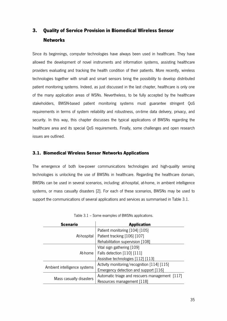
35

3. Quality of Service Provision in Biomedical Wireless Sensor

Networks

Since its beginnings, computer technologies have always been used in healthcare. They have

allowed the development of novel instruments and information systems, assisting healthcare

providers evaluating and tracking the health condition of their patients. More recently, wireless

technologies together with small and smart sensors bring the possibility to develop distributed

patient monitoring systems. Indeed, as just discussed in the last chapter, healthcare is only one

of the many application areas of WSNs. Nevertheless, to be fully accepted by the healthcare

stakeholders, BWSN-based patient monitoring systems must guarantee stringent QoS

requirements in terms of system reliability and robustness, on-time data delivery, privacy, and

security. In this way, this chapter discusses the typical applications of BWSNs regarding the

healthcare area and its special QoS requirements. Finally, some challenges and open research

issues are outlined.

3.1. Biomedical Wireless Sensor Networks Applications

The emergence of both low-power communications technologies and high-quality sensing

technologies is unlocking the use of BWSNs in healthcare. Regarding the healthcare domain,

BWSNs can be used in several scenarios, including: at-hospital, at-home, in ambient intelligence

systems, or mass casualty disasters [2]. For each of these scenarios, BWSNs may be used to

support the communications of several applications and services as summarised in Table 3.1.

Table 3.1 – Some examples of BWSNs applications.

Scenario Application

At-hospital Patient monitoring [104] [105] Patient tracking [106] [107] Rehabilitation supervision [108]

At-home Vital sign gathering [109] Falls detection [110] [111] Assistive technologies [112] [113]

Ambient intelligence systems Activity monitoring/recognition [114] [115] Emergency detection and support [116]

Mass casualty disasters Automatic triage and rescuers management [117] Resources management [118]

36

3.1.1. At-hospital

BWSNs have the potential to address some drawbacks related to wired sensing technologies

commonly used in hospitals to monitor their patients, such as reducing the number of wires

attached to patients, improving its mobility and comfort, and, at the same time, avoiding anxiety

[2].

As far as the patients’ health condition is concerned, patients’ monitoring in general or step-down

hospital units is crucial to avoid clinical worsening of patients. However, in most cases, despite

the necessity of continuous monitoring, nursing professional measures the patients’ vital or

physiological signs manually at long time intervals [104]. Such episodic measurements can be

complemented by using efficient and reliable real-time patient monitoring systems, bringing out

an enhancement of the quality of care provided, while freeing the nursing staff to provide extra

attention to the patients [105].

As surveyed in [8] and [119], several patient monitoring systems have been proposed over the

last few years. However, only a few of them were deployed in a real-world hospital environment

and evaluated by real patients. Among these are the projects presented in [104] and [105].

Chipara et al. [104], proposed a patient monitoring system to collect both the pulse rate and the

blood oxygen saturation levels. The patient monitoring system was deployed in a step-down unit

at the Barnes-Jewish Hospital in Saint Louis, MO, USA and used to monitor 41 patients for a total

of 41 days of continuous monitoring. Based on the results obtained, the authors argue that

patient monitoring system based in BWSNs are viable and achieve the same level of performance

when compared with wired monitoring system. More, this study has provided clinical examples of

early detection of clinical deterioration in patients, showing its potential to improve the quality of

care provided.

Like the previous work, MEDiSN [105] was used to monitor pulse rate and blood oxygen levels.

MEDiSN was deployed in two realistic environments, namely the University of Maryland Shock

Trauma Center and the Johns Hopkins Hospital. In the University of Maryland Shock Trauma

Center, MEDiSN was used to monitor the patients’ vital signs inside the operating room,

throughout the operation, and after the operation during their recovery period in the post

anesthesia care unit. On its turn, at the Johns Hopkins Hospital, MEDiSN was deployed within

the waiting area of the emergency room. During both deployments several problems were found,

37

such as: aluminium dividers, metallic furniture, considerable human activity, steel doors, and

lead painted walls. All these problems made the deployments challenging although, despite the

difficulties, both deployments succeed on its task. In the University of Maryland Shock Trauma

Center, MEDiSN was able to deliver, in average, 98.25 % of the sensed data, and in the

emergency room of the Johns Hopkins Hospital the data delivered was of about 95.43%, in

average. Other systems, such as those presented in [106] and [107], combine patient monitoring

with indoor localization and tracking technologies.

The LAURA project [106] is an integrated system designed to monitor the patient’s movements in

order to recognise potential harmful situations like falls or inactivity while gathering information

about the patient’s location. The movement classification engine achieves accuracy as high as

90 % when detecting dangerous situations and the localization error is lower than 2 m in 80 % of

the cases. Similarly, Cheng et al. [107] proposed a system to locate psychiatric patients while

gathering their heartbeat. In that case, the localization accuracy is 90 % with an error of about

3 m.

Another interesting application of BWSNs is related with rehabilitation supervision [108]. To

achieve optimum rehabilitation results, patients should be monitored and corrected during their

exercises. Indeed, as discussed in [108], BWSNs may radically improve the way rehabilitation is

provided, and its results evaluated.

3.1.2. At-home

National healthcare systems around the world, especially in Europe and USA, face the problem of

ageing population. This social phenomenon stresses the national healthcare systems, instigating

hospitals and medical caregivers to seek for new methods to reduce costs while maintaining the

required quality of care. Therefore, improving prevention is essential to allow people to age

actively, maintaining their quality of life. On its turn, early detection of health deterioration is vital

to help people dealing with all the diseases that arise and, at the same time, reducing the

economic and social burden of illness treatment.

BWSNs provide a valuable cost-effective communications infrastructure to develop at-home

patient monitoring applications. At-home patient monitoring applications can be used to monitor

elderly and chronically ill people, allowing automatic data collection and early detection of clinical

38

worsening. Moreover, at-home patient monitoring can improve the quality of life of chronically ill

people and reduce hospital stays. AlarmNet [109] is one example of at-home patient monitoring

system. AlarmNet was designed for long-term monitoring in ambient assisted living

environments, supporting a diverse collection of sensors and human-machine interfaces.

Keeping the discussion focused on the elderly or impaired people, falls are identified as a major

health risk. As a consequence, providing on-time care to those who fall down is of extreme

importance to minimise the risk of negative effects on people’s health. To address this problem,

several fall detection systems have been proposed. The WeCare system [110] proposes a

multi-modal fall detection system that uses sensor (e.g., body-worn accelerometers, RFID tags

and embedded video cameras) fusion technics to improve the probability to successfully detect

falls and minimise the false positives. On its turn, Castillo et al. [111], suggests a multi-modal

system that uses accelerometers, video cameras, Global Positioning System (GPS) coordinates

and machine learning techniques to detect falls and classify user’s activities in both indoor and

outdoor domestic environments.

As a consequence of aging population, the percentage of people living with any degree of

dependence, resulting from chronic diseases or any kind of physical or cognitive impairment, is

growing all around the world. In this context, several assistive technologies have been proposed.

Huo et al. [112], proposes a wireless tongue-operated assistive technology capable of detecting

the movements of the user’s tongue and translating them into commands that can be used to

control other devices in the users’ environments. Aloulou et al. [113], developed a plug-and-play

mechanism enabling the integration of several wireless assistive technologies. The development

of new assistive technologies and their integration with the users’ environment and intelligent

systems has the potential to improve the quality of life of their users [120].

3.1.3. Ambient Intelligence Systems

The problem of aging population brings new challenges to both governments and families. In

special, the demand for care at home has been increasing due to the growing number of aging

people and chronically ill people. Apart from receiving family and professional care at home,

aging and chronically ill people can benefit from technological solutions to facilitate

aging-in-place. In such context, ambient intelligence systems can support and monitor older

adults with or without any kind of physical or cognitive disease.

39

Ambient intelligence system is the vision of a technology that imperceptibly incorporates sensors,

computing devices, and information and communications technologies in our natural

environments, such as residential or nursing homes and hospitals, to support the people that

inhabiting them [121]. As described by Acampora et al. [122], ambient intelligence systems are

designed to be pervasive, ubiquitous, adaptive, transparent, personalised, context-aware and

anticipatory. Such characteristics make ambient intelligence systems appealing to develop new

healthcare systems and services [123] [124].

One of the most explored applications of ambient intelligence system is human activity

monitoring and recognition. Human activity monitoring and recognition is essential to assist aging

or disabled people on their daily life activities, or even to detect dangerous events. Amoretti et al.

[114] propose PERSONA, an activity monitoring framework for ambient assisted living

environments. PERSONA uses several data sources such as person’s posture and localisation

and the status of user-controlled devices to produce information about ongoing user activities. On

its turn, Martínez-Pérez et al. [115] proposes SCAN, an activity recognition framework to be used

in nursing homes. The SCAN framework infers the activity being made by monitoring the

behaviour of objects related to a particular activity. The authors argue that the behaviour of an

object is strongly related to a particular activity, enabling a success rate of about 92.7 % for

effective activity inference.

Hoof et al. [116] shows the results of a study performed in the Netherlands evolving the use of

ambient intelligence systems to assist older adults in their homes. The main purpose of the

ambient intelligence system used was to fire an alarm in case of emergency and study the

impact of such technology on its users. To detect such dangerous situations, the system includes

the following functionalities: mobility monitoring, voice response, fire detection, fall detection, as

well as wandering detection and prevention. Through several interviews, the authors found that

such systems increase the sense of safety and security on their users and their families.

Moreover, such technology helps to postpone the institutionalization of older adults, relieving the

pressure from the national healthcare systems.

40

3.1.4. Mass Casualty Disasters

Wireless sensor networks are self-organised, infrastructure-less and distributed networks

composed by numerous network nodes. These characteristics make WSNs suitable to be

deployed in scenarios of mass casualty events (e.g., fire-in-tunnels [125] or natural disasters

[117] [118]), providing a communications infrastructure to assist on-site emergency response.

CodeBlue [117], was one of the first projects addressing the problem of monitoring the vital

functions of a large number of patients during an emergency, improving the in-field patient triage

and tracking. Additionally, CodeBlue also provides mechanisms to locate and manage the

rescuers on the field. Similarly to CodeBlue, Chandra-Sekaran et al. [118] presents a WSN based

emergency response system designed to assist on-site organisation chief estimating and

managing its resources in order to quickly evacuate patients from the disaster site.

3.2. Application’s Requirements and Traffic Characterization

As revealed by the above discussion, BWSNs can be used in different areas and scenarios to

develop a multitude of applications. Moreover, depending on the deployment scenario, on the

application and on its use, they demand different QoS requirements. Table 3.2 shows some of

the BWSNs applications previously described and their typical QoS requirements expressed in

terms of Non-Functional Properties (NFP). See the section 2.1 of chapter 2 for more details about

the QoS requirements of WSNs.

Table 3.2 – Some BWSNs applications and typical QoS requirements expressed in terms of NFPs.

Sensor

Patient

monitoring

Patient

tracking

Rehabilitation

supervision

Falls

detection

Assistive

technologies

Scalability � �

Reliability � � � � �

Robustness � � � � �

Timeliness � � � �

Mobility � �

Security � � � � �

Privacy � � � � �

Heterogeneity � � �

Energy sustainability � � � � �

41

Depending on the BWSN application, it can be highly heterogeneous. In other words, the BWSN

can use several sensors to acquire different signals or variables as exemplified in Table 3.3. For

example, in patient monitoring applications, it is usual to have several sensors, each one

acquiring a different signal or indicator (e.g., heart rate, blood pressure, oximetry, and body

temperature).

Table 3.3 – Some BWSNs applications and typical sensors used.

Sensor

Patient

monitoring

Patient

tracking

Rehabilitation

supervision

Fall

detection

Assistive

technologies

Temperature � �

Blood pressure �

SpO2 �

Heart rate � �

Respiratory rate � �

ECG (per lead) � �

EEG (per lead) �

EMG (per lead) � �

Blood Glucose �

Accelerometer � � � �

Gyroscope � � � �

CO2 gas �

Presence � �

Video � � �

The data generated by each source (i.e., sensor or application), can vary not only in quantity but

also in form. The quantity of data generated by each source depends on the signal being

monitored (e.g., on the signal bandwidth), on the measurement resolution (i.e., the number of

samples per second) required and on the data accuracy (i.e., the number of bits per sample).

Regarding the data pattern, it may fall in one of the following categories: streaming data (i.e.,

uniform data traffic), bursty data (i.e., short bursts of data traffic) or episodic data (i.e., varying

data traffic) [126]. Table 3.4 presents the typical sensors used in BWSNs and relevant

characteristics of the data generated by each one of them.

The applications just described have the potential to improve the citizens’ quality of life in several

aspects of their daily life. However, to be an everyday reality, BWSNs must not only satisfy high

standards of QoS, but also provide easy-to-use network management tools. Network management

tools are essential to assist network administrators managing the network and supervising the

QoS provided. As a matter of example, consider a BWSN for patient monitoring purposes

42

gathering the following vital signs: temperature, heart rate and respiratory rate, and additionally

the oxygen saturation (SpO�). Looking to the Table 3.2, it is possible to see the QoS requirements of such monitoring application expressed in terms of NFP. Moreover, as discussed

in the section 2.2.1 of chapter 2, these NFP must wherever possible be quantified (e.g., the

end-to-end delay as expressed in the Table 3.4) and addressed by the different layers of the

communication stack. However, even though these QoS requirements are being addressed by

the different layers of the communication stack, they can substantially vary due to both changes

in the network topology and the environment interferences. Thus, QoS monitoring tools are

needed to monitor the real network performance and be aware of dangerous QoS degradation

situations (e.g., the end-to-end delay can be out of the limits required by each data flow).

Table 3.4 – Typical sensors used in BWSNs applications and some traffic characteristics, adapted from [126] [127] [128] [129] [130] [131].

Sensor

Maximum

data rate

Bandwidth

(Hz)

Accuracy

(bits)

Max

end-to-end

delay (s) Priority

Data

pattern

Temperature 24 bps 0–1 12 60 s Low Streaming Blood pressure 1.41 kbps 25–60 12 10 s High Bursty

SpO2 0.70 kbps 0–30 12 30 s Medium Streaming Heart rate 0.12 kbps 0.4–5 12 5 s High Streaming

Respiratory rate 0.23 kbps 0.1–10 12 5 s High Streaming ECG (per lead) 4.91 kbps 0.01–125 16 5 s High Streaming

EEG (per lead) 3.52 kbps 0.5–125 12 6 s High Streaming Episodic

EMG (per lead) 313 kbps 0–10000 16 15 s Medium Streaming Episodic

Blood Glucose 1.56 kbps 0–50 16 5 s High Streaming Episodic

Accelerometer 3.52 kbps 0–50 12 5 s High Streaming Episodic

Gyroscope 3.52 kbps 0–50 12 5 s High Streaming Episodic

CO2 gas 16 bps 0–1 8 5 s High Bursty Presence 16 bps 0–1 8 5 s Low Bursty Video 1 Mbps – – 5 s Medium Streaming

3.3. QoS Challenges and Open Issues in WSNs and BWSNs

As discussed in the chapter 2, WSNs present several challenges that are not faced by

conventional wireless networks. Such challenges bring the need for new algorithms and protocols

43

designed to meet the particular requirements of WSNs. Despite the results achieved until now,

there are several issues needing further research, namely: energy sustainability, cross-layer

solutions, suitable QoS models, hardware and software heterogeneity, cooperation, security,

mobility, interoperability, and appropriate deployment and management tools [10] [17] [132].

Most of the current work in WSNs assumes that they consist of homogeneous nodes, working

cooperatively to perform a common task. However, real deployments may consist of

heterogeneous nodes (e.g., different operating systems, different hardware platforms, and

different sensing capabilities) [101]. In such context, a WSN may be shared by several

applications, each one with its own objectives and QoS requirements (e.g., mobility, privacy, and

security). More, different WSNs may cooperate to perform a different task, to infer some results,

or to perform cooperative communications [10] [132]. Thus, there is a need for new QoS models

and communication protocols that can serve multiple applications in an efficient and reliable way

[17]. In addition, new communication protocols must facilitate the interaction with existing

networks; in other words, they must provide interoperability [10] [132].

Apart from the functional aspects and technical solutions just discussed, there is a need for new

and powerful software development tools to assist developers and architects on the development

and debugging of WSNs and their applications [133]. Moreover, more efforts are necessary to

move WSNs from labs to real-world applications. To that end, it is necessary to develop tools to

assist on the network deployment and its management during the working time [134] [133].

Network management tools are necessary not only to manage the network but also to supervise

its performance. As pointed out by the work presented in [10], the need for, not only debugging

and management tools, but also deployment planning tools was identified by the industrial end

research communities as a research goal to achieve in the medium term.

As a special set of WSNs, BWSNs share the same challenges while presenting some

particularities. As a matter of example, depending on its application and purpose, BWSNs can be

highly heterogeneous, have to support nodes mobility, have to operate in hostile environments,

have to work for long periods of time without human intervention, and at the same time providing

secure and private communications. Such QoS requirements can be achieved using the same

tools already presented for WSNs. However, in the case of BWSNs, due to the critical nature of

the data that they carry and depending on the characteristics of the deployment scenario, their

QoS requirements can be significantly harder to achieve and maintain when comparing with

44

typical WSNs. Moreover, the on-the-fly QoS provided by BWSNs must be continually monitored in

order to detect relevant and dangerous variations on it.

BWSNs designed to support patient monitoring applications inside hospital facilities have to face

several challenges, in particular, regarding the dynamic nature of the surrounding environment.

Hospital facilities can be very hostile environments for radio-frequency communications. Such

adversities result from structural factors such as the presence of metal doors and furniture, as

well as, the existence of radiation shields [2]. In fact, Ko et al. confirmed that the packet losses

for IEEE 802.15.4-based radios are higher in hospitals than in other indoor environments [135].

Moreover, IEEE 802.15.4-based networks are prone to interferences from other communication

technologies such as IEEE 802.11 (i.e., Wi-Fi networks), Bluetooth devices, and cordless phones,

all of which are habitually used in hospitals [2]. To further worsening this scenario, low-power

networks are highly vulnerable to obstacles, interferences and human bodies [2] [136]. So, in

order to address these difficulties effectively, during the applications development period, it is

necessary to develop new radio models that accurately represent hospital environments, and

integrate them with existing simulation environments.

Furthermore, from the previous discussion, it becomes clear that hospital environments could

have a significant impact on the QoS provided by BWSNs. Moreover, the dynamic of the

deployment environment affects the network performance in an unforeseeable way. The

existence of such adverse effects makes clear the necessity not only for QoS monitoring systems

but also for QoS-based network management systems.

In fact, QoS monitoring systems are essential not only to detect events able to cause degradation

on the network performance but also to provide valuable information that can be used to take

corrective measures and prevent performance degradation. On its turn, QoS-based network

management tools are needed to help “network administrators” supervising the network during

its runtime. As a matter of example, QoS-based network management is of extreme importance

to control the admission of new nodes to a BWSN. Having in mind the maximisation of the QoS

provided by a BWSN and the QoS requirements of each patient, QoS-Based admission control

tools can be used not only to assess if a new patient can be added to a BWSN but also to find the

most favourable location to place the patient.

45

3.4. Summary

This chapter discussed several aspects related with the quality of service provision in biomedical

wireless sensor networks. There were presented and discussed several applications of biomedical

wireless sensor networks targeting different scenarios. Then, the quality of service requirements

of those applications and related sensors were presented and discussed. Finally, important

quality of service challenges and open issues targeting wireless sensor networks, in general, and

biomedical wireless sensor networks, in particular, were discussed.

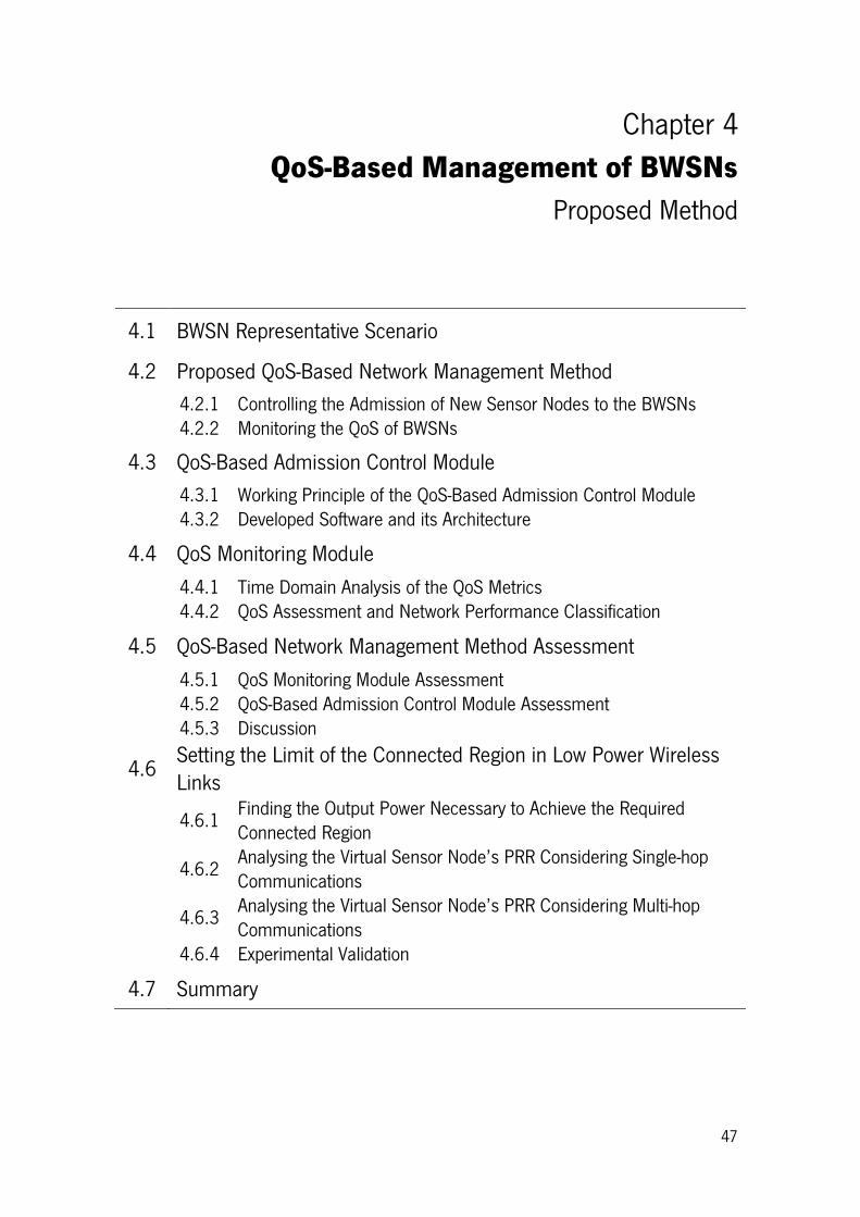
47

Chapter 4

QoS-Based Management of BWSNs

Proposed Method

4.1 BWSN Representative Scenario

4.2 Proposed QoS-Based Network Management Method

4.2.1 Controlling the Admission of New Sensor Nodes to the BWSNs 4.2.2 Monitoring the QoS of BWSNs

4.3 QoS-Based Admission Control Module

4.3.1 Working Principle of the QoS-Based Admission Control Module 4.3.2 Developed Software and its Architecture

4.4 QoS Monitoring Module

4.4.1 Time Domain Analysis of the QoS Metrics 4.4.2 QoS Assessment and Network Performance Classification

4.5 QoS-Based Network Management Method Assessment

4.5.1 QoS Monitoring Module Assessment 4.5.2 QoS-Based Admission Control Module Assessment 4.5.3 Discussion

4.6 Setting the Limit of the Connected Region in Low Power Wireless Links

4.6.1 Finding the Output Power Necessary to Achieve the Required Connected Region

4.6.2 Analysing the Virtual Sensor Node’s PRR Considering Single-hop Communications

4.6.3 Analysing the Virtual Sensor Node’s PRR Considering Multi-hop Communications

4.6.4 Experimental Validation

4.7 Summary

49

4. QoS-Based Management of Biomedical Wireless Sensor Networks

From the previous chapters it becomes clear that the use of WSN to support a wide range of

applications, each one producing distinct data with specific characteristics and QoS

requirements, brings new challenges to the WSNs research community. Consequently, the last

few years have been rich in solutions to provide the network protocol stack with mechanisms to

ensure the necessary QoS for each application or application area, as explained in the chapter 2.

Within the BWSNs context, such networks are characterised by a need for reliable and timely

data delivery. Moreover, BWSNs have to carry distinct data flows, each one with its intrinsic QoS

requirements, in a wide range of application scenarios. In addition, BWSNs should be

autonomous, scalable and operate for a long period of time without human intervention. In other

words, BWSNs must fulfil a very demanding set of QoS requirements to be fully accepted by its

users, as explained in the chapter 3.

According to the state-of-the-art, discussed in the chapters 2 and 3, the mechanisms being

proposed to provide QoS across the communication stack are of utmost importance to ensure

the required network performance. However, they do not obviate the need for a careful network

planning and management; in particular, regarding hostile real-world network deployment

environments. Indeed, QoS-based network management tools are essential, not only to monitor

the on-the-fly QoS provided by BWSNs, but also to manage the network in order to maximise the

QoS provided. Nevertheless, despite such need, the existing network planning and management

tools, targeting real-world deployments, are still quite limited in their functionality and are not

sufficiently stable, or well documented, as surveyed in [137].

In such context, this thesis proposes a new QoS-based network management method targeting

BWSNs. The proposed method aims to provide the following important and innovative

functionalities:

1 - Detect and classify QoS degradation events before the QoS reaches critical levels,

avoiding network to fail.

2 - Predict the effect, on the QoS being provided by a BWSN, of adding a new sensor node

to the network, without the need for the physical presence of the new sensor node within

the network.

50

The remaining of this chapter starts by presenting the experimental case study used to develop

the QoS-based network management method. Then, the proposed method is clearly described

and, finally, some results are presented to validate it.

4.1. BWSN Representative Scenario

The proposed QoS-based network management method was developed with the following

scenario in mind: inside a hospital or nursing home, several patients are being monitored; and

the patient monitoring system uses a BWSN to carry the data collected from each patient, as

pictured in the Figure 4.1.

Figure 4.1 – Representative scenario used to develop the proposed QoS-based network management method.

Considering the normal activity inside the representative scenario presented in the Figure 4.1, it

is necessary to guarantee that the patient monitoring system is working properly. In this way, the

network management system faces two major problems, namely:

1 - How to monitor the on-the-fly QoS provided by the BWSN and how to be aware of

potential dangerous situations regarding the network’s performance;

2 - How to choose the best location to place a new patient inside the BWSN, minimising its

impact on the QoS being provided to the patients already within the network.

51

Thus, considering the representative scenario pictured in the Figure 4.1, the proposed QoS-based

network management method must be able to assist the nursing staff facing those problems.

4.2. Proposed QoS-Based Network Management Method

With a view towards solving the problems identified in the previous section, the proposed

QoS-based network management method comprises two essential functionalities, namely the

ability to monitor the QoS effectively provided by a BWSN, and the ability to manage the

admission of new patients to a BWSN. Although such functionalities can complement each other,

they can also be used independently. For that reason, they were implemented separately.

Therefore, this thesis proposes a QoS-based network management method comprising two

modules, namely the QoS-based admission control module and the QoS monitoring module.

4.2.1. Controlling the Admission of New Sensor Nodes to the BWSN

Bearing in mind the representative scenario shown in the Figure 4.1, the QoS-based admission

control module is responsible for managing the admission of new sensor nodes (i.e., new

patients) to the BWSN. In particular, it is responsible to make a decision about the admission of

the new sensor nodes, and, for those admitted to the BWSN, find the most favourable location to

place them, while maximising the QoS provided by the BWSN.

The QoS-based admission control module starts from the premise that each sensor node, within

the BWSN, is able to simulate the presence of other sensor node on its neighbourhood. To make

this idea possible the QoS-based admission control module uses the concept of “virtual sensor

node”. In this way, every sensor node within the BWSNs must be able to create a “virtual sensor

node” and configure it, on demand, to generate data traffic as required.

Since all sensor nodes within the BWSN must be able to simulate the presence of other sensor

node on its neighbourhood, they all have to run the QoS-based admission control module.

Therefore, the QoS-based admission control must run on the sensor nodes and on the sink.

An important concern when designing the QoS-based admission control module was the

energetic sustainability of the BWSN. Thus, to avoid the problem of energy depletion in the

energy-constrained sensor nodes, due to the extra processing required, the proposed QoS-based

admission control module collects all the data required for decision making at the sink that,

52

generally, is connected to the power line. Regarding the energy consumption in the sensor nodes,

the “virtual sensor node” is required to run only on request and for short time periods, being the

extra energy consumption insignificant.

Another important requirement when designing the QoS-based admission control module was its

portability among different operation systems (e.g., the Contiki OS or the Tiny OS) and compilers.

In this way, to maximise the module portability it was implemented using ANCI C. Moreover, the

modules’ architecture was designed for easier integration with other WSN applications.

4.2.2. Monitoring the QoS of BWSNs

Once again, considering the representative scenario pictured in the Figure 4.1, the QoS

monitoring module is in charge of monitoring the QoS provided by the BWSN. In order to do so,

the QoS monitoring module must be able to assess each data flow carried by the network, and to

detect potential QoS degradation events. The QoS monitoring module detects the potential QoS

degradation events by analysing the behaviour of each one of the metrics used to quantify the

QoS provided by the network (n.b., the most common metrics used to quantify the QoS provided

by WSNs and BWSNs were presented in the chapter 2 and 3, respectively). Moreover, the QoS

monitoring module classifies the QoS degradation events detected in order to provide extra

information concerning the potential risk that each detected event represents to the QoS being

provided by the BWSN.

As the QoS monitoring module must assess each data flow carried by the BWSN, it must run on

the sink or on the computer connecting the BWSN to the outside world (e.g., the computer

interfacing the BWSN with the healthcare information system as pictured in the Figure 4.1), in

order to perform efficiently. In the context of this thesis, the QoS monitoring module was put into

operation in the computer connected to the sink node.

To install the QoS monitoring module into the computer that connects the BWSN to the hospital

information system brings some important advantages. The most important one is the

independence of the QoS monitoring module with respect to the BWSN. By using this

architecture, the QoS monitoring module and the BWSN must agree only on the format of the

messages exchanged within the networks. Other important advantages relate to the larger

processing power and memory available when comparing the computer with the BWSN nodes.

53

Finally, the use of the computer facilitates the interoperability of the QoS monitoring module with

other information systems.

4.3. QoS-Based Admission Control Module

The QoS-based admission control module uses a probe-based admission control procedure to

decide where a new sensor node can join the network. The decision regarding where to admit the

new sensor node on the network is based on time-domain analysis of the performance metrics

used to quantify the QoS provided by the network, namely the packet reception ratio. Within the

proposed method, the probe-based procedure of the QoS-based admission control module uses a

“virtual sensor node” called QoS Probe to mimic the presence of a new real sensor node on its

neighbourhood, when necessary (e.g., on-demand or periodically triggered by software). The use

of a “virtual sensor node” avoids the necessity of the new sensor node to be physically present

within the network and enables to assess the network performance from a remote location, in

order to decide about the best location to admit the new sensor node within the network.

4.3.1. Working Principle of the QoS-Based Admission Control Module

Traditional admission control systems use a signalling protocol to establish bandwidth

reservations at all routers along the data path. This approach has to preserve per-flow state and

to process per-flow reservation messages at all routers, resulting in limited scalability and high

computational complexity. To avoid those problems, the proposed admission control method

follows the endpoint admission control approach in the sense that the admission test is made at

the edge nodes, and it is made for the entire path from the source to the sink node [138] [139].

In this way, the proposed admission control method avoids the complexity of per-hop schemes

without adding any complexity to the network nodes. The admission control is done through a

“virtual sensor node” on the network, to mimic the presence of the new real node on its vicinity,

and measuring how it affects the QoS provided by the network.

The admission procedure, which is controlled by the network administrator (or who is in charge,

hereinafter referred as operator), has the following phases: first the operator selects the type of

sensor node to be added to the network and its preferential location in the network; then the

operator requests the system to evaluate the network in order to assess its QoS; finally, based on

the information retrieved by the system, the operator decides where the node can be admitted to

54

the network. During the network evaluation phase, the system configures the QoS Probe, running

on one of the sensor nodes placed in the location chosen to add the new sensor node, to mimic

the presence of the new sensor node. Then, the QoS Probe starts sending a data flow, identical

to that which will be generated by the real node, to the sink. Finally, the system analyses the

changes in the network’s QoS introduced by the new data flow and reports it to the operator that

decides where the new sensor node can be admitted to the network. Figure 4.2 shows the

probing procedure and all the messages exchanged to assess if the new sensor node can be

admitted to the network.

Figure 4.2 – The probing procedure performed to verify if a new node can be admitted by the network.

4.3.2. Developed Software and its Architecture

The software developed to implement the proposed QoS-based network management method,

and to run on each node within the BWSN, was built on top of the Contiki OS [140] and follows

the architecture presented in the Figure 4.3. The software developed interacts with the Contiki

55

OS at two levels, namely at the application layer and at the network layer. This architecture

facilitates the software portability to other operating systems or to be used with other

communication stacks.

Figure 4.3 – Architecture of the software running on the BWSN’s nodes.

The software developed to implement the QoS-based network management method adds the

following modules to the base operating system architecture: QoS Manager, QoS Profile, QoS

Probe, QoS Analyser and QoS Daemon. The QoS Manager is the interface between the

application and the QoS-based network management software. It is responsible to manage the

interactions between all the remaining components. The application uses the QoS Manager to

receive information about the QoS provided by the network or to trigger actions, such as the

admission control procedure. The QoS Profile contains all the relevant information about each

data flow including the required QoS. The QoS Probe (i.e., the “virtual sensor node”) runs only on

the sensor nodes. It can be configured, on demand, to perform remote tasks. Such tasks include

generating specific data flows or collecting information about the node performance (e.g., its

radio link quality). The QoS Analyser runs only in the sink node and extracts the relevant

information about each data flow to assess the real-time QoS provided by the network and, if

necessary, generates alerts to the healthcare information system. Finally, the QoS Daemon is in

charge of all the control and signalling communications between the nodes within the BWSN.

4.4. QoS Monitoring Module

The QoS monitoring module collects relevant information about the network’s performance and

uses it to detect and classify QoS degradation events. Based on this information, reports are

generated to inform the network administrator, or who is in-charge, about the network’s

performance.

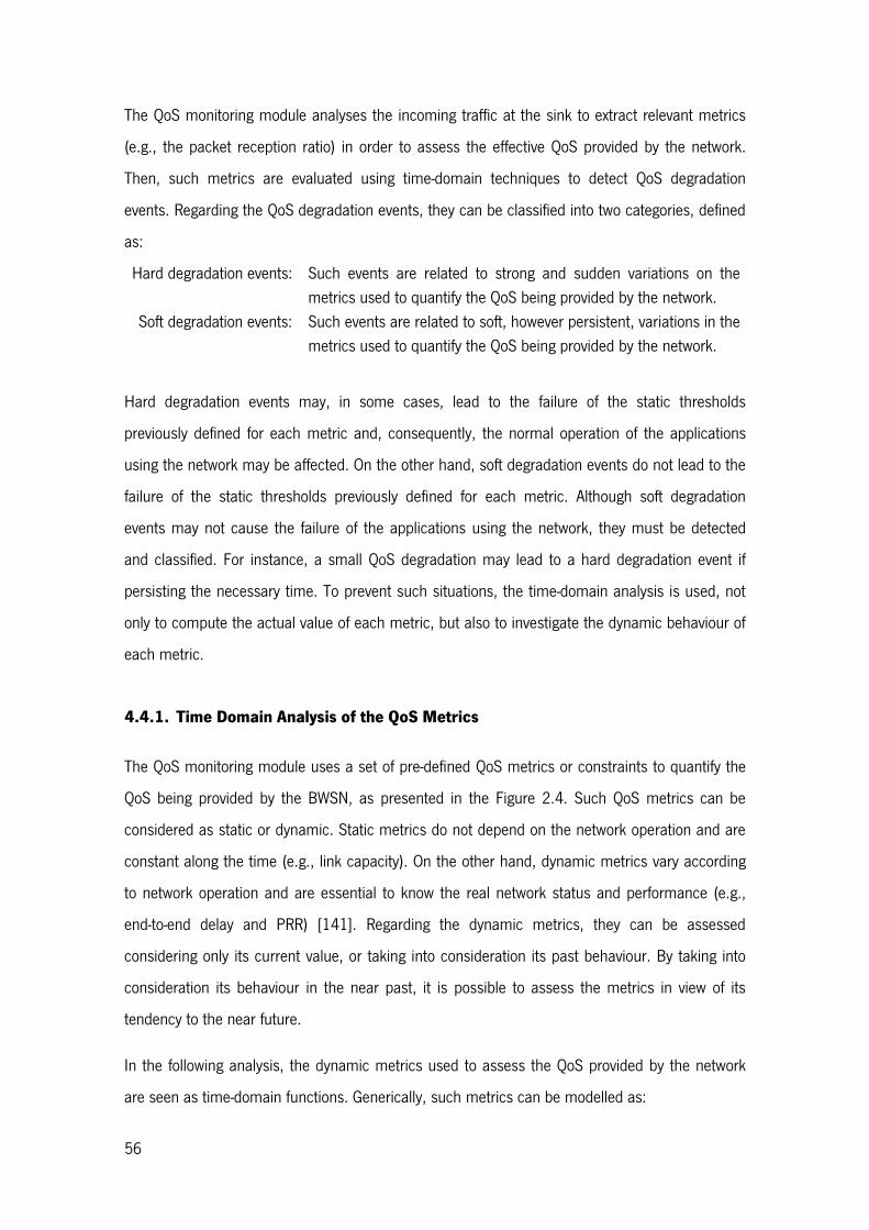
56

The QoS monitoring module analyses the incoming traffic at the sink to extract relevant metrics

(e.g., the packet reception ratio) in order to assess the effective QoS provided by the network.

Then, such metrics are evaluated using time-domain techniques to detect QoS degradation

events. Regarding the QoS degradation events, they can be classified into two categories, defined

as:

Hard degradation events: Such events are related to strong and sudden variations on the

metrics used to quantify the QoS being provided by the network.

Soft degradation events: Such events are related to soft, however persistent, variations in the

metrics used to quantify the QoS being provided by the network.

Hard degradation events may, in some cases, lead to the failure of the static thresholds

previously defined for each metric and, consequently, the normal operation of the applications

using the network may be affected. On the other hand, soft degradation events do not lead to the

failure of the static thresholds previously defined for each metric. Although soft degradation

events may not cause the failure of the applications using the network, they must be detected

and classified. For instance, a small QoS degradation may lead to a hard degradation event if

persisting the necessary time. To prevent such situations, the time-domain analysis is used, not

only to compute the actual value of each metric, but also to investigate the dynamic behaviour of

each metric.

4.4.1. Time Domain Analysis of the QoS Metrics

The QoS monitoring module uses a set of pre-defined QoS metrics or constraints to quantify the

QoS being provided by the BWSN, as presented in the Figure 2.4. Such QoS metrics can be

considered as static or dynamic. Static metrics do not depend on the network operation and are

constant along the time (e.g., link capacity). On the other hand, dynamic metrics vary according

to network operation and are essential to know the real network status and performance (e.g.,

end-to-end delay and PRR) [141]. Regarding the dynamic metrics, they can be assessed

considering only its current value, or taking into consideration its past behaviour. By taking into

consideration its behaviour in the near past, it is possible to assess the metrics in view of its

tendency to the near future.

In the following analysis, the dynamic metrics used to assess the QoS provided by the network

are seen as time-domain functions. Generically, such metrics can be modelled as:

57

�"#$ = �∗"#$ + ()�"#$, with# ≥ 0, Eq. 4.1

where �"#$ represents the measured value of the metric, �∗"#$ represents the real value of the metric, and the white Gaussian noise function ()�"#$ represents the metric’s variation due to random interferences and the natural fluctuations of the network.

4.4.1.1. Computing the metrics value

After the setup time, a network tends to be stable and the metrics used to compute the network’s

QoS can be found stable, despite the small fluctuations that can be observed. Thus, a moving

average filter can be used to estimate the value of the metrics used to quantify the QoS provided

by the network, cancelling the effect of such small fluctuations. Therefore, consider the following

moving average filter:

/"),�, �$ = 101)"� − �$,234

567 Eq. 4.2

where )"∙$ represents the signal to be filtered, � is the number of observations used in the

moving average, � is the index of the most recent observation of the sample to be processed, and 0 = � if � < � or 0 = � in other cases. The use of moving average filters reduces the effects of random instabilities on the metric. Thus, the estimated value of the metric is

represented by �:"�$, and its value is computed as: �:"�$ = /"�,�, �$. Eq. 4.3

The number of observations used to estimate the value of each metric depends both on the

network operation and on the deployment environment. As a matter of example, consider a

network deployed inside a hostile environment in which the quality of the wireless links can often

vary considerably. In such case it is reasonable to use a large number of observations to estimate

the metric’s value; in other words, it is necessary to analyse the network during the last � seconds, being � the time necessary to compute the metric’s observations being considered. Therefore, the value of � must be determined taking into consideration the network typical

operation and the target deployment environment.

58

4.4.1.2. Detecting major variations in the metrics value

The network operation can be affected by both external events (e.g., radio interferences) and

internal events (e.g., node dead due to energy depletion). In both circumstances, these events

may reflect itself as perturbations in the metrics being used to assess the network’s QoS.

Detecting such perturbations is of major importance to prevent the degradation of the network’s

performance.

In such context, the dynamic of the metric is signified by its first derivative and represented by

�:< "�$. Therefore, we propose the use of two features to detect major perturbations in the metric’s value, namely the energy of �:< "�$:

=>:< "�$ = 1?�:< "� − �$?�,234

567 Eq. 4.4

and an energy threshold dynamically computed as:

=@ABCDAEFG"�$ = /H=>:< , �, �I. Eq. 4.5

The perturbations potentially harmful to the network’s performance are detected by comparing

the actual E>:< against the EKLMNOLPQR. Thus, a potential harmful perturbation is detected if the actual energy of the metric differentiation is greater than the energy threshold, E>:< > EKLMNOLPQR. In order to quantify the potential degradation caused by harmful perturbations, a Metric

Degradation Index (MDI) was defined as:

TUV = W=>:< /=@ABCDAEFGY. Eq. 4.6

The TUV gives quantitative information about the change on the metric energy. After calibration, the TUV can be used to detect potential degradation events. The higher the TUV, the greater is the potential degradation of the network performance. To calibrate the TUV, several approaches can be used, depending on the QoS monitoring strategy. One possibility

consists of using the maximum TUV achieved during the normal network operation as a threshold to detect degradation events and fire alert messages. Other possibility is using the

TUV’[ mean value achieved during the network normal operation.

59

4.4.1.3. Detecting small variations in the metrics value

Although useful to detect significant perturbations on the metrics being analysed, the previous

analysis is insensitive to small and monotonic metrics variations. In other words, the previous

analysis is insensitive to variations resulting in =>:< ≤ =@ABCDAEFG. To detect such small variations three figures-of-merit are used, namely: the Metric Tendency (MT), the Zero-Crossing-Rate (ZCR),

and the classification of the most recent observation of the metric as a Single Global Minimum

(MIN) or a Single Global Maximum (MAX) within the sample being processed.

Let’s consider the functionsℎ] , � = 1,… , _. The product function of these functions h` is represented by ℎ4 ∙ ℎ� ∙ … ∙ ℎa"∙$ = ∏ ℎ5a564 "∙$. In the case of ℎ4 ≡ ℎ� ≡ ⋯ ≡ ℎa ≡ ℎ, we obtain ℎa"∙$ = ∏ ℎa564 "∙$. By �� we denote the identity function. The MT can be determined looking to the Slope (S) of a linear regression curve obtained using

the method of the least squares, as:

�>: "�$ = /"�� ∙ �:,�, �$ − /"��, �, �$/"�:,�, �$/"��, �, �$ − /�"��, �, �$ . Eq. 4.7

Within the sample being processed, if �>: < 0 the T�>: is to decrease (↓), if �>: > 0 the T�>: is to increase (↑) and, finally, if �>: = 0 the T�>: is to be constant (→).

On its turn, the ZCR feature is defined as:

hi�>:< "�$ = 1201 j[)� k�:< "� − �$l − [)� k�:< "� − 1 − �$lj234

567, Eq. 4.8

where [)� is the sign function. Finally, to verify if the observation �:"�$ is a single global minimum or a single global maximum, within the sample being processed, the following expressions are used, respectively:

TV�>: "�$ = m1,�:"�$ > �:"�$, ∀� ∈ p� − 0 + 1, � − 1q0, ��r#ℎstu�[s[ , Eq. 4.9

and

Tvw>: "�$ = m1,�:"�$ < �:"�$, ∀� ∈ p� − 0 + 1, � − 1q0, ��r#ℎstu�[s[ . Eq. 4.10

60

The filter’s order (i.e., the length of the sample being processed) used to compute the previous

figures-of-merit depend on the QoS monitoring policy in use. Considering a small value of �, the

QoS monitoring system becomes very sensitive and reactive. In opposition, a QoS monitoring

system less reactive must use a higher � value. Nevertheless, it is necessary to find equilibrium

between the filter’s order and the desired reactiveness of the QoS monitoring system.

By using these three figures-of-merit it is possible to detect small and monotonic variations, over

the sample being processed, on the metric being analysed. By detecting such situations,

corrective measures can be taken to prevent the further degradation of the QoS provided by the

network.

4.4.2. QoS Assessment and Network Performance Classification

Considering the classification presented in [142], the QoS metrics used to assess the network’s

performance can be sorted into two sets: those that need to be maximised, denoted as �>xy and, the remaining that need to be minimised�>5z. Based on this classification, and using the features previously presented, it is possible to analyse the performance of the network and

classify suspicious events.

The network performance assessment and classification if the QoS metric belongs to �>xy, is analysed using the criteria presented in the Table 4.1, resulting in the following rule to detect

Performance Degradation (PD):

�U>xy = H�:< < 0��=>:< > =@ABCDAEFGIrt p"�:< < 0��>: < 0$��"hi�>:< = 0rtTV�>: = 1$q Eq. 4.11

Table 4.1 – Network performance assessment and classification if QoS metric belongs to �>xy. �:< {�:< |}�: ~��:< |��: Network performance Example < 0 ≤ =@ABCDAEFG ↓ > 0 1 degrading Figure 4.4 a) < 0 ≤ =@ABCDAEFG ↓ > 0 0 not degrading or recovering Figure 4.4 b) < 0 ≤ =@ABCDAEFG ↓ = 0 n.a. degrading Figure 4.4 c) < 0 ≤ =@ABCDAEFG → rt ↑ n.a. n.a. not degrading Figure 4.4 d) < 0 > =@ABCDAEFG n.a. n.a. n.a. degrading Figure 4.4 e) ≥ 0 n.a. n.a. n.a. n.a. not degrading Figure 4.4 f)

Figure 4.4 shows typical patterns detected using the rules presented in the Table 4.1. By using

those rules, QoS degradation is detected when the patterns of figures Figure 4.4 a), c) and e)

61

appear. On the contrary, the patterns of Figure 4.4 b), d) and f) indicate that the network is

working as required; therefore no QoS degradation is detected. As a matter of example, consider

the patterns presented in the Figure 4.4 a) and b), in both cases the metric is slightly fluctuating

and decreasing (i.e., the metric tendency (MT) is to decrease and the ZCR is greater than zero).

The difference between those two patterns is detected by looking to the value of the metric at the

time that the metric is being assessed (i.e., at # = �). In the case of the Figure 4.4 a), the value of the metric is a global minimum and the metric is considered to be degrading. On the contrary,

in the case of the Figure 4.4 b), the value of the metric is not a global minimum and the metric is

considered to be recovering from a short-time and negligible diminution of its value.

Figure 4.4 – Some examples of patterns detected using the rules presented in the Table 4.1.

On the other hand, if the QoS metric belongs to m��, the rule to detect PD, derived from Table 4.2, is:

�U>5z = H�:< > 0��=>:< > =@ABCDAEFGIrt p"�:< > 0��>: > 0$��"hi�>:< = 0rtTvw>: = 1$q Eq. 4.12

Table 4.2 – Network performance assessment and classification if QoS metric belongs to �>5z. �:< {�:< |}�: ~��:< |��: Network performance Example > 0 ≤ =@ABCDAEFG ↑ > 0 1 degrading Figure 4.5 a) > 0 ≤ =@ABCDAEFG ↑ > 0 0 not degrading or recovering Figure 4.5 b) > 0 ≤ =@ABCDAEFG ↑ = 0 n.a. degrading Figure 4.5 c) > 0 ≤ =@ABCDAEFG → rt ↓ n.a. n.a. not degrading Figure 4.5 d) > 0 > =@ABCDAEFG n.a. n.a. n.a. degrading Figure 4.5 e) ≤ 0 n.a. n.a. n.a. n.a. not degrading Figure 4.5 f)

62

Figure 4.5 shows representative patterns detected using the rules presented in the Table 4.2.

Using those rules it is possible to detect QoS degradation when the patterns of figures Figure 4.4

a), c) and e) appear. On the contrary, the patterns of Figure 4.4 b), d) and f) indicate that the

network is working well; therefore no QoS degradation is observed. As a matter of example,

consider the patterns presented in the Figure 4.5 a) and b), in both cases the metric is slightly

fluctuating and increasing (i.e., the metric tendency (MT) is to increase and the ZCR is greater

than zero). The difference between those two patterns is detected by looking to the value of the

metric at the time that the metric is being analysed (i.e., at # = �). In the case of the Figure 4.5 a), the value of the metric is a global maximum and the metric is considered to be degrading. On

the contrary, in the case of the Figure 4.5 b), the value of the metric is not a global maximum

and the metric is considered to be recovering from a short-time and negligible growth of its value.

Figure 4.5 – Some examples of patterns detected using the rules presented in the Table 4.2.

By using the rules presented in the Table 4.1 and Table 4.2, it is possible to detect and classify

potential QoS degradation events. Consequently, this information can be used to inform the

network administrator to take measures to mitigate the degradation of the network performance.

4.5. QoS-Based Network Management Method Assessment

To assess the suggested QoS-based network management method, a case study considering a

typical BWSN was simulated. Network simulators are widely used to evaluate and compare the

performance of WSNs. Their use has advantages and disadvantages. Despite they are an

63

approximation to the reality (e.g., by using oversimplified channel models), they allow easy and

network deployments, controllable and flexible scenarios and the repeatability of the results

obtained. On the other hand, real-world deployments avoid problems relating to simplification of

models, but such network deployments are more expensive and considerably harder to

implement and deploy. However, despite its complexity, real-word deployments represent a great

driving force in order to ensure the users’ acceptance of WSN in general and of BWSNs in

particular.

Bearing in mind the above, the proposed QoS-based network management method was tested

taking advantage of these two realities. The simulated environment was used during the

development stage to rapidly assess the method and make adjustments whenever required. The

simulated environment was based on the cross layer emulation and simulation tool known as

COOJA [143]. COOJA is a flexible WSNs hardware emulator and network simulator designed to

simulate WSNs running the Contiki OS [140].

Figure 4.6 – Network deployment. The sensor nodes are regularly distributed over an 80 m x 80 m area. Each node has a radio range of 30 m. The sink is at position (40, 40).

Facing the impossibility to simulate all the possible situations regarding a patient monitoring

system deployed in a real hospital environment, the scenario presented in the Figure 4.6 was

envisioned to assess the proposed QoS-based network management method. Such scenario aims

to recreate the spatial location of 24 patients being monitored within a hospital floor. In such

context, to maximise the covered area and, at the same time, minimise the probability of

collisions and the effect of funnelling to the sink, the BWSN was regularly deployed in a square

area [144], as pictured in the Figure 4.6.

The 25 nodes (i.e., 1 sink and 24 sensor nodes, one for each patient) have a radio range of

30 m and, after the network setup time, which is of about 60 s, each sensor node starts sending

64

data packets at a specific rate. See Table 4.3 for a detailed description of both the network and

the simulation configurations.

Table 4.3 – Network, application, and simulation configurations.

Network:

Deployment Area (m) 80 x 80

Deployment Type 5 x 5 grid (see Figure 4.6)

Number of Nodes 1 sink and 24 sensor nodes

Sink Position (m) (40, 40)

Radio Range (m) 30

Radio Model Unit Disk Graph Medium Distance Loss

Network Layer IPv6 with 6LowPAN

Transport Layer User Datagram Protocol (UDP) [145]

Routing Protocol RPL with the MRHOF [146]

Logical Topology Random PRR Required 98%, 91%

Application:

Task Type Time driven

Data Length (byte) < 70 (one packet) Reporting Interval (s) 1, 2

Simulation:

Time (s) 1000

To evaluate the proposed QoS-based network management method, several simulations were

made and the corresponding results analysed. The evaluation consists of two parts. First, the

QoS monitoring module is used to detect and classify potential harmful events relating to QoS

degradation. Then, the admission control module is used to verify if a new sensor node can be

admitted by the network in the requested area. In both scenarios the PRR is taken as a

figure-of-merit to evaluate the QoS provided by the network. The PRR was defined as:

�� = 4�∑ ��

�564 , Eq. 4.13

where T is the number of sensor nodes on the network, �5 is the number of data packets received by the sink from the sensor node �, and �5 is the number of data packets sent by the sensor node �.

4.5.1. QoS Monitoring Module Assessment

Regarding the QoS monitoring module, it was tested in order to evaluate its capacity to detect not

only small and monotonic variations in the PRR (i.e., the metric being used to assess the QoS

65

provided by the network), able to cause QoS degradation in the long term, but also sudden

variations in the PRR potentially dangerous for QoS.

Figure 4.7 shows the PRR and its first derivative when the network was running on its normal

operation. When comparing the Figure 4.7 with the Figure 4.8 it was possible to verify that, by

using the features and rules of the Table 4.1, the QoS monitoring module is able to detect and

classify different suspicious events related to the QoS degradation.

Figure 4.7 – PRR of the network in its normal operation. The PRR dynamics is represented with its first derivative.

A detailed observation of Figure 4.8 permits to verify (around 440 s and 490 s) that using both

information about the PRR dynamics and the previous defined figures-of-merit (i.e., the

figures-of-merit defined in the Table 4.1), the QoS monitoring module was able to detect slight

and monotonic variations in the PRR. Moreover, if we look carefully to the PRR presented in the

Figure 4.7 and compare its shape with the patterns presented in the Figure 4.4, it is possible to

verify that the QoS degradation events are detected when the patterns shown in Figure 4.4 a) and

c) are detected. Concerning the detection and classification of potentially harmful QoS

degradation events using the energy feature (i.e., by detecting the pattern presented in the Figure

4.4 e)), it is important to notice that small values of the MDI correspond to small variations on

the metric being analysed.

66

To verify how the QoS monitoring module responds to external interferences, such as radio

interferences or link degradation, variations were introduced on the Unit Disk Graph Medium

Distance Loss (UDGM-DL) radio model, used within the COOJA simulator. The UDGM-DL is a

wireless channel model where the transmission range is modelled as an ideal disk. The sensor

nodes outside this disk don’t receive packets. The sensor nodes inside the disk receive packets

accordingly a probability that depends on several parameters, according to the following

equation: � = �� − ��"��/�>xy� $"1 − ��$, where �� represents the probability of a node to successfully transmit a packet, the �� is the probability of a node to successfully receive a packet, � is the distance between the two sensor nodes, and �>xy is the maximum transmission range. The external interferences were simulated by changing the �� and �� probabilities of the UDGM-DL radio model as shown in the Table 4.4.

Figure 4.8 – PRR energy and its dynamic threshold. It is possible to see the QoS degradation alerts and it’s MDI.

Table 4.4 – UDGM-DL radio model used to simulate radio interferences, see Figure 4.9.

Simulation time on the Figure 4.9 (s) 0 400 500 600 700 800 900

Tx and Rx success ratio (%) 100 75 100 50 75 80 100

In order to introduce selectivity on the detection of significant degradation events, and at the

same time avoid alarm fatigue due to over-alarming, a threshold was introduced in the MDI. In

this way, the maximum MDI value obtained during the normal network operation (i.e., MDI = 4)

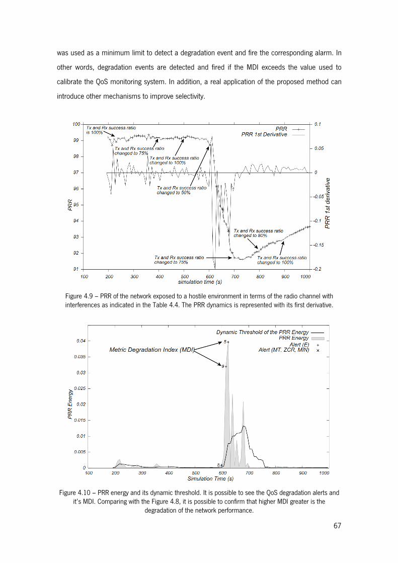
67

was used as a minimum limit to detect a degradation event and fire the corresponding alarm. In

other words, degradation events are detected and fired if the MDI exceeds the value used to

calibrate the QoS monitoring system. In addition, a real application of the proposed method can

introduce other mechanisms to improve selectivity.

Figure 4.9 – PRR of the network exposed to a hostile environment in terms of the radio channel with interferences as indicated in the Table 4.4. The PRR dynamics is represented with its first derivative.

Figure 4.10 – PRR energy and its dynamic threshold. It is possible to see the QoS degradation alerts and it’s MDI. Comparing with the Figure 4.8, it is possible to confirm that higher MDI greater is the

degradation of the network performance.

68

The Figure 4.9 shows that the radio interferences introduced in the simulation produced a strong

degradation in the PRR and consequently in the QoS provided by the network. Analysing the

Figure 4.9, and comparing it with the Figure 4.10, it is possible to confirm that the QoS

monitoring module detected the QoS degradation at its very beginning. More, from these results

it is possible to confirm that high values of the MDI suggest that the metric being analysed will

suffer a strong degradation. Comparing the Figure 4.8 (i.e., the network normal operation) with

the Figure 4.10 (i.e., the network suffering a strong perturbation), it is possible to confirm that

the higher MDI the greater is the degradation of the network performance.

By detecting the QoS degradation events at its beginning, the QoS monitoring module can also be

used to fire messages informing the network manager about the possible QoS degradation. On its

turn, the network manager can take measures to mitigate the effects of the QoS degradation

even before it takes critical values.

In addition to the present analysis, the proposed method can be used to assess the performance

of each individual node within the network. This possibility, while requiring additional

computational power and memory, allows obtaining additional information about the network

performance. In particular, monitoring individual nodes is crucial to identify the source of the

performance degradation events, which is impossible when analysing the overall performance of

the network.

4.5.2. QoS-Based Admission Control Module Assessment

To test the admission control module, the aforementioned probing procedure was used to

evaluate if a new sensor node can be admitted to the network in the place under test. The

probing procedure starts on request (e.g., by a healthcare professional) and stops when one of

the following conditions is observed: the metric value crosses a pre-established limit or the metric

tendency (to increase or decrease) is interrupted, in other words �>: ≥ 0 for the metrics belonging to �>xy, and �>: ≤ 0 for the metrics belonging to �>5z. Nevertheless, if none of these conditions occur, the probing procedure ends after a pre-established timeout.

Regarding the evaluation of the admission control module, two scenarios were considered. For

the first, each sensor node within the network was set to generate constant bit rate traffic of

about 0.5 packets per second, where the network is considered uncongested and able to admit a

new sensor node while maintaining a PRR of, at least, 98%. In the second scenario, the sensor

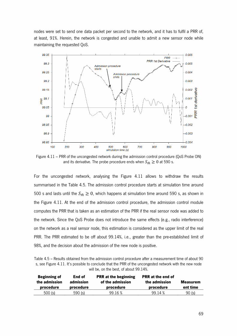
69

nodes were set to send one data packet per second to the network, and it has to fulfil a PRR of,

at least, 91%. Herein, the network is congested and unable to admit a new sensor node while

maintaining the requested QoS.

Figure 4.11 – PRR of the uncongested network during the admission control procedure (QoS Probe ON)

and its derivative. The probe procedure ends when �>: ≥ 0 at 590 s.

For the uncongested network, analysing the Figure 4.11 allows to withdraw the results

summarised in the Table 4.5. The admission control procedure starts at simulation time around

500 s and lasts until the �>: ≥ 0, which happens at simulation time around 590 s, as shown in the Figure 4.11. At the end of the admission control procedure, the admission control module

computes the PRR that is taken as an estimation of the PRR if the real sensor node was added to

the network. Since the QoS Probe does not introduce the same effects (e.g., radio interference)

on the network as a real sensor node, this estimation is considered as the upper limit of the real

PRR. The PRR estimated to be off about 99.14%, i.e., greater than the pre-established limit of

98%, and the decision about the admission of the new node is positive.

Table 4.5 – Results obtained from the admission control procedure after a measurement time of about 90 s, see Figure 4.11. It’s possible to conclude that the PRR of the uncongested network with the new node

will be, on the best, of about 99.14%.

Beginning of

the admission

procedure

End of

admission

procedure

PRR at the beginning

of the admission

procedure

PRR at the end of

the admission

procedure

Measurem

ent time

500 (s) 590 (s) 99.16 % 99.14 % 90 (s)

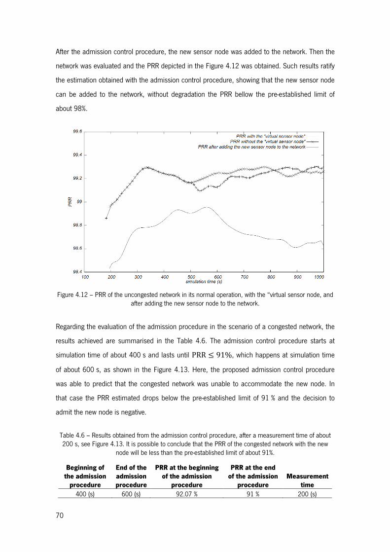
70

After the admission control procedure, the new sensor node was added to the network. Then the

network was evaluated and the PRR depicted in the Figure 4.12 was obtained. Such results ratify

the estimation obtained with the admission control procedure, showing that the new sensor node

can be added to the network, without degradation the PRR bellow the pre-established limit of

about 98%.

Figure 4.12 – PRR of the uncongested network in its normal operation, with the “virtual sensor node, and after adding the new sensor node to the network.

Regarding the evaluation of the admission procedure in the scenario of a congested network, the

results achieved are summarised in the Table 4.6. The admission control procedure starts at

simulation time of about 400 s and lasts until PRR ≤ 91%, which happens at simulation time

of about 600 s, as shown in the Figure 4.13. Here, the proposed admission control procedure

was able to predict that the congested network was unable to accommodate the new node. In

that case the PRR estimated drops below the pre-established limit of 91 % and the decision to

admit the new node is negative.

Table 4.6 – Results obtained from the admission control procedure, after a measurement time of about 200 s, see Figure 4.13. It is possible to conclude that the PRR of the congested network with the new

node will be less than the pre-established limit of about 91%.

Beginning of

the admission

procedure

End of the

admission

procedure

PRR at the beginning

of the admission

procedure

PRR at the end

of the admission

procedure

Measurement

time

400 (s) 600 (s) 92.07 % 91 % 200 (s)

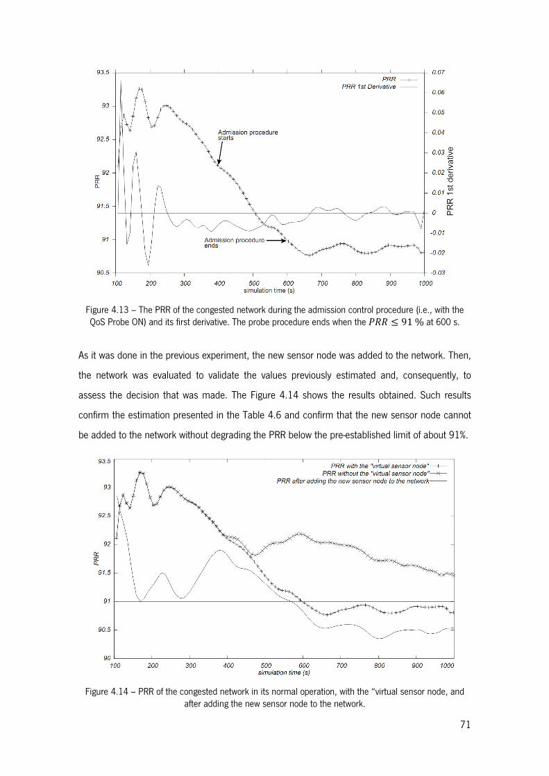
71

Figure 4.13 – The PRR of the congested network during the admission control procedure (i.e., with the QoS Probe ON) and its first derivative. The probe procedure ends when the �� ≤ 91% at 600 s.

As it was done in the previous experiment, the new sensor node was added to the network. Then,

the network was evaluated to validate the values previously estimated and, consequently, to

assess the decision that was made. The Figure 4.14 shows the results obtained. Such results

confirm the estimation presented in the Table 4.6 and confirm that the new sensor node cannot

be added to the network without degrading the PRR below the pre-established limit of about 91%.

Figure 4.14 – PRR of the congested network in its normal operation, with the “virtual sensor node, and after adding the new sensor node to the network.

72

4.5.3. Discussion

During the development stage, several experiments were simulated to assess and, if necessary,

to adjust the proposed QoS-based network management method. The experiments just described

are the result of a continuous process of development and, in that way, they are representative of

the entire development process. Considering the assessment of the QoS monitoring module,

these experiments represent two types of situations, i.e., the detection and classification of both

small QoS degradation events and strong QoS degradation events. On its turn, regarding the

assessment of the QoS-based admission control module, the experiments just described show

how to use the admission control module to verify if a new sensor node can be admitted by both

an uncongested network and a congested network.

In view of the results obtained from the previous simulations, it is possible to argue that the QoS

monitoring module is able to detect and classify suspicious events regarding the degradation of

the QoS provided by the network. Moreover, by using not only the metric value but also its

dynamic, the QoS monitoring module is able to detect and classify QoS degradation events even

before the metric reaches critical values. By using this ability, the QoS monitoring system can be

used to fire advertising messages to the network manager informing about the potential QoS

degradation event. On its turn, the network manager can take measures to mitigate the effects of

such events, preventing the performance of the network from degrading. Regarding the

QoS-based admission control module, it can be used to assess if the network can admit a new

sensor node, i.e., a new patient being monitored. By using a “virtual sensor node” to mimic the

presence of the new real sensor node on its neighbourhood while assessing the network, the

proposed admission control method is able to test the network even from a remote location. In

this way, the proposed QoS-based network management system allows to monitor and manage

the network from a centralised location, which is an important feature regarding patient

monitoring scenarios in hospital facilities or nursing homes.

In view of these results, the QoS-based network management method was considered ready to

be evaluated in a real-wold environment.

73

4.6. Setting the Limit of the Connected Region in Low Power Wireless Links

After the previous evaluation of the proposed QoS-based network management method, it is

necessary to find the conditions under which the proposed method can be used in real-world

environments, as the one presented in the succeeding chapter.

One of the key tenders of this work is that a “virtual sensor node” can simulate the presence of a

real sensor node placed on its neighbourhood. In this way, the scenarios represented in the

Figure 4.15 may be considered equivalent. Taking into consideration the envisioned scenario

(i.e., a set of nursing rooms inside a hospital, as pictured in the Figure 4.1) to use the proposed

method, the Figure 4.15 illustrates the first-hop communications, counting from the sensor

nodes to the sink.

Figure 4.15 – a) A real sensor node simulating the presence of a new sensor node, and b) the new sensor node already within the network.

To mimic the behaviour of the real sensor node, the “virtual sensor node” has to generate data

traffic with the same characteristics as the one generated by the real sensor node. To clarify the

proposed idea, let’s consider the Figure 4.15. The left side scenario shown in the Figure 4.15

(i.e., the Figure 4.15 a)) represents a real sensor node (i.e., the ��2) and a “virtual sensor node” (i.e., the ��5�) created by the ��2, the latter simulating the presence of a new sensor node on its neighbourhood. Each one of these two sensor nodes generate its own data flow, the

��2 generates the data flow /2 and the ��5� generates the data flow /5�. In turn, the scenario represented in the right side of the Figure 4.15 (i.e., the Figure 4.15 b)) portraits the initial

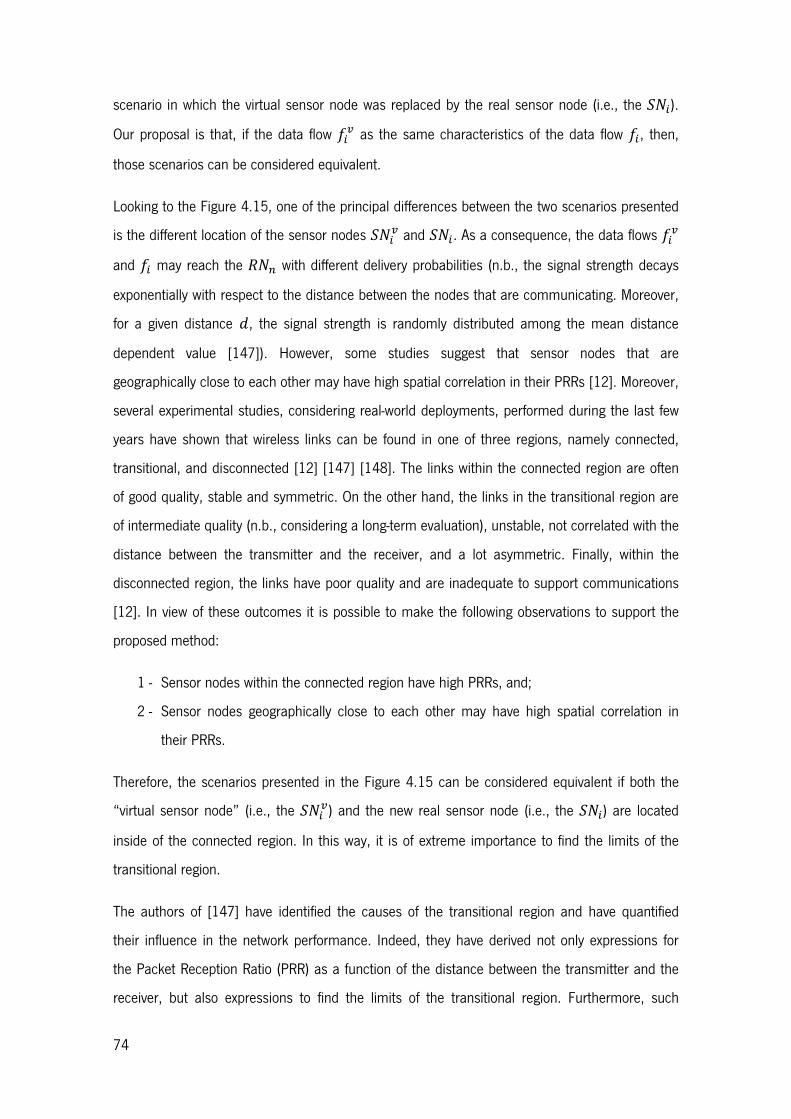
74

scenario in which the virtual sensor node was replaced by the real sensor node (i.e., the ��5). Our proposal is that, if the data flow /5� as the same characteristics of the data flow /5, then, those scenarios can be considered equivalent.

Looking to the Figure 4.15, one of the principal differences between the two scenarios presented

is the different location of the sensor nodes ��5� and ��5. As a consequence, the data flows /5� and /5 may reach the ��z with different delivery probabilities (n.b., the signal strength decays exponentially with respect to the distance between the nodes that are communicating. Moreover,

for a given distance �, the signal strength is randomly distributed among the mean distance dependent value [147]). However, some studies suggest that sensor nodes that are

geographically close to each other may have high spatial correlation in their PRRs [12]. Moreover,

several experimental studies, considering real-world deployments, performed during the last few

years have shown that wireless links can be found in one of three regions, namely connected,

transitional, and disconnected [12] [147] [148]. The links within the connected region are often

of good quality, stable and symmetric. On the other hand, the links in the transitional region are

of intermediate quality (n.b., considering a long-term evaluation), unstable, not correlated with the

distance between the transmitter and the receiver, and a lot asymmetric. Finally, within the

disconnected region, the links have poor quality and are inadequate to support communications

[12]. In view of these outcomes it is possible to make the following observations to support the

proposed method:

1 - Sensor nodes within the connected region have high PRRs, and;

2 - Sensor nodes geographically close to each other may have high spatial correlation in

their PRRs.

Therefore, the scenarios presented in the Figure 4.15 can be considered equivalent if both the

“virtual sensor node” (i.e., the ��5�) and the new real sensor node (i.e., the ��5) are located inside of the connected region. In this way, it is of extreme importance to find the limits of the

transitional region.

The authors of [147] have identified the causes of the transitional region and have quantified

their influence in the network performance. Indeed, they have derived not only expressions for

the Packet Reception Ratio (PRR) as a function of the distance between the transmitter and the

receiver, but also expressions to find the limits of the transitional region. Furthermore, such

75

expressions show how the radio parameters (i.e., the modulation, the encoding, the output power

at the transmitter, the noise floor, and the noise at the receiver), and the environmental

parameters (i.e., the path loss exponent, the log-normal shadow variance, and the noise floor)

influence the length of the transitional region. Bearing those parameters in mind, the transmitter

output power is of utmost importance. It can be easily used to tune the limits of the transitional

region to the needs of each specific application, taking into consideration the particular

characteristics of each environment and the network deployment area. More insights about how

the transmitter output power impact the beginning of the transitional region can be found in [12]

[147] [148].

In view of the scenarios presented in the Figure 4.1 and Figure 4.15, the connected region must

have about 5 m in length around the receiver node (i.e., considering the dimensions of typical

nursing rooms). In other words, the beginning of the transitional region must be at 5 m from the

receiver. Moreover, considering the severe QoS requirements imposed to BWSNs a lower limit of

90 % was imposed to the PRR inside the connected region (n.b., this value can be adjusted

according to the needs of each particular application). Thus, it is necessary to find the minimum

transmitter output power necessary to fulfil those requirements.

In the following, the model presented in [147] will be used to find the minimum output power at

the transmitter necessary to achieve the desired length for the connected region, considering the

PRR limit imposed by the application. Then, in order to fundament the proposed method, it will

be analysed at two levels. First, at the node level, the effects of positioning the sensor nodes at

different locations were investigated in view of single-hop communications. In particular, at the

first hop counting from the sensor node to the sink. Then, the effects of having different delivery

probabilities at single-hop communications are studied at the network level, i.e., considering

multi-hop communications. Our analyse does not consider sensor nodes mobility nor dynamic

objects inside the deployment environment, and the channel conditions for each wireless link are

considered to be constant along the time, or at least during significant time intervals.

4.6.1. Finding the Output Power Necessary to Achieve the Required Connected

Region

In the following we assume NRZ encoding and consider noncoherent FSK modulation scheme

used in TelosB motes [149]. This analysis uses the log-normal shadowing path loss model [150]

76

and the outcomes presented in [147] to find the minimum transmitting power, PK, necessary to achieve a connected region with a radius of 5m. The parameters used to model the indoor environment are: path loss exponent η = 3; standard deviation σ = 4; power decay at reference distance d7, PL"d7$ = 55dB; noise floor P� = −105dBm; and the size of the frames used to communicate is f = 70bytes. Let us bound the connected region to PRRs greater than 0.9 and the transitional region to PRRs

between 0.9 and 0.1. From the theoretical model deduced in [147], we obtain the following SNR

values for PRRs of 0.1 and 0.9, γ�R� and γ�R�, respectively, γ�R� = 10log47 �−1.28ln �2 �1 − 0.14�� ¡ ≈ 7.9dB, Eq. 4.14

γ�R� = 10log47 �−1.28ln �2 �1 − 0.94�� ¡ ≈ 10.0dB, Eq. 4.15

and we have

PK = P� + γ� + PL"d7$ + 2σ + 10η log47 dO ≈ −11 dBm Eq. 4.16

for the minimum transmitting power necessary to achieve the necessary length for the connected

region. In the following sections we analyse if a “virtual sensor node” can simulate the presence

of a real sensor node placed in the connected region of 5 m in length.

4.6.2. Analysing the Virtual Sensor Node’s PRR Considering Single-hop

Communications

Consider the scenario presented in the Figure 4.15. To obtain the maximum difference between

the PRR achieved by both the virtual data flow f�¦ and the real data flow f�, considering only first-hop (i.e., the link between the SN�¦, or the SN�, and the RN�), we use the equation of PRR at a transmitter-receiver distance d obtained in [147]:

p"d$ = �1 − 12 exp�−γ"d$1.28 ¡��, Eq. 4.17

where γ"d$R� = PKR� − PL"d$R� − P�R�, PL"d$R� = PKR� − PMR�, and PMR� is the received signal strength at a given distance d from the transmitter. From [150] we have

PL"d$ = PL"d7$ + 10ηlog47"d d7⁄ $ + X7,«, whereX7,« is a zero-mean Gaussian random variable (in dB) with the standard deviationσ (shadowing effects). First, we obtain a relationship

77

between pHd�,�Iand pHd�,� + Δd�,�I for an increment Δd�,� at the distance d�,� between SN� and RN�. Using the Taylor’s theorem for the case n = 1 at the point d�,�, we have:

p"d$ = pHd�,�I + p< Hd�,�IΔd�,� + R�,�, Eq. 4.18

where R�,� is the remainder term. By properties of (1) we can state that the remainder term R�,� is residual in the interval ®0, 5® and (2) with R�,� = 0 is a good linear approximation to (1) on ®0, 5®. Then, we have pHd�,� + Δd�,�I − pHd�,�I = p< Hd�,�IΔd�,�, where

p< Hd�,�I = − 8fαβη2.56d�,� k1 −α2l

��34, Eq. 4.19

α = exp"−β 1.28⁄ $ and β = 10H²³3²�"R´$347µQP¶·´HR¸,¹I3²¹I 47⁄ = 10º.»3ºQP¶·´HR¸,¹I. Since (3) is a decreasing non-positive function we obtain that maxR¸,¹∈®7,¼®?p< Hd�,�I? = |p< "5$|. Thus, we obtain ?p< Hd�,�I? ≤ 2.3 × 1034�. Therefore, since Δd�,� ∈ ®0, 5®, we have ?pHd�,� +Δd�,�I − pHd�,�I? ≤ 1.2 × 1034¿ ≈ 0 in the connected region of 5 m in length. Thus, the difference between the PRR achieved by both the virtual data flow f�¦ and the real data flow f�, considering only first-hop, is approximately equal to zero.

4.6.3. Analysing the Virtual Sensor Node’s PRR Considering Multi-hop

Communications

Rather than single-hop communications, typical BWSNs have multiple hops between the source

sensor nodes and the sink. In fact, they may have not only several hops between those nodes but

also several paths to route the data gathered by the sensor nodes to the sink. In that way, two

sensor nodes can send their data to the sink using distinct data paths, each one having a

particular PRR associated. In our proposal we consider that the data flow /5�, generated by the “virtual sensor node” ��5� of the Figure 4.15 a), follows the best path to reach the sink (n.b., the rule to find the best path depend on the routing protocol in use). Moreover, the sensor node ��5 will use the same path to send its data to the sink. In other words, we are assuming that both the

“virtual sensor node”, ��5�, and the real sensor node, ��5, use the same data path to send their data to the sink. In this way, the PRR associated with the path between the ��z and the sink is the same for both data flows. Additionally, as it was shown in the last subsection, the PRRs

achieved by both the virtual data flow /5� and the real data flow /5 at the first hop are similar.

78

Consequently, it is possible to argue that the PRRs of both data flows, for the entire path (i.e.,

from the sensor node until the sink) are equivalent.

In summary, our proposal is that a “virtual sensor node” can produce the same effect in the

performance of a WSN, when compared with a real sensor node, if both sensor nodes produce

data with the same characteristics, both data flows follow the same path to the sink, and they are

within the connected region experiencing the same radio conditions.

4.6.4. Experimental Validation

On the basis of the previous requirements, the experiment described in the Figure 4.16 was

performed to assess the model used in the sections 4.6.1 and 4.6.2.

Figure 4.16 – Experiment performed to find the minimum transmitter output power needed to have at least a PRR of about 90 % inside a region of 5 m around the receiver (i.e., inside the connected region).

The experiment is as follows: inside a typical deployment area (n.b., the experiment was

performed using an environment designed to recreate the conditions inside a nursing room), with

fixed obstacles and metal furniture, a sink node and a sensor node were used to measure the

PRR at different distances between the two nodes and for several angles all around the receiver

as pictured in the Figure 4.16, in order to find the minimum transmitter output power to achieve

a PRR of, at least, 90 % inside the connected region and set the beginning of the transitional

region to 5 m from the transmitter. The PRR for each pair (distance, angle) was calculated after

the sensor node had sent five hundreds messages to the receiver.

The Figure 4.17 shows the results obtained when assessing the PRR for different distances

between the sender sensor node and the receiver. In that case the transmitter output power was

set to −25��. The results obtained show that for a distance of 2 m between the source

79

sensor node and the receiver (i.e., the Figure 4.17 a)), the PRR fits within the pre-established

limit of 90%. However, when changing the distance between the sender and the receiver to 3 m

(i.e., the Figure 4.17 b)) the PRR for an angle of 72º between the sender and the sink is of about

85 % which is beyond the pre-established limit of 90 %. So, it is possible to conclude that the

transmitter output power must be greater than −25�� in order to fulfil the required PRR.

Figure 4.17 – PRR for an output power of −25�� at the transmitter, for distances of 2 and 3 meters

between the transmitter and the receiver.

Figure 4.18 – PRR for an output power of −15�� at the transmitter, for distances of 2 and 3 meters

between the transmitter and the receiver.

Proceeding with the experiment, the output power of the sender sensor node was changed to

−15�� and the experiment repeated. The Figure 4.18 shows the results obtained. Analysing

80

the Figure 4.18 b) it is possible to verify that the PRR for an angle of 108º, between the sender

and the sink, is of about 87%, which is lower than the pre-established limit of 90%. Consequently,

an output power of −15�� at the sender is insufficient to achieve a connected region of

about 5 m with the desired characteristics.

Figure 4.19 – PRR for an output power of −10�� at the transmitter, for distances of 2, 3, 4 and 5

meters between the transmitter and the receiver.

The Figure 4.19 shows the results obtained when repeating the previous experiment considering

an output power of −10dBm at the sender. From the results, it is possible to see that the PRR

for all the tested distances (i.e., distances of 2, 3, 4 and 5 meters between the sender and the

sink), all around the sink, is always greater than the pre-established threshold of 90%. Therefore,

it is possible to argue that the minimum output power at the transmitter necessary to achieve a

connected region of 5 m in length is −10dBm, as predict in the section 4.6.1 by the analytic

81

model. It is important to notice that these results depend on each specific environment and

network deployment area. Consequently, these results must be tuned for each network

deployment.

4.7. Summary

This chapter presented the proposed QoS-based network management method, its application

scenario, and some experiments performed during the development stage to assess it.

The proposed QoS-based network management method is composed by two modules: the

QoS-based admission control module and the QoS monitoring module. The QoS-based admission

control module uses the concept of “virtual sensor node” to estimate the impact of adding new

sensor nodes to the BWSN and thereby assess the network about its ability to accommodate a

new sensor node while maintaining the QoS required by all the applications using the BWSN. On

its turn, the QoS monitoring system uses a mathematical framework to detect and classify

potential degradation events.

Since its presentation, the QoS-based network management method was carefully tested. In view

of the results obtained not only from several simulations performed during the development

stage, but also from analytic and experimental analysis regarding the quality of low power

wireless links, it is possible to argue that the proposed method can be used both to estimate the

impact of adding new sensor nodes to the network and to detect and classify potential QoS

degradation events.

Finally, have been defined the conditions under which the proposed method can be used in

real-world environments.

83

Chapter 5

Method Assessment in a Real Hospital

Environment

Real-World Assessment

5.1 Preliminary Findings and Initial Deployment

5.1.1 Preliminary Findings

5.1.2 Initial Deployment

5.2 QoS-Based Admission Control Module Assessment

5.2.1 Network Deployment Area Covering One Nursing Room

5.2.2 Network Deployment Area Covering Two Nursing Rooms

5.2.3 Network Deployment Area Covering Three Nursing Rooms

5.2.4 Discussion

5.3 Summary

85

5. Method Assessment in a Real Hospital Environment

The proposed QoS-based network management method was carefully tested during the

development stage using different approaches, namely: simulated environments, probabilistic

models, and empiric experiments. Although these tests may be considered sufficient to validate

the QoS monitoring module (n.b., the QoS monitoring module operation depends only on the

metric behaviour, rather than on the network deployment environment), they are insufficient to

validate the QoS-based admission control module. Therefore, the QoS-based admission control

module was evaluated in a real hospital environment.

The remainder of this chapter describes not only the real-world experiments performed to

evaluate the QoS-based admission control module, but also their preparation. The experiments

were made in a small-sized hospital situated in Esposende, a small city near Braga, Portugal; the

hospital is known as “Hospital Valentim Ribeiro”.

5.1. Preliminary Findings and Initial Deployment

The deployment of BWSNs in real-world environments is a challenging task even to engineers

with high levels of expertise in BWSNs systems. Moreover, when harsh environments are at

stake, such as hospital facilities or nursing homes, the difficulties to get BWSNs working properly

worsens. Hence, each real-world BWSN deployment must be carefully designed not merely

according to the demands of each target application, but also considering the particular

characteristics of each deployment area.

5.1.1. Preliminary Findings

Based on the knowledge obtained from this particular deployment, it is possible to argue that

each real-world deployment is unique. More, it is strictly necessary to study and understand the

intrinsic characteristics of each deployment site, namely those that can compromise the quality

of the wireless channel, such as: attenuation of the radio signal caused by metallic furniture,

interferences caused by other medical equipment’s, and other negative effects caused by

peoples’ routines (e.g., staff shifts or visiting times). Such study is vital to design a suitable

network deployment strategy in order to achieve the required performance.

86

Regarding the deployment scenario used to evaluate the proposed QoS-based admission control

method, the following procedure was made in order to understand the intrinsic characteristics of

the network deployment site. First, information was collected about the use made of the network

deployment area. Second, an inspection was made to identify other radio communication

infrastructures (e.g., an IEEE802.11 network) existing on the network deployment area. Third, an

examination was made to find hospital furniture and/or medical equipment able to cause

attenuation/interferences in the radio signals (e.g., fading due to multipath or due to shadowing

from obstacles). Finally, information was requested about the hospital staff shifts and about the

visiting schedule.

It is important to emphasise that the research team had no control on the environment

conditions, or on the use of any hospital/medical equipment, during the field tests. All the tests

were made under the supervision of the hospital staff.

The area used to perform the field tests (i.e., the shaded area presented in the Figure 5.1) has a

nursing desk and three nursing rooms in which low-acuity patients stay for a period that, typically,

do not exceed eight days. Those nursing rooms are not private, if necessary two or three patients

can share the same room.

Figure 5.1 – Floor plan of the Hospital Valentim Ribeiro. The shaded areas show the nursing rooms and the nursing desk used to deploy the BWSN.

Rooms

Nursing Desk

87

From our survey, it was found that the deployment area does not have any other wireless

communication technology. Instead, the information system uses a wired communication

infrastructure. Therefore, it was not necessary to perform any tests to study the radio activity on

the deployment area. When other wireless communication technologies are detected, it is

necessary to study the coexistence of both technologies, as explained by JeongGil Ko in [151].

Concerning the signal propagation and electromagnetic interferences (or any other effect able to

deteriorate the radio signal), neither the hospital furniture nor the medical equipment found in

the deployment area is susceptible of causing significant damages to the radio channel. On its

turn, the staff daily routines can be classified as regular concerning the normal activities of a

non-acute hospital area. So, on this particular deployment area, the radio signal propagation is

affected only by the building structure (e.g., walls, corridors or steel doors) and by the human

bodies present on the site. During the field tests the average amount of people inside of the

network deployment area, simultaneously, did not exceeded a dozen. So, the network

deployment area can be considered as having low density of people.

5.1.2. Initial Deployment

After the preliminary study just described, it was necessary to design the network deployment

strategy. First, the network physical topology was defined. Following the strategy proposed by the

MEDiSN project [2] [49], the solution adopted makes use of a backbone of Relay Nodes (RNs)

and several Sensor Nodes (SNs), defining a tree topology as represented in the in Figure 5.2. As

explained by the authors of the MEDiSN project, the backbone is used both to form a

bidirectional link to the Sink and to ensure the required network coverage. Moreover, the use of a

backbone has several benefits. It allows expanding the network, both to improve its performance

(e.g., by carefully placing more RNs in the same area) and to increase the network coverage (i.e.,

improving the network scalability).

Since the nursing staff will use information retrieved by the proposed QoS-based admission

control method to make a decision about the best location to place the patients, the natural

location to place the sink is the nursing desk, so it can be connected to the computer running the

frontend interface of the network management system. The backbone contains two RNs strategic

placed to ensure good connectivity inside the nursing rooms three and four. On its turn, the SNs

inside the nursing room five can connect directly to the sink.

88

Figure 5.2 – The network topology makes use of a backbone of relay nodes to ensure the necessary coverage and to route the data packets to the sink.

Figure 5.3 shows the deployment of both the sink and the backbone (n.b., the links between the

RNs within the backbone and between the RNs and the sink are merely for example purposes. In

reality, the backbone is self-organized).

Figure 5.3 – Initial deployment, showing the relay nodes forming a backbone to the sink.

Several tests were made in order to determine the best spots to set up the RNs, while ensuring

both the necessary network coverage and the required network performance. To assess the

network’s performance the end-to-end PRR was used as figure-of-merit. Based on the tests

performed the RNs were deployed as shown in the Figure 5.3. After deploying the RNs backbone,

the BWSN became fully functional and ready to admit the patients, i.e. the sensor nodes.

89

5.2. QoS-Based Admission Control Module Assessment

In the following all the experiments performed to evaluate the QoS-based admission control

module are explained in detail, in particular the use of a “virtual sensor node” to mimic the

presence of a new real sensor node within the network.

The evaluation procedure was made in three distinct scenarios, according to the number of

nursing rooms used and patients being monitored. By using different nursing rooms, it was

possible to assess the proposed method taking into account the impact of the hospital structure

(e.g., granite walls, corridors and doors) on the propagation of the radio signals and,

consequently, on the network performance. On its turn, the use of several patients makes the

experiments closer to reality, assessing the suggested method under realistic conditions.

In the first scenario, no more than three patients were monitored while sharing the same nursing

room (i.e., the room 4 from Figure 5.3). This scenario was designed to assess the proposed

method without interferences from patients being monitored in the neighbourhood and, at the

same time, experiencing the minimum impact from the deployment environment. By using this

scenario, the proposed method will be used to assess the impact of adding a new patient to the

network.

Then, in the second scenario, a maximum of five patients were monitored while distributed by

two non-adjacent nursing rooms (i.e., the rooms 3 and 4, separated by two bathrooms, as

pictured in the Figure 5.3). This scenario was designed to assess the suggested QoS-based

admission control method under interferences from patients being monitored in the

neighbourhood of the “virtual sensor node”. Moreover, this scenario is also useful to study the

impact of using the proposed method, on the patients being monitored in the neighbourhood of

the “virtual sensor node”.

Finally, in the third scenario, a maximum of five patients were monitored while distributed by

three nursing rooms (i.e., the rooms 3, 4, and 5 from Figure 5.3). This scenario was designed to

evaluate the impact of the building structure when using the proposed method. All these

scenarios were designed with the purpose to verify the following hypothesis:

Hypothesis: Adding a “virtual sensor node” to a BWSN produces an equivalent

impact in the network’s performance, when comparing with the addition H. 5.1

90

of a new real sensor node.

If this hypothesis was confirmed, the proposed QoS-based admission control module can be used

to answer the following questions:

• Which is the impact of adding a new patient to a BWSN, in the QoS being provided to the

patients already within the network?

• Which is the best location to add a new patient to a BWSN, while minimising its impact in

the QoS being provided by the network?

In such context, all the experiments were performed under the following assumptions:

• The term patient is only a nomenclature used to improve the understanding of the

experiments. In reality, they are represented by the sensor nodes;

• The physiologic data are generated by the sensor nodes;

• The mobility of the sensor nodes is very limited and unable to cause changes in the

network topology (i.e., in both the physical and logical topologies).

Table 5.1 – Application and network level configurations common to all the experiments.

Application: Operating System Contiki OS Task type Time driven Data length 70 bytes (per packet) Data reporting interval 500 ms QoS-probe reporting interval 500 ms Network: Number of sinks 1 Number of relay nodes 2 Number of sensor nodes 3, 4, 5 (depending on the scenario being assessed) Transmission power 0 dBm (in both, the sink and the RNs), -7 dBm or -10 dBm (in the SNs) Network Layer IPv6 with 6LowPAN Transport Layer UDP Routing protocol RPL – DIO minimum interval 65 s and DIO maximum interval 70 minutes Experiments: Time Between 90 and 120 minutes

Regarding the patient monitoring application used to perform the experiments, its purpose is to

monitor three vital signs (i.e., temperature, heart rate, and respiratory rate) and the oxygen

saturation (SpO2). To do so, each sensor node generates data traffic according to the

91

characteristics of each one of these signals, resulting in an aggregated data rate of about 1 kbps,

considering the reference values of the Table 3.4. For a detailed description of the application

and network configurations see Table 5.1.

Regarding the results obtained from the experiments, they were analysed considering not only all

the stages of the admission control procedure, but also the results obtained when adding the new

real sensor node to the BWSN. Regarding the admission control procedure, it can be divided into

two different time intervals: the time interval from the beginning of the experiment until the

instant when the QoS Probe is turned ON, denoted as: t ∈ Á0, tÂPÃ²MPÄNÅÆÁ; and the time interval in which the QoS Probe is sending data packets to the sink, denoted as: t ∈ÁtÂPÃ²MPÄNÅÆ, tÂPÃ²MPÄNÅÇÇÁ. After the admission control procedure, it is possible to identify two more important time intervals, namely: the time interval between the end of the admission

procedure and the instant when the new real sensor node is admitted to the BWSN, denoted as:

t ∈ ÁtÂPÃ²MPÄNÅÇÇ, tÆNÈÃÆÅÆÁ; and the time interval in which the new real sensor node is sending data packets to the sink, denoted as: t ∈ ®tÆNÈÃÆÅÆ, tÆNÈÃÆÅÇÇ®. As it was done when assessing the proposed QoS-based admission control module using

simulated environments, as described in the chapter 4, the PRR is taken as figure-of-merit to

evaluate the QoS provided by the network. The PRR of each sensor node was defined as:

��5 = �� , Eq. 5.1

where the ��5 is the PRR of the sensor node ��5, �5 is the number of data packets received by the sink from the ��5, and �5 is the number of data packets sent by the ��5.

5.2.1. Network Deployment Area Covering One Nursing Room

This scenario, i.e., monitoring a maximum of three patients sharing the same nursing room, was

designed to verify if the proposed QoS-based admission control module could be used to answer

the following question:

Question: Is it possible to use the concept of “virtual sensor node” to estimate the

QoS impact of adding a new patient to a BWSN, considering that all the

sensor nodes share the same physical space?

Q. 5.1

92

Seeking the answer for this question, the following scenario, comprising two patients being

monitored while sharing the same physical space (i.e., the same nursing room), was designed.

In such case, the proposed QoS-based admission control method can be used to investigate the

impact of adding a third patient to the BWSN, while sharing the same physical space with the

other two patients, in the QoS being provided by the network. Finally, considering the results

retrieved by the QoS-based admission control module, it is possible to decide whether the new

patient can be added to that nursing room or, in the contrary, the new patient must be placed in

a different nursing room.

Several experiments were performed in the context of this scenario. Among all the performed

experiments, the following two were chosen to be analysed. These experiments were chosen to

be analysed due to the different paths used by the QoS probe to send its data to the sink. The

first experiment shows a BWSN in which all the sensor nodes send their data packets to the sink

through the RN4, as pictured in the Figure 5.4. In such case, all the sensor nodes are using the same wireless link to communicate with the sink, consequently, the wireless link can become

saturated and the addition of a new sensor node to the network can result in a substantial

degradation of the QoS being provided by the network. On its turn, in the second experiment, the

data packets reach the sink following two distinct paths, since one sensor node sends its data

packets to the sink through the RN4 and the other sensor node is directly connected to the sink as depicted in the Figure 5.9. In such case, the communications links are less congested and the

addition of a new sensor node to the BWSN has less impact in the QoS being provided by the

network, when comparing with the previous network logical topology. The following discussion

analyses the results obtained when assessing this scenario considering the network logical

topologies just described.

5.2.1.1. Using the same data path to route the data to the sink

Considering this particular scenario, and the network logical topology represented in the Figure

5.4 and Table 5.2, the results obtained by using the proposed admission control method to

assess the BWSN and decide if a new patient can be added to it are presented in the Figure 5.5,

Figure 5.6, Figure 5.7, and Figure 5.8. To facilitate its analysis and discussion, such results are

summarised in the Table 5.3. It is important to highlight that, regarding this particular

experiment, the network was under the influence of external interferences during the admission

93

control procedure, as pictured in the Figure 5.5, Figure 5.6, and Figure 5.7. Such interferences

were related with the presence of an abnormal number of persons in the corridors due to the

visiting schedule, the lunchtime and the cleaning staff. The results presented in the Table 5.3

were obtained after removing the effect of such interferences.

Figure 5.4 – The BWSN used to monitor three patients sharing the same nursing room. In such network logical topology, all the patients (i.e., the SN4, the SN� and theSNº) sent their data packets to the sink

through the backbone. Table 5.2 shows the sink’s routing table regarding this topology.

Table 5.2 – The sink’s routing table for the network topology pictured in the Figure 5.4.

Destination Next hop

Node ID: Node IP: Node ID: Node IP: ��4 AAAA::0212:7400:13CB:2777 ��4 FE80::0212:7400:13CB:2777 ��4 AAAA::0212:7400:13CA:FDCA ��4 FE80::0212:7400:13CB:2777 �� AAAA::0212:7400:13CA:E837 ��4 FE80::0212:7400:13CB:2777 ��º AAAA::0212:7400:13CB:2128 ��4 FE80::0212:7400:13CB:2777

Table 5.3 – Results obtained when assessing the BWSN considering the network topology presented in the Figure 5.4.

Network Running Time (t)

Packet Reception Ratio HÉ�� ± ËI%

��4 (Figure 5.5)

�� (Figure 5.6)

QoS Probe (Figure 5.7)

New SN (��º) (Figure 5.8)

t ∈ Á0, tÂPÃ²MPÄNÅÆÁ 99.1 ± 0.9 98.9 ± 1.1 n.a. n.a.

t ∈ ÁtÂPÃ²MPÄNÅÆ, tÂPÃ²MPÄNÅÇÇÁ ÌÍ. Î ± Î. Î ÍÏ. Ð ± Ñ. Ï Í�. Ï ± �. Ò n.a.

t ∈ ÁtÂPÃ²MPÄNÅÇÇ, tÆNÈÃÆÅÆÁ 98.9 ± 1.1 98.2 ± 1.8 n.a. n.a.

t ∈ ®tÆNÈÃÆÅÆ, tÆNÈÃÆÅÇÇ® ÍÑ. Ó ± �. Ï ÍÓ. Ð ± Î. Ó n.a. ÍÎ. Ô ± Î. �

94

Initially the network was being used to carry the data generated by two patients (i.e., the SN4 and the SN�). In such case, the network can be considered highly efficient and providing high standards of QoS. Such fact can be confirmed by analysing the PRR of the data flows generated

by both sensor nodes, during the time periods: t ∈ Á0, tÂPÃ²MPÄNÅÆÁ and

t ∈ ÁtÂPÃ²MPÄNÅÇÇ, tÆNÈÃÆÅÆÁ. To be precise, during these two time intervals, the �� of the data flow generated by the SN4 is of about 99.1% and 98.9%, respectively. On its turn,

the �� related to the data flow generated by the SN�, during the same time intervals, is of about 98.9% and 98.2%, respectively. Then, when using the QoS Probe to assess the

possibility of adding a new patient to the network, sharing the same nursing room, which

comprises the interval t ∈ ÁtÂPÃ²MPÄNÅÆ, tÂPÃ²MPÄNÅÇÇÁ, the PRR of the data flows generated by both the SN4 and the SN� drops considerably. Indeed, the �� of the data flow generated by the SN4 drops about 9.7pp from 99.1% to 89.4% and the �� of the data flow generated by the SN� drops from about 98.9% to90.6%, corresponding to a degradation of

about 8.3pp. On its turn, the �� achieved by the QoS Probe is around92%, which is

comparable with the values achieved by the other sensor nodes. Such degradation in the PRR of

both data flows can be justified by the additional traffic generated by the QoS Probe. In fact, such

additional traffic makes the competition for the transmission medium more difficult, increasing

the probability of collisions as well as the interferences experienced by each sensor node, not

only due to the presence of the QoS Probe within the network but also due to the additional

retransmissions performed by the RN4.

Finally, after the admission of the SNº (i.e., the new patient), that corresponds to the time interval t ∈ ®tÆNÈÃÆÅÆ, tÆNÈÃÆÅÇÇ®, the �� of the data flows generated both by the SN4 and by the SN� falls about 3.6pp, from 98.9% to 95.3%, and 4.6pp, from 98.2% to

93.6%, respectively. On its turn, the �� of the data flow generated by the SNº is of about 94.1%, which is comparable with the PRR achieved by the other sensor nodes. In that case, the

degradation on the PRR can also be explained using the arguments presented earlier. However,

since the data generation processes are not time synchronised, the impact of adding the sensor

nodes (i.e., the QoS Probe and the SNº) in different moments affects the performance of the network in diverse ways.

95

Figure 5.5 –PRR of the data flow generated by the SN4 during the admission control procedure regarding

the network logical topology presented in the Figure 5.4.

Figure 5.6 – PRR of the data flow generated by the SN� during the admission control procedure regarding

the network logical topology presented in the Figure 5.4.

The PRR of the data flows generated by SN4 and SN� are shown in the Figure 5.5 and Figure 5.6, respectively. Looking to those figures, it is possible to identify all the phases of the

experiment, namely the network on its typical operation, the network being assessed using the

proposed QoS-based admission control method, and the network operation after the addition of

the new patient. Regarding the PRR during the network typical operation, it can be found in two

different time intervals, t ∈ ®0, 3000®s and t ∈ ®9300, 11200®s , where the PRR is similar in both sensor nodes.

Figure 5.7 shows the PRR of the data flow generated by the QoS Probe (i.e., the “virtual sensor

node”). The strong PRR degradation that can be observed in the time interval 5000 s – 7000 s

results from external interferences, as already explained. Apart from that region, the �� is of about 92%.

96

Figure 5.7 – PRR of the data flow generated by the QoS Probe during the admission control procedure

regarding the network logical topology presented in the Figure 5.4.

Figure 5.8 – PRR of the data flow generated by the new sensor node (i.e., the SNº) during the admission

control procedure regarding the network logical topology presented in the Figure 5.4.

Finally, the PRR of the data flow produced by the new patient (i.e., theSNº) is shown in Figure 5.8 where it can be observed that theSNº had a setup time extremely long, of about 12 minutes. Such abnormal and unexpected situation was not repeated during the field tests. After

this setup time, the �� becomes stable at a value of about94.1%.

The previous per sensor node analysis investigated the effect of each phase of the experiment in

the PRR achieved by each data flow carried by the network. Nevertheless, such individual

analysis is not sufficient to forecast the QoS provided by the network after adding the new sensor

node, based on the QoS provided during the assessment phase. To that end, it is necessary to

compare the PRR achieved during those time intervals. So, to study the similarity between the

PRRs of each data flow during the assessment period and after adding the new sensor node to

the network, the percentage difference was used:

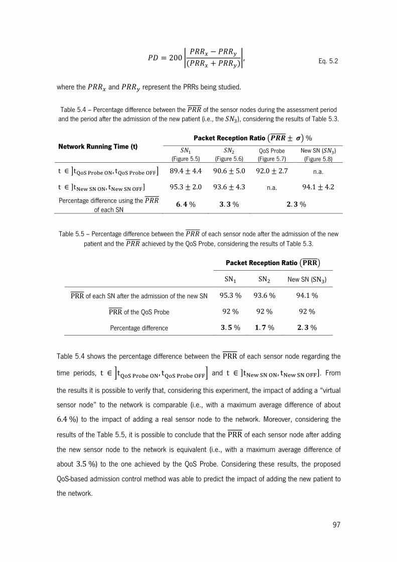
97

�U = 200 Ö ��y − ��×"��y + ��×$Ö, Eq. 5.2

where the ��y and ��× represent the PRRs being studied. Table 5.4 – Percentage difference between the �� of the sensor nodes during the assessment period and the period after the admission of the new patient (i.e., the��º), considering the results of Table 5.3.



��4 (Figure 5.5)

�� (Figure 5.6)



t ∈ ØtÂPÃ²MPÄNÅÆ, tÂPÃ²MPÄNÅÇÇØ 89.4±4.4 90.6±5.0 92.0±2.7 n.a.t ∈ ®tÆNÈÃÆÅÆ, tÆNÈÃÆÅÇÇ® 95.3±2.0 93.6±4.3 n.a. 94.1±4.2Percentage difference using the ��

of each SN Ð. Î% Ó. Ó% �. Ó%

Table 5.5 – Percentage difference between the �� of each sensor node after the admission of the new patient and the �� achieved by the QoS Probe, considering the results of Table 5.3.

Packet Reception Ratio HÙÚÚI SN4 SN� New SN (SNº)

PRR of each SN after the admission of the new SN 95.3% 93.6% 94.1%

PRR of the QoS Probe 92% 92% 92%

Percentage difference Ó. Ñ% Ô. Ò% �. Ó%

Table 5.4 shows the percentage difference between the PRR of each sensor node regarding the time periods, t ∈ ÁtÂPÃ²MPÄNÅÆ, tÂPÃ²MPÄNÅÇÇÁ and t ∈ ®tÆNÈÃÆÅÆ, tÆNÈÃÆÅÇÇ®. From the results it is possible to verify that, considering this experiment, the impact of adding a “virtual

sensor node” to the network is comparable (i.e., with a maximum average difference of about

6.4%) to the impact of adding a real sensor node to the network. Moreover, considering the

results of the Table 5.5, it is possible to conclude that the PRR of each sensor node after adding the new sensor node to the network is equivalent (i.e., with a maximum average difference of

about 3.5%) to the one achieved by the QoS Probe. Considering these results, the proposed

QoS-based admission control method was able to predict the impact of adding the new patient to

the network.

98

5.2.1.2. Using different data paths to route the data to the sink

This scenario was also evaluated using the network topology presented in the Figure 5.9 and

Table 5.6. In this case the data produced by the sensor nodes follow two distinct paths to reach

the sink. This change in the network logical topology reduces the impact of adding a new patient

to the network in the QoS being provided, as it can be seen in the results presented in the Table

5.7. The existence of two alternative paths to route the data to the sink decreases not only the

occupation of the wireless link containing the RN4 (i.e., the data traffic through the RN4) but also the level of interferences, since the data sent by the SN4, which is directly connected to the sink, do not need to be forwarded as in the logical topology presented in the Figure 5.4.

Figure 5.9 – The BWSN used to monitor three patients sharing the same nursing room. In such network logical topology, two patients (i.e., the SN� and the SNº) sent their data to the sink through the backbone and the other one (i.e., the SN4) is directly connected to the sink. Table 5.6 shows the sink’s routing table

regarding this topology.



Node ID: Node IP: Node ID: Node IP: ��4 AAAA::0212:7400:13CC:392F ��4 FE80::0212:7400:13CC:392F ��4 AAAA::0212:7400:13CA:FDCA ��4 FE80::0212:7400:13CA:FDCA �� AAAA::0212:7400:13CA:E837 ��4 FE80::0212:7400:13CC:392F ��º AAAA::0212:7400:13CB:2128 ��4 FE80::0212:7400:13CC:392F

99

The results obtained when using the suggested QoS-based admission control method to assess

the BWSN pictured in the Figure 5.9, in order to make a decision about the admission of a new

patient to the network, are presented in the Figure 5.10, Figure 5.11, Figure 5.12 and Figure

5.13, and are summarised in the Table 5.7.

Table 5.7 – Results obtained when assessing the BWSN considering the network topology presented in the Figure 5.9.



��4 (Figure 5.10)

�� (Figure 5.11)



t ∈ Á0, tÂPÃ²MPÄNÅÆÁ 99.8 ± 0.2 99.9 ± 0.1 n.a. n.a.

t ∈ ÁtÂPÃ²MPÄNÅÆ, tÂPÃ²MPÄNÅÇÇÁ ÍÍ. Ñ ± Ï. Î ÍÌ. Ï ± Ï. Ò ÍÍ. Ò ± Ï. Ó n.a.

t ∈ ÁtÂPÃ²MPÄNÅÇÇ, tÆNÈÃÆÅÆÁ 99.6 ± 0.4 99.6 ± 0.3 n.a. n.a.

t ∈ ®tÆNÈÃÆÅÆ, tÆNÈÃÆÅÇÇ® ÍÌ. Í ± Ï. Ò ÍÌ. Ð ± Ï. Í n.a. ÍÌ. Ì ± Ô. �

As in the previous experiment, at the beginning the BWSN was being used to carry the data

produced by two patients (i.e., the SN4 and the SN�). In such time period, the network was providing high levels of QoS, as it can be confirmed by the values of the PRR achieved by both

sensor nodes, during the time periods: t ∈ Á0, tÂPÃ²MPÄNÅÆÁ ∪ ÁtÂPÃ²MPÄNÅÇÇ, tÆNÈÃÆÅÆÁ. Indeed, to be accurate, the �� of the data flow generated by the SN4 was of about 99.8%

and 99.6%, respectively. On its turn, the �� related to the data flow generated by the SN� was of about 99.9% and 99.6%, respectively. Then, contrasting with the previous experiment,

the PRR of the data flows within the network does not significantly change during the assessment

period (i.e., during the period of t ∈ ØtÂPÃ²MPÄNÅÆ, tÂPÃ²MPÄNÅÇÇØ) and after the addition of the new patient (i.e., during the period of t ∈ ®tÆNÈÃÆÅÆ, tÆNÈÃÆÅÇÇ®). In fact they all remain, in average, above98%.

The PRR of the data flows produced by the SN4 and by the SN� is pictured in the Figure 5.10 and Figure 5.11, respectively. Analysing those figures, it is possible to conclude that, apart from

the time period corresponding to the network assessment, using the proposed admission control

method (i.e., the time interval includingt ∈ ®2000, 3700®s), the PRRs of both sensor nodes are very similar. To be precise, the �� of both sensor nodes are 98.9% and 98.6% to the

SN4 and SN�, respectively. On its turn, during the time interval comprising the assessment

100

period, the �� of the data flow generated by the SN� is of about98%. Which is 1.5pp below the value achieved by theSN4 (i.e.,99.5%).

Figure 5.10 – PRR of the data flow generated by the SN4 during the admission control procedure regarding the network logical topology presented in the Figure 5.5.

Figure 5.11 – PRR of the data flow generated by the SN� during the admission control procedure regarding the network logical topology presented in the Figure 5.5.

Figure 5.12 shows the PRR of the data flow generated by the QoS Probe. During the QoS Probe

operation, the PRR associated with its data flow is of about 99.7%. On its turn, the Figure 5.13

shows the PRR of the data flow produced by the SNº (i.e., the new patient). In this case, the PRR is of about 98.8%.

101

Figure 5.12 – PRR of the data flow generated by the QoS Probe during the admission control procedure regarding the network logical topology presented in the Figure 5.5.

Figure 5.13 – PRR of the data flow generated by the new SN (SNº) during the admission control procedure regarding the network logical topology presented in the Figure 5.5.

Following the analysis of the former experiment, it is necessary to relate the PRR achieved by the

sensor nodes during both the assessment period using the proposed method and the period after

the admission of the new patient within the network. As before, this analysis was made using the

percentage difference (i.e., Eq. 5.2). Table 5.8 presents the percentage difference concerning the

PRR of each sensor node within the network for the time periods being studied. Analysing the

results, it is clear that the difference between the PRR of the data flows produced by the sensor

nodes within the network during the periods being studied is minimal, as expected, once the data

paths within the network are uncongested. Furthermore, looking to the results presented in the

Table 5.9, it is possible to verify that the �� of each patient after the admission of the new patient is comparable to the one achieved by the QoS Probe during the network assessment

period. As earlier, the proposed QoS-based admission control method was able to predict the

impact of adding the new patient to the network.

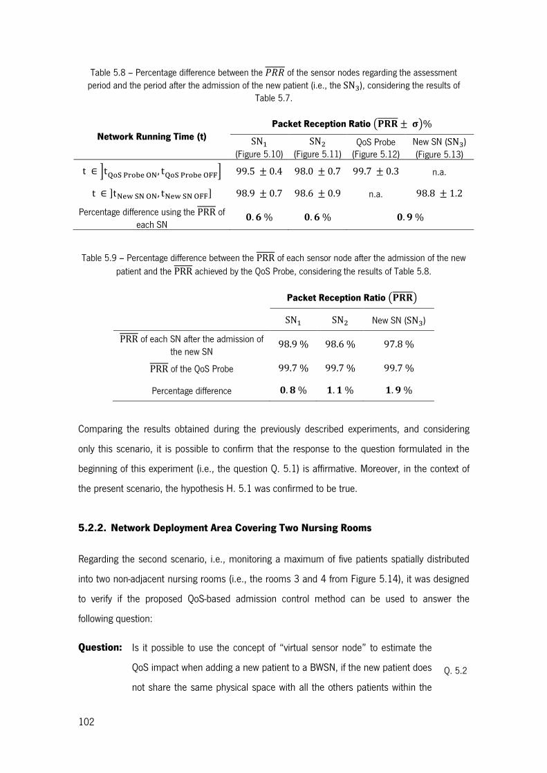
102

Table 5.8 – Percentage difference between the �� of the sensor nodes regarding the assessment period and the period after the admission of the new patient (i.e., theSNº), considering the results of

Table 5.7.


Packet Reception Ratio HÙÚÚ ± ÜI%

SN4 (Figure 5.10)

SN� (Figure 5.11)


New SN (SNº) (Figure 5.13)

t ∈ ÁtÂPÃ²MPÄNÅÆ, tÂPÃ²MPÄNÅÇÇÁ 99.5 ± 0.4 98.0 ± 0.7 99.7 ± 0.3 n.a.

t ∈ ®tÆNÈÃÆÅÆ, tÆNÈÃÆÅÇÇ® 98.9 ± 0.7 98.6 ± 0.9 n.a. 98.8 ± 1.2 Percentage difference using the PRR of

each SN Ï. Ð% Ï. Ð% Ï. Í%

Table 5.9 – Percentage difference between the PRR of each sensor node after the admission of the new patient and the PRR achieved by the QoS Probe, considering the results of Table 5.8.

Packet Reception Ratio HÙÚÚI SN4 SN� New SN (SNº)

PRR of each SN after the admission of the new SN

98.9% 98.6% 97.8%

PRR of the QoS Probe 99.7% 99.7% 99.7%

Percentage difference Ï. Ì% Ô. Ô% Ô. Í%

Comparing the results obtained during the previously described experiments, and considering

only this scenario, it is possible to confirm that the response to the question formulated in the

beginning of this experiment (i.e., the question Q. 5.1) is affirmative. Moreover, in the context of

the present scenario, the hypothesis H. 5.1 was confirmed to be true.

5.2.2. Network Deployment Area Covering Two Nursing Rooms

Regarding the second scenario, i.e., monitoring a maximum of five patients spatially distributed

into two non-adjacent nursing rooms (i.e., the rooms 3 and 4 from Figure 5.14), it was designed

to verify if the proposed QoS-based admission control method can be used to answer the

following question:


QoS impact when adding a new patient to a BWSN, if the new patient does

not share the same physical space with all the others patients within the

Q. 5.2

103

network?

Among all the experiments performed using this scenario, the following two were chosen to be

discussed in order to find the response to the question Q. 5.2.

5.2.2.1. Using different data paths to route the data to the sink

This experiment comprises a BWSN being used to monitor three patients (i.e., the ��4 and the �� in the room 3 and the ��º in the room 4), see the Figure 5.14 and the Table 5.10 for additional information about the network topology.

Figure 5.14 – BWSN used to monitor four patients distributed by two non-adjacent rooms (i.e., the rooms 3 and 4). Table 5.10 shows the sink’s routing table regarding this network topology.



Node ID: Node IP: Node ID: Node IP: ��4 AAAA::0212:7400:13CA:EDE2 ��4 FE80::0212:7400:13CA:EDE2 �� AAAA::0212:7400:13CB:45D9 ��4 AAAA::0212:7400:13CA:EDE2 ��4 AAAA::0212:7400:13CA:E837 �� AAAA::0212:7400:13CB:45D9 �� AAAA::0212:7400:13CA:FDCA �� AAAA::0212:7400:13CB:45D9 ��º AAAA::0212:7400:13CB:2128 ��4 AAAA::0212:7400:13CA:EDE2 ��Ý AAAA::0212:7400:13CC:3930 ��Ý FE80::0212:7400:13CC:3930

104

Using the proposed QoS-based admission control method, the network was tested to assess the

impact of placing a new patient being monitored into the room 4 (i.e., the ��Ý), in the QoS being provided by the BWSN. In such experiment, both the ��4 and the �� send their data to the sink through the �� and the ��4, while the ��º uses the ��4 to forward its data to the sink (see the Figure 5.14 and the Table 5.10 for more details). During the network assessment

period, the QoS Probe sends its data using the same path as the ��º. On the contrary, the new sensor node (i.e., the ��Ý) sends its data directly to the sink. By using different paths to send their data to the sink, it is expectable that the impact of adding the QoS Probe and the new

sensor node in the QoS being provided by the network will be distinct. Moreover it is expected

that the PRR achieved by the QoS Probe will be different from the one achieved by the new

sensor node.

Table 5.11 shows the results obtained when assessing the proposed QoS-based admission

control method, using the experiment presented in the Figure 5.14. In view of those results, it is

possible to state that during both the assessment period using the QoS Probe (i.e., t ∈ÁtÂPÃ²MPÄNÅÆ, tÂPÃ²MPÄNÅÇÇÁ) and the period after introducing the new sensor node (i.e., t ∈ ®tÆNÈÃÆÅÆ, tÆNÈÃÆÅÇÇ®), the network’s performance decrease substantially. However, the performance loss is considerably smaller when introducing the new sensor node. This

behaviour was expected since the data generated by both the QoS Probe and the new sensor

node follow different paths to reach the sink.

105

Table 5.11 – Results obtained when assessing the BWSN

, considering the network topology presented in the Figure 5.14.


Packet Reception Ratio HÉ�

�±Ë I%

�� 4

(Figure 5.15)

��

(Figure 5.16)

�� º

(Figure 5.17)

QoS Probe

(Figure 5.18)

New

SN (�� Ý

)

(Figure 5.19)

t∈Á0,t

ÂPÃ²MP

ÄNÅÆÁ

97.9±1

.6 98.1

±1.4

97.7±1

.6 n.a.

n.a.

t∈Át ÂP

Ã²MPÄN

ÅÆ,t ÂP

Ã²MPÄN

ÅÇÇÁ

ÌÎ.Ð±

Î.Î

ÌÎ.Ì±

Î.Ì

ÌÐ.Í±

Î.Ñ

ÌÒ.Ò±

Î.Ï

n.a.

t∈Át ÂP

Ã²MPÄN

ÅÇÇ,t Æ

NÈÃÆ

ÅÆÁ

98.0±1

.3 97.4

±2.8

98.6±2

.1 n.a.

n.a.

t∈® t ÆN

ÈÃÆÅ

Æ,t ÆNÈ

ÃÆÅÇÇ

® Í�.

Í±�.Ï

Í�.

Ï±�.Î

ÍÍ.

Î±Ï.Í

n.a.

ÍÑ.Ñ±

Ô.Ò

106

Figure 5.15 – PRR of the data flow generated by the ��4 during the admission control procedure regarding the network topology presented in the Figure 5.14.

Figure 5.16 – PRR of the data flow generated by the �� during the admission control procedure

regarding the network topology presented in the Figure 5.14.

Analysing the performance of each sensor node individually, it is possible to see that the PRR of

both the SN4 and the SN� are identical (see the Figure 5.15 and the Figure 5.16 respectively). In particular, when starting the network assessment using the QoS Probe, the PRR drops from

about 97.9% to 84.6% in the SN4 and from about 98.1% to 84.8% in the SN�, which corresponds to a difference of about 13.3pp for both sensor nodes. On its turn, after the introduction of the new sensor node, the �� drops from about 98% to 92.9% in the ��4 and from about 97.4% to 82% in the ��, which corresponds to a difference of about 5.1pp for the ��4 and of about 5.4pp for the ��. Considering these results it is possible do conclude that the performance degradation in the �� of both the ��4 and the �� is approximately ½ after the introduction of the new sensor node when comparing with the one

achieved during the QoS Probe operation. This difference can be explained by the distinct data

paths used by the QoS Probe and by the new sensor node to send their data to the sink. By

107

selecting a distinct path to send its data to the sink, the new sensor node does not contribute to

congest the data path being used by the others sensor nodes and, consequently, its interference

in the performance of those sensor nodes is reduced when compared with the one introduced by

the QoS Probe.

Regarding the performance of the ��º, its �� falls from about 97.7% to 86.9% (i.e.,

dropping about 10.8pp) when starting the assessment period using the QoS Probe and slightly increases after the introduction of the new sensor node in the network, from about 98.6% to

99.4% (i.e., rising about 0.8pp), see the Figure 5.17. Once again, this comportment can be explained by the different paths used by the QoS Probe and by the new sensor node to send their

data to the sink. By using a different and uncongested path to send its data to the sink, the

interferences caused by the new sensor node are highly reduced. Moreover, the distance

between the ��º and the sink is two hops; on its turn, the distance between the ��4 or the �� and the sink is three hops. This difference in the distance between these sensor nodes and the

sink helps to justify the difference in the performance of the ��º when comparing with both the ��4 and the ��. Indeed, the smaller the number of hops between two sensor nodes the higher the PRR.

Figure 5.17 – PRR of the data flow generated by the ��º during the admission control procedure regarding the network topology presented in the Figure 5.14.

Figure 5.18 shows the PRR of the data flow generated by the QoS Probe. During the QoS Probe

operation, the PRR associated with its data flow was of about 87.7%. On its turn, the �� of the data flow generated by the new sensor node was of about 95.5%, see Figure 5.19. By using

a different and uncongested path to send its data to the sink the new sensor node has a higher

probability of successfully deliver its data when compared with the QoS Probe.

108

Figure 5.18 – PRR of the data flow generated by the QoS Probe during the admission control procedure regarding the network topology presented in the Figure 5.14.

Figure 5.19 – PRR of the data flow generated by the new sensor node (i.e., the ��Ý) during the admission control procedure regarding the network topology presented in the Figure 5.14.

Comparing the performance of the sensor nodes within the network during the assessment

period (i.e., t ∈ ÁtÂPÃ²MPÄNÅÆ, tÂPÃ²MPÄNÅÇÇÁ) and the period after the admission of the new sensor node to the network (i.e., t ∈ ®tÆNÈÃÆÅÆ, tÆNÈÃÆÅÇÇ®) using the percentage difference as defined in Eq. 5.2, it is possible to confirm that the QoS Probe and the new sensor

node affect the network performance in distinct ways, as expected. See the Table 5.12 for more

details. Moreover, comparing the performance achieved by each sensor node with the one

achieved by the QoS Probe, as shown in the Table 5.13, it is possible to verify that they are

considerably different. Consequently, considering this scenario and this particular experiment, as

described in the Figure 5.14, the proposed QoS-Based admission control method was unable to

predict the network’s performance after the admission of the new sensor node. In this case, the

answer to the question Q. 5.2 is negative and the hypothesis H. 5.1 is considered to be false.

109

Table 5.12 – Percentage difference between the ��

of the sensor nodes regarding the assessment period and the period after the admission of the new

patient (i.e.,

theSN

Ý), considering the results of Table 5.11.



�±Ë I%

�� 4

(Figure 5.15)

��

(Figure 5.16)

�� º

(Figure 5.17)

QoS Probe

(Figure 5.18)

New

SN (�� Ý

)

(Figure 5.19)

t∈Át ÂP

Ã²MPÄN

ÅÆ,t ÂP

Ã²MPÄN

ÅÇÇÁ

ÌÎ.Ð±

Î.Î

ÌÎ.Ì±

Î.Ì

ÌÐ.Í±

Î.Ñ

ÌÒ.Ò±

Î.Ï

n.a.

t∈® t ÆN

ÈÃÆÅ

Æ,t ÆNÈ

ÃÆÅÇÇ

® Í�.

Í±�.Ï

Í�.

Ï±�.Î

ÍÍ.

Î±Ï.Í

n.a.

ÍÑ.Ñ±

Ô.Ò

Percentage difference using the PRR

of each SN

Í.Î

% Ì.Ô

% ÔÓ.

Î%

Ì.Ñ%

110


Packet Reception Ratio HÙÚÚI

SN4 SN� SNº NewSN"SNÝ$PRR of each SN after the admission of

the new SN 92.9% 92% 99.4% 95.5%

PRR of the QoS Probe 87.7% 87.7% 87.7% 87.7%

Percentage difference Ñ. Ì% Î. Ì% Ô�. Ñ% Ì. Ñ%

5.2.2.2. Using the same data path to route the data to the sink

Regarding this experiment, the ��4 sends its data to the sink through the �� while the remaining sensor nodes, including the QoS Probe and the new sensor node (i.e., the ��Ý), use the ��4 to forward their data packets to the sink (see the Figure 5.14 and the Table 5.10 for more details). In this case, the data generated by the QoS Probe and by the new sensor node

follow the same path to reach the sink. Unlike the former experiment, in this case it is likely that

the QoS Probe and the new sensor node achieve comparable performance in terms of PRR. The

results obtained when assessing the current scenario, using the network topology pictured in the

Figure 5.20 and explained in detail in the Table 5.14, are summarized in the Table 5.15.

Figure 5.20 – BWSN used to monitor five patients distributed by two non-adjacent rooms (i.e., the rooms

3 and 4). Table 5.14 shows the sink’s routing table regarding this network topology.

111



Node ID: Node IP: Node ID: Node IP: ��4 AAAA::0212:7400:13CB:2777 ��4 FE80::0212:7400:13CB:2777 �� AAAA::0212:7400:13CC:392F �� FE80::0212:7400:13CC:392F ��4 AAAA::0212:7400:13CB:3050 �� AAAA::0212:7400:13CC:392F �� AAAA::0212:7400:13CB:3F66 ��4 AAAA::0212:7400:13CB:2777 ��º AAAA::0212:7400:13CA:FDCA ��4 AAAA::0212:7400:13CB:2777 ��Ý AAAA::0212:7400:13CA:E837 ��4 AAAA::0212:7400:13CB:2777 ��¼ AAAA::0212:7400:13CB:2128 ��4 AAAA::0212:7400:13CB:2777

Considering the results presented in the Table 5.15, it is possible to verify that during both the

assessment period using the QoS Probe and the period next to the introduction of the new sensor

node, the network’s performance suffers a significant degradation. Moreover, it is important to

notice that the performance degradation experienced by all the sensor nodes inside the room 4 is

comparable, including the QoS Probe and the new sensor node (i.e., the ��¼). This outcome was expected since the data generated both by the QoS Probe and by the ��¼ use the same path to reach the sink. By using the same data path, it is expected that both have the

comparable impact on the performance of the sensor nodes on their neighbouring (i.e., inside

the room 4).

Taking a look at the individual performance of each sensor node, it is possible to verify that the

PRRs achieved by both the ��4 (Figure 5.21) and the �� (Figure 5.22) during this experiment are comparable. Namely, when starting the QoS Probe, the �� drops from about 83.9% to

57.1% in the ��4 and from about 83.5% to 57.1% in the��, corresponding to a difference of about 26.8pp and 26.4pp, respectively. On its turn, after adding the new sensor node to the network, the �� drops from about 86.8% to 64.5% in the ��4 and from about 86.3% to 65.1% in the ��, corresponding to a difference of about 22.3pp and 21.2pp, respectively. Comparing these results it is possible to verify that the �� of both sensor nodes suffers a greater degradation during the QoS Probe operation, rather than after the addition of the

new sensor node to the network. Although, despite the PRR achieved during the new sensor node

operation have been greater than the one achieved during the QoS Probe operation, it is possible

to conclude that in both cases the performance of these sensor nodes worsens considerably.

112





�±Ë I%

�� 4

(Figure 5.21

)

��

(Figure 5.22

)

�� º

(Figure 5.23

)

�� Ý

(Figure 5.24

) QoS Probe

(Figure 5.25

) New

SN (�� ¼

)

(Figure 5.26

)

t∈Á0,t

ÂPÃ²MP

ÄNÅÆÁ

83.9±4

.4 83.5

±4.1

86.2±3

.1 86.3

±3.3

n.a

n.a

t∈Át ÂP

Ã²MPÄN

ÅÆ,t ÂP

Ã²MPÄN

ÅÇÇÁ

ÑÒ.Ô±

Ò.Ó

ÑÒ.Ô±

Ò.Ó

ÐÓ.Ñ±

Í.Ñ

ÐÑ.Ò±

Ò.Ò

ÐÓ.Ò±

Ð.Ò

n.a

t∈Át ÂP

Ã²MPÄN

ÅÇÇ,t Æ

NÈÃÆ

ÅÆÁ

86.8±2

.5 86.3

±3.2

82.5±8

.4 80.6

±8.8

n.a

n.a

t∈® t ÆN

ÈÃÆÅ

Æ,t ÆNÈ

ÃÆÅÇÇ

® ÐÎ.

Ñ±Ò.Ï

ÐÑ.

Ô±Ì.Ñ

ÐÐ.

Í±Í.Ð

ÐÒ.

Ô±Ì.Ó

n.a

ÐÑ.Í±

Ð.Ì

113


Figure 5.22 – PRR of the data flow generated by the �� during the admission control procedure regarding the network topology presented in the Figure 5.20.

Vis-à-vis the performance of the sensor nodes within the room 4 (i.e., the ��º and the ��Ý) their PRR can be seen in the Figure 5.23 and Figure 5.24, respectively. Once again, the ��[ accomplished by both sensor nodes during this experiment are comparable. Regarding the �� of the ��º, it drops from about 86.2% to 63.5% when starting the QoS Probe operation and

drops from about 82.5% to 66.9% once adding the new sensor node to the network, which

corresponds to a variance of about 22.7pp and 15.6pp, respectively. Considering the �� of the ��Ý, it drops from about 86.3% to 65.7% when starting the assessment with the QoS

Probe and drops from about 80.6% to 67.1% when adding the new sensor node to the

network, which corresponds to a difference of about 20.6pp and 13.5pp, respectively. Taking these results into account, it is possible to verify that the performance degradation introduced by

the QoS Probe is greater than the one introduced by the new sensor node, although, both results

are comparable. This can be explained by the fact that both the QoS Probe and the new sensor

114

node send their data to the sink through the same path. So, as expected, their impact in the

performance of both the ��º and the ��Ý is equivalent.

Figure 5.23 – PRR of the data flow generated by the ��º during the admission control procedure regarding the network topology presented in the Figure 5.20.

Figure 5.24 – PRR of the data flow generated by the ��Ý during the admission control procedure regarding the network topology presented in the Figure 5.20.

Regarding the performance of the QoS Probe, the Figure 5.25 shows its PRR. During the QoS

Probe operation period, the �� achieved by its data flow was of about 63.7%. On its turn, the

Figure 5.26 shows the PRR associated with the data flow generated by the new sensor node (i.e.,

the ��¼) and its �� was of about 65.9%. As expected, the �� of both the QoS Probe and the new sensor node are similar. By using the same path to route their data packets to the sink it

was expected that both reach similar values of PRR.

115



Figure 5.26 – PRR of the data flow generated by the new sensor node (i.e., the ��¼) during the admission

control procedure regarding the network topology presented in the Figure 5.20.

Comparing the PRR of all the sensor nodes within the network during the network assessment period (i.e., t ∈ ÁtÂPÃ²MPÄNÅÆ, tÂPÃ²MPÄNÅÇÇÁ) and the period after the admission of the new sensor node to the network (i.e., t ∈ ®tÆNÈÃÆÅÆ, tÆNÈÃÆÅÇÇ®) using the percentage difference as defined in Eq. 5.2, it is possible to conclude that both the QoS Probe and the new

sensor node affect the sensor nodes within the network distinctly. In fact, looking to the results of

the Table 5.16 it is clear that the performance of the sensor nodes inside the room 3 (i.e., the

SN4 and the SN�) are distinctly affected by the QoS Probe and by the new sensor node. Nevertheless, the sensor nodes inside the room 4 (i.e., the SNº and the SNÝ) have seen their performance affected in a comparable way by the QoS Probe and by the new sensor node.

Moreover, when comparing the PRR achieved by each sensor node within the network, including the new one, with the PRR achieved by the QoS Probe during its operation, it is possible to verify that the PRR of all the sensor nodes after the admission of the new sensor node is comparable with the one achieved by the QoS Probe, as presented in the Table 5.17. In view of these results

it is possible to argue that the proposed method was able to predict the impact of adding the new

node to the network.

116



patient

(i.e., theSN ¼

), considering the results of Table 5.15.



�±Ë I%

�� 4

(Figure 5.21

)

��

(Figure 5.22

)

�� º

(Figure 5.23

)

�� Ý

(Figure 5.24

) QoS Probe

(Figure 5.25

) New

SN (�� ¼

)

(Figure 5.26

)

t∈Át ÂP

Ã²MPÄN

ÅÆ,t ÂP

Ã²MPÄN

ÅÇÇÁ

ÑÒ.Ô±

Ò.Ó

ÑÒ.Ô±

Ò.Ó

ÐÓ.Ñ±

Í.Ñ

ÐÑ.Ò±

Ò.Ò ÐÓ.

Ò±Ð.Ò

n.a

t∈® t ÆN

ÈÃÆÅ

Æ,t ÆNÈ

ÃÆÅÇÇ

® ÐÎ.

Ñ±Ò.Ï

ÐÑ.

Ô±Ì.Ñ

ÐÐ.

Í±Í.Ð

ÐÒ.

Ô±Ì.Ó

n.a

ÐÑ.Í±

Ð.Ì

Percentage difference using the PRR

of each SN

Ô�.

�%

ÔÓ.Ô%

Ñ.�

% �.Ô

% Ó.Î

%

117



SN4 SN� SNº SNÝ NewSN"SN¼$ PRR of each SN after the admission of the new SN

64.5% 65.1% 66.9% 67.1% 65.9%

PRR of the QoS Probe 63.7% 63.7% 63.7% 63.7% 63.7%

Percentage difference Ô. �% �. �% Î. Í% Ñ. �% Ó. Î%

Regarding the results obtained during the aforementioned experiments, and considering only this

scenario, it is possible to claim that the proposed QoS-based admission control method was able

to predict the impact of adding the new patient to the network only in the experiment pictured in

the Figure 5.20. So, the response to the question Q. 5.2 is affirmative only in that case.

Consequently, the hypothesis H. 5.1 is considered to be true only for that experiment.

5.2.3. Network Deployment Area Covering Three Nursing Rooms

This scenario is about monitoring a maximum of five patients distributed by three rooms (i.e., the

rooms 3, 4, and 5 from the Figure 5.27). This scenario was designed to evaluate the impact of

the building structure when assessing the BWSN using the proposed method and in view of the

results achieved respond to the following question:


QoS impact when adding a new patient to a BWSN, when the new patient

does not share the same physical space with all the others patients within

the network neither with the “virtual sensor node”?

Q. 5.3

This scenario involves four patients being monitored while sharing two non-adjacent rooms. More

precisely, the SN4 and the SN� inside the room 3, and the SNº and the SNÝ inside the room 4, as pictured in the Figure 5.27. Then, the suggested QoS-based admission control method is used

to evaluate if a new patient (i.e., the SN¼) can be added to the BWSN inside the room 5, see Figure 5.27. At the end of the assessment period, the decision of adding the new patient in room

5 is made facing the results obtained.

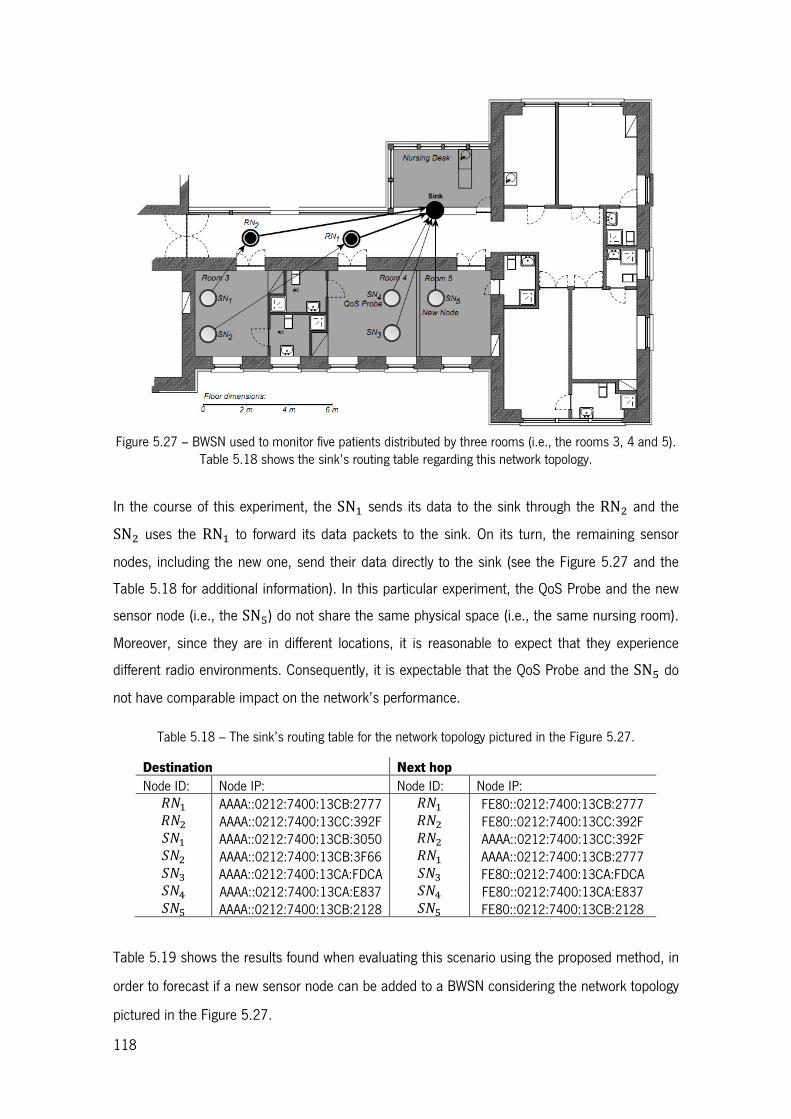
118

Figure 5.27 – BWSN used to monitor five patients distributed by three rooms (i.e., the rooms 3, 4 and 5).

Table 5.18 shows the sink’s routing table regarding this network topology.

In the course of this experiment, the SN4 sends its data to the sink through the RN� and the SN� uses the RN4 to forward its data packets to the sink. On its turn, the remaining sensor nodes, including the new one, send their data directly to the sink (see the Figure 5.27 and the

Table 5.18 for additional information). In this particular experiment, the QoS Probe and the new

sensor node (i.e., the SN¼) do not share the same physical space (i.e., the same nursing room). Moreover, since they are in different locations, it is reasonable to expect that they experience

different radio environments. Consequently, it is expectable that the QoS Probe and the SN¼ do not have comparable impact on the network’s performance.



Node ID: Node IP: Node ID: Node IP: ��4 AAAA::0212:7400:13CB:2777 ��4 FE80::0212:7400:13CB:2777 �� AAAA::0212:7400:13CC:392F �� FE80::0212:7400:13CC:392F ��4 AAAA::0212:7400:13CB:3050 �� AAAA::0212:7400:13CC:392F �� AAAA::0212:7400:13CB:3F66 ��4 AAAA::0212:7400:13CB:2777 ��º AAAA::0212:7400:13CA:FDCA ��º FE80::0212:7400:13CA:FDCA ��Ý AAAA::0212:7400:13CA:E837 ��Ý FE80::0212:7400:13CA:E837 ��¼ AAAA::0212:7400:13CB:2128 ��¼ FE80::0212:7400:13CB:2128

Table 5.19 shows the results found when evaluating this scenario using the proposed method, in

order to forecast if a new sensor node can be added to a BWSN considering the network topology

pictured in the Figure 5.27.

119





�±ËI

% �� 4

(Figure 5.28

)

��

(Figure 5.29

)

�� º

(Figure 5.30

)

�� Ý

(Figure 5.31

) QoS Probe

(Figure 5.32

) New

SN (�� ¼

)

(Figure 5.33

)

t∈Á0,t

ÂPÃ²MP

ÄNÅÆÁ

97.3±2

.3 97.7

±1.9

98.0±0

.8 97.7

±1.0

n.a

n.a

t∈Át ÂP

Ã²MPÄN

ÅÆ,t ÂP

Ã²MPÄN

ÅÇÇÁ

ÍÒ.Ó±

Ó.Ô

ÍÒ.Í±

�.Î

ÍÔ.Ô±

Ô.Ñ

ÍÏ.Ì±

Ô.Ì Í�.

Ï±�.Ï

n.a

t∈Át ÂP

Ã²MPÄN

ÅÇÇ,t Æ

NÈÃÆ

ÅÆÁ

95.5±2

.2 95.2

±2.6

94.9±1

.9 94.3

±1.9

n.a

n.a

t∈® t ÆN

ÈÃÆÅ

Æ,t ÆNÈ

ÃÆÅÇÇ

® ÍÐ.

Ì±�.Ó

ÍÐ.

Ô±�.Ì

ÌÑ.

Ð±Ó.Î

Ì�.

Ò±Ó.Ò

n.a

ÌÑ.Ô±

�.Î

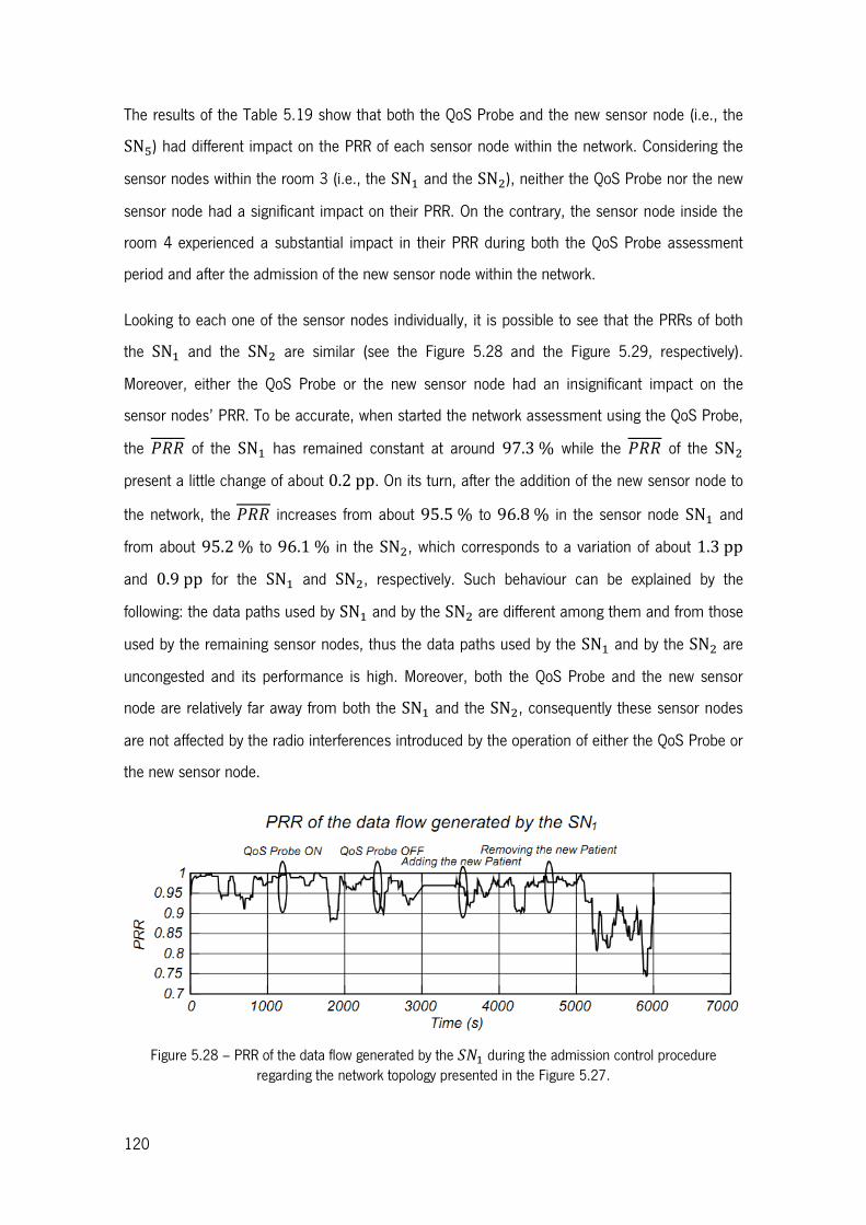
120

The results of the Table 5.19 show that both the QoS Probe and the new sensor node (i.e., the

SN¼) had different impact on the PRR of each sensor node within the network. Considering the sensor nodes within the room 3 (i.e., the SN4 and the SN�), neither the QoS Probe nor the new sensor node had a significant impact on their PRR. On the contrary, the sensor node inside the

room 4 experienced a substantial impact in their PRR during both the QoS Probe assessment

period and after the admission of the new sensor node within the network.

Looking to each one of the sensor nodes individually, it is possible to see that the PRRs of both

the SN4 and the SN� are similar (see the Figure 5.28 and the Figure 5.29, respectively). Moreover, either the QoS Probe or the new sensor node had an insignificant impact on the

sensor nodes’ PRR. To be accurate, when started the network assessment using the QoS Probe,

the �� of the SN4 has remained constant at around 97.3% while the �� of the SN� present a little change of about 0.2pp. On its turn, after the addition of the new sensor node to the network, the �� increases from about 95.5% to 96.8% in the sensor node SN4 and from about 95.2% to 96.1% in the SN�, which corresponds to a variation of about 1.3pp and 0.9pp for the SN4 and SN�, respectively. Such behaviour can be explained by the following: the data paths used by SN4 and by the SN� are different among them and from those used by the remaining sensor nodes, thus the data paths used by the SN4 and by the SN� are uncongested and its performance is high. Moreover, both the QoS Probe and the new sensor

node are relatively far away from both the SN4 and the SN�, consequently these sensor nodes are not affected by the radio interferences introduced by the operation of either the QoS Probe or

the new sensor node.


121

Figure 5.29 – PRR of the data flow generated by the �� during the admission control procedure regarding the network topology presented in the Figure 5.27.

Considering the sensor nodes inside the nursing room 4, the PRR achieved by both the SNº and the SNÝ are pictured in the Figure 5.30 and the Figure 5.31, respectively. Analysing both PRRs, it is possible to conclude that they achieve comparable rates and have a similar behaviour. To be

accurate, the �� of the SNº falls from about 98.0% to 91.1% and the �� of the SNÝ falls from about 97.7% to 90.8%, when the QoS Probe starts its operation which corresponds

to a variation of about 6.9pp for both the SNº and the SNÝ. On its turn, when the new sensor node is added to the network, the �� of the SNº falls from about 94.9% to 85.6% and the

�� of the SNÝ falls from about 94.3% to 82.7%, which corresponds to a variation of about

9.3pp for the SNº and of about 11.6pp for the SNÝ. The SNº and the SNÝ share the same physical space with the QoS Probe, in this way the QoS Probe could have a significant impact in

their radio environment, and contribute to a degradation on their PRR. Moreover, the QoS Probe

also shares the same data path with both the SNº and the SNÝ, consequently this data path becomes more congested, contributing to the degradation of the PRR of all the nodes using it. On

its turn, the new sensor node does not share the same room with the remaining sensor nodes.

However, it is close enough to introduce significant interferences in the radio environment of the

sensor nodes within the room 4. In this way, such interferences could justify part of the

degradation experienced by both the SNº and the SNÝ. Regarding the data path used by the new sensor node, it is directly connected to the sink as both the SNº and the SNÝ are. As before, the new sensor node increases the occupation rate of the wireless link and the performance of the

sensor nodes using it can decrease substantially.

122

Figure 5.30 – PRR of the data flow generated by the ��º during the admission control procedure


Figure 5.31 – PRR of the data flow generated by the ��Ý during the admission control procedure


Figure 5.32 shows the PRR of the data flow produced by the QoS Probe. During the QoS Probe

operation, the �� associated with its data flow was of about 92%. On its turn, the �� of the data flow produced by the new sensor node (i.e., SN¼) was of about 85.1% (see the Figure

5.33). Since the QoS Probe and the new sensor node do not share the same nursing room, they

are under different radio conditions. Thus, it is expectable that they reach different PRRs.



123

Figure 5.33 – PRR of the data flow generated by the new sensor node (i.e., the ��¼) during the admission

control procedure regarding the network topology presented in the Figure 5.27.

Comparing the PRR of each one of the sensor nodes within the network during the QoS Probe operation (i.e., t ∈ ÁtÂPÃ²MPÄNÅÆ, tÂPÃ²MPÄNÅÇÇÁ) and after the addition of the new sensor node (i.e., t ∈ ®tÆNÈÃÆÅÆ, tÆNÈÃÆÅÇÇ®) using the percentage difference as defined in Eq. 5.2, it is possible to argue that the QoS Probe and the new sensor node (i.e., ��¼) affect the PRR of the sensor nodes within the network in different ways. Indeed, looking to the results

presented in the Table 5.20 it becomes clear that the PRR of the sensor nodes inside the nursing

room 3 (i.e., the SN4 and the SN�) is not affected neither by the QoS Probe nor by the new sensor node. On its turn, the sensor nodes within the nursing room 4 (i.e., the SNº and the SNÝ) are significantly affected either by the QoS Probe and by the new sensor node; however, they are

affected differently. In fact, the difference on the �� achieved by the SNº and by the SNÝ during the QoS Probe operation and the period after adding the new sensor node is of about

6.2% and 9.3%, respectively. Moreover, the �� achieved by the QoS Prove is not comparable with the one achieved by the new sensor node (see Table 5.20). Comparing the

�� of each sensor node after adding the new sensor node to the network, with the �� achieved by the QoS Probe, it is not comparable for most of the sensor nodes (see Table 5.21).

In fact, for those outside the room 3 (i.e., the SNº, the SNÝ, the SN¼ and the QoS Probe) the difference in the �� achieved during those two periods is of about 6.2%, 9.3% and 7.8%

for the SNº, SNÝ and SN¼, respectively. Taking into consideration these results, it is possible to argue that the proposed admission control method was unable to predict the impact of adding

the new sensor node to the network.

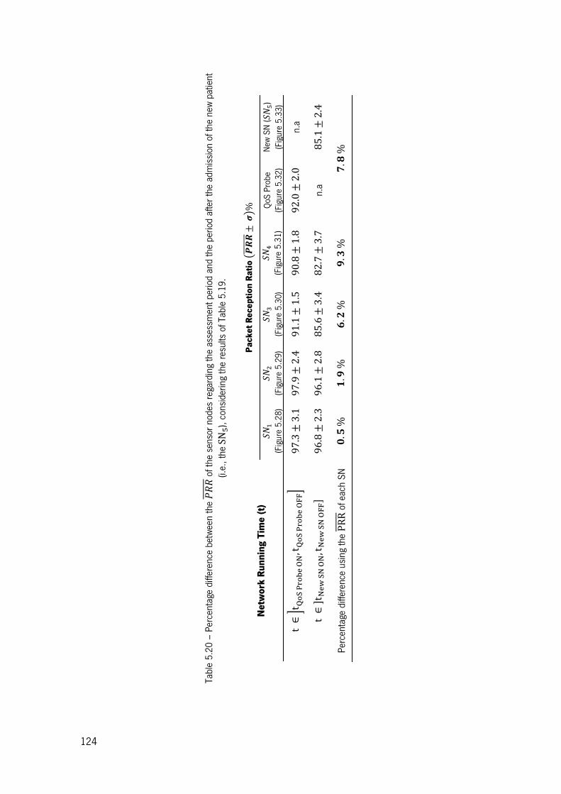
124



patient

(i.e., theSN ¼

), considering the results of Table 5.19.



�±ËI%

�� 4

(Figure 5.28

)

��

(Figure 5.29

)

�� º

(Figure 5.30

)

�� Ý

(Figure 5.31

) QoS Probe

(Figure 5.32

) New

SN (�� ¼

)

(Figure 5.33

)

t∈Át ÂP

Ã²MPÄN

ÅÆ,t ÂP

Ã²MPÄN

ÅÇÇÁ

97.3±3

.1 97.9

±2.4

91.1±1

.5 90.8

±1.8

92.0±2

.0 n.a

t∈® t ÆN

ÈÃÆÅ

Æ,t ÆNÈ

ÃÆÅÇÇ

® 96.8

±2.3

96.1±2

.8 85.6

±3.4

82.7±3

.7 n.a

85.1±2

.4Percentage difference using the PRR

of each SN

Ï.Ñ

% Ô.Í

% Ð.�

% Í.Ó

% Ò.Ì

%

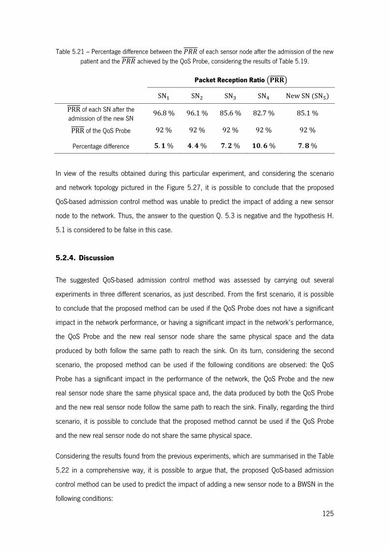
125



SN4 SN� SNº SNÝ NewSN"SN¼$ PRR of each SN after the admission of the new SN

96.8% 96.1% 85.6% 82.7% 85.1%

PRR of the QoS Probe 92% 92% 92% 92% 92%

Percentage difference Ñ. Ô% Î. Î% Ò. �% ÔÏ. Ð% Ò. Ì%

In view of the results obtained during this particular experiment, and considering the scenario

and network topology pictured in the Figure 5.27, it is possible to conclude that the proposed

QoS-based admission control method was unable to predict the impact of adding a new sensor

node to the network. Thus, the answer to the question Q. 5.3 is negative and the hypothesis H.

5.1 is considered to be false in this case.

5.2.4. Discussion

The suggested QoS-based admission control method was assessed by carrying out several

experiments in three different scenarios, as just described. From the first scenario, it is possible

to conclude that the proposed method can be used if the QoS Probe does not have a significant

impact in the network performance, or having a significant impact in the network’s performance,

the QoS Probe and the new real sensor node share the same physical space and the data

produced by both follow the same path to reach the sink. On its turn, considering the second

scenario, the proposed method can be used if the following conditions are observed: the QoS

Probe has a significant impact in the performance of the network, the QoS Probe and the new

real sensor node share the same physical space and, the data produced by both the QoS Probe

and the new real sensor node follow the same path to reach the sink. Finally, regarding the third

scenario, it is possible to conclude that the proposed method cannot be used if the QoS Probe

and the new real sensor node do not share the same physical space.

Considering the results found from the previous experiments, which are summarised in the Table

5.22 in a comprehensive way, it is possible to argue that, the proposed QoS-based admission

control method can be used to predict the impact of adding a new sensor node to a BWSN in the

following conditions:

126

1. The “virtual sensor node” and the new real sensor node have to share the same physical

space;

2. The data produced by both the “virtual sensor node” and the new real sensor node,

must follow the same path to reach the sink.

Table 5.22 – Results summary in view of the evaluation of the proposed admission control method.

Network Covering

One Room

Network Covering

Two Rooms

Network

Covering

Three Rooms

Using the same data

path

Using different data paths

Using different data paths

Using the same data

path Using different data paths

Do the QoS Probe and the new sensor node share the same physical space?

Yes Yes Yes Yes No

Do the data produced by the QoS Probe and by the new sensor node follow the same path to the sink?

Yes No No Yes Yes

Has the QoS Probe a significant impact on the network performance?

Yes No Yes Yes Yes

Have the QoS Probe and the new sensor node a comparable impact on the network performance, and is the hypothesis H. 5.1 true?

Yes Yes No Yes No

5.3. Summary

This chapter described the real-world tests made to assess the QoS-based admission control

module proposed. First, the detailed study made to understand the network deployment

environment and its characteristics, as well as the initial network deployment, were explained in

detail. Then, the experiments performed to assess the QoS-based admission control modules

were explained and analysed in detail. Those experiments were made in three distinct scenarios,

comprising several network topologies. Finally, in view of the results obtained, significant

conclusions were drawn. In particular, were identified the conditions in which the proposed

QoS-based admission control method can be employed.

127

Chapter 6

Conclusions and Future Work

Key Findings and Promising Directions

6.1. Conclusions

6.2. Future work

129

6. Conclusions and Future Work

This chapter condenses the motivation, objectives, contributions and conclusions of this thesis. It

also suggests promising directions for future research.

6.1. Conclusions

Wireless sensor networks combined with low-power sensor devices, have the potential to

integrate the physical world with wildly used computing systems. Furthermore, such networks

can be used to create ubiquitous and pervasive intelligent systems with the potential to greatly

impact our daily lives. Among all the application areas of the wireless sensor network, the

healthcare is one of the most promising. In particular, concerning its potential to change not only

the today’s healthcare services provided to the citizens but also the clinical practice. The use of

WSNs in healthcare brings several advantages, in particular as regards to the automation of

routine processes such as periodic patient monitoring. Automatic patient monitoring systems can

be used to complement the episodic measurements made by the healthcare professionals (e.g.,

body temperature, pulse and respiratory rates, blood pressure or oximetry), bringing out an

enhancement of the quality of care, while freeing the nursing staff to provide extra attention to the

patients.

Nevertheless, due to the demanding requirements of healthcare services and applications, WSNs

have to fulfil high levels of quality of service (QoS) to be fully accepted by the healthcare

professionals and patients. As an effort to provide healthcare professionals with a tool to manage

such networks, bearing in mind the objective of maximising the QoS provided by WNSs

supporting patient monitoring applications, this thesis proposes a new QoS-based network

management method able to both monitor the effective QoS provided by the network and

manage the admission of new nodes to the network.

The proposed QoS-based network management method consists of two modules, namely the

QoS monitoring module and the QoS-based admission control module. The QoS monitoring

module uses a time-domain mathematical framework to detect and classify potential QoS

degradation events on its very beginning, even before they can worsen the QoS provided by the

network to levels below the limits required by the applications using the WSN. To the best of our

knowledge, this is a distinctive characteristic when comparing the proposed QoS monitoring

130

module with the ones existing on the market, in special, targeting WSNs. By detecting and

classifying potential QoS degradation events on its very beginning, the QoS monitoring module is

able to alert the network administrator to take the necessary measures to ensure the proper

operation of the WSN.

On its turn, the QoS-based admission control module makes use of a “virtual sensor node” to

verify if a new patient (i.e., a new sensor node) can be added to the network and decides which

would be the best place to admit the new patient into the network. The use of a “virtual sensor

node” avoids the necessity of the new patient to be physically present within the network and

enables to assess the on-the-fly QoS provided by the network from a remote location. By using a

“virtual sensor node”, the admission control module enables the network administrator (n.b., the

figure of the network administrator must be seen in a broad sense since it could be either a

person or a virtual process) to estimate the presence of a real sensor node within the network

from a remote location. This characteristic gives the proposed method an innovative feel, when

comparing it with other proposals. Moreover, the possibility to know in advance the best location

to place a patient gives the healthcare providers an important tool to optimise their work and

organizational processes.

The suggested QoS-based network management method was widely tested using both simulated

and real-world environments. Due to its flexibility and facility of use (including the possibility to

repeat the experiments in the exact same conditions), simulated environments were extensively

used in this work, in particular during the development stage. At this point, it was necessary to

choose the network simulator and operating system carefully. The choice has fallen on both the

COOJA network simulator and hardware emulator, and on the Contiki OS. By choosing a network

simulator and hardware emulator, the time to implement real word applications decreases

dramatically since the code used within the simulator environment is the same used in the

real-world applications. Such working method has proven to be effective improving outcomes.

Regarding real-world deployments, they are fundamental to validate and to test the strength of

new solutions. However, such deployments are very hard to manage and control. Indeed, it is

necessary to have a deep knowledge about the deployment area, in particular, regarding the

following aspects: what the obstacles present inside the development area are, if there are other

wireless technologies inside the development area, if there are persons walking around the

development area, or if there are other equipment or machinery able to cause electromagnetic

131

interferences. In other words, it is necessary to study the development area, before the network

deployment, and identify risk factors able to decrease the QoS provided by the network.

The results obtained using both simulated and real environments, have endorsed the QoS-based

proposed QoS-based network management method. In particular, the QoS monitoring module

was validated based on several simulation tests. On its turn, the admission control module and

particularly the concept of “virtual sensor node” were validated using both simulated and

real-world deployments.

The QoS monitoring module was able to detect and classify potential QoS degradation events.

Moreover, by using not only the metrics value but also its behaviour and tendency, the QoS

monitoring module have proved to be able to detect and classify potential QoS degradation

events even before the QoS metric in cause reaches critical values. This ability can be used to

fire warning messages, providing the network administrator with valuable information to prevent

the network malfunction.

Regarding the QoS-based admission control module, it is possible to outcome that the proposed

method, based on the use of a “virtual sensor node” to predict the behaviour of the network

when introducing the new sensor node, was successfully validated under the following conditions:

1. The “virtual sensor node” and the new real sensor node have to share the same physical

space;

2. The data produced by both the “virtual sensor node” and the new real sensor node,

must follow the same path to reach the sink.

In summary, the proposed QoS-based network management method was clearly presented and

validated using different scenarios. Finally, the conditions necessary to its use were clearly

presented.

6.2. Future Work

There are some interesting directions to explore the possibility of developing and implementing

innovative tools using the QoS-based network management method presented in this thesis, one

of which is its implementation using multiple QoS metrics such as, the E2E delay and the delay

variation (i.e., jitter), in addition to the already tested PRR. Managing the network taking into

132

consideration several metrics, improves the network administrator knowledge about the network

behaviour and performance. Being aware of such information is vital to keep the network within

the QoS limits required by the applications using it.

Regarding the concept of “virtual sensor node”, introduced by this thesis, it could be further

improved. In particular, its ability to generate asynchronous data traffic from multiple sensors

considering its statistic properties must be improved. Another aspect regarding the “virtual

sensor node” execution that is worthy of attention is the competition for the hardware resources

existing in the real sensor node, in particular the concurrent assess to the radio interface.

Other important possibility to continue the work presented in this thesis towards the development

of new managing tools, integrating the proposed QoS-based network management method with

existing information and communication systems. Such tools must provide clear and user friendly

interfaces in order to facilitate its use by the healthcare professionals.

133

Appendix A

List of Publications

Patents, Journals, Books, Conferences

Here is a list of publications that reflects the results achieved during the development of these

research work.

Patents

Abreu, C and Mendes, P. Sistema de monitorização de qualidade de serviço e controlo de

admissão em redes de sensores sem fios e respetivo método. Pedido provisório PT 106740.

Journals

Abreu, C.; Ricardo, M.; Mendes, P. Energy-Aware Routing for Biomedical Wireless Sensor

Networks. Journal of Networking and Computer Applications, 40(0), 270-278, 2014.

(Impact Factor: 1.467).

Abreu, C.; Miranda, F.; Ricardo, M.; Mendes, P. QoS-Based Management of Biomedical Wireless

Sensor Networks for Patient Monitoring. In SpringerPlus. 2014. (Publication fee waived!).

Contributions to Books

Abreu, C.; P.M. Mendes, F. Miranda, F. (Ed.). Systems Theory: Perspectives, Applications and Developments. Providing QoS in Wireless Sensor Networks: A System Overview. Nova Science Publishers, Inc., 2014.

Conferences

Abreu, C.; Miranda F.; Mendes, P. Estimating the Impact of Adding Sensor Nodes to Biomedical Wireless Sensor Networks. International Conference of Numerical Analysis and Applied Mathematics 2014 (ICNAAM 2014), Rhodes, Greece, 22-28 September 2014. (Extended Abstract) (Accepted)

Abreu, C.; Mendes, P. End-to-End Quality of Service-Based Admission Control via Virtual Sensor Nodes. In the IFMBE International Conference on Health Informatics. Vilamoura, Algarve, Portugal, 7-9 November 2013.

134

Abreu, C.; Mendes, P. Deployment of Wireless Sensor Networks for Biomedical Applications -- Quality of Service Improvement through Network Lifetime-Extending. In the IEEE 15th International Conference on e-Health Networking, Applications and Services (Healthcom). Lisbon, Portugal, 9-12 October 2013.

Abreu, C.; Mendes, P. Wireless Sensor Networks for Biomedical Applications - Quality of Service, Admission Control and Lifetime-Extending Challenges. In 3rd Portuguese Bioengineering Meeting. Braga, Portugal, 20-22 February 2013.

Abreu, C.; Mendes, P.; Ricardo, M. Framework for QoS Performance Assessment on Biomedical Wireless Sensor Networks. In BIODEVICES2012: International Conference on Biomedical Electronics and Devices. Vilamoura, Algarve, Portugal, 1-4 February 2012. (Short Paper)

Abreu, C.; Mendes, P.; Ricardo, M. Monitoring QoS Over Wireless Sensor Networks: For Medical Applications. In BIODEVICES2011: International Conference on Biomedical Electronics and Electronics and Devices. Rome, Italy, 26-29 January 2011. (Poster)

Invited Paper

Abreu, C.; Mendes, P. Extending Lifetime of Biomedical Wireless Sensor Networks using Energy-aware Routing and Relay Nodes. Submitted to the International Journal of E-Health and Medical Communications.

135

Bibliography

[1] I.F. Akyildiz, Weilian Su, Y. Sankarasubramaniam, and E. Cayirci, "A Survey on Sensor

Networks," Communications Magazine, IEEE, vol. 40, no. 8, pp. 102-114, August 2002.

[2] JeongGil Ko et al., "Wireless Sensor Networks for Healthcare," Proceedings of the IEEE,

vol. 98, no. 11, pp. 1947-1960, November 2010.

[3] Shekhar Borkar and Andrew A. Chien, "The Future of Microprocessors," Commun. ACM,

vol. 54, no. 5, pp. 67-77, May 2011.

[4] Xiaofan Jiang, Joseph Polastre, and David Culler, "Perpetual environmentally powered

sensor networks," in Proceedings of the 4th international symposium on Information

processing in sensor networks, Piscataway, NJ, USA, 2005.

[5] K.J. Vinoy and T.V. Prabhakar, "A Universal Energy Harvesting Scheme for Operating Low-

Power Wireless Sensor Nodes Using Multiple Energy Resources," in Micro and Smart

Devices and Systems, K. J. Vinoy et al., Eds.: Springer India, 2014, pp. 453-466.

[6] Mohamed Younis, Izzet F. Senturk, Kemal Akkaya, Sookyoung Lee, and Fatih Senel,

"Topology management techniques for tolerating node failures in wireless sensor networks:

A survey," Computer Networks , vol. 58, no. 0, pp. 254-283, 2014.

[7] M. Conti and S. Giordano, "Mobile ad hoc networking: milestones, challenges, and new

research directions," Communications Magazine, IEEE, vol. 52, no. 1, pp. 85-96, January

2014.

[8] Hande Alemdar and Cem Ersoy, "Wireless sensor networks for healthcare: A survey,"

Computer Networks, 2010.

[9] Farid Touati and Rohan Tabish, "U-Healthcare System: State-of-the-Art Review and

Challenges," Journal of Medical Systems, vol. 37, no. 3, pp. 1-20, 2013.

[10] Pedro José Marron, Stamatis Karnouskosand Daniel Minder, and Aníbal Ollero, Eds., The

Emerging Domain of Cooperating Objects.: Springer Berlin Heidelberg, 2011.

[11] Jaime Chen, Manuel Díaz, Luis Llopis, Bartolomé Rubio, and José M. Troya, "A survey on

quality of service support in wireless sensor and actor networks: Requirements and

challenges in the context of critical infrastructure protection," Journal of Network and

Computer Applications, vol. 34, no. 4, pp. 1225-1239, 2011, Advanced Topics in Cloud

136

Computing.

[12] Nouha Baccour et al., "Radio link quality estimation in wireless sensor networks: A survey,"

ACM Trans. Sen. Netw., vol. 8, no. 4, pp. 34:1--34:33, Sep. 2012.

[13] S. Pakzad, G. Fenves, S. Kim, and D. Culler, "Design and Implementation of Scalable

Wireless Sensor Network for Structural Monitoring," Journal of Infrastructure Systems, vol.

14, no. 1, pp. 89-101, 2008.

[14] "Systems and software engineering -- Vocabulary," ISO/IEC/IEEE 24765:2010(E), pp. 1-

418, December 2010.

[15] Yanjun Li, Chung Shue Chen, Ye-Qiong Song, and Zhi Wang, "Real-time QoS support in

wireless sensor networks: a survey," in 7th IFAC International Conference on Fieldbuses &

Networks in Industrial & Embedded Systems - FeT2007,

[16] Yinsheng Xu et al., "Real-time Routing in Wireless Sensor Networks: A Potential Field

Approach," ACM Trans. Sen. Netw., vol. 9, no. 3, pp. 35:1--35:24, June 2013.

[17] Jayavardhana Gubbi, Rajkumar Buyya, Slaven Marusic, and Marimuthu Palaniswami,

"Internet of Things (IoT): A vision, architectural elements, and future directions ," Future

Generation Computer Systems , vol. 29, no. 7, pp. 1645-1660, 2013, Including Special

sections: Cyber-enabled Distributed Computing for Ubiquitous Cloud and Network

Services & Cloud Computing and Scientific Applications — Big Data, Scalable Analytics, and

Beyond.

[18] J.M.L.P. Caldeira, J.J.P.C. Rodrigues, and P. Lorenz, "Toward ubiquitous mobility solutions

for body sensor networks on healthcare," Communications Magazine, IEEE, vol. 50, no. 5,

pp. 108-115, 2012.

[19] M. Ali, T. Suleman, and Z.A. Uzmi, "MMAC: a mobility-adaptive, collision-free MAC protocol

for wireless sensor networks," in Performance, Computing, and Communications

Conference, 2005. IPCCC 2005. 24th IEEE International, 2005, pp. 401-407.

[20] Qian Dong and W. Dargie, "A Survey on Mobility and Mobility-Aware MAC Protocols in

Wireless Sensor Networks," Communications Surveys Tutorials, IEEE, vol. 15, no. 1, pp.

88-100, 2013.

[21] Matthias Grossglauser and D.N.C. Tse, "Mobility increases the capacity of ad hoc wireless

networks," Networking, IEEE/ACM Transactions on, vol. 10, no. 4, pp. 477-486, 2002.

[22] GetsyS Sara and D. Sridharan, "Routing in mobile wireless sensor network: a survey,"

Telecommunication Systems, pp. 1-29, 2013.

137

[23] Said Ould Amara, Rachid Beghdad, and Mourad Oussalah, "Securing Wireless Sensor

Networks: A Survey," EDPACS, vol. 47, no. 2, pp. 6-29, 2013.

[24] K. Romer and F. Mattern, "The design space of wireless sensor networks," Wireless

Communications, IEEE, vol. 11, no. 6, pp. 54-61, 2004.

[25] Jeonggil Ko et al., "ContikiRPL and TinyRPL: Happy Together," in Proceedings of the

workshop on Extending the Internet to Low power and Lossy Networks (IPSN 2011),

Chicago, IL, USA, #APR# 2011.

[26] Carlos Abreu, Manuel Ricardo, and P.M. Mendes, "Energy-aware routing for biomedical

wireless sensor networks," Journal of Network and Computer Applications, no. 0, pp. - ,

2013.

[27] Giuseppe Anastasi, Marco Conti, Mario Di Francesco, and Andrea Passarella, "Energy

conservation in wireless sensor networks: A survey," Ad Hoc Networks, vol. 7, no. 3, pp.

537-568, 2009.

[28] Jennifer Yick, Biswanath Mukherjee, and Dipak Ghosal, "Wireless Sensor Network Survey,"

Computer Networks, vol. 52, no. 12, pp. 2292-2330, 2008.

[29] Chonggang Wang, K. Sohraby, Bo Li, M. Daneshmand, and Yueming Hu, "A survey of

transport protocols for wireless sensor networks," Network, IEEE, vol. 20, no. 3, pp. 34-40,

2006.

[30] A. J D Rathnayaka, V.M. Potdar, A. Sharif, S. Sarencheh, and S. Kuruppu, "Wireless Sensor

Network Transport Protocol - A State of the Art," in Broadband, Wireless Computing,

Communication and Applications (BWCCA), 2010 International Conference on, 2010, pp.

812-817.

[31] Y.G. Iyer, S. Gandham, and S. Venkatesan, "STCP: a generic transport layer protocol for

wireless sensor networks," in Computer Communications and Networks, 2005. ICCCN

2005. Proceedings. 14th International Conference on, 2005, pp. 449-454.

[32] Seung-Jong Park, Ramanuja Vedantham, Raghupathy Sivakumar, and Ian F. Akyildiz, "A

Scalable Approach for Reliable Downstream Data Delivery in Wireless Sensor Networks," in

Proceedings of the 5th ACM International Symposium on Mobile Ad Hoc Networking and

Computing, New York, NY, USA, 2004, pp. 78-89.

[33] V.C. Gungor and O.B. Akan, "DST: delay sensitive transport in wireless sensor networks,"

in Computer Networks, 2006 International Symposium on, 2006, pp. 116-122.

[34] Yogesh Sankarasubramaniam, \", and Ian F. Akyildiz, "ESRT: Event-to-sink Reliable

Transport in Wireless Sensor Networks," in Proceedings of the 4th ACM International

138

Symposium on Mobile Ad Hoc Networking \&Amp; Computing, New York, NY, USA, 2003,

pp. 177-188.

[35] F.K. Shaikh, A. Khelil, A. Ali, and N. Suri, "TRCCIT: Tunable reliability with Congestion

Control for Information Transport in Wireless Sensor Networks," in Wireless Internet

Conference (WICON), 2010 The 5th Annual ICST, 2010, pp. 1-9.

[36] Vehbi Cagri Gungor, and Ian F. Akyildiz, A Real-time and Reliable Transport (RT) 2 Protocol

for Wireless Sensor and Actor Networks," IEEE/ACM Trans. Netw., vol. 16, no. 2, pp. 359-

370, April 2008.

[37] Nurcan Tezcan and Wenye Wang, ART an Asymmetric and Reliable Transport Mechanism

for Wireless Sensor Networks, Int. J. Sen. Netw., vol. 2, no. 3/4, pp. 188-200, April 2007.

[38] Tuan Le, Wen Hu, Peter Corke, and Sanjay Jha, "ERTP: Energy-efficient and Reliable

Transport Protocol for data streaming in Wireless Sensor Networks ," Computer

Communications , vol. 32, no. 7–10, pp. 1154-1171, 2009.

[39] Muhammad Mostafa Monowar, Md. Obaidur Rahman, Al-Sakib Khan Pathan, and Choong

Seon Hong, "Congestion Control Protocol for Wireless Sensor Networks Handling

Prioritized Heterogeneous Traffic," in Proceedings of the 5th Annual International

Conference on Mobile and Ubiquitous Systems: Computing, Networking, and Services,

ICST, Brussels, Belgium, Belgium, 2008, pp. 17:1--17:8.

[40] Cheng Tien Ee and Ruzena Bajcsy, "Congestion Control and Fairness for Many-to-one

Routing in Sensor Networks," in Proceedings of the 2Nd International Conference on

Embedded Networked Sensor Systems, New York, NY, USA, 2004, pp. 148-161.

[41] J.W. Hui and D.E. Culler, "IPv6 in Low-Power Wireless Networks," Proceedings of the IEEE,

vol. 98, no. 11, pp. 1865-1878, November 2010.

[42] A.J.Dinusha Rathnayaka and Vidyasagar M. Potdar, "Wireless Sensor Network transport

protocol: A critical review ," Journal of Network and Computer Applications , vol. 36, no. 1,

pp. 134-146, 2013.

[43] Muhammad Mahbub ALAM and Choong Seon HONG, "CRRT: Congestion-Aware and Rate-

Controlled Reliable Transport in Wireless Sensor Networks," IEICE Transactions on

Communications, vol. E92.B, no. 1, pp. 184-199, 2009.

[44] E. Giancoli, F. Jabour, and A. Pedroza, "CTCP: Reliable Transport Control Protocol for

sensor networks," in Intelligent Sensors, Sensor Networks and Information Processing,

2008. ISSNIP 2008. International Conference on, 2008, pp. 493-498.

139

[45] Kemal Akkaya and Mohamed Younis, "A survey on routing protocols for wireless sensor

networks ," Ad Hoc Networks , vol. 3, no. 3, pp. 325-349, 2005.

[46] Adamu Murtala Zungeru, Li-Minn Ang, and Kah Phooi Seng, "Classical and swarm

intelligence based routing protocols for wireless sensor networks: A survey and comparison

," Journal of Network and Computer Applications , vol. 35, no. 5, pp. 1508-1536, 2012,

Service Delivery Management in Broadband Networks.

[47] S. Ehsan and B. Hamdaoui, "A Survey on Energy-Efficient Routing Techniques with QoS

Assurances for Wireless Multimedia Sensor Networks," IEEE Communications Surveys \&

Tutorials, no. 99, pp. 1-14, 2011, Early Access.

[48] O. Tavallaie, H.R. Naji, M. Sabaei, and N. Arastouie, "Providing QoS guarantee of

timeliness in wireless sensor networks with a new routing methodology," in

Telecommunications (IST), 2012 Sixth International Symposium on, 2012, pp. 674-679.

[49] JeongGil Ko, Tia Gao, R. Rothman, and A. Terzis, "Wireless Sensing Systems in Clinical

Environments: Improving the Efficiency of the Patient Monitoring Process," Engineering in

Medicine and Biology Magazine, IEEE, vol. 29, no. 2, pp. 103-109, march-april 2010.

[50] Tao Liu, Qingrui Li, and Ping Liang, "An energy-balancing clustering approach for gradient-

based routing in wireless sensor networks," Computer Communications, July 2012.

[51] José Cecílio, João Costa, and Pedro Furtado, "Survey on Data Routing in Wireless Sensor

Networks," in Wireless Sensor Network Technologies for the Information Explosion Era,

Takahiro Hara, VladimirI. Zadorozhny, and Erik Buchmann, Eds.: Springer Berlin

Heidelberg, 2010, vol. 278, pp. 3-46.

[52] Jun Zheng and Abbas Jamalipour, Wireless Sensor Networks: A Networking Perspective.:

Wiley-IEEE Press, October 2009.

[53] Joanna Kulik, Wendi Heinzelman, and Hari Balakrishnan, "Negotiation-based Protocols for

Disseminating Information in Wireless Sensor Networks," Wirel. Netw., vol. 8, no. 2/3, pp.

169-185, March 2002.

[54] Wendi Rabiner Heinzelman, Joanna Kulik, and Hari Balakrishnan, "Adaptive Protocols for

Information Dissemination in Wireless Sensor Networks," in Proceedings of the 5th Annual

ACM/IEEE International Conference on Mobile Computing and Networking, New York, NY,

USA, 1999, pp. 174-185.

[55] Chalermek Intanagonwiwat, Ramesh Govindan, Deborah Estrin, John Heidemann, and

Fabio Silva, "Directed Diffusion for Wireless Sensor Networking," IEEE/ACM Trans. Netw.,

vol. 11, no. 1, pp. 2-16, February 2003.

140

[56] R.C. Shah and J.M. Rabaey, "Energy aware routing for low energy ad hoc sensor

networks," in Wireless Communications and Networking Conference, 2002. WCNC2002.

2002 IEEE, vol. 1, mar 2002, pp. 350 - 355 vol.1.

[57] David Braginsky and Deborah Estrin, "Rumor Routing Algorthim for Sensor Networks," in

Proceedings of the 1st ACM International Workshop on Wireless Sensor Networks and

Applications, New York, NY, USA, 2002, pp. 22-31.

[58] Maurice Chu, Horst Haussecker, and Feng Zhao, "Scalable Information-Driven Sensor

Querying and Routing for Ad Hoc Heterogeneous Sensor Networks," International Journal

of High Performance Computing Applications, vol. 16, no. 3, pp. 293-313, 2002.

[59] Yong Yao and Johannes Gehrke, "The Cougar Approach to In-network Query Processing in

Sensor Networks," SIGMOD Rec., vol. 31, no. 3, pp. 9-18, Sep. 2002.

[60] Shio Kumar Singh, MP Singh, DK Singh, and others, "Routing protocols in wireless sensor

networks--A survey," International Journal of Computer Science & Engineering Survey

(IJCSES) Vol, vol. 1, pp. 63-83, 2010.

[61] C. Schurgers and M.B. Srivastava, "Energy efficient routing in wireless sensor networks," in

Military Communications Conference, 2001. MILCOM 2001. Communications for Network-

Centric Operations: Creating the Information Force. IEEE, vol. 1, 2001, pp. 357-361 vol.1.

[62] N. Sadagopan, B. Krishnamachari, and A. Helmy, "The ACQUIRE mechanism for efficient

querying in sensor networks," in Sensor Network Protocols and Applications, 2003.

Proceedings of the First IEEE. 2003 IEEE International Workshop on, 2003, pp. 149-155.

[63] Wendi Rabiner Heinzelman, Anantha Chandrakasan, and Hari Balakrishnan, "Energy-

Efficient Communication Protocol for Wireless Microsensor Networks," in Proceedings of

the 33rd Hawaii International Conference on System Sciences-Volume 8 - Volume 8,

Washington, DC, USA, 2000, pp. 8020.

[64] L. Subramanian and R.H. Katz, "An architecture for building self-configurable systems," in

Mobile and Ad Hoc Networking and Computing, 2000. MobiHOC. 2000 First Annual

Workshop on, 2000, pp. 63-73.

[65] Arati Manjeshwar and D.P. Agrawal, "TEEN: a routing protocol for enhanced efficiency in

wireless sensor networks," in Parallel and Distributed Processing Symposium.,

Proceedings 15th International, April 2001, pp. 2009-2015.

[66] S. Lindsey and C.S. Raghavendra, "PEGASIS: Power-efficient gathering in sensor

information systems," in Aerospace Conference Proceedings, 2002. IEEE, vol. 3, 2002,

pp. 3-1125 - 3-1130 vol.3.

141

[67] A Manjeshwar and DP Agrawal, "APTEEN: a hybrid protocol for efficient routing and

comprehensive information retrieval in wireless sensor networks," in Parallel and

Distributed Processing Symposium., Proceedings International, IPDPS 2002, Abstracts and

CD-ROM, 2002, pp. 195-202.

[68] O. Younis and Sonia Fahmy, "HEED: a hybrid, energy-efficient, distributed clustering

approach for ad hoc sensor networks," Mobile Computing, IEEE Transactions on, vol. 3,

no. 4, pp. 366-379, October 2004.

[69] M. Younis, M. Youssef, and K. Arisha, "Energy-aware routing in cluster-based sensor

networks," in Modeling, Analysis and Simulation of Computer and Telecommunications

Systems, 2002. MASCOTS 2002. Proceedings. 10th IEEE International Symposium on,

2002, pp. 129-136.

[70] Xiaoyan Cui and Zhao Liu, "BCEE: A balanced-clustering, energy-efficient hierarchical

routing protocol in Wireless Sensor Networks," in Network Infrastructure and Digital

Content, 2009. IC-NIDC 2009. IEEE International Conference on, Nov 2009, pp. 26-30.

[71] Haojun Huang, Guangmin Hu, and Fucai Yu, "Energy-aware geographic routing in wireless

sensor networks with anchor nodes," International Journal of Communication Systems, vol.

26, no. 1, pp. 100-113, 2013.

[72] Haibo Zhang and Hong Shen, "Energy-Efficient Beaconless Geographic Routing in Wireless

Sensor Networks," Parallel and Distributed Systems, IEEE Transactions on, vol. 21, no. 6,

pp. 881-896, June 2010.

[73] Y. Yu, R. Govindan, and D. Estrin, "Geographical and Energy Aware Routing: a recursive

data dissemination protocol for wireless sensor networks," Energy, vol. 463, 2001.

[74] Badri Nath and Drago\c, "Routing on a Curve," SIGCOMM Comput. Commun. Rev., vol.

33, no. 1, pp. 155-160, January 2003.

[75] Adel Gaafar A.Elrahim, Hussein A.Elsayed, Salwa El Ramly, and Magdy M. Ibrahim, "An

Energy Aware WSN Geographic Routing Protocol," Universal Journal of Computer Science

and Engineering Technology, vol. 1, no. 2, pp. 105-111, November 2010.

[76] Ya Xu, John Heidemann, and Deborah Estrin, "Geography-informed energy conservation for

Ad Hoc routing," in Proceedings of the 7th annual international conference on Mobile

computing and networking, New York, NY, USA, 2001, pp. 70-84.

[77] Li Li and J.Y. Halpern, "Minimum-energy mobile wireless networks revisited," in

Communications, 2001. ICC 2001. IEEE International Conference on, vol. 1, 2001, pp.

278-283 vol.1.

142

[78] GM Shafiullah, Amoakoh Gyasi-Agyei, and PeterJ Wolfs, "A Survey of Energy-Efficient and

QoS-Aware Routing Protocols for Wireless Sensor Networks," in Novel Algorithms and

Techniques In Telecommunications, Automation and Industrial Electronics, Tarek Sobh et

al., Eds.: Springer Netherlands, 2008, pp. 352-357.

[79] Konstantinos Kalpakis, Koustuv Dasgupta, and Parag Namjoshi, "Maximum lifetime data

gathering and aggregation in wireless sensor networks," Proceedings of IEEE Networks,

vol. 2, pp. 685-696, 2002.

[80] K. Sohrabi, J. Gao, V. Ailawadhi, and G.J. Pottie, "Protocols for self-organization of a

wireless sensor network," Personal Communications, IEEE, vol. 7, no. 5, pp. 16-27,

October 2000.

[81] Jae-Hwan Chang and Leandros Tassiulas, "Maximum Lifetime Routing in Wireless Sensor

Networks," IEEE/ACM Trans. Netw., vol. 12, no. 4, pp. 609-619, August 2004.

[82] Tian He, J.A. Stankovic, Chenyang Lu, and T. Abdelzaher, "SPEED: a stateless protocol for

real-time communication in sensor networks," in Distributed Computing Systems, 2003.

Proceedings. 23rd International Conference on, May 2003, pp. 46-55.

[83] K. Akkaya and M. Younis, "An energy-aware QoS routing protocol for wireless sensor

networks," in Distributed Computing Systems Workshops, 2003. Proceedings. 23rd

International Conference on, 19-22 2003, pp. 710-715.

[84] Ying Zhang and M. Fromherz, "Message-initiated constraint-based routing for wireless ad-

hoc sensor networks," in Consumer Communications and Networking Conference, 2004.

CCNC 2004. First IEEE, January 2004, pp. 648-650.

[85] C. Perkins, E. Belding-Royer, and S. Das, Ad hoc On-Demand Distance Vector (AODV)

Routing, July 2003.

[86] T. Winter et al., RPL: IPv6 Routing Protocol for Low-Power and Lossy Networks, March

2012.

[87] E. Ancillotti, R. Bruno, and M. Conti, "The role of the RPL routing protocol for smart grid

communications," Communications Magazine, IEEE, vol. 51, no. 1, pp. 75-83, January

2013.

[88] Dong Han and O. Gnawali, "Performance of RPL under wireless interference,"

Communications Magazine, IEEE, vol. 51, no. 12, pp. 137-143, December 2013.

[89] N. Accettura, L.A. Grieco, G. Boggia, and P. Camarda, "Performance analysis of the RPL

Routing Protocol," in Mechatronics (ICM), 2011 IEEE International Conference on, April

143

2011, pp. 767-772.

[90] JeongGil Ko, Stephen Dawson-Haggerty, Omprakash Gnawali, David Culler, and Andreas

Terzis, "Evaluating the Performance of RPL and 6LoWPAN in TinyOS," in Proceedings of

the Workshop on Extending the Internet to Low power and Lossy Networks, April 2011.

[91] Omprakash Gnawali, Rodrigo Fonseca, Kyle Jamieson, David Moss, and Philip Levis,

"Collection Tree Protocol," in Proceedings of the 7th ACM Conference on Embedded

Networked Sensor Systems, New York, NY, USA, 2009, pp. 1-14.

[92] I. Demirkol, C. Ersoy, and F. Alagoz, "MAC protocols for wireless sensor networks: a

survey," Communications Magazine, IEEE, vol. 44, no. 4, pp. 115-121, April 2006.

[93] Messaoud Doudou, Djamel Djenouri, Nadjib Badache, and Abdelmadjid Bouabdallah,

"Synchronous contention-based MAC protocols for delay-sensitive wireless sensor

networks: A review and taxonomy," Journal of Network and Computer Applications, vol. 38,

no. 0, pp. 172-184, 2014.

[94] Moshaddique Al Ameen, S. M. Riazul Islam, and Kyungsup Kwak, "Energy Saving

Mechanisms for MAC Protocols in Wireless Sensor Networks," International Journal of

Distributed Sensor Networks, 2010.

[95] Wei Ye, John Heidemann, and Deborah Estrin, "Medium Access Control with Coordinated

Adaptive Sleeping for Wireless Sensor Networks," IEEE/ACM Trans. Netw., vol. 12, no. 3,

pp. 493-506, June 2004.

[96] A. El-Hoiydi, J.-D. Decotignie, C. Enz, and E. Le Roux, "Poster Abstract: WiseMAC, an Ultra

Low Power MAC Protocol for the wiseNET Wireless Sensor Network," in Proceedings of the

1st International Conference on Embedded Networked Sensor Systems, New York, NY,

USA, 2003, pp. 302-303.

[97] Tijs van Dam and Koen Langendoen, "An Adaptive Energy-efficient MAC Protocol for

Wireless Sensor Networks," in Proceedings of the 1st International Conference on


[98] Peng Lin, Chunming Qiao, and Xin Wang, "Medium access control with a dynamic duty

cycle for sensor networks," in Wireless Communications and Networking Conference,

2004. WCNC. 2004 IEEE, vol. 3, March 2004, pp. 1534-1539 Vol.3.

[99] Wei Ye, Fabio Silva, and John Heidemann, "Ultra-low Duty Cycle MAC with Scheduled

Channel Polling," in Proceedings of the 4th International Conference on Embedded

Networked Sensor Systems, New York, NY, USA, 2006, pp. 321-334.

144

[100] Joseph Polastre, Jason Hill, and David Culler, "Versatile Low Power Media Access for

Wireless Sensor Networks," in Proceedings of the 2Nd International Conference on


[101] Michael Buettner, Gary V. Yee, Eric Anderson, and Richard Han, "X-MAC: A Short Preamble

MAC Protocol for Duty-cycled Wireless Sensor Networks," in Proceedings of the 4th

International Conference on Embedded Networked Sensor Systems, New York, NY, USA,

2006, pp. 307-320.

[102] Adam Dunkels, "The ContikiMAC Radio Duty Cycling Protocol," Swedish Institute of

Computer Science, Tech. rep. December 2011.

[103] F.M. Costa and H. Ochiai, "Energy-Efficient Physical Layer Design for Wireless Sensor

Network Links," in Communications (ICC), 2011 IEEE International Conference on, June

2011, pp. 1-5.

[104] Octav Chipara, Chenyang Lu, Thomas C. Bailey, and Gruia-Catalin Roman, "Reliable

clinical monitoring using wireless sensor networks: experiences in a step-down hospital

unit," in Proceedings of the 8th ACM Conference on Embedded Networked Sensor

Systems, New York, NY, USA, 2010, pp. 155-168.

[105] Jeonggil Ko et al., "MEDiSN: Medical Emergency Detection in Sensor Networks," ACM

Trans. Embed. Comput. Syst., vol. 10, no. 1, pp. 11:1--11:29, Aug. 2010.

[106] Alessandro Redondi, Marco Chirico, Luca Borsani, Matteo Cesana, and Marco

Tagliasacchi, "An integrated system based on wireless sensor networks for patient

monitoring, localization and tracking ," Ad Hoc Networks , vol. 11, no. 1, pp. 39-53, 2013.

[107] Chen-Yang Cheng, Tsuo-Hung Lan, and Chin-Hong Chan, "An improved localization

algorithm with wireless heartbeat monitoring system for patient safety in psychiatric wards

," Engineering Applications of Artificial Intelligence , vol. 26, no. 2, pp. 905-912, 2013.

[108] Abdelkrim Hadjidj, Marion Souil, Abdelmadjid Bouabdallah, Yacine Challal, and Henry

Owen, "Wireless sensor networks for rehabilitation applications: Challenges and

opportunities," Journal of Network and Computer Applications, vol. 36, no. 1, pp. 1-15,

2013.

[109] A. Wood et al., "Context-aware wireless sensor networks for assisted living and residential

monitoring," Network, IEEE, vol. 22, no. 4, pp. 26-33, July 2008.

[110] Hande \" et al., "Multi-modal Fall Detection Within the WeCare Framework," in

Proceedings of the 9th ACM/IEEE International Conference on Information Processing in

Sensor Networks, New York, NY, USA, 2010, pp. 436-437.

145

[111] José Carlos Castillo et al., "A multi-modal approach for activity classification and fall

detection," International Journal of Systems Science, vol. 45, no. 4, pp. 810-824, 2014.

[112] Xueliang Huo and M. Ghovanloo, "Tongue drive: a wireless tongue- operated means for

people with severe disabilities to communicate their intentions," Communications

Magazine, IEEE, vol. 50, no. 10, pp. 128-135, October 2012.

[113] H. Aloulou, M. Mokhtari, T. Tiberghien, J. Biswas, and P. Yap, "An Adaptable and Flexible

Framework for Assistive Living of Cognitively Impaired People," Biomedical and Health

Informatics, IEEE Journal of, vol. 18, no. 1, pp. 353-360, January 2014.

[114] Michele Amoretti et al., "Sensor data fusion for activity monitoring in the PERSONA

ambient assisted living project," Journal of Ambient Intelligence and Humanized

Computing, vol. 4, no. 1, pp. 67-84, 2013.

[115] Francisco E. Martínez-Pérez, Jose Ángel González-Fraga, Juan C. Cuevas-Tello, and

Marcela D. Rodríguez, "Activity Inference for Ambient Intelligence Through Handling

Artifacts in a Healthcare Environment," Sensors, vol. 12, no. 1, pp. 1072-1099, 2012.

[116] J. van Hoof, H.S.M. Kort, P.G.S. Rutten, and M.S.H. Duijnstee, "Ageing-in-place with the

use of ambient intelligence technology: Perspectives of older users ," International Journal

of Medical Informatics , vol. 80, no. 5, pp. 310-331, 2011.

[117] K. Lorincz et al., "Sensor networks for emergency response: challenges and opportunities,"

Pervasive Computing, IEEE, vol. 3, no. 4, pp. 16-23, Oct 2004.

[118] Ashok-Kumar Chandra-Sekaran, Gerd Flaig, Christophe Kunze, Wilhelm Stork, and KlausD.

Mueller-Glaser, "Efficient Resource Estimation During Mass Casualty Emergency Response

Based on a Location Aware Disaster Aid Network," in Wireless Sensor Networks, Roberto

Verdone, Ed.: Springer Berlin Heidelberg, 2008, vol. 4913, pp. 205-220.

[119] FelixJonathan Oppermann, CarloAlberto Boano, and Kay Römer, "A Decade of Wireless

Sensing Applications: Survey and Taxonomy," in The Art of Wireless Sensor Networks,

Habib M. Ammari, Ed.: Springer Berlin Heidelberg, 2014, pp. 11-50.

[120] Carrie Beth Peterson, Neeli R Prasad, and Ramjee Prasad, "The future of assistive

technologies for dementia," in Workshop ISG-ISARC, vol. 27, 2012.

[121] Fariba Sadri, "Ambient Intelligence: A Survey," ACM Comput. Surv., vol. 43, no. 4, pp.

36:1--36:66, October 2011.

[122] G. Acampora, D.J. Cook, P. Rashidi, and A.V. Vasilakos, "A Survey on Ambient Intelligence

in Healthcare," Proceedings of the IEEE, vol. 101, no. 12, pp. 2470-2494, 2013.

146

[123] Sokratis Kartakis, Vangelis Sakkalis, Panagiotis Tourlakis, Georgios Zacharioudakis, and

Constantine Stephanidis, "Enhancing Health Care Delivery through Ambient Intelligence

Applications," Sensors, vol. 12, no. 9, pp. 11435-11450, 2012.

[124] Julio Abascal, "Ambient Intelligence for People With Disabilities and Elderly People".

[125] Andrew May, Val Mitchell, and John Piper, "A user centred design evaluation of the

potential benefits of advanced wireless sensor networks for fire-in-tunnel emergency

response ," Fire Safety Journal , vol. 63, no. 0, pp. 79-88, 2014.

[126] S. Adibi, "Biomedical Sensing Analyzer (BSA) for Mobile-Health (mHealth)-LTE," Biomedical

and Health Informatics, IEEE Journal of, vol. 18, no. 1, pp. 345-351, January 2014.

[127] Texas Instruments, Wireless Connectivity for Medical Applications, March 2014.

[128] S. Adibi, "Link Technologies and BlackBerry Mobile Health (mHealth) Solutions: A Review,"

Information Technology in Biomedicine, IEEE Transactions on, vol. 16, no. 4, pp. 586-597,

July 2012.

[129] Sasan Adibi, Amin Mobasher, and Tom Tofigh, "LTE networking: extending the reach for

sensors in mHealth applications," Transactions on Emerging Telecommunications

Technologies, 2013.

[130] Benoît Latré, Bart Braem, Ingrid Moerman, Chris Blondia, and Piet Demeester, "A Survey

on Wireless Body Area Networks," Wirel. Netw., vol. 17, no. 1, pp. 1-18, January 2011.

[131] T. Penzel et al., "Acquisition of biomedical signals databases," Engineering in Medicine and

Biology Magazine, IEEE, vol. 20, no. 3, pp. 25-32, May 2001.

[132] Priyanka Rawat, KamalDeep Singh, Hakima Chaouchi, and JeanMarie Bonnin, "Wireless

sensor networks: a survey on recent developments and potential synergies," The Journal of

Supercomputing, pp. 1-48, 2013.

[133] Luca Mottola and Gian Pietro Picco, "Programming Wireless Sensor Networks:

Fundamental Concepts and State of the Art," ACM Comput. Surv., vol. 43, no. 3, pp. 19:1--

19:51, April 2011.

[134] Tony O'donovan et al., "The GINSENG System for Wireless Monitoring and Control: Design

and Deployment Experiences," ACM Trans. Sen. Netw., vol. 10, no. 1, pp. 4:1--4:40,

December 2013.

[135] JeongGil Ko, Tia Gao, and Andreas Terzis, "Empirical Study of a Medical Sensor

Application in an Urban Emergency Department," in Proceedings of the Fourth

International Conference on Body Area Networks, ICST, Brussels, Belgium, Belgium, 2009,

147

pp. 10:1--10:8.

[136] Min Chen, Sergio Gonzalez, Athanasios Vasilakos, Huasong Cao, and Victor C. Leung,

"Body Area Networks: A Survey," Mob. Netw. Appl., vol. 16, no. 2, pp. 171-193, April

2011.

[137] André Rodrigues, Tiago Camilo, JorgeSá Silva, and Fernando Boavida, "Diagnostic Tools

for Wireless Sensor Networks: A Comparative Survey," Journal of Network and Systems

Management, vol. 21, no. 3, pp. 408-452, 2013.

[138] Ignacio Más and Gunnar Karlsson, "Probe-based admission control for a differentiated-

services internet," Comput. Netw., vol. 51, no. 13, pp. 3902-3918, September 2007.

[139] Ignacio Más and Gunnar Karlsson, "A Model for Endpoint Admission Control Based on

Packet Loss," in NETWORKING 2008 Ad Hoc and Sensor Networks, Wireless Networks,

Next Generation Internet, Amitabha Das et al., Eds.: Springer Berlin / Heidelberg, 2008,

vol. 4982, pp. 506-517.

[140] A. Dunkels, B. Gronvall, and T. Voigt, "Contiki - a lightweight and flexible operating system

for tiny networked sensors," in Local Computer Networks, 2004. 29th Annual IEEE

International Conference on, November 2004, pp. 455-462.

[141] Li Xiao, Jun Wang, King-Shan Lui, and K. Nahrstedt, "Advertising interdomain QoS routing

information," Selected Areas in Communications, IEEE Journal on, vol. 22, no. 10, pp.

1949-1964, 2004.

[142] Hong linh Truong, Robert Samborski, and Thomas Fahringer, "Towards a Framework for

Monitoring and Analyzing QoS Metrics of Grid Services," Proceedings of the Second IEEE

International Conference on e-Science and Grid Computing, Society Press, 2006.

[143] F. Osterlind, A. Dunkels, J. Eriksson, N. Finne, and T. Voigt, "Cross-Level Sensor Network

Simulation with COOJA," in Local Computer Networks, Proceedings 2006 31st IEEE

Conference on, November 2006, pp. 641-648.

[144] Mohamed Younis and Kemal Akkaya, "Strategies and techniques for node placement in

wireless sensor networks: A survey," Ad Hoc Networks, vol. 6, no. 4, pp. 621-655, 2008.

[145] J. Postel, User Datagram Protocol, August 1980.

[146] O. Gnawali and P. Levis, The Minimum Rank Objective Function with Hysteresis, RFC

6719, September 2012.

[147] M. Zuniga and B. Krishnamachari, "Analyzing the transitional region in low power wireless

links," in Sensor and Ad Hoc Communications and Networks, 2004. IEEE SECON 2004.

148

2004 First Annual IEEE Communications Society Conference on, October 2004, pp. 517-

526.

[148] Marco Z\' and Bhaskar Krishnamachari, "An analysis of unreliability and asymmetry in low-

power wireless links," ACM Trans. Sen. Netw., vol. 3, no. 2, June 2007.

[149] Joseph Polastre, Robert Szewczyk, and David Culler, "Telos: enabling ultra-low power

wireless research," in Proceedings of the 4th international symposium on Information

processing in sensor networks, Piscataway, NJ, USA, 2005.

[150] T. S. Rappapport, Wireless Communications: Principles and Practice, 2nd ed.: Prentice

Hall, 2002.

[151] JeongGil Ko, "Designing A Low-power Mobile Sensing System For Wireless Healthcare

Applications," Johns Hopkins University, Baltimore, Maryland, Ph.D. dissertation April

2012.

wireless sensor networks for clinical applications in ... · 4 wireless sensor networks for...

Documents