1

Wireless Networks for Mobile Edge Computing:

Spatial Modeling and Latency AnalysisSeung-Woo Ko, Kaifeng Han, and Kaibin Huang

Abstract

Next-generation wireless networks will provide users ubiquitous low-latency computing services

using devices at the network edge, called mobile edge computing (MEC). The key operation of MEC is

to offload computation intensive tasks from users. Since each edge device comprises an access point (AP)

and a computer server (CS), a MEC network can be decomposed as a radio-access network cascaded

with a CS network. Based on the architecture, we investigate network-constrained latency performance,

namely communication latency and computation latency under the constraints of radio-access coverage

and CS stability. To this end, a spatial random network is modelled featuring random node distribution,

parallel computing, non-orthogonal multiple access, and random computation-task generation. Given

the model and the said network constraints, we derive the scaling laws of communication latency

and computation latency with respect to network-load parameters (density of mobiles and their task-

generation rates) and network-resource parameters (bandwidth, density of APs/CSs, CS computation

rate). Essentially, the analysis involves the interplay of theories of stochastic geometry, queueing, and

parallel computing. Combining the derived scaling laws quantifies the tradeoffs between the latencies,

network coverage and network stability. The results provide useful guidelines for MEC-network provi-

sioning and planning by avoiding either of the cascaded radio-access network or CS network being a

performance bottleneck.

I. INTRODUCTION

One key mission of 5G systems is to provide users ubiquitous computing services (e.g.,

multimedia processing, gaming and augmented reality) using servers at the network edge, called

mobile edge computing (MEC) [1]. Compared with cloud computing, MEC can dramatically

reduce latency by avoiding transmissions over the backhaul network, among many other advan-

tages such as security and context awareness [2], [3]. Most existing work focuses on designing

MEC techniques by merging two disciplines: wireless communications and mobile computing.

In this work, we explore a different direction, namely the design of large-scale MEC networks

with infinite nodes. To this end, a model of MEC network is constructed featuring spatial random

distribution of network nodes, wireless transmissions, parallel computing at servers. Based on

the model and under network performance constraints, the latencies for communication and

S.-W. Ko, K. Han and K. Huang are with The University of Hong Kong, Hong Kong (Email: huangkb@eee.hku.hk).

arX

iv:1

709.

0170

2v4

[cs

.IT

] 3

0 M

ay 2

018

2

computation are analyzed by applying theories of stochastic geometry, queueing, and parallel

computing. The results yield useful guidelines for MEC network provisioning and planning.

A. Mobile Edge Computing

To realize the vision of Internet-of-Things (IoT) and smart cities, MEC is a key enabler

providing ubiquitous and low latency access to computing resources. Edge servers in proximity of

users are able to process a large volume of data collected from IoT sensors and provide intelligent

real-time solutions for various applications, e.g., health care, smart grid, and autonomous driving.

Due to its promising potential and the interdisciplinary nature, many new research issues arise

in the area of MEC and are widely studied in different fields (see e.g., [3]–[5]).

In the area of MEC, one research thrust focuses on designing techniques for enabling low-

latency and energy-efficient mobile computation offloading (MCO), which offloads computation

intensive tasks from mobiles to the edge servers [6]–[13]. In [6], considering a CPU with a

controllable clock, the optimal policy is derived using stochastic-optimization theory for jointly

controlling the MCO decision (offload or not) and clock frequency with the objective of minimum

mobile energy consumption. A similar design problem is tackled in [7] using a different approach

based on Lyapunov optimization theory. Besides MCO, the battery lives of mobile devices can

be further lengthened by energy harvesting [8] or wireless power transfer [9]. The optimal

policies for MEC control are more complex as they need to account for energy randomness [8]

or adapt the operation modes (power transfer or offloading) [9]. Designing energy-efficient MEC

techniques under computation-deadline constraints implicitly attempts to optimize the latency-

and-energy tradeoff. The problem of optimizing this tradeoff via computation-task scheduling is

formulated explicitly in [10] and [11] and solved using optimization theory. In addition, other

design issues for MEC are also investigated in the literature such as optimal program partitioning

for partial offloading [12] and data prefetching based on computation prediction [13].

Recent research in MEC focuses on designing more complex MEC systems for multiuser

MCO [14]–[20]. One important issue is the joint radio-and-computation resource allocation

for minimizing sum mobile energy consumption under their deadline constraints. The problem

is challenging due to the multiplicity of parameters and constraints involved in the problem

including multi-user channel states, computation capacities of servers and mobiles, and individual

deadline and power constraints. A tractable approach for solving the problem is developed in

[14] for a single-cell system comprising one edge server for multiple users. Specifically, a so-

called offloading priority function is derived that includes all the parameters and used to show a

3

simple threshold based structure of the optimal policy. The problem of joint resource allocation

in multi-cell systems is further complicated by the existence of inter-cell interference. An attempt

is made in [15] to tackle this problem using optimization theory. In distributed systems without

coordination, mobiles make individual offloading decisions. For such systems, it is proposed

in [16] that game theory is applied to improve the performance of distributed joint resource

allocation in terms of latency and mobile energy consumption.

Cooperation between edge servers (or edge clouds) allows their resource pooling and sharing,

which helps overcome their limitations in computation capacity. Algorithms for edge-cloud

cooperation are designed in [17] based on game theory that enables or disables cooperation so as

to maximize the revenues of edge clouds under the constraint of meeting mobiles’ computation

demands. Compared with the edge cloud, the central cloud has unlimited computation capacity

but its long distance from users can incur long latency for offloading. Nevertheless, cooperation

between edge and central clouds is desirable when the formers are overloaded. Given such coop-

eration, queueing theory is applied in [18] to analyze the latency for computation offloading. On

the other hand, cooperation between edge clouds can support mobility by migrating computation

tasks between servers. Building on the migration technology, a MEC framework for supporting

mobility is proposed in [19] to adapt the placements of offloaded tasks in the cloud infrastructure

depending on the mobility of the task owners. Besides offloaded tasks, computing services can

be also migrated to adapt to mobility but service migration can place a heavy burden on the

backhaul network or result in excessive latency. To address this issue, the framework of service

duplication by virtualization is proposed in [20].

Prior work considers small-scale MEC systems with several users and servers/clouds, allowing

the research to focus on designing complex MCO techniques and protocols. On the other hand,

it is also important to study a large-scale MEC network with infinite nodes as illustrated in

Fig. 1, which is an area not yet explored. From the practical perspective, such studies can yield

guidelines and insights useful for operators’ provisioning and planning of MEC networks.

B. Modeling Wireless Networks for Mobile Edge Computing

In the past decade, stochastic geometry has been established as a standard tool for modeling

and designing wireless networks, creating an active research area [21]. A rich set of spatial point

processes such as Poisson point process (PPP) and cluster processes have been used to model

node locations in a wide range of wireless networks such as cellular networks [22], heterogeneous

4

Computer Server

Mobile

Offloading Task

Computing Task

Access Point

Figure 1: A MEC network where mobiles offload computation tasks to computer servers (CSs) by wireless

transmission to access points (APs).

Radio Access Network

AP/CS Density

Computer-Server

Network

Bandwidth CS Computation Capability

MobileUsers

MobileUsers

OffloadedTasks

ComputationResults

User DensityNetwork Parameters

Figure 2: The decomposition view of the MEC network.

networks [23], and cognitive radio networks [24]. Based on these network models and applying

mathematical tools from stochastic geometry, the effects of most key physical-layer techniques

on network performance have been investigated ranging from multi-antenna transmissions [25]

to multi-cell cooperation [26]. Recent advancements in the area can be found in numerous

surveys such as [27]. Most existing work in this area shares the same theme of how to cope

with interference and hostility of wireless channels (e.g., path loss and fading) so as to ensure

high coverage and link reliability for radio access networks (RAN) or distributed device-to-

device networks. In contrast, the design of large-scale MEC networks in Fig. 1 has different

objectives, all of which should jointly address two aspects of network performance, namely

wireless communication and edge computing.

Modeling a MEC network poses new challenges as its architecture is more complex than a

traditional RAN and can be decomposed as a RAN cascaded with a computer-server network

(CSN) as illustrated in Fig. 2. The power of modeling MEC networks using stochastic geometry

lies in allowing network performance to be described by a function of a relatively small set of

network parameters. To be specific, as shown in Fig. 2, the process of mobiles is parametrized

by mobile density, the RAN by channel bandwidth and access-point (AP) density, and the CSN

by CS density and CS computation capacity. Besides the parameters, the performance of a MEC

network is measured by numerous metrics. Like small-scale systems (see e.g., [10] and [11]), the

link-level performance of the MEC network is measured by latency, which can be divided into

latency for offloading in the RAN, called communication latency (comm-latency) and latency

5

Access point (with CSs)

Active mobile

Inactive mobile

MEC service zone

Figure 3: The spatial model of a MEC network.

for computing at CSs, called computation latency (comp-latency). At the network level, the

coverage of the RAN of a MEC network is typically measured by connectivity probability (also

called coverage probability [27]), quantifying the fraction of users having reliable links to APs.

A similar metric, called stability probability, can be defined for measuring the stability of the

CSN, quantifying the fraction of CSs having finite comp-latency. There exist potentially complex

relations between these four metrics that are regulated by the said network parameters. Existing

results focusing solely on RAN (see e.g., [27]) are insufficient for quantifying these relations.

Instead, it calls for developing a more sophisticated analytical approach integrating theories of

stochastic geometry, queueing, and parallel computing.

Last, it is worth mentioning that comm-latency and comp-latency have been extensively studied

in the literature mostly for point-to-point systems using queueing theory (see e.g., [28], [29]).

However, studying such latency in large-scale networks is much more challenging due to the

existence of interference between randomly distributed nodes. As a result, there exist only

limited results on comm-latency in such networks [30]–[32]. In [30], the comm-latency given

retransmission is derived using stochastic geometry for the extreme cases with either static

nodes or nodes having high mobility. The analysis is generalized in [31] for finite mobility.

Then the approach for comm-latency as proposed in [30] and [31] is further developed in

[32] to integrate stochastic geometry and queueing theory. Compared with these studies, the

current work considers a different type of network, namely the MEC network, and explores a

different research direction, namely the tradeoff between comm-latency and comp-latency under

constraints on the mentioned network-level performance metrics.

C. Contributions

This work represents the first attempt on modeling a large-scale MEC network using stochastic

geometry. The proposed model has several features admitting tractable analysis of network

6

latency performance. First, the locations of co-located pairs of CS and AP and the mobiles

are distributed as two independent homogeneous PPPs. Second, multiple access is enabled by

spread spectrum [33], which underpins the technology of code-domain Non-Orthogonal Multiple

Access (NOMA) to be deployed in 5G systems for enabling massive access [34]. Using the

technology, interference is suppressed by a parameter called spreading factor, denoted as G, at

the cost of data bandwidth reduction. Third, each mobile randomly generates a computation task

in every time slot. Last, each CS computes multiple tasks simultaneously by parallel computing

realized via creating a number of virtual machines (VMs), where the so called input/output (I/O)

interference in parallel computing is modelled [35].

In this work, we propose an approach building on the spatial network model and the joint

applications of tools from diversified areas including stochastic geometry, queueing, and parallel

computing. Though the network performance analysis relies on well known tools, their appli-

cations are far more than straightforward. In fact, new challenges arise from the coupling of

communication and edge computing in the MEC network. For example, the simple server model

(with memoryless service time) in the traditional queueing theory is now replaced with a more

complex MEC server model featuring dynamic virtual machines and their I/O interference. As

another example, the random computing-task arrivals are typically modelled as a single stochastic

process in conventional computing/queueing systems but the current model has to account for

numerous network features ranging from random node distributions to multiple access. The

complex network model introduces new technical challenges that call for the development of a

systematic framework for studying the MEC network performance and deployment, which forms

the theme of this work. The main contributions are summarized below.

• Modeling a MEC network using stochastic geometry: As mentioned, this work presents

a novel model of a large-scale MEC network constructed using stochastic geometry. Given

the complexity of the network, the contribution in network modeling lies in proposing

a model that is not only sufficiently practical but at the same time allows a tractable

approach of analyzing network latency performance, by integrating stochastic geometry,

parallel computing, and queuing theory. The results and insights are summarized as follows.

• Communication latency: The expected comm-latency for an offloaded task, denoted as

Tcomm, is minimized under a constraint on the network connectivity probability. This is

transformed into a constrained optimization problem of the spreading factor G. Solving

the problem yields the minimum Tcomm. The result shows that when mobiles are sparse,

7

the full bandwidth should be allocated for data transmission so as to minimize Tcomm.

However, when mobiles are dense, spread spectrum with large G is needed to mitigate

interference for satisfying the network-coverage constraint, which increases Tcomm. As a

result, the minimum Tcomm diminishes inversely proportional to the channel bandwidth and

as a power function of the allowed fraction of disconnected users with a negative exponent,

but grows sub-linearly with the expected number of mobiles per AP (or CS). In addition,

Tcomm is a monotone increasing function of the task-generation probability per slot that

saturates as the probability approaches one.

• Analysis of RAN offloading throughput: The RAN throughput, which determines the

load of the CSN (see Fig. 2), can be measured by the expected task-arrival rate at a typical

AP (or CS). The rate is shown to be a quasi-concave function of the expected number of

mobiles per AP, which first increases and then decreases as the ratio grows. In other words,

the expected task-arrival rate is low in both sparse and dense networks. The maximum rate

is proportional to the bandwidth.

• Computation latency Analysis: First, to maximize CS computing rates, it is shown that

the dynamic number of VMs at each CS should be no more than a derived number to avoid

suffering rate loss due to their I/O interference. Then to ensure stable CSN, it is shown that

the resultant maximum computing rate should be larger than the task-arrival rate scaled by a

factor larger than one, which is determined by the allowed fraction of unstable CSs. Based

on the result for parallel computing, tools from stochastic geometry and M/M/m queues

are applied to derive bounds on the expected comp-latency for an offloaded task, denoted

as Tcomp. The bounds show that the latency is inversely proportional to the maximum

computing rate and linearly proportional to the total task-arrival rate at the typical CS (or

AP). Consequently, Tcomp is a quasi-concave function of the expected number of users per

CS (or AP) while Tcomm is a monotone increasing function.

• Network provisioning and planning: Combining the above results suggest the following

guidelines for network provisioning and planning. Given a mobile density, the AP den-

sity should be chosen for maximizing the RAN offloading throughput under the network-

coverage constraint. Then sufficient bandwidth should be provisioned to simultaneously

achieve the targeted comm-latency for offloading a task. Last, given the mobile and RAN

parameters, the CS computation capacities are planned to achieve the targeted comp-latency

for a offloaded task as well as enforcing the network-stability constraint. The derived

8

analytical results simplify the calculation in the specific planning process.

II. MODELING MEC NETWORKS

In this section, a mathematical model of the MEC network as illustrated in Fig. 1 is presented.

A. Network Spatial Model

APs (and thus their co-located CSs) are randomly distributed in the horizontal plane and are

modelled as a homogeneous PPP Ω = Y with density λb, where Y ∈ R2 is the coordinate of

the corresponding AP. Similarly, mobiles are modelled as another homogeneous PPP Φ = X

independent of Ω and having the density λm.

Define a MEC-service zone for each AP, as a disk region centered at Y and having a fixed

radius r0, denoted by O(Y, r0), determined by the maximum uplink transmission power of each

mobile (see Fig. 3). A mobile can access a AP for computing if it is covered by the MEC-service

zone of the AP. It is possible that a mobile is within the service ranges of more than one AP. In

this case, the mobile randomly selects a single AP to receive the MEC service. As illustrated in

Fig. 3, combining the randomly located MEC-service zones, ∪Y ∈ΩO(Y, r0), forms a coverage

process. Covered mobiles are referred to as active ones and others inactive since they remain

silent. To achieve close-to-full network coverage, let the fraction of inactive mobiles be no more

than a small positive number δ. Then the radius of MEC-service zones, r0, should be set as

r0 =

√ln 1δ

πλb[27]. Given r0, the number of mobiles covered by an arbitrary MEC service zone

follows a Poisson distribution with mean λmπr20. Consider a typical AP located at the origin.

Let X0 denote a typical mobile located in the typical MEC service zone O(o, r0). Without loss

of generality, the network performance analysis focuses on the typical mobile.

B. Model of Mobile Task Generation

Time is divided into slots having a unit duration. Consider an arbitrary mobile. A computation

task is randomly generated in each slot with probability p, referred to as the task-generation

rate1. The generated tasks are those favorable offloading in terms of energy efficiency such

that offloading can save more energy than the local computing. The analysis on the offloading

favorable condition will be given in the sequel. Task generations over two different slots are

assumed to be independent. The mobile has a unit buffer to store at most a single task for1The random task generation is an abstracted model allowing tractable analysis, and it is widely used in the literature in the

same vein. The statistics of task generation can be empirically measured by counting the number of user service requests, which

is shown in [36] and [37] to be bursty and periodical. It is interesting to use a more general task generation model, which is

outside the scope of current work.

9

offloading. A newly generated task is sent for offloading when the buffer is empty or otherwise

computed locally. This avoids significant queueing delay that is unacceptable in the considered

case of latency-sensitive mobile computation. For simplicity, offloading each task is assumed

to require transmission of a fixed amount data. The transmission of a single task occupies a

single frame lasting L slots. The mobile checks whether the buffer is empty at the end of every

L slots and transmits a stored task to a serving AP. Define the task-offloading probability as

the probability that the mobile’s buffer is occupied, denoted as pL. Equivalently, pL gives the

probability that at least one task is generated within one frame:

pL = 1− (1− p)L. (1)

Thereby, the task-departure process at a mobile follows a Bernoulli process with parameter pL

provided the radio link is reliable (see discussion in the sequel).

C. Radio Access Model

Consider an uplink channel with the fixed bandwidth of B Hz. The channel is shared by all

mobiles for transmitting data containing offloaded tasks to their serving APs. The CDMA (or

code-domain NOMA) is applied to enable multiple access. For CDMA based on the spread-

spectrum technology, each mobile spreads every transmitted symbol by multiplying it with a

pseudo-random (PN) sequence of chips (1s and −1s), which is generated at a much higher rate

than the symbols and thereby spreads the signal spectrum [33]. The multiple access of mobiles

is enabled by assigning unique PN sequences to individual users. A receiver then retrieves the

signal sent by the desired transmitter by multiplying the multiuser signal with the corresponding

PN sequence. The operation suppresses inference and de-spreads the signal spectrum to yield

symbols. Let G denote the spreading factor defined as the ratio between the chip rate and

symbol rate, which is equivalent to the number of available PN sequences. The cross-correlation

of PN sequences is proportional to 1G

and approaches to zero as G increases. As a result, the

interference power is reduced by the factor of G [33].2 On the other hand, the price for spread

spectrum is that the bandwidth available to individual mobiles is reduced by G, namely BG

.Remark 1 (CDMA vs. OFDMA). While CDMA is expected to enable non-orthogonal access

in next-generation systems, orthogonal frequency division multiple access (OFDMA) has been

widely deployed in existing system. However, OFDMA limits the number of simultaneous2For the special case of synchronous multiuser transmissions, orthogonal sequences (e.g., Hadamard sequences) can be used

instead of PN sequences to achieve orthogonal access [33]. However, the maximum number of simultaneous users is G, making

the design unsuitable for massive access.

10

users to be no more than the number of orthogonal sub-channels. Compared with OFDMA,

CDMA separates different users by PN sequences. The number of possible PN sequences can

be up to 2G − 1 with G being the spreading factor (sequence length). In theory, an equal

number of simultaneous users can be supported by CDMA that can be potentially much larger

than that by OFDMA. Allowing non-orthogonality via CDMA provides a graceful tradeoff

between the system-performance degradation and the number of simultaneous users, facilitating

massive access in 5G. The current analysis of comm-latency can be straightforwardly extended

to OFDMA by removing interference between scheduled users. For unscheduled users, comm-

latency should include scheduling delay and the corresponding analysis is standard (see e.g.,

[38]).

Uplink channels are characterized by path-loss and small-scale Rayleigh fading. Assuming

transmission by a mobile with the fixed power η, the received signal power at the AP is given

by ηgX |Y − X|−α, where α is the path-loss exponent, the exp(1) random variable (RV) gX

represents Rayleigh fading and |X − Y | denotes the Euclidian distance between X and Y .

Based on the channel model, the power of interference at the typical AP Y0, denoted by I , can

be derived as follows. Among potential interferers for the typical AP, the fraction of δ is outside

MEC-service zones. Given random task generation discussed earlier, each interferer transmits

with probability pL. Consequently, the active interferers form a PPP given by Φ with density

(1− δ)pLλm resulting from thinning Φ. It follows that the interference power I can be written

as I = 1G

∑X∈Φ ηgX |X|−α, where the factor 1

Gis due to the spread spectrum. Consider an

interference-limited radio-access network where channel noise is negligible. The received SIR

of the typical mobile is thus given as

SIR0 =gX0|X0|−α

1G

∑X∈Φ ηgX |X|−α

. (2)

The condition for successful offloading is that SIR exceeds a fixed threshold θ depending on

the coding rate. Specifically, given θ, the spectrum efficiency is log2(1 + θ) (bits/sec/Hz) [27].

It follows that to transmit a task having a size of ` bits within a frame, the frame length L

should satisfy L = G`B·t0·log2(1+θ)

(in slots) where t0 is the length of a slot (in sec). Define the

minimum time for transmitting a task using the full bandwidth B as Tmin = `B·t0·log2(1+θ)

for

ease of notation, giving L = GTmin.

Assumption 1 (Slow Fading). We assume that channels vary at a much slower time scale than

that for mobile computation. To be specific, the mobile locations and channel coefficients gX

11

t… …(L slots)

Periodical task-arrival

Task-departure

One frame

(a) Synchronous offloading.

t… …

Aperiodical task-arrival

Task-departure

(b) Asynchronous offloading.

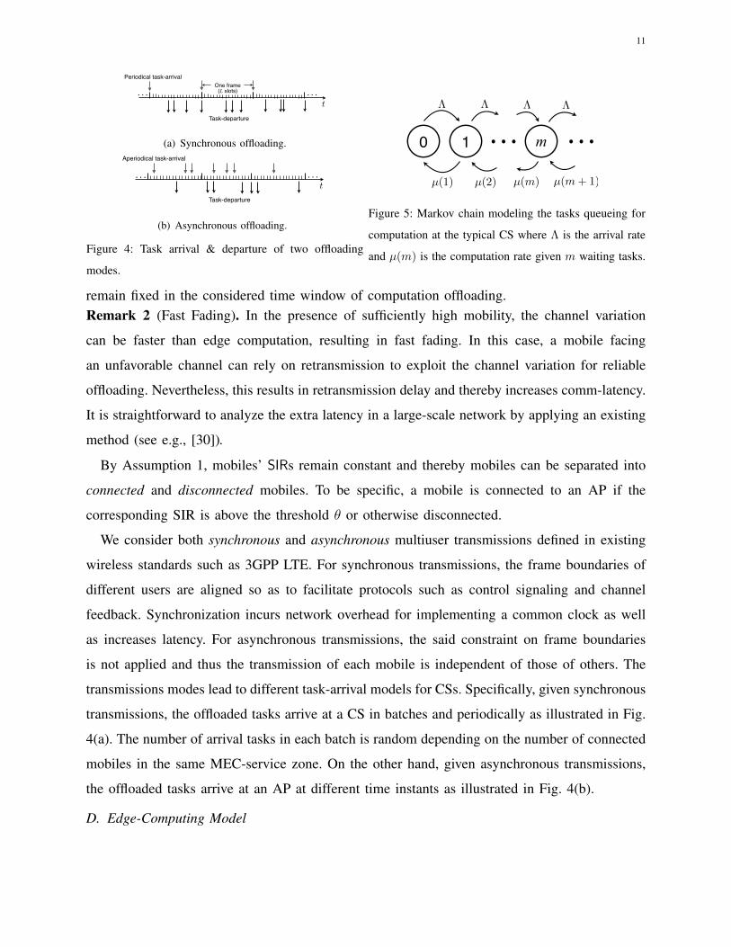
Figure 4: Task arrival & departure of two offloading

modes.

0 1 m

µ(1) µ(2) µ(m) µ(m + 1)

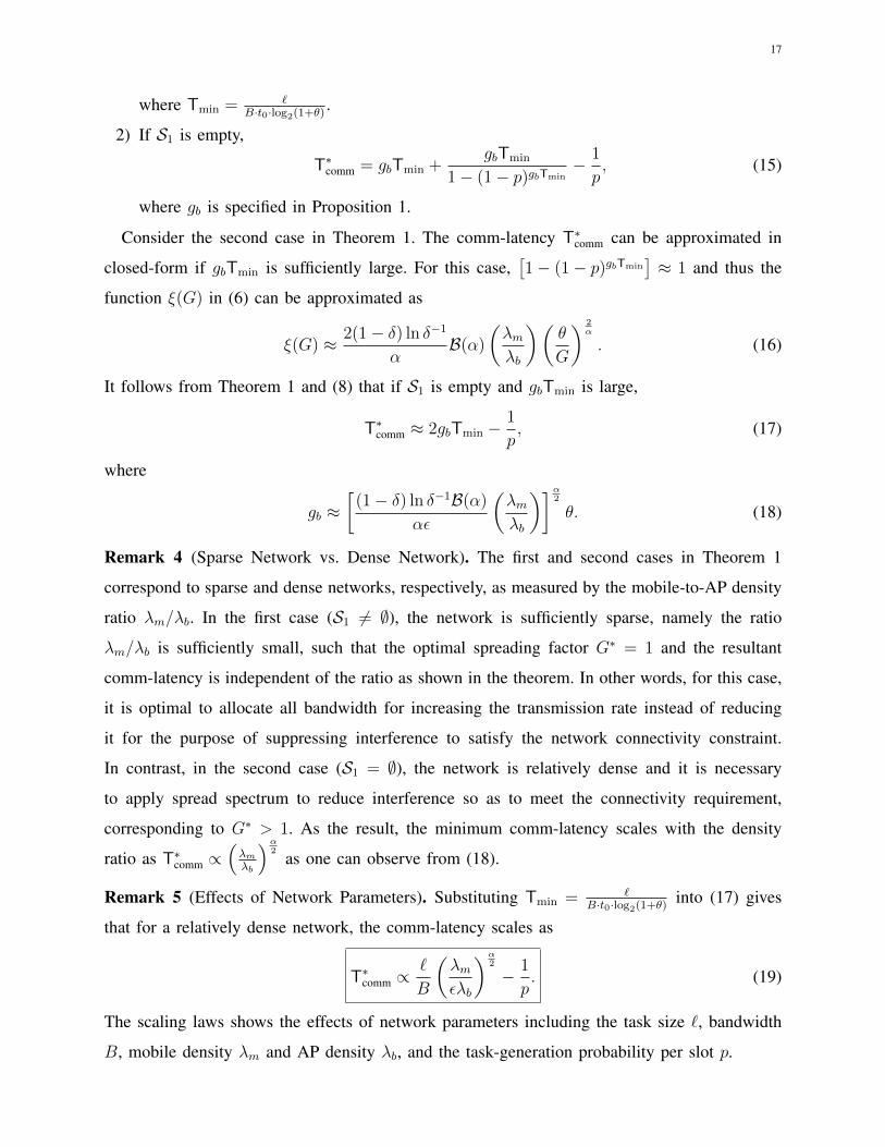
Figure 5: Markov chain modeling the tasks queueing for

computation at the typical CS where Λ is the arrival rate

and µ(m) is the computation rate given m waiting tasks.

remain fixed in the considered time window of computation offloading.Remark 2 (Fast Fading). In the presence of sufficiently high mobility, the channel variation

can be faster than edge computation, resulting in fast fading. In this case, a mobile facing

an unfavorable channel can rely on retransmission to exploit the channel variation for reliable

offloading. Nevertheless, this results in retransmission delay and thereby increases comm-latency.

It is straightforward to analyze the extra latency in a large-scale network by applying an existing

method (see e.g., [30]).

By Assumption 1, mobiles’ SIRs remain constant and thereby mobiles can be separated into

connected and disconnected mobiles. To be specific, a mobile is connected to an AP if the

corresponding SIR is above the threshold θ or otherwise disconnected.

We consider both synchronous and asynchronous multiuser transmissions defined in existing

wireless standards such as 3GPP LTE. For synchronous transmissions, the frame boundaries of

different users are aligned so as to facilitate protocols such as control signaling and channel

feedback. Synchronization incurs network overhead for implementing a common clock as well

as increases latency. For asynchronous transmissions, the said constraint on frame boundaries

is not applied and thus the transmission of each mobile is independent of those of others. The

transmissions modes lead to different task-arrival models for CSs. Specifically, given synchronous

transmissions, the offloaded tasks arrive at a CS in batches and periodically as illustrated in Fig.

4(a). The number of arrival tasks in each batch is random depending on the number of connected

mobiles in the same MEC-service zone. On the other hand, given asynchronous transmissions,

the offloaded tasks arrive at an AP at different time instants as illustrated in Fig. 4(b).

D. Edge-Computing Model

12

1) Parallel-Computing Model: Upon their arrivals at APs, tasks are assumed to be delivered

to CSs without any delay and queue at the CS buffer for computation on the first-come-first-

served basis. Moreover, each CS is assumed to be provisioned with large storage modelled as a

buffer with infinite capacity. At each CS, parallel computing of multiple tasks is implemented

by creating virtual machines (VM) on the same physical machine (PM) [35]. VMs are created

asynchronously such that a VM can be added or removed at any time instant. It is well known

in the literature that simultaneous VMs interfere with each other due to their sharing common

computation resources in the PM e.g., CPU, memory, buses for I/O. The effect is called I/O

interference that reduces the computation speeds of VMs. The model of I/O interference as

proposed in [35] is adopted where the expected computation time for a single task3, denoted by

Tc, is a function of the number of VMs, m:

Tc(m) = T0(1 + d)m−1, (3)

where T0 is the expected computation time of a task in the case of a single VM (m = 1) and

d is the degradation factor due to I/O interference between VMs. One can observe that Tc is a

monotone increasing function of d. For tractability, we assume that the computation time for a

task is an exp(Tc) RV following the common assumption in queueing theory [35].

2) CS Queuing Model: The general approach of analyzing comp-latency relies on the interplay

between parallel-computing and queueing theories. In particular, for the case of asynchronous

offloading, the task arrival at the typical AP is approximated as a Poisson process for the

following reasons. Due to the lack of synchronization between mobiles, the time instants of

tasks arrivals are approximately uniform in time. Furthermore, at different time instants, tasks

are generated following i.i.d. Bernoulli distributions based on the model in Section II-B. It is well

known that the superposition of independent arrival process behaves like a Poisson process [39].

Assumption 2. For the case of asynchronous offloading, given N connected mobiles and the

spreading factor G, the task arrivals at the typical AP are approximated as a Poisson process

with the arrival rate of Λ(N,G) = NpLL

= NpLGTmin

.

The Poisson approximation is shown by simulation to be accurate in Appendix III. Given the

Poisson arrival process and exponentially distributed computation time, the random number of

tasks queueing at the typical CS can be modelled as a continuous-time Markov chain as illustrated

in Fig. 5 [28]. In the Markov chain, Λ denotes the task-arrival rate in Assumption 2 and µ(k)3The latency caused by creating and releasing VMs is not explicitly considered. It is assumed to be part of computation time.

13

denotes the CS-computation rate (task/slot) given k tasks in the CS. The CS-computation rate

is maximized in the sequel by optimizing the number of VMs based on the queue length.

Last, the result-downloading phase is not considered for brevity. First, the corresponding

latency analysis is similar to that for the offloading phase. Second, the latency for downloading is

negligible compared with those for offloading. The reasons are that computation results typically

have small sizes compared with offloaded tasks and furthermore downlink transmission rates are

typically much higher than uplink rates.

E. Performance Metrics

The network performance is measured by two metrics: comm-latency and comp-latency. The

definitions of metrics build on the design constraints for ensuring network connectivity and

stability defined as follows.

Definition 1 (Network Coverage Constraint). The RAN in Fig. 2 is designed to be ε-connected,

namely that the portion of mobiles is no less than (1− ε), where 0 < ε 1.

The fraction of connected mobiles is equivalent to the success probability, a metric widely used

for studying the performance of random wireless networks [27]. For the MEC network, the

success probability is renamed as connectivity probability and defined for the typical mobile as

the following function of the spreading factor G:

pc(G) = Pr (SIR0 ≥ θ) , (4)

where SIR0 is given in (2). Then the network coverage constraint can be written as pc(G) ≥

(1− ε). Under the connectivity constraint, most mobiles are connected to APs. Then the comm-

latency, denoted as Tcomm, is defined as the expected duration required for a connected mobile

to offload a task to the connected AP successfully. The latency includes both waiting time at

the mobile’s buffer and and the transmission time.

Next, consider the computation load of the typical AP. Since the number of mobiles connected

to the AP is a RV, there exists non-zero probability that the AP is overloaded, resulting in infinite

queueing delay. In this case, the connected mobiles are referred to as being unstable. To ensure

most mobiles are stable, the following constraint is applied on the network design.

Definition 2 (Network Stability Constraint). The CSN in Fig. 2 is designed to be ρ-stable,

namely that the fraction of stable CSs is no less than (1− ρ), where 0 < ρ 1.

The fraction ρ is equivalent to the probability that the typical CS is stable, denoted as ps. Under

the stability constraint, most connected mobiles are stable. Then the comp-latency, denoted by

14

Tcomp, is defined for the typical connected mobile as the expected duration from the instant when

an offloaded task arrives at the serving CS until the instant when the computation of the task is

completed, which includes both queueing delay and actual computation time.

Last, given the above definitions, the network is referred to as being communication-limited

(comm-limited) if Tcomm Tcomp and computation-limited (comp-limited) if Tcomm Tcomp.

III. COMMUNICATION LATENCY ANALYSIS

In this section, the comm-latency defined in the preceding section is analyzed building on

results from the literature of network modeling using stochastic geometry. Then the latency is

minimized by optimizing the spreading factor for CDMA, which regulates the tradeoff between

the transmission rates of connected mobiles and network-connectivity performance.

A. Feasible Range of Spreading Factor

As mentioned, the spreading factor G is a key network parameter regulating the tradeoff be-

tween network coverage and comm-latency. To facilitate subsequent analysis, under the network

constraint in Definition 1, the feasible range of G is derived as follows. The result is useful

for minimizing the comm-latency in the next sub-section. To this end, consider the connectivity

probability defined in (4). Using a similar approach as the well-known one for deriving network

success probability using stochastic geometry (see e.g., [22]), we obtain the following result with

the proof omitted for brevity.

Lemma 1 (Connectivity Probability). Given the spreading factor G, the connectivity probability

of a typical mobile is given as

pc(G) =1− exp (−ξ(G))

ξ(G), (5)

where ξ(G) is defined as

ξ(G) =2(1− δ)

(1− (1− p)GTmin

)ln δ−1

αB(α)

(λmλb

)(θ

G

) 2α

, (6)

and B(α) ,∫ 1

0κ

2α−1(1− κ)−

2αdκ denotes the Beta function.

Recall that the network coverage constraint in Definition 1 requires that pc(G) ≥ (1 − ε).

Note that G is an important system parameter affecting both the transmission rates and the

connectivity probability as elaborated in the following remark.

Remark 3 (Transmission Rates vs. Connectivity). The spreading factor G of CDMA controls

the tradeoff between mobile transmission rates and network connectivity probability. On one

hand, increasing G reduces the bandwidth, BG

, available to each mobile, thereby reducing the

15

transmission rate and increasing comm-latency. As the result, given longer frames with the

task-generation rate being fixed, more mobiles are likely to have tasks for offloading at the

beginning of each frame, increasing the density of interferers. On the other hand, growing G

suppresses interference power by the factor G via spread spectrum. As a result, the connectivity

probability grows. Given the two opposite effects, one should expect that in the case of a stringent

connectivity constraint, either small or large value for G is preferred but no the moderate ones.

Next, the effects of the spreading factor as discussed in Remark 3 are quantified by deriving

the feasible range of G under the connectivity constraint. Define the Lambert function, W (x), as

the solution for the equation W (x)eW (x) = x. Then using the result in Lemma 1, the coverage

constraint pc(G) ≥ (1− ε) is equivalent to ξ(G) ≤ F(ε) with the function F(ε) defined as

F(ε) = W

(−e− 1

1−ε

1− ε

)+

1

1− ε. (7)

Notice that limε→0ddεW

(− e− 1

1−ε

1−ε

)= 1. Moreover, W

(− e− 1

1−ε

1−ε

)= −1 at ε = 0. It follows

that from these two results that F(ε) can be approximated as

F(ε) ≈ 2ε, ε 1. (8)

In addition, ξ(G) is maximized at the point of G = g0 of which the existence and uniqueness

are proved in Lemma 2. If ξ(g0) ≤ F(ε), it is straightforward that any G satisfies the condition

of (7). Otherwise, the feasible range of G satisfying the connectivity is provided in Proposition 1.

Lemma 2 (Properties of ξ(G)). The function ξ(G) in (6) attains its maximum at G = g0 with

g0 =αW

(− 2αe−

2α

)+ 2

αTmin ln(1− p). (9)

Moreover, ξ(G) is monotone increasing in the range [−∞, g0] and monotone decreasing in the

range [g0,∞].

Proof: See Appendix A.

Proposition 1 (Feasible Range of Spreading Factor). Under the network connectivity constraint,

the feasible range of G is G ≥ 1 if ξ(g0) ≤ F(ε), where g0 is given in (9). If ξ(g0) > F(ε), the

feasible range of G is S = S1

⋃S2 where

S1 = G ∈ Z+|1 ≤ G ≤ ga, S2 = G ∈ Z+|G ≥ gb, (10)

where ga and gb are the two roots of the equation ξ(G) = F(ε).

Based on Lemma 2, the function ξ(G) is monotone increasing over S1 but monotone decreasing

over S2. In addition, if ga < 1, S1 is empty and the feasibility range of G reduces to S2.

16

B. Communication Latency

Recall that the comm-latency of connected mobiles Tcomm comprises the expected waiting

time for offloaded tasks at mobiles, denoted as T(a)comm, and transmission delay, denoted as T

(b)comm.

Consider the expected waiting time. Recalling that the offloading protocol in Section II-B, the

first task arrival during L slots is delivered to the offloading buffer and the subsequent tasks

are forwarded to the local computation unit. Let K denote the slot index when an offloaded

task arrives at the offloading buffer. It follows that the probability distribution of K follows a

conditional geometric distribution, i.e., Pr(K = k) = p(1−p)k−1

1−(1−p)L , where k = 1, 2, · · · , L and the

normalization term 1−(1−p)L gives the probability that at least one task arrives during a single

frame. Thereby, the expected waiting time is given as

T(a)comm =

L∑k=1

(L− k)p(1− p)k−1

1− (1− p)L=

L

1− (1− p)L− 1

p. (11)

Next, consider the transmission time for a single task in a frame that spans L slots. Recall

that L = GTmin where Tmin is the minimum time for transmitting a task as defined earlier.

Combining T(b)comm = GTmin and T

(a)comm in (11) gives the following result.

Lemma 3 (Comm-Latency). Given the spreading factor G, the comm-latency of the typical

mobile Tcomm (in slot) is given as

Tcomm(G) = GTmin +GTmin

1− (1− p)GTmin− 1

p, (12)

where Tmin is the minimum time for transmitting a task using full bandwidth.

Next, consider the minimization of the comm-latency over the spreading factor G. Using

(12), it is straightforward to show that the comm-latency Tcomm(G) is a monotone increasing

function of G. Therefore, minimizing comm-latency is equivalent to minimizing G. It follows

from Proposition 1 that the minimum of G, G∗ = minG∈S

G, is given as

G∗ =

gb, S1 = ∅,

1, otherwise.(13)

Substituting G∗ into (12) gives the minimum comm-latency as shown in the following theorem.

Theorem 1 (Minimum Comm-Latency). By optimizing the spreading factor G, the minimum

comm-latency (in slot), denoted as T∗comm, is given as follows.

1) If S1 in (10) is non-empty,

T∗comm = Tmin +Tmin

1− (1− p)Tmin− 1

p, (14)

17

where Tmin = `B·t0·log2(1+θ)

.

2) If S1 is empty,

T∗comm = gbTmin +gbTmin

1− (1− p)gbTmin− 1

p, (15)

where gb is specified in Proposition 1.

Consider the second case in Theorem 1. The comm-latency T∗comm can be approximated in

closed-form if gbTmin is sufficiently large. For this case,[1− (1− p)gbTmin

]≈ 1 and thus the

function ξ(G) in (6) can be approximated as

ξ(G) ≈ 2(1− δ) ln δ−1

αB(α)

(λmλb

)(θ

G

) 2α

. (16)

It follows from Theorem 1 and (8) that if S1 is empty and gbTmin is large,

T∗comm ≈ 2gbTmin −1

p, (17)

where

gb ≈[

(1− δ) ln δ−1B(α)

αε

(λmλb

)]α2

θ. (18)

Remark 4 (Sparse Network vs. Dense Network). The first and second cases in Theorem 1

correspond to sparse and dense networks, respectively, as measured by the mobile-to-AP density

ratio λm/λb. In the first case (S1 6= ∅), the network is sufficiently sparse, namely the ratio

λm/λb is sufficiently small, such that the optimal spreading factor G∗ = 1 and the resultant

comm-latency is independent of the ratio as shown in the theorem. In other words, for this case,

it is optimal to allocate all bandwidth for increasing the transmission rate instead of reducing

it for the purpose of suppressing interference to satisfy the network connectivity constraint.

In contrast, in the second case (S1 = ∅), the network is relatively dense and it is necessary

to apply spread spectrum to reduce interference so as to meet the connectivity requirement,

corresponding to G∗ > 1. As the result, the minimum comm-latency scales with the density

ratio as T∗comm ∝(λmλb

)α2

as one can observe from (18).

Remark 5 (Effects of Network Parameters). Substituting Tmin = `B·t0·log2(1+θ)

into (17) gives

that for a relatively dense network, the comm-latency scales as

T∗comm ∝`

B

(λmελb

)α2

− 1

p. (19)

The scaling laws shows the effects of network parameters including the task size `, bandwidth

B, mobile density λm and AP density λb, and the task-generation probability per slot p.

18

C. Task-Arrival Rates at APs/CSs

The offloading throughput of the RAN represents the load of the CSN (see Fig. 2). The

throughput can be measured by the expected task-arrival rate (in number of tasks per slot) at the

typical AP (equivalently the typical CS). Its scaling law with the expected number of mobiles

per AP, λm/λb, is not straightforward due to several factors. To be specific, the total bandwidth

is fixed, the spread factor grows nonlinearly with λm/λb, and the likelihood of task-generation

probability per frame varies with the frame length. To address this issue, the task arrivals at the

typical AP are characterized as follows.

Consider the case of asynchronous offloading. Based on the model in Section II-B, the

probability that a mobile generates a task for offloading in each frame is

p∗L = 1− (1− p)L∗ , (20)

where L∗ is the frame length given the optimal spreading factor G∗ in (13). The expected task-

offloading rate (in number of tasks per slot) for the typical mobile, denoted as β∗, is given as

β∗ =p∗LL∗

. Since L∗ = G∗Tmin,

β∗ =1− (1− p)G∗Tmin

G∗Tmin

. (21)

where β∗ = p∗L · G∗Tmin. Let Λ∗ denote the expected task-arrival rate at the typical AP (or

CS). Then Λ∗ = Nβ∗ where N is the expected number of mobiles connected to the AP. Since

N = (1− δ)(1− ε)λmλb

,

Λ∗ = (1− δ)(1− ε)λmλbβ∗. (22)

Remark 6 (Effects of Network Parameters). Using (13), (18) and (21), one can infer that

Λ∗ ∝

pλmλb,

λmλb→ 0,

B

(λmλb

)−α2

+1

,λmλb→∞.

(23)

The first case corresponds to a sparse network whose performance is not limited by bandwidth

and interference. Then the expected task arrival-rate grows linearly with the task-generation

probability per slot, p, and the expected number of mobiles per AP, λm/λb. For the second

case, in a dense network that is bandwidth-and-interference limited, the rate grows linearly

the bandwidth B, but decreases with λm/λb. The reason for the decrease is the bandwidth for

offloading is reduced so that a larger spreading factor is available for suppressing interference

19

to meet the network-coverage requirement. Consequently, the load for the CSs is lighter for a

dense (thus comm-limited) network, reducing comp-latency as shown in the sequel.

Consider tasks arrivals for the case of synchronous offloading. Unlike the asynchronous

counterpart with arrivals spread over each frame, the tasks from mobiles arrive the typical AP

at the beginning of each frame. Thus, it is useful to characterize the expected number of task

arrivals per frame, denoted as A∗, which can be written as A∗ = Np∗L. It follows that

A∗ = (1− δ)(1− ε)λmλbp∗L. (24)

Remark 7 (Effects of Network Parameters). In a dense network (λm/λb →∞), it can be obtained

from (13), (18), and (20) that p∗L ≈ 1. Then it follows from (24) that the expected number of

tasks per frame increases linearly with the expected number of mobiles per AP, λm/λb.

IV. COMPUTATION LATENCY ANALYSIS: ASYNCHRONOUS OFFLOADING

This section aims at analyzing the comp-latency of the asynchronous offloading where task

arrival and departure are randomly distributed over time. Given the Markov model of Fig. 5, we

derive the network stability condition in Definition 2 and bounds of the average comp-latency.

A. Optimal Control of VMs

On one hand, creating a large number of VMs at the typical CS can slow down its computation

rate due to the mentioned I/O interference between VMs. On the other hand, too few VMs can

lead to marginal gain from parallel computing. Therefore, the number of VMs should be optimally

controlled based on the number of waiting tasks. To this end, let µ(m) denote the computation

rate given m VMs. Given the computation model in (3), it follows from µ(m) = m/Tc(m) that:

µ(m) =m

T0

(1 + d)1−m. (25)

By analyzing the derivative of µ(m), one can find that the function is monotone increasing

before reaching a global maximum and after that it is monotone decreasing. Thereby, the value

of m that maximizes µ(m), denoted as mmax, can be found with the integer constraint

mmax = round(

1

ln(1 + d)

), (26)

where round(x) rounds x to the nearest integer. The said properties of the function µ(m) and

the derived mmax in (26) suggest the following optimal VM-control policy.

Proposition 2 (Optimal VM Control). To maximize the computation rate at the typical CS, the

optimal VM-control policy is to create mmax VMs if there are a sufficient number of tasks for

20

computation or otherwise create as many VMs as possible until the buffer is empty. Consequently,

the maximum computation rate, denoted as µ∗(m), given m tasks at the CS (being computed or

in the buffer) is

µ∗(m) =

m

T0

(1 + d)1−m, 1 ≤ m ≤ mmax,

mmax

T0

(1 + d)1−mmax , m > mmax,(27)

where mmax is given in (26).

For ease notation, the maximum computation rate, µ(mmax), is re-denoted as µmax hereafter.

B. Computation Rates under Network Stability ConstraintThis subsection focuses on analzying the condition for the maximum computation rate of the

typical CS to meet the network stability constraint in Definition 2. The analysis combines the

results from queueing theory, stochastic geometry and parallel computing. The said constraint

requires ρ-fraction of mobiles, or equivalently ρ-fraction of CSs, to be stable, namely that comp-

latency is finite. According to queuing theory, stabilizing a typical CS requires that the task-arrival

rate Λ should be strictly smaller than the maximum departure rate µ∗(mmax): Λ < µmax [28].

Note that the former is a RV proportional to the random number of mobiles, N , connected to

the typical CS while the latter is a constant. Then the stability probability ps is given as

ps = Pr[Λ < µmax] = Pr

[N <

µmax

β∗

], (28)

where β∗ is the task-offloading rate given in (21). It follows from the network spatial model that

N is a Poisson distributed RV with the mean N = (1− δ)(1− ε)λmλb

. Using the distribution and

(28) and applying Chernoff bound, we can obtain an upper bound on the maximum computation

rate required to meet the stability constraint as shown below.

Proposition 3 (Computation Rates for ρ-Stability). For the CSN to be ρ-stable, a sufficient

condition for the maximum computation rate of the typical CS is given as

µmax ≥ Λ∗ · exp

(W

(− ln(ρ)

Ne− 1

e

)+ 1

), (29)

where W (·) is the Lambert function, the expected mobiles connected to the typical CS N =

(1− δ)(1− ε)λmλb

, and Λ∗ represents the expected arrival rate given in (22).

Proof: See Appendix B.

The above result shows that to satisfy the network-stability constraint, the maximum compu-

tation rate of each CS, µmax, should be larger than the expected task-arrival rate, Λ∗, scaled by

21

a factor larger than one, namely the exponential term in (29). Moreover, the factor grows as the

stability probability (1− ρ) increases.

Last, it is useful for subsequent analysis to derive the expected arrival rate conditioned on that

the typical CS is stable as shown below.

Lemma 4 (Expected Task-Arrival Rates for Stable CSs). Given that the typical CS is stable, the

expected task-arrival rate is given as

E[Λ|Λ < µmax] = Λ∗(

1− Pr(N = bRc)1− ρ

), (30)

where R = µmax

β∗measures the maximum number of mobiles the CS can serve, β∗ is the task-

offloading rate per mobile in (21), N and Λ∗ follow those in Proposition 3, and the Poisson

distribution function Pr(N = n) = Nne−N

n!.

Proof: See Appendix C.

C. Expected Computation Latency

In this subsection, the expected comp-latency, Tcomp, is analyzed using the Markov chain

in Fig. 5 and applying queueing theory. Exact analysis is intractable due to the fact that the

departure rate µ(m) in the Markov chain is a non-linear function of state m. This difficulty is

overcome by modifying the Markov chain to give two versions corresponding to a M/M/m and

a M/M/1 queues, yielding an upper and a lower bounds on Tcomp, respectively.

First, consider upper bounding Tcomp. To this end, the departure rate µ(m) in the Markov

chain in Fig. 5 with the following lower bound obtained by fixing all exponents as (1−mmax):

µ−(m) =

mT0

(1 + d)1−mmax , 1 ≤ m ≤ mmax,

mmax

T0(1 + d)1−mmax , m > mmax.

(31)

As a result, the modified Markov chain is a M/M/mmax queue. The corresponding waiting time,

denoted as T+comp, upper bounds Tcomp since it reduces the computation rate. Applying classic

results on M/M/m queues (see e.g., [28]), the waiting time, T+comp, for task arrival rate Λ is

T+comp(Λ) =

mmax

µ−(mmax)+

τ(

Λµ−(mmax)

)mmax

mmax!µ−(mmax)(

1− Λmmaxµ−(mmax)

)2 , (32)

where the coefficient τ is given as

τ =

[mmax−1∑m=0

1

m!

(Λ

µ−(mmax)

)m+

∞∑m=mmax

mmmax−mmax

mmax!

(Λ

µ−(mmax)

)m]−1

. (33)

Using (30), (31) and (32), the upper bound is given in the following theorem.

22

Theorem 2.A (Comp-Latency for Asynchronous Offloading). Consider asynchronous offloading.

The average comp-latency is upper bounded as

Tcomp ≤mmax

µmax

+

(mmax

µmax

)2

· Λ∗

(mmax − 1)! (mmax − 1)2 ·(

1− Pr(N = bRc)1− ρ

), (34)

where R follows that in Lemma 4, and Λ∗ and µmax are specified in (22) and (27), respectively.

Proof: See Appendix D.

Note that the positive factor(

1− Pr(N=bRc)1−ρ

)accounts for Poisson distribution of mobiles.

Next, a lower bound on Tcomp is obtained as follows. One can observe from the Markov chain

in Fig. 5 that for states m ≤ mmax, the departure rates are smaller than the maximum, µmax.

The reason is that for these states, there are not enough tasks for attaining the maximum rate

by parallel computing. Then replacing all departure rates in the said Markov chain with the

maximum µmax leads to a lower bound on Tcomp. The resultant Markov chain corresponds to a

M/M/1 queue. Then using the modified Markov chain and the well-known results from M/M/1

queue (see e.g., [28]), the comp-latency for given arrival rate Λ can be lower bounded as

Tcomp(Λ) ≥ 1

µmax − Λ. (35)

By taking expectation over Λ and applying Jensen’s inequality,

Tcomp = E[Tcomp(Λ)] ≥ E

[1

µmax − Λ

∣∣∣∣Λ < µmax

]≥ 1

µmax − E[Λ|Λ < µmax]. (36)

Using (36) and Lemma 4, we obtain the following result.

Theorem 2.B (Comp-Latency for Asynchronous Offloading). Consider asynchronous offloading.

The average comp-latency is lower bounded as

Tcomp ≥1

µmax − Λ∗ ·(

1− Pr(N=bRc)1−ρ

) , (37)

where R follows that in Lemma 4, and Λ∗ and µmax are specified in (22) and (27), respectively.

Remark 8 (Computation-Resource Provisioning). Consider a MEC network provisioned with

sufficient computation resources, µmax/Λ∗ 1. It follows from Theorem 2.B

Tcomp ≥1

µmax

(1 +

c1Λ∗

µmax

),

where c1 is a constant. This lower bound has a similar form as the upper bound in Theorem

2.A. From these results, one can infer that the comp-latency for asynchronous offloading can be

approximated written in the following form:

Tcomp ≈c2

µmax

(1 +

c3Λ∗

µmax

),

µmax

Λ∗ 1, (38)

23

where c2, c3 are constants. The result suggests that to contain comp-latency, the provisioning of

computation resources for the MEC network must consider two factors. First of all, the maximum

computation rate, µmax, for each CS must be sufficient large. At the same time, the computation

rate must scale linearly with the total arrival rate such that the computation resource allocated

for a single offloaded task, measured by the ratio µmax/Λ∗, is sufficiently large.

D. Energy EfficiencyBased on the above analytical results so far, the subsection tempts to discuss the energy

savings of offloading than local computing. First, the energy consumption of offloading, denoted

by Eoff , can be derived via multiplying mobile’s transmission power P by the offloading duration

G∗Tmin. To satisfy the minimum average signal strength at the boundary of the MEC service

zone, P should scale with the radius r0 as P ∝ rα0 . Recalling r0 ∝ λ− 1

2b and Tmin ∝ ` where `

is the task size, the resultant energy consumption of Eoff is given as

Eoff = c4G∗`

λbα2

, (39)

where c4 is a constant depending on the minimum signal strength and Tmin. Next, it is well

studied in [6] that the optimal Eloc is proportional to `3, and inversely proportional to the square

of the deadline requirement which could be set as the total latency Tcomm + Tcomp without loss

of generality. Thus, Eloc is given as

Eloc = c5`3

(Tcomm + Tcomp)2, (40)

where c5 is a constant depending on the chip architecture. where c5 is a constant depending on

the chip architecture. As a result, the condition of energy savings, namely Eoff < Eloc, is given

in terms of ` and λb as

`2λα2b >

c4

c5

G∗ (Tcomm + Tcomp)2 . (41)

It is observed that the right-side of (41) is dominantly affected by the expected number of mobilesλmλb

(see (17), (18), (23) and (38)). In other words, given a mobile density λm and the task size

`, there exists the minimum density of APs λb to satisfy the condition in (41). Then under the

condition in (41), the energy savings due to offloading is given as Eloc − Eoff with Eoff and Eloc

given in (39) and (40), respectively.

E. MEC Network Provisioning and Planning

Combining the results from the preceding analysis on comm-latency and comp-latency yields

some guidelines for the provisioning and planning of a MEC network as discussed below. Assume

24

that the network is required to support computing for mobiles with density λm with targeted

expected comm-latency Tcomm and comp-latency Tcomp. The network resources are quantified by

the bandwidth B, the density of AP (or CS) λb, the maximum computing rate of each CS µmax.

First, consider the planning of the RAN. Combining the above results suggest the following

guidelines for network provisioning and planning. As shown in Section III-C, under the network-

coverage constraint (1−ε), the expected task-arrival rate at a AP, representing the RAN offloading

throughput, is a quasi-concave function of the expected number of mobiles per AP, λm/λb, with

a global maximum. Therefore, given a mobile density λm, the AP density should be chosen

for maximizing the RAN offloading throughput. Next, based on results in Theorem 1 and (21),

sufficient large channel bandwidth B should be provisioned to achieve the targeted Tcomm for

given mobile and AP densities, mobile task-generation rates, and task sizes.

Next, consider the planning of the CSN. Under the network-stability constraint, the maximum

CS computing rate for parallel computing should be planned to be larger than the expected task-

arrival rate scaled by a factor larger than one, which is determined by the allowed fraction of

unstable CSs (see Proposition 3). Then, the maximum computing rate should be further planned

to achieve the targeted Tcomp for computing an offloaded task using Theorems 2.A and 2.B.

V. COMPUTATION LATENCY ANALYSIS: SYNCHRONOUS OFFLOADING

In the preceding section, the process of asynchronous task arrival at a CS can be approximated

using a Markov chain, allowing tractable analysis of comp-latency using theories of M/M/m

and M/M/1 queues. This approach is inapplicable for synchronous offloading and the resultant

periodic task arrivals at the CS. Though tractable analysis in general is difficult, it is possible

for two special cases defined as follows.

Definition 3 (Special Cases: Light-Traffic and Heavy-Traffic). A light-traffic case refers to one

that the task-arrival rate is much smaller than the computation rate such that the queue at the

CS is always empty as observed by a new arriving task. In contrast, a heavy-traffic case refers

to one that the task-arrival rate is close to the computation rate such that there are always at

least mmax tasks in the queue.

The comp-latency for these two special cases are analyzed to give insights into the performance

of CSN with underloaded CSs and those with overloaded CSs.

A. Expected Computation Latency with Light-Traffic

First, the dynamics of the task queue at the typical CS is modelled as follows. Recall that

task arrivals are periodical, occurring at the beginning of every frame. Consider the typical CS.

25

Let Qt and At denote be the numbers of existing and arriving tasks at the beginning of frame t,

respectively, and Ct the number of departing tasks during frame t. Then the evolution of Qt can

be described mathematically as

Qt+1 = max [Qt +At+1 − Ct, 0] . (42)

The general analysis of comp-latency using (42) is difficult. The main difficulty lies in deriving

the distribution of Ct that depends on the number of VMs that varies continuously in time since

the computation time for simultaneous tasks are random and inter-dependent. To overcome the

difficulty, consider the case of light-traffic where a number of offloaded tasks arrives at the

typical CS to see an empty queue and an idling server. Correspondingly, the evolution equation

in (42) is modified such that given At+1 6= 0, Qt = Ct = 0, yielding Qt+1 = At+1.

Next, given this simple equality, deriving the expected comp-latency reduces to analyzing the

latency for computing a random number of A tasks at the CS, which arrives at the beginning

of an arbitrary frame. Without loss of generality, the tasks are arranged in an ascending order

in terms of computation time and referred to as Task 1, 2, · · · ,A. Moreover, let Ln denote the

expected computing time for Task n and hence L1 ≤ L2 ≤ · · · ≤ LA. Then the expected

comp-latency Tcomp can be written in terms of Ln as

Tcomp = EA

[∑An=1 LnA

∣∣∣∣∣A > 0

]. (43)

To obtain bounds on Tcomp in closed form, a useful result is derived as follows. Given m

VMs, recall that the computation time of a task follows the exponential distribution with the

mean being the inverse of the computation rate µ(m) in (27). Using the memoryless property

of exponential distribution, a useful relation between Ln is obtained as

Ln = Ln−1 +1

µ(m)=

Ln−1 +

1

µmax

, 1 ≤ n ≤ A−mmax + 1,

Ln−1 +1

µ(A− n+ 1), otherwise,

(44)

with L0 = 0. Note that µ(1) ≤ µ(m) ≤ µmax for all m. Thus, it follows from (44) that

n

µmax

≤ Ln ≤n

µ(1). (45)

Substituting (45) into (43) gives

1

µmax

· EA

[∑An=1 n

A

∣∣∣∣∣A > 0

]≤ Tcomp ≤

1

µ(1)· EA

[∑An=1 n

A

∣∣∣∣∣A > 0

]. (46)

26

Recalling the number of arriving tasks A follows a Poisson RV with mean A∗ of (24), bounds

on the comp-latency is obtained shown in the following theorem.

Theorem 3 (Comp-Latency for Synchronous Offloading). Consider the case of synchronous

offloading with light-traffic. The expected comp-latency can be bounded as

1

2µmax

(1 +

A∗

1− e−A∗)≤ Tcomp ≤

1

2µ(1)

(1 +

A∗

1− e−A∗).

where A∗ is the expected number of arriving tasks to the typical CS per frame given in (24).

Remark 9 (Comparison with Asynchronous Offloading). From the results in the above theorem,

one can infer that for the current case, the comm-latency can be approximated as

Tcomp ≈

1

µ(1), A∗ → 0,

A∗

2µ(mmax), A∗ 1.

(47)

Comparing the expression with the counterpart for asynchronous offloading in (38), it is unclear

which case leads to longer comp-latency. However, simulation shows that in general, synchro-

nizing offloading tends to incur longer latency by overloading CSs and thereby suffering more

from I/O interference in parallel-computing.

B. Expected Computation Latency with Heavy-Traffic

This subsection focuses on analyzing the expected comp-latency, Tcomp, for the case of heavy-

traffic as defined in Definition 3. For this case, with the queue being always non-empty, the

equation in (42) describing the queue evolution reduces to Qt+1 = Qt +At − Ct. The key step

in deriving Tcomp is to apply the said equation to the analysis of the expected queue length. The

technique involves taking expectation of the squares of the two sides of the equation as follows:

E[Q2t+1

]= E

[(Qt +At − Ct)2] = E

[Q2t

]+ E

[(At − Ct)2]+ 2E [Qt(At − Ct)] . (48)

Since Qt, At and Ct are independent of each other and E[Q2t+1

]= E [Q2

t ] given the stable CS,

E [Q] =E [A2] + E [C2]− 2E [A]E [C]

2 (E [C]− E [A]), (49)

where the subscripts t of Qt, At and Ct are omitted to simplify notation. Given the number of

connected mobiles, N , the number of arrival tasks A follows a Poisson distribution with the first

and second moments being E (A | N) = Np∗L and E (A2 | N) = Np∗L + (Np∗L)2 respectively,

where the task-offloading probability p∗L is given in (20). Next, under the heavy-traffic assump-

tion, the total computation rate of the CS is µmax. It follows that the departure process at the

27

typical CS is Poisson distributed where the first and second moments are E[C] = µmaxL∗ and

E[C2] = µmaxL∗ + [µmaxL

∗]2, respectively. Substituting the results into (49) gives

E [Q | N ] =Np∗L

µmaxL∗ −Np∗L+

1

2· (µmaxL

∗ −Np∗L) +1

2. (50)

In addition, to satisfy the condition for stabilizing the CS, the arrival rate E [A] should be strictly

smaller than the departure rate E[C]. This places a constraint on the maximum of N , namely that

N ≤ bRc with R defined in Lemma 4. Under this constraint, applying Little’s theorem obtains

the expected comp-latency Tcomp as

Tcomp =

E

[E [Q | N ]

E [A | N ]

∣∣∣∣N ≤ bRc]− 1

2

· L∗. (51)

Combining (50) and (51) yields the main result of this sub-section as shown below.

Theorem 4 (Comp-Latency for Synchronous Offloading). Consider the case of synchronous

offloading with heavy-traffic. The expected comp-latency is given as

Tcomp =

1

p∗LE

[1

R−N

]+

1

2

(R +

1

p∗L

)E

[1

N

]− 1

L∗, (52)

where the constant R and the distribution of N follow those in Lemma 4.

Remark 10 (Comparison with Asynchronous Offloading). By applying Jensen’s inequality, the

comp-latency of (52) can be lower bounded as

Tcomp ≥1

µmax − c4Λ∗+L∗

2· µ(mmax)

c4Λ∗+

1

c4Λ∗− L∗, (53)

where c4 is a constant. Since for the case of heavy-traffic, the task-arrival rate c4Λ∗ approaches

the maximum computation rate µmax,

Tcomp ≥1

µmax − c4Λ∗, c4Λ∗ → µmax. (54)

The above lower bound has the same form as the asynchronous-offloading counterpart in (37).

Both diverge as the task-arrival rate approaches the maximum computation rate.

VI. SIMULATION RESULTS

In this section, analytical results on comm-latency and comp-latency are evaluated by simu-

lation. The simulation parameters have the following default settings unless specified otherwise.

The densities of APs and mobiles are λb = 2× 10−2 m−2 and λm = 5× 10−2 m−2, respectively.

The SIR threshold is set as θ = 1 dB and the path-loss exponent is α = 3. For the network

coverage parameter δ is δ = 10−2, corresponding to the radius of MEC service zone being

r0 = 12m. The total bandwidth is B = 6 MHz. The data size per task is fixed as ` = 0.5× 106

28

Mobile density (0.1/sq. m)0.4 0.6 0.8 1 1.2 1.4 1.6 1.8

Ave

rage

Lat

ency

(sec

)

0

0.2

0.4

0.6

0.8

1

1.2

1.4

1.6

1.8

2

Comp-Latency: Upper BoundComp-Latency: SimulationComp-Latency: Lower BoundComm-Latency: Simulation/AnalysisTotal Latencies: Simulation

Comp-limited Comm-limitedComm-limited

(a) Effect of mobile density.

Task Generation Rate (task/slot)0.1 0.2 0.3 0.4 0.5 0.6 0.7 0.8 0.9 1

Ave

rage

Lat

ency

(sec

)

0

0.2

0.4

0.6

0.8

1

1.2

1.4

1.6

1.8

2

Comp-Latency: Upper BoundComp-Latency: SimulationComp-Latency: Lower BoundComm-Latency: Simulation/AnalysisTotal Latencies: Simulation

Comm-limited Comp-limited

(b) Effect of task generating rate.Figure 6: Comparisons between comm-latency and comp-latency for the case of asynchronous offloading.

bits. The single-task computation time T0 in the parallel-computation model is set as T0 = 0.1

(sec) and the factor arising from I/O interference is d = 0.2. The task generation probability per

slot is p = 0.2. The parameters ε and ρ are both set as 0.05.

We present the comparisons between Monte Carlo simulations (104 realizations) and analytical

results in all figures. For each realization, both mobiles and APs are distributed in the plane

based on the PPPs. Each mobile randomly generates an offloading task and transmits it to its

corresponding AP. Then the AP generates VMs and performs the computation upon the task

arrivals. A queue of tasks will appear if the task arrival rate is large than the computation rate

(e.g., too many tasks arrived at the AP at the same time). The VM will be released when the

corresponding task is computed.

Fig. 6 compares expected comm-latency and comp-latency for the case of asynchronous

offloading. The effects of mobile density λm and task generating rate p are investigated and

several observations can be made. As shown in Fig. 6(a), the expected comp-latency as a function

of the mobile density is observed to exhibit the quasi-concavity described in Remark 4. In

contrast, the expected comm-latency is a monotone increasing function following the scaling law

in Remark 5. These properties lead to the partitioning of the range of mobile density into three

network-operation regimes as indicated in Fig. 6(a). In particular, the middle range corresponds to

comp-limited regime while others are comm-limited. Next, consider the effect of task-generation

rate at mobiles, specified by the task-generation probability p. Both types of latency are observed

to converge to corresponding limits as the rate grows. Their different scaling laws result in the

partitioning of the range of task-generation rate into comm-limited and comp-limited regimes.

Last, one can observe from both figures that the lower bound on comp-latency as derived in (37)

29

Mobile Density (0.1/sq. m)0.4 0.6 0.8 1 1.2 1.4 1.6 1.8

Ave

rage

Lat

ency

(sec

)

0

0.5

1

1.5

2

Comp-Latency: Heacy TrafficComp-Latency: SimulationComp-Latency: Upper Bound of Light TrafficComp-Latency: Lower Bound of Light TrafficComm-Latency: Simulation/AnalysisTotal Latencies: Simulation

Comm-limited

Comm-limitedComp-limited

(a) Effect of mobile density.

Task Generation Rate (task/slot)0.1 0.2 0.3 0.4 0.5 0.6 0.7 0.8 0.9 1

Ave

rage

Lat

ency

(sec

)

0.4

0.6

0.8

1

1.2

1.4

1.6

Comp-Latency: Heacy TrafficComp-Latency: SimulationComp-Latency: Upper Bound of Light TrafficComp-Latency: Lower Bound of Light TrafficComm-Latency: Simulation/AnalysisTotal Latencies: Simulation

Comm-limited Comp-limited

(b) Effect of task generating rate.Figure 7: Comparisons between comm-latency and comp-latency for the case of synchronous offloading.

is tighter than the upper bond therein.

Fig. 7 compares expected comm-latency and comp-latency for the case of synchronous offload-

ing. The same observations in the case of synchronous offloading also apply in the current case

except that the quasi-concavity of the expected comp-latency with respect to mobile density is

not shown in the considered range. Some new observations can be made as follows. Comparing

Fig. 6 and 7 shows that synchronizing offloading results in longer comp-latency. Next, the

center of the comp-limited range in Fig. 7(a) corresponds to the case of heavy-traffic studied

in Section V-B. Consequently, the derived upper bound on expected comp-latency for this case

is tight. For other ranges of mobile density, the bounds derived for the case of light traffic are

tighter. Last, Fig. 7(b) shows that the expected comp-latency is tightly approximated by bounds

derived for the light-traffic case when the task-arrival rate is small (≤ 0.3) and by that for the

heavy-traffic case when the rate is large (> 0.7), validating the results.VII. CONCLUSION REMARKS

In this work, we have first studied the network-constrained latency performance of a large-

scale MEC network, namely comm-latency and comp-latency under the constraints of RAN

connectivity and CSN stability. To study the tradeoffs between these metrics and constraints

and model the cascaded architecture of RAN and CSN, the MEC network has been modelled

using stochastic geometry featuring diversified aspects of wireless access and computing. Based

on the model, the average comm-latency and comp-latency have been analyzed by applying

the theories of stochastic geometry, queuing and parallel computing. In particular, their scaling

laws have been derived with respect to various network parameters ranging from the densities of

mobiles and APs to the computation capabilities of CSs. The results provide useful guidelines for

30

MEC-network provisioning and planning to avoid either the RAN or CSN being a performance

bottleneck.

The current work can be extended in several directions. In this work, we consider a single type

of computation task of which the task size and the average computation time are identical. How-

ever, considering different types of tasks makes the latency analysis more challenging but is of

practical relevance. Next, studying a large-scale hierarchical fog computing network comprising

mobiles, edge cloud and central cloud is aligned with recent advancements in edge computing.

Last, considering advanced techniques such as VM migration and cooperative computing to

reduce the latency will be another promising direction.APPENDIX

A. Proof of Lemma 2The first derivative of ξ(G) for G given in (6) can be derived as:

∂ξ(G)

∂G= −∆

α

(G−

2+αα

(αGTmin ln(1− p)(1− p)GTmin − 2(1− p)GTmin + 2

)), (55)

where ∆ = 2(1−δ) ln δ−1

αB(α)

(λmλb

)θ

2α . The existence of g0 is easily proved because (55) is strictly

positive and negative when G → 0 and G → ∞ respectively. Next, the solution of g0 to solve∂ξ(G)∂G

= 0 is g0 =αW

(− 2αe−

2α

)+2

αTmin ln(1−p) , where W (x) is the Lambert function. Since the value inside

the Lambert function is negative, there are two candidates for g0: one is from the principle

branch of Lambert function W(− 2αe−

2α

), and the other is the lower branch W−1

(− 2αe−

2α

).

The principle branch makes g0 = 0, but the lower branch satisfies g0 > 0, completing the proof.B. Proof of Proposition 3

Applying Chernoff bound on ps in (28) makes

ps ≥ 1− exp

(−µmax

β∗ln

(µmax

Nβ∗

)+µmax

β∗− N

)≥ 1− ρ, (56)

which is equivalent to µmax ≥ Λ∗ · exp(W(− ln(ρ)

Ne− 1

e

)+ 1)

as Proposition 3 shows.C. Proof of Lemma 4

Noting the expect task arrival of stable CSs is proportional to the average number of connected

mobiles. Therefore, we have E[Λ|Λ < µmax] = β∗ ·∑Rn=1 n·

Nne−Nn!

1−ρ = Nβ∗(

1− Pr(N=bRc)1−ρ

), where

Pr(N = bRc) = NbRce−N

bRc! , ending the proof.D. Proof of Theorem 2.A

Substituting τ = 1 into (32) and then applying(

Λµ−(mmax)

)mmax

≤ Λµ−(mmax)

as well as(1− Λ

mmaxµ−(mmax)

)2

≤(

1− 1mmax

)2

give an upper bound of T+comp(Λ) as

T+comp(Λ) ≤ mmax

µ−(mmax)+

Λµ−(mmax)

mmax!µ−(mmax)(

1− 1mmax

)2 . (57)

The spatial average on (57) based on Lemma 4 gives the final result in Theorem 2.A.

31

APPENDIX II: NOTATION TABLE

Notation Meaning

Ω, λb, Φ, λm PPP of APs, density of Ω, PPP of mobiles, density of Φ

r0, O(Y, r0), Offloading range, MEC service zone

L, p, pL Number of slots per frame, task-generating rate at mobile, task-offloading probability

η, g, α, θ, G Transmit power of AP, fading factor, path-loss exponent, SIR threshold, spreading factor

t0, B, `, d Slot length (in sec), Bandwidth per channel, number of bits per task, degradation factor of I/O interference

T0, Tcomm, Tcomp Expected computation time per task, average comm-latency, average comp-latency

Λ, µ, mmax, µmax Task arrival rate to CS, computation rate, maximal number of VMs, maximum computation rate

At, Ct, Qt Number of task arrival at frame t, number of task departure during frame t, the remaining tasks at frame t

ε, ρ, N Network coverage parameter, network stability parameter, expected number of mobiles connected to a AP

β∗, Λ∗, A∗ Expected task generation rate, expected task arrival rate, expected number of arrival tasks per frame

Table I: Summary of Notation

APPENDIX III: SUPPLEMENTARY SIMULATIONS

Mobile Density (0.1/sq. m)0.4 0.6 0.8 1 1.2 1.4 1.6 1.8

Ave

rage

Com

p-La

tenc

y (s

ec)

0.3

0.4

0.5

0.6

0.7

0.8

0.9

1

1.1

1.2

Sync: Poission Arrival Approx.Sync: SimulationAsync: Poission Arrival Approx.Async: Simulation

(a) Effect of mobile density.

Task Generation Rate (task/slot)0.1 0.2 0.3 0.4 0.5 0.6 0.7 0.8 0.9 1

Ave

rage

Com

p-La

tenc

y (s

ec)

0.2

0.3

0.4

0.5

0.6

0.7

0.8

0.9

1

Sync: Poission Arrival Approx.

Sync: Simulation

Async: Poission Arrival Approx.

Async: Simulation

(b) Effect of task generating rate.

Figure 8: Comparison to the Poisson Approximation in Assumption 2.

In Fig. 8, the the comp-latency of the Poisson arrival assumption of task-arrival process is

compared with that under the Poisson arrival assumption of Assumption 2, showing that the

tasks arrival process at AP can be well approximated to the Poisson task arrival assumption.

Fig. 9 represents the effects of AP density, which is shown that the same observations are

made in the case of decreasing mobile density.

Figs. 10 and 11 show the effects of the computation capability of CS, the computation time T0

and the degradation factor d, on the comp-latency for asynchronous and synchronous offloading

32

AP/CS Density (0.1/sq. m)0.05 0.1 0.15 0.2 0.25 0.3

Ave

rage

Lat

ency

(sec

)

0.2

0.4

0.6

0.8

1

1.2

1.4

1.6

1.8

2

Comp-Latency: Upper BoundComp-Latency: SimulationComp-Latency: Lower BoundComm-Latency: Simulation/AnalysisTotal Latencies: Simulation

(a) Asynchronous offloading.

AP/CS Density (0.1/sq. m)0.05 0.1 0.15 0.2 0.25 0.3

Ave

rage

Lat

ency

(sec

)

0

0.5

1

1.5

2

2.5

3Comp-Latency: Heacy TrafficComp-Latency: SimulationComp-Latency: Upper Bound of Light TrafficComp-Latency: Lower Bound of Light TrafficComm-Latency: Simulation/AnalysisTotal Latencies: Simulation

(b) Synchronous offloading.

Figure 9: Effects of AP (CS) density on comm-latency and comp-latency

Average computation time T0 (sec)0.05 0.06 0.07 0.08 0.09 0.1 0.11 0.12 0.13 0.14 0.15

Ave

rage

Com

p-La

tenc

y (s

ec)

0.2

0.4

0.6

0.8

1

1.2

1.4

Upper Bound

Simulation

Lower Bound

(a) Effect of edge-computing time per task.

Degradation Factor d0.1 0.15 0.2 0.25 0.3 0.35 0.4 0.45 0.5 0.55 0.6

Ave

rage

Com

p-La

tenc

y (s

ec)

0.4

0.6

0.8

1

1.2

1.4

1.6

1.8

2

Upper BoundSimulationLower Bound

(b) Effect of degradation factor due to I/O interference.

Figure 10: The performance of average latencies for the asynchronous offloading case.

cases, respectively. Both of the comp-latencies increase exponentially when the edge-computing

capability worse, i.e., T0 or d becomes larger, which agrees with the intuition.

Finally, we plot the ratio between the comp-latency of asynchronous and synchronous of-

floading cases in Fig. 12, which are always less than one because the comp-latency of the

asynchronous offloading is always smaller than the synchronous counterpart. Specifically, in

Fig. 12(a), the ratio first stays constant when mobiles is sparse and then decreases with mobile

density grows. As mobiles becomes denser, the number of offloading tasks at the beginning of

each frame increases, resulting in severe I/O interference than the asynchronous counterpart of

which the task arrivals are distributed over frame. On the other hand, in Fig. 12(b), it is observed

33

Average computation time T0 (sec)0.05 0.06 0.07 0.08 0.09 0.1 0.11 0.12 0.13 0.14 0.15

Ave

rage

-Com

p-La

tenc

y (s

ec)

0.3

0.4

0.5

0.6

0.7

0.8

0.9

1

1.1

1.2

1.3

Analysis: Heacy TrafficSimulationAnalysis: Upper Bound of Light TrafficAnalysis: Lower Bound of Light Traffic

(a) Effect of edge-computing time per task.

Degradation Factor d0.1 0.15 0.2 0.25 0.3 0.35 0.4 0.45 0.5 0.55 0.6

Ave

rage

Com

p-La

tenc

y (s

ec)

0.6

0.8

1

1.2

1.4

1.6

1.8

Analysis: Heacy TrafficSimulationAnalysis: Upper Bound of Light TrafficAnalysis: Lower Bound of Light Traffic

(b) Effect of degradation factor due to I/O interference.

Figure 11: The performance of average latencies for the synchronous offloading case. Both the light- and heavy-

traffic cases are plotted.

Mobile Density (0.1/sq. m)0.4 0.6 0.8 1 1.2 1.4 1.6 1.8 2

Com

p-La

tenc

y R

atio

: Asy

n/Sy

nc

0.5

0.55

0.6

0.65

0.7

0.75

0.8

0.85

0.9

0.95

1

(a) Effect of mobile density.

Task Generation Rate (task/slot)0.1 0.2 0.3 0.4 0.5 0.6 0.7 0.8 0.9 1

Com

p-La

tenc

y R

atio

: Asy

nc/S

ync

0.45

0.5

0.55

0.6

0.65

0.7

0.75

0.8

0.85

0.9

0.95

(b) Effect of task generation rate

Figure 12: The average comp-latency ratio: asynchronous offloading over synchronous offloading.

that the ratio grows and then converges to a constant when p increases. In other words, the gap of

comp-latency between two offloading cases is becoming smaller when the task arrival becomes

heaver, aligning with the discussion in Remark 10.

REFERENCES

[1] F. ETSI, Sophia Antipolis, “Mobile-edge computing introductory technical white paper,” Mobile-Edge Comput. Ind.

Initiative, White Paper, Sep. 2014.

[2] T. Taleb, K. Samdanis, B. Mada, H. Flinck, S. Dutta, and D. Sabella, “On multi-access edge computing: A survey of

the emerging 5G network edge architecture & orchestration,” IEEE Commun. Surveys Tuts., vol. 19, pp. 1657–1681, May

2017.

34

[3] Y. Mao, C. You, J. Zhang, K. Huang, and K. B. Letaief, “A survey on mobile edge computing: The communication

perspective,” IEEE Commun. Surveys Tuts., vol. 19, pp. 2322–2358, Fourthquarter 2017.

[4] N. Abbas, Y. Zhang, A. Taherkordi, and T. Skeie, “Mobile edge computing: A survey,” to appear in IEEE Internet Things

J.

[5] P. Mach and Z. Becvar, “Mobile edge computing: A survey on architecture and computation offloading,” IEEE

Communications Surveys Tuts., vol. 19, no. 3, pp. 1628–1656, 2017.

[6] W. Zhang, Y. Wen, K. Guan, D. Kilper, H. Luo, and D. O. Wu, “Energy-optimal mobile cloud computing under stochastic

wireless channel,” IEEE Trans. Wireless Commun., vol. 12, pp. 4569–4581, Sep. 2013.

[7] J. Kwak, Y. Kim, J. Lee, and S. Chong, “DREAM: Dynamic resource and task allocation for energy minimization in

mobile cloud systems,” IEEE J. Sel. Areas Commun., vol. 33, pp. 2510–2523, Dec. 2015.

[8] Y. Mao, J. Zhang, and K. Letaief, “Dynamic computation offloading for mobile-edge computing with energy harvesting

devices,” IEEE J. Sel. Areas Commun., vol. 34, pp. 3590–3605, Dec. 2016.

[9] C. You, K. Huang, and H. Chae, “Energy efficient mobile cloud computing powered by wireless energy transfer,” IEEE

J. Sel. Areas Commun., vol. 34, pp. 1757–1771, Mar. 2016.

[10] Y. Kao, B. Krishnamachari, M. Ra, and F. Bai, “Hermes: Latency optimal task assignment for resource-constrained mobile

computing,” IEEE Trans. Mobile Comput., vol. 16, pp. 3056–3069, Nov. 2017.

[11] J. Liu, Y. Mao, J. Zhang, and K. Letaief, “Delay-optimal computation task scheduling for mobile-edge computing systems,”

in Proc. of IEEE Int. Symp. Inf. Theory, pp. 1451–1455, Jul. 2016.

[12] S. Mahmoodi, R. Uma, and K. Subbalakshmi, “Optimal joint scheduling and cloud offloading for mobile applications,” to

appear in IEEE Trans. Cloud Comput.

[13] S.-W. Ko, K. Huang, S.-L. Kim, and H. Chae, “Live prefetching for mobile computation offloading,” IEEE Trans. Wireless

Commun., vol. 16, pp. 3057–3071, May 2017.

[14] C. You, K. Huang, H. Chae, and B. Kim, “Energy-efficient resource allocation for mobile-edge computation offloading,”

IEEE Trans. Wireless Commun., vol. 16, pp. 1397–1411, Mar. 2016.

[15] S. Sardellitti, G. Scutari, and S. Barbarossa, “Joint optimization of radio and computational resources for multicell mobile-

edge computing,” IEEE Trans. Signal Inf. Process. Netw., vol. 1, pp. 89–103, Jun. 2015.

[16] X. Chen, L. Jiao, W. Li, and X. Fu, “Efficient multi-user computation offloading for mobile-edge cloud computing,”

IEEE/ACM Trans. Networking, vol. 24, pp. 2795–2808, Oct. 2016.

[17] R. Kaewpuang, D. Niyato, P. Wang, and E. Hossain, “A framework for cooperative resource management in mobile cloud

computing,” IEEE J. Sel. Areas Commun., vol. 31, pp. 2685–2700, Dec. 2013.

[18] B. Rimal, D. Van, and M. Maier, “Mobile-edge computing vs. centralized cloud computing in fiber-wireless access

networks,” in Proc. of IEEE INFOCOM Workshop, pp. 991–996, 2016.

[19] T. Taleb, A. Ksentini, and P. Frangoudis, “Follow-me cloud: When cloud services follow mobile users,” to appear in IEEE

Trans. Cloud Comput.

[20] I. Farris, T. Taleb, H. Flinck, and A. Iera, “Providing ultra-short latency to user-centric 5G applications at the mobile

network edge,” Trans. Emerging Telecomm. Techn., Mar. 2017.

[21] H. ElSawy, E. Hossain, and M. Haenggi, “Stochastic geometry for modeling, analysis, and design of multi-tier and cognitive

cellular wireless networks: A survey,” IEEE Commun. Surveys Tuts., vol. 15, pp. 996–1019, Jan. 2013.

[22] J. G. Andrews, F. Baccelli, and R. K. Ganti, “A tractable approach to coverage and rate in cellular networks,” IEEE Trans.

Commun., vol. 59, pp. 3122–3134, Nov. 2011.

[23] H. Dhillon, R. Ganti, F. Baccelli, and J. Andrews, “Modeling and analysis of k-tier downlink heterogeneous cellular

networks,” IEEE J. Sel. Areas Commun., vol. 30, pp. 550–560, Mar. 2012.

35

[24] A. Sakr and E. Hossain, “Cognitive and energy harvesting-based D2D communication in cellular networks: Stochastic

geometry modeling and analysis,” IEEE Trans. Commun., vol. 63, pp. 1867–1880, Mar. 2015.

[25] R. Vaze and R. W. Heath, “Transmission capacity of ad-hoc networks with multiple antennas using transmit stream

adaptation and interference cancellation,” IEEE Trans. Inf. Theory, vol. 58, pp. 780–792, Feb. 2012.

[26] Y. Lin and W. Yu, “Downlink spectral efficiency of distributed antenna systems under a stochastic model,” IEEE Trans.

Wireless Commun., vol. 13, pp. 6891–6902, Dec. 2014.

[27] M. Haenggi, J. Andrews, F. Baccelli, O. Dousse, and M. Franceschetti, “Stochastic geometry and random graphs for the

analysis and design of wireless networks,” IEEE J. Sel. Areas Commun., vol. 27, pp. 1029–1046, Jul. 2009.

[28] D. Bertsekas and R. Gallager, Data networks. Prentice Hall, 1992.

[29] S. Barbarossa, S. Sardellitti, and P. Di Lorenzo, “Communicating while computing: Distributed mobile cloud computing

over 5g heterogeneous networks,” IEEE Signal Proc. Mag., vol. 31, pp. 45–55, Nov. 2014.

[30] M. Haenggi, “The local delay in poisson networks,” IEEE Trans. Inf. Theory, vol. 59, pp. 1788–1802, Mar. 2013.

[31] Z. Gong and M. Haenggi, “The local delay in mobile poisson networks,” IEEE Trans. Wireless Commun., vol. 12, pp. 4766–

4777, Sep. 2013.

[32] Y. Zhong, M. Haenggi, T. Quek, and W. Zhang, “On the stability of static poisson networks under random access,” IEEE

Trans. Wireless Commun., vol. 64, pp. 2985–2998, Jul. 2016.

[33] S. Verdu and S. Shamai, “Spectral efficiency of cdma with random spreading,” IEEE Trans. Inf. Theory, vol. 45, pp. 622–

640, Mar. 1999.

[34] L. Dai, B. Wang, Y. Yuan, S. Han, C.-L. I, and Z. Wang, “Non-orthogonal multiple access for 5g: solutions, challenges,

opportunities, and future research trends,” IEEE Commun. Mag., vol. 53, pp. 74–81, Sep. 2015.

[35] D. Bruneo, “A stochastic model to investigate data center performance and qos in iaas cloud computing systems,” IEEE

Trans. Parallel Distrib. Syst., vol. 25, pp. 560–569, Mar. 2014.

[36] J. He, Y. Wen, J. Huang, and D. Wu, “On the cost-qoe tradeoff for cloud-based video streaming under amazon ec2’s

pricing models,” IEEE Trans. Trans. Circuits Syst. deo Technol., vol. 24, pp. 669–680, Apr. 2014.

[37] B. Chang, L. Dai, Y. Cui, and Y. Xue, “On feasibility of p2p on-demand streaming via empirical vod user behavior

analysis,” in In Proc. Int. Conf. Distrib. Comput. Syst. Workshops, pp. 7–11, 2008.

[38] Y. Zhong, M. Haenggi, F.-C. Zheng, W. Zhang, T. Q. Quek, and W. Nie, “Towards a tractable delay analysis in large

wireless networks,” arXiv preprint arXiv:1612.01276.

[39] K. Sriram and W. Whitt, “Characterizing superposition arrival processes in packet multiplexers for voice and data,” IEEE

J. Sel. Areas Commun., vol. 4, pp. 833–846, Sep. 1986.