wireless communications dr. ranjan bose …...1 wireless communications dr. ranjan bose department...
TRANSCRIPT

1
Wireless Communications
Dr. Ranjan Bose
Department of Electrical Engineering
Indian Institute of Technology, Delhi
Lecture No. # 18
Mobile Radio Propagation - II (Continued)
Welcome to the next lecture on mobile radio propagation. Today we will talk about certain
channel parameters. Let us first look at the outline of today‟s talk.
(Refer Slide Time: 00:01:28 min)
We will summarize what we learnt last time. Then we will proceed with certain time dispersion
parameters which are mean excess delay, RMS or the root mean square delays spread and the
maximum excess delay over X dB. We will then learn about coherence bandwidth which is an
important channel characteristic. It is also useful for fading counter measure. We will look at
coherence time and how to determine coherence time for standard channels.

2
(Refer Slide Time: 00:02:08 min)
First let us start with a brief recap of our last lecture. We dealt with small scale multipath
measurement. We then discussed about various channel sounding techniques which were direct
RF pulse systems: spread spectrum sliding correlator channels sounding technique and frequency
domain channel sounding. We took the example of ultra-wideband or UWB measurement and
we first talked about the existing channel models for UWB. Then we discussed certain channel
measurement campaigns that have already been carried out by different companies and
universities. We talked about time domain and frequency domain measurements. We found the
equivalence of the two techniques: the time domain and the frequency domain measurements.
Finally, we discussed the Intel channel measurement campaign as well as the channel
measurement campaign for ultra-wideband carried out at IIT Delhi. today we will learn that a lot
of information obtained by doing channel measurements can help us determine channel
parameters which will in turn help us design better wireless systems. So what are the parameters
of a mobile multipath channel and how are they derived?
3
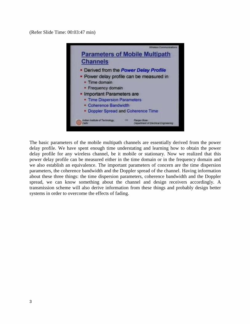
(Refer Slide Time: 00:03:47 min)
The basic parameters of the mobile multipath channels are essentially derived from the power
delay profile. We have spent enough time understating and learning how to obtain the power
delay profile for any wireless channel, be it mobile or stationary. Now we realized that this
power delay profile can be measured either in the time domain or in the frequency domain and
we also establish an equivalence. The important parameters of concern are the time dispersion
parameters, the coherence bandwidth and the Doppler spread of the channel. Having information
about these three things: the time dispersion parameters, coherence bandwidth and the Doppler
spread, we can know something about the channel and design receivers accordingly. A
transmission scheme will also derive information from these things and probably design better
systems in order to overcome the effects of fading.

4
(Refer Slide Time: 00:05:05 min)
Now a brief look at what the power delay profile is for small scale fading. The power delay
profile of the channel is simply found by taking the spatial average | hb(t,tau) |2 over a local area.
How small this local area depends whether it‟s an outdoor measurement campaign or indoor
measurement campaign, it can go from 2 m indoors to 6 m outdoors. if p(t) which is the pulse
being used to sound the channel has a time duration much smaller than the impulse response of
the multipath channel, in that case the received power delay profile in a local area is given by
P(tau), approximately equal to average value of k absolute value | hb(t; tau) |2, k is the scaling
factor. The „bar‟ represents the average over a local area and over several snapshots of hb(t; tau).
The gain k relates the transmitter power in the probing pulse p(t) to the total received power in a
multipath delay profile. Essentially it is a scale parameter. What we measured in most of the
cases is this. P(tau) is the averaged value that we measure in the oscilloscope.

5
(Refer Slide Time: 00:06:48 min)
So the measurements can be carried out by various channel sounding techniques. Plots of relative
received power as a function of excess delay with respect to a fixed time delay reference can be
taken out. The power delay profile is found by averaging instantaneous power delay
measurements over a local area. Now typically researchers use lambda/4, the quarter wavelength
for sampling interval. This is a rule of thumb. What do we mean by a local area? How big is a
local area? Well, it is less than 6 m outdoors. Suppose I am trying to do channel sounding for
GSM scenario or a WCDMA scenario, then I will go outdoors but my power delay profile would
be limited to about 6 m. the samples will be taken at approximately lambda/4. However, if I am
doing indoor channel measurement, then the power delay profile will be taken over 2 m only.
Again it is at quarter wavelength sampling intervals. Beyond that we come into the long term
fading. Not the small scale fading.

6
(Refer Slide Time: 00:08:20 min)
Let us look at one example of a typical measured power delay profile. Here in this figure, we
have on one axis, the delay in nanoseconds. So as you can see, it goes from0, 100,200 up to 600
ns of delay if the delay depends on your environment. On the other axis, we have the
measurement time in second. It shows that the channel now will be different from after 10 s or
100 s and so on and so forth. So the channel is varying with time. We will try to capture both the
inherent nature of the channel and the time varying nature of the channel by a different
measurements of coherence time and coherence bandwidth. On the z axis, we have put the signal
strength in dBm. So if you look at it carefully, if you just go along this axis, then for a particular
instant in time, we are taking the channel impulse response measurements and what we are
developing here is a notion of the reflections at close by locations given by this sharp peak here
and some for the reflections here and here. If we conduct the same experiment after say,100 or
200 s, we come up to here. So the channel has changed the reflectors have moved question.
Conversation between Student and Professor: The question being asked is: regarding the floor of
the received power, it appears from the figure that close to -80 dBm is what my floor is. What is
this figure -80 dBm? Does it relate to the noise floor? The answer is: yes. This apparently
represents the noise floor .the average received power obtained between the transmitter-receiver
separation kept at certain distance. You keep on receiving about -80 dB when you know
significant signal is received. The other strong reflected or line of sight components can be
obtained which are close to -50 dB or -70 dB or 60 dB. This also represents something as the
receiver sensitivity that we are dealing with. If my receiver was more sensitive, I can probably
get more signals below here also so that this is kind of a threshold level.

7
(Refer Slide Time: 00:11:16 min)
Let us look at another example. This time for the outdoor power delay profile, here is an example
of outdoor power delay measurements for a 900 MHz cellular system. on the x axis, there is the
excess delay in ms. please note when you carryout power delay measurements outside the excess
delay is of the order of ms whereas inside the room or indoor situations you are more likely to
find excess delay in ns. On the y axis, we have put the signal strength in dBm. Clearly there is a
line which is the threshold about the receiver sensitivity. So you can see that the power delay
profile varies a lot and you can see clearly that there are some clear reflections.
(Refer Slide Time: 00:12:24 min)

8
Now, on the other hand if you want to consider an indoor power delay profile measurement,
again on the x axis if you put the excess delay, please note this time you are working in the
domain of nanoseconds whereas on the y axis, you have the normalized received power. You see
for many stronger reflections spaced close by. If you go back, you will realize that the reflections
were far apart and there were some strong reflections and some weak reflections. Beyond a
certain time, you do not have much reflection. They go down drastically. This is an example for
a 4 GHz system. Later in today‟s talk, we will list out certain measurement data obtained for this
excess delay both in indoor as well as outdoor environments. It is interesting to note that this
excess delay is also a function of the frequency of operation. You will get a completely different
profile if you go from 4 GHz here to say 10 GHz or even to 900 MHz.
(Refer Slide Time: 00:13:39 min)
Let us now talk about the time dispersion parameters. The time dispersion parameters grossly
quantify the multipath channel. These parameters include first the mean excess delay, the root
mean square or RMS delay spread and of course the maximum excess delay. We will talk about
the X dB in a minute.

9
(Refer Slide Time: 00:14:11 min)
now the mean excess delay tau bar is the first moment of the power delay profile. So it is almost
like the first moment given by the power delay profile measured by an oscilloscope
mathematically tau bar = summation over k ak 2 tau k / by summation ak
2. Now ak represents the
path gain for the k th
path. If you are actually carrying out the power delay profile measurement,
then it is nothing but the power P (tau k). So if you are actually working from the power delay
profile curves, then you would not have to be bothered with ak. You don‟t have to square it. You
directly get the ak 2 / by summation over k P(tau k).
Conversation between student and professor: the question being asked is: what is meant by a
„subscript k‟ here is we are dealing with a multipath channel. So there is more than one path
from the transmitter to the receiver through reflections, scattering, diffraction, etc. for any
particular path, the signal gets path gain which is ak. It can be smaller than one. So if it is 0.1, it
means that for that particular path which I receive through reflections, the receiver strength is 0.1
times what I sent. Whereas for second path, the path gain might be different. What I could get is
a much stronger reflection. It‟s a better reflecting material. Maybe it‟s metal and the path gain for
that reflection will be larger. Line of sight will probably have the strongest a k. if there are 10
multipaths, and then k will start from 0 to 9. There will be 10 multipath components. Tau k
represents the delay associated with that path. If the reflector is located far away, then tau k will
be large. If the reflector is close by, tau k will be small. Soon we will look at an example to learn
how to calculate this mean excess delay. Please remember this term „mean excess delay‟ will
have some correlation with my maximum data rate that I can support in the channel. So these
measurements are important in designing our exact communication system.
10
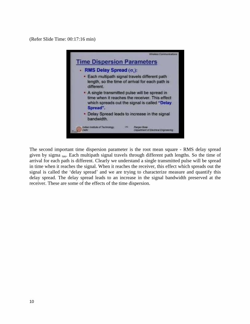
(Refer Slide Time: 00:17:16 min)
The second important time dispersion parameter is the root mean square - RMS delay spread
given by sigma tau. Each multipath signal travels through different path lengths. So the time of
arrival for each path is different. Clearly we understand a single transmitted pulse will be spread
in time when it reaches the signal. When it reaches the receiver, this effect which spreads out the
signal is called the „delay spread‟ and we are trying to characterize measure and quantify this
delay spread. The delay spread leads to an increase in the signal bandwidth preserved at the
receiver. These are some of the effects of the time dispersion.

11
(Refer Slide Time: 00:18:02 min)
How do we quantify this sigma tau? What is the physical interpretation of the RMS delay spread?
The RMS delay spread actually characterizes the time dispersiveness of the channel. So it is
obtained directly from the power delay profile. It indicates the delay during which the power of
the received signal is above a certain value. It is the square root of second central moment of the
power delay profile. Mathematically sigma tau is given by under root tau2 bar, the average value
of tau 2 – (tau bar)
2which is nothing but the second central moment of the power delay profile.
How do we obtain tau 2 average? It is given by summation over k multipath channels a k
2 tau k
2
where a k is the path gain of the kth
channel and tau k represents the delay associated with the kth
channel. Normalized by summation over k a k 2. If you are working with a digital oscilloscope
which averages, we directly get the power delay profile and we don‟t have to worry about the ak 2 we can directly plug in the values of P (tau k). First you calculate tau
2 bar; the average value
and then from that you obtain the sigma t which is nothing but the root mean square delay spread.

12
(Refer Slide Time: 00:20:02 min)
Here we have a table of the measured values of the actual RMS delay spread taking indoors and
outdoors by various researchers. if you see the left most column talks about the environment
where it is urban suburban and indoors there is a whole range of frequency that has been
deployed starting from close to 900 and 10 MHz up to 1900 MHz. now the RMS delay spread
that we were talking about by measurement is found out to be sigma t ranging from 1300 ns
average to 600 ns standard deviation and 35 ns maximum. You know dense urban city like
Newyork, indoors it is interesting to note that if you look at indoor office building and carry out
the same measurement either at 1500 MHz or 850 MHz, the root mean squared delay spread
changes. You have much smaller root mean square delay when you work at 1500 MHz whereas
if you go at 850 MHz much larger wavelength your maximum root mean square delay also
increases. So that is an interesting effect.

13
(Refer Slide Time: 00:21:34 min)
Let‟s talk about the time dispersion parameter maximum excess delay of X dB. It is the time
delay during which the multipath energy falls to X dB below the maximum. I am talking about
the strongest signal received; I take a line which is 10 dB if my X is 10 below my maximum
received power. In generally it is X dB below the maximum and then find out how many
reflections are there within that region. How many strong reflections are obtained till the
multipath energy falls to X dB below the maximum received power? So the maximum excess
delay is nothing but tau (X) - tau 0. Tau 0 represents the first marker for the received signal. Tau 0
is the first arriving signal. Tau x is the maximum delay at which a multipath component is within
X dB of the strongest arriving multipath signal. Please note that the strongest arriving multipath
signal necessarily doesn‟t mean it is the first one you get. You can have a much stronger reflector
and no line of sight in which case may be the second or the third reflected signal is the
maximum. I compare it with the maximum value. Not the first arriving value. So this maximum
excess delay defines the temporal extent of the multipath that is above a particular threshold.
Tau(x) is called the excess delay spread of a power delay profile.

14
(Refer Slide Time: 00:23:40 min)
Now let‟s look at an example from measured data. We have here on the x axis the excess delay
in nanoseconds. Clearly these measurement data have been taken in an indoor setting. On the y
axis ordinate, we have the normalized received power in dB. What we see is the signal as a large
enough delay spread but we would need to characterize it. So the first thing that we need to do is
to find out what is the mean excess delay which is the tau bar. So here from this measured data,
we can calculate for this particular sample. The mean excess delay comes out to be about 45 ns.
It is nothing but the statistical mean. But that is not the only thing we are interested in. we are
interested in also the maximum excess delay. Let‟s fix our threshold at 10 dB. So if 10 dB is our
threshold, then 10 dB is below the largest peak here. Luckily the first peak is the largest.
Otherwise we would have to work with a peak which is the largest anywhere in the middle also
so let‟s put a threshold value at 10 dB. So here is the last received signal which is 10 dB below
the maximum received strength. Anything below it doesn‟t (check). so I find out the time delay
with respect to the maximum and here this stretch which is close to 84 ns gives me the maximum
excess delay for a 10 dB threshold. The other parameter that is important is the root mean square
delay spread. for that we have to find out the under root of the tau 2 bar minus tau bar
2 and that
if you calculate comes out to be about 46.4 ns. Just to illustrate the point, the root mean square is
only so much. This is the actual root mean square spread around the mean. These three
parameters will inherently help us determine how fast we can push a data in the channel without
the need for an equalization. If you have to go any faster, we will have to equalize the channel.
so the need for equalization becomes important.

15
(Refer Slide Time: 00:26:37 min)
Let us look at an example. This is the simplistic example where we have only three received
components. Most likely the first one is a line of sight and the next two are the reflected
components. The first reflection is a stronger reflection whereas the next one is the weaker
reflection. On the x axis we have the tau in ms. this is an example. So the first one tau 0 is labeled
at zero. This is a starting taker. Then at the first reflection comes at 2 ms after the first one and
the next one at 4 ms after the first one. The relative strengths of the signal is different. So if we
are talking about P (tau), this is nothing but alpha1 2 alpha 2
2 and alpha 3
2 ; the three channel
gains. so in this case if we have to calculate the mean tau, it‟s given by the formula where you
take P (tau 1) times the delay P(tau 2) times the delay and P (tau 3) times the delay divided by
the P tau 1+ P tau 2 + P tau 3 and if you calculate this value, it comes out to be 1.26 ms. on the
other hand, if you have to calculate tau 2 average, you plug in the formula and you get 3.79 ms
2.
It‟s a very simplistic thing. In real life, you will not get three reflections. You will get many more
but here we are considering the 3 most significant reflections. the root mean square value “sigma
tau” from the formula under root tau 2 average - tau average
2 from these two above values is 1.48
ms. so for this simplistic value, the root mean square value is close to 1.5 ms.

16
(Refer Slide Time: 00:29:00 min)
Now if you continue with this example and ask the next question if we want to employ BPSK:
Binary Phase Shift Keying modulation, what is the maximum bit rate possible to send through
this channel without the use of any channel equalizer? I am going to send BPSK. So maybe I will
have a +1 value and a -1 value for every location and when I send a signal, I get not 1+ but 3 +‟s.
clearly this will cause inter symbol interference.
The question being asked is: given this scenario and no provision for an equalization, what is the
maximum data rate that can be pumped? so from one of our previous lectures, we have seen that
the sigma tau over tau S, the symbol duration should be less than 0.1 so that one of the signals
doesn‟t interfere with the subsequent symbols so as to avoid or reduce the effects of inter symbol
interference. from this equation tau S- “ the symbol duration” should be greater than sigma tau or
0.1 but sigma tau in our case was1.48 ms. so here it is 14.8 ms. „Rs‟ the bit rate is nothing but 1
over Ts. It approximately is equal to 67.5 kbps. So the actual limit imposed by this time
dispersive channel is a maximum data rate of 67.5 kbps. Clearly there is a need for equalization.
This kind of a data rate is not acceptable.

17
(Refer Slide Time: 00:31:12 min)
Now let‟s shift gear and talk about something different. We will talk about coherence bandwidth
of the channel. A statistical measure of the range of frequencies over which the channel can be
considered flat is the coherence bandwidth. So it is again a statistical measure as the other time
dispersion parameters we have talked about. What does it mean physically? It means that the
channel passes all spectral components with equal gain and linear phase as long as it is within the
coherence bandwidth of the channel. So it actually represents correlation between two fading
signal envelopes at frequencies f 1 and f 2. So in a very layman‟s language, if I send a signal at
frequency f 1 and I send a signal at frequency f 2, if they fade in a correlated fashion, then they
are within the coherence bandwidth. The maximum separation between f 1 and f 2 which will
still give me correlated fading will relate to the coherence bandwidth of the channel.
Conversation between Student and Professor: The question being asked is linear phase in the
same direction of the multipath channel. Standard definition of linear phase as you use in linear
filters. The phase is not distorted. It doesn‟t give any phase change. It effects the phase of the all
the frequency components. It‟s as if only delay has taken place. It‟s not that the phase of the
signal f 1 is treated differently and distorted as opposed to phase f 2. The phase shift provided for
f 1 is the same as that provided for the f 2. An equal gain means that if I send signal f 1 and it
undergoes 10 dB of path loss or gain, f 2 under goes the same amount of gain. So it doesn‟t
distinguish between them if f 1 fades, f 2 also fades and vice versa. In fact, if f 1 and f 2 are
beyond the coherence bandwidth, then if f 1 fades.
18
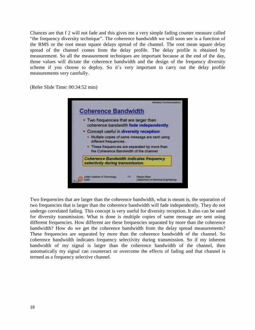
Chances are that f 2 will not fade and this gives me a very simple fading counter measure called
“the frequency diversity technique”. The coherence bandwidth we will soon see is a function of
the RMS or the root mean square delays spread of the channel. The root mean square delay
spread of the channel comes from the delay profile. The delay profile is obtained by
measurement. So all the measurement techniques are important because at the end of the day,
those values will dictate the coherence bandwidth and the design of the frequency diversity
scheme if you choose to deploy. So it‟s very important to carry out the delay profile
measurements very carefully.
(Refer Slide Time: 00:34:52 min)
Two frequencies that are larger than the coherence bandwidth, what is meant is, the separation of
two frequencies that is larger than the coherence bandwidth will fade independently. They do not
undergo correlated fading. This concept is very useful for diversity reception. It also can be used
for diversity transmission. What is done is multiple copies of same message are sent using
different frequencies. How different are these frequencies separated by more than the coherence
bandwidth? How do we get the coherence bandwidth from the delay spread measurements?
These frequencies are separated by more than the coherence bandwidth of the channel. So
coherence bandwidth indicates frequency selectivity during transmission. So if my inherent
bandwidth of my signal is larger than the coherence bandwidth of the channel, then
automatically my signal can counteract or overcome the effects of fading and that channel is
termed as a frequency selective channel.

19
(Refer Slide Time: 00:36:17 min)
Let us give some quantitative phase to the coherence bandwidth. If we define coherence
bandwidth given by B C as a range of frequencies over which the frequency correlation is 0.9,
clearly within the coherence bandwidth, the signal undergoes correlated fading. The signal is
correlated. So if the correlation is above 0.9 that is, the high degree of correlation then, B C is
given by 1/ 50 sigma tau. Sigma tau if you remember is the root mean square delay. This is a very
stringent definition. We can of course choose to relax the definition if we define the coherence
bandwidth as a range of frequencies over which the frequency correlation is above only 0.5.
Then it is a much broader coherence bandwidth. This is given by 1/5 sigma tau. In literature, both
are used but to be on the safer side we use B C as 1/ 5 sigma tau. This is the more popular
definition that is normally used.

20
(Refer Slide Time: 00:37:51 min)
Let us look at an example. Let us say for a certain multipath channel most likely an outdoor
multipath channel, the sigma tau is 1.37 ms. It is just an outdoor channel measurement. I do my
channel measurement. I obtain my power delay profile. I do my mathematics to find out the
sigma tau. It comes out to be 1.37 ms. we were interested in finding out the 50 % coherence
bandwidth for this channel. If you have to design a scheme which will overcome the effects of
fading, we need to separate it by more than the coherence bandwidth. Let us use the definition B
C = 1/5 sigma tau. In this case, if you plug in the value of sigma tau as 1.37 ms, the coherence
bandwidth comes out to be 146 KHz. that is, if my signal being used over this channel is larger
than 146 KHz, then automatically the fading effects can be overcome to some extent. Let‟s look
at for example. The old AMPS system which was deployed in the US. It is the analog mobile
phone systems. Since B C >30 KHz which is the band typically used for AMPS, I do not need to
use an equalizer for AMPS. Of course AMPS is no longer being used is the previous generation.
But if we are talking about GSM channel which is 200 KHz per channel, then we definitely
require an equalizer.
Conversation between Student and Professor: the question being asked is: for lower than the 50
%, we defined for this 0.9 coherence correlation and then 0.5 correlation which corresponds to
the 50 %. Typically we do not go below 50 % because then you are really uncorrelated. By
definition you are making the band larger and larger and you‟re going into the domain. So it is a
much looser calculation. You will be wasteful in your calculation. If you are using frequency
diversity, you need to have a larger bandwidth but you should use only as much frequency
separation as desired because most likely you will be sending the same signal over the two
frequency bands. Clearly if you separated too much, they will be uncorrelated but the game is to
find out the minimum separation required and if you go below 50 % to 20 % or so, clearly the
denominator will go down. The numerator will go up. So B C will become larger and larger. so it
doesn‟t save much. Normally it will not go below this 50 % definition.
21
(Refer Slide Time: 00:41:20 min)
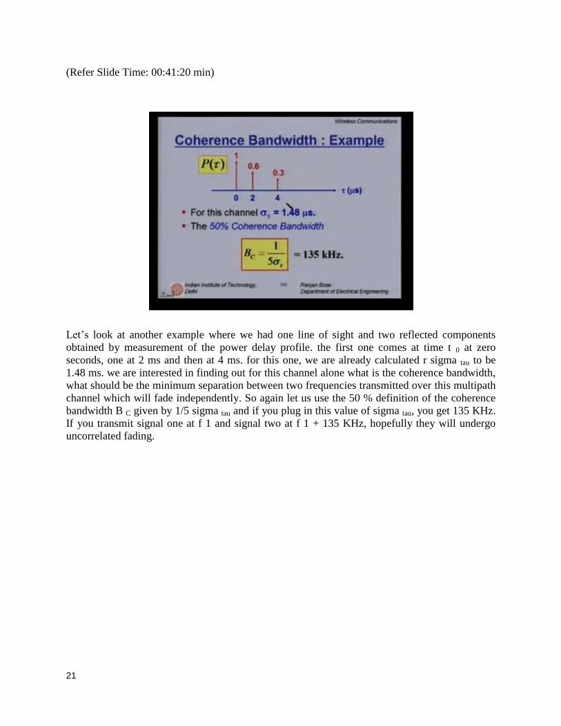
Let‟s look at another example where we had one line of sight and two reflected components
obtained by measurement of the power delay profile. the first one comes at time t 0 at zero
seconds, one at 2 ms and then at 4 ms. for this one, we are already calculated r sigma tau to be
1.48 ms. we are interested in finding out for this channel alone what is the coherence bandwidth,
what should be the minimum separation between two frequencies transmitted over this multipath
channel which will fade independently. So again let us use the 50 % definition of the coherence
bandwidth B C given by 1/5 sigma tau and if you plug in this value of sigma tau, you get 135 KHz.
If you transmit signal one at f 1 and signal two at f 1 + 135 KHz, hopefully they will undergo
uncorrelated fading.

22
(Refer Slide Time: 00:42:35 min)
Now let us look at a slightly different topic which is the coherence time issue and Doppler spread
related to the coherence time. We are talking about the temporal nature of the channel. So far
delay spread and which is clearly related to the coherence bandwidth describe only the time
dispersive nature of the multipath channel, that too in a local area. Clearly many times we
encounter mobile channels or even if the transmitter and receiver fixed relative to each other, we
find that the channel itself is changing. We experience something called as a Doppler shift that
has to be factored into the equations. The Doppler Spread and the coherence time which is
associated with the Doppler spread describe the time varying nature of the channel in a small
scale region. It is usually caused by the relative motion of the transmitter and receiver.

23
(Refer Slide Time: 00:43:50 min)
Let‟s capture this account. Let us take a brief look at the Doppler spread. we remember from our
previous lecture that if the mobile station is moving with a certain velocity „v‟, however signal is
impinged on the mobile station at an angle theta then, the „fd‟ the Doppler frequency spread is
given by the velocity divided by the wavelength times cosine theta. Please remember this lambda
wavelength plays an important part. The Doppler spread BD is nothing but the maximum
Doppler shift. So if the velocity goes up or down wavelength (check) is a whole range of
wavelengths used for communication. We are only talking about the maximum Doppler shift.
Clearly the Doppler shift depends on the relative velocity of the receiver with respect to the
transmitter and the wavelength of transmission. The angle „theta‟ at which the arriving signal
reaches the receiver also is important.
24
(Refer Slide Time: 00:45:04 min)
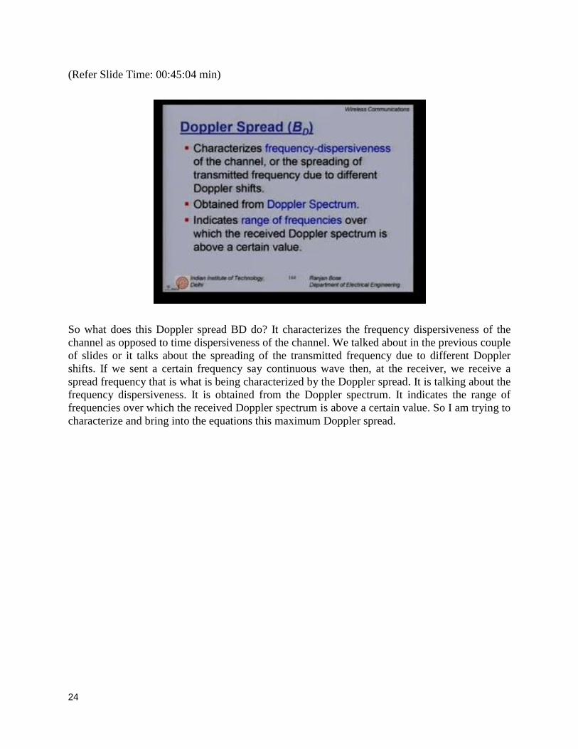
So what does this Doppler spread BD do? It characterizes the frequency dispersiveness of the
channel as opposed to time dispersiveness of the channel. We talked about in the previous couple
of slides or it talks about the spreading of the transmitted frequency due to different Doppler
shifts. If we sent a certain frequency say continuous wave then, at the receiver, we receive a
spread frequency that is what is being characterized by the Doppler spread. It is talking about the
frequency dispersiveness. It is obtained from the Doppler spectrum. It indicates the range of
frequencies over which the received Doppler spectrum is above a certain value. So I am trying to
characterize and bring into the equations this maximum Doppler spread.

25
(Refer Slide Time: 00:46:07 min)
So what we have seen already is that the Doppler spread „B D‟ is the maximum Doppler shift and
Doppler shift f D is velocity divided by wavelength times of cosine theta.
(Refer Slide Time: 00:46:24 min)
If the baseband signal bandwidth is much greater than „B D‟ - the maximum Doppler shift, in that
case the effects of the Doppler spread are negligible at the receiver. If such a case occurs then
this is a slow fading channel as opposed to a fast fading channel. It depends on the signal
bandwidth.

26
(Refer Slide Time: 00:47:00 min)
Let us now talk about the notion of a coherence time. coherence time is a statistical measure of
the time duration over which the channel impulse response is essentially time invariant if the
symbol period of the baseband signal is the reciprocal of the baseband signal bandwidth
approximately is greater than the coherence time. We are talking about a symbol period and the
coherence time is a symbol period is greater than the coherence time of the channel. Then the
channel will change during the transmission of the signal. Hence there will be distortions at the
receiver. The coherence time T C is defined as 1 over fm where fm is the maximum frequency
spread due to the Doppler shift and is earlier represented as P t. so it is a reciprocal of the
Doppler spread.

27
(Refer Slide Time: 00:48:15 min)
There are some popular thumb rules because in the previous slide, you saw that T C was only
approximately equal to 1 over f m transfer the maximum frequency spread. The popular thumb
rule is T C is given by under root 9/16 pi fm 2 which is nothing but 0.423 divided by f m. f m is the
maximum Doppler spread. This is popularly used. The definition of coherence time implies that
two signals arriving with a time separation greater than tau C are affected differently by the
channel. if you remember in the beginning of today‟s talk, we had projected one diagram which
was the two D mesh diagram. On one axis was the delay spread. On the other axis was the
measurement taken at different times. So this represents the second axis where the channel
changes with time. A large coherence time implies the channel changes slowly again. This is
related to the Doppler shift. If you are moving very fast in a vehicle, your channel will change
rapidly and that will be a fast fading scenario. Fast or slow depends on what is the symbol
duration whether the fading characteristics changes within a symbol interval or the fade can be
expected to be constant over several symbol intervals. That will decide whether it is fast fading
or slow fading scenario.
Our receiver systems in fading channels are designed taking into consideration whether the
channel is slowly fading or is a fast fading channel, whether it is a frequency flat channel
depending upon the coherence bandwidth or a frequency selective channel. So we have these
four things that have to be considered before you start designing a wireless communication
system.
28
(Refer Slide Time: 00:50:32 min)
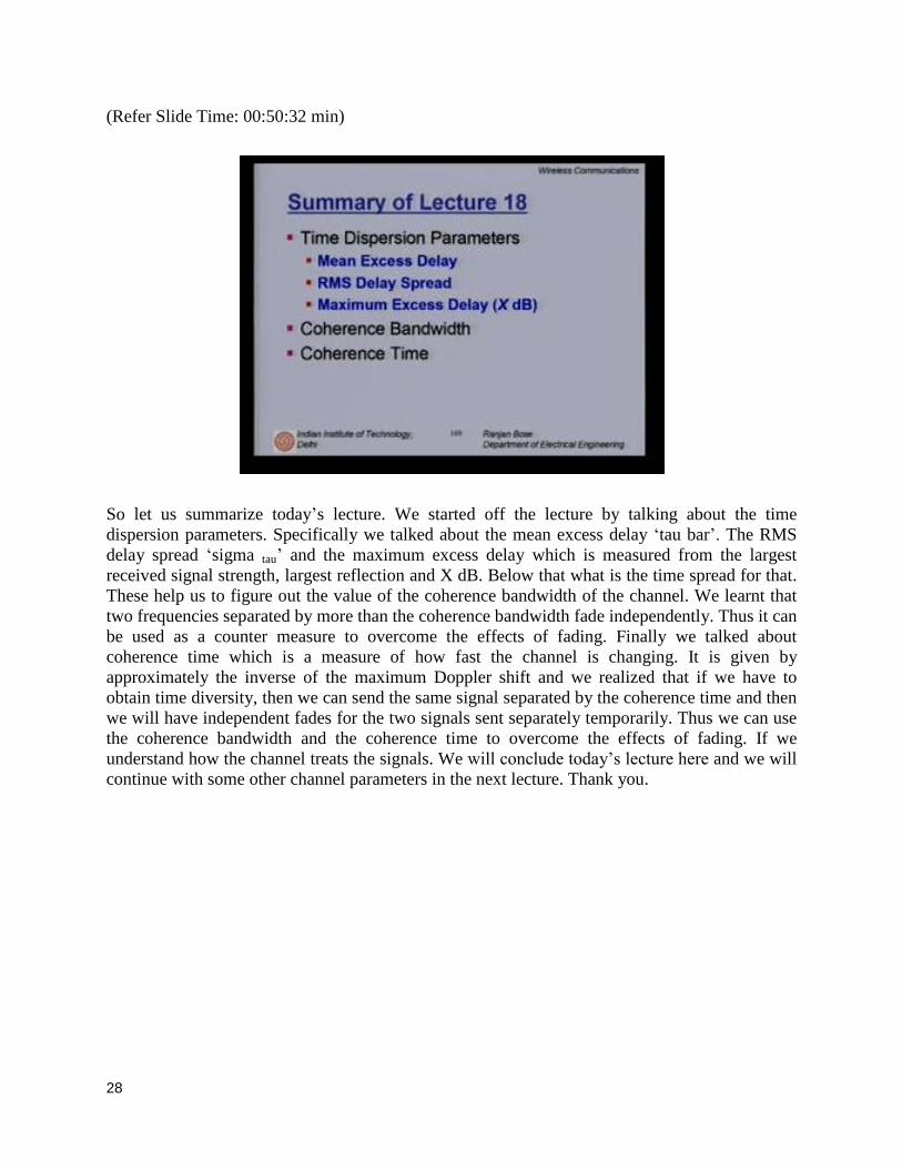
So let us summarize today‟s lecture. We started off the lecture by talking about the time
dispersion parameters. Specifically we talked about the mean excess delay „tau bar‟. The RMS
delay spread „sigma tau‟ and the maximum excess delay which is measured from the largest
received signal strength, largest reflection and X dB. Below that what is the time spread for that.
These help us to figure out the value of the coherence bandwidth of the channel. We learnt that
two frequencies separated by more than the coherence bandwidth fade independently. Thus it can
be used as a counter measure to overcome the effects of fading. Finally we talked about
coherence time which is a measure of how fast the channel is changing. It is given by
approximately the inverse of the maximum Doppler shift and we realized that if we have to
obtain time diversity, then we can send the same signal separated by the coherence time and then
we will have independent fades for the two signals sent separately temporarily. Thus we can use
the coherence bandwidth and the coherence time to overcome the effects of fading. If we
understand how the channel treats the signals. We will conclude today‟s lecture here and we will
continue with some other channel parameters in the next lecture. Thank you.