wireless communication - university of sydney · wireless communication system was then chosen and...
TRANSCRIPT

Wireless Communication for
High Speed Vehicle Project
Fayad Y. Tohme
This thesis has been undertaken as part of the course work required for the degree of
Bachelor of Engineering in Mechanical Engineering (Mechatronics)
Australian Centre for Field Robotics (ACFR) School of Aerospace, Mechanical and Mechatronic
Engineering The University of Sydney
November 2002
Declaration: The following is a list of work I carried out as part of the development of an autonomous road following system:
�� I declare that the work, ideas & codes in the following thesis are mine unless
they are quoted.
�� I declare that the Wireless communication package is chosen, bought and
implemented by me.
�� I designed and implemented the software for the Ute’s computer that reads
the Hyperkernel memory, receive messages and send messages through the
wireless network.
�� I designed and implemented the software for the Operator’s computer that
interface with the operator, send messages, and receive messages from the
wireless network and save data into the hard disk.
�� I designed, built and implemented the structure of the electromagnetic clutch
of the steering wheel.
�� I designed and build the circuit for the switching mechanism between the
Automatic and manual status of the car control.
Signed Eduardo Nebot (Supervisor)

Abstract: The Thesis is a part of the HSV Project at the Australian Centre for Field Robotic at the University of Sydney. The aim was to develop a wireless communication package to communicate between the Ute’s onboard computer and the operator’s computer. First all the sensors and actuators were studied and discussed, and all the important data that the operator would be interested in was analysed and specified. The wireless communication system was then chosen and developed. The band used was 2.4 GHz, using the IEEE 802.11b system by connecting the computers peek-to-peek. The wireless hardware package was carefully chosen such as: the Ute’s antenna, the operator’s antenna, the wireless communication Ethernet card and the Ethernet converter. The Communication library used was Msg_bus library where the connection was easily attached enabling the messages to be sent one at the time. Two main softwares were developed. The first software developed for the Ute reads all the sensors data from the Hyperkernel shared memory and sends it to the operator’s computer. The second software, the operator software communicates with the Ute, asks for specific data and saves it into text files. Finally, safety procedures for anyone planning to use the Ute were developed for people to follow while doing any sort of testing at any time.

Acknowledgments: Firstly, I would like to thank my supervisor, Ass. Prof. Eduardo Nebot, for his help
and guidance in every stage of this thesis. His support and keen interest in my
progress made this thesis possible.
I also want to express my appreciation to the entire HSV team – undergraduates and
post graduates – for the smooth team work conducted, in particular, Jose, Juan &
Trevor.
Lastly, I would like to offer my deepest gratitude and acknowledgement to my
family and friends for their support & encouragement, in particular Jihan &Toufic.

“To Mum & Dad” Thanks…

Abbreviations: ACFR: Australian Centre for Field Robotic. BPSK: Binary Phase Shift Keying. CCK: Complementary Code Keying. CCA: Clear Channel Assessment. DSSS: Direct Sequence Spread Spectrum. EIRP: equivalent isotropic radiated power. FHSS: Frequency Hopping Spread Spectrum. HiperLAN: High Performance European Radio LAN. HSV: High Speed Vehicle. INS: Inertial Navigation System. IP: Internet protocol. GPS: Global Positioning System. LAN: Local Area Network. MAC: Medium Access Control. OFDM: Orthogonal Frequency Digital Multiplexing. PC: Personal Computer. PLCP: Physical Layer Convergence Procedure. PMD: Physical Medium Dependent. PCI: Protocol Control Information. PDU: Protocol Data Unit. PHY: Physical Layer. QPSK: Quadrature Phase Shift Keying. RF: Radio Frequency. SDU: Service Data Unit. TCP: Transmission Control Protocol. WECAL: Wireless Ethernet Compatibility Alliance. WEP: Wired Equivalent Privacy. Wi-Fi: Wireless Fidelity. WLAN: Wireless Local Area Network. WPAN: Wireless Personal Area Networks. VPN: Virtual Private Networks.

Content Page: DECLARATION: _______________________________________________________________ I
ABSTRACT:___________________________________________________________________ II
ACKNOWLEDGMENTS: _______________________________________________________III
CONTENT PAGE:______________________________________________________________VI
LIST OF TABLES: _____________________________________________________________IX
LIST OF FIGURES: ____________________________________________________________IX
CHAPTER 1 ____________________________________________________________________ 1
1 INTRODUCTION __________________________________________________________ 1
1.1 HIGH SPEED VEHICLE (HSV) PROJECT BACKGROUND____________________________ 1 1.2 HSV SENSORS & ACTUATORS______________________________________________ 2 1.3 HSV SENSORS __________________________________________________________ 3
1.3.1 Differential GPS Unit__________________________________________________ 3 1.3.2 Inertial Navigation System ______________________________________________ 5 1.3.3 SICK Bearing Laser ___________________________________________________ 6 1.3.4 LVDT ______________________________________________________________ 7 1.3.5 Wheel Encoder _______________________________________________________ 7 1.3.6 Compass ____________________________________________________________ 8 1.3.7 Throttle Potentiometer _________________________________________________ 8 1.3.8 Brake Potentiometer___________________________________________________ 9
1.4 ACTUATOR & CONTROLLER _______________________________________________ 9 1.4.1 Steering Actuator & Controllers _________________________________________ 9 1.4.2 Throttle Actuator & Control____________________________________________ 11 1.4.3 Brake Actuator & Control _____________________________________________ 12 1.4.4 Data Transfer _______________________________________________________ 13
CHAPTER 2 ___________________________________________________________________ 14
2 WIRELESS COMMUNICATIONS: __________________________________________ 14
2.1 INTRODUCTION ________________________________________________________ 14 2.1.1 Bluetooth __________________________________________________________ 14 2.1.2 WDCT_____________________________________________________________ 15

2.1.3 HomeRF ___________________________________________________________ 15 2.1.4 802.11b____________________________________________________________ 15 2.1.5 802.11a____________________________________________________________ 16 2.1.6 HiperLAN __________________________________________________________ 16
2.2 IEEE 802.11.B_________________________________________________________ 16 2.2.1 Terminology: _______________________________________________________ 17 2.2.2 Features: __________________________________________________________ 18 2.2.3 Implementations: ____________________________________________________ 18
2.3 WIRELESS LOCAL AREA NETWORK _________________________________________ 19 2.4 WLAN CONFIGURATION _________________________________________________ 20
2.4.1 Peer-to-peer (ad hoc mode) ____________________________________________ 20 2.4.2 Client/server (infrastructure networking) _________________________________ 21 2.4.3 Selection ___________________________________________________________ 22
2.5 AIM FOR THE WIRELESS COMMUNICATION ___________________________________ 22
CHAPTER 3 ___________________________________________________________________ 23
3 HARDWARE _____________________________________________________________ 23
3.1 STRUCTURE ___________________________________________________________ 23 3.2 ANTENNAS____________________________________________________________ 24
3.2.1 Gaining coverage range: ______________________________________________ 24 3.2.2 Positioning antennas:_________________________________________________ 24
3.3 UTE ANTENNA _________________________________________________________ 25 3.3.1 Specifications _______________________________________________________ 25
3.4 OPERATOR ANTENNA ___________________________________________________ 25 3.4.1 Specifications _______________________________________________________ 26
3.5 WIRELESS NETWORK CARD_______________________________________________ 26 3.5.1 Silver Label Cards Features____________________________________________ 26 3.5.2 Compatibility _______________________________________________________ 27
3.6 ETHERNET CONVERTER __________________________________________________ 28 3.7 DATA PROTECTION AND SECURITY _________________________________________ 28 3.8 RANGE DETECTION:_____________________________________________________ 29 3.9 RANGE TROUBLESHOOTING: ______________________________________________ 30
CHAPTER 4 ___________________________________________________________________ 32
4 LIBRARY FUNCTION _____________________________________________________ 32
4.1 BACKGROUND: ________________________________________________________ 32 4.2 MESSAGE BUS FUNCTIONS: _______________________________________________ 32
4.2.1 Attached: __________________________________________________________ 33

4.2.2 Detach:____________________________________________________________ 33 4.2.3 Sending: ___________________________________________________________ 34 4.2.4 Receiving:__________________________________________________________ 35
4.3 URGENT MESSAGES _____________________________________________________ 36
CHAPTER 5 ___________________________________________________________________ 38
5 SOFTWARE DEVELOPMENT ______________________________________________ 38
5.1 INTRODUCTION ________________________________________________________ 38 5.2 REQUIREMENTS ________________________________________________________ 39 5.3 DESIGN ______________________________________________________________ 40
5.3.1 The Ute’s Software ___________________________________________________ 41 5.3.2 The Operator’s Software ______________________________________________ 43
5.4 CODING ______________________________________________________________ 45 5.4.1 The Ute’s code ______________________________________________________ 45 5.4.2 The Operator’s Software ______________________________________________ 48
5.5 TESTING & MAINTENANCE _______________________________________________ 54
CHAPTER 6 ___________________________________________________________________ 56
6 SAFETY _________________________________________________________________ 56
6.1 AIMS ________________________________________________________________ 56 6.2 OCCUPATIONAL HEALTH AND SAFETY POLICY ________________________________ 56 6.3 HSV PROJECT SAFETY __________________________________________________ 57 6.4 SAFETY PROCEDURES ___________________________________________________ 57 6.5 PROCEDURES: WHEN ACCIDENTS HAPPEN ___________________________________ 58 6.6 WAVELAN AND YOUR HEALTH ___________________________________________ 59 6.7 CONCLUSION __________________________________________________________ 60
CHAPTER 7 ___________________________________________________________________ 61
7 CONCLUSION ____________________________________________________________ 61
7.1 FUTURE WORK & IMPLEMENTATION:________________________________________ 61
REFERENCES: ________________________________________________________________ 63
APPENDIX A: _________________________________________________________________ 64
List of Tables: Table 3-1: Range Detection ................................................................................................................ 30 Table 5-1: Sensors Timing .................................................................................................................. 39
List of Figures: Figure 1-1: Differential GPS ________________________________________________________ 4 Figure 1-2: SICK Laser ____________________________________________________________ 6 Figure 1-3: Wheel Encoder _________________________________________________________ 7 Figure 1-4: Steering Actuator _______________________________________________________ 9 Figure 1-5: System Control ________________________________________________________ 11 Figure 2-0-1: Peer-to-Peer ________________________________________________________ 20 Figure 2-0-2: Software Access Point _________________________________________________ 21 Figure 3-0-1: Wireless Communication Hardware ______________________________________ 23 Figure 3-0-2: Orinoco Wireless Ethernet Card _________________________________________ 27 Figure 3-3: Ethernet Converter Hardware ____________________________________________ 28 Figure 5-1: Software Development Stages_____________________________________________ 38 Figure 5-2: Main Software Architecture ______________________________________________ 40 Figure 5-3: Ute's Software Architecture ______________________________________________ 42 Figure 5-4: Operator's Software Architecture __________________________________________ 44
Chapter 1 Introduction 1
Chapter 1
1 Introduction
1.1 High Speed Vehicle (HSV) Project background The High Speed Vehicle (HSV) project has been a successful ongoing project
conducted by the Australian Centre for Field Robotics (ACFR) since 1997. The
primary objective of past undergraduate students and researchers in the project has
been the development of navigation and control algorithms to enable autonomously
autonomous operations of land vehicle operating in unknown environments. The
experimental prototype consists of a Holden S-series Commodore Utility car that is
retrofitted with a large number of sensors, actuators, data logging and control
system.
The aim of the HSV project is to develop technologies for the automation of a land
vehicle operating at ‘high speed’ (speed up to 90 Km/h) in a variety of ‘real’
environments. The Project is funded by ACFR and CMTE.
The ‘high speed’ element increases system complexity, requiring the vehicle to look
further ahead. This necessitates the consideration of a multitude of future motion
outcomes - all of which need to be implemented within a software architecture
possessing multiple layers of redundancy and ‘safe’ failure modes.
Chapter 1 Introduction 2
To make such systems a reality, the HSV project researches all aspects of automated
vehicle navigation. This process can be broken down into four steps:
1) Perceiving and modelling the environment.
2) Localising the vehicle within its environment.
3) Planning and deciding the vehicle’s desired motion.
4) Executing the vehicle’s desired motion.
Developing robust and reliable control systems required by an autonomous vehicle
for high speed operation (in often unstructured, real-world environments) is a
challenging task. Techniques and algorithms implemented on low speed (often
indoor) mobile robots working in static, structured environments are often
inappropriate for a high speed autonomous vehicle. Research in new sensors and
perception algorithm is essential for reliable navigation in all terrain applications.
The ultimate goal of this project is to be able to design a system capable of
determining the location of the vehicle in unstructured and unknown environments
and to be able to control it to perform a desired path with cm accuracy.
1.2 HSV Sensors & Actuators Research and development work is tested, debugged, evaluated and implemented on
the HSV project’s test vehicle, a mid-1990’s Holden utility (‘Ute’), retorted with the
computing, sensing and actuation hardware necessary for complete automation. A
PC (Pentium II, 400MHz, 64MB RAM) running the MS Windows NT (with the
Hyperkernel real-time extension) and QNX (real-time) operating system is located
in the Ute's tray, along with data acquisition equipment (such as an A/D converter)
for interfacing between the sensors and actuators. Inside the cabin, on the
passenger’s side, a screen monitor has been mounted, to facilitate monitoring of
system performance during testing.
A substantial suite of sensors is currently available for use on the ‘Ute’, providing
several potential localisation and environmental sensing options and configurations.
The sensors implemented are outlined as follows:
Differential GPS Unit, Inertia Navigation System (INS), SICK Bearing Laser,

Chapter 1 Introduction 3
LVDT, Wheel Encoder, MM-Radar, Compass, Panoramic Vision, Throttle
Potentiometer, Brake Potentiometer.
Three actuation systems (for steering, throttle and brake) are also in place, allowing
the Ute to operate under complete autonomous control. A brief description of the
configuration of these three systems is now given:
�� Steering Actuator & Control: a DC motor, mounted inside the driver’s foot-
well, turns the steering column through a worm reduction gearbox and an
electromagnetic clutch
�� Throttle Actuator & Control: a linear actuator controls the displacement of
the carburettor butterfly valve (which determines engine power output), via a
guide cable.
�� Brake Actuator & Control: a second linear actuator (mounted under the
driver’s seat) controls the position of the brake pedal directly. The physical
connection between the pedal and the actuator is via two cables, threaded
through a bracket in the front of the foot-well.
1.3 HSV Sensors A substantial suite of sensors is currently available for use on the ‘Ute’, these
providing several potential localization and environmental sensing options and
configurations. The following part of this chapter will list and describe the sensors
used in the Ute. Furthermore, the wirelessly transferred data structures produced by
each sensor are also provided with a brief explanation.
1.3.1 Differential GPS Unit The Global Positioning System or GPS is a unit which can provide position and
velocity information. Using a series of satellites orbiting the Earth, in known orbits,
the unit can determine where and what heading the unit is travelling. The system on
the HSV is called a differential GPS, which will return higher accuracy to the data
received. A base station is set up at a known geographical location, and taking the
GPS information received at this station, an estimate of the GPS error can be made.
This error is then sent, via radio, to the HSV computer which then removes the
estimated error from the GPS information gathered from the GPS unit located on it.

Chapter 1 Introduction 4
The information gathered from such a system provides a global position in the
North, East and Down (vertical elevation), as well as the unit’s velocities in these
frames. These are the main six data values used, but other information on the GPS
system is also provided, such as the number of satellites transmitting to the unit and
the variance of the individual signals.
Figure 1-1: Differential GPS
The wirelessly transferred data:
timestamp; // timestamp (in milliseconds) using GPS
latitude; // latitude (in degrees)
longitude; // longitude (in degrees)
altitude; // altitude (in metres)
ttcourse; // track/true course (in degrees)
speedog; // speed over ground (in knots)
vspeed; // vertical speed (metres/sec)
sigmaLati; // Sigma latitude
sigmaLongi; // Sigma longitude
sigmaAlti; // Sigma altitude
mode; // GPS mode
satellites; // number of satellites

Chapter 1 Introduction 5
1.3.2 Inertial Navigation System INS Stands for "Inertial Navigation System". It is a black box (literally!) containing
a combo of sensors. It consists of gyros, accelerometers and inclinometers arranged
along 3 perpendicular axes.
�� Gyros measure angular velocity, so we can measure how fast the Ute is
turning and tilting.
�� Accelerometers measure acceleration. This lets us know how fast the car is
accelerating or decelerating in any direction.
�� Inclinometers measure inclination. This lets us know if the Ute is tilting or
banking.
This provides data in all six degrees of freedom: acceleration and angular velocity in
all three axes, with bank and elevation angles from the pendulum gyroscopes. This is
used to provide dead-reckoning estimation of the HSV’s position, through
integration of the acceleration and angular velocity to provide position and heading.
The wirelessly transferred data:
timestamp; // timestamp (in milliseconds)
bank; // bank
elev; // elevation
ax; // acceleration along x-axis
ay; // acceleration along y-axis
az; // acceleration along z-axis
gx; // angular acc. about x-axis
gy; // angular acc. about y-axis
gz; // angular acc. about z-axis

Chapter 1 Introduction 6
1.3.3 SICK Bearing Laser To obtain a picture of the environment around the HSV, a bearing laser was situated
at the front of the HSV. The basis of the bearing laser is that it emits a single infra-
red laser pulse which is reflected back from any object within its vicinity. The time
that the beam takes to return to the unit is measured, and then using the speed of
light, the distance that the object is away from the bearing laser can be calculated.
An image of the environment is then constructed by rotating the laser and taking
samples at known angular intervals.
Figure 1-2: SICK Laser
For this SICK Bearing laser range samples are taken at every 0.5°, for a range of
180° and a distance of up to 80m. The data given for each sweep of the sensor is in
the format of a range reading for every sample taken, thus a total of 361 range
readings. This model also provides the intensity of the return signal, which is
presented in the same format. This feature is useful for identifying markers and
reflective objects.
The wirelessly transferred data:
timestamp; // timestamp (in milliseconds)
range[i]; //Laser Range 180o for 360 section

Chapter 1 Introduction 7
1.3.4 LVDT An LVDT is a measurement device which uses the electromagnetic force that is
induced in the movement of a ferrous core through two electromagnetic coils. The
LVDT uses this principle to measure linear movement, by attaching the two ends to
the linear distance needed to be measured. For the HSV, this has been attached to the
steering system of the Ute, and returns a value of the angle the vehicle’s steering has
shifted.
To prevent any physical damage to the steering hardware, a certain range of steering
angle has been given as a default so that the actuators are not forced to drive the
steering rack past its physical limits.
The wirelessly transferred data:
Steering ; // Steering Sensor LVDT Value real_steering_output; // The Real Steering Output (Calculated)
1.3.5 Wheel Encoder The ROD-430 wheel encoder is incremental rotary velocity encoders from
Heidenhain. The encoders operate on the principle of photo electrically scanning
very fine grating with a line counts between 50 to 5000. The shaft attaching to the
wheel encoders can oscillate up to 12 000 rpm. Output signals for this particular
model are HTL square-wave signals, therefore incorporating a circuit which
digitizes sinusoidal scanning signals, providing two 90 deg phase-shifted pulse
trains and a reference pulse. The encoder is powered by the 12 Vdc from the fuse
box.
Figure 1-3: Wheel Encoder
The wirelessly transferred data:
Counts; // The Potentiometer counting value
Chapter 1 Introduction 8
1.3.6 Compass An alternative source of vehicle heading information is measured relative to
magnetic north. The compass used was TCM2. The TCM2's elimination of a
mechanical gimbal is unique among electronic compasses. All compasses must be
referenced to level in order to be accurate, so instead of using a clumsy universal
joint or fluid bath to hold its sensors level, the TCM2 uses a highly accurate
inclinometer (tilt sensor) to allow the microprocessor to mathematically correct for
tilt. This electronic gimbaling eliminates moving parts and provides more
information about the environment: pitch and roll angles and three dimensional
magnetic field measurements in addition to compass output. This extra data allows
the TCM2 to provide greater accuracy in the field by calibrating for distortion fields
in all tilt orientations, providing an alarm when local magnetic anomalies are
present, and giving out-of-range warnings when the unit is being tilted too far.
The wirelessly transferred data:
timestampB ; // timestamp (in milliseconds)
Heading; // latitude (in degrees)
Pitch; // longitude (in degrees)
Roll; // altitude (in metres)
1.3.7 Throttle Potentiometer For throttle control, the feedback of the throttle position is obtained from a
potentiometer that was built into the linear actuator. The potentiometer consists of a
voltage divider where the potentiometer output wiper moves with the actuator rod.
the potentiometer reads from 1000 ohms to 11000 ohms and its output voltage range
is given by the two voltages (Vpot- & Vpot+) applied at the extremities of the
potentiometer resistor. The voltages applied at the two extremities are (-8.6V &
+8.6V) and therefore the voltage range of the potentiometer is (-8.6V & +8.6V).
The throttle moves with the actuator rod until the former reaches either of its
minimum or maximum positions. Therefore, in the active region, i.e. the region
where the throttle moves with the actuator rod, the distance moved by the actuator
rod is also the distance moved by the throttle & therefore the voltage reading from
the potentiometer is also proportional to the throttle position.

Chapter 1 Introduction 9
The wirelessly transferred data:
Accelerator; // the Acceleration Sensor Value
1.3.8 Brake Potentiometer For throttle control, the feedback of the throttle position is obtained from a
potentiometer that was built into the linear actuator. The potentiometer consists of a
voltage divider where the potentiometer output wiper moves with the actuator rod.
The potentiometer reads from 0 ohms to 1000 ohms and its output voltage range are
given by the two voltages (Vpot- & Vpot+) applied at the extremities of the
potentiometer resistor. The voltages applied at the two extremities are (-8.6V &
+8.6V) and therefore the voltage range of the potentiometer is (-8.6V & +8.6V). The
Brake Pedal moves with the actuator rod until the former reaches either of its
minimum or maximum positions.
The wirelessly transferred data:
Brake; // The Brake Sensor Value
1.4 Actuator & Controller
1.4.1 Steering Actuator & Controllers The steering in the HSV can be actuated in two ways: Manual or Automatic. A DC
motor is used to drive through a worm reduction gearbox onto the steering
mechanism to be able to turn left and right at a variable speed.
Figure 1-4: Steering Actuator
Components: Motor:
Power: 120 W
Voltage: 24 V
Current: 5A
Rated Speed: 2000 rpm (209 rad/s)
Chain
Clutch
Worm Gearbox
DC Motor
Gearbox:
Type: Worm Reduction
Rotation: 90o

Chapter 1 Introduction 10
Ratio: 40:1
Efficiency: 90% (not accurate)
Torque:
Torque Required: 8 Nm
Motor Torque = Power / Rated Speed = P / W = 120/209 = 0.5742 Nm
Torque Generated by the Gearbox = Efficiency * Motor Torque * Ratio
= 0.9 * 0.5742 * 40 = 20.699 Nm
Therefore the Motor / Gearbox will generate enough torque for the steering.
Clutch:
The clutch that is used is a Lenze 10 Nm electromagnetic clutch. An electromagnetic
clutch was used to be able to switch the car using one single button from
autonomous mode to manual mode
Engagement:
Electromechanical clutches operate via an electric actuation, but transmit torque
mechanically. When the clutch is required to actuate, voltage/current is applied to
the clutch coil. The coil becomes an electromagnet and produces magnetic lines of
flux. This flux is then transferred through the small air gap between the field and the
rotor. The rotor portion of the clutch becomes magnetized and sets up a magnetic
loop that attracts the armature. The armature is pulled against the rotor and a
frictional force is applied at contact. Within a relatively short time the load is
accelerated to match the speed of the rotor, thereby engaging the armature and the
output hub of the clutch. In most instances, the rotor is constantly rotating with the
input all the time.
Disengagement:
When current/voltage is released from the clutch, the armature is free to turn with
the shaft. In most designs, springs hold the armature away from the rotor surface
when power is released; creating a small space that enables the two parts to rotate.
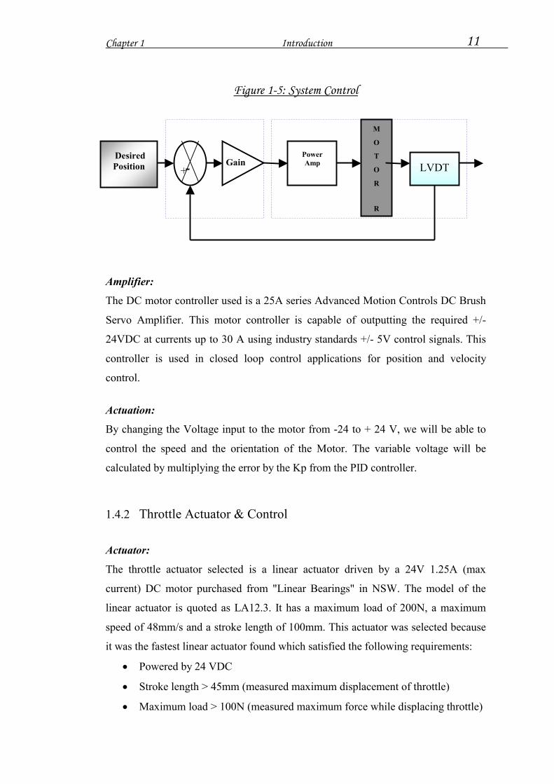
System Control The LVDT reads the position of the steering rack and a voltage signal is taken as the
feedback value. The error between this value and the set point is evaluated and the
control algorithm determines a new output for the steering actuator.
Chapter 1 Introduction 11
Figure 1-5: System Control
LVDT
M
O
T
O
R
R
Power Amp Gain
+ - Desired Position
Amplifier:
The DC motor controller used is a 25A series Advanced Motion Controls DC Brush
Servo Amplifier. This motor controller is capable of outputting the required +/-
24VDC at currents up to 30 A using industry standards +/- 5V control signals. This
controller is used in closed loop control applications for position and velocity
control.
Actuation:
By changing the Voltage input to the motor from -24 to + 24 V, we will be able to
control the speed and the orientation of the Motor. The variable voltage will be
calculated by multiplying the error by the Kp from the PID controller.
1.4.2 Throttle Actuator & Control
Actuator:
The throttle actuator selected is a linear actuator driven by a 24V 1.25A (max
current) DC motor purchased from "Linear Bearings" in NSW. The model of the
linear actuator is quoted as LA12.3. It has a maximum load of 200N, a maximum
speed of 48mm/s and a stroke length of 100mm. This actuator was selected because
it was the fastest linear actuator found which satisfied the following requirements:
�� Powered by 24 VDC
�� Stroke length > 45mm (measured maximum displacement of throttle)
�� Maximum load > 100N (measured maximum force while displacing throttle)

Chapter 1 Introduction 12
Control Mechanical System:
For throttle control, the mechanical system consists mainly of a linear actuator and
guided cables (the same cables used to link the accelerator pedal & throttle). When
the actuator rod reacts, it pulls the cable along with it. This increases the extent at
which the throttle valve is opened and hence increases the acceleration of the
vehicle. As the actuator rod extends, the cable tension reduces and slackens,
allowing the returning spring at the throttle to return towards its original
(undisplaced) position. This reduces the throttle valve opening and hence reduces
the acceleration of the vehicle.
1.4.3 Brake Actuator & Control
Actuator:
The throttle actuator selected is a linear actuator driven by a 24V 6A (max current)
DC motor purchased from "Linear Bearings" in NSW. The model of the linear
actuator is quoted as LA30.3. It has a maximum load of 1500N, a maximum speed
of 42mm/s and a stroke length of 150mm. This actuator was selected because it was
the fastest linear actuator found which satisfied the following requirements:
�� Powered by 24 VDC
�� Stroke length > 100mm (measured maximum displacement of brake pedal)
�� Maximum load > 500N (measured maximum force while displacing brake
pedal) Control Mechanical System:
For brake control, the mechanical system consists mainly of a linear actuator and
guided cables (the same cables used to link the accelerator pedal & throttle). When
the actuator rod retracts, it pulls the cable along with it, thereby pulling the brake
pedal further which causes an increase in the braking force on the vehicle. As the
actuator rod extends, the restoring spring at the brake pedal restores the brake pedal
towards the undisplaced position thereby reducing the braking force on the vehicle.
Chapter 1 Introduction 13
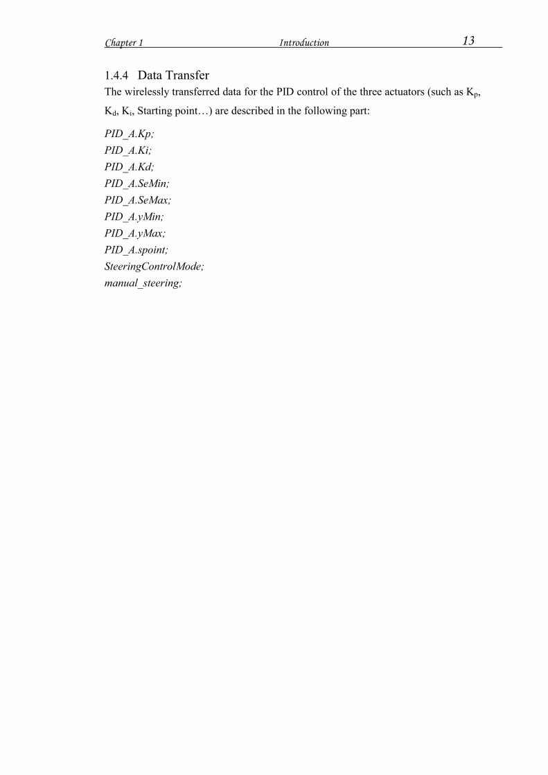
1.4.4 Data Transfer The wirelessly transferred data for the PID control of the three actuators (such as Kp,
Kd, Ki, Starting point…) are described in the following part:
PID_A.Kp; PID_A.Ki; PID_A.Kd; PID_A.SeMin; PID_A.SeMax; PID_A.yMin; PID_A.yMax; PID_A.spoint; SteeringControlMode; manual_steering;

Chapter 2 Wireless Communications: 14
Chapter 2
2 Wireless Communications:
2.1 Introduction Wireless communications persist to encapsulate exponential growth in the cellular
telephony, wireless networking and internet territories. The number of wireless
subscribers worldwide has transcended from 425 million in 1999 to 953 million in
late 2002. At present, two types of wireless standards are gaining tremendous
industry share and interest due to their operative functionalities and characteristics,
namely the Bluetooth system and the IEEE 802.11 system. It is important to note
however, that a diversity of other wireless systems such as WDCT, Hiperlan/21 and
HomeRF2 also exist and have a small piece of the marketplace. The IEEE 802.11b
system was used for the Wireless networking between the operator and the Ute
onboard computer.
2.1.1 Bluetooth Bluetooth is an open wireless standard which utilizes the unlicensed 2.4 GHz
Industrial-Scientific-Medical (ISM) band for short distance transmissions. At a
maximum data rate of 1 Mbps, it transfers voice and data wirelessly in Wireless
Personal Area Networks (WPANs) using Frequency Hopping Spread Spectrum
(FHSS) modulation scheme. Bluetooth is backed by the Bluetooth Special Interest
Group (SIG), which has support from industry leaders including Motorola, IBM,
Intel, Nokia, Toshiba, Ericsson, and 3Com. (Enos, L. 2000)

Chapter 2 Wireless Communications: 15
2.1.2 WDCT The DECT (Digital Enhanced Cordless Telecommunication) standard which
originated as a European initiative was not adopted as a worldwide wireless
telecommunications standard. Following years of success with DECT in Europe,
Africa and South America, the WDCT (Worldwide Digital Cordless
Telecommunications) standard was specifically developed for the North American
market in 1998. Operating in the 2.4 GHz frequency band, WDCT has adopted the
FHSS modulation scheme with a 1,000-foot transmission range and voice quality
that is comparable to fixed networks. (Enos, L. 2000)
2.1.3 HomeRF HomeRF is a wireless technology that combines the voice protocol from DECT with
the data transfer technique in 802.11b. It operates in the 2.4 GHz frequency band at
10 Mbps peak data rate, providing a range of up to 150 feet while utilizing the FHSS
frequency modulation method. The HomeRF Working Group Inc. (HRFWG) was
formed to ensure the interoperability of wireless devices in distributing voice, data
and streaming media in consumer environments. Key members include: Intel,
Motorola, Compaq and Siemens. (Enos, L. 2000)
2.1.4 802.11b The 802.11b standard was established by the Institute of Electrical and Electronic
Engineers (IEEE), while the Wireless Compatibility Ethernet Alliance (WECA)
ensures that all 802.11b products are interoperable. 802.11b, also known as Wi-Fi™,
operates at 2.4 GHz with a maximum bandwidth of 11 Mbps while 802.11b WLANs
provide ranges up to 300 feet. Unlike other wireless standards in the 2.4 GHz
frequency band, 802.11b has adopted the Direct Sequence Spread Spectrum (DSSS)
frequency modulation scheme. Major WECA members include Cisco, Lucent and
Nokia.

Chapter 2 Wireless Communications: 16
2.1.5 802.11a 802.11a is a wireless standard that operates in the 5.15 ~ 5.35 GHz and 5.725 ~
5.825 GHz frequency bands. 802.11a was developed by the IEEE as a
complementary technology to 802.11b under WECA. To achieve a 54 Mbps peak
transmission rate, 802.11a uses Orthogonal Frequency Digital Multiplexing
(OFDM) modulation scheme. 802.11a WLANs can transmit as far as 400 feet.
2.1.6 HiperLAN HiperLAN (High Performance European Radio LAN) technology, which was
developed by the European Telecommunications Standard Institute, operates in the
5.15 ~ 5.25 GHz and 5.470 ~ 5.725 GHz frequency bands with QoS support. With a
peak data rate of 54 Mbps, HiperLAN also utilizes the OFDM frequency modulation
method for data transmissions. Like 802.11a, HiperLAN is capable of achieving a
400-foot transmission range. An open forum, HiperLAN2, was established to be a
global standard with complete interoperability of high-speed wireless LAN products.
Key members include Sony, Nortel Networks, Nokia, and STMicroelectronics.
(Pahlavan, K. 1995)
2.2 IEEE 802.11.b The IEEE 802.11.b was the wireless system used in the project because it is the most
convenient, the cheapest, and the easiest to implement, and it was available. The
IEEE 802.11.b standard specifies a 2.4 GHz operating frequency with data rates of 1
and 2 Mbps using either direct sequence (DSSS) or frequency hopping spread
spectrum (FHSS). IEEE 802.11b data is encoded using DSSS (Direct Sequence
Spread Spectrum) technology. DSSS works by taking a data stream of zeros and
ones and modulating it with a second pattern, the chipping sequence.
In 802.11, that sequence is known as the Barker code, which is an 11-bit sequence
(10110111000) that has certain mathematical properties making it ideal for
modulating radio waves. The basic data stream XOR’d with the Barker code
generates a series of data objects called chips. Each bit is "encoded" by the 11 bit
Barker code, and each group of 11 chips encodes one bit of data.

Chapter 2 Wireless Communications: 17
The CCK (Complementary Code Keying) achieves 11 Mbps. Rather than using the
Barker code, CCK uses a series of codes called Complementary Sequences. Because
there are 64 unique code words that can be used to encode the signal, up to 6 bits can
be represented by any one particular code word (instead of the 1 bit represented by a
Barker symbol).
The wireless radio generates a 2.4 GHz carrier wave (2.4 to 2.483 GHz) and
modulates that wave using a variety of techniques. For 1 Mbps transmission, BPSK
(Binary Phase Shift Keying) is used (one phase shift for each bit). To accomplish 2
Mbps transmission, QPSK (Quadrature Phase Shift Keying) is used. QPSK uses four
rotations (0, 90, 180 and 270 degrees) to encode 2 bits of information in the same
space as BPSK encodes 1. The trade-off is increase power or decrease range to
maintain signal quality. Because the FCC regulates output power of portable radios
to 1 watt EIRP (equivalent isotropic radiated power), range is the only remaining
factor that can change. On 802.11 devices, as the transceiver moves away from the
radio, the radio adapts and uses a less complex (and slower) encoding mechanism to
send data. (Gast, M. 2002)
2.2.1 Terminology: The MAC layer communicates with the PLCP via specific primitives through a PHY
service access point. When the MAC layer instructs, the PLCP prepares MPDUs for
transmission. The PLCP also delivers incoming frames from the wireless medium to
the MAC layer. The PLCP sublayer minimizes the dependence of the MAC layer on
the PMD sub layer by mapping MPDUs into a frame format suitable for
transmission by the PMD. Under the direction of the PLCP, the PMD provides
actual transmission and reception of PHY entities between two stations through the
wireless medium.
To provide this service, the PMD interfaces directly with the air medium and
provides modulation and demodulation of the frame transmissions. The PLCP and
PMD communicate using service primitives to govern the transmission and
reception functions.

Chapter 2 Wireless Communications: 18
2.2.2 Features: The CCK code word is modulated with the QPSK technology used in 2 Mbps
wireless DSSS radios. This allows for an additional 2 bits of information to be
encoded in each symbol. Eight chips are sent for each 6 bits, but each symbol
encodes 8 bits because of the QPSK modulation. The spectrum math for 1 Mbps
transmission works out as 11 Mchips per second times 2 MHz equals 22 MHz of
spectrum. Likewise, at 2 Mbps, 2 bits per symbol are modulated with QPSK, 11
Mchips per second, and thus have 22 MHz of spectrum. To send 11 Mbps, 22MHz
of frequency spectrum is needed. It is much more difficult to discern which of the 64 code words is coming across the
airwaves, because of the complex encoding. Furthermore, the radio receiver design
is significantly more difficult. In fact, while a 1 Mbps or 2 Mbps radio has one
correlator (the device responsible for lining up the various signals bouncing around
and turning them into a bit stream), the 11 Mbps radio must have 64 such devices.
(Gast, M. 2002)
2.2.3 Implementations: The wireless physical layer is split into two parts, called the PLCP (Physical Layer
Convergence Protocol) and the PMD (Physical Medium Dependent) sublayer. The
PMD takes care of the wireless encoding explained above. The PLCP presents a
common interface for higher-level drivers to write to and provides carrier sense and
CCA (Clear Channel Assessment), which is the signal that the MAC (Media Access
Control) layer needs so it can determine whether the medium is currently in use.
The PLCP consists of a 144 bits preamble that is used for synchronization to
determine radio gain and to establish CCA. The preamble comprises 128 bits of
synchronization, followed by a 16 bits field consisting of the pattern
1111001110100000. This sequence is used to mark the start of every frame and is
called the SFD (Start Frame Delimiter). The next 48 bits are collectively known as
the PLCP header. The header contains four fields: signal, service, length and HEC
(header error check). The signal field indicates how fast the payload will be
transmitted (1, 2, 5.5 or 11 Mbps). The service field is reserved for future use. The
length field indicates the length of the ensuing payload, and the HEC is 16 bits CRC
Chapter 2 Wireless Communications: 19
of the 48 bits header.
In a wireless environment, the PLCP is always transmitted at 1 Mbps. Thus, 24
bytes of each packet are sent at 1 Mbps. The PLCP introduces 24 bytes of overhead
into each wireless Ethernet packet before we even start talking about where the
packet is going. Ethernet introduces only 8 bytes of data. Because the 192 bits
header payload is transmitted at 1 Mbps, 802.11b is at best only 85 percent efficient
at the physical layer. (Gast, M. 2002)
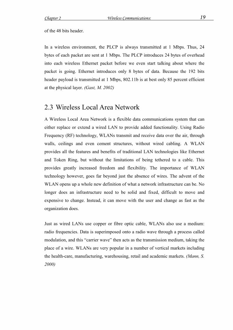
2.3 Wireless Local Area Network A Wireless Local Area Network is a flexible data communications system that can
either replace or extend a wired LAN to provide added functionality. Using Radio
Frequency (RF) technology, WLANs transmit and receive data over the air, through
walls, ceilings and even cement structures, without wired cabling. A WLAN
provides all the features and benefits of traditional LAN technologies like Ethernet
and Token Ring, but without the limitations of being tethered to a cable. This
provides greatly increased freedom and flexibility. The importance of WLAN
technology however, goes far beyond just the absence of wires. The advent of the
WLAN opens up a whole new definition of what a network infrastructure can be. No
longer does an infrastructure need to be solid and fixed, difficult to move and
expensive to change. Instead, it can move with the user and change as fast as the
organization does.
Just as wired LANs use copper or fibre optic cable, WLANs also use a medium:
radio frequencies. Data is superimposed onto a radio wave through a process called
modulation, and this “carrier wave” then acts as the transmission medium, taking the
place of a wire. WLANs are very popular in a number of vertical markets including
the health-care, manufacturing, warehousing, retail and academic markets. (Mann, S.
2000)
Chapter 2 Wireless Communications: 20
2.4 WLAN Configuration A WLAN can be configured in two basic ways:
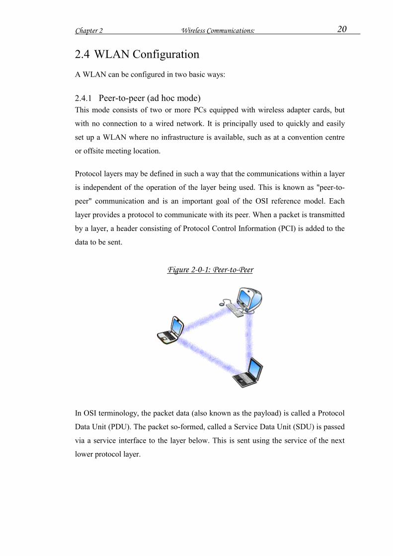
2.4.1 Peer-to-peer (ad hoc mode) This mode consists of two or more PCs equipped with wireless adapter cards, but
with no connection to a wired network. It is principally used to quickly and easily
set up a WLAN where no infrastructure is available, such as at a convention centre
or offsite meeting location.
Protocol layers may be defined in such a way that the communications within a layer
is independent of the operation of the layer being used. This is known as "peer-to-
peer" communication and is an important goal of the OSI reference model. Each
layer provides a protocol to communicate with its peer. When a packet is transmitted
by a layer, a header consisting of Protocol Control Information (PCI) is added to the
data to be sent.
Figure 2-0-1: Peer-to-Peer
In OSI terminology, the packet data (also known as the payload) is called a Protocol
Data Unit (PDU). The packet so-formed, called a Service Data Unit (SDU) is passed
via a service interface to the layer below. This is sent using the service of the next
lower protocol layer.

Chapter 2 Wireless Communications: 21
2.4.2 Client/server (infrastructure networking) A wireless network can also use an access point, or base station. In this type of
network the access point acts like a hub, providing connectivity for the wireless
computers. It can connect (or "bridge") the wireless LAN to a wired LAN, allowing
wireless computer access to LAN resources, such as file servers or existing Internet
Connectivity.
There are two types of access points:
�� Dedicated hardware access points (HAP) such as Lucent's WaveLAN,
Apple's Airport Base Station or WebGear's AviatorPRO. Hardware access
points offer comprehensive support of most wireless features with some
basic requirements carefully.
�� Software Access Points which run on a computer equipped with a wireless
network interface card as used in an ad-hoc or peer-to-peer wireless network.
Several programs are software routers that can be used as a basic Software
Access Point, and include features not commonly found in hardware
solutions, such as Direct PPPoE support and extensive configuration
flexibility. These may not however, offer the full range of wireless features
defined in the 802.11 standard. (Pahlavan, K. 1995)
Figure 2-0-2: Software Access Point
With appropriate networking software support, users on the wireless LAN can share
files and printers located on the wired LAN and vice versa.

Chapter 2 Wireless Communications: 22
2.4.3 Selection The WLAN Configuration used in the Wireless communication for the HSV project
was Peer-to-Peer. The network is only connecting two computers; therefore it would
be best to just communicate point to point. However, if we have more Utes to
control and communicate with at the same time it will also be possible to use the
peer-to-peer system.
2.5 Aim for the Wireless Communication The HSV Ute is controlled using the onboard computer; therefore, the Ute never had
the chance to be fully automated without anyone accessing the onboard computer by
physically being located inside the Ute for safety and control reasons. Using wireless
network communication, we will be able to access all the Ute sensors and control all
the actuators without directly using the onboard computer which processes the
automation algorithms. The wireless communication software will read all the
sensors data and control all the actuators. To do that we have to run two softwares at
the same time:
1. The first one will be running from the Ute’s onboard computer using
Hyperkernel and accessing the shared memory to read all the sensors data.
2. The second one will be running from the operator’s computer which sends
commands to the onboard computer and asks for information or gives
orders.

Chapter 3 Hardware 23
Chapter 3
3 Hardware
3.1 Structure
The wireless communication implementation for networking is exactly the same as the wired networking. However instead of using wire for linkage, we use some wireless hardware for the implementation. First of all, if we want to link two computers together we have to make a wireless connection between them. Each one needs to be connected to a wireless Ethernet card; either by just plugging the card into the laptop slot if it is available, or by using an extension box where it links the wireless card with the Ethernet network card of the computer. In the HSV project, the operator’s computer uses the wireless card by plugging it into the laptop slot, where the Ute computer uses an extension to connect its Ethernet card to the wireless card. For better range and more reliable connection each card is supported by an external antenna.
Figure 3-0-1: Wireless Communication Hardware
Chapter 3 Hardware 24
3.2 Antennas Antennas direct Radio Frequency (RF) power into a coverage area. Antennas are
available which produce differing coverage patterns. The correct antenna for a site is
chosen by determining the antenna that provides the coverage pattern best matched
to the site coverage requirements. Knowing the environment can help to determine
the right antenna and placement.
There are basically two types of antennas:
�� Omni-directional antennas have a 360-degree coverage pattern on a
horizontal plane. The coverage pattern is torus-shaped (like a doughnut).
These antennas are ideal for square or somewhat square areas.
�� Directional antennas concentrate the coverage pattern in one direction. This
produces an almost conical-shaped coverage pattern (like a flashlight). The
antenna directionality is specified by the angle of the beam width. Typical
beam width angles are from 90 degrees (somewhat directional), to as little as
20 degrees (very directional). The directed beam allows for a longer but
narrower coverage pattern, which is ideal for elongated areas, corners, and
outdoor point-to-point applications. (Liberti, J. 1999)
3.2.1 Gaining coverage range: The increase in coverage within the RF beam width is called the antenna gain, and is
measured in dB (decibels). Antenna gain improves the range of the signal for better
communications. For an unobstructed outdoor site, each 1dB increase in gain
approximately results in a range increase of 5%. Actual results vary depending on
the amount and type of obstructions at the site.
3.2.2 Positioning antennas: The proper positioning (orientation) of antennas at a site helps ensure the maximum
coverage area. Antennas should generally be mounted as high and as clear of
obstructions as practically possible. Best performance is attained when both
transmitting and receiving antennas are located at the same height and in direct line-
of-sight of each other.

Chapter 3 Hardware 25
3.3 Ute Antenna
The antenna chosen for the ‘Ute’ was 2.4 GHz 9dBi Omni-Directional for a circular coverage. A majority of the time, the ‘Ute’ is moving randomly towards different locations. Therefore, the Ute’s antenna cannot be angularly directed towards one side only. The antenna can be located anywhere in the ‘Ute’. It is recommended that the antenna be positioned on a high base not too close to the GPS’s (and the differential GPS) antenna. The antenna was mounted on the top bar of the Ute.
3.3.1 Specifications Frequency: 2400-2485 MHz
Gain: 9 dBi
Length/Weight: 27 inches, 2.0 lbs
OD Series Interface: N female connector
Mounting Kit: Mast mount kit included
Mounting Dimensions: Use mast up to 2" OD
Material: Polycarbonate with aluminium body, fiberglass
radome on OD12 with aluminium body
Nominal Impedance: 50 ohms
Max. Power (continuous): 100 watts
Vertical Beamwidth (-3 dB point): 9 dBi Model 14 degrees
Wind Loading (flat plate equiv.): 30-40 sq. inches
Rated Wind Velocity: 100+ mph
Antenna Diameter: 1", main mast
(Mobile Mark Antennas, 2002)
3.4 Operator Antenna The operator antenna is a 2.4 GHz, Rubber Duck/Portable Antenna, Half wave 2.5
dB gain styles with a flexible head. The 2.5 dB gain antenna also compensates for
typical system losses that occur at these frequencies. Physically the antenna is very
small which can be simply glued or connected to the side of the operator’s computer.
For a secure and reliable connection it can be mounted on a high base stick or
column.

Chapter 3 Hardware 26
3.4.1 Specifications Frequency: 2.4 - 2.485 GHz
Gain: 2.5 dBi max for 1/2 wave,
Bandwidth@2:1 VSWR: 85 MHz or better
Impedance: 50 Ohm nominal
Whip Length: 1/2 wave straight 4 inches
Maximum Power: 10 Watts
Whip Material: PSTN3 Series PVC jacket over dipole
(Mobile Mark Antennas, 2002)
3.5 Wireless Network Card There are a large number of suppliers of wireless LAN cards in the market.
Regardless of this, an ORiNOCO Silver PC card was used because it was available
at the centre. The card is however excellent with high standards.
3.5.1 Silver Label Cards Features The ORiNOCO Silver PC Cards supports the following wireless LAN features:
�� Automatic Transmit Rate Select mechanism in the transmit range of 11, 5.5, 2 and 1 Mbit/s.
�� Frequency Channel Selection (2.4 GHz). �� Roaming over multiple channels. �� Card Power Management. �� Wired Equivalent Privacy (WEP) data encryption, based on the 64 bit RC4
encryption algorithm as defined in the IEEE 802.11 standard on wireless LANs.
�� Plugs directly into laptop type-II PCMCIA slot �� Wi-Fi (IEEE 802.11b) certified interoperability �� Low power consumption �� Wide coverage range of up to 1,750ft/550m (Orinoco wireless card, 2002)
Chapter 3 Hardware 27
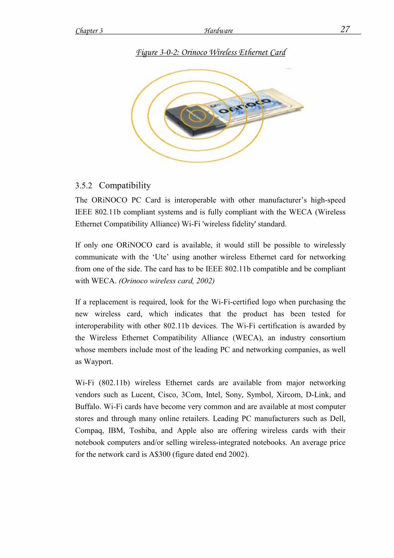
Figure 3-0-2: Orinoco Wireless Ethernet Card
3.5.2 Compatibility The ORiNOCO PC Card is interoperable with other manufacturer’s high-speed IEEE 802.11b compliant systems and is fully compliant with the WECA (Wireless Ethernet Compatibility Alliance) Wi-Fi 'wireless fidelity' standard. If only one ORiNOCO card is available, it would still be possible to wirelessly communicate with the ‘Ute’ using another wireless Ethernet card for networking from one of the side. The card has to be IEEE 802.11b compatible and be compliant with WECA. (Orinoco wireless card, 2002) If a replacement is required, look for the Wi-Fi-certified logo when purchasing the new wireless card, which indicates that the product has been tested for interoperability with other 802.11b devices. The Wi-Fi certification is awarded by the Wireless Ethernet Compatibility Alliance (WECA), an industry consortium whose members include most of the leading PC and networking companies, as well as Wayport. Wi-Fi (802.11b) wireless Ethernet cards are available from major networking vendors such as Lucent, Cisco, 3Com, Intel, Sony, Symbol, Xircom, D-Link, and Buffalo. Wi-Fi cards have become very common and are available at most computer stores and through many online retailers. Leading PC manufacturers such as Dell, Compaq, IBM, Toshiba, and Apple also are offering wireless cards with their notebook computers and/or selling wireless-integrated notebooks. An average price for the network card is A$300 (figure dated end 2002).

Chapter 3 Hardware 28
3.6 Ethernet Converter The WaveLAN Ethernet Converter (EC) device enables us to quickly transform
wired computing devices, such as (desktop) computers and/or printers into wireless
devices. Replacing 10Base-T Ethernet and/or RS-232 cables with WaveLAN
wireless technology allows us to:
�� Expand or relocate existing wired networks within minutes, without
additional costs for (re-)wiring and connecting computer terminals and/or
printers to the network.
�� Provide WaveLAN mobile connectivity to devices that once were “tied” onto
their network cables.
The WaveLAN IEEE product family is based upon a standard PC Card that can be
used in:
�� Portable computing devices equipped with a Type II PCMCIA card socket.
�� Desktop computers equipped with an ISA card bus (using an adapter).
�� Lucent Technologies WavePOINT-II access points.
(Orinoco wireless card, 2002)
Figure 3-3: Ethernet Converter Hardware
3.7 Data Protection and Security Wireless communications obviously provide potential security issues, as an intruder
would not need physical access to the traditional wired network in order to gain
access to data communications. However, 802.11 wireless communications cannot
be received --much less decoded-- by simple scanners, short wave receivers etc. This

Chapter 3 Hardware 29
has led to the common misconception that wireless communications cannot be
eavesdropped at all. However, eavesdropping is possible using specialist equipment.
To protect against any potential security issues, 802.11 wireless communications
have a function called WEP (Wired Equivalent Privacy), a form of encryption which
provides privacy comparable to that of a traditional wired network. If the wireless
network has information which should be secure, then WEP should be used,
ensuring the data is protected at traditional wired network levels.
Wired Equivalent Privacy (WEP) is a security protocol, specified in the IEEE
Wireless Fidelity (Wi-Fi) standard, 802.11b, which has been designed to provide a
wireless local area network (WLAN) with a level of security and privacy
comparable to what is usually expected of a wired LAN. A wired local area network
(LAN) is generally protected by physical security mechanisms (controlled access to
a building, for example) that are effective for a controlled physical environment, but
may be ineffective for WLANs because radio waves are not necessarily bound by
the walls containing the network. (Pahlavan, K. 1995)
WEP seeks to establish similar protection to that offered by the wired network's
physical security measures by encrypting data transmitted over the WLAN. Data
encryption protects the vulnerable wireless link between clients and access points;
once this measure has been taken, other typical LAN security mechanisms such as
password protection, end-to-end encryption, virtual private networks (VPNs), and
authentication can be put in place to ensure privacy.
It should also be noted that traditional Virtual Private Networking (VPN) techniques
will work over wireless networks in the same way as traditional wired networks.
3.8 Range Detection:
You can use the Client Manager icon on the Windows task bar to verify the link quality of your network connection. An overview of all possible icons is given in Table 3-1. When the Client Manager icon is not indicating excellent or good radio connection, check the recommended steps to follow in section 3.9 for range connection troubleshooting.

Chapter 3 Hardware 30
Table 3-1: Range Detection
Icon Colour Descriptions
Green Excellent radio connection
Green Good radio connection
Yellow Marginal radio connection.
Red
Poor radio connection:
The radio signal is very weak.
Red
No radio connection; Looking for initial
connection or moved out of range of the network
Blank Peer-to-Peer network connection is broken
The Client manager software also shows the percentage of communication data transfer rate for each side of the network. It divides the range into 4 main parts the 11mbits, 5.5mbits, 2mbits and 1mbits. The better the connection the more rates of 11mbits is used.
3.9 Range Troubleshooting:
The connection range should be around 550m in a reasonably clear environment using the previously selected antennas for a standard connection and safe data transfer. However, in a situation less than 550m where a connection has failed or is weak, check the following points:
�� Make sure the antenna cables are connected properly �� The best place to put the operator’s antenna is as close to the center of the
area that you want to cover. �� You'll probably do best if you orient your Wireless Router's antenna(s)
vertically. �� Keep antennas away from large metal objects like filing cabinets and away
from operating microwave ovens or 2.4GHz cordless phones. Also watch out for large containers of water... fish tanks or water heaters for example!

Chapter 3 Hardware 31
�� Most PC cards use an integrated antenna that is fairly directional. The horizontal orientation of these PC card antennas is not the best... it would work better if it were vertically oriented. Unfortunately no one has a PC card with a moveable antenna and it's not very practical to work with your laptop lying on its side!
�� If you're having trouble getting a strong signal with your laptop, try moving so that the PC card's antenna is pointing toward the Ute’s antenna. Also make sure your body isn't between the two antennas.
�� Avoid antenna placement close to an inside wall (unless inside is where you want to be!). Also, if you want to connect while you're inside, place the operator’s antenna near a window.
Chapter 4 Library Function 32
Chapter 4
4 Library Function
4.1 Background: The message-bus API msg_bus is a library to support inter-process and inter-system
communication using the socket interface. The library uses the datagram message
protocol (UDP) as provided by IP. This choice was made, rather than using TCP, for
performance reasons and because the underlying (Switched Fast Ethernet in hub-
spoke layout) medium is reliable by itself: full-duplex point-to-point communication
between nodes and collision detection with resending of lost packets. The library is
for C++ coding syntaxes.
4.2 Message Bus Functions: A distributed system consists of a number of systems (called nodes) where on every
node a number of processes (called tasks) can be running. The purpose of a message
bus is to enable these tasks to communicate for information exchange and for
synchronization purposes.
The reason for using a message bus for these exchanges is to avoid a large network
of point-to-point connections and to get modular system architecture. The aim is to
be able to communicate (message passing) between tasks on different nodes or
between tasks on the same node without causing any changes for other tasks in the
system.
The msg_bus library consists of a number of functions to be called by client, server
and peer-to-peer programs. By using these calls a fully distributed message passing
system can be realized in any of the supported operating systems.

Chapter 4 Library Function 33
The four main functions are:
�� msg_attach - initialise communication message bus
�� msg_detach - release connection with message bus
�� msg_send - send a message to another task and/or node
�� msg_receive - wait for a message to arrive and read it
The msg_bus library has a large number of functions that are not used in this thesis.
4.2.1 Attached: The msg_bus library function msg_attach is the first to be called by any process that
wishes to use msg_bus. It will use the node and task to create a socket and to setup a
global structure with common data. The function returns MSG_OK (0) when
attachment is successful or one of the error codes in case of socket is open, bind, or
set-errors.
node
The node name of the own system (actually the IP address) represented by a string in
the format of “xxx.xxx.xxx.xxx” (for example “155.69.31.90”).
task
The task name of the own system: This should be a string, representing an integer
(actually a port number) in the range of 1024 to 65535 (for example “5016”)
4.2.2 Detach: The msg_bus library function msg_detach should be called before quitting the
application that uses the msg_bus. It will close the socket. No parameters are
required.
long msg_detach( );
long msg_attach(char *node, char *task);

Chapter 4 Library Function 34
4.2.3 Sending: The msg_bus library function msg_send is used to send a message to another task.
The function will add an envelope with sender and receiver info. To be able to send,
the socket must attach first by using msg_attach(). The message ID and length will
(if necessary) be converted to network-byte order. For the contents of the data field
it is the responsibility of the application to do this. To be sure that it is received, the
back parameter has to be set to true. msg_send() will then wait for an
acknowledgment (of course using a timeout) before it returns. The function returns
MSG_OK (0) when the sending is successful, or one of the other error codes in case
of an error with sending, time-out or acknowledgment.
n
T
r
“
t
T
i
i
T
b
l
T
d
T
long msg_send( char *node, char *task, long id, long len, char *data, bool ck );
ode
he node name of the system (IP address) where the task resides. The node name is
epresented by a string in the format of “xxx.xxx.xxx.xxx” (for example
155.69.31.90”).
ask
he task name of the destination process: this should be a string, representing an
nteger (actually a port number) in the range of 1024 to 65535 (for example “5016”)
d
he identifier of the message to send (the ID of the structure of the message, needed
y the receiving task to extract the data).
en
he length, in bytes, of the following data block.
ata
he data block, this is a string.

Chapter 4 Library Function 35
ack
Boolean to set TRUE if the sender wants to wait for acknowledgement of receiving.
4.2.4 Receiving: The msg_bus library function msg_receive will get a message from a socket and
respond with message ID and data. A timeout value can be given to wait a maximum
number of seconds. When a timeout happens, the function will return with the error
code MSG_ERR_TIMEOUT(-30). If the timeout is set to -1 the function will wait
forever for an incoming message (this will be used in a setup where the receiving
task is linked to an incoming event to provide callback functionality). The function
returns MSG_OK (0) when receiving the message is successful or one of the error
codes in case of an error while receiving, time-out or acknowledgment.
When receiving a data structure, this structure can only be determined after the
message ID is known. We create a pointer to a structure right format and assign it to
the unstructured data field to access the data.
n
T
T
e ta
T
( id
T
a
th le
T
long msg_receive ( char *node, char *task, long *id, long *len, char *data, long timeout);
ode
he node name of the system (the IP address) where the sending process originates.
he node name is represented by a string in the format of “xxx.xxx.xxx.xxx” (for
xample “155.69.31.90”).
sk
he task name of the sending process: this should be a string, representing an integer
actually a port number) in the range of 1024 to 65535 (for example “5016”)
he identifier of the received message. The ID is used by the sending task upon
greement with the receiving task to define the structure of the message, needed by
e receiving task to extract the data.
n
he length, in bytes, of the following data block

Chapter 4 Library Function 36
data
The data block, which is a string.
timeout
The number of milli-seconds to wait for an incoming message. When the timeout is
zero the function will only return with data which was present in the queue. When
negative, this function will block and wait until a message arrives.
4.3 Urgent Messages The library can distinguish between normal messages and urgent messages. For
every task that uses a communication channel also an urgent channel can be opened.
If the normal communication channel is blocked, the urgent channel still can be used
The msg_bus library function msg_attach_urgent is similar to msg_attach however a
different socket is opened to provide a separate channel for urgent messages. This
urgent channel is needed because for urgent messages it is unacceptable to get
queued or even get lost because of buffer overflow.
The function is to be called by any process that wishes to use the urgent-channel
facilities of the msg_bus. It should be called at initialisation together with
msg_attach() The function returns MSG_OK (0) when attachement successful or
one of the error codes in case of socket open, bind, or set-errors.
The same th
The parame
long msg_attach_urgent( char *node, char *task);
ing will apply to sending messages, receiving messages and detaching.
ters are the same and look like the following:

Chapter 4 Library Function 37
Icu
long msg_send_urgent( char *node, char *task, long id, long len, char *data, bool ack );
long msg_receive_urgent ( char *node, char *task, long *id, long
*len, char *data, long timeout ); msg_detach_urgent( );
n the project the urgent messages weren’t used because basically the ommunication messages were quite simple and on at the time. None of them were rgent.

Chapter 5 Software Development 38
Chapter 5
5 Software Development 5.1 Introduction At this stage of the thesis the hardware setup has been finalized and the networking
communication library was understood. Therefore the next stage is going to be the
software development. Software development had a general architecture that was
divided into five main stages: Requirement, design, coding, testing and maintenance.
The following graph shows the procedure taken into the development of the
software. After finalising some specific parts however, there was sometimes a need
to take it into consideration again because the architecture has a strong linkage with
the individual parts.
Figure 5-1: Software Development Stages
Requirements
Design
Coding
Testing
Maintenance
Chapter 5 Software Development 39
5.2 Requirements The aim of the thesis is to design and build a wireless communication package that
is used to network the Ute’s onboard computer with the operator’s computer
wirelessly where commands, messages and sensor data can be transferred from one
computer to the other.
The final specification was that the software has to make a networking linkage
between the two computers where the operator can send some commands to the
Ute’s computer asking to send him some specific sensor data, or all the sensors data,
and the control constants for the actuators such as the starting point, Kp, Ki, Kd… the
data has to be saved on the operator computer, each sensor or each division in its
own txt file. Each file has to start with some specification about what the data is, the
starting date and time for the data collection and finish with the date and time of
ending of the data collection.
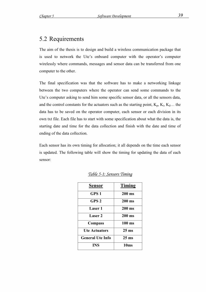
Each sensor has its own timing for allocation; it all depends on the time each sensor
is updated. The following table will show the timing for updating the data of each
sensor:
Table 5-1: Sensors Timing
Sensor Timing GPS 1 200 ms
GPS 2 200 ms
Laser 1 200 ms
Laser 2 200 ms
Compass 100 ms
Ute Actuators 25 ms
General Ute Info 25 ms
INS 10ms

Chapter 5 Software Development 40
The selection of a combination of 2, 3 or more sensors would also be recommended,
because sometimes we only need a combination of just 2 or 3 sensors for navigation
or control. The rest would be useless for us, which is why it would be possible to
record the specified sensors using only some Dos interface.
5.3 Design As was discussed earlier, we had to design two individual softwares: one for the Ute
and another one for the operator. The Ute program was quite simple and straight to
the point whereas the operator program was a bit more complicated.
The main software architecture is summarised by the following graph. The first thing to do is to create a link between the two computers by attaching the individual IP addresses together. The operator will then send a message to the Ute where it will ask for some specific data (usually sensors data). The Ute software will read the data from the shared memory (Hyperkernel shared memory) and will send it to the operator’s computer. The operator software will finally write the data into a text file. The software will be terminated when the operator desires it and the two programs will then break the link between them. In the following part, the design for each individual software is discussed in full detail.
Figure 5-2: Main Software Architecture
Sending Data
Write to TXT Files
Read Shared
Memory
Message with ID
Wireless Network
Connection
Operator Software
Ute’s Software

Chapter 5 Software Development 41
5.3.1 The Ute’s Software The Ute’s software is pretty straight forward. The aim is to get the message search
for the data and send it to get the new one. This procedure should then repeat again
and again. If it doesn’t receive a message it will just wait forever.
The first thing is to get connected to the Hyperkernel shared memory where it will
have access to all the sensors. It will read all the sensors structure at real time.
Therefore, all the sensors data are updated each time the Hyperkernel updates the
sensors. Not all the sensors structure is requested however all the structure will be
sent and what is required will be saved.
The next step is detecting the IP address then attaching to the other software. A
networking link will be created. Then it will wait forever until it receives a message.
Each message received will mainly have no data in it (however we can send any data
or structure we want) it will only have a message ID. Each message ID number is a
request for some specific data. At this stage we will have a switching function that
contains nine different cases.
The first case is just a heart beat signal; in other words it is just a check up if the
connection is alive. The other eight cases are for the eight different set of sensors
structure. Each one is for individual sensors such as GPS, Laser, INS and Compass.
However, the encoder and actuator control values are only sent in two different
structures; one contains all the actuators positions and the wheel encoder and the
other one contains all the controllers’ settings.
Each sensor structure is sent on its own, one at a time. The speed of sending the data
is very fast, much smaller than the time each sensor is updated. Therefore, the
software can send all the sensors values before being delayed by any of them. After
sending all the data required, it will detach whenever the software is terminated by
receiving a message ID 0 for detaching.
The following figure shows the architecture step by step for the Ute’s software in
full detail.

Chapter 5 Software Development 42
Figure 5-3: Ute's Software Architecture
Attaching to Network
Ready to read the message
Switch (msg_id)
If 1
If 2
If 5
If 4
If 3
Alive message
Read GPS1 & send it
Read GPS2 & send it
Read Laser1 & send it
Read Laser2 & send it
If 6Read Compass & send it
If 7
If 0 Detaching from Network
While (True)
If 9 Read Ute Info & send it
Read Actuators & send it If 8
Read INS & send it
Chapter 5 Software Development 43
5.3.2 The Operator’s Software The operator program is where the decision has to be taken by the operator to decide
what kind of data is requested. In this part the operator has full control on the actions
of the Network communication.
The first part is attaching to the Ute’s computer that has to be running on the other
side and waiting for connection. To attach, the software will look for the computer
IP address and then make the connection using the msg_attach function.
The next part is detecting the date and the time the connection is made. Then it will
create eight different text files, one for each sensor. After creating the files it will
write the type of data saved in the file with the date and the time on the first line.
The next line would be the definition of each column of data. All of them will start
with the timestamp and then the sensors data such as latitude, longitude, mode,
satellite and so on (that was some of the GPS values)…
The following part is a section into a while loop always True till the operator wishes
to exit the program. At the beginning the operator will choose what kind of data they
want to request from the Ute. There are four main reasons:
1. Check if the connection is alive.
2. Exit the program and detach from the network.
3. Receive all the sensors data and save them into the text files.
4. Choose only specific sensors - one, two, three or more. In this stage, the
operator has to allocate the sensors one by one.
If the selection is incorrect, the operator can stop anything that is running and go
back to the selection. After running a test and saving some data at the same time
another selection of sensors can be made and new data will be saved. After the
operator is satisfied and he wishes to disconnect and terminate the program, he can
interrupt the process by choosing to exit, and the software will disconnect from the
network.
The following chart will show the software architecture of the operator’s software in
full details of operation. Each part might be made of other small parts that would be
included in it.

Chapter 5 Software Development 44
Figure 5-4: Operator's Software Architecture
&
&
&
Attaching to Network
Read Date & Time
Opening Text Files for Sensors
Select Data Required
While (True)
Check if Connection Alive
Send to FGPS1.txt
Ask for GPS1 Receive it200ms If Required
Or Send to
FGPS2.txt Ask for GPS2
Receive it200ms If Required
Send to FLaser1.txt
Ask for Laser1 & Receive it200ms If Required
Send to FLaser2.txt
Ask for Laser2 & Receive it200ms If Required
Send to FCompass.txt
Ask Compass Receive it100ms If Required
Send to FInfo.txt If Required
Send to FActuators.txt If Required
Send to FINS.txt If Required
Ask for INS & send it10ms
Ask Actuators & Receive it25ms
Read Actuators & Receive it25ms
Detach from Network
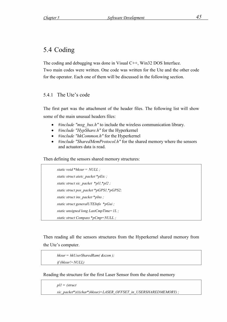
Chapter 5 Software Development 45
5.4 Coding
The coding and debugging was done in Visual C++, Win32 DOS Interface. Two main codes were written. One code was written for the Ute and the other code for the operator. Each one of them will be discussed in the following section.
5.4.1 The Ute’s code The first part was the attachment of the header files. The following list will show
some of the main unusual headers files:
�� #include "msg_bus.h" to include the wireless communication library. �� #include "HypShare.h" for the Hyperkernel �� #include "hkCommon.h" for the Hyperkernel �� #include "SharedMemProtocol.h" for the shared memory where the sensors
and actuators data is read. Then defining the sensors shared memory structures:
static void *hksur = NULL ;
static struct aietc_packet *pEtc ;
static struct sic_packet *pl1,*pl2 ;
static struct pos_packet *pGPS1,*pGPS2;
static struct ins_packet *pIns ;
static struct generalUTEInfo *pGui ;
static unsigned long LastCmpTime=1L ;
static struct Compass *pCmp=NULL ;
Then reading all the sensors structures from the Hyperkernel shared memory from
the Ute’s computer.
hksur = hkUserSharedRam( &szsm );
if (hksur!=NULL)
Reading the structure for the first Laser Sensor from the shared memory
pl1 = (struct
sic_packet*)(((char*)hksur)+LASER_OFFSET_in_USERSHAREDMEMORY) ;

Chapter 5 Software Development 46
Reading the structure for the second Laser Sensor from the shared memory
pl2 = pl1+1 ;
Reading the structure for the first GPS Sensor from the shared memory
pGPS1 = (struct
pos_packet*)(((char*)hksur)+GPS1_OFFSET_in_USERSHAREDMEMORY) ;
Reading the structure for the second GPS Sensor from the shared memory
pGPS2 = pGPS1+1 ;
Reading the structure for the Ute general Sensor such as encoders from the shared
memory
pEtc = (struct
aietc_packet*)(((char*)hksur)+ETC1_OFFSET_in_USERSHAREDMEMORY) ;
Reading the structure for the INS Sensor from the shared memory
pIns = (struct ins_packet *)
(((char*)hksur)+INS_OFFSET_in_USERSHAREDMEMORY) ;
Reading the structure for the Compass Sensor from the shared memory
pCmp = (struct Compass*)
(((char*)hksur)+COMPASS_OFFSET_in_USERSHAREDMEMORY) ;
Reading the structure for the General Ute info such as setting points for controllers
from the shared memory
pGui = (struct generalUTEInfo *)((char*)hksur
+ETC2_OFFSET_in_USERSHAREDMEMORY) ;
The next part would be detecting the IP address of the Ute’s computer for future
connection to the network.
//Cheking the IP Adresses
WORD wVersionRequested;
WSADATA wsaData;
char name[255];

Chapter 5 Software Development 47
PHOSTENT hostinfo;
wVersionRequested = MAKEWORD( 2, 0 );
if ( WSAStartup( wVersionRequested, &wsaData ) == 0 )
{
if( gethostname ( name, sizeof(name)) == 0)
{
if((hostinfo = gethostbyname(name)) != NULL)
{
own_node = inet_ntoa (*(struct in_addr *)*hostinfo->h_addr_list);
printf("\n the IP is %s \n \n",own_node);
}
}
WSACleanup( );
}
After detecting the IP address the wireless networking connection will be made
using the msg_attach function from the “Msg_bus” Library. The “own_node” is the
IP address and the “5220” is a randomly chosen port number.
/* connect to the message bus */
if ((rc = msg_attach (own_node, "5220")) != MSG_OK)
msg_error (rc);
The next stage is a while loop that is always true.
After that the program will use the msg_receive function where it wait for a message
form the operator’s computer and aiming to read it’s msg_id and then decide which
stage to go to using the switching function.
while(1){
rc = msg_receive (snd_node, snd_task, &msg_id, &msg_len, msg_data,-1);
if(rc!=MSG_OK)
msg_error (rc);
printf("id is %d\n", msg_id);
switch(msg_id)
{

Chapter 5 Software Development 48
Case one is when the operator is just checking if eth connection is alive. Therefore,
the message received will contain nothing except 1 as ID. Case will return an empty
message again with ID equal to 1.
case 1:
{
if ((rc = msg_send("snd_node", "5110", 1, 0, NULL, FALSE)) != MSG_OK)
msg_error (rc);
break;
}
The rest of the cases are sending the sensors data whenever they are requested. Only
the first GPS case is outlined and explained. The case ID for the GPS is 2. The main
task for this case is sending the GPS2 data structure.
case 2: // Send GPS1
{
rc = msg_send (own_node,"5110", msg_id, sizeof(struct pos_packet),(char*) pGPS1, -1);
if(rc!=MSG_OK)
msg_error (rc);
break;
Case Zero is where the user is asking to terminate the program and break the
wireless network connection.
case 0:
{
if ((rc = msg_detach ()) != MSG_OK)
msg_error (rc);
5.4.2 The Operator’s Software The first part was the attachment of the header files. The following list will show
some of the main unusual headers files:
�� #include <time.h> for detecting the date and the time �� #include "msg_bus.h" to include the wireless communication library. �� #include "SharedMemProtocol.h" for the shared memory where the sensors
and actuators data is read.

Chapter 5 Software Development 49
The next part would be detecting the IP address of the Operator’s computer for
future connection to the network.
//Cheking the IP Adresses
WORD wVersionRequested;
WSADATA wsaData;
char name[255];
PHOSTENT hostinfo;
wVersionRequested = MAKEWORD( 2, 0 );
if ( WSAStartup( wVersionRequested, &wsaData ) == 0 )
{
if( gethostname ( name, sizeof(name)) == 0)
{
if((hostinfo = gethostbyname(name)) != NULL)
{
ip = inet_ntoa (*(struct in_addr *)*hostinfo->h_addr_list);
printf("\n the IP is %s \n \n",ip);
}
}
WSACleanup( );
}
After detecting the IP address the wireless networking connection will be made
using the msg_attach function from the “Msg_bus” Library. The “own_node” is the
IP address and the “5110” is a randomly chosen port number.
/* connect to the message bus */
if ((rc = msg_attach (ip, "5110")) != MSG_OK)
msg_error (rc);
The next step is reading the date and eth time from the computer. The date and the
time will be read from the windows operating system.
// Time
time(&bintime);
curtime=localtime(&bintime);

Chapter 5 Software Development 50
The next step is opening eight different files each one for a specific sensor. The files
are ASCII format. The first line in the will be the definition of what the file contains
then what date and time was created. After that, the value of each column will be
defined. It might not be aligned with the column but it will be clear enough to
identify the data. The following example is just for the GPS1 data. The rest of eth
sensors files are created using the same procedures.
// Oppening GPS1
if( (FGPS1 = fopen( "FGPS1.txt", "w" )) == NULL )
printf( "The file was not opened\n" );
fprintf(FGPS1, "The File Contains the First GPS Data on: %s",
ctime(&bintime));
fprintf(FGPS1, "timestamp, latitude, longitude, altitude, ttcourse, speedog,
vspeed, sigmaLati, sigmaLongi, sigmaAlti, mode, satellites");
At this stage, the operator will be able to decide one of four main option: 1. The letter " e " to exit 2. The letter " a " for all the sensors to be retrieved and saved 3. The letter " p " to check if the connection is alive 4. The letter " s " to select some specific sensors and/or actuators data
while(msg_id!=0)
{ if (id_imput!="0" | id_imput!="1" | id_imput!="2" | id_imput!=3 )
{
printf( "\n Please choose one of the following options: \n" );
printf( "\n -> the letter " 0 " to exit \n" );
printf( "\n -> the letter " 2 " for all the sensors to be retrieved and saved\n" );
printf( "\n -> the letter " 1 " to check if the connection is alive\n" );
printf( "\n -> the letter " 3 " to select some specific sensors and/or actuators data\n" );
gets( id_input);
}
If the letter “0” is selected, the operator is wishing to exit. Therefore the message
sent to the Ute will have an ID of zero that request network disconnection. So the
two computers will detach from the network and the communication link will brake.
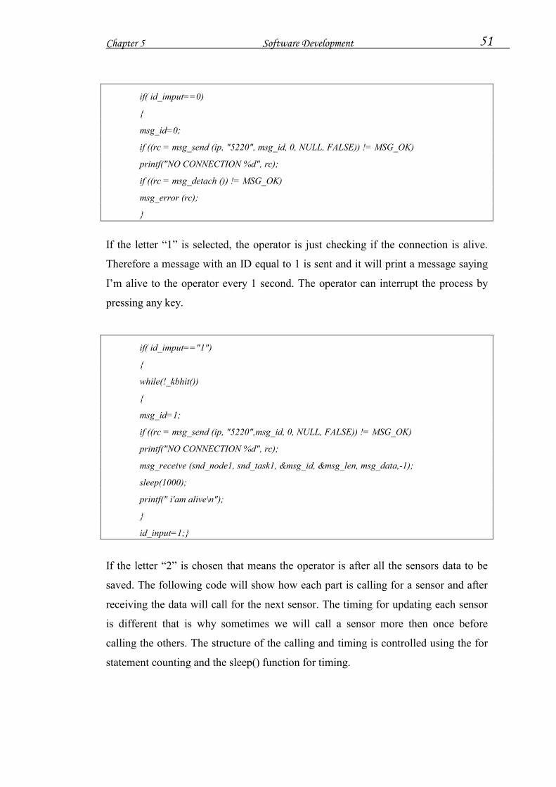
Chapter 5 Software Development 51
if( id_imput==0)
{
msg_id=0;
if ((rc = msg_send (ip, "5220", msg_id, 0, NULL, FALSE)) != MSG_OK)
printf("NO CONNECTION %d", rc);
if ((rc = msg_detach ()) != MSG_OK)
msg_error (rc);
}
If the letter “1” is selected, the operator is just checking if the connection is alive.
Therefore a message with an ID equal to 1 is sent and it will print a message saying
I’m alive to the operator every 1 second. The operator can interrupt the process by
pressing any key.
if( id_imput=="1")
{
while(!_kbhit())
{
msg_id=1;
if ((rc = msg_send (ip, "5220",msg_id, 0, NULL, FALSE)) != MSG_OK)
printf("NO CONNECTION %d", rc);
msg_receive (snd_node1, snd_task1, &msg_id, &msg_len, msg_data,-1);
sleep(1000);
printf(" i'am alive\n");
}
id_input=1;}
If the letter “2” is chosen that means the operator is after all the sensors data to be
saved. The following code will show how each part is calling for a sensor and after
receiving the data will call for the next sensor. The timing for updating each sensor
is different that is why sometimes we will call a sensor more then once before
calling the others. The structure of the calling and timing is controlled using the for
statement counting and the sleep() function for timing.

Chapter 5 Software Development 52
if( id_imput==2)
{msg_id=2;
if ((rc = msg_send (ip, "5220", msg_id, 0, NULL, FALSE)) != MSG_OK)
printf("NO CONNECTION %d", rc);
while(!_kbhit())
{for(int d=0; d<1; d++)
{
// GPS 1
msg_receive (snd_node1, snd_task1, &msg_id, &msg_len, msg_data,-1);
GPS1=*(pos_packet *)msg_data;
fprintf(FGPS1,"%d %d %d %d %d %d %d %d %d %d %d %d \n",GPS1.timestamp,
GPS1.latitude,GPS1.longitude,GPS1.altitude,GPS1.ttcourse,GPS1.speedog,GPS1.vspeed,GPS1.sigm
aLati,GPS1.sigmaLongi,GPS1.sigmaAlti,GPS1.mode,GPS1.satellites);
msg_send (ip, "5220", 3, 0, NULL, FALSE);
// GPS 2
msg_receive (snd_node1, snd_task1, &msg_id, &msg_len, msg_data,-1);
GPS2=*(pos_packet *)msg_data;
fprintf(FGPS2,"%d %d %d %d %d %d %d %d %d %d %d %d \n",
GPS2.latitude,GPS2.longitude,GPS2.altitude,GPS2.ttcourse,GPS2.speedog,GPS2.vspeed,GPS2.sigm
aLati,GPS2.sigmaLongi,GPS2.sigmaAlti,GPS2.mode,GPS2.satellites,GPS2.timestamp);
msg_send (ip, "5220", 4, 0, NULL, FALSE);
// Laser 1
msg_receive (snd_node1, snd_task1, &msg_id, &msg_len, msg_data,-1);
l1=*(sic_packet *)msg_data;
for (j=0;j<361;j++)
{l1.range[j] ;
fprintf(FLaser1,"%d ",l1.range[j]);}
fprintf(FLaser1,"\n");
msg_send (ip, "5220", 5, 0, NULL, FALSE);
// Laser 2
msg_receive (snd_node1, snd_task1, &msg_id, &msg_len, msg_data,-1);
l2=*(sic_packet *)msg_data;
for (j=0;j<361;j++)
{l2.range[j] ;
fprintf(FLaser2,"%d ",l2.range[j]);}

Chapter 5 Software Development 53
fprintf(FLaser2,"\n");
msg_send (ip, "5220", 6, 0, NULL, FALSE);
for(int c=0; c<2; c++)
{
// Compass
msg_receive (snd_node1, snd_task1, &msg_id, &msg_len, msg_data,-1);
Cmp=*(Compass *)msg_data;
fprintf(FCompass,"%d %d %d\n",Cmp.Heading,Cmp.Pitch,Cmp.Roll);
msg_send (ip, "5220", 8, 0, NULL, FALSE);
for(int b=0; b<5; b++)
{
// Actuators
msg_receive (snd_node1, snd_task1, &msg_id, &msg_len, msg_data,-1);
Ins=*(ins_packet *)msg_data;
fprintf(FActuators,"%d %d %d %d %d\n", Etc.Counts ,Etc.Accelerator ,Etc.Steering, Etc.Brake
,Etc.timestamp);
msg_send (ip, "5220", 9, 0, NULL, FALSE);
// Send Ute Info
msg_receive (snd_node1, snd_task1, &msg_id, &msg_len, msg_data,-1);
Gui=*(generalUTEInfo *)msg_data;
fprintf(FActuators,"%d %d %d %d %d %d %d %d %d %d\n", Gui.PID_A.Kp, Gui.PID_A.Ki,
Gui.PID_A.Kd, Gui.PID_A.SeMin ,Gui.PID_A.SeMax, Gui.PID_A.yMin, Gui.PID_A.yMax,
Gui.PID_A.spoint,Gui.SteeringControlMode,Gui.manual_steering);
msg_send (ip, "5220", 7, 0, NULL, FALSE);
for(int a=0; a<2; a++)
{
// INS
msg_receive (snd_node1, snd_task1, &msg_id, &msg_len, msg_data,-1);
Ins=*(ins_packet *)msg_data;
fprintf(FINS,"%d %d %d %d %d %d %d %d\n" ,Ins.bank, Ins.elev, Ins.ax,Ins.ay, Ins.az, Ins.gx,
Ins.gy, Ins.gz);
msg_send (ip, "5220", 2, 0, NULL, FALSE);
printf("Count %d \n",a);
Sleep(10);
} } } } }
printf( "\n Please Enter the ID Number\n" );
gets( id_input);}

Chapter 5 Software Development 54
If the operator chooses the letter “3” then a series of selection he/she will have to go
through. The program will ask him for every single set of sensors data if it is
required to be read and saved. Then whenever the sensor is not selected saving it to
the txt will be ignored. The structure of that part will be exactly the same as the
previous part with more if statement for selection.
5.5 Testing & Maintenance After debugging the codes and getting rid of all the main debugging errors and
warnings, some code weaknesses were discovered. I was successful in fixing some
of them but others were difficult and required an extensive amount of time. The
following part will discuss some of the code weaknesses:
Because the softwares are running at real time and the Ute’s program is using the
Hyperkernel shared memory, we have to run the Hyperkernel software to read the
sensors at real time and save them in the shared memory. Therefore, the Ute’s
software will be accessing and sending fresh sensor’s data to the operator through
the wireless communication network. The implementation can be done without
running the Hyperkernel if we join the two softwares together with the Hyperkernel
and the communication. However this would take a lot of unwanted effort.
As has been discussed before, we are able to select between sensors data to save it in
text files. However if we choose to save the GPS1 first, followed by the laser and
back to the GPS1 data again, it will continue wherever it finished saving from the
previous part of the GPS1 with a new set of timestamps. However if we exit the
software, and run it again by selecting the GPS1, it will overwrite the existing GPS1
data. It is recommended to save the files in a different directory each time a test is
finished. A solution to this would be letting the program create a new directory each
time we run it where its name is related to the date and time, and record the data in
it.

Chapter 5 Software Development 55
Another weakness that was discovered is that if we make the operator’s program
print the data required on the screen it will slow the processor and makes reading
data process slower which can lead to a delay in sensor’s update. Therefore, printing
the data on the screen was cancelled to prevent any delay. All the data will only be
saved on the text files.
The data text output was first created as ASCII files. It was recommended to save
larger data files as binary. However, space does not really matter when using the
operator’s computer. Having a hard disk of at least 10Gbyte would be more than
enough for the sensors data for hours of testing. However, if binary type files are
required it would be an easy option to implement by giving the option to save before
creating the file. I would prefer to use ASCII because it is easier to understand and
easier to use for graphing or filtering without the need for any code or library for
translation.
With the operator’s software, the user will have a choice of selections regarding data
transfer and saving at the beginning of the program. At this stage a wrong input
would lead to a wrong decision implementation. Therefore, an error detection
procedure was designed to prevent wrong input commands that would lead to wrong
code implementation and processing.

Chapter 6 Safety 56
Chapter 6
6 Safety
6.1 Aims This chapter is written for two main reasons
�� To reduce the incidence of accidents & injuries (and associated pain,
suffering, costs and lost time) within the ACFR centre and especially within
the HSV Project
�� To comply with the NSW Occupational Health and Safety Regulation 1991.
6.2 Occupational Health and Safety Policy The Australian Centre for Field Robotic is committed to providing a healthy and
safe workplace and to eliminating conditions and incidents which could result in
personal injury or ill health. The ACFR requires its activities to conform to relevant
state and federal legislation and good, established practices including Australian
Standards.
The Centre recognises that success depends on the commitment and cooperation of
staff and students. The ACFR expects staff and students to comply with its
occupational health and safety policies, procedures and guidelines, and to conduct
themselves in a safe manner, not placing themselves or others at risk. Members of
staff are responsible for the health and safety of staff and students working under
their direction. The ACFR is also responsible for providing a safe and healthy
environment for its visitors and members of the public who come onto University
premises or are affected by the University's activities.
Chapter 6 Safety 57
6.3 HSV Project Safety The ACFR centre at the University of Sydney never had major accidents which led
to any injury. The zero number of injuries / accidents is a result of the strict safety
rules that the centre obliges the staff, students, researchers and visitors to follow
when working (even if just watching) on any project. The HSV project is a project
that involves a lot of risky activities while working on it, especially during testing.
One of the project aims is to design a fully automated vehicle that is able to scan,
navigate at a high speed and create a map of the environment. At the moment the
‘Ute’ can only do very specific tasks regarding automation, however, it is still very
dangerous to leave the onboard ‘Ute’ computer with full control of the actuators.
While it is capable of doing proper and safe tasks, it remains a risk. Therefore,
operators have to be located inside the vehicle at anytime when the car engine is
ON.
6.4 Safety Procedures When someone is working within the HSV project, their safety and the safety of the
people around them has to be taken into consideration. He/she shall not undertake
any risky activities. Therefore, if the person is unsure about the risk level of the
activity, he/she shall consult the supervisor or any of the experienced team members
of the HSV project.
When working on the ‘Ute’, installing hardware, testing components, driving the
‘Ute’, doing a run test or any other activity involving the ‘Ute’ he/she shall adhere to
the following procedures:
Test procedure:
�� Any test on the ‘Ute’ has to be approved by the supervisor.
�� The driver should have a full driver’s licence authorized by RTA Australia,
or any equivalent international driver’s licence approved by the RTA
�� The diver should fill in a form requested by the ACFR management only
once before driving any University vehicles.
�� Whenever a test is required, at least 2 people have to be on site (being on

Chapter 6 Safety 58
your own is not enough).
�� The driver shall never leave the drivers seat whenever the ‘Ute’ is ON.
�� In the Automatic status the Ute’s computer should not be fully trusted to be
in full control. Driver has to be ready for any surprises.
�� The testing speed should not exceed 20 Km/h.
�� The driver and the passenger should always wear their seat belts.
�� Be careful when the wireless communication antenna is mounted not to go
into car parks or under roofs that are less then 2.4 meters high.
�� After any testing, turn off all the sensors and actuators.
�� Shut down the onboard computer.
�� Be sure to place the gear on “P”, handbrake on and give keys back to the
supervisor.
If an emergency occurs in the automated status, the following steps should be
adhered to (one or more actions can be handled at the same time):
�� Apply the foot brake to the maximum.
�� Turn off the car.
�� Switch the mode from automated to manual by pressing the auto/man
switch located on the dashboard next to the Hazards switch to disengage
the electromagnetic clutch that control the steering wheel.
�� Apply the hand brake.
�� Turn off the power to the actuators.
�� If any accident or injury occurs, report it as soon as possible. (For more
details about this section read the next part: “Procedures when accidents
happen”).
6.5 Procedures: When Accidents Happen These procedures have to be followed whenever any accidents occur within the
ACFR building, University properties and/or while working on the HSV project at
anytime or anywhere.

Chapter 6 Safety 59
1. Importance of Reporting
Reporting of accidents is essential for the identification of hazards in the workplace.
Remedial action can then be taken to address the identified hazards and prevent any
recurrence of the incident. Reporting is to be made by staff, students or visitors who
are injured or become ill in connection with their work when visiting or working at
the University. Incidents with potential for injury or damage (near misses) should
also be reported. The accident report also acts as a record for future reference should
there be any subsequent complication for example, delayed health effects that may
require the report as a factual base.
2. Minor Injuries
Minor injuries which require no treatment or minor first aid treatment only, should
also be reported to prevent it from happening at any other time with more serious
effects.
3. ACCIDENT INVESTIGATION
Reported accidents and incidents should be promptly investigated by the immediate
supervisor of the injured or ill person, or by the person in charge of the area where
the incident occurred. The investigation should identify the causes of the accident
and any hazards that need to be controlled. Supervisors should then take action to
control the hazards which have been identified.
6.6 WaveLAN Health Safety WaveLAN, like other radio devices, emits radio frequency electromagnetic energy.
The level of energy emitted by WaveLAN devices however is far much less than the
electromagnetic energy emitted by wireless devices like for example mobile phones.
Because WaveLAN operates within the guidelines found in radio frequency safety
standards and recommendations, it is believed that WaveLAN is safe for use by
consumers. These standards and recommendations reflect the consensus of the
scientific community and result from deliberations of panels and committees of
scientists who continually review and interpret the extensive research literature.
In some situations or environments, the use of WaveLAN may be restricted by the

Chapter 6 Safety 60
proprietor of the building or responsible representatives of the organization. These
situations may for example include:
�� Using the WaveLAN equipment on board airplanes, or
�� In any other environment where the risk of interference to other devices or
services is perceived or identified as harmful.
If you are uncertain of the policy that applies to the use of wireless devices in a
specific organization or environment (e.g. airports), you are encouraged to ask for
authorization to use the WaveLAN device prior to turning on the equipment.
6.7 Conclusion In summary, the above is just a basic outline of what staff, students or visitors
should take into consideration in relation to safety procedures. Safety in the
workplace results in mental and physical well-being, as well as cost and time-saving
efficiencies. Adhering to safety procedures also ensures the safety of those around
you in the workplace.

Conclusion 61
Chapter 7
7 Conclusion The wireless communication package design and implementation was discussed in
this thesis. The first part was choosing the specific data required from the shared
memory. Each sensor has its own data structure and updated with different time
scales. The hardware was specifically chosen to this particular application. The
software was written using “msg_bus” library in C++ where the software was
divided into two parts: One for the Ute and eth other one for the operator.
7.1 Future work & Implementation: The same system can be used in many other situations. However some future
adjustment would be possible and convenient:
�� Same implementation but instead of wireless it can be networked by cables.
�� The operator can also write to the shared memory where all the general Ute
Info data can be changed such as the Kp, Ki, Kd...
�� The commands can be detected using some voice detection software for
operation and cases selections.
�� The antennas can be larger for more area coverage.
�� The data can be written into a database. Therefore we will have only one file
with different tables for different set of data.
�� The operation can also be linked on the internet. Therefore the operator’s
computer will have its base within the Ute’s coverage and the data files
would be uploaded on the internet where they can be accessed from
anywhere in the world.

Conclusion 62
�� The interface can be written in an MFC project where the GUI’s can be more
interactive and exciting.
�� The Sensor’s data can be graphed at the same time it is updated. Real time
graphing.

References: 63
References: �� Enos, L. 2000. “www.ecommercetimes.com/perl/story/3782.html”. E-
Commerce Times. �� Gast, M. 2002. “802.11 wireless networks : the definitive guide”.
Sebastopol, CA, O'Reilly, 1st edition
�� Mann, S. 2000. “Programming applications with the wireless application
protocol: the complete developer's guide”. New York: John Wiley & Sons.
�� Mobile Mark Antennas, 2002. http://www.mobilemark.com. Hednesford,
Staffs. WS12 5NR, UK.
�� Liberti, J. 1999. ”Smart antennas for wireless communications : IS-95 and
third generation CDMA applications” Upper Saddle River, NJ : Prentice
Hall PTR.
�� Pahlavan, K. 1995. “Wireless information networks”. New York : Wiley.
�� Orinoco wireless card, 2002, http://www.orinocowireless.com/ USA.

Appendix A: 64
Appendix A: