winning by default: why is there so little competition …
TRANSCRIPT
WINNING BY DEFAULT: WHY IS THERE SO LITTLECOMPETITION IN GOVERNMENT PROCUREMENT?
KARAM KANG AND ROBERT A. MILLER
Abstract. Government procurement contracts rarely have many bids, often only
one. Motivated by the institutional features of federal procurement, this paper de-
velops a principal-agent model where a buyer seeks sellers at a cost and negotiates
contract terms with them. The model is identified and estimated with data on
IT and telecommunications contracts. We find the benefits of drawing additional
sellers are significantly reduced because the procurement agency can extract infor-
mational rents from sellers. Another factor explaining the small number of bids is
that sellers are relatively homogeneous, conditional on observed project attributes.
Administrative hurdles and corruption appear to play very limited roles.
1. Introduction
Procurement accounts for over 10 percent of U.S. federal government spending.
Despite its vast size, the extent of competition for a procurement contract is not
very intense: based on the data from the Federal Procurement Data System (FPDS),
44 percent of the procurement budget was paid to contracts only drawing a single
bid during fiscal year 2015, for example. This paper seeks to quantify the factors
determining the extent of competition by developing, identifying, and estimating a
procurement model.
To conduct this analysis, we incorporate two important institutional features of fed-
eral procurement that have received attention from the literature but not yet studied
Date: June 28, 2021.Kang (email: [email protected]) & Miller (email: [email protected]): Tepper School of Busi-
ness, Carnegie Mellon University. We would like to thank the editor, Aureo de Paula, anonymousreferees, Decio Coviello, Francesco Decarolis, Navin Kartik, Kei Kawai, and Alessandro Lizzeri forhelpful suggestions. The paper also benefited from comments by seminar and conference participantsat ANU, Barcelona Summer Forum, Burton Conference at Columbia, Caltech, CIRPEE PoliticalEconomy Conference, Colombia IO Conference, CRES Applied Microeconomics Conference, Econo-metric Society Summer Meetings, Empirical Microeconomics Workshop in Banff, HKUST, IIES,IIOC, Korea University, LSE, NBER Summer Institute, Northwestern, Rice, SHUFE IO Mini Con-ference, SITE Summer Conference, Sogang, Stony Brook Center, TSE, UCL, UCLA, UNC ChapelHill, UT Austin, U of Oklahoma, UPenn, UW Madison, and the Wallis Institute of Political Economy.Daniel Lee, Bridget Mensah, Manvendu Navjeevan, and Ana Rottaro provided excellent researchassistance.
1

2 KARAM KANG AND ROBERT A. MILLER
jointly. First, federal regulations allow a procurement agency (a buyer hereafter) a
broad range of discretion to choose the extent to which a procurement project up
for contracting will draw competitive bids. We study how competition is determined
and quantify buyer preferences for the extent of competition, which may result from
corruption, capture, administrative costs (Bajari and Tadelis, 2001; Bandiera et al.,
2009), and noncontractible quality (Manelli and Vincent, 1995).
Second, the final contract price can differ from, and is often much larger than,
the initially agreed upon price (Gagnepain et al., 2013; Bajari et al., 2014; Decarolis,
2014; Decarolis et al., 2020). We follow theoretical literature on optimal contracting
in procurement (Laffont and Tirole, 1987; McAfee and McMillan, 1987; Riordan and
Sappington, 1987) to analyze the detailed information on ex-post price and duration
adjustments in the data. Jointly studying endogenous competition and price adjust-
ments is important because competitive behavior affects initial contract terms and,
hence, the final contract price. Section 2 further elaborates on these two important
institutional details, delineates the institutional setting, explains the data sources,
and presents empirical features that motivate our model.
The regulations give the buyer considerable discretion determining contract terms,
as well as the extent of competition. However the data do not contain details about
how negotiations on contract terms between the buyer and the sellers proceed, many
of which could be informal; we only have details on procurement outcomes. For these
reasons Section 3 models the procurement process as a two-stage noncooperative
game where the buyer first chooses the extent of competition among sellers, and
then negotiates contract terms.1 The buyer is less informed than the sellers about
their costs, and maximizes her expected payoff, which depends on the payment to
the winning seller, effort she expends searching for additional bids if she permits
competition, and her preference towards awarding the contract to a default seller
rather than opening the process to competition.
We characterize optimal search and contracting when there are two types of sellers:
low-cost and high-cost. In extract rent from low-cost sellers without deterring high
cost sellers from bidding, while simultaneously economizing on the costs of attracting
extra bidders, the buyer exploits differences between seller types in the probability
distribution of contract outcomes, namely cost changes and duration adjustments.
In equilibrium, sellers select a contract from a menu designed by the buyer, and the
1The alternative to negotiated acquisitions is a sealed bidding procedure. When only one seller isconsidered, sealed bidding is not possible; even when multiple sellers are considered, sealed biddingis rare in our data (less than 1 percent).
COMPETITION IN GOVERNMENT PROCUREMENT 3
buyer chooses her preferred contract.2 A typical contract in the menu specifies a base
price and a mapping from contract outcomes to price adjustments. We prove the
equilibrium menu separates the seller types, and includes a full insurance contract
that low-cost sellers accept.
The data for our empirical analysis are sampled from the FPDS on procurement
contracts in the IT and telecommunications sectors in the fiscal years 2004–2015. For
each contract we observe whether the contract is competitively solicited, and if so, the
number of sellers participating in the competition. We also observe the contract type,
which specifies the conditions under which ex-post price adjustments can be made.
A distinctive feature of the data is that they provide a full history of ex-post price
and duration adjustments, along with the reasons for each adjustment. In addition,
we observe various project attributes, the winning contractor, and the procurement
agency.
The primitives in our structural econometric model include the distribution of
seller costs for undertaking a project, sellers’ risk preferences capturing the trade-off
between receiving a fixed payment as opposed to an uncertain stream of payments,
and costs the buyer incurs to solicit and intensify competitive bidding. Our data are
likely to contain less information on seller costs than are available to the buyer, so we
embed unobserved heterogeneity in the seller cost distribution, which both the buyer
and sellers know. Specifically, the ex-ante probability that a seller is a low-cost type
versus a high-cost one, denoted by π, is a project-specific random variable drawn from
a probability distribution that depends on project and procurement agency attributes
as well as the underlying extent of potential competition.
If there was only one bidder, then our model would predict the probability of
observing a low-cost contract in the data is the unconditional mean of π. However
more than 20 percent of our sample contracts have multiple bids, and in our model
this implies the unconditional mean of π is less than the share of low-cost contracts.
Since the buyer knows and conditions on π when designing a menu of contracts, the
winning contract terms are determined by both π and the winning seller’s cost type,
neither of which are observed by us. This complicates identification and estimation, as
2Bajari and Tadelis (2001) argue that contract menus, such as Laffont and Tirole (1993), are notused for construction contracts, and mechanisms other than contract menus such as competitivebidding, reputation, and third-party bonding companies seem to be important in addressing adverseselection problems in procurement. In the contracts that we study, competition is not intense,most contractors do not win more than one contract, and performance and payment bonds are notrequired by federal acquisition regulations (FAR 28.103).
4 KARAM KANG AND ROBERT A. MILLER
has been emphasized in the auction literature (Krasnokutskaya, 2011; Barkley et al.,
2021).
Our semiparametric identification strategy, explained in Section 4, contributes to
the literature on the identification of principal-agent models (Perrigne and Vuong,
2011; Gayle and Miller, 2015; An and Tang, 2019). We condition throughout on ob-
served, exogenous contract attributes, and build upon the model’s equilibrium condi-
tions. Appealing to the separation property of the equilibrium, we directly infer the
winning seller’s cost type from the contract type reported in the data; this proves the
probability distributions of observed contract outcomes for each seller type are iden-
tified. The sellers’ risk preferences are identified from the buyer’s first order condition
for determining price adjustments, by exploiting assumptions that guarantee the base
price of high-cost contracts are monotone in π. This leads to recovering the realiza-
tions of π for high-cost contracts, thus identifying the π distribution conditional on a
high-cost seller winning. To identify the unconditional distribution of π, we use the
model’s predictions that in equilibrium a low-cost seller wins the contract unless all
the bidders are high-cost, and that the low-cost contract is decreasing in π.
To identify seller costs, we exploit variation in the number of sellers, along with the
equilibrium conditions that low-cost sellers are indifferent between the two contract
types, and that high-cost sellers make no rents from winning the contract. Given the
seller cost parameters, we partially identify the buyer’s search costs as a function of
π from the first order condition for her choice of search intensity, which determines
the equilibrium number of bids. The probability of soliciting competition conditional
on π helps identify the probability distribution of her solicitation costs.
Estimation, described in Section 5, follows the identification strategy, but due to
the modest sample size, is parametric. Section 6 reports our empirical results. In the
model when a buyer negotiates with a given number of sellers, rather than running
a first-price sealed-bid auction, she extracts more rent and would benefit less from
attracting extra sellers. We predict the expected equilibrium number of bids in an
auction to be 4.3, almost tripling the expected number under negotiations, 1.6.
Aside from the format of the procurement mechanism that facilitates rent extrac-
tion by the buyer, several other factors help explain why there are so few bids. First,
our estimates indicate the pool of sellers is relatively homogeneous. The average value
of π in the sample is 0.94, whereas setting π to 0.5 for all projects sharply increases
the expected number of bids to 6.5. We estimate that the average cost for a low-cost
seller is $360,870, which is $40,910 lower than the average cost for a high-cost seller.
COMPETITION IN GOVERNMENT PROCUREMENT 5
Doubling cost differences between two seller types increases the expected number
of bids by 0.7. Second, halving the marginal search costs, estimated to be $1,700
per contract on average, increases the expected number by bidders by 0.6. Third,
although our model cannot differentiate between the preferences of a social welfare
maximizing buyer and a procurement agent with private interests, we find the buyer’s
cost of soliciting competitive bids averages only $60 per contract.
2. Institutional Background and Data
The data are drawn from the Federal Procurement Data System (FPDS), through
usaspending.gov; it has also been used in recent studies by, for example, Warren
(2014), Liebman and Mahoney (2017), and MacKay (ming). For each procurement
contract, we observe the solicitation procedure, the number of bids, the contract type,
and various attributes of the project and the winning contractor. We also construct
the history of ex-post price and duration adjustments, based on the contracting of-
ficers’ data entries. We augment this data with the federal human resources data
(FedScope) from the U.S. Office of Personnel Management to incorporate the pro-
curement agencies’ attributes in the analysis, as well as the data on the number of
establishments by industry from the County Business Patterns. This section describes
the institutional background and the features of the data that are the most pertinent
to our analysis.
2.1. Scope of Analysis. We analyze procurement contracts initiated in FY 2004–
2015, focusing on those for information technology (IT) and telecommunications prod-
ucts (for example, computer hardware, software, and telecommunications equipment)
and services (for example, IT strategy and architecture, programming, cyber security,
and Internet service).3 We study contracts that specify fixed schedules and quantities,
such as definitive contracts and purchase orders.4 A definitive contract is a mutually
binding legal relationship, obligating the seller to provide the supplies or services for
the procurement agency; a purchase order is an offer by the procurement agency to
buy supplies or services, often using simplified acquisition procedures.
We further restrict our attention to contracts that satisfy the following six condi-
tions. First, the base maximal price, defined as the total contract value including all
3Specifically, we study the contracts with a FPDS Product and Service code of Category 58 (Com-munication, Detection, and Coherent Radiation Equipment), 70 (Automatic Data Processing Equip-ment, Software, Supplies and Support Equipment), and D3 (IT and Telecommunications Service).4Focusing on definitive contracts and purchase orders, we exclude indefinite delivery, indefinitequantity (IDIQ) contracts from our analysis.
6 KARAM KANG AND ROBERT A. MILLER
options as agreed upon in the beginning of the contract, is below $1 million in 2010
CPI-adjusted dollars. Second, the base price, defined as the total amount of money
that the government is obligated to pay in the beginning of the contract, is at least
$150,000 in nominal dollars. The Federal Acquisition Regulations (FAR, 19.502) re-
quire the contracts with an anticipated value below $150,000 (and above $3,500) to be
set aside for small businesses, and this paper does not study policies promoting small
businesses. Third, the base duration, defined as the difference between the expected
completion date, as agreed in the beginning of the contract, and its effective date,
is at least 30 days and is no longer than 400 days. Fourth, the final contract end
date, inferred from the contract entries, occurs before FY 2018. Fifth, we exclude the
contracts performed outside of the U.S. because their cost structure could be very
different. Lastly, we also exclude observations with missing or inconsistent informa-
tion.5 Appendix A.2 and Panel A of Table A2 provide more information on these
sample selection criteria. There are 17,123 contracts that satisfy these six criteria,
costing the government $6.2 billion (in 2010 dollars) in total.
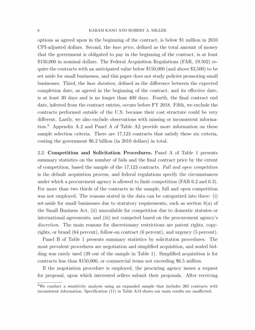
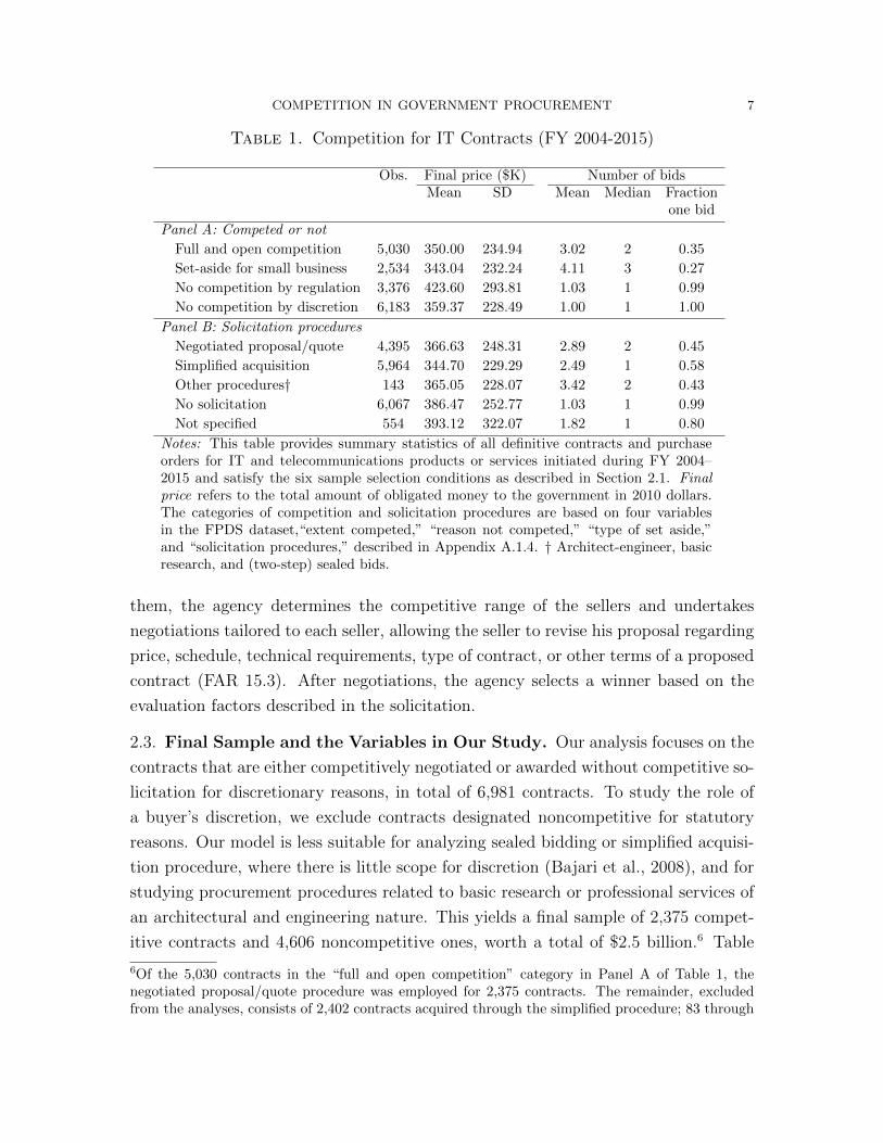
2.2. Competition and Solicitation Procedures. Panel A of Table 1 presents
summary statistics on the number of bids and the final contract price by the extent
of competition, based the sample of the 17,123 contracts. Full and open competition
is the default acquisition process, and federal regulations specify the circumstances
under which a procurement agency is allowed to limit competition (FAR 6.2 and 6.3).
For more than two thirds of the contracts in the sample, full and open competition
was not employed. The reasons stated in the data can be categorized into three: (i)
set-aside for small businesses due to statutory requirements, such as section 8(a) of
the Small Business Act, (ii) unavailable for competition due to domestic statutes or
international agreements, and (iii) not competed based on the procurement agency’s
discretion. The main reasons for discretionary restrictions are patent rights, copy-
rights, or brand (64 percent), follow-on contract (6 percent), and urgency (5 percent).
Panel B of Table 1 presents summary statistics by solicitation procedures. The
most prevalent procedures are negotiation and simplified acquisition, and sealed bid-
ding was rarely used (39 out of the sample in Table 1). Simplified acquisition is for
contracts less than $150,000, or commercial items not exceeding $6.5 million.
If the negotiation procedure is employed, the procuring agency issues a request
for proposal, upon which interested sellers submit their proposals. After receiving
5We conduct a sensitivity analysis using an expanded sample that includes 265 contracts withinconsistent information. Specification (11) in Table A13 shows our main results are unaffected.
COMPETITION IN GOVERNMENT PROCUREMENT 7
Table 1. Competition for IT Contracts (FY 2004-2015)
Obs. Final price ($K) Number of bidsMean SD Mean Median Fraction
one bid
Panel A: Competed or not
Full and open competition 5,030 350.00 234.94 3.02 2 0.35
Set-aside for small business 2,534 343.04 232.24 4.11 3 0.27
No competition by regulation 3,376 423.60 293.81 1.03 1 0.99
No competition by discretion 6,183 359.37 228.49 1.00 1 1.00
Panel B: Solicitation procedures
Negotiated proposal/quote 4,395 366.63 248.31 2.89 2 0.45
Simplified acquisition 5,964 344.70 229.29 2.49 1 0.58
Other procedures† 143 365.05 228.07 3.42 2 0.43
No solicitation 6,067 386.47 252.77 1.03 1 0.99
Not specified 554 393.12 322.07 1.82 1 0.80
Notes: This table provides summary statistics of all definitive contracts and purchaseorders for IT and telecommunications products or services initiated during FY 2004–2015 and satisfy the six sample selection conditions as described in Section 2.1. Finalprice refers to the total amount of obligated money to the government in 2010 dollars.The categories of competition and solicitation procedures are based on four variablesin the FPDS dataset,“extent competed,” “reason not competed,” “type of set aside,”and “solicitation procedures,” described in Appendix A.1.4. † Architect-engineer, basicresearch, and (two-step) sealed bids.
them, the agency determines the competitive range of the sellers and undertakes
negotiations tailored to each seller, allowing the seller to revise his proposal regarding
price, schedule, technical requirements, type of contract, or other terms of a proposed
contract (FAR 15.3). After negotiations, the agency selects a winner based on the
evaluation factors described in the solicitation.
2.3. Final Sample and the Variables in Our Study. Our analysis focuses on the
contracts that are either competitively negotiated or awarded without competitive so-
licitation for discretionary reasons, in total of 6,981 contracts. To study the role of
a buyer’s discretion, we exclude contracts designated noncompetitive for statutory
reasons. Our model is less suitable for analyzing sealed bidding or simplified acquisi-
tion procedure, where there is little scope for discretion (Bajari et al., 2008), and for
studying procurement procedures related to basic research or professional services of
an architectural and engineering nature. This yields a final sample of 2,375 compet-
itive contracts and 4,606 noncompetitive ones, worth a total of $2.5 billion.6 Table
6Of the 5,030 contracts in the “full and open competition” category in Panel A of Table 1, thenegotiated proposal/quote procedure was employed for 2,375 contracts. The remainder, excludedfrom the analyses, consists of 2,402 contracts acquired through the simplified procedure; 83 through
8 KARAM KANG AND ROBERT A. MILLER
2 provides the summary statistics of the various attributes of these contracts, and
Appendix A.1 describes how each of the variables in the table are constructed.
We construct price and duration variables from the entries for each contract. The
base price and the base duration, as defined in Section 2.1, are from the initial entry
of a contract; the final price is the sum of all amounts of money that the government
is obligated to pay across all entries; the final duration is the difference between the
expected completion date as of the last entry and the initial effective date of the con-
tract. The total price adjustment is the difference between the final and base price,
the sum of three types of price adjustments. These depend on the reasons for adjust-
ment: (i) work changes, such as new agreements for additional work, supplementary
agreements, change orders, or termination; (ii) exercise of options or funding issues;
(iii) administrative actions such as seller address changes. The duration adjustments
are similarly defined.7
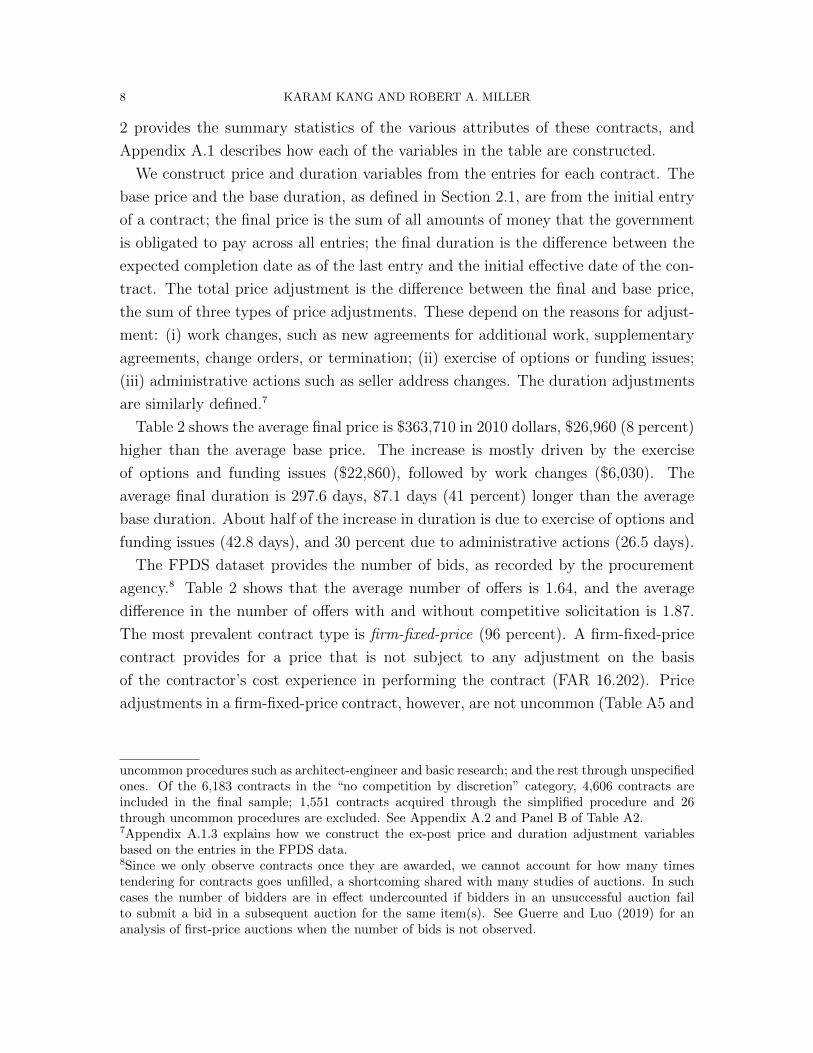
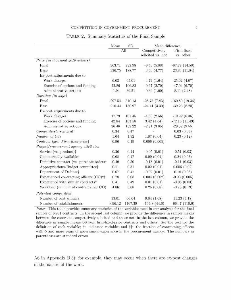
Table 2 shows the average final price is $363,710 in 2010 dollars, $26,960 (8 percent)
higher than the average base price. The increase is mostly driven by the exercise
of options and funding issues ($22,860), followed by work changes ($6,030). The
average final duration is 297.6 days, 87.1 days (41 percent) longer than the average
base duration. About half of the increase in duration is due to exercise of options and
funding issues (42.8 days), and 30 percent due to administrative actions (26.5 days).
The FPDS dataset provides the number of bids, as recorded by the procurement
agency.8 Table 2 shows that the average number of offers is 1.64, and the average
difference in the number of offers with and without competitive solicitation is 1.87.
The most prevalent contract type is firm-fixed-price (96 percent). A firm-fixed-price
contract provides for a price that is not subject to any adjustment on the basis
of the contractor’s cost experience in performing the contract (FAR 16.202). Price
adjustments in a firm-fixed-price contract, however, are not uncommon (Table A5 and
uncommon procedures such as architect-engineer and basic research; and the rest through unspecifiedones. Of the 6,183 contracts in the “no competition by discretion” category, 4,606 contracts areincluded in the final sample; 1,551 contracts acquired through the simplified procedure and 26through uncommon procedures are excluded. See Appendix A.2 and Panel B of Table A2.7Appendix A.1.3 explains how we construct the ex-post price and duration adjustment variablesbased on the entries in the FPDS data.8Since we only observe contracts once they are awarded, we cannot account for how many timestendering for contracts goes unfilled, a shortcoming shared with many studies of auctions. In suchcases the number of bidders are in effect undercounted if bidders in an unsuccessful auction failto submit a bid in a subsequent auction for the same item(s). See Guerre and Luo (2019) for ananalysis of first-price auctions when the number of bids is not observed.
COMPETITION IN GOVERNMENT PROCUREMENT 9
Table 2. Summary Statistics of the Final Sample
Mean SD Mean difference:All Competitively Firm-fixed
solicited vs. not vs. other
Price (in thousand 2010 dollars)
Final 363.71 232.98 -9.43 (5.88) -87.78 (14.58)
Base 336.75 188.77 -3.63 (4.77) -23.83 (11.84)
Ex-post adjustments due to
Work changes 6.03 65.01 -4.74 (1.64) -25.02 (4.07)
Exercise of options and funding 22.86 106.82 -0.67 (2.70) -47.04 (6.70)
Administrative actions -1.94 39.51 -0.39 (1.00) 8.11 (2.48)
Duration (in days)
Final 297.54 310.13 -28.73 (7.83) -160.80 (19.36)
Base 210.44 130.97 -24.41 (3.30) -39.23 (8.20)
Ex-post adjustments due to
Work changes 17.79 101.45 -4.83 (2.56) -19.92 (6.36)
Exercise of options and funding 42.84 183.58 3.42 (4.64) -72.13 (11.49)
Administrative actions 26.46 152.22 -2.91 (3.85) -29.52 (9.55)
Competitively solicited† 0.34 0.47 - 0.03 (0.03)
Number of bids 1.64 1.92 1.87 (0.04) 0.23 (0.12)
Contract type: Firm-fixed-price† 0.96 0.19 0.006 (0.005) -
Project/procurement agency attributes
Service (vs. product)† 0.26 0.44 -0.05 (0.01) -0.51 (0.03)
Commercially available† 0.68 0.47 0.09 (0.01) 0.24 (0.03)
Definitive contract (vs. purchase order)† 0.49 0.50 -0.18 (0.01) -0.11 (0.03)
Appropriations/Budget committee† 0.11 0.31 0.02 (0.01) 0.006 (0.02)
Department of Defense† 0.67 0.47 -0.02 (0.01) 0.18 (0.03)
Experienced contracting officers (CO)†† 0.78 0.08 0.004 (0.002) -0.03 (0.005)
Experience with similar contracts† 0.41 0.49 0.01 (0.01) -0.05 (0.03)
Workload (number of contracts per CO) 4.86 3.08 0.25 (0.08) -0.73 (0.19)
Potential competition
Number of past winners 33.01 66.64 9.84 (1.68) 11.23 (4.18)
Number of establishments 696.12 1767.39 -164.8 (44.6) -664.7 (110.6)
Notes: This table provides summary statistics of the variables used in our analysis for the finalsample of 6,981 contracts. In the second last column, we provide the difference in sample meansbetween the contracts competitively solicited and those not; in the last column, we provide thedifference in sample means between firm-fixed-price contracts and others. See the text for thedefinition of each variable; †: indicator variables and ††: the fraction of contracting officerswith 5 and more years of government experience in the procurement agency. The numbers inparentheses are standard errors.
A6 in Appendix B.3); for example, they may occur when there are ex-post changes
in the nature of the work.
10 KARAM KANG AND ROBERT A. MILLER
We construct ten variables to account for contract-specific observed heterogeneity.
Four variables relate to the nature of the project. First, the project is for products (74
percent) or services, as designated by the FPDS Product and Service Code. Second,
the product or service is either commercially available (68 percent) or not, as deter-
mined by the procurement agency. Third, about half of the contracts in our sample
are definitive contracts, as opposed to purchase orders. Definitive contracts result
from more intensive and specialized contracting, and the agency has little discretion
over these two award types (Warren, 2014). Fourth, we look at the Congressional
representation of the project location, focusing on the members of Congress who are
in charge of the government budgeting and appropriations process: specifically, House
Speakers, majority/minority leaders and whips, and chairmen or ranking members of
the Committees on the Budget, Appropriations, and Ways and Means. The locations
of 11 percent of the contracts were represented by such members.
Four variables capture observed heterogeneity in procurement agencies, which we
aggregate to the level of the 15 cabinet executive departments or the 13 federal inde-
pendent agencies. First, the Department of Defense (DoD) accounts for 67 percent of
the contracts. The second variable is the fraction of the agency’s contracting officers
with at least 5 years of federal government experience. The third variable indicates
whether the agency handled in the past three years a similar contract in the sense
that Product and Service code, commercial availability, contract instrument (defini-
tive contract or purchase order), and the state of the project location are the same.
The fourth variable measures the amount of workload when the contract was signed,
by the number of definitive contracts and purchase orders of size greater than $25,000
initiated during the fiscal year, per contracting officer of the agency.
The remaining two variables measure the extent of potential competition for each
contract. First, we count the number of unique winners of the contracts that (i) are
similar (as specifically defined above) to a given contract; (ii) were signed by the
DoD (if the contract is also signed by that department) or other agencies (otherwise)
in the past three years. The average number of such past winners is 33.01, but the
distribution is skewed: 21 percent of contracts are associated with at most one past
winner. Second, acknowledging that the first measure is likely to underestimate the
level of potential competition by excluding losing contractors, we cast a wider net
by computing the number of establishments that have the same North American
Industry Classification System (NAICS) code and are located in the same state as
the winner of a given contract during the year that the contract was signed.
COMPETITION IN GOVERNMENT PROCUREMENT 11
2.4. Endogenous Competition and Contract Type. As discussed in Section 2.2,
procurement agencies have discretion over whether to solicit competitive bids or not.
Contracting officers must provide and certify the justification for not competitively
soliciting bids. Approval by another official is required only if the contract size is
over $0.7 million (FAR 6.3). We reviewed the justification documents associated
with our sample, as available on the federal business opportunities website (www.
fbo.gov).9 Each document includes a section that provides qualitative reasons for
not engaging in full and open competition (in 2.9 paragraphs on average). These
documents sometimes acknowledge other sellers providing similar items.10
Procurement agencies also determine the extent to which they seek and exchange
information with potential sellers, via pre-solicitation notices, requests for informa-
tion, draft requests for proposals, public hearings, and market research, before issuing
the actual solicitation. Furthermore, evaluating an additional bid incurs an extra ad-
ministrative burden, and there is even anecdotal evidence that the risk of receiving a
bid protest from losing sellers is nontrivial.11
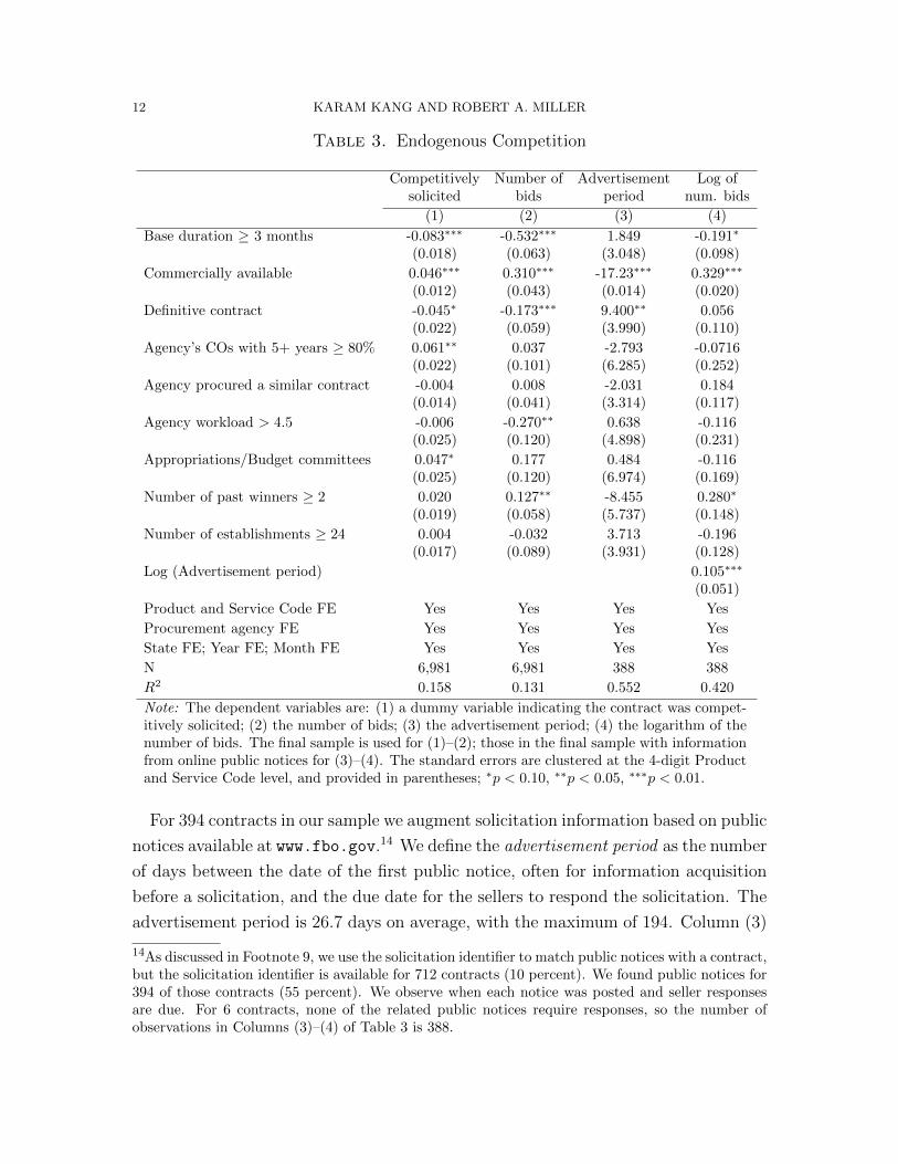
These institutional features suggest that demand factors affect the number of bids.
We regress the number of bids on contract attributes, and Column (2) of Table 3
shows the greater the procurement agency’s workload, the fewer the bids.12 Column
(1) shows when more experienced contracting officers are employed in the agency,
competitive solicitation is more likely. These findings are consistent with the notion
that it is costly to acquire the market information and to wait for more bids.13
9We track the Justification and Approval (J&A) document for each contract by searching for publicnotices at www.fbo.gov. We match a public notice to a contract by the solicitation identifier, butthat information is not required for contracting officers to provide for the FPDS dataset. As a result,we observe the identifier for only 40 noncompetitive contracts (1 percent); among that subset weidentified public notices for 23 contracts, including 11 J&A documents in total.10For example, the J&A document regarding VA11812Q0632 posted in September 2012 states: “Al-though other vendors provide similar imaging software, only iNtuition brand name software, throughits use of the “thin client” server technology, meets this capability.”11Federal Times reported in July 2013 on how bid protests are slowing down procurements. Thearticle quoted Mary Davie, assistant commissioner of the Office of Integrated Technology Servicesat the General Services Administration: “We build time in our procurement now for protests. Weknow we are going to get protested.”12In all the Table 3 regressions, we control for the ten contract attributes as described in Section2.3, as well as fixed effects for four-digit Product and Service code; procurement agency; fiscal yearand month contact is signed (Liebman and Mahoney, 2017); location of project by state.13In addition, Table A4 in Appendix B.2 shows that using instruments eliminate the positive elas-ticity between price and the number of bids obtained in an OLS regression.
12 KARAM KANG AND ROBERT A. MILLER
Table 3. Endogenous Competition
Competitively Number of Advertisement Log ofsolicited bids period num. bids
(1) (2) (3) (4)
Base duration ≥ 3 months -0.083∗∗∗ -0.532∗∗∗ 1.849 -0.191∗
(0.018) (0.063) (3.048) (0.098)
Commercially available 0.046∗∗∗ 0.310∗∗∗ -17.23∗∗∗ 0.329∗∗∗
(0.012) (0.043) (0.014) (0.020)
Definitive contract -0.045∗ -0.173∗∗∗ 9.400∗∗ 0.056(0.022) (0.059) (3.990) (0.110)
Agency’s COs with 5+ years ≥ 80% 0.061∗∗ 0.037 -2.793 -0.0716(0.022) (0.101) (6.285) (0.252)
Agency procured a similar contract -0.004 0.008 -2.031 0.184(0.014) (0.041) (3.314) (0.117)
Agency workload > 4.5 -0.006 -0.270∗∗ 0.638 -0.116(0.025) (0.120) (4.898) (0.231)
Appropriations/Budget committees 0.047∗ 0.177 0.484 -0.116(0.025) (0.120) (6.974) (0.169)
Number of past winners ≥ 2 0.020 0.127∗∗ -8.455 0.280∗
(0.019) (0.058) (5.737) (0.148)
Number of establishments ≥ 24 0.004 -0.032 3.713 -0.196(0.017) (0.089) (3.931) (0.128)
Log (Advertisement period) 0.105∗∗∗
(0.051)
Product and Service Code FE Yes Yes Yes Yes
Procurement agency FE Yes Yes Yes Yes
State FE; Year FE; Month FE Yes Yes Yes Yes
N 6,981 6,981 388 388
R2 0.158 0.131 0.552 0.420
Note: The dependent variables are: (1) a dummy variable indicating the contract was compet-itively solicited; (2) the number of bids; (3) the advertisement period; (4) the logarithm of thenumber of bids. The final sample is used for (1)–(2); those in the final sample with informationfrom online public notices for (3)–(4). The standard errors are clustered at the 4-digit Productand Service Code level, and provided in parentheses; ∗p < 0.10, ∗∗p < 0.05, ∗∗∗p < 0.01.
For 394 contracts in our sample we augment solicitation information based on public
notices available at www.fbo.gov.14 We define the advertisement period as the number
of days between the date of the first public notice, often for information acquisition
before a solicitation, and the due date for the sellers to respond the solicitation. The
advertisement period is 26.7 days on average, with the maximum of 194. Column (3)
14As discussed in Footnote 9, we use the solicitation identifier to match public notices with a contract,but the solicitation identifier is available for 712 contracts (10 percent). We found public notices for394 of those contracts (55 percent). We observe when each notice was posted and seller responsesare due. For 6 contracts, none of the related public notices require responses, so the number ofobservations in Columns (3)–(4) of Table 3 is 388.
COMPETITION IN GOVERNMENT PROCUREMENT 13
of Table 3 presents the regression results explaining the advertisement period. They
suggest that procurement agencies exert more search efforts on contracts that they
expect to have a smaller pool of potential sellers: both commercial availability and
purchase orders (as opposed to definitive contracts) are associated with more bids
and shorter advertisement periods. Column (4) shows that, conditional on contract
attributes, the advertisement period and the number of bids are positively correlated.
The regulations explicitly specify that the contract type is a matter for negotiation,
recognizing the close relationship between final price and contract type (FAR 16.1).15
Based on the 208 available solicitation documents, we find that (i) 26 percent of
them do not specify a contract type; (ii) the contract type in the solicitation is not
always identical to the actual type; (iii) even when the contract type is specified in
the solicitation, the wording is not always definitive, stating that the government
“intends to,” “contemplates,” or “anticipates” that the resulting contract will be a
firm-fixed-price contract, for example.16
2.5. Repeated Interaction. We believe the scope for repeated interactions between
the procurement agency and sellers is limited. First, Table 2 shows that for 59 percent
of the contracts, the procurement agency does not have experience of procuring a
similar contract to the contract in question within the past three years.17 Second,
Table 3 shows the procurement agency’s experience of dealing with a similar contract
is not correlated with the extent of competition.18 Third, most sellers win only one
contract during the period of study (Table A3 in Appendix B.1).
Our capacity to study collusion and reputation is limited; we observe the number
of losing bids, but not their identities. However, the contracts in our sample tend to
appear irregularly in terms of size and requirements. Coupled with the aforementioned
point that most sellers win only once, these features make it difficult for sellers to
maintain a collusive relationship (Porter and Zona, 1993). Although the data are
15FAR 16.103(a) states: “Selecting the contract type is generally a matter for negotiation andrequires the exercise of sound judgement. Negotiating the contract type and negotiating prices areclosely related and should be considered together.”16Among the 394 contracts that have public notices at www.fbo.gov, we retrieved the solicitationdocuments for only 208 contracts, mainly because the link to the documents was broken.17In addition, a report of the US Government Accountability Office in 2009 (GAO-09-374) concludesthat contracting officials are reluctant to rely more on past performance, partly because they areskeptical of the reliability of information and find it difficult to assess relevance to specific acquisition.18On the flip side, Appendix B.1 shows that repeat sellers, those who have won contracts multipletimes, do not necessarily face less competition than those who have not.

14 KARAM KANG AND ROBERT A. MILLER
unsuitable for studying intertemporal incentives, we partially accommodate long-term
relationships of buyer-seller pairs through buyer preferences for no competition.
3. Model
3.1. Setup. The institutional features profiled in Section 2 guide our model. Suppose
a buyer is assigned to administer a procurement process for a government project.
There are two types of sellers, denoted by k ∈ 0, 1.19 The proportion of the second
type in the population, denoted by π ∈ (0, 1), is common knowledge to the buyer
and the sellers. The total cost to a type k seller of completing the project is the
sum of a type-specific initial cost, γk, plus an uncertain component. The latter
component depends on contractible outcomes, denoted by s, realized and observed by
both parties after the project is completed, according to fk(s), a probability density
function conditional on seller type. We denote the cost component determined by
contractible outcomes by c(s). The expected cost of a type k seller is denoted by ck:
ck ≡ γk +
∫c(s)fk(s)ds.
The first seller type is designated high-cost, the second low-cost, and we assume
γ1 < γ0 and
∫c (s) f1(s)ds <
∫c (s) f0(s)ds. (1)
We assume γk is hidden information, known to the seller only, and therefore not
contractible. We assume that s is informative but imperfect: f0(s) 6= f1(s) for some
s, but share a common support.
The solicitation rules described in Section 2.2 delegate responsibility to the buyer
for deciding whether she will permit competition or not. If a buyer solicits competitive
bids, as opposed to contracting with a default seller, there is a cost, η.20 Regardless of
whether she solicits competitive bids or not, the buyer designs a menu of contracts.
Each contract in the menu is contingent on the number of sellers n ∈ 1, 2, . . .who might bid. If she solicits competitive bids the buyer chooses how intensely to
19In the equilibrium menu derived in Theorem 3.1, there are as many seller types as there arecontract types. As explained in Section 2.3, we partition contracts into one of two contract types,firm-fixed-price and other, to rationalize this assumption.20The solicitation costs, η, incorporate the value to the buyer from the default seller compared toother sellers. In principle this value might arise from the default seller’s level of specialization match-ing the specific needs of the buyer, concerns about noncontractible project quality from the otherpotential sellers, increased administrative costs incurred from engaging in a competitive solicitationprocess, as well as direct private benefits to the buyer from awarding the contract to the defaultseller, including bribery and corruption stemming from favoritism.

COMPETITION IN GOVERNMENT PROCUREMENT 15
search for sellers if she permits competition, defined as the arrival rate of a Poisson
distribution for the number of bids, λ ∈ R+, at the cost of κλ. When a seller arrives,
he selects and submits one contract from those listed on the menu. The buyer awards
the project to a seller whose contract ranks the highest amongst total submissions,
and ties are broken randomly.21
A typical contract denoted by j ∈ 0, 1, . . . , J comprises a base price, which
might depend on the number of sellers, n, we denote by pjn, and a price adjustment,
a mapping denoted by qjn(s). We assume there exists some fixed negative constant M
that bounds the difference qjn(s)− c(s) from below. In theory, this maximal penalty
finesses situations where it might otherwise be optimal to achieve an outcome very
close to first best, potentially achieved by imposing extremely steep penalties on
low-cost winners for outcomes that would be very unlikely for high-cost sellers. In
practice, M reflects limited liability and seller bankruptcy constraints.
The buyer is risk neutral. Denoting the winning contract by pin, qin(s), the total
cost of procurement is:pin + qin(s) + κλ+ η if the buyer solicits competition with intensity λ,
pi1 + qi1(s) if she contracts with a default seller.(2)
The seller can be risk averse. Liquidity concerns, or the cost of working capital, lead
him to discount (enlarge) positive (negative) deviations from a contract that offers
full insurance.22 The payoff to a type k seller from winning pin, qin(s) is:
pin − γk + ψ [qin(s)− c(s)] , (3)
where ψ (·) : R → R is continuous, with ψ(0) = 0, ψ′(0) = 1, and for any r ∈ R,
ψ′(r) > 0 and ψ′′(r) ≤ 0. Losing sellers receive a payoff of zero, as do sellers who opt
out of the procurement process.
Summarizing the event sequence, first the buyer chooses whether to solicit compet-
itive bids. At that time she also forms a contract menu, pjn, qjn(s)Jj=0 including a
21An alternative model for negotiation is generalized Nash bargaining, which may be appropriate fora situation where there is a natural supplier with whom the government has an existing relationshipbased on past dealings. Given that in our data more than 50 percent of the winners only win once(Table A3 in Appendix B.1), this situation does not seem to apply to our data.22The price adjustments can be costly, potentially due to adaptation costs (Crocker and Reynolds,1993; Bajari and Tadelis, 2001; Bajari et al., 2014) and sellers’ risk aversion (Baron and Besanko,1987; Laffont and Rochet, 1998; Arve and Martimort, 2016). Arve and Martimort (2016) explicitlymodel firms’ risk aversion in a procurement context. See pages 3240–3241 for their justifications,including imperfect risk management or diversification, bankruptcy or auditing cost of issuing debt,liquidity constraints, nonlinear tax systems, and internal agency problems.
16 KARAM KANG AND ROBERT A. MILLER
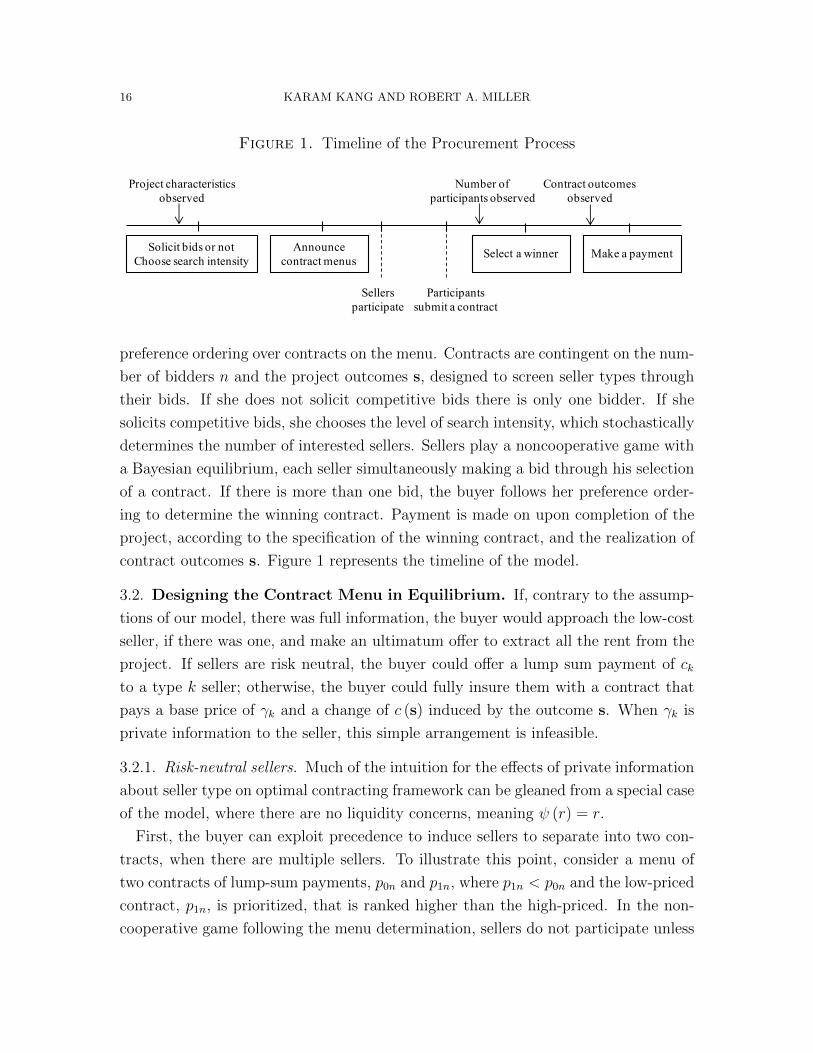
Figure 1. Timeline of the Procurement Process
Sellers
participate
Participants
submit a contract
Project characteristics
observed
Number of
participants observed
Contract outcomes
observed
Solicit bids or not
Choose search intensity
Announce
contract menusSelect a winner Make a payment
preference ordering over contracts on the menu. Contracts are contingent on the num-
ber of bidders n and the project outcomes s, designed to screen seller types through
their bids. If she does not solicit competitive bids there is only one bidder. If she
solicits competitive bids, she chooses the level of search intensity, which stochastically
determines the number of interested sellers. Sellers play a noncooperative game with
a Bayesian equilibrium, each seller simultaneously making a bid through his selection
of a contract. If there is more than one bid, the buyer follows her preference order-
ing to determine the winning contract. Payment is made on upon completion of the
project, according to the specification of the winning contract, and the realization of
contract outcomes s. Figure 1 represents the timeline of the model.
3.2. Designing the Contract Menu in Equilibrium. If, contrary to the assump-
tions of our model, there was full information, the buyer would approach the low-cost
seller, if there was one, and make an ultimatum offer to extract all the rent from the
project. If sellers are risk neutral, the buyer could offer a lump sum payment of ck
to a type k seller; otherwise, the buyer could fully insure them with a contract that
pays a base price of γk and a change of c (s) induced by the outcome s. When γk is
private information to the seller, this simple arrangement is infeasible.
3.2.1. Risk-neutral sellers. Much of the intuition for the effects of private information
about seller type on optimal contracting framework can be gleaned from a special case
of the model, where there are no liquidity concerns, meaning ψ (r) = r.
First, the buyer can exploit precedence to induce sellers to separate into two con-
tracts, when there are multiple sellers. To illustrate this point, consider a menu of
two contracts of lump-sum payments, p0n and p1n, where p1n < p0n and the low-priced
contract, p1n, is prioritized, that is ranked higher than the high-priced. In the non-
cooperative game following the menu determination, sellers do not participate unless
COMPETITION IN GOVERNMENT PROCUREMENT 17
their expected utility is weakly positive. So to guarantee the project is undertaken,
p0n ≥ c0. This inequality can be modeled as an individual rationality constraint on
the buyer relating to high-cost sellers (IR0), and Lemma A1 in Appendix C proves
IR0 binds: p0n = c0. Analogous reasoning motivates an individual rationality con-
straint for the low-cost sellers (IR1), namely p1n ≥ c1. Thus c0 is offered to high-cost
sellers, and buyer offers some lower price p1n ∈ [c1, c0) to low-cost sellers. To induce
low-cost sellers to bid p1n the expected value from doing so must be at least as great
as the expected value from p0n. Define φ1n, the winning probability if he chooses p1n
when the other sellers follow the same equilibrium strategy, as:
φ1n ≡n−1∑i=0
(n− 1
i
)πi(1− π)n−1−i
i+ 1=
1
nπ
n∑i=1
(n
i
)πi(1− π)n−i =
1− (1− π)n
nπ. (4)
If he chooses p0n instead, the probability of winning is:
φ0n ≡ n−1(1− π)n−1. (5)
Thus a low-cost seller prefers p1n to p0n if and only if:
φ1n (p1n − c1) ≥ φ0n (c0 − c1) . (6)
We treat (6) as an incentive compatibility constraint for the low-cost seller (IC1) that
the buyer must respect when designing the menu. Note that IC1 must bind when
IR1 does not; otherwise p1n could be reduced without violating either constraint and
reducing the expected amount of the buyer’s payment to a winning seller. Making
p1n the subject of the resulting equality and simplifying:
p1n = c1 +π(1− π)n−1
1− (1− π)n(c0 − c1) .
Thus p1n declines in n, converging to c1 and replicating a first-price sealed-bid auction
with reservation price c0. When n = 1, this menu reduces to a pooling equilibrium,
but when n > 1, it is separating, p1n < c0, and hence the expected payment is strictly
less than the pooling menu that satisfies IR0, namely c0.
Second, exploiting contract outcomes to further penalize the low-cost seller from
deviating to the high-cost contract gives the buyer more leverage to extract rent from
the low-cost seller. Intuitively, the contract for the high-cost seller is designed to
discourage the low-cost seller from choosing it, by rewarding outcomes that are more
likely to occur when a high-cost seller wins the project, and penalizing outcomes that
are more likely if the low-cost seller had chosen the high-cost contract and won the
18 KARAM KANG AND ROBERT A. MILLER
project. For example, define:
r (s) ≡
(γ0 − γ1)/∫f0(s)≥f1(s)
[f0(s)− f1(s)] ds +M if f1 (s) ≤ f0 (s) ,
M otherwise,
and set a menu of two contracts, consisting of p1n, q1n (s) = c1, 0 and p0n, q0n (s) =c0 −
∫[r (s) + c (s)]f0(s)ds, r (s) + c (s)
. By inspection, the menu satisfies all con-
straints: IC0 does not bind; IC1 binds as does IR1 and IR0; the limited liability
does not bind if f1 (s) ≤ f0 (s) and binds otherwise. Under this menu, the buyer can
extract all the seller surplus. Thus, given any number of sellers, the buyer offers a
separating menu that exploits information from contract outcomes.
3.2.2. Risk-averse sellers. The intuition from the risk-neutral sellers can be extended
to situations in which ψ (r) is strictly concave. Some additional notation helps. Let
l (s) ≡ f1(s)/f0(s) denote the likelihood ratio, and define the threshold likelihood
ratio associated with the limited liability condition by:
l(π) ≡ 1
π− 1− ππψ′ (M)
. (7)
Lemma A6 in Appendix C proves there is at most one root in π ∈ (0, 1) to the
following expression:
γ0−γ1−∫ψ
(ψ′−1
[1− π
1− πl(s)
]1l(s) ≤ l(π)+M1l(s) > l(π)
)[f0(s)− f1 (s)] ds.
(8)
We denote the root by π when it exists, and otherwise set π = 1.
Theorem 3.1. Let:
r (s) ≡
ψ′−1(
1−minπ,π1−l(s) minπ,π
)if l(s) ≤ l(min π, π),
M if l(s) > l(min π, π),(9)
pn ≡ γ1 +π (1− π)n−1
1− (1− π)n
(γ0 − γ1 −
∫ψ[r (s)] [1− l (s)] f0(s)ds
), (10)
p ≡ γ0 −∫ψ[r(s)]f0(s)ds (11)
To minimize her expected costs of procurement the buyer offers a menu of two con-
tracts, given by p1n, q1n (s) = pn, c (s) and p0n, q0n (s) = p, r(s) + c(s), rank-
ing the former above the latter. This menu induces a separating equilibrium amongst
the sellers: sellers of type k submit pkn, qkn (s).

COMPETITION IN GOVERNMENT PROCUREMENT 19
Appendix C contains all the proofs. In the solution to the buyer’s problem p1n
and p0n solve two equations in terms of q1n(s) and q0n(s) that characterize IC1 and
IR0, both of which bind. Low-cost sellers are offered a full insurance contract, where
q1n (s) = c (s). We show from (10), p1n < γ0, so IC0 is not binding. Furthermore, IR1
is satisfied for any π, and is binding when π ≥ π by (8). Substituting the solutions
for p1n and p0n into the expression for the buyer’s cost, we minimize the expected
cost with respect to the remaining contract parameter, q0n(s), subject to the limited
liability constraint.
The solution to the framework with risk-averse sellers share common features with
its risk neutral analogue. First, there is no pooling equilibrium. Second, since ψ′(0) =
1 and its derivative is negative, it follows from (9) that q0n(s) ≷ c(s) as l (s) ≶ 1. In
words, if a certain realized outcome of s is more (less) likely to be generated by a high-
cost seller than a low-cost one, then q0n(s) over-compensates (under-compensates)
cost changes so that low-cost sellers are incentivized not to mimic high-cost ones, as
in the risk neutral case. Third, from (9) and (11), neither p0n and q0n(s) depend on
the number of bids, because IR0 binds in both cases.23
The critical difference between the two scenarios is that when sellers are risk-averse,
the buyer must compensate high-cost sellers with a sufficiently high risk premium for
accepting contracts that do not offer full insurance. For some parameter values, IR1
does not bind in the menu defined in Theorem 3.1. In that case, the expected contract
price designed for low-cost sellers declines with the number of bids, converging to
c1, which can be seen by differentiating (10). This manifests the benefits of more
competition in the risk averse case, and it also contrasts with the risk neutral case,
where the only reason to attract more bidders is to increase the likelihood of attracting
low-cost sellers, not to extract more rent from a low-cost winner.
Given n bids, let T (n) denote the expected payment under the menu of Theorem
3.1; let TU(n) denote the minimal expected payment when the buyer is fully informed
about seller type; and let TFIC(n) denote the minimal expected payment when she
is constrained to offer only full insurance contracts. Corollary 3.1 implies TU(n) <
T (n) < TFIC(n).
23This result is similar to McAfee and McMillan (1987); Laffont and Tirole (1987); Riordan andSappington (1987), where the distortions due to information asymmetry are invariant to the numberof bids, though expected distortions and seller profits decline with the number of bids.
20 KARAM KANG AND ROBERT A. MILLER
Corollary 3.1. For any n ∈ 1, 2, . . .:
T (n) = TFIC(n) + (1− π)n−1 Γ, (12)
TFIC(n) = TU(n) + (1− π)n−1 π (γ0 − γ1) , (13)
TU(n) = c1 + (1− π)n (c0 − c1) , (14)
where:
Γ ≡ (1− π)
∫ r(s)− ψ[r(s)]
f0(s)ds− π
∫ψ[r(s)] [1− l(s)] f0(s)ds. (15)
From (12), note that Γ = T (1)−TFIC(1) < 0. Moreover as n increases, the absolute
value of the difference, (1− π)n−1 Γ, declines at a geometric rate. Intuitively, in her
quest to extract rent from low-cost sellers when faced with the constraint of having
to accept a high-cost seller as a last resort, the buyer uses s to discriminate between
the two types, and that the value of discriminating declines with more bids.
3.3. Soliciting Bids in Equilibrium. Having solved the contract menu and the
expected payments to a winning seller for a given number of bids, the expected total
cost of competitive procurement with search effort λ is thus:
U(λ, η) ≡∞∑n=0
λne−λ
n!T (n+ 1) + κλ+ η, (16)
where T (n) is defined in (12). Because U(λ, η) is convex in λ, it attains an un-
constrained global minimum at its unique stationary point, denoted by λ, and we
denote the optimal search intensity by λo ≡ max0, λ. The expected total cost of
noncompetitive procurement is U(0, 0). Competitive bids are sought if and only if:
U(λo, η) ≤ U(0, 0),
which is equivalent to η ≤ Ω, where
Ω ≡ U(0, 0)−∞∑n=0
(λo)ne−λo
n!T (n+ 1)− κλo
= (1− e−λoπ)
((1− π)(c0 − c1) + π(γ0 − γ1) + Γ
)− κλo. (17)
Note that if λo = 0, then the choice reduces to the sign of η.
COMPETITION IN GOVERNMENT PROCUREMENT 21
3.4. Extensions. Our model can incorporate entry or bid preparation costs borne
by sellers to participate in the procurement process, denoted by κs.24 As in the main
model presented above, if the buyer decides to competitively solicit bids, then she
determines the optimal search intensity, λ, at the cost of κλ, and via the Poisson
process with arrival rate λ, she gets in contact with n sellers. We assume each seller
knows his type as well as the number of sellers that the buyer is in contact with. The
buyer presents a menu to the sellers; each seller decides whether to pay κs or not,
and if so, which item on the menu to select. The rest of the procurement proceeds
as before: the buyer selects a winner, pays a base price when the project begins, and
makes a price adjustment when the contract outcomes are revealed. Corollary 3.2
below solves an optimal menu for this extension.
Corollary 3.2. Given an entry cost of κs and the buyer’s search intensity λ, the equi-
librium menu comprises two contracts,pn + κs
φ1n, c (s)
and
p+ κs
φ0n, r (s) + c (s)
,
where the former is ranked higher, φkn is defined in (4)–(5), and (r (s) , pn, p) is de-
fined in (9)–(11).
The explanation for this modified menu is straightforward. Sellers are not directly
compensated for their entry costs, but when making a bid, they enter a lottery by
paying κs. The lottery prize for winning the contract is κs/φkn for k ∈ 0, 1, and the
lottery is actuarially fair for either seller, appealing to (4)–(5). This form of compensa-
tion gives the appearance of padding initial costs, but is a way of efficiently managing
entry, through the choice of λ, by internalizing the tension between compensating
sellers for their entry costs and the beneficial effects from attracting a greater number
of sellers bidding for the project.
These results add to the literature on endogenous entry in auctions where sellers
pay entry costs (Bajari and Hortacsu, 2003; Hendricks et al., 2003; Li, 2005; Li and
Zheng, 2009; Athey et al., 2011; Krasnokutskaya and Seim, 2011; Athey et al., 2013).
In particular, Li and Zheng (2009) demonstrate that increasing the number of po-
tential bidders can increase the price because a lower probability of winning reduces
the chances of being compensated for entry costs, with such effects dominating the
pressure to decrease the price through greater competition. There is no presumption
in this literature that the equilibrium number of bids tendered is optimal from the
24We assume that the entry costs of sellers are independent of the cost of the project and its quality.Hence procurement of research and innovation, where sellers’ (unverifiable) efforts prior to biddingmay affect the quality (Taylor, 1995; Fullerton and McAfee, 1999; Che and Gale, 2003) is beyond thescope of the model. See Bhattacharya (ming) for an empirical study of R&D procurement contestsin this context.
22 KARAM KANG AND ROBERT A. MILLER
buyer’s perspective. However, giving discretion to the buyer to set rules on how to
determine the winner and the winning bid vests her with the power to internalize this
congestion externality.
Another direction to extend the model is relaxing the assumption that the benefit
from the project to the buyer does not depend on contract outcomes. To be explicit,
we can express the benefits as a mapping b (s). Denote the expected benefit from type
k seller by bk ≡∫b (s) fk(s)ds. Then the ranking of seller types might not depend on
their costs alone. If the expected benefits from a low-cost seller, b1, are at least as
good as a high-cost seller’s, b0, then the buyer ranks low-cost sellers over high-cost
sellers and implements the menu of Theorem 3.1.
Corollary 3.3. The menu defined in Theorem 3.1 is optimal if b1 ≥ b0.
Our model is limited to two seller types. We conjecture that the main properties
of the model apply to extensions with more than two seller types: there is separation,
precedence is inversely related to cost, the lowest cost seller is fully insured, and
the individual rationality constraint for the highest cost seller binds. In this way
the framework captures the essentials of a more general problem, but counterfactual
predictions might be sensitive to the number of seller types.
One aspect left for future research is a role for moral hazard in this framework.
Considering the simplest case, suppose there is hidden information about both seller
type (high-cost or low-cost), and the agent’s actions (work or shirk) affect the prob-
ability distribution of outcomes. Then, similar to Gayle and Miller (2015), necessary
conditions for an optimal menu designed to induce both seller-types to work would be
to respect additional incentive compatibility constraints that lead each seller-type to
prefer working and announcing their true type to choosing alternative effort combi-
nation and pretending to be the other seller type. In equilibrium, price adjustments
would reflect the effects of multiple likelihood ratios formed from the probability den-
sities for contract outcomes with different seller types and effort choices. No contract
would offer full insurance (because of the moral hazard aspect), but a characterization
of even the qualitative properties would depend on a relatively detailed specification
of the underlying outcome distributions. Complicating matters still further, our data
does not include records of on-the-job monitoring or auditing.25 For these reasons we
25Contracting officers in the agency have authority to enter into, administer, or terminate contracts(FAR 1.602), but they may delegate contract administration to another government agency (FAR42.202). A government audit agency is responsible for analyzing the financial and accounting recordsof a contractor to determine the incurred and estimated costs and for reviewing the contractor’s cost
COMPETITION IN GOVERNMENT PROCUREMENT 23
do not pursue the analysis of a framework with both hidden information and hidden
action components.
4. Identification
The distribution of contract outcomes, the risk preferences of sellers, the propor-
tion of the low-cost type, the cost structure of both seller types, the buyer’s search
costs, and her preference for competitive contracting, comprise the primitives of the
model. Rather than viewing π, the proportion of low-cost sellers, as a parameter
to be estimated, we treat π as a project-specific unobserved random variable drawn
from a probability distribution Fπ, a nondecreasing and continuously differentiable
mapping from Π ⊂ (0, 1) to [0, 1]. Initial project costs depend on π through γk (π),
a differentiable mapping from Π to R+; likewise we model search costs κ (π), as a
continuous mapping from Π to R+. The density functions of s ∈ S, f0 and f1, belong
to the set of continuous probability density functions, and the distribution function of
the unobserved random variable η, is denoted by Fη, a nondecreasing function defined
from R to [0, 1]. Cost changes c (s) are a mapping from S to R. Risk preferences are
represented by ψ, a twice differentiable concave function from R to R tangent to the
identity function at the origin.
We assume the data generating process of the model records: whether the contract
draws competitive bids, denoted by setting y = 1, or not (setting y = 0); the number
of bids, n; the winning contract type, k ∈ 0, 1; contract outcomes, s; the base price
of the winning contract pkn, and price adjustments qk(s), which depend on contract
outcomes and the winning contract type.26 We provide assumptions and notation,
and establish three monotonicity results underpinning the identification. Then we
describe an intuitive explanation of our identification strategy, followed by a step-by-
step elaboration. Proofs not given in the text are provided in Appendix D.
4.1. Assumptions and Notation. To identify the model we assume:
A1.: s, π, and η are mutually independent.
A2.: Fπ (π) is strictly increasing for all π ∈ Π.
A3.: Π ⊂ (0, π), and l (s) ≤ l(π) for all (s, π) ∈ S × Π.
A4.: γ1 (π) is non-increasing in π ∈ Π.
control systems (FAR 42.101). Furthermore, monitoring contractor compliance with contractualrequirements must occur as part of the quality assurance procedures (FAR 46).26We use the same notation k to denote the seller type and the contract type because the equilibriumis separating, which provides a one-to-one mapping between the seller type and the contract type.For this reason, we call p1n, q1n a low-cost contract and p0n, q0n a high-cost contract.
24 KARAM KANG AND ROBERT A. MILLER
A5.: γ0 (π)− γ1 (π) is non-increasing in π ∈ Π.
A6.: Either Ψ0 (π) ≤ γ′0 (π) for all π ∈ Π, or Ψ0 (π) ≥ γ′0 (π) for all π ∈ Π where:
Ψ0 (π) ≡∫ (
ψ′′[ψ′−1
(1− π
1− πl(s)
)])−1(1− π) [l(s)− 1]
[1− πl(s)]3f0(s)ds.
To facilitate the exposition we define v (l, π) as the interior solution to r in the
optimality condition given by (9):
ψ′(r) =1− π1− πl
. (18)
Assuming A3 implies from Theorem 3.1 that v (l (s) , π) = q0n (s)−c (s) for all π ∈ Π.
For notational convenience we also make explicit the dependence of the base price
variables p and pn on π by writing p (π) and pn (π) respectively.
Assumption A1 can be relaxed if suitable instruments are available. Our empirical
implementation allows for correlation between π and η using an instrumental variables
approach, and our approach to identification can be extended to account for such
correlations.27 We appeal to A2 when connecting the probability distribution of pn,
conditional on n, with the probability distribution of π conditional on a low-cost seller
winning. It is essentially a technical condition finessing situations where fπ (π∗) = 0
for some π∗ and hence no observations exist for pn (π∗). A3 means that neither
IR1 nor the limited liability constraint bind, implying (18) holds. Our parametric
specification relaxes this assumption in estimation. Assumptions A4 and A5 bound
the derivatives of base costs with respect to π, and include the notable specialization
that initial costs do not depend on π. These bounds are not tight, and we do not
impose them in the estimation. Our proof of identification also shows that if ψ (r)
is known, then the remaining parameters are over-identified from Assumptions A1
through A5 alone. Thus A6 is a uniformity assumption jointly restricting the space
of risk preferences and the distribution of outcomes, only used in the identification
of ψ (r). Summarizing, these assumptions are collectively sufficient but not necessary
for identifying the primitives; they provide guidelines for estimation, and serve as a
27By way of contrast, we do not relax the assumption that s is independent of π and η. If the contractoutcome distributions for each seller type k = 0, 1 vary with (π, η) so that fk(s|π, η) 6= fk(s), thenfk(s|π, η) is not identified from data on contract outcomes and seller type alone because π and η areunobserved. Our approach is to identify f0(s) and f1(s) first from the observed contract outcomesconditional on seller type, and exploit this feature throughout. However if the distribution of sdepends on (π, η), the buyer duly accounts for this dependence in her menu design. Ignoring it whenaggregating across projects of different types could bias counterfactual predictions.
COMPETITION IN GOVERNMENT PROCUREMENT 25
point of departure for restricting the parameter space along some dimensions in order
to enlarge it on others, depending on the specificities of the dataset.
4.2. Monotonicity. The proof of identification exploits monotonicity properties. As
π increases, there is a greater chance of selecting a low-cost seller and thus the buyer
can reduce the base price for the low-cost contract if IR1 does not bind already. We
show that ∂pn(π) /∂π < 0 for all n ∈ 1, 2, . . . given A3–A5. We show that to
satisfy IC1 while reducing pn(π) as π increases, the buyer increases the volatility
of the high-cost contract, making it less attractive to low-cost sellers, which is to
say ∂ |v(l, π)| /∂π > 0. Whether the increased volatility makes the high-cost contract
more or less attractive to high-cost sellers depends on the other primitives; we provide
conditions for monotonicity of p(π) in π.
Lemma 4.1. (i) If A3 holds then ∂ |v(l, π)| /∂π > 0. (ii) If A3–A5 hold then
∂pn(π) /∂π < 0 for all n ∈ 1, 2, . . .. (iii) If A3 and A6 hold then p (π) is monotone.
4.3. Overview. Because the equilibrium menu separates low-cost from high-cost sell-
ers, the densities for contract outcomes, f1(s) and f0(s), are identified. Since the
menu offers full-insurance to low-cost sellers, cost changes are identified from the
price adjustments: c(s) = q1n(s). Then we identify ψ(r), sellers’ risk preferences, us-
ing the optimality condition for the price adjustments, along with the monotonicity
of p (π), the base price for a high-cost contract. Rewriting (18) yields the realiza-
tions of π for high-cost contracts, which in turn identifies the distribution function
of π conditional on (y, n) for high-cost contracts. From the model’s prediction that
Pr(k = 0|π, y, n) = (1− π)n, and the fact that Pr(k = 0|y, n) is identified because
(y, n, k) are observed, the density of π conditional on (y, n) for low-cost contracts is
identified. The initial cost for the low-cost seller γ1 (π) is now identified by using the
monotonicity of pn(π) and exploiting variations in the number of sellers conditional
on π, while the identification of γ0 (π) is evident from rearranging the solution to
p(π). We establish identification of the equilibrium buyer search intensity, λ (π), by
appealing to Bayes’ rule and fπ,y,n (π, 1, n), identified in previous steps. The search
cost parameter, κ, is set-identified from the buyer’s first order condition determining
search intensity. We partially identify Fη, the probability distribution function for the
costs of soliciting competition, because the optimal rule for a buyer is characterized
by an index identified in the previous steps crossing a threshold: the index depends
on π, and so variation in π effectively traces out the distribution of η. Note there
26 KARAM KANG AND ROBERT A. MILLER
is observational equivalence between different combinations of sellers’ initial project
costs and entry costs; we set seller entry costs to zero.28
4.4. Multistep Identification Strategy.
4.4.1. Contract Outcomes. Since the equilibrium menu is separating, f0(s) and f1(s)
are directly identified from the distributions of the contract outcomes, along the
likelihood ratio l(s). Furthermore for a winning low-cost seller, equilibrium price
adjustments equal cost changes: c(s) = q1n(s).
4.4.2. Risk Preferences. Risk preferences are identified from the optimality condi-
tions that determine price adjustments for the high-cost seller. By Lemma 4.1, p (π)
is strictly monotone, and therefore has an inverse mapping, denoted by π∗ (p). De-
fine the composite function v∗ (l, p) ≡ v [l, π∗ (p)]. It is evident that ∂v (l, π′) /∂l =
∂v∗ (l, p′) /∂l for all (l, π′, p′) satisfying p′ = p (π′). Holding π constant, we totally dif-
ferentiate (18) with respect to l, substitute the derivative ∂v∗ (l, p) /∂l for ∂v (l, π) /∂l
in the resulting equation, and rearrange to obtain:
ψ′′(r) =
[∂v∗ (l, p)
∂l
]−11− ψ′(r)
1− lψ′(r). (19)
Our assumptions guarantee that v∗ (l, p) is uniformly Lipschitz continuous in l for
any p. Consequently the Picard–Lindelof theorem applies, proving the differential
equation (19) has a unique solution of ψ′(r) given the normalizing constant ψ′ (0) = 1.
Furthermore ψ(r) is solved from the other normalization, ψ(0) = 0 for any value of
p′ = p (π′) with π′ ∈ Π. The identification of ψ (r) now follows from the identification
of v∗ (l, p) directly off the high-cost contracts.
4.4.3. Distribution of the Fraction of Low-cost Sellers. Identifying fπ (π) follows from
showing fπ|y,n(π|y, n) is identified, because the distribution of (y, n) is identified off
its empirical analogue. To prove fπ|y,n(π|y, n) is identified, we draw upon two pieces
of information. First, fπ|y,n,k(π|y, n, 0) is identified. Since ψ (q) is identified, the
28In Appendix H, we estimate an extended model in Section 3.4, where entry costs are nonzero, andset the entry costs to be 1, 2, and 5 percent of the expected project costs, following the estimatesfrom the literature. Using California highway procurement data, Krasnokutskaya and Seim (2011)estimate that the average entry cost is 2.2–3.9 percent of the engineering estimates (Table 9), similarto the estimates of Bajari et al. (2010). Appendix H.3 specifies the extended model and describeshow it is estimated, and the results in Columns (12)–(14) in Table A13 show that our main findingsare robust to allowing for entry costs.
COMPETITION IN GOVERNMENT PROCUREMENT 27
realizations of π for high-cost contracts are identified. From (18):
π =1− ψ′ [q0n(s)− c(s)]
1− ψ′ [q0n(s)− c(s)] l(s).
Second, in equilibrium the buyer resorts to high-cost contracts with probability (1− π)n.
Her selection links fπ|y,n,k(π|y, n, 0) with fπ|y,n,k(π|y, n, 1) as follows:
fπ|y,n,k(π|y, n, 1) =Pr(k = 0|y, n)
Pr(k = 1|y, n)
[1− (1− π)n]
(1− π)nfπ|y,n,k(π|y, n, 0). (20)
This in turn yields a formula for fπ|y,n(π|y, n) in terms of fπ|y,n,k(π|y, n, 0).29
Lemma 4.2. The density fπ|y,n(π|y, n) is identified from:
fπ|y,n (π|y, n) =fπ|y,n,k (π|y, n, 0)
(1− π)n∫
(1− π′)−n fπ|y,n,k (π′ |y, n, 0) dπ′. (21)
Accordingly, fπ(π) is identified.
4.4.4. Seller Costs. Turning to γ0 (π) and γ1 (π), let Gpn|y (p|y) denote the cumulative
distribution function of pn conditional on y ∈ 0, 1. By Lemma 4.1, pn is strictly
decreasing in π, and by A2 the inverse of Fπ (π) exists. Therefore the inverse of
Gpn|y (p|y) exists, leading us to conclude:
pn (π) ≡ G−1pn|y
[1− Fπ|y,n,k (π |y, n, 1) |y
]. (22)
for y ∈ 0, 1, where given π, by construction pn (π) solves for pn.30 Thus pn (π) is
identified by Lemma 4.2, because Gpn|y (p|y) is identified directly off the data gener-
ating process. Also since the realizations of π associated with high-cost contracts are
identified in 4.4.3, p (π) is identified. Substituting pn (π) for pn in (10) and p (π) for
p in (11) and manipulating the resulting equations give the expressions for γ0 (π) and
γ1 (π) in (23) below. Lemma 4.3 establishes the initial costs of sellers are identified.
Lemma 4.3. γ1 (π) and γ0 (π) are identified, and for n ∈ 2, 3, . . .:
γ1 (π) =1− (1− π)n
1− (1− π)n−1pn (π)− π (1− π)n−1
1− (1− π)n−1p1 (π) , (23)
γ0 (π) = p (π) +
∫ψ
(ψ′−1
[1− π
1− πl (s)
])f0(s)ds.
29See the proof of Lemma 4.2 in Appendix D for a derivation of (20).30Note that Theorem 3.1 implies the base price of the low-cost contract does not depend on y, andtherefore y does not appear as an argument in pn (π).
28 KARAM KANG AND ROBERT A. MILLER
4.4.5. Buyer Search Costs. The first order condition for an interior solution to mini-
mizing U (λ, η) essentially identifies κ(π), the buyer’s search costs:
κ(π) = πe−πλ(π) (1− π) [c0(π)− c1(π)] + π [γ0 (π)− γ1 (π)] + Γ(π) , (24)
where we write Γ(π) and λ(π) for Γ and λ to explicitly recognize their dependence
on π. Let λo(π) ≡ max
0, λ(π)
denote the optimal search intensity conditional on
soliciting competitive bids. Since we have already identified γ0 (π) − γ1 (π) and the
components of c0 (π)−c1 (π) and Γ(π), defined in (15), identifying κ(π) mainly hinges
on identifying λo(π), proved in Lemma 4.4 below.
Lemma 4.4. λo(π) is identified for all π ∈ Π. If λo (π) = 0 then κ(π) is set identified
by a lower bound, π (1− π) [c0(π)− c1(π)] + π [γ0 (π)− γ1 (π)] + Γ(π). If λo(π) > 0
then κ(π) is identified from (24).
4.4.6. Soliciting Competition. Replacing κ with (24) in the right hand side of (17),
the buyer solicits competitive bids if and only if η ≤ Ω(π), where:
Ω(π) ≡
1−[1 + πλo(π)] e−λo(π)π
(1−π) [c0(π)− c1(π)]+π [γ0 (π)− γ1 (π)]+Γ(π)
.
(25)
Variation in π induces variation in Ω(π), partially identifying Fη(η), because Fη[Ω(π)] =
Pr (y = 1|π), and both Pr (y = 1|π) and Ω(π) are identified from the previous results.
For example when λo (π) = 0, implying Ω(π) = 0, then Fη (0) is identified.
Lemma 4.5. Fη(η) is identified on Υ, the range of Ω(π), defined:
Υ ≡ η ∈ R : η = Ω(π) for some π ∈ Π .
The following theorem, a direct consequence of the lemmas and the discussion in
the text, summarizes our results on identification.
Theorem 4.1. Under Assumptions A1–A6, fk(s), Fπ(π), ψ(r), γk (π), c(s), and
λo(π) are identified. If λo(π) > 0, then κ(π) is identified; otherwise, its lower bound
is identified. Fη(η) is identified for any η such that there exists π ∈ Π with Ω(π) = η.
5. Estimation
The identification analysis guides our estimation strategy, but due to the modest
sample size and heterogeneity within our data, we parameterize the model. This
section lays out our sequential estimation procedure.

COMPETITION IN GOVERNMENT PROCUREMENT 29
5.1. Matching Variables in the Model to the Data. Our data on contracts com-
prise equilibrium objects, denoted by yi, ni, pi, qi, ki, si, and observed heterogeneity,
xi, zi, for observations i ∈ 1, . . . , I. The equilibrium objects are: yi = 1 if there
is a competitive solicitation, and 0 otherwise; ni is the number of bids; pi is the base
price; qi is the price adjustment; ki represents the contract type, taking a value of 1
for a low-cost contract and 0 otherwise; si denotes contract outcomes.
As for observed heterogeneity, xi represents project and procurement agency at-
tributes. One subvector, denoted by x1i, consists of six dummy variables indicating
that the base duration is greater than three months, the base maximal price is greater
than $300,000, the contract is to procure services, the item is commercially available,
the procurement agency is the Department of Defense, and it is a definitive contract,
respectively.31 The remaining variables in xi are four dummies that respectively indi-
cate: the agency has a large fraction of experienced contracting officers; it procured
a similar contract in the past three years; its annual contracting workload is big; the
contract’s location is represented by a key member of Congress for budgeting and
appropriations. The measures of the underlying extent of potential competition for
the contract, denoted by zi, are two variables indicating that there are more than one
winner of similar items in the past three years, and the state has many establishments
of the same NAICS code.
For estimation purposes, we equate a low-cost contract with a firm-fixed-price con-
tract, and a high-cost contract with contract types other than firm-fixed-price (mostly
cost-plus), for the following three reasons. First, the regulations prioritize firm-fixed-
pricing (FAR 16.103).32 Second, firm-fixed-price contracts tend to be cheaper than
others, controlling for various project and agency attributes (Column (1) of Table A6
in Appendix B.3). Third, firm-fixed-price contracts are associated with smaller price
adjustments than other contracts (Columns (3)–(5) of Table A6). This corresponds
to the theoretical notion that while fluctuations in payments for high-cost contracts
31Acknowledging that the base maximal price might be endogenous, we estimate the model withoutcontrolling for that variable; Column (3) in Table A12 in the Appendix shows that the results arerobust. In addition, to more flexibly control for heterogeneity, we focus on four different subsamplesof the data, such as software contracts only, and find that the results, as presented in Columns(7)–(10) in Table A13 in the Appendix, are also robust.32FAR 16.013(b) states that “A firm-fixed-price contract, which best utilizes the basic profit motiveof business enterprise, shall be used when the risk involved is minimal or can be predicted with anacceptable degree of certainty. However, when a reasonable basis for firm pricing does not exist,other contract types should be considered, and negotiations should be directed toward selecting acontract type (or combination of types) that will appropriately tie profit to contractor performance.”
30 KARAM KANG AND ROBERT A. MILLER
are subject to uncertainty driven by two sources, screening and insurance, payments
for low-cost contracts are subject to only the latter source.
Contractible outcomes are given by a six dimensional vector, s ≡ (s1, s2), where
s1≡ (s11, s12, s13) are cost changes, and s2≡ (s21, s22, s23) measures duration adjust-
ments. Each element s2h is a duration adjustment divided by the length of the base
contract duration, where h ∈ 1, 2, 3 relates to one of the three categories of ex-
post adjustments described in Section 2.3.33 We allow for pairwise correlation in
(s1h, s2h), but, due to sample size considerations, assume (s1h, s2h) and (s1h′ , s2h′) for
h, h′ ∈ 1, 2, 3 are independent. Whereas s2 is observed for all contracts, s1 is ob-
served for low-cost contracts, but not for high-cost contracts. This is because costs are
not directly observed, but in equilibrium (Theorem 3.1), price adjustments equal cost
changes in low-cost contracts, although this is not the case for high-cost contracts.
Duration adjustments are considered part of contract outcomes for three reasons.
First, the contracting officers record and track duration adjustments, sometimes lead-
ing to price adjustments (FAR 16.4 and 43.2). Second, we find that the duration
adjustment distributions differ by contract type (Table A7 in Appendix B.3). Third,
we find a positive correlation between delays and price adjustments (Table A8 in
Appendix B.4).
5.2. Estimation Strategy. We assume that the data is generated by θ∗ ≡(θ∗s , θ
∗π, θ∗c ,
θ∗ψ,M∗, θ∗η
), an interior point of a closed convex subset in Euclidean space. First we
separately estimate θ∗s and θ∗π, which characterize the probability density of some of
the contract outcomes and the density for the proportion of low-cost sellers, respec-
tively. Given parameter estimates θs and θπ, we draw upon Theorem 3.1, to estimate
θ∗c , the project costs, θ∗ψ, which characterizes risk preferences, and M∗, the maximal
penalty, by comparing realized values of the payments with the expected theoreti-
cal predictions. An estimate of the marginal search costs then follows directly from
the first order condition choosing the estimated search intensity. The last step esti-
mates θ∗η, representing the distribution of solicitation costs, and exploits an inequality
choosing whether or not to competitively solicit bids.
Our parametric approach gives us leeway to relax several assumptions made in
the previous section. First, we relax the assumption that all contract outcomes are
observed. As explained above, we observe the cost of the realized contract outcomes
33We also consider two categories of ex-post price and duration adjustments, consisting of workchanges and the rest. Column (4) of Table A12 in Appendix H provides the estimation results underthis categorization, and we find that our results are robust.
COMPETITION IN GOVERNMENT PROCUREMENT 31
when a low-cost seller win, exploiting the equilibrium condition that q1n (s) = c (s). If,
however, a high-cost seller wins, we only observe duration adjustments, a sub-vector
of outcomes, s2. In this way unobserved heterogeneity is not only embodied in π and
η but also s1. Second, we relax the independence assumption, A1, by permitting
correlation between the fraction of low-cost sellers, π, and solicitation costs, η, under
the assumption that η is independent of z, which measures the extent of potential
competition. Third, we do not impose the monotonicity assumptions A4 through
A6. Fourth, we relax A3 in estimation by removing the restriction on the support
of π, allowing the IR1 constraint to bind, and also permitting the limited liability
constraint to bind. We define the parameterization and describe each estimation step;
Appendix E further elaborates.34
5.2.1. Contract Outcomes. The joint density of contract outcomes s conditional on
seller type k and project attributes x1, parameterized by θs ≡ (θs1 , θs2), is:
fk,s(s|x1; θs) =3∏
h=1
fk,s1h|s2h(s1h|s2h,x1; θs1)fk,s2h(s2h|x1; θs2). (26)
Let Φ(·) and φ(·) denote the standard Normal distribution and density functions
respectively. For each category h ∈ 1, 2, 3 in (26), we define:
θs1h ≡(θs1h,0 , θs1h,d , θs1h,x , θs1h,1 , . . . , θs1h,4
); θs2h ≡
(θs2h,0 , θs2h,x , θs2h,1 , . . . , θs2h,4
).
We parameterize fk,s1h|s2h(s1h|s2h,x1; θs1) by assuming that the probability of no ex-
post cost increase due to reasons of category h is
Pr(s1h ≤ 0|s2h,x1; θs1) = Φ[(1− k)θs1h,0 + θs1h,11s2h > 0+ x1θs1h,x
], (27)
and that the density of cost change conditional on being positive is
fk,s1h|s2h(s1h|s1h > 0, s2h,x1; θs1) = φ
(s1h − θs1h,1 − kθs1h,2
eθs1h,3 .+kθs1h,4
). (28)
Similarly, we parameterize fk,s2h(s2h|x1; θs2) by assuming that the probably of no
ex-post delay related to category h reasons is
Pr(s2h ≤ 0|x1; θs2) = Φ[(1− k)θs2h,0 + x1θs2h,x
], (29)
and that the density of delay-to-base-duration ratio follows a Gamma distribution.
Denoting by g(·|ζ1, ζ2) a Gamma probability density function with shape and scale
34We compute integrals over π and s numerically. Our results are robust to doubling the number ofintegration points (Specification (5) and (6) in Appendix H; Table A12).
32 KARAM KANG AND ROBERT A. MILLER
parameters ζ1 and ζ2 respectively, we assume that for each category h:
fk,s2h(s2h|s2h > 0,x1; θs2) = g(s2j; e
θs2h,1+kθs2h,2 , eθs2h,3+kθs2h,4
). (30)
Limited information maximum likelihood (LIML) estimates for θ∗s2 in (29) and (30)
are obtained from data on (k,x, s2). Based on cost changes that low-cost sellers incur,
which we directly observe from price adjustments, we also obtain LIML estimates for
all the elements of θ∗s1 in (27) and (28), except for θ∗s1,0 ≡ θ∗s11,0
, θ∗s12,0 , θ∗s13,0.
5.2.2. Distribution of the Fraction of Low-cost Sellers. We estimate the density of
the fraction of low-cost sellers, π, for contracts won by a high-cost seller (k = 0),
conditional on observed competition (y, n) and contract attributes (x, z). Let θπ,y,n ≡(θπ,y,n,x, θπ,y,n,z, θπ,y,n,0). We assume fπ|y,n,k(π|y, n, 0,x, z; θπ,y,n) is a Beta distribution
with two shape parameters, 1 + exp (x′θπ,y,n,x + z′θπ,y,n,z) and 1 + exp (θπ,y,n,0).35 We
integrate (20) over π, rearrange terms to make Pr (k = 0|y, n) the subject of the
equation, and condition on (x, z) to obtain:
Pr(k = 0|y, n,x, z; θπ,y,n) =
(∫(1− π)−nfπ|y,n,k(π|y, n, 0,x, z; θπ,y,n)
)−1
. (31)
Appealing to (31) we obtain θπ ≡θπ,y,n
by maximizing:∑
i
(1− ki) ln[Pr(k = 0|yi, ni,xi, zi; θπ,yi,ni)] + ki ln[Pr(k = 1|yi, ni,xi, zi; θπ,yi,ni)] .
Using (20), we estimate fπ|y,n,k(π|y, n, 1,x, z; θ∗π,y,n) with:
Pr(k = 0|y, n,x, z; θπ,y,n)
Pr(k = 1|y, n,x, z; θπ,y,n)
[1− (1− π)n]
(1− π)nfπ|y,n,k(π|y, n, 0,x, z; θπ,y,n),
and then estimate fπ(π|x, z; θ∗π) with:∑i fπ|y,n,k(π|yi, ni, ki,xi, zi; θπ,yi,ni)1 (xi, zi) = (x, z)∑
i 1 (xi, zi) = (x, z).
35Given the scarcity of contracts with more than 4 bids (the fraction of such contracts is 6 percentin the sample), we restrict that for n > 4, fπ|y,n,k(π|1, n, 0,x, z) = fπ|y,n,k(π|1, 4, 0,x, z), or equiva-lently, θπ,y,n = θπ,y,4. Columns (1) and (2) of Table A12 in the Appendix present the results of thesensitivity analyses where we alternatively impose such restrictions for the number of bids greaterthan 3 and 5, respectively, instead of 4, showing the results are robust.

COMPETITION IN GOVERNMENT PROCUREMENT 33
5.2.3. Seller Costs and Risk Preferences. Initial project costs, parameterized by θc ≡(θc1 , θc0) with θck ≡ (θck,x, θck,1, θck,2), are now written as:
γ1(x1, π; θc1) = exp(x1θc1,x + πθc1,1 + π2θc1,2
)γ0(x1, π; θc) = γ1(x1, π; θc1) + exp
(x1θc0,x + πθc0,1 + π2θc0,2
).
Cost changes, c(s), are assumed additive in s1:
c(s) = s11 + s12 + s13.
We parameterize risk preferences with:
ψ(r,x1; θψ) = exp (x1θψ) 1− exp [−r /exp (x1θψ) ] .
Substituting these parameterizations into (9) through (11) in Theorem 3.1, and sub-
stituting the parameter estimates obtained from the previous steps, we express the
base price and the price adjustments, for each type of contract, as a function of
(n,x1, s) and parameters (θc, θψ,M, θs1,0). We then estimate these parameters using
an extremum estimator that minimizes the sum over observations i ∈ 1, . . . , I of
squared differences between the contract prices observed in the sample (pi and qi)
and their theoretical expectations derived from the solution to the model.
5.2.4. Buyer Search Costs. Denoting the parameters in 5.2.1 through 5.2.3 by θϕ ≡(θs, θc, θψ,M), we exploit (24) to estimate κ(x, z, π; θ∗ϕ, θ
∗π), the empirical analogue of
κ(π). One of the expressions in κ(x, z, π; θ∗ϕ, θ∗π) is the bid arrival rate, λo(x, z, π; θ∗π),
consistently estimated using the estimates obtained from 5.2.2.
Lemma 5.1. A consistent estimator for λo(x, z, π; θ∗π) is:
λo(x, z, π; θπ) =
∑Ii=1(ni − 1)fπ|y,n,k(π|1, ni, ki,xi, zi; θπ)1(yi,xi, zi) = (1,x, z)∑I
i=1 fπ|y,n,k(π|1, ni, ki,xi, zi; θπ)1(yi,xi, zi) = (1,x, z).
Defining that the expected project cost for a type k seller given (x1, π) as:
ck (x1, π; θϕ) ≡ γk (x1, π; θc) +
∫c (s) fk (s|x1; θs) ds,
we summarize our estimator for κ(x, z, π; θ∗ϕ, θ∗π) that applies when the first order
condition for λo holds, and its lower bound when it doesn’t:
κ(x, z, π; θϕ, θπ) = π exp[−πλo(x, z, π; θπ)
] [πγ0(x1, π; θc)− γ1(x1, π; θc)
+(1− π)
c0(x1, π; θϕ)− c1(x1, π; θϕ)
+ Γ(x1, π; θϕ)
], (32)
34 KARAM KANG AND ROBERT A. MILLER
where Γ(x1, π; θϕ) is a parameterized version of (15).36
5.2.5. Competitive Solicitation Costs. We assume that the costs of competitively so-
liciting bids, η, conditional on (π,x), are normally distributed, independent of z, with
mean xθηx + πθη1 + π2θη2 and variance θ2ηv. It now follows that:
Pr(y = 1|x, z) =
∫Φ
(Ω(π,x, z; θϕ)− xθηx − πθη1 − π2θη2
θηv
)fπ|x,z(π|x, z; θπ)dπ.
(33)
where Ω(π,x, z; θϕ) is the parameterized version of (25). To obtain a consistent
estimate of θη ≡ (θηx, θη1, θη2, θηv), we maximize the likelihood formed from (33) with
respect to θη, after substituting in θπ and θϕ.
6. Results
6.1. Model Fit. To evaluate goodness of fit, we compare moments describing the
equilibrium in the model with their data analogues. The Data column in Table 4
shows sample averages on the extent of competition, contract type, and prices. The
next column displays the model analogues, evaluated at the estimated parameter, θ,
computed using the closed-form solutions described in Appendix F.1 for each obser-
vation, integrated over the unobserved heterogeneity, and averaged over the sample.
The main dissonance arises in predicting the proportion of firm-fixed-price contracts
conditional on the number of bids when the buyer solicits competition: the model
predicts fewer firm-fixed-price contracts when there is only one bidder and more when
there are multiple bidders. Almost all the other moments in the data fall within the
95 percent confidence band, and the differences between the estimated predictions
and their data analogues are small, both economically and when compared with the
observed heterogeneity within the sample (evident from the means and standard de-
viations shown in Table 2). Table A10 in Appendix G presents the model fit based
on moments conditional on the observed attributes.
Although there are too few observations on the advertisement period to include
that variable in estimation, we use them to evaluate the estimates. Suppose the cost
of attracting another seller is increasing in the elapse time between meeting sellers,
defined as the quotient of the duration of the advertisement period, which we now
denote by α, and the total number of participants, n. For example postponing the
36We find that for 10 percent of the observations in the final sample, λo(xi, zi, π; θπ) = 0 for someπ ∈ [0.01, 0.99]. For these observations, we estimate a lower bound of κ(x, z, π; θ∗ϕ, θ
∗π), but the results
of our counterfactual exercises are not affected by whether we include or exclude these observations.
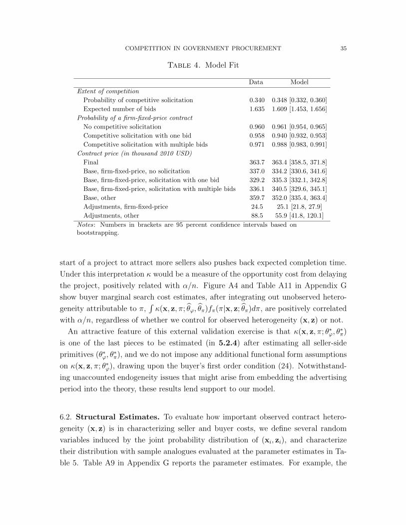
COMPETITION IN GOVERNMENT PROCUREMENT 35
Table 4. Model Fit
Data Model
Extent of competition
Probability of competitive solicitation 0.340 0.348 [0.332, 0.360]
Expected number of bids 1.635 1.609 [1.453, 1.656]
Probability of a firm-fixed-price contract
No competitive solicitation 0.960 0.961 [0.954, 0.965]
Competitive solicitation with one bid 0.958 0.940 [0.932, 0.953]
Competitive solicitation with multiple bids 0.971 0.988 [0.983, 0.991]
Contract price (in thousand 2010 USD)
Final 363.7 363.4 [358.5, 371.8]
Base, firm-fixed-price, no solicitation 337.0 334.2 [330.6, 341.6]
Base, firm-fixed-price, solicitation with one bid 329.2 335.3 [332.1, 342.8]
Base, firm-fixed-price, solicitation with multiple bids 336.1 340.5 [329.6, 345.1]
Base, other 359.7 352.0 [335.4, 363.4]
Adjustments, firm-fixed-price 24.5 25.1 [21.8, 27.9]
Adjustments, other 88.5 55.9 [41.8, 120.1]
Notes: Numbers in brackets are 95 percent confidence intervals based onbootstrapping.
start of a project to attract more sellers also pushes back expected completion time.
Under this interpretation κ would be a measure of the opportunity cost from delaying
the project, positively related with α/n. Figure A4 and Table A11 in Appendix G
show buyer marginal search cost estimates, after integrating out unobserved hetero-
geneity attributable to π,∫κ(x, z, π; θϕ, θπ)fπ(π|x, z; θπ)dπ, are positively correlated
with α/n, regardless of whether we control for observed heterogeneity (x, z) or not.
An attractive feature of this external validation exercise is that κ(x, z, π; θ∗ϕ, θ∗π)
is one of the last pieces to be estimated (in 5.2.4) after estimating all seller-side
primitives (θ∗ϕ, θ∗π), and we do not impose any additional functional form assumptions
on κ(x, z, π; θ∗ϕ), drawing upon the buyer’s first order condition (24). Notwithstand-
ing unaccounted endogeneity issues that might arise from embedding the advertising
period into the theory, these results lend support to our model.
6.2. Structural Estimates. To evaluate how important observed contract hetero-
geneity (x, z) is in characterizing seller and buyer costs, we define several random
variables induced by the joint probability distribution of (xi, zi), and characterize
their distribution with sample analogues evaluated at the parameter estimates in Ta-
ble 5. Table A9 in Appendix G reports the parameter estimates. For example, the

36 KARAM KANG AND ROBERT A. MILLER
Table 5. Estimating the Role of Observed Heterogeneity
All contracts Mean differences:Mean Median SD Product Commercially
vs. services available vs. not
Fraction of low-cost sellers 0.940 0.963 0.065 0.097 0.031(0.004) (0.004) (0.004) (0.008) (0.006)
Project costs of low-cost sellers 360.87 244.69 141.81 -27.19 -11.23
(3.54) (4.78) (2.04) (6.80) (5.38)
Project cost difference 40.91 20.37 46.55 -2.02 19.24(30.63) (19.37) (32.27) (36.00) (38.55)
Maximal benefits of competition† 4.51 1.16 13.17 -6.61 -0.46(1.12) (0.72) (5.09) (2.56) (1.91)
Marginal search costs 1.70 0.56 4.65 -3.73 -0.32(0.53) (0.43) (1.20) (1.29) (0.77)
Solicitation costs 0.06 0.06 0.02 -0.01 0.003(0.14) (0.14) (0.07) (0.05) (0.03)
Conditional soliciting costs -0.01 -0.01 0.02 -0.01 0.01(0.06) (0.23) (0.14) (0.06) (0.03)
Notes: This table provides summary statistics of the distribution of the mean values of thefraction of low-cost sellers, sellers’ project costs, and the buyer’s search and solicitation costs,integrated over π and evaluated at each realization of (xi, zi) and the estimated parameters.It also provides the mean differences between contracts for products and those for services,as well as the differences in means between contracts for commercially available versus un-available products and services. All cost estimates are in thousand 2010 dollars. Numbers inparentheses are bootstrap standard errors. † See (34) for the definition.
expected project cost for a type k seller conditional on (x, z), integrated over π, is:37
Eπ(ck|x, z; θ∗ϕ, θ∗π) ≡
∫ck(x1, π; θ∗ϕ
)fπ(π|x, z; θ∗π)dπ.
In Table 5, the mean of low-cost sellers’ project costs is estimated by averaging
Eπ(c1|xi, zi; θϕ, θπ) over the sample i ∈ 1, . . . , I.38
In addition, we show how the estimated primitives vary with π in Figure 2. Panel
(A) of Figure 2 displays the estimated cumulative distribution function of π condi-
tional on whether the contract is competitively solicited or not, after integrating out
37To clarify which variable the expectation is taken over, we use the subscript notation right next tothe expectation operator. For example, Eπ(·) denotes the value of the term in parentheses integratedover the density of π.38Bootstrap standard errors in Table 5 indicate the mean project cost differences and the meansolicitation costs are imprecisely estimated, but bootstrap confidence intervals in Table 6 are fairlytight. This apparent discrepancy may be explained by (i) our relatively precise parameter estimatesof the π distribution and marginal search costs, key to the buyer’s trade-off for extra bids; (ii)high-cost contracts comprising only 4 percent of the sample, yet providing an important source ofvariation for identification and estimation.
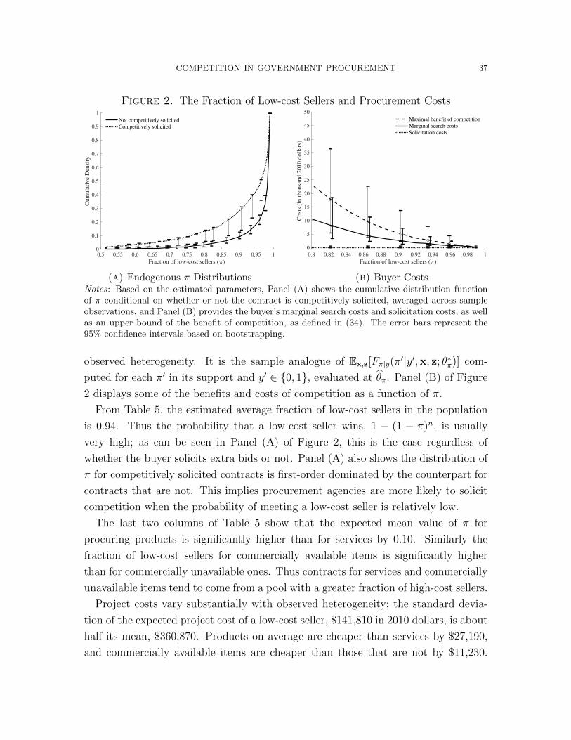
COMPETITION IN GOVERNMENT PROCUREMENT 37
Figure 2. The Fraction of Low-cost Sellers and Procurement Costs
0.5 0.55 0.6 0.65 0.7 0.75 0.8 0.85 0.9 0.95 1
Fraction of low-cost sellers ( )
0
0.1
0.2
0.3
0.4
0.5
0.6
0.7
0.8
0.9
1
Cu
mu
lati
ve
Den
sity
Not competitively solicited
Competitively solicited
(a) Endogenous π Distributions
0.8 0.82 0.84 0.86 0.88 0.9 0.92 0.94 0.96 0.98 1
Fraction of low-cost sellers ( )
0
5
10
15
20
25
30
35
40
45
50
Cost
s (i
n t
housa
nd 2
010 d
oll
ars)
Maximal benefit of competition
Marginal search costs
Solicitation costs
(b) Buyer CostsNotes: Based on the estimated parameters, Panel (A) shows the cumulative distribution functionof π conditional on whether or not the contract is competitively solicited, averaged across sampleobservations, and Panel (B) provides the buyer’s marginal search costs and solicitation costs, as wellas an upper bound of the benefit of competition, as defined in (34). The error bars represent the95% confidence intervals based on bootstrapping.
observed heterogeneity. It is the sample analogue of Ex,z[Fπ|y(π′|y′,x, z; θ∗π)] com-
puted for each π′ in its support and y′ ∈ 0, 1, evaluated at θπ. Panel (B) of Figure
2 displays some of the benefits and costs of competition as a function of π.
From Table 5, the estimated average fraction of low-cost sellers in the population
is 0.94. Thus the probability that a low-cost seller wins, 1 − (1 − π)n, is usually
very high; as can be seen in Panel (A) of Figure 2, this is the case regardless of
whether the buyer solicits extra bids or not. Panel (A) also shows the distribution of
π for competitively solicited contracts is first-order dominated by the counterpart for
contracts that are not. This implies procurement agencies are more likely to solicit
competition when the probability of meeting a low-cost seller is relatively low.
The last two columns of Table 5 show that the expected mean value of π for
procuring products is significantly higher than for services by 0.10. Similarly the
fraction of low-cost sellers for commercially available items is significantly higher
than for commercially unavailable ones. Thus contracts for services and commercially
unavailable items tend to come from a pool with a greater fraction of high-cost sellers.
Project costs vary substantially with observed heterogeneity; the standard devia-
tion of the expected project cost of a low-cost seller, $141,810 in 2010 dollars, is about
half its mean, $360,870. Products on average are cheaper than services by $27,190,
and commercially available items are cheaper than those that are not by $11,230.
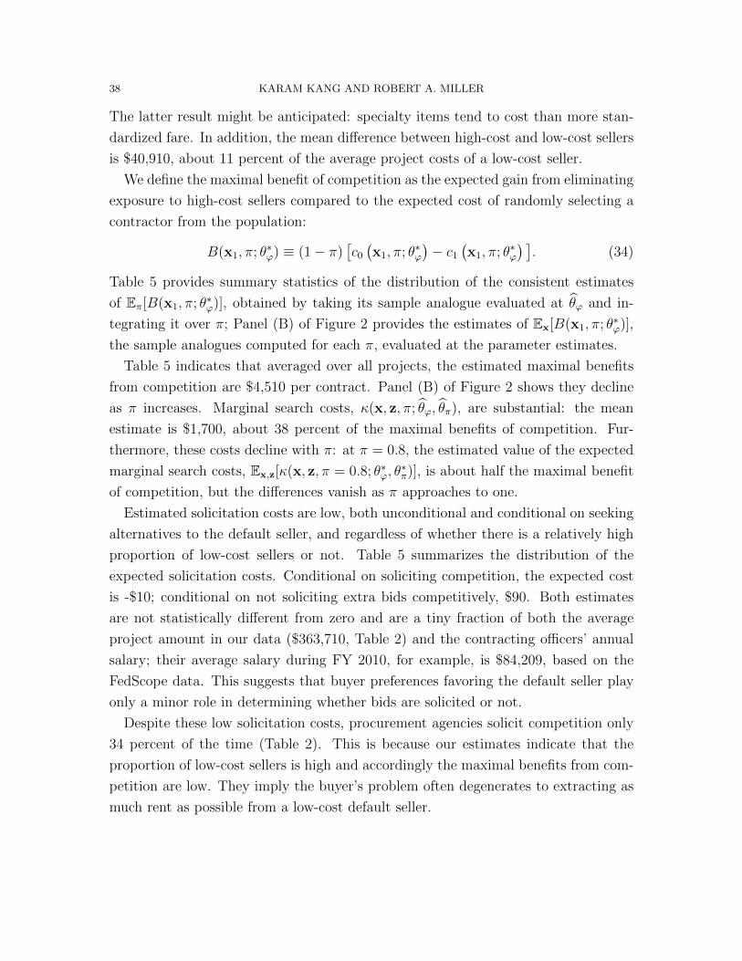
38 KARAM KANG AND ROBERT A. MILLER
The latter result might be anticipated: specialty items tend to cost than more stan-
dardized fare. In addition, the mean difference between high-cost and low-cost sellers
is $40,910, about 11 percent of the average project costs of a low-cost seller.
We define the maximal benefit of competition as the expected gain from eliminating
exposure to high-cost sellers compared to the expected cost of randomly selecting a
contractor from the population:
B(x1, π; θ∗ϕ) ≡ (1− π)[c0
(x1, π; θ∗ϕ
)− c1
(x1, π; θ∗ϕ
) ]. (34)
Table 5 provides summary statistics of the distribution of the consistent estimates
of Eπ[B(x1, π; θ∗ϕ)], obtained by taking its sample analogue evaluated at θϕ and in-
tegrating it over π; Panel (B) of Figure 2 provides the estimates of Ex[B(x1, π; θ∗ϕ)],
the sample analogues computed for each π, evaluated at the parameter estimates.
Table 5 indicates that averaged over all projects, the estimated maximal benefits
from competition are $4,510 per contract. Panel (B) of Figure 2 shows they decline
as π increases. Marginal search costs, κ(x, z, π; θϕ, θπ), are substantial: the mean
estimate is $1,700, about 38 percent of the maximal benefits of competition. Fur-
thermore, these costs decline with π: at π = 0.8, the estimated value of the expected
marginal search costs, Ex,z[κ(x, z, π = 0.8; θ∗ϕ, θ∗π)], is about half the maximal benefit
of competition, but the differences vanish as π approaches to one.
Estimated solicitation costs are low, both unconditional and conditional on seeking
alternatives to the default seller, and regardless of whether there is a relatively high
proportion of low-cost sellers or not. Table 5 summarizes the distribution of the
expected solicitation costs. Conditional on soliciting competition, the expected cost
is -$10; conditional on not soliciting extra bids competitively, $90. Both estimates
are not statistically different from zero and are a tiny fraction of both the average
project amount in our data ($363,710, Table 2) and the contracting officers’ annual
salary; their average salary during FY 2010, for example, is $84,209, based on the
FedScope data. This suggests that buyer preferences favoring the default seller play
only a minor role in determining whether bids are solicited or not.
Despite these low solicitation costs, procurement agencies solicit competition only
34 percent of the time (Table 2). This is because our estimates indicate that the
proportion of low-cost sellers is high and accordingly the maximal benefits from com-
petition are low. They imply the buyer’s problem often degenerates to extracting as
much rent as possible from a low-cost default seller.
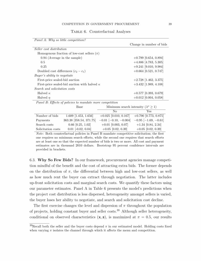
COMPETITION IN GOVERNMENT PROCUREMENT 39
Table 6. Counterfactual Analyses
Panel A: Why so little competition?
Change in number of bids
Seller cost distribution
Homogenous fraction of low-cost sellers (π)
0.94 (Average in the sample) +0.799 [0.654, 0.894]
0.5 +4.886 [4.783, 5.305]
0.25 +9.241 [9.010, 9.984]
Doubled cost differences (c2 − c1) +0.664 [0.521, 0.747]
Buyer’s ability to negotiate
First-price sealed-bid auction +2.728 [1.462, 3.375]
First-price sealed-bid auction with halved κ +3.432 [1.989, 4.108]
Search and solicitation costs
Halved κ +0.577 [0.393, 0.679]
Halved η +0.012 [0.004, 0.058]
Panel B: Effects of policies to mandate more competition
Base Minimum search intensity (λo ≥ 1)
No Yes
Number of bids 1.609 [1.453, 1.656] +0.025 [0.010, 0.167] +0.790 [0.773, 0.875]
Payments 363.38 [358.54, 371.75] −0.01 [−0.10, −0.004] −0.95 [−1.69, −0.61]
Search costs 0.66 [0.25, 1.02] +0.01 [0.003, 0.07] +1.34 [0.84, 2.34]
Solicitation costs 0.01 [-0.02, 0.04] +0.05 [0.02, 0.39] +0.05 [0.02, 0.39]
Note: Both counterfactual policies in Panel B mandate competitive solicitation; the firstone requires no minimum search efforts, while the second one requires that search effortsare at least one so that the expected number of bids is two or more. All cost and paymentestimates are in thousand 2010 dollars. Bootstrap 95 percent confidence intervals areprovided in brackets.
6.3. Why So Few Bids? In our framework, procurement agencies manage competi-
tion mindful of the benefit and the cost of attracting extra bids. The former depends
on the distribution of π, the differential between high and low-cost sellers, as well
as how much rent the buyer can extract through negotiation. The latter includes
up-front solicitation costs and marginal search costs. We quantify these factors using
our parameter estimates. Panel A in Table 6 presents the model’s predictions when
the project cost distribution is less dispersed, heterogeneity amongst sellers is varied,
the buyer loses her ability to negotiate, and search and solicitation cost decline.
The first exercise changes the level and dispersion of π throughout the population
of projects, holding constant buyer and seller costs.39 Although seller heterogeneity,
conditional on observed characteristics (x, z), is maximized at π = 0.5, our results
39Recall both the seller and the buyer costs depend π in our estimated model. Holding costs fixedwhen varying π isolates the channel through which it affects the menu and competition.
40 KARAM KANG AND ROBERT A. MILLER
show that as π declines, the number of expected bidders increases even beyond 9.2
extra bids at π = 0.25, before declining at values near zero. In addition, removing
all dispersion of π over the population, and fixing the proportion of low-cost sellers
for every project to Ex,z,π[πi; θπ] increases the expected number of extra bidders,
by 0.8. These findings show that the high average values of π and its dispersion
help explain why there are so few bids for government procurement projects in this
sector. Intuitively, when π is close to one, the buyer protects herself against a “lemon
default seller,” but when π is close to zero, she is “bargain hunting.” Our estimates
indicate the latter scenario generates more search in equilibrium than the former, yet
contacting officers are much more likely to find themselves in the former scenario.
In our framework the buyer is cast as an effective negotiator that squeezes the prof-
its of the high-cost seller to zero, and the profits of the low-cost seller to the amount
necessary to induce truth-telling in this private information environment. This ex-
plains why the buyer needs to attract fewer bids than what an auction framework
requires, to achieve the same outcome. To quantify the buyer’s power to extract rent
by limiting her discretion, we consider a first-price sealed-bid auction with a reserve
price of γ0.40 In this auction, the contract type is set to be firm-fixed-price: sellers bid
the base price, are liable for the initial project cost, and get reimbursed for uncertain
cost changes. The equilibrium for this auction consists of two base prices, p′′n and γ0,
where p′′n takes precedence over γ0 and p′′n is defined:41
p′′n ≡ γ1 +π(1− π)n−1
1− (1− π)n(γ0 − γ1) . (35)
Note that p′′n = γ0 when n = 1, decreasing in n to converge to γ1 as n → ∞. By
Corollary 3.1, he expected total payment in this auction, TFIC(n), is higher than its
negotiation counterpart, T (n). Under this scenario, if solicitation and marginal search
costs are held constant, it is optimal for the buyer to search more intensely, increasing
the expected number of sellers by 2.73. This reduces the estimated expected payment
by $10 per contract, a small and statistically insignificant amount.
We speculate that conducting a first-price sealed-bid auction might be simpler than
a negotiation process. Following that vein, consider a first-price sealed-bid auction
where buyer search is half as costly for auctions compared to negotiations. Panel A
of Table 6 shows that in such a scenario, the expected number of bids is 3.43 higher.
40Appendix F.2 describes how to implement this quantification exercise.41Lemma A4 in the Appendix shows these prices form the optimal menu when the buyer is con-strained to offer full insurance contracts. It is straightforward to establish, by a contradictionargument, that a first-price sealed bid scoring auction achieves these prices and allocation rule.

COMPETITION IN GOVERNMENT PROCUREMENT 41
With more than twice the bids, total search costs are higher in the auction, but only
a modest reduction in total payments is achieved, 0.25 percent or $895 per contract,
for the reasons we explain above. It is not obvious an auction format is preferable
even if attracting competitors is cheaper than in negotiations.
Turning to the buyer’s costs, the solicitation costs, η, do not play a very important
role in determining the optimal number of bids. Even if the value of η is halved, we
estimate the expected number of bids would only increase by 0.01. On the other hand
if marginal search costs, κ, are halved, we would expect 0.58 more bids. Although
these estimates imply that the elasticity of bids with respect to marginal search costs
is much greater than that with respect to solicitation costs, we cannot conclude that
it is more cost-effective to invest in reducing marginal search costs than solicitation
costs because on average κ is more than an order of magnitude greater that η.
6.4. Policies to Mandate Competition. To quantify the extent to which more
competition can reduce the amount of payments to contractors, we consider two
counterfactual policies. Both involve removing the buyer’s discretion to forego com-
petition and automatically award the project to a default seller. Thus the estimated
distribution of solicitation costs, Fη, is not used for these counterfactual exercises,
and since it is the final piece of the estimation procedure, our results on this segment
are robust to misspecification of the distribution.
Under one policy, competitive solicitation is mandatory for all projects, but buyers
have discretion in choosing their effort to attract more bids. The other policy requires
the minimum amount of search efforts is one, so that the buyer attracts a greater
number of bids than two in expectation.42 Panel B of Table 6 shows these two
policies would increase the average number of bids by 0.03 and 0.79, respectively, but
the expected amount of payments to contractors would only decline by $10 and $950
per contract, less than 0.3 percent of the average payment size per contract under the
current policy.43
These two alternative policies would decrease the size of the expected payments:
increasing competition makes the selection of a low-cost seller more likely, thus reduc-
ing the project costs. However, Table 6 shows that these cost savings are more than
42For these two policies, the equilibrium search efforts, or equivalently the equilibrium number ofbids, λo, are theoretically derived and calculated based on the estimates (Appendix F.3).43These findings are consistent with Coviello et al. (2018). Based on a regression discontinuity designusing data on public procurement in Italy, they show that increasing the buyer’s discretion does notworsen procurement outcomes, and may even improve them. Using the Nigerian Civil Service data,Rasul and Rogger (2018) find that increasing bureaucrats’ autonomy is positively associated withcompletion rates.

42 KARAM KANG AND ROBERT A. MILLER
offset by an increase in the search and competitive solicitation costs. To the extent
that the search costs reflect frictions in the market that are beyond the scope of a
single buyer’s responsibility (Kelman, 1990, 2005) and the costs of soliciting competi-
tive bids represent a legitimate social cost (for example due to higher noncontractible
quality of the default seller), both policies are suboptimal.
7. Conclusion
This paper is an empirical analysis of government procurement where procurement
agencies have discretion about the extent of competition and contract terms. Our
theory predicts that for any given number of bidders, procurement agencies can ex-
tract more rent from a winning seller when they negotiate, compared to running an
auction. The agencies’ ability to negotiate reduces their marginal value from promot-
ing competition and attracting more bids. For example, we estimate that stripping
the agencies of their discretion in designing and negotiating contracts would more
than double the average number of bids, but hardly reduce the size of the payment
to winning sellers. Allowing procurement agencies to exercise some discretion to use
their knowledge of the supply side can reduce procurement costs, even if they simul-
taneously engage in some rent-seeking behavior. Broadly speaking, our findings are
not very sensitive to the estimated costs of soliciting competition; agencies would,
however, increase their search intensity and enlarge the pool of sellers if there was
greater heterogeneity in the seller cost components. Our framework provides a tem-
plate for analyzing other procurement auctions that attract only a modest number of
bids.
References
An, Y. and X. Tang (2019). Specification and negotiation in incomplete contracts.
RAND Journal of Economics 50 (1), 57–92.
Arve, M. and D. Martimort (2016). Dynamic procurement under uncertainty: Op-
timal design and implications for incomplete contracts. American Economic Re-
view 106 (11), 3238–3274.
Athey, S., D. Coey, and J. Levin (2013). Set-asides and subsidies in auctions. Amer-
ican Economic Journal: Microeconomics 5 (1), 1–27.
Athey, S., J. Levin, and E. Seira (2011). Comparing open and sealed bid auctions:
Evidence from timber auctions. Quarterly Journal of Economics 126 (1), 207–257.
COMPETITION IN GOVERNMENT PROCUREMENT 43
Bajari, P., H. Hong, and S. P. Ryan (2010). Identification and estimation of a discrete
game of complete information. Econometrica 78 (5), 1529–1568.
Bajari, P. and A. Hortacsu (2003). The winner’s curse, reserve prices, and endogenous
entry: Empirical insights from ebay auctions. RAND Journal of Economics 34 (2),
329–355.
Bajari, P., S. Houghton, and S. Tadelis (2014). Bidding for incomplete contracts:
An empirical analysis of adaptation costs. American Economic Review 104 (4),
1288–1319.
Bajari, P., R. McMillan, and S. Tadelis (2008). Auctions versus negotiations in
procurement: An empirical analysis. Journal of Law, Economics, & Organiza-
tion 25 (2), 372–399.
Bajari, P. and S. Tadelis (2001). Incentives versus transaction costs: A theory of
procurement contracts. RAND Journal of Economics 32 (3), 387–407.
Bandiera, O., A. Prat, and T. Valletti (2009). Active and passive waste in government
spending: Evidence from a policy experiment. American Economic Review 99 (4),
1278–1308.
Barkley, A., J. R. Groeger, and R. A. Miller (2021). Bidding frictions in ascending
auctions. Journal of Econometrics 223 (2), 376–400.
Baron, D. P. and D. Besanko (1987). Monitoring, moral hazard, asymmetric infor-
mation, and risk sharing in procurement contracting. RAND Journal of Econom-
ics 18 (4), 509–532.
Bhattacharya, V. (forthcoming). An empirical model of R&D procurement contests:
An analysis of the DOD SBIR program. Econometrica.
Bulow, J. and P. Klemperer (2002). Prices and the winner’s curse. RAND Journal
of Economics 33 (1), 1–21.
Che, Y.-K. and I. Gale (2003). Optimal design of research contests. American Eco-
nomic Review 93 (3), 646–671.
Compiani, G., P. Haile, and M. Sant’Anna (2020). Common values, unobserved
heterogeneity, and endogenous entry in U.S. offshore oil lease auctions. Journal of
Political Economy 128 (10), 3872–3912.
Coviello, D., A. Guglielmo, and G. Spagnolo (2018). The effect of discretion on
procurement performance. Management Science 64 (2), 715–738.
Crocker, K. J. and K. J. Reynolds (1993). The efficiency of incomplete contracts:
An empirical analysis of air force engine procurement. RAND Journal of Econom-
ics 24 (1), 126–146.

44 KARAM KANG AND ROBERT A. MILLER
Decarolis, F. (2014). Awarding price, contract performance, and bids screening: Evi-
dence from procurement auctions. American Economic Journal: Applied Econom-
ics 6 (1), 108–132.
Decarolis, F., L. M. Giuffrida, E. Iossa, V. Mollisi, and G. Spagnolo (2020). Buyer
competence and procurement outcomes. Journal of Law, Economics, and Organi-
zation 36 (3), 537–597.
Fullerton, R. L. and R. P. McAfee (1999). Auctioning entry into tournaments. Journal
of Political Economy 107 (2), 573–605.
Gagnepain, P., M. Ivaldi, and D. Martimort (2013). The cost of contract renego-
tiation: Evidence from the local public sector. American Economic Review 103,
2352–2383.
Gayle, G.-L. and R. A. Miller (2015). Identifying and testing models of managerial
compensation. The Review of Economic Studies 82 (3), 1074–1118.
Guerre, E. and Y. Luo (2019). Nonparametric identification of first-price auction with
unobserved competition: A density discontinuity framework. mimeo.
Hendricks, K., J. Pinkse, and R. H. Porter (2003). Empirical implications of equilib-
rium bidding in first-price, symmetric, common value auctions. Review of Economic
Studies 70 (1), 115–145.
Kelman, S. (1990). Procurement and Public Management: The Fear of Discretion
and the Quality of Government Performance. The AEI Press.
Kelman, S. (2005). Unleashing Change: A Study of Organizational Renewal in Gov-
ernment. Brookings Institution.
Krasnokutskaya, E. (2011). Identification and estimation in procurement auctions
under unobserved auction heterogeneity. Review of Economic Studies 78 (1), 293–
327.
Krasnokutskaya, E. and K. Seim (2011). Bid preference programs and participation
in highway procurement auctions. American Economic Review 101, 2653–2686.
Laffont, J.-J. and J.-C. Rochet (1998). Regulation of a risk averse firm. Games and
Economic Behavior 35 (3), 149–173.
Laffont, J.-J. and J. Tirole (1987). Auctioning incentive contracts. Journal of Political
Economy 95, 921–937.
Laffont, J.-J. and J. Tirole (1993). A Theory of Incentives in Procurement and Reg-
ulation. Cambridge, Mass.: MIT Press.
Lewis, G. and P. Bajari (2011). Procurement contracting with time incentives: Theory
and evidence. Quarterly Journal of Economics 126, 1173–1211.

COMPETITION IN GOVERNMENT PROCUREMENT 45
Lewis, G. and P. Bajari (2014). Moral hazard, incentive contracts and risk: Evidence
from procurement. Review of Economic Studies 81, 1201–1228.
Li, T. (2005). Econometrics of first-price auctions with entry and binding reservation
prices. Journal of Econometrics 126, 173–200.
Li, T. and X. Zheng (2009). Entry and competition effects in first-price auctions: The-
ory and evidence from procurement auctions. Review of Economic Studies 76 (4),
1397–1429.
Liebman, J. B. and N. Mahoney (2017). Do expiring budgets lead to wasteful
year-end spending? Evidence from federal procurement. American Economic Re-
view 107 (11), 3510–49.
MacKay, A. (forthcoming). Contract duration and the costs of market transactions.
American Economic Journal: Microeconomics .
Manelli, A. M. and D. R. Vincent (1995). Optimal procurement mechanisms. Econo-
metrica 63 (3), 591–620.
McAfee, R. P. and J. McMillan (1987). Competition for agency contracts. RAND
Journal of Economics 18 (2), 296–307.
Perrigne, I. and Q. Vuong (2011). Nonparametric identification of a contract model
with adverse selection and moral hazard. Econometrica 79, 1499–1539.
Pinkse, J. and G. Tan (2005). The affiliation effect in first-price auctions. Economet-
rica 73 (1), 263–277.
Porter, R. H. and J. D. Zona (1993). Detection of bid rigging in procurement auctions.
Journal of Political Economy 101 (3), 518–538.
Rasul, I. and D. Rogger (2018). Management of bureaucrats and public service deliv-
ery: Evidence from the Nigerian civil service. Economic Journal 128 (608), 413–446.
Riordan, M. H. and D. E. Sappington (1987). Awarding monopoly franchises. Amer-
ican Economic Review 77 (3), 375–387.
Taylor, C. R. (1995). Digging for golden carrots: An analysis of research tournaments.
American Economic Review 85 (4), 872–890.
Warren, P. L. (2014). Contracting officer workload, incomplete contracting, and
contractual terms. RAND Journal of Economics 45 (2), 395–421.
46 KARAM KANG AND ROBERT A. MILLER
Appendix A. Constructing the Dataset
A.1. Definition of variables.
A.1.1. Contract price: Base and final. The FPDS (Federal Procurement Data Sys-
tem) database provides three variables on the price of each contract action: (i) “base
and all options value,” the total contract value including all options including those
not yet exercised; (ii) “base and exercised options value,” the contract value for the
base contract and any options that have been exercised; (iii) “action obligation,” the
amount that is obligated or de-obligated by the action. We define that the final price
is the sum of all obligated amounts related to the contract; the base price is defined
as the base and exercised options value as of the date that the contract was signed.
A.1.2. Contract duration: Base and final. The FPDS database provides four vari-
ables on the dates related to each contract action: (1) “date signed,” the date that
the action was signed; (ii) “effective date,” the date that the parties agree will be
the starting date for the contract requirements; (iii) “current completion date,” the
completion date of the base contract plus options that have been exercised; (iv) “ul-
timate completion date,” the estimated or scheduled completion date including the
base contract and all exercised and unexercised options. We define that the start date
is the latter date of the date signed and the effective date in the initial entry; the base
duration is the difference between the current completion date in the initial entry and
the start date; the final duration is the difference between the current completion date
as in the last entry and the start date. Note that we observe the expected completion
date as in the last entry of a contract, not its actual completion date. Because further
entries might occur after we retrieved the data from the FPDS (July 2018), we focus
on contracts whose current completion date in the last contract entry lies before the
end of FY 2017.
A.1.3. Price and duration adjustments. All contract actions, including the initial
agreement and the subsequent adjustments, are recorded as entries in the FPDS
database. Based on these entries, we construct the history of price and duration
adjustments. Each contract action entry specifies the reason for the action, with
the variable called “reason for modification.” The variable value can take one of the
reasons shown in Table A1, grouped into three categories: work changes, exercise of
options and funding, and administrative actions. Using the “date signed” variable,
we obtain the chronological order of all entries, and track the price and the duration
adjustments based on the “action obligation amount” and the “current completion

COMPETITION IN GOVERNMENT PROCUREMENT 47
Table A1. Price and Duration Adjustments
Any Price Duration(%) ($K, 2010 USD) (days)
Mean SD Mean SD
Work changes
Additional work (new agreement) 1.69 116.56 224.68 114.09 177.01
Supplemental agreement for work within scope 9.65 39.66 118.80 113.48 208.78
Change order 5.51 27.40 119.50 89.31 252.40
Definitize change order or letter contract 0.27 153.85 196.82 41.68 86.18
Termination for convenience 0.72 -154.71 151.29 -9.72 110.62
Termination for cause 0.04 -49.02 58.80 0.00 0.00
Termination for default 0.04 -228.81 73.11 0.00 0.00
Legal contract cancellation 0.21 -218.12 172.07 -29.13 81.35
Options and funding
Exercise of an option 6.49 261.60 224.88 450.57 401.21
Funding only 9.98 58.91 181.91 136.27 293.11
Administrative actions
Close-out 8.97 -20.65 79.43 83.19 304.49
Vendor information change 0.33 2.17 10.63 21.64 96.40
Other administrative action 28.23 -0.36 59.10 66.43 220.94
Transfer or non-novated merger & acquisition 0.16 0.00 0.00 89.18 354.73
Novation agreement 0.37 2.55 12.99 8.92 79.93
Note: All contracts in the final sample are included. Column entitled as “Any” provides thefraction of the contracts with entries associated with a given reason. Conditional on havingthe respective entries, the average and standard deviation of the price adjustments (in thousanddollars, CPI-adjusted to 2010) and the duration adjustments (in days) are provided.
date” variables. Table A1 provides summary statistics of price and duration adjust-
ments for each reason.
After the initial agreement on a contract, additional contract actions may be taken,
relating to contract cost, schedule, fee, terms and conditions, and personnel. The need
for such an action may arise due to changes in technologies, funding, and mission re-
quirements. An “administrative” action applies when the substantive rights of either
of the contracting parties are not affected by the action. An example of such an action
is “close-out,” which occurs when a contract has met all the terms of a contract and
final payment has been made (FAR 4.804). Among the non-administrative contract
actions, some (specifically, “additional work (new agreement)” and “supplemental
agreement for work within scope”) require both the contractor’s and the contracting
officer’s signatures. Others do not require the contractor’s signature because they
are based on numerous clauses within the contract. The text for such clauses to be
48 KARAM KANG AND ROBERT A. MILLER
inserted in the contract, for example for change order, options, incremental funding,
or termination, can be found in FAR 52.
A.1.4. Extent of competition. A contract in the category of set-aside for small busi-
ness in Table 1 satisfies any of the following two conditions: (i) the “type of set aside”
variable in the FPDS dataset takes a value other than “none”; or (ii) the “reason not
competed” takes a value related to small business programs (“8AN,” “HZS,”“NZS,”
“SBA,” and “BI”). For a contract to be labeled as no competition by regulation, its
“reason not competed” variable must take “IA” (international agreement), “OTH”
(authorized by statute), or “UT” (a regulated utility). If a contract doesn’t belong to
either of the above two categories and its “extent competed” variable takes either “A:
Full and open competition” or “F: Competed under Simplified Acquisition Procedure
(SAP),” it belongs to full and open competition. Those satisfying none of the above
criteria fall into the category of no competition by discretion.
Note that in determining the four categories of the extent of competition, we do
not use the “number of offers received” variable. All of the contracts that were not
competed by regulation (3,376 contracts) or discretion (6,182 contracts) in Table 1,
except 43 contracts and 1 contract respectively, received a single offer. This may re-
flect that limiting competition does not necessarily mean that only a single contractor
is considered. However, in our final sample of the 6,981 contracts, all contracts that
are categorized as not competed (by discretion) received a single offer.
In Panel B of Table 1, there are five categories of solicitation procedures, and these
categories are directly from the FPDS variable entitled, “solicitation procedures.”
The procedures described in the variable include:“Negotiated proposal/quote”, “Sim-
plified acquisition,” “No Solicitation (Only One Source),” as well as various other
procedures such as “Sealed bid,” “Two step,” “Architect-Engineer,” “Basic research”
and “Multiple award fair opportunity.”
A.1.5. Contract type. The FPDS dataset has the “type of contract” variable, and
there are 16 different contract type codes for the variable, spanning from “Firm
Fixed Price,” “Fixed Price Incentive”, “Fixed Price Award Fee,” “Cost Plus Fixed
Fee,” “Cost Plus Incentive Fee,” to “Time and Materials,” and “Labor hours.” All
contract types are defined in FAR 16. A vast majority of the contracts in our final
sample (6,717 out of 6,981) are “Firm Fixed Price,” and the rest are mostly (212 out
of 264) cost-plus contracts.
COMPETITION IN GOVERNMENT PROCUREMENT 49
A.1.6. Project attributes. We construct the commercial availability variable based
on two FPDS variables, “commercial item acquisition procedures” and “information
technology commercial item category.” The former designates whether the solicitation
used the commercial item acquisition procedures. The latter is for computer hardware
or services contracted or funded by the Department of Defense, and represents the
commercial nature of the products or services. We define that the products or services
are commercial available if the “commercial item acquisition procedures” variable
is “Commercial Item” or the “information technology commercial item category”
variable is “Commercial Available,” “Other Commercial Item,” “Non-developmental
Item,” or “Commercial Service.”
The FPDS dataset has the “award type” variable, which can take four values:
“Definitive Contract,” “Purchase Order,” “Delivery Order,” and “BPA Call.” Our
study focuses on the first two types, and we construct a dummy variable indicating
that a contract is a definitive contract.
Using on the “State: Place of Performance” and “Congressional District: Place
of Performance” variables in the FPDS dataset, we identify the state and the Con-
gressional district of the location where a contract is performed. We obtain the
Congressional Committee assignment data, as collected by Charles Stewart III and
Jonathan Woon: “Congressional Committees, Modern Standing Committees, 103rd-
115th Congresses.” The Appropriations/Budget committee variable indicates that
the place of performance was represented, at the time of the signing the contract,
by House Speaker, majority/minority leaders and whips, and chairmen or ranking
members of the Committees on the Budget, Appropriations, and Ways and Means.
The “Congressional District: Place of Performance” variable is not always available,
especially for those in the FPDS dataset before 2007. For such contracts, we rely on
the state information only, which is always available.
A.1.7. Agency attributes. By combining the FedScope Employment Cube with the
FPDS data, we obtain the number and the government experience of the contracting
officers hired by a procurement agency. For each agency, the FedScope data provides
the number of employees by age, education, length of service, occupation, and pay
plan/grade. The occupation code for contracting officers is 1102, and we obtain the
number of all contracting officers in the agency and the numbers of such officers with
at least 5 years of government service for each fiscal year. We then merge the data with
the FPDS data, using the name of the government agency. Out of 235 agencies in the
FPDS dataset, 196 are well-matched by the name, but the match for the rest is not
50 KARAM KANG AND ROBERT A. MILLER
clear. Given this, we use a larger unit of the government agency, or a parent agency,
to merge the two datasets (69 parent agencies, such as the Department of Agriculture,
the Department of Commerce, etc.), as opposed to a smaller unit (for example, Food
Safety and Inspection Service, US Census Bureau, etc.). Given the agency-year-level
data, we construct the contracting officers with 5+ years and workload variables.
A.1.8. Measures of potential competition. We construct two measures of potential
competition, the number of past winners and the number of establishments. First,
for a given contract, we look at all contracts in the FPDS dataset that were signed
within three years and have the same values of Product and Service code, commercial
availability, contract instrument (definitive contract or purchase order), state of the
project location, and whether or not the Department of Defense is the procurement
agency. We then count the number of unique contractors who won these contracts,
based on the “Parent DUNS Number” variable, which is the identifier of the parent
company of the winner. Second, based on the “NAICS” variable, which designates
the principal North American Industry Classification System (NAICS) code for a
contract, and the “State: Place of Performance” variable, we merge our dataset with
the County Business Patterns dataset, which provides the number of establishments
by industry, state, and year, to construct the number of establishments variable.
A.1.9. Advertisement Period and Contract Types in Solicitations. To obtain informa-
tion on the procurement agency’s actions to advertise and publicize solicitations, we
combine the FPDS dataset with the information manually obtained from the federal
business opportunity website (www.fbo.gov). This website provides all public notices
regarding federal contract opportunities. To identify a public notice associated with
a contract in the FPDS dataset, we use the “solicitation identifier” variable. The
contracting officers are not required to report the solicitation identifier to the FPDS,
and only 712 contracts in our sample (10 percent) have such information. Among
them, we locate public notices for 394 contracts, and obtain the following: (i) the type
as specified in the notice (pre-solicitation, sources sought, draft solicitation, request
for information, request for proposal/quote, synopsis/solicitation, justification and
approval, special notice, award, and cancellation); (ii) the date on which the notice
was posted; (iii) the date by which a response by a contractor is requested. Whenever
available, we obtain the solicitation and the justification and approval documents.
Figure A1 provides an excerpt of a webpage of a public notice for a solicitation. On
the left panel, it provides the list of all public notices of the same strand, including the

COMPETITION IN GOVERNMENT PROCUREMENT 51
Figure A1. An Excerpt of a Public Notice on FBO.GOV
Notes: This is a screenshot of a part of a webpage of a public notice for solicitation VA11814R0665from www.fbo.gov, retrieved in August 2018.
pre-solicitation notice posted on September 15, 2014. In the middle panel, it specifies
that the notice type as “solicitation,” and a brief synopsis follows. On the right panel,
there are links to the attached documents, followed by the information on dates: this
notice was posted on September 23 and the response due date is September 26. The
advertisement period in this case is 12 days (from September 15 to 26).
A.2. Sample Selection. There are 41,189 IT and telecommunications contracts
with specified terms and conditions (definitive contracts or purchase orders) that
were initiated in FY 2004–2015. Panel A of Table A2 shows summary statistics of
the 17,123 contracts of Table 1 that satisfy all six sample selection criteria of Section
2.1, as well as those that do not meet each criterion, in the rows (A-1) to (A-6). Some
contracts fail on multiple criteria. We sequentially drop observations, implying the
sum of observations in rows (A-1) to (A-6) equals 41,189−17,123.

52 KARAM KANG AND ROBERT A. MILLER
Table A2. Sample Selection
Observations Final price ($K, 2010)Num. Frac. (%) Mean SD
Panel A: All IT/telecommunications 41,189 100.0 3,028.49 33,243.8
Sample used in Table 1 17,123 41.6 366.87 246.74
Out of sample due to:
(A-1) Base maximal price ≥ $1M (real) 9,188 22.3 11,886.65 68,602.3
(A-2) Base price ≤ $150K (nominal) 5,474 13.3 634.48 15,239.2
(A-3) Base duration < 30 or > 400 days 7,385 17.9 463.42 2,043.3
(A-4) Ended after the end of FY2017 228 0.6 2,084.9 13,680.4
(A-5) Performed outside of the U.S. 1,071 2.6 406.86 516.03
(A-6) Missing or inconsistent information† 720 1.8 1,996.1 2,924.8
Panel B: Sample used in Table 1 17,123 100.0 366.87 246.74
Final sample
Fully competed, negotiated 2,375 13.9 357.49 237.23
Not competed by discretion, negotiated 4,606 26.9 366.91 230.72
Out of sample due to:
(B-1) Not competed by rules 5,910 34.5 389.06 272.06
(B-2) Fully competed, other procedures 2,655 15.5 343.31 232.71
(B-3) Not competed by discretion, other proc. 1,577 9.2 337.36 220.48
Note: This table provides summary statistics of the final price of the contracts in the data,focusing on the IT and telecommunications contracts that initiated in FY 2004–2015, by thesample selection criteria discussed in Section 2.1 (Panel A) and Section 2.2 (Panel B). † Wedefine price or duration information is inconsistent when (i) the final delay of the contract isgreater than twenty times of the base duration (84 contracts); (ii) the final contract price islarger than three times of the base maximal price (524 contracts).
Panel B of Table A2 focuses on the sample used in Table 1, and presents summary
statistics of the final sample and the remainders. In addition to the six criteria
mentioned above, the contracts in the final sample satisfy two conditions: first, they
were either fully competed or not competitively solicited for discretionary reasons;
second, the contract terms were negotiated. The former rules out the 5,910 contracts,
those in Row (B-1), which were not solicited by regulation or were set-aside for small
business. The latter excludes the 2,655 contracts of the “full and open competition”
category, those in Row (B-2), and the 1,577 contracts of the “no competition by
discretion” category, those displayed in Row (B-3).
Appendix B. Further Evidence on the Assumptions
B.1. Competition and Winning History. Table A3 presents the summary sta-
tistics of our sample by the seller’s history of winning contracts and three industries
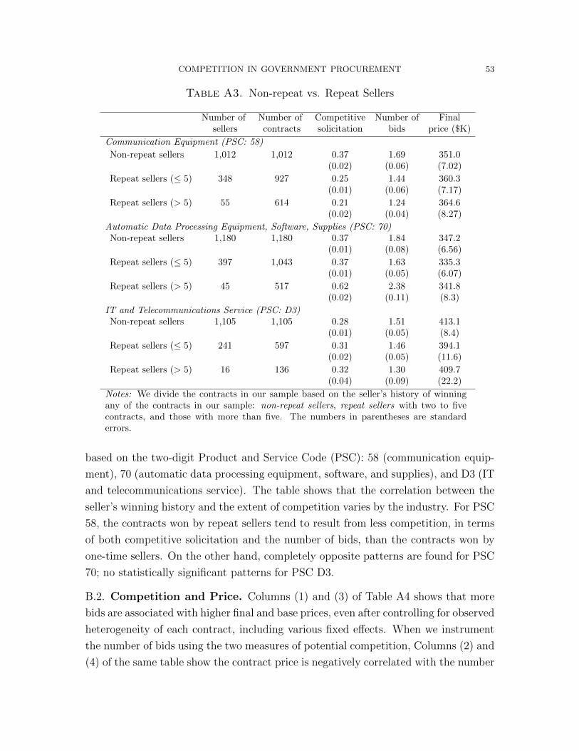
COMPETITION IN GOVERNMENT PROCUREMENT 53
Table A3. Non-repeat vs. Repeat Sellers
Number of Number of Competitive Number of Finalsellers contracts solicitation bids price ($K)
Communication Equipment (PSC: 58)
Non-repeat sellers 1,012 1,012 0.37 1.69 351.0(0.02) (0.06) (7.02)
Repeat sellers (≤ 5) 348 927 0.25 1.44 360.3(0.01) (0.06) (7.17)
Repeat sellers (> 5) 55 614 0.21 1.24 364.6(0.02) (0.04) (8.27)
Automatic Data Processing Equipment, Software, Supplies (PSC: 70)Non-repeat sellers 1,180 1,180 0.37 1.84 347.2
(0.01) (0.08) (6.56)
Repeat sellers (≤ 5) 397 1,043 0.37 1.63 335.3(0.01) (0.05) (6.07)
Repeat sellers (> 5) 45 517 0.62 2.38 341.8(0.02) (0.11) (8.3)
IT and Telecommunications Service (PSC: D3)Non-repeat sellers 1,105 1,105 0.28 1.51 413.1
(0.01) (0.05) (8.4)
Repeat sellers (≤ 5) 241 597 0.31 1.46 394.1(0.02) (0.05) (11.6)
Repeat sellers (> 5) 16 136 0.32 1.30 409.7(0.04) (0.09) (22.2)
Notes: We divide the contracts in our sample based on the seller’s history of winningany of the contracts in our sample: non-repeat sellers, repeat sellers with two to fivecontracts, and those with more than five. The numbers in parentheses are standarderrors.
based on the two-digit Product and Service Code (PSC): 58 (communication equip-
ment), 70 (automatic data processing equipment, software, and supplies), and D3 (IT
and telecommunications service). The table shows that the correlation between the
seller’s winning history and the extent of competition varies by the industry. For PSC
58, the contracts won by repeat sellers tend to result from less competition, in terms
of both competitive solicitation and the number of bids, than the contracts won by
one-time sellers. On the other hand, completely opposite patterns are found for PSC
70; no statistically significant patterns for PSC D3.
B.2. Competition and Price. Columns (1) and (3) of Table A4 shows that more
bids are associated with higher final and base prices, even after controlling for observed
heterogeneity of each contract, including various fixed effects. When we instrument
the number of bids using the two measures of potential competition, Columns (2) and
(4) of the same table show the contract price is negatively correlated with the number
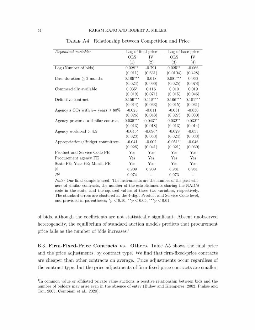
54 KARAM KANG AND ROBERT A. MILLER
Table A4. Relationship between Competition and Price
Dependent variable: Log of final price Log of base price
OLS IV OLS IV(1) (2) (3) (4)
Log (Number of bids) 0.028∗∗ -0.791 0.025∗∗ -0.066(0.011) (0.631) (0.0104) (0.428)
Base duration ≥ 3 months 0.109∗∗∗ -0.018 0.081∗∗∗ 0.066(0.024) (0.096) (0.025) (0.078)
Commercially available 0.035∗ 0.116 0.010 0.019(0.019) (0.071) (0.015) (0.046)
Definitive contract 0.159∗∗∗ 0.118∗∗∗ 0.106∗∗∗ 0.101∗∗∗
(0.014) (0.033) (0.015) (0.031)
Agency’s COs with 5+ years ≥ 80% -0.025 -0.011 -0.031 -0.030(0.026) (0.043) (0.027) (0.030)
Agency procured a similar contract 0.035∗∗∗ 0.043∗∗ 0.032∗∗ 0.032∗∗
(0.013) (0.018) (0.013) (0.014)
Agency workload > 4.5 -0.045∗ -0.096∗ -0.029 -0.035(0.023) (0.053) (0.024) (0.033)
Appropriations/Budget committees -0.041 -0.002 -0.051∗∗ -0.046(0.026) (0.041) (0.021) (0.030)
Product and Service Code FE Yes Yes Yes Yes
Procurement agency FE Yes Yes Yes Yes
State FE; Year FE; Month FE Yes Yes Yes Yes
N 6,909 6,909 6,981 6,981
R2 0.074 - 0.073 -
Note: Our final sample is used. The instruments are the number of the past win-ners of similar contracts, the number of the establishments sharing the NAICScode in the state, and the squared values of these two variables, respectively.The standard errors are clustered at the 4-digit Product and Service Code level,and provided in parentheses; ∗p < 0.10, ∗∗p < 0.05, ∗∗∗p < 0.01.
of bids, although the coefficients are not statistically significant. Absent unobserved
heterogeneity, the equilibrium of standard auction models predicts that procurement
price falls as the number of bids increases.1
B.3. Firm-Fixed-Price Contracts vs. Others. Table A5 shows the final price
and the price adjustments, by contract type. We find that firm-fixed-price contracts
are cheaper than other contracts on average. Price adjustments occur regardless of
the contract type, but the price adjustments of firm-fixed-price contracts are smaller,
1In common value or affiliated private value auctions, a positive relationship between bids and thenumber of bidders may arise even in the absence of entry (Bulow and Klemperer, 2002; Pinkse andTan, 2005; Compiani et al., 2020).
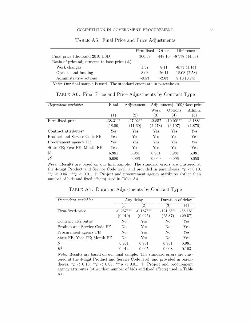
COMPETITION IN GOVERNMENT PROCUREMENT 55
Table A5. Final Price and Price Adjustments
Firm fixed Other Difference
Final price (thousand 2010 USD) 360.39 448.16 -87.78 (14.58)
Ratio of price adjustments to base price (%)
Work changes 1.37 8.11 -6.73 (1.14)
Options and funding 8.03 26.11 -18.08 (2.58)
Administrative actions -0.53 -2.63 2.10 (0.74)
Note: Our final sample is used. The standard errors are in parentheses.
Table A6. Final Price and Price Adjustments by Contract Type
Dependent variable: Final Adjustment |Adjustment|×100/Base price
Work Options Admin.(1) (2) (3) (4) (5)
Firm-fixed-price -38.31∗∗ -27.02∗∗ -2.857 -10.00∗∗∗ -3.188∗
(18.50) (11.69) (2.278) (3.197) (1.870)
Contract attributes† Yes Yes Yes Yes Yes
Product and Service Code FE Yes Yes Yes Yes Yes
Procurement agency FE Yes Yes Yes Yes Yes
State FE; Year FE; Month FE Yes Yes Yes Yes Yes
N 6,981 6,981 6,981 6,981 6,981
R2 0.080 0.096 0.060 0.096 0.050
Note: Results are based on our final sample. The standard errors are clustered atthe 4-digit Product and Service Code level, and provided in parentheses; ∗p < 0.10,∗∗p < 0.05, ∗∗∗p < 0.01. †: Project and procurement agency attributes (other thannumber of bids and fixed effects) used in Table A4.
Table A7. Duration Adjustments by Contract Type
Dependent variable: Any delay Duration of delay
(1) (2) (3) (4)
Firm-fixed-price -0.267∗∗∗ -0.187∗∗∗ -121.6∗∗∗ -58.16∗
(0.019) (0.025) (25.87) (29.57)
Contract attributes† No Yes No Yes
Product and Service Code FE No Yes No Yes
Procurement agency FE No Yes No Yes
State FE; Year FE; Month FE No Yes No Yes
N 6,981 6,981 6,981 6,981
R2 0.014 0.095 0.008 0.103
Note: Results are based on our final sample. The standard errors are clus-tered at the 4-digit Product and Service Code level, and provided in paren-theses; ∗p < 0.10, ∗∗p < 0.05, ∗∗∗p < 0.01. †: Project and procurementagency attributes (other than number of bids and fixed effects) used in TableA4.

56 KARAM KANG AND ROBERT A. MILLER
controlling for the base price, than those of other contracts. Columns (1) and (2) of
Table A6 show these patterns persist even after controlling for contract attributes.
Columns (3)–(5) of Table A6 show that price adjustments are less volatile for firm-
fixed-price contracts than other contracts. The dependent variables are the ratio
of the absolute value of the price adjustments, due to each of the three categories
respectively, to the base price; hence, the larger the ratio is, the more volatile the
price adjustments are. Column (4) shows that price adjustments associated with
exercising options or funding issues tend to be 10 percent lower than the base price.
Lastly, Table A7 show that firm-fixed-price contracts are less likely to have delays,
and conditional on having delays, the length is shorter, with or without controlling
for contract attributes.
B.4. Relationship between Price and Duration Adjustments. Column (1) of
Table A8 shows that price adjustments and delays are positively correlated. Con-
tracts seemingly reward delays, at odds with time incentive contracts induced by
moral hazard (Lewis and Bajari, 2011, 2014). This pattern may be driven by the
contractual agreement to fully or partially “reimburse” project cost changes under
various circumstances to manage the risk faced by the contractor. The financial and
accounting records of the contractor, as well as the cost control systems, are reviewed
by a government auditing agency to verify the claimed costs (FAR 42.101). Notably,
this positive correlation is pronounced for the adjustments that are likely to involve
cost changes, as shown in Columns (2)–(3), while it is reversed for the administra-
tive adjustments. This illustrates the importance of decomposing price and duration
adjustments for structural analysis.
Appendix C. Deriving the Optimal Contract Menu
Given a menu pjn, qjn (s)Jj=0 ≡ J we say individual rationality for a type k seller,
denoted by IRk, is satisfied if and only if:
maxj∈J
pjn − γk +
∫ψ[qjn (s)− c (s)]fk(s)ds
≡ max
j∈Jωjk ≡ ωk ≥ 0, (A.1)
where ωjk is the expected utility to a type k from winning the procurement by choosing
pjn, qjn (s) from the menu. We say IRk binds if ωk = 0. Without loss of generality
we ignore contracts that neither seller type choose in equilibrium. In a pooling menu
both seller types maximize their respective expected utilities by choosing all the
contracts on the menu with positive probability, and it is straightforward to establish
that the optimal pooling menu from the buyer’s perspective is one full insurance
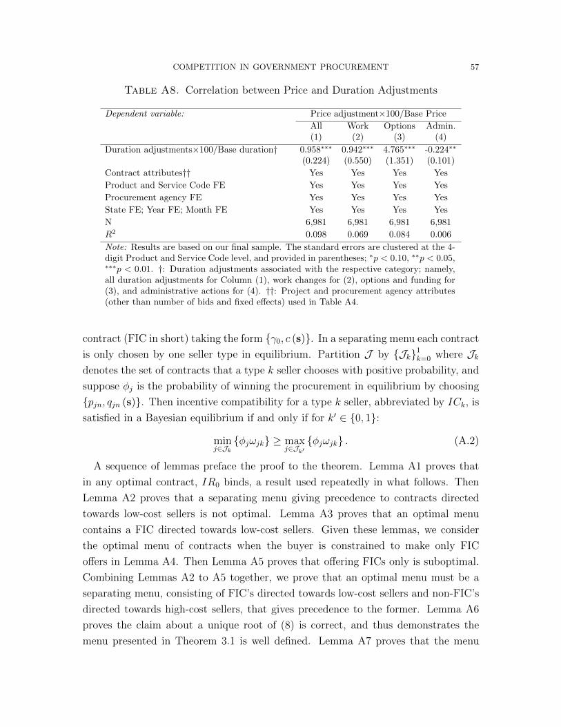
COMPETITION IN GOVERNMENT PROCUREMENT 57
Table A8. Correlation between Price and Duration Adjustments
Dependent variable: Price adjustment×100/Base Price
All Work Options Admin.(1) (2) (3) (4)
Duration adjustments×100/Base duration† 0.958∗∗∗ 0.942∗∗∗ 4.765∗∗∗ -0.224∗∗
(0.224) (0.550) (1.351) (0.101)
Contract attributes†† Yes Yes Yes Yes
Product and Service Code FE Yes Yes Yes Yes
Procurement agency FE Yes Yes Yes Yes
State FE; Year FE; Month FE Yes Yes Yes Yes
N 6,981 6,981 6,981 6,981
R2 0.098 0.069 0.084 0.006
Note: Results are based on our final sample. The standard errors are clustered at the 4-digit Product and Service Code level, and provided in parentheses; ∗p < 0.10, ∗∗p < 0.05,∗∗∗p < 0.01. †: Duration adjustments associated with the respective category; namely,all duration adjustments for Column (1), work changes for (2), options and funding for(3), and administrative actions for (4). ††: Project and procurement agency attributes(other than number of bids and fixed effects) used in Table A4.
contract (FIC in short) taking the form γ0, c (s). In a separating menu each contract
is only chosen by one seller type in equilibrium. Partition J by Jk1k=0 where Jk
denotes the set of contracts that a type k seller chooses with positive probability, and
suppose φj is the probability of winning the procurement in equilibrium by choosing
pjn, qjn (s). Then incentive compatibility for a type k seller, abbreviated by ICk, is
satisfied in a Bayesian equilibrium if and only if for k′ ∈ 0, 1:
minj∈Jkφjωjk ≥ max
j∈Jk′φjωjk . (A.2)
A sequence of lemmas preface the proof to the theorem. Lemma A1 proves that
in any optimal contract, IR0 binds, a result used repeatedly in what follows. Then
Lemma A2 proves that a separating menu giving precedence to contracts directed
towards low-cost sellers is not optimal. Lemma A3 proves that an optimal menu
contains a FIC directed towards low-cost sellers. Given these lemmas, we consider
the optimal menu of contracts when the buyer is constrained to make only FIC
offers in Lemma A4. Then Lemma A5 proves that offering FICs only is suboptimal.
Combining Lemmas A2 to A5 together, we prove that an optimal menu must be a
separating menu, consisting of FIC’s directed towards low-cost sellers and non-FIC’s
directed towards high-cost sellers, that gives precedence to the former. Lemma A6
proves the claim about a unique root of (8) is correct, and thus demonstrates the
menu presented in Theorem 3.1 is well defined. Lemma A7 proves that the menu
58 KARAM KANG AND ROBERT A. MILLER
of Theorem 3.1 is optimal when only two contracts are permitted. The proof of the
theorem is completed by showing that the buyer’s expected payment does not fall
when extra contracts are permitted.
C.1. Lemmas Preceding Theorem 3.1.
Lemma A1. IR0 binds in any optimal menu of contracts.
Proof. If neither IR1 nor IR0 bind, then reducing all payoffs by a small fixed amount
leaves IRk and ICk satisfied for both k ∈ 0, 1. The proposed adjustment does not
affect the sellers’ incentives, but does reduce the buyer’s expected payment. Therefore
IRk binds for some k ∈ 0, 1.Consider the contrary hypothesis that IR0 does not bind. Then IR1 binds. If a
high-cost seller faced a FIC, then a low-cost seller could switch and make positive
profits. Therefore, a high-cost seller does not face a FIC. Moreover if IC0 does not
bind, then lowering the base price of the contract(s) to high-cost sellers would violate
neither IC1 nor IR0, and reduce the buyer’s expected payment. Therefore if IR0
does not bind in an optimal menu, then both IR1 and IC0 bind.
The hypothesis implies a low-cost seller receives zero expected utility. Thus, a FIC
of γ1, c (s) also satisfies both IR1 and IC1. Additionally, c1 ≡ γ1 +∫c (s) f1(s)ds
is the minimal payment to low-cost sellers satisfying IR1. There are two cases to
analyze, depending on whether sellers have liquidity concerns or not. First, when
there are liquidity concerns, the expected payment of the FIC of γ1, c (s) is strictly
lower than any contract directed towards low-cost sellers satisfying IR1. Therefore,
in an optimal menu, a low-cost seller faces the FIC. But this implies IC0 does not
bind because γ0 > γ1 by (1), contradicting an implication of the contrary hypothesis.
Second, suppose there are no liquidity concerns. Consider replacing the contract(s)
assigned to low-cost sellers with a FIC of γ1, c (s). This does not increase the buyer’s
expected payout to low-cost sellers, does not reduce their expected utility, satisfying
IR1 and IC1. Now, however, IC0 would not bind. Because neither IR0 nor IC0 bind,
the buyer can reduce the amount offered to high-cost sellers without violating either
IR0 or IC0. Thus, menus where IR0 does not bind are not optimal.
Lemma A2. Separating menus giving precedence to contracts directed towards high-
cost sellers are not optimal.
Proof. If the expected payment conditional on a low-cost seller winning the procure-
ment is no less than c0, then the unconditional expected payment of the menu exceeds
COMPETITION IN GOVERNMENT PROCUREMENT 59
the expected payment of a one-contract pooling menu, γ0, c(s). This is because the
pooling menu (i) minimizes the expected payment to a high-cost winner while meeting
IR0; (ii) reduces the expected payment to a low-cost winner by an amount exceeding
c0 −[γ0 +
∫c (s) f1(s)ds
]=
∫c (s) [1− l(s)] f0(s)ds > 0,
with the latter inequality held by (1); (iii) decreases the probability of expected
payments greater than c0. Therefore menus where the expected payment to a low-
cost winner is larger than or equal to c0 are not optimal.
Now consider the contrary hypothesis that the separating menu giving precedence
to contracts directed towards high-cost sellers is optimal. Given our argument above,
the expected payment to a low-cost winner must be less than c0. This implies the
expected payment if a low-cost wins is less than the expected payment if a high-cost
seller wins, because the latter is bounded below by c0, which can be achieved by
offering γ0, c (s) in the menu. Therefore, the overall expected payment would be
reduced by reversing precedence, providing the revised IRk and ICk are satisfied for
k ∈ 0, 1. Because the probability of a low-cost seller winning would increase, both
IR1 and IC1 are weakened, and hence are satisfied. Also IR0 does not change. This
only leaves IC0 to check. By Lemma A1 IR0 binds. It now follows from IC0, that the
expected utility to a high-cost seller from choosing the contract directed at a low-cost
seller, under either precedence rule, is bounded above by zero. Therefore IC0 is also
satisfied under the revised less costly menu that reverses precedence, contradicting
the contrary hypothesis, and proving the lemma.
Lemma A3. Any optimal menu includes a FIC directed to low-cost sellers.
Proof. Consider the contrary hypothesis that contracts other than FICs are directed
to low-cost sellers, that is, a contract of p, q(s), where q(s) 6= c(s) for some s, is
offered to low-cost sellers. Define:
p′ ≡ p+
∫ψ[q(s)− c(s)]f1(s)ds.
Replacing p, q (s) with a FIC of p′, c (s) yields the same expected utility to low-
cost sellers, satisfying IR1 because under the contrary hypothesis p, q(s) satisfies
IR1. It also reduces the buyer’s expected payment to low-cost sellers, given our
assumption that ψ(r) < r for any r 6= 0:[p+
∫q(s)f1(s)ds
]−[p′+
∫c(s)f1(s)ds
]=
∫ q(s)−c(s)−ψ[q(s)−c(s)]
f1(s)ds > 0.
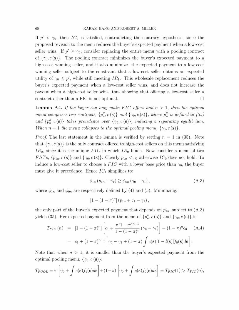
60 KARAM KANG AND ROBERT A. MILLER
If p′ < γ0, then IC0 is satisfied, contradicting the contrary hypothesis, since the
proposed revision to the menu reduces the buyer’s expected payment when a low-cost
seller wins. If p′ ≥ γ0, consider replacing the entire menu with a pooling contract
of γ0, c (s). The pooling contract minimizes the buyer’s expected payment to a
high-cost winning seller, and it also minimizes the expected payment to a low-cost
winning seller subject to the constraint that a low-cost seller obtains an expected
utility of γ0 ≤ p′, while still meeting IR1. This wholesale replacement reduces the
buyer’s expected payment when a low-cost seller wins, and does not increase the
payout when a high-cost seller wins, thus showing that offering a low-cost seller a
contract other than a FIC is not optimal.
Lemma A4. If the buyer can only make FIC offers and n > 1, then the optimal
menu comprises two contracts, p′′n, c (s) and γ0, c (s), where p′′n is defined in (35)
and p′′n, c (s) takes precedence over γ0, c (s), inducing a separating equilibrium.
When n = 1 the menu collapses to the optimal pooling menu, γ0, c (s).
Proof. The last statement in the lemma is verified by setting n = 1 in (35). Note
that γ0, c (s) is the only contract offered to high-cost sellers on this menu satisfying
IR0, since it is the unique FIC in which IR0 binds. Now consider a menu of two
FIC’s, p1n, c (s) and γ0, c (s). Clearly p1n < c0 otherwise IC0 does not hold. To
induce a low-cost seller to choose a FIC with a lower base price than γ0, the buyer
must give it precedence. Hence IC1 simplifies to:
φ1n (p1n − γ1) ≥ φ0n (γ0 − γ1) , (A.3)
where φ1n and φ0n are respectively defined by (4) and (5). Minimizing:
[1− (1− π)n] (p1n + c1 − γ1) ,
the only part of the buyer’s expected payment that depends on p1n, subject to (A.3)
yields (35). Her expected payment from the menu of p′′n, c (s) and γ0, c (s) is:
TFIC (n) = [1− (1− π)n]
[c1 +
π(1− π)n−1
1− (1− π)n(γ0 − γ1)
]+ (1− π)nc0 (A.4)
= c1 + (1− π)n−1
[γ0 − γ1 + (1− π)
∫c(s)[1− l(s)]f0(s)ds
].
Note that when n > 1, it is smaller than the buyer’s expected payment from the
optimal pooling menu, γ0, c (s):
TPOOL = π
[γ0 +
∫c(s)f1(s)ds
]+(1−π)
[γ0 +
∫c(s)f0(s)ds
]= TFIC(1) > TFIC(n),
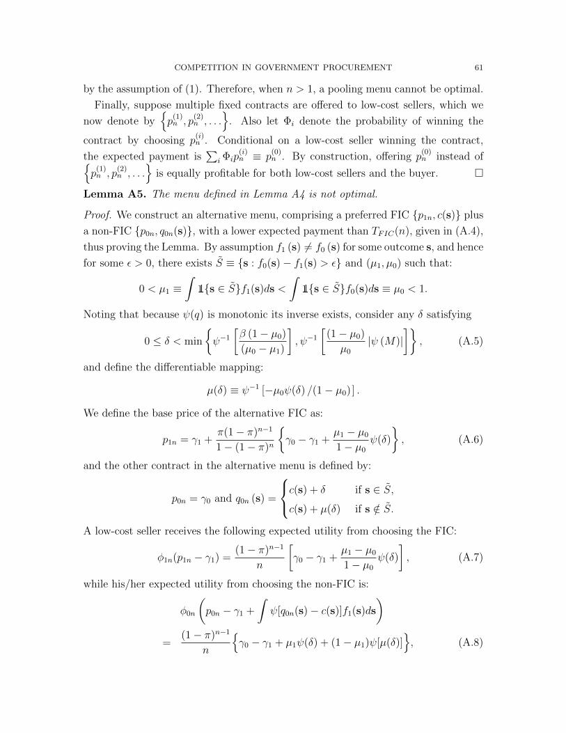
COMPETITION IN GOVERNMENT PROCUREMENT 61
by the assumption of (1). Therefore, when n > 1, a pooling menu cannot be optimal.
Finally, suppose multiple fixed contracts are offered to low-cost sellers, which we
now denote byp
(1)n , p
(2)n , . . .
. Also let Φi denote the probability of winning the
contract by choosing p(i)n . Conditional on a low-cost seller winning the contract,
the expected payment is∑
i Φip(i)n ≡ p
(0)n . By construction, offering p
(0)n instead of
p(1)n , p
(2)n , . . .
is equally profitable for both low-cost sellers and the buyer.
Lemma A5. The menu defined in Lemma A4 is not optimal.
Proof. We construct an alternative menu, comprising a preferred FIC p1n, c(s) plus
a non-FIC p0n, q0n(s), with a lower expected payment than TFIC(n), given in (A.4),
thus proving the Lemma. By assumption f1 (s) 6= f0 (s) for some outcome s, and hence
for some ε > 0, there exists S ≡ s : f0(s)− f1(s) > ε and (µ1, µ0) such that:
0 < µ1 ≡∫1s ∈ Sf1(s)ds <
∫1s ∈ Sf0(s)ds ≡ µ0 < 1.
Noting that because ψ(q) is monotonic its inverse exists, consider any δ satisfying
0 ≤ δ < min
ψ−1
[β (1− µ0)
(µ0 − µ1)
], ψ−1
[(1− µ0)
µ0
|ψ (M)|]
, (A.5)
and define the differentiable mapping:
µ(δ) ≡ ψ−1 [−µ0ψ(δ) /(1− µ0) ] .
We define the base price of the alternative FIC as:
p1n = γ1 +π(1− π)n−1
1− (1− π)n
γ0 − γ1 +
µ1 − µ0
1− µ0
ψ(δ)
, (A.6)
and the other contract in the alternative menu is defined by:
p0n = γ0 and q0n (s) =
c(s) + δ if s ∈ S,
c(s) + µ(δ) if s /∈ S.
A low-cost seller receives the following expected utility from choosing the FIC:
φ1n(p1n − γ1) =(1− π)n−1
n
[γ0 − γ1 +
µ1 − µ0
1− µ0
ψ(δ)
], (A.7)
while his/her expected utility from choosing the non-FIC is:
φ0n
(p0n − γ1 +
∫ψ[q0n(s)− c(s)]f1(s)ds
)=
(1− π)n−1
n
γ0 − γ1 + µ1ψ(δ) + (1− µ1)ψ[µ(δ)]
, (A.8)
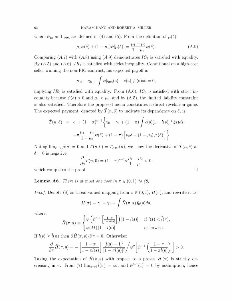
62 KARAM KANG AND ROBERT A. MILLER
where φ1n and φ0n are defined in (4) and (5). From the definition of µ(δ):
µ1ψ(δ) + (1− µ1)ψ[µ(δ)] =µ1 − µ0
1− µ0
ψ(δ). (A.9)
Comparing (A.7) with (A.8) using (A.9) demonstrates IC1 is satisfied with equality.
By (A.5) and (A.6), IR1 is satisfied with strict inequality. Conditional on a high-cost
seller winning the non-FIC contract, his expected payoff is
p0n − γ0 +
∫ψ[q0n(s)− c(s)]f0(s)ds = 0,
implying IR0 is satisfied with equality. From (A.6), IC0 is satisfied with strict in-
equality because ψ(δ) > 0 and µ1 < µ0, and by (A.5), the limited liability constraint
is also satisfied. Therefore the proposed menu constitutes a direct revelation game.
The expected payment, denoted by T (n, δ) to indicate its dependence on δ, is:
T (n, δ) = c1 + (1− π)n−1
γ0 − γ1 + (1− π)
∫c(s)[1− l(s)]f0(s)ds
+πµ1 − µ0
1− µ0
ψ(δ) + (1− π)[µ0δ + (1− µ0)µ (δ)
].
Noting limδ→0 µ(δ) = 0 and T (n, 0) = TFIC(n), we show the derivative of T (n, δ) at
δ = 0 is negative:∂
∂δT (n, 0) = (1− π)n−1π
µ1 − µ0
1− µ0
< 0,
which completes the proof.
Lemma A6. There is at most one root in π ∈ (0, 1) to (8).
Proof. Denote (8) as a real-valued mapping from π ∈ (0, 1), H(π), and rewrite it as:
H(π) = γ0 − γ1 −∫H(π, s)f0(s)ds,
where:
H(π, s) ≡
ψ(ψ′−1
[1−π
1−πl(s)
])[1− l(s)] if l(s) < l(π),
ψ(M) [1− l(s)] otherwise.
If l(s) ≥ l(π) then ∂H(π, s)/∂π = 0. Otherwise:
∂
∂πH(π, s) = −
[1− π
1− πl(s)
][l(s)− 1]2
[1− πl(s)]2
/ψ′′[ψ′−1
(1− π
1− πl(s)
)]> 0.
Taking the expectation of H(π, s) with respect to s proves H (π) is strictly de-
creasing in π. From (7) limπ→0 l(π) = ∞, and ψ′−1(1) = 0 by assumption; hence
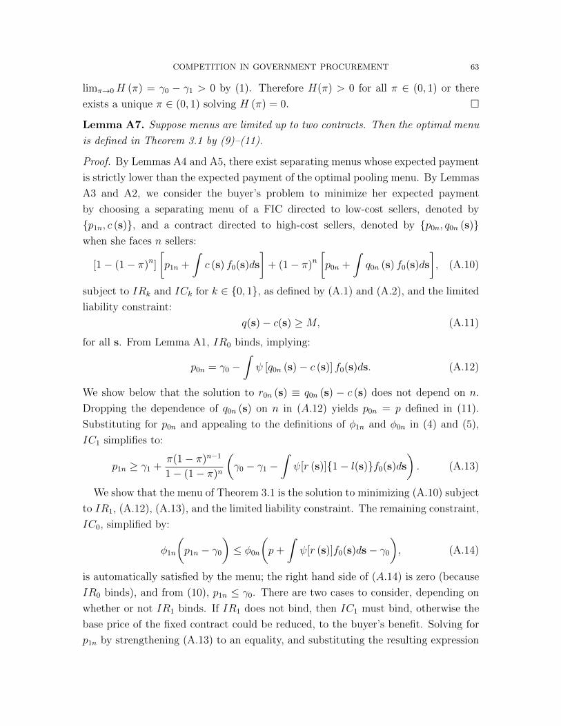
COMPETITION IN GOVERNMENT PROCUREMENT 63
limπ→0H (π) = γ0 − γ1 > 0 by (1). Therefore H(π) > 0 for all π ∈ (0, 1) or there
exists a unique π ∈ (0, 1) solving H (π) = 0.
Lemma A7. Suppose menus are limited up to two contracts. Then the optimal menu
is defined in Theorem 3.1 by (9)–(11).
Proof. By Lemmas A4 and A5, there exist separating menus whose expected payment
is strictly lower than the expected payment of the optimal pooling menu. By Lemmas
A3 and A2, we consider the buyer’s problem to minimize her expected payment
by choosing a separating menu of a FIC directed to low-cost sellers, denoted by
p1n, c (s), and a contract directed to high-cost sellers, denoted by p0n, q0n (s)when she faces n sellers:
[1− (1− π)n]
[p1n +
∫c (s) f0(s)ds
]+ (1− π)n
[p0n +
∫q0n (s) f0(s)ds
], (A.10)
subject to IRk and ICk for k ∈ 0, 1, as defined by (A.1) and (A.2), and the limited
liability constraint:
q(s)− c(s) ≥M, (A.11)
for all s. From Lemma A1, IR0 binds, implying:
p0n = γ0 −∫ψ [q0n (s)− c (s)] f0(s)ds. (A.12)
We show below that the solution to r0n (s) ≡ q0n (s) − c (s) does not depend on n.
Dropping the dependence of q0n (s) on n in (A.12) yields p0n = p defined in (11).
Substituting for p0n and appealing to the definitions of φ1n and φ0n in (4) and (5),
IC1 simplifies to:
p1n ≥ γ1 +π(1− π)n−1
1− (1− π)n
(γ0 − γ1 −
∫ψ[r (s)]1− l(s)f0(s)ds
). (A.13)
We show that the menu of Theorem 3.1 is the solution to minimizing (A.10) subject
to IR1, (A.12), (A.13), and the limited liability constraint. The remaining constraint,
IC0, simplified by:
φ1n
(p1n − γ0
)≤ φ0n
(p+
∫ψ[r (s)]f0(s)ds− γ0
), (A.14)
is automatically satisfied by the menu; the right hand side of (A.14) is zero (because
IR0 binds), and from (10), p1n ≤ γ0. There are two cases to consider, depending on
whether or not IR1 binds. If IR1 does not bind, then IC1 must bind, otherwise the
base price of the fixed contract could be reduced, to the buyer’s benefit. Solving for
p1n by strengthening (A.13) to an equality, and substituting the resulting expression
64 KARAM KANG AND ROBERT A. MILLER
for p1n and p0n using (A.12) into (A.10), we obtain the buyer’s expected payment to
a winning seller as:
[1− (1− π)n]
[γ1 +
π(1− π)n−1
1− (1− π)n
(γ0 − γ1 −
∫ψ[r (s)]1− l(s)f0(s)ds
)+
∫c (s) f1(s)ds
]+ (1− π)n
[γo −
∫ψ [r (s)] f0(s)ds +
∫q (s) f0(s)ds
].
Simplifying the equation, we have:
c1 + (1− π)n−1
[(1− π)(c0 − c1) + π(γ0 − γ1) + Γ
], (A.15)
where Γ is defined by (15), which we reproduce here:
Γ ≡ (1− π)
∫ r(s)− ψ[r(s)]
f0(s)ds− π
∫ψ[r(s)] [1− l(s)] f0(s)ds.
The (scaled) Lagrangian for the cost minimization problem can now be expressed as:∫ [(1− π)
r(s)− ψ[r(s)]
− πψ[r(s)][1− l(s)]− κ1 (s) [r(s)−M ]
]f0(s)ds,
where κ1 (s) ≥ 0 denotes the Kuhn Tucker multiplier for the limited liability con-
straint, (A.11). The first order condition with respect to q(s) is:
(1− π) (1− ψ′[r(s)])− πψ′[r(s)][1− l(s)]− κ1 (s) = 0.
Rearranging terms we obtain:
ψ′ [r(s)] =1− π − κ1 (s)
1− πl(s). (A.16)
If l(s) < l(π), then r(s) = ψ′−1 [(1− π) /[1− πl(s)] ] > M and hence κ1 (s) = 0. If
l(s) ≥ l(π), then κ1 (s) > 0 and r(s) = M .
If IR1 binds then p1n = γ1. Substituting for p1n and p using (A.12), we obtain the
buyer’s expected payment, (A.10), as:
[1− (1− π)n]
[γ1 +
∫c (s) f1(s)ds
]+ (1− π)n
[γ0 +
∫ −ψ [r (s)] + q (s)
f0(s)ds
],
which can be further simplified as:
c1 + (1− π)n[(1− π)(c0 − c1) + π(γ0 − γ1) +
∫ r(s)− ψ[r(s)]
f0(s)ds
].

COMPETITION IN GOVERNMENT PROCUREMENT 65
Substituting for p1n in (A.13) yields:
γ0 − γ1 ≤∫ψ[r (s)]1− l(s)f0(s)ds. (A.17)
Let κ1 (s) ≥ 0 denote the Kuhn Tucker multiplier for the limited liability constraint,
(A.11). If IC1 does not bind, then the first order condition with respect to r(s) for
the Kuhn Tucker formulation is:
1− ψ′[r (s)] = κ1 (s) .
If r (s) > M , then the complementary slackness condition requires κ1 (s) = 0, and
hence 1 = ψ′[r (s)] implying r (s) = 0. Therefore, either r (s) = M or r (s) = 0.
Let us define SM as the set of contract outcomes such that r(s) = M . The buyer’s
expected payment can now be written as:
c1+(1−π)n
(1−π)(c0−c1)+π(γ0−γ1)+[M−ψ(M)]
∫1s ∈ SMf0(s)ds
. (A.18)
By inspection (A.18) is increasing in∫1s ∈ SMf0(s)ds, while setting
∫1s ∈
SMf0(s)ds = 0 does not satisfy IC1, (A.17). This implies that when IR1 binds, IC1
does too; in other words (A.17) holds with equality. Now the (scaled) Lagrangian for
the minimization problem can be written as:∫ (r (s)− ψ[r (s)]
)− κ1 (s) [r (s)−M ]
f0(s)ds (A.19)
+κ2
γ0 − γ1 −
∫ψ[r (s)][1− l(s)]f0(s)ds
,
where κ2 denotes the Kuhn Tucker multiplier for (A.17). The first order condition
with respect to r (s) is:
1− ψ′[r (s)]− κ1 (s)− κ2ψ′[r (s)][1− l(s)] = 0,
which can be expressed:
ψ′[r (s)] =1− κ1 (s)
1 + κ2[1− l(s)]. (A.20)
Since (A.19) does not depend on π, neither does q(s) nor κ1 (s) and κ2. Noting that
π solves both first order conditions (A.16) and (A.20), we equate the two and deduce
κ2 = π /(1− π) . Substituting for κ2 in (A.20), the solution for r (s) follows by setting
π = π in (9). It immediately follows from (10) that if H(π) > 0 then pn > γ1, but
if H(π) ≤ 0 then pn = γ1. Appealing to Lemma A6, we conclude if π < π, then
H(π) > 0 and IR1 not bind; otherwise π ≥ π, then H(π) ≤ 0 and IR1 binds.
66 KARAM KANG AND ROBERT A. MILLER
C.2. Proof of Theorem 3.1. By Lemma A2 it is not optimal to offer a separating
menu in which contracts directed to high-cost sellers are prioritized, that is ranked
above low-cost sellers. By Lemma A3 it is optimal to offer low-cost sellers a FIC.
Given Lemmas A4 and A7, the expected payment from offering a menu of FIC’s to
both seller types (including the optimal pooling menu when facing a single bidder),
TFIC (n), exceeds T (n). Then Lemma A7 establishes the optimal menu when the
buyer is constrained to offer two-contract menus only.
We now show additional contracts are redundant. Noting that low-cost sellers are
offered a FIC, exactly the same arguments used in the proof of Lemma A4 apply
here. Therefore offering multiple full insurance contracts to low-cost sellers does not
reduce the expected payment. Also every contract offered to high-cost sellers must
individually satisfy IC1 and IR0, the latter with equality by Lemma A1. If any
two contracts on the menu do not generate the same expected payment to a high-
cost seller, then offering the more expensive one is suboptimal. This proves the first
statement of the theorem.
C.3. Proof of Corollary 3.1. To prove (14) note that the optimal strategy for a
buyer with full information is to approach a low-cost seller if there is one, and offer
the initial cost as a base price by setting pkn = γk plus full insurance qkn (s) = c (s)
for k ∈ 0, 1, efficiently extracting all the project surplus. Thus:
TU(n) = [1− (1− π)n] c1 + (1− π)n c0 = c1 + (1− π)n (c0 − c1) ,
as required. From (A.4) and (14):
TFIC(n)− TU(n)
= c1 + (1− π)n[c0 − c1 +
π
1− π(γ0 − γ1)
]− c1 − (1− π)n (c0 − c1)
= π(1− π)n−1 (γ0 − γ1) ,
which proves (13). Finally appealing to (10) and (11) we can express T (n) as (A.15).
Thus, T (n) = TFIC(n) + (1− π)n−1 Γ. By inspection Γ < 0 implying T (n) < TFIC(n)
and TU(n) ≤ T (n) since the cost minimization problem underpinning TU(n) imposes
fewer constraints than the problem associated with T (n).
C.4. Proof of Corollary 3.2. In the extended model where sellers choose whether
to pay the entry cost, κs, the individual rationality constraint as in (A.1) becomes:
maxj∈J
ωjk −
κsφjn
≡ ω∗k ≥ 0, (A.21)
COMPETITION IN GOVERNMENT PROCUREMENT 67
given a menu pjn, qjn(s)Jj=0 ≡ J and n sellers. Recall that ωjk is the expected
utility to a type k from winning the procurement by choosing pjn, qjn(s) from the
menu; φjn is the probability of winning the procurement when there are n sellers
participating in the procurement process and a given seller chooses contract j. In
contrast, the incentive compatibility applies after the entry costs have been paid, and
hence remain unchanged from (A.2).
Lemmas A1–A6 can be adapted to this extended case with minimal notational
changes. There is essentially no change to the proof of these lemmas, aside from
replacing γk with γ∗kn ≡ γk +κ/φkn. Therefore the buyer’s problem has the same rep-
resentation as when sellers incur no entry costs, (A.10): given n sellers she minimizes
her expected payment from choosing a separating menu of a full-insurance contract
directed to low-cost sellers, now denoted by p∗1n, c (s), and a contract directed to
high-cost sellers, denoted by p∗0n, q∗0n(s), subject to IR∗k and ICk for k ∈ 0, 1, as
defined by (A.21) and (A.2), plus the limited liability constraint (A.11).
Following the basic model, the solution q∗0n(s) does not depend on n, so we write
r∗(s) ≡ q∗0n(s)− c(s), dropping the subscript n. Since IR0 binds (Lemma A1):
p∗0n = γ∗0n −∫ψ [r∗ (s)] f0(s)ds. (A.22)
Substituting for p∗0n, IC1 an be expressed as:
φ1n
(p∗1n − γ1 −
κsφ1n
)≥ φ0n
(γ∗0n −
∫ψ[r∗ (s)]1− l(s)f0(s)ds− γ1 −
κsφ0n
),
where φkn is defined in (4) and (5) for k ∈ 0, 1. Appealing to the definitions of γ∗knand φkn and simplifying:
p∗1n ≥ γ∗1n +π(1− π)n−1
1− (1− π)n
(γ0 − γ1 −
∫ψ[r∗ (s)]1− l(s)f0(s)ds
). (A.23)
The proof of the corollary is completed by obtaining the solution to minimizing (A.10)
subject to IR∗1, (A.22), (A.23), and the limited liability constraint. As before, the
remaining constraint, IC∗0 , is automatically satisfied by the menu. The optimization
problem determining r∗(s) is identical to its analogue solving for r(s), and hence they
share the same solution. The remainder of the proof then runs parallel to the case
where there are no entry costs borne by sellers.
C.5. Proof of Corollary 3.3. Given n sellers, the expected benefits from using the
menu of Theorem 3.1 are:
B (n) ≡ b1 − (1− π)n (b1 − b0) .

68 KARAM KANG AND ROBERT A. MILLER
The expected benefits from a menu with a separating equilibrium that prioritizes
contracts a high-cost seller selects are:
B1 (n) ≡ b0 + πn (b1 − b0) .
The expected benefits from randomly selecting a seller are:
B2 (n) ≡ b1 − (1− π) (b1 − b0) .
Since b1 ≥ b0:
B (n)−B1 (n) = [1− πn − (1− π)n] (b1 − b0) ≥ 0,
B (n)−B2 (n) = (1− π)[1− (1− π)n−1
](b1 − b0) ≥ 0.
Let T1 (n) denote the minimal expected cost of implementing a menu with a sepa-
rating equilibrium that prioritizes contracts a high-cost seller selects, if such a menu
exists; otherwise set T1 (n) = ∞. Let T2 (n) denote the minimal cost of a menu
that randomly selects a seller (a single item full insurance contract with base price
γ1). Then by definition T (n) ≤ min T1 (n) , T2 (n). Therefore B (n) − T (n) ≥max B1 (n)− T1 (n) , B2 (n)− T2 (n).
Appendix D. Proving Identification
D.1. Proof of Lemma 4.1(i). By A3 v (l, π) satisfies (18). Totally differentiating
(18) with respect to π and making ∂v (l, π) /∂π the subject of the resulting equation:
∂v (l, π)
∂π=
l − 1
ψ′′ (r) (1− πl)2 . (A.24)
By assumption ψ′′ (r) < 0, implying ∂v (l, π) /∂π R 0 when l R 1. From (18) it follows
that v (l, π) R 0 when l R 1. Combining both sets of inequalities ∂v (l, π) /∂π R 0
when v (l, π) R 0, as claimed.
D.2. Proof of Lemma 4.1 (ii). Rewriting (10) to make the dependence of pn on π
explicit:
pn(π) = γ1 (π) +π(1− π)n−1
1− (1− π)n
[γ0 (π)− γ1 (π)−
∫ψ (v [l (s) , π]) [1− l (s)] f0(s)ds
]≡ γ1 (π) + Ψ0,n (π) [γ0 (π)− γ1 (π)−Ψ1 (π)] ,
and hence:
p′n(π) = γ′1 (π)+Ψ′0,n (π) [γ0 (π)− γ1 (π)−Ψ1 (π)]+Ψ0,n (π) [γ′0 (π)− γ′1 (π)−Ψ′1 (π)] .
COMPETITION IN GOVERNMENT PROCUREMENT 69
By definition Ψ0,n (π) > 0, γ′1 (π) by A4, and γ′0 (π) − γ′1 (π) ≤ 0 by A5. By A3
IR1 does not bind, implying γ0 (π)− γ1 (π)− Ψ1 (π) > 0. Completing the proof, we
now show that Ψ′0,n (π) ≤ 0 implying the second expression is nonpositive, and that
Ψ′1 (π) > 0, implying the third expression is negative. With regards Ψ′0,n (π):
∂
∂πln [Ψ0,n (π)] =
1− nπ − (1− π)n
π (1− π) [1− (1− π)n].
The derivative is zero at n = 1 and −π2 at n = 2. Now suppose it is negative for all
n ∈ 2, . . . , n. For n+ 1 the denominator is positive and the numerator is:
1− (n+ 1) π − (1− π) (1− π)n < π (1− π)n − π < 0.
The first inequality follows from an induction hypothesis, and the second one from
the inequalities 0 < π < 1. Therefore Ψ′0,n (π) ≤ 0 for all (π, n). To sign Ψ′1 (π):
Ψ′1 (π) =
∫ψ′ (v [l (s) , π])
∂v [l (s) , π]
∂π[1− l (s)] f0(s)ds
=
∫ [1− π
1− πl (s)
]∂v [l (s) , π]
∂π[1− l (s)] f0(s)ds.
Appealing to A3, the second equality uses (18) to substitute out ψ′ [v (s, π)]. Totally
differentiating (18) with respect to π and making ∂v (l, π) /∂π the subject of the
resulting equation:∂v (l, π)
∂π=
l − 1
ψ′′ (r) (1− πl)2 . (A.25)
Using (A.25) to substitute out ∂v (l, π) /∂π ,
Ψ′1 (π) =
∫(π − 1) [1− l (s)]2
ψ′′ (v [l (s) , π]) [1− πl (s)]3f0(s)ds > 0.
The inequality follows from ψ′′ (r) < 0 and the assumption of an interior solution.
D.3. Proof of Lemma 4.1 (iii). Let:
m(l, π) ≡ ψ′ [v (l, π)]∂v (l, π)
∂π.
From (18) the first order condition for an interior solution can be rewritten as:
v (l, π) = ψ′−1
(1− π1− πl
), (A.26)
70 KARAM KANG AND ROBERT A. MILLER
and taking the derivative of v (l, π) with respect to π:
∂v (l, π)
∂π=
(ψ′′[ψ′−1
(1− π1− πl
)])−1l − 1
(1− πl)2.
Therefore:
m (l, π) =
(ψ′′[ψ′−1
(1− π1− πl
)])−1(1− π) (l − 1)
(1− πl)3 . (A.27)
Totally differentiating with respect to π the base price for the high-cost contract
defined in (11), and appealing to (A.27) yields:
p′ (π) = γ′0 (π)−∫m [l(s), π] f0(s)ds (A.28)
= γ′0 (π)−∫ (
ψ′′[ψ′−1
(1− π
1− πl(s)
)])−1(1− π) [l(s)− 1]
[1− πl(s)]3f0(s)ds
≡ γ′0 (π)−Ψ0 (π) .
It now follows that p (π) is increasing in π if Ψ0 (π) ≤ γ′0 (π) for all π, and decreasing
in π if Ψ0 (π) ≥ γ′0 (π) for all π.
D.4. Proof of Lemma 4.2. The joint probability that the contract type is fixed
and π ≤ π can be expressed as:
Pr π ≤ π, k = 1 |y, n = Fπ|y,n,k (π |y, n, 1) Pr (k = 1 |y, n)
=
∫ π
π=π
fπ|y,n (π |y, n) [1− (1− π)n] dπ.
Taking the derivative with respect to π yields:
fπ|y,n ,k (π |y, n, 1) Pr (k = 1 |y, n) = fπ|y,n (π |y, n) [1− (1− π)n] . (A.29)
Similarly:
Pr π ≤ π, k = 0 |y, n = Fπ|y,n,k (π |y, n, 0) Pr (k = 0 |y, n)
=
∫ π
π=π
fπ|y,n (π |y, n) (1− π)n dπ,
and taking the derivative with respect to π yields:
fπ|y,n,k (π |y, n, 0) Pr (k = 1 |y, n) = fπ|y,n (π |y, n) (1− π)n . (A.30)
Rearranging the quotient of (A.29) and (A.30) to make fπ|y,n,1 (π |y, n, 1) the subject
of the resulting equation, and relabeling π as π, we obtain (20). Integrating (20) over
COMPETITION IN GOVERNMENT PROCUREMENT 71
π:
1 =Pr(k = 0|y, n)
Pr(k = 1|y, n)
∫[1− (1− π)n]
(1− π)nfπ|y,n,k(π|y, n, 0)dπ. (A.31)
Rearranging terms to make Pr(k = 0|y, n) the subject of the equation:
Pr(k = 0|y, n) =
(∫(1− π)−nfπ|v,n,k(π|y, n, 0)dπ
)−1
. (A.32)
The identification of fπ|y,n (π|y, n) and (21) now follow by expressing fπ|y,n,k(π|y, n, 1)
and Pr(k = 0|y, n) as functions of fπ|y,n,k(π|y, n, 0) using (20) and (A.32), and then
appealing to the identity:
fπ|y,n(π|y, n) = fπ|y,n,0(π|y, n, 0) Pr(k = 0|y, n) + fπ|y,n,k(π|y, n, 1) Pr(k = 1|y, n).
Noting that Pr(y, n) is identified from the data and that both contracts in the sep-
arating menu occur with positive probabilities for any π in the support, fπ(π) =
fπ|y,n(π|y, n) Pr(y, n) is also identified.
D.5. Proof of Lemma 4.3. To prove the first equation in (23) set n = 1 in (10) to
obtain:
p1 (π) = γ0 (π)−∫ψ[r (s)] [1− l (s)] f0(s)ds.
Subtract γ1 (π) from both sides and substitute the right hand side of the resulting
expression back into (10) to obtain:
pn (π) = γ1 (π) +π (1− π)n−1
1− (1− π)n[p1 (π)− γ1 (π)] .
The first equation in (23) follows. To prove the second equation in (23), we rearrange
(18) using (A.26), substitute the expression into (11), and make γ0 (π) the subject of
the equation.
D.6. Proof of Lemma 4.4. Lemma 4.2 identifies fπ|y,n (π|y, n). Therefore, λo(π) is
identified from:
λo(π) =∞∑n=1
(n− 1) Pr(n|π, y = 1) =
∑∞n=1(n− 1)fπ|y,n (π|1, n) Pr(n|y = 1)∑∞
n=1 fπ|y,n (π|1, n) Pr(n|y = 1).
Given this, κ(π) is identified for all values of π satisfying λo(π) > 0 from (24) because
Γ(π), c0(π)−c1(π), and γ0(π)−γ1(π) are identified from previous steps. If λo(π) = 0,
κ(π) ≥ π π[γ0 (π)− γ1 (π)] + (1− π)[c0 (π)− c1 (π)] + Γ(π) .
thus establishing the identified lower bound.
72 KARAM KANG AND ROBERT A. MILLER
D.7. Proof of Lemma 4.5. Appealing to (17), the buyer solicits competitive bids if
and only if η ≤ Ω(π), implying Fη[Ω(π)] = Pr (y = 1|π). We have previously identified
all components of Ω(π), and hence Ω(π). Since Pr(y = 1|π) = fπ|y (π |y ) Pr (y) /fπ (π) ,
and (y, n) are observed variables (implying their joint distribution is identified),
Pr(y = 1|π) is identified from (21). Therefore Fη (η) is identified on Υ.
Appendix E. Estimation Procedure
This appendix elaborates on our sequential estimation procedure described in Sec-
tion 5.2, and includes the proof of Lemma 5.1. As in the text, we assume the data is
generated by θ∗ and denote our estimates by θ. For conciseness we abbreviate (x, z)
with x.
E.1. Contract Outcomes and Distribution of π. For each h ∈ 1, 2, 3 the LIML
estimator of θ∗s2h , defined in (29) and (30), is:
θs2h = arg maxθs2h
∑i
ki log [f1,s2h(s2h|x1; θs2h)] + (1− ki) log [f0,s2h(s2h|x1; θs2h)] .
Noting that f1,s1h|s2h (s1h|s2h,x1; θs1h) does not depend on θs1h,0 (to be estimated in
the next step), the LIML estimator for all the elements θ∗s1h except θ∗s1h,0 defined in
(27) and (28), is:
θ′s1h = arg maxθ′s1h
∑i
ki log[f1,s1h|s2h
(s1h|s2h,x1; θ′s1h
)].
Following the procedure of 5.2.2, we estimate θ∗π and fπ(π|x; θ∗π).
E.2. Seller Costs and Risk Preferences. For notational convenience, let θϕ ≡(θϕ1 , θϕ2) where θϕ1 ≡
(θ′s1 , θs2
), estimated in a previous step, and θϕ2 ≡ θc, θψ, θs1,0 ,M,
the parameters remaining that characterize sellers costs. Following Lemma A6, let
π(x, π; θϕ) uniquely solve:
γ0(x1, π; θc)− γ1(x1, π; θc) =
∫ [f1(s|x1, θs)− f0(s|x1, θs)
]×
ψ
(max
−ex1θψ ln
(1− π
1− πl(s|x1; θs)
),M
∣∣∣∣x1; θψ
)ds.
COMPETITION IN GOVERNMENT PROCUREMENT 73
Theorem 3.1 implies prices for the optimal menu in the parameterization are:
p1n(x1, π; θϕ) = γ1(x1, π; θc) +π(1− π)n−1
1− (1− π)n
[γ0(x1, π; θc)− γ1(x1, π; θc)] (A.33)
−∫ψ [q0(s,x1, π; θϕ)− c(s)|x1; θψ] [f0(s|x1; θs)− f1(s|x1; θs)] ds
,
q0(s,x1, π; θϕ) = c(s) + max
−ex1θψ ln
(1−minπ, π(x1, π; θϕ)
1−minπ, π(x1, π; θϕ)l(s|x1; θs)
),M
.
We obtain θϕ2 as follows:
θϕ2 = arg minθϕ2
∑i
ki
[pi −
∫p1n(x1i, π; θϕ1 , θϕ2)fπ|y,n,k(π|yi, ni, 1, xi; θπ,yi,ni)dπ
]2
+(1− ki)[pi −
∫p0(x1i, π; θϕ1 , θϕ2)fπ|y,n,k(π|yi, ni, 0, xi; θπ,yi,ni)dπ
]2
+(1− ki)[qi −
∫q0(si,x1i, π; θϕ1 , θϕ2)fπ|y,n,k(π|yi, ni, 0, xi; θπ,yi,ni)dπ.
]2.
We compute integrals over π and s numerically: for the integration over π, we use
Legendre-Gauss quadrature with 50 points from [0.01, 0.99]; for the integration over
s, we employ Monte Carlo simulations using 5,000 points of a six-dimensional Halton
sequence.
E.3. Buyer Search Costs and Solicitation Costs. We obtain λo(x, π; θπ), using
the parameters estimated from a previous step and Lemma 5.1, and the proof of the
lemma is below:
Proof. Note that:
λo(x, π) = E[(n− 1)|y = 1, x, π] =∞∑n=1
(n− 1) Pr(n|y = 1, x, π)
=
∑∞n=1(n− 1) Pr(n, π|y = 1, x)
fπ|y(π|y = 1, x)
=
∑∞n=1(n− 1)fπ|y,n(π|y = 1, n, x) Pr(n|y = 1, x)∑∞
n=1 fπ|y,n(π|y = 1, n, x) Pr(n|y = 1, x)
=
∑∞n=1(n− 1)
∑1k=0 fπ|y,n,k(π|y = 1, n, k) Pr(n, k|y = 1, x)∑∞
n=1
∑1k=0 fπ|y,n,k(π|y = 1, n, k) Pr(n, k|y = 1, x)
.
74 KARAM KANG AND ROBERT A. MILLER
A consistent estimator of Pr(n, k|y = 1, x) is:
Pr(n, k|y = 1, x) =
∑Ii=1 1(ni, ki, yi, xi) = (n, k, 1, x)∑I
i=1 1(yi, xi) = (1, x). (A.34)
If fπ|y,n,k (π|1, ni, ki, xi) was known, a consistent estimator of λo(x, π) is:
λo(x, π) =
∑∞n=1
∑1k=0(n− 1)fπ|y,n,k(π|1, n, k, x)Pr(n, k|y = 1, x)∑∞
n=1
∑1k=0 fπ|y,n,k(π|1, n, k, x)Pr(n, k|y = 1, x)
.
By substituting (A.34) for Pr(n, k|y = 1, x):
λo(x, π) =
∑∞n=1
∑1k=0(n− 1)fπ|y,n,k(π|1, n, k, x)
∑Ii=1 1(ni, ki, yi, xi) = (n, k, 1, x)∑∞
n=1
∑1k=0 fπ|y,n,k(π|1, n, k, x)
∑Ii=1 1(ni, ki, yi, xi) = (n, k, 1, x)
=
∑Ii=1(ni − 1)fπ|y,n,k(π|1, ni, ki, x)1(yi, xi) = (1, x)∑I
i=1 fπ|y,n,k(π|1, ni, ki, x)1(yi, xi) = (1, x). (A.35)
Substituting fπ|y,n,k(π|1, ni, ki, xi; θπ) for fπ|y,n,k(π|1, ni, ki, xi) proves the lemma.
Then, we obtain κ(x, π, θϕ) from (32). With reference to (33), the estimator for θ∗ηis:
θη = arg maxθη
∑i
yi log Pr(y = 1|xi; θη, θϕ, θπ) + (1− yi) log Pr(y = 0|xi; θη, θϕ, θπ),
where:
Pr(y = 1|x; θη, θϕ, θπ) =
∫Φ
(Ω(x, π; θϕ, θπ)− [xθηx + πθη1 + π2θη2 ]
θηv
)fπ(π|x, θπ)dπ,
and:
Ω(x, π; θϕ, θπ) =
1− exp[λo(x, π; θπ)
] [πγ0(x1, π; θc)− γ1(x1, π; θc)
+(1− π)
c0(x1, π; θc)− c1(x1, π; θc)
+ Γ(x1, π; θϕ)
]− κ(x, π; θϕ, θπ)λo(x, π; θπ).
Appendix F. Implementing Model Fit and Counterfactual Analyses
This section explains on how we calculate the extent of competition for the base
and some of the counterfactual scenarios for Tables 4 and 6, given our model and the
estimated parameters. We continue to abbreviate (x, z) with x.
F.1. Base Scenario. For any given (x, θ), the probability that the buyer chooses
a competitive solicitation, as opposed to working with a default seller, denoted by
COMPETITION IN GOVERNMENT PROCUREMENT 75
Yo(x, π; θ), is:
Yo(x, π; θ) = Φ
(Ω(x, π; θϕ, θπ)− [xθηx + πθη1 + π2θη2]
θηv
).
The optimal search intensity is solved as:
λo (x, π; θϕ, θπ) = max
[0,
1
π
(ln c(x1; θϕ) + Γ(x1, π; θϕ) − lnκ(x, π; θϕ, θπ)
)],
where
c(x1; θϕ) = πγ0(x1; θc)− γ1(x1; θc)+ (1− π)c0(x1; θϕ)− c1(x1; θϕ).
Then the expected number of bids is:
N o(x, π; θ) = 1 + λo (x, π; θϕ, θπ)Yo(x, π; θ).
Table 4 presents the sample average of Yo(x, π; θ) and N o(x, π; θ) evaluated at the
estimated parameter, θ, integrated over π. For example, the predicted value for the
expected number of bids in the table is:
I∑i
∫N o(xi, π; θ
)fπ
(π|xi, θπ
)dπ /I.
F.2. First-price Sealed-bid Auction. If the buyer’s ability to design contracts
is limited so that she can offer full insurance contracts only, then the constrained
optimal search intensity, λFIC (x, π; θ, κ) is:
λFIC (x, π; θϕ, θπ) = max
[0,
1
π
(ln c(x1; θϕ)− lnκ(x, π; θϕ, θπ)
)].
Section 3 has shown that Γ < 0, and therefore, λFIC (x, π; θ, κ) > λ∗ (x, π; θ, κ). The
expected number of bids under this scenario, N FIC(x, π; θ), is:
N FIC(x, π; θ) = 1+λFIC (x, π; θϕ, θπ) Φ
(ΩFIC(x, π; θϕ, θπ)− [xθηx + πθη1 + π2θη2]
θηv
),
where
ΩFIC(x, π; θϕ, θπ) ≡
1− e−λFIC(x,π;θϕ,θπ)πc(x1; θϕ)−κ(x, π; θϕ, θπ)λFIC (x, π; θϕ, θπ) .
Table 6 provides the following:∑i
∫ [N FIC
(xi, π; θ
)−N o
(xi, π; θ
)]fπ
(π|xi, θπ
)dπ /I.
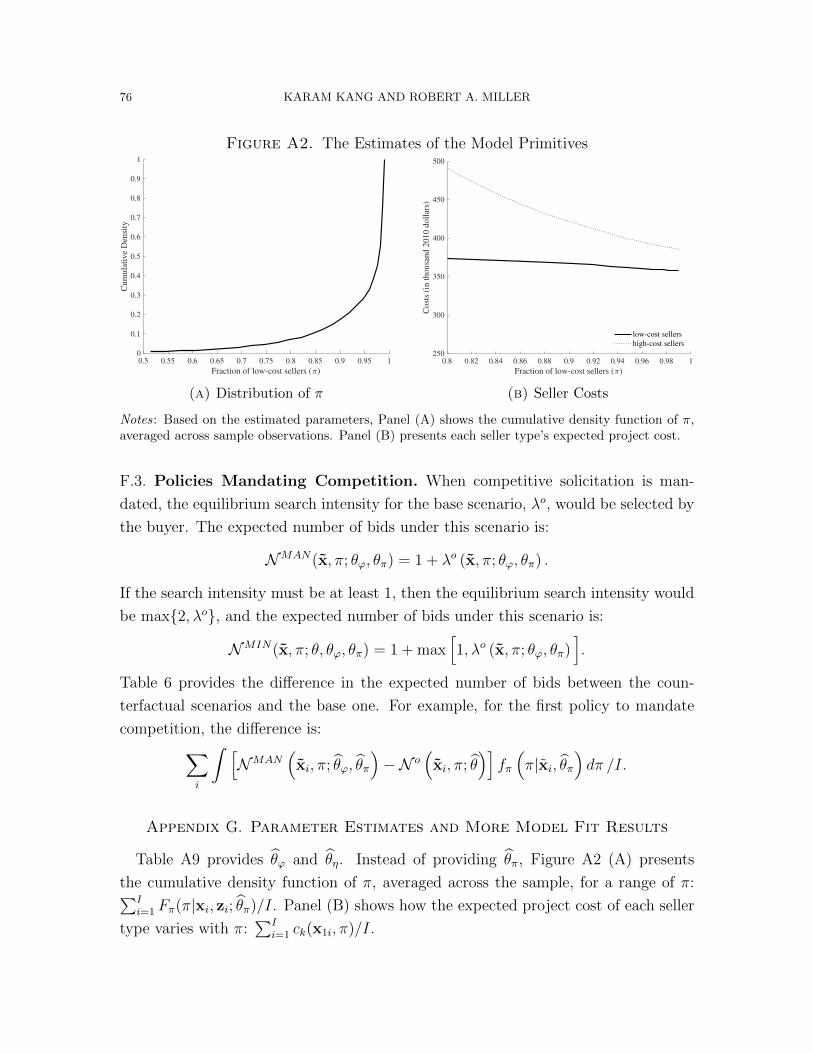
76 KARAM KANG AND ROBERT A. MILLER
Figure A2. The Estimates of the Model Primitives
0.5 0.55 0.6 0.65 0.7 0.75 0.8 0.85 0.9 0.95 1
Fraction of low-cost sellers ( )
0
0.1
0.2
0.3
0.4
0.5
0.6
0.7
0.8
0.9
1
Cu
mu
lati
ve
Den
sity
(a) Distribution of π
0.8 0.82 0.84 0.86 0.88 0.9 0.92 0.94 0.96 0.98 1
Fraction of low-cost sellers ( )
250
300
350
400
450
500
Co
sts
(in
th
ou
san
d 2
01
0 d
oll
ars)
low-cost sellers
high-cost sellers
(b) Seller Costs
Notes: Based on the estimated parameters, Panel (A) shows the cumulative density function of π,averaged across sample observations. Panel (B) presents each seller type’s expected project cost.
F.3. Policies Mandating Competition. When competitive solicitation is man-
dated, the equilibrium search intensity for the base scenario, λo, would be selected by
the buyer. The expected number of bids under this scenario is:
NMAN(x, π; θϕ, θπ) = 1 + λo (x, π; θϕ, θπ) .
If the search intensity must be at least 1, then the equilibrium search intensity would
be max2, λo, and the expected number of bids under this scenario is:
NMIN(x, π; θ, θϕ, θπ) = 1 + max[1, λo (x, π; θϕ, θπ)
].
Table 6 provides the difference in the expected number of bids between the coun-
terfactual scenarios and the base one. For example, for the first policy to mandate
competition, the difference is:∑i
∫ [NMAN
(xi, π; θϕ, θπ
)−N o
(xi, π; θ
)]fπ
(π|xi, θπ
)dπ /I.
Appendix G. Parameter Estimates and More Model Fit Results
Table A9 provides θϕ and θη. Instead of providing θπ, Figure A2 (A) presents
the cumulative density function of π, averaged across the sample, for a range of π:∑Ii=1 Fπ(π|xi, zi; θπ)/I. Panel (B) shows how the expected project cost of each seller
type varies with π:∑I
i=1 ck(x1i, π)/I.
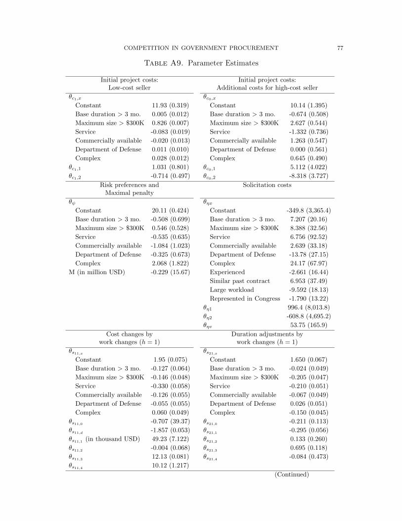
COMPETITION IN GOVERNMENT PROCUREMENT 77
Table A9. Parameter Estimates
Initial project costs: Initial project costs:Low-cost seller Additional costs for high-cost seller
θc1,x θc0,xConstant 11.93 (0.319) Constant 10.14 (1.395)
Base duration > 3 mo. 0.005 (0.012) Base duration > 3 mo. -0.674 (0.508)
Maximum size > $300K 0.826 (0.007) Maximum size > $300K 2.627 (0.544)
Service -0.083 (0.019) Service -1.332 (0.736)
Commercially available -0.020 (0.013) Commercially available 1.263 (0.547)
Department of Defense 0.011 (0.010) Department of Defense 0.000 (0.561)
Complex 0.028 (0.012) Complex 0.645 (0.490)
θc1,1 1.031 (0.801) θc0,1 5.112 (4.022)
θc1,2 -0.714 (0.497) θc0,2 -8.318 (3.727)
Risk preferences and Solicitation costsMaximal penalty
θψ θηxConstant 20.11 (0.424) Constant -349.8 (3,365.4)
Base duration > 3 mo. -0.508 (0.699) Base duration > 3 mo. 7.207 (20.16)
Maximum size > $300K 0.546 (0.528) Maximum size > $300K 8.388 (32.56)
Service -0.535 (0.635) Service 6.756 (92.52)
Commercially available -1.084 (1.023) Commercially available 2.639 (33.18)
Department of Defense -0.325 (0.673) Department of Defense -13.78 (27.15)
Complex 2.068 (1.822) Complex 24.17 (67.97)
M (in million USD) -0.229 (15.67) Experienced -2.661 (16.44)
Similar past contract 6.953 (37.49)
Large workload -9.592 (18.13)
Represented in Congress -1.790 (13.22)
θη1 996.4 (8,013.8)
θη2 -608.8 (4,695.2)
θηv 53.75 (165.9)
Cost changes by Duration adjustments bywork changes (h = 1) work changes (h = 1)
θs11,x θs21,xConstant 1.95 (0.075) Constant 1.650 (0.067)
Base duration > 3 mo. -0.127 (0.064) Base duration > 3 mo. -0.024 (0.049)
Maximum size > $300K -0.146 (0.048) Maximum size > $300K -0.205 (0.047)
Service -0.330 (0.058) Service -0.210 (0.051)
Commercially available -0.126 (0.055) Commercially available -0.067 (0.049)
Department of Defense -0.055 (0.055) Department of Defense 0.026 (0.051)
Complex 0.060 (0.049) Complex -0.150 (0.045)
θs11,0 -0.707 (39.37) θs21,0 -0.211 (0.113)
θs11,d -1.857 (0.053) θs21,1 -0.295 (0.056)
θs11,1 (in thousand USD) 49.23 (7.122) θs21,2 0.133 (0.260)
θs11,2 -0.004 (0.068) θs21,3 0.695 (0.118)
θs11,3 12.13 (0.081) θs21,4 -0.084 (0.473)
θs11,4 10.12 (1.217)
(Continued)
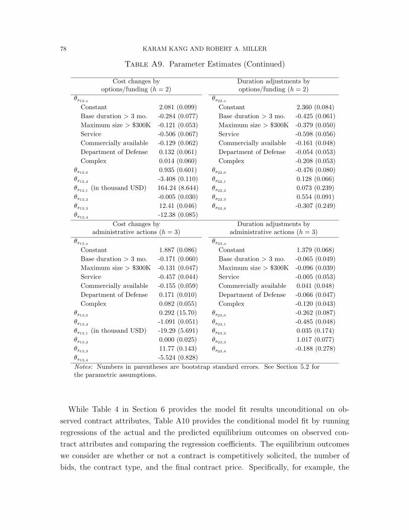
78 KARAM KANG AND ROBERT A. MILLER
Table A9. Parameter Estimates (Continued)
Cost changes by Duration adjustments byoptions/funding (h = 2) options/funding (h = 2)
θs12,x θs22,xConstant 2.081 (0.099) Constant 2.360 (0.084)
Base duration > 3 mo. -0.284 (0.077) Base duration > 3 mo. -0.425 (0.061)
Maximum size > $300K -0.121 (0.053) Maximum size > $300K -0.379 (0.050)
Service -0.506 (0.067) Service -0.598 (0.056)
Commercially available -0.129 (0.062) Commercially available -0.161 (0.048)
Department of Defense 0.132 (0.061) Department of Defense -0.054 (0.053)
Complex 0.014 (0.060) Complex -0.208 (0.053)
θs12,0 0.935 (0.601) θs22,0 -0.476 (0.080)
θs12,d -3.408 (0.110) θs22,1 0.128 (0.066)
θs12,1 (in thousand USD) 164.24 (8.644) θs22,2 0.073 (0.239)
θs12,2 -0.005 (0.030) θs22,3 0.554 (0.091)
θs12,3 12.41 (0.046) θs22,4 -0.307 (0.249)
θs12,4 -12.38 (0.085)
Cost changes by Duration adjustments byadministrative actions (h = 3) administrative actions (h = 3)
θs13,x θs23,xConstant 1.887 (0.086) Constant 1.379 (0.068)
Base duration > 3 mo. -0.171 (0.060) Base duration > 3 mo. -0.065 (0.049)
Maximum size > $300K -0.131 (0.047) Maximum size > $300K -0.096 (0.039)
Service -0.457 (0.044) Service -0.005 (0.053)
Commercially available -0.155 (0.059) Commercially available 0.041 (0.048)
Department of Defense 0.171 (0.010) Department of Defense -0.066 (0.047)
Complex 0.082 (0.055) Complex -0.120 (0.043)
θs13,0 0.292 (15.70) θs23,0 -0.262 (0.087)
θs13,d -1.091 (0.051) θs23,1 -0.485 (0.048)
θs13,1 (in thousand USD) -19.29 (5.691) θs23,2 0.035 (0.174)
θs13,2 0.000 (0.025) θs23,3 1.017 (0.077)
θs13,3 11.77 (0.143) θs23,4 -0.188 (0.278)
θs13,4 -5.524 (0.828)
Notes: Numbers in parentheses are bootstrap standard errors. See Section 5.2 forthe parametric assumptions.
While Table 4 in Section 6 provides the model fit results unconditional on ob-
served contract attributes, Table A10 provides the conditional model fit by running
regressions of the actual and the predicted equilibrium outcomes on observed con-
tract attributes and comparing the regression coefficients. The equilibrium outcomes
we consider are whether or not a contract is competitively solicited, the number of
bids, the contract type, and the final contract price. Specifically, for example, the
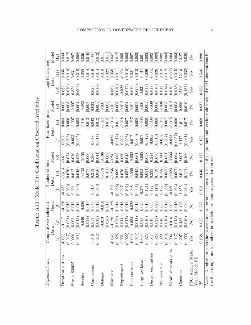
COMPETITION IN GOVERNMENT PROCUREMENT 79
TableA10.
Model
Fit
:C
ondit
ional
onO
bse
rved
Att
ribute
s
Dep
enden
tva
r.C
omp
etit
ivel
yso
lici
ted
Nu
mb
erof
bid
sF
irm
-fixed
-pri
ceL
og(F
inal
pri
ce)
Dat
aM
od
elD
ata
Mod
elD
ata
Mod
elD
ata
Mod
el(1
)(2
)(3
)(4
)(5
)(6
)(7
)(8
)(9
)(1
0)
(11)
(12)
Du
rati
on>
3m
o.-0
.083
-0.1
17-0
.120
-0.5
32
-0.6
14
-0.6
11
0.0
02
0.0
03
0.0
05
0.0
32
0.0
35
0.0
34
(0.0
17)
(0.0
21)
[0.0
15]
(0.0
63)
(0.0
70)
[0.0
74]
(0.0
06)
(0.0
06)
[0.0
03]
(0.0
10)
(0.0
10)
[0.0
12]
Siz
e>
$300
K0.
0001
0.00
30.
013
0.0
04
0.0
17
0.0
36
-0.0
05
-0.0
07
-0.0
07
0.8
29
0.8
31
0.8
07
(0.0
11)
(0.0
13)
[0.0
14]
(0.0
49)
(0.0
48)
[0.0
58]
(0.0
05)
(0.0
05)
[0.0
04]
(0.0
09)
(0.0
10)
[0.0
08]
Ser
vic
e-0
.046
-0.0
26-0
.152
-0.1
55
-0.1
01
-0.0
82
0.0
55
0.0
36
(0.0
24)
[0.0
19]
(0.0
77)
[0.0
60]
(0.0
12)
[0.0
07]
(0.0
14)
[0.0
16]
Com
mer
cial
0.04
60.
053
0.04
50.3
10
0.3
12
0.3
06
0.0
48
0.0
43
0.0
32
0.0
25
0.0
19
-0.0
04
(0.0
12)
(0.0
12)
[0.0
12]
(0.0
43)
(0.0
50)
[0.0
41]
(0.0
14)
(0.0
12)
[0.0
05]
(0.0
18)
(0.0
14)
[0.0
12]
Def
ense
-0.0
13-0
.010
-0.1
78
-0.1
98
-0.0
11
-0.0
07
0.0
10
0.0
11
(0.0
20)
[0.0
17]
(0.1
01)
[0.0
67]
(0.0
15)
[0.0
05]
(0.0
22)
[0.0
11]
Com
ple
x-0
.045
-0.1
28-0
.129
-0.1
73
-0.2
66
-0.2
41
-0.0
25
-0.0
14
-0.0
11
0.0
62
0.0
58
0.0
47
(0.0
25)
(0.0
26)
[0.0
14]
(0.0
58)
(0.0
69)
[0.0
63]
(0.0
12)
(0.0
11)
[0.0
05]
(0.0
10)
(0.0
11)
[0.0
12]
Exp
erie
nce
d0.
061
0.01
40.
018
0.0
37
0.0
76
0.0
80
0.0
02
-0.0
18
-0.0
12
-0.0
22
-0.0
04
0.0
05
(0.0
22)
(0.0
17)
[0.0
14]
(0.1
01)
(0.0
52)
[0.0
48]
(0.0
08)
(0.0
07)
[0.0
04]
(0.0
12)
(0.0
10)
[0.0
03]
Pas
tco
ntr
act
-0.0
04-0
.024
-0.0
280.0
08
-0.0
69
-0.0
52
-0.0
17
-0.0
17
-0.0
11
0.0
19
0.0
21
0.0
07
(0.0
14)
(0.0
14)
[0.0
14]
(0.0
41)
(0.0
45)
[0.0
61]
(0.0
09)
(0.0
08)
[0.0
05]
(0.0
09)
(0.0
10)
[0.0
03]
Lar
gew
orklo
ad-0
.006
0.02
30.
023
-0.2
70
0.0
03
-0.0
05
-0.0
07
-0.0
03
-0.0
01
-0.0
21
-0.0
15
0.0
01
(0.0
25)
(0.0
16)
[0.0
13]
(0.1
21)
(0.0
54)
[0.0
58]
(0.0
12)
(0.0
09)
[0.0
05]
(0.0
13)
(0.0
09)
[0.0
02]
Bu
dge
tco
mm
itte
e0.
047
0.04
60.
053
0.1
77
0.2
33
0.2
14
-0.0
05
-0.0
08
-0.0
09
0.0
18
-0.0
02
0.0
02
(0.0
25)
(0.0
29)
[0.0
20]
(0.1
18)
(0.1
19)
[0.0
76]
(0.0
10)
(0.0
08)
[0.0
06]
(0.0
19)
(0.0
26)
[0.0
03]
Win
ner
s≥
20.
020
0.04
60.
035
0.1
27
0.1
58
0.1
41
-0.0
15
-0.0
11
-0.0
06
0.0
12
0.0
10
0.0
02
(0.0
19)
(0.0
16)
[0.0
16]
(0.0
58)
(0.0
57)
[0.0
51]
(0.0
07)
(0.0
07)
[0.0
05]
(0.0
14)
(0.0
12)
[0.0
03]
Est
abli
shm
ents≥
240.
004
-0.0
160.
009
-0.0
30
-0.0
23
-0.0
33
-0.0
23
-0.0
15
-0.0
12
0.0
10
-0.0
00
0.0
04
(0.0
17)
(0.0
13)
[0.0
18]
(0.0
63)
(0.0
07)
[0.0
64]
(0.0
057)
(0.0
06)
[0.0
03]
(0.0
18)
(0.0
15)
[0.0
03]
Con
stan
t0.
207
0.43
30.4
261.8
56
2.0
12
2.0
07
1.1
75
1.0
11
0.9
96
12.0
612.1
612.2
7(0
.060
)(0
.040
)[0
.030
](0
.284)
(0.1
11)
[0.1
66]
(0.0
31)
(0.0
17)
[0.0
10]
(0.1
32)
(0.0
32)
[0.0
20]
PS
C,
Age
ncy
,S
tate
,Y
esN
oN
oY
esN
oN
oY
esN
oN
oY
esN
oN
oY
ear,
Mon
thF
ER
20.
158
0.05
20.2
750.1
31
0.0
48
0.1
72
0.1
25
0.0
69
0.6
37
0.5
58
0.5
46
0.9
98
Note
s:N
um
ber
sin
par
enth
eses
are
stan
dar
der
rors
clu
ster
edat
the
4-d
igit
pro
du
ctan
dse
rvic
eco
de
leve
l;all
6,9
81
ob
serv
ati
on
sin
the
fin
alsa
mp
leu
sed
;num
ber
sin
bra
cket
sar
eb
oots
trap
stan
dard
erro
rs.
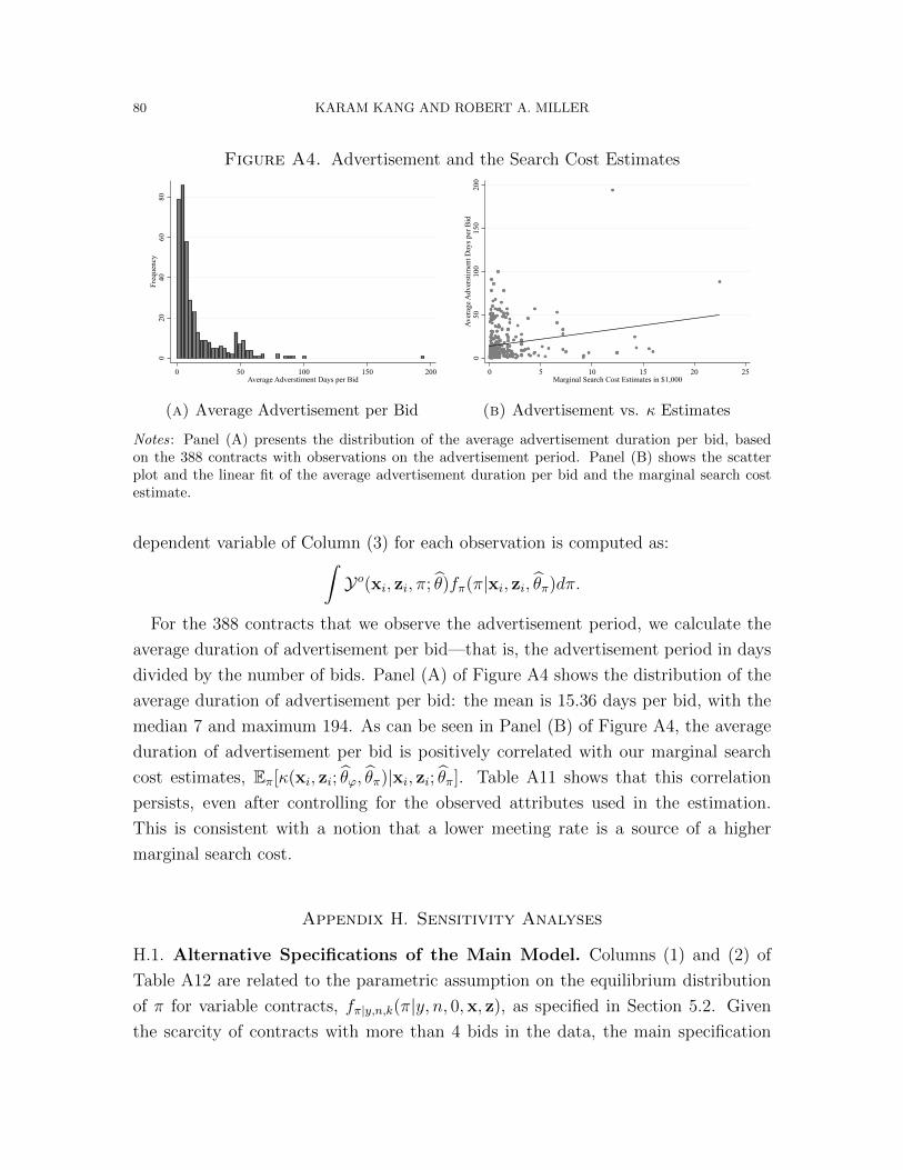
80 KARAM KANG AND ROBERT A. MILLER
Figure A4. Advertisement and the Search Cost Estimates0
20
40
60
80
Fre
quen
cy
0 50 100 150 200Average Adverstiment Days per Bid
(a) Average Advertisement per Bid
050
100
150
200
Aver
age
Adver
stim
ent
Day
s per
Bid
0 5 10 15 20 25Marginal Search Cost Estimates in $1,000
(b) Advertisement vs. κ Estimates
Notes: Panel (A) presents the distribution of the average advertisement duration per bid, basedon the 388 contracts with observations on the advertisement period. Panel (B) shows the scatterplot and the linear fit of the average advertisement duration per bid and the marginal search costestimate.
dependent variable of Column (3) for each observation is computed as:∫Yo(xi, zi, π; θ)fπ(π|xi, zi, θπ)dπ.
For the 388 contracts that we observe the advertisement period, we calculate the
average duration of advertisement per bid—that is, the advertisement period in days
divided by the number of bids. Panel (A) of Figure A4 shows the distribution of the
average duration of advertisement per bid: the mean is 15.36 days per bid, with the
median 7 and maximum 194. As can be seen in Panel (B) of Figure A4, the average
duration of advertisement per bid is positively correlated with our marginal search
cost estimates, Eπ[κ(xi, zi; θϕ, θπ)|xi, zi; θπ]. Table A11 shows that this correlation
persists, even after controlling for the observed attributes used in the estimation.
This is consistent with a notion that a lower meeting rate is a source of a higher
marginal search cost.
Appendix H. Sensitivity Analyses
H.1. Alternative Specifications of the Main Model. Columns (1) and (2) of
Table A12 are related to the parametric assumption on the equilibrium distribution
of π for variable contracts, fπ|y,n,k(π|y, n, 0,x, z), as specified in Section 5.2. Given
the scarcity of contracts with more than 4 bids in the data, the main specification
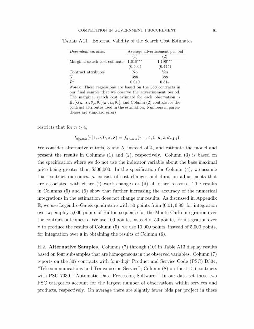
COMPETITION IN GOVERNMENT PROCUREMENT 81
Table A11. External Validity of the Search Cost Estimates
Dependent variable: Average advertisement per bid(1) (2)
Marginal search cost estimate 1.618∗∗∗ 1.196∗∗∗
(0.404) (0.445)
Contract attributes No YesN 388 388R2 0.040 0.314Notes: These regressions are based on the 388 contracts inour final sample that we observe the advertisement period.The marginal search cost estimate for each observation is
Eπ[κ(xi, zi; θϕ, θπ)|xi, zi; θπ], and Column (2) controls for thecontract attributes used in the estimation. Numbers in paren-theses are standard errors.
restricts that for n > 4,
fπ|y,n,k(π|1, n, 0,x, z) = fπ|y,n,k(π|1, 4, 0,x, z; θπ,1,4).
We consider alternative cutoffs, 3 and 5, instead of 4, and estimate the model and
present the results in Columns (1) and (2), respectively. Column (3) is based on
the specification where we do not use the indicator variable about the base maximal
price being greater than $300,000. In the specification for Column (4), we assume
that contract outcomes, s, consist of cost changes and duration adjustments that
are associated with either (i) work changes or (ii) all other reasons. The results
in Columns (5) and (6) show that further increasing the accuracy of the numerical
integrations in the estimation does not change our results. As discussed in Appendix
E, we use Legendre-Gauss quadrature with 50 points from [0.01, 0.99] for integration
over π; employ 5,000 points of Halton sequence for the Monte-Carlo integration over
the contract outcomes s. We use 100 points, instead of 50 points, for integration over
π to produce the results of Column (5); we use 10,000 points, instead of 5,000 points,
for integration over s in obtaining the results of Column (6).
H.2. Alternative Samples. Columns (7) through (10) in Table A13 display results
based on four subsamples that are homogeneous in the observed variables. Column (7)
reports on the 307 contracts with four-digit Product and Service Code (PSC) D304,
“Telecommunications and Transmission Service”; Column (8) on the 1,156 contracts
with PSC 7030, “Automatic Data Processing Software.” In our data set these two
PSC categories account for the largest number of observations within services and
products, respectively. On average there are slightly fewer bids per project in these
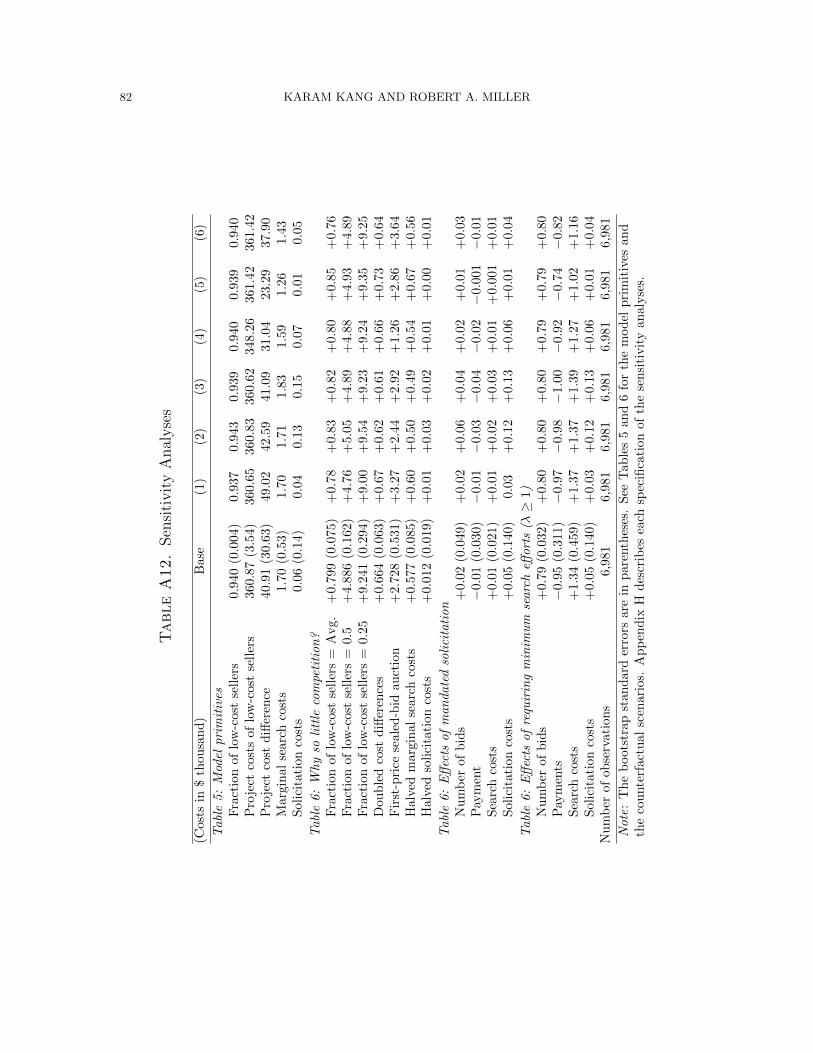
82 KARAM KANG AND ROBERT A. MILLER
TableA12.
Sen
siti
vit
yA
nal
yse
s
(Cos
tsin
$th
ousa
nd
)B
ase
(1)
(2)
(3)
(4)
(5)
(6)
Tabl
e5:
Mod
elpri
mit
ives
Fra
ctio
nof
low
-cos
tse
ller
s0.9
40
(0.0
04)
0.9
37
0.9
43
0.9
39
0.9
40
0.9
39
0.9
40
Pro
ject
cost
sof
low
-cos
tse
ller
s360.8
7(3
.54)
360.6
5360.8
3360.6
2348.2
6361.4
2361.4
2P
roje
ctco
std
iffer
ence
40.9
1(3
0.6
3)
49.0
242.5
941.0
931.0
423.2
937.9
0M
argi
nal
sear
chco
sts
1.7
0(0
.53)
1.7
01.7
11.8
31.5
91.2
61.4
3S
olic
itat
ion
cost
s0.0
6(0
.14)
0.0
40.1
30.1
50.0
70.0
10.0
5
Tabl
e6:
Why
soli
ttle
com
peti
tion
?F
ract
ion
oflo
w-c
ost
sell
ers
=A
vg.
+0.7
99
(0.0
75)
+0.7
8+
0.8
3+
0.8
2+
0.8
0+
0.8
5+
0.7
6F
ract
ion
oflo
w-c
ost
sell
ers
=0.5
+4.8
86
(0.1
62)
+4.7
6+
5.0
5+
4.8
9+
4.8
8+
4.9
3+
4.8
9F
ract
ion
oflo
w-c
ost
sell
ers
=0.2
5+
9.2
41
(0.2
94)
+9.0
0+
9.5
4+
9.2
3+
9.2
4+
9.3
5+
9.2
5D
oub
led
cost
diff
eren
ces
+0.6
64
(0.0
63)
+0.6
7+
0.6
2+
0.6
1+
0.6
6+
0.7
3+
0.6
4F
irst
-pri
cese
aled
-bid
auct
ion
+2.7
28
(0.5
31)
+3.2
7+
2.4
4+
2.9
2+
1.2
6+
2.8
6+
3.6
4H
alve
dm
argi
nal
sear
chco
sts
+0.5
77
(0.0
85)
+0.6
0+
0.5
0+
0.4
9+
0.5
4+
0.6
7+
0.5
6H
alve
dso
lici
tati
onco
sts
+0.0
12
(0.0
19)
+0.0
1+
0.0
3+
0.0
2+
0.0
1+
0.0
0+
0.0
1
Tabl
e6:
Eff
ects
of
man
date
dso
lici
tati
on
Nu
mb
erof
bid
s+
0.0
2(0
.049)
+0.0
2+
0.0
6+
0.0
4+
0.0
2+
0.0
1+
0.0
3P
aym
ent
−0.0
1(0
.030)−
0.0
1−
0.0
3−
0.0
4−
0.0
2−
0.0
01−
0.0
1S
earc
hco
sts
+0.0
1(0
.021)
+0.0
1+
0.0
2+
0.0
3+
0.0
1+
0.0
01
+0.0
1S
olic
itat
ion
cost
s+
0.0
5(0
.140)
0.0
3+
0.1
2+
0.1
3+
0.0
6+
0.0
1+
0.0
4
Tabl
e6:
Eff
ects
of
requ
irin
gm
inim
um
searc
heff
ort
s(λ≥
1)
Nu
mb
erof
bid
s+
0.7
9(0
.032)
+0.8
0+
0.8
0+
0.8
0+
0.7
9+
0.7
9+
0.8
0P
aym
ents
−0.9
5(0
.311)−
0.9
7−
0.9
8−
1.0
0−
0.9
2−
0.7
4−
0.8
2S
earc
hco
sts
+1.3
4(0
.459)
+1.3
7+
1.3
7+
1.3
9+
1.2
7+
1.0
2+
1.1
6S
olic
itat
ion
cost
s+
0.0
5(0
.140)
+0.0
3+
0.1
2+
0.1
3+
0.0
6+
0.0
1+
0.0
4N
um
ber
ofob
serv
atio
ns
6,9
81
6,9
81
6,9
81
6,9
81
6,9
81
6,9
81
6,9
81
Note
:T
he
boot
stra
pst
and
ard
erro
rsare
inp
are
nth
eses
.S
eeT
ab
les
5an
d6
for
the
mod
elp
rim
itiv
esan
dth
eco
unte
rfac
tual
scen
ario
s.A
pp
end
ixH
des
crib
esea
chsp
ecifi
cati
on
of
the
sen
siti
vit
yan
aly
ses.
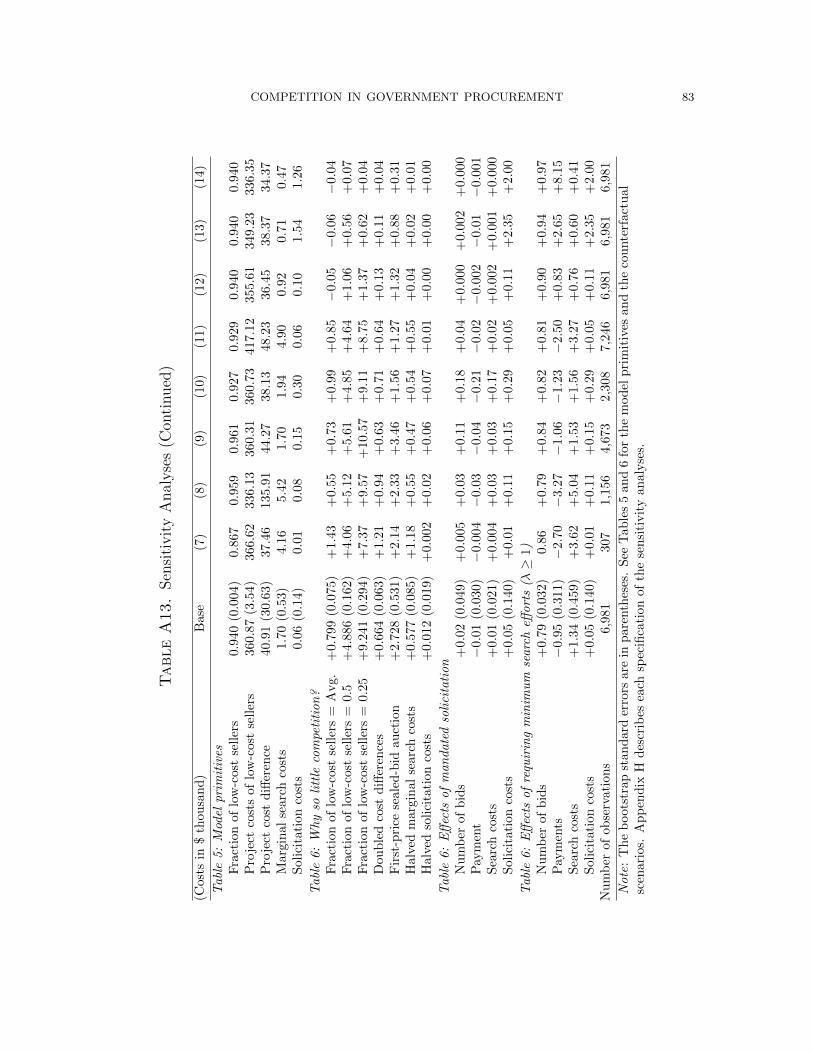
COMPETITION IN GOVERNMENT PROCUREMENT 83
TableA13.
Sen
siti
vit
yA
nal
yse
s(C
onti
nued
)
(Cos
tsin
$th
ousa
nd
)B
ase
(7)
(8)
(9)
(10)
(11)
(12)
(13)
(14)
Tabl
e5:
Mod
elpri
mit
ives
Fra
ctio
nof
low
-cos
tse
ller
s0.9
40
(0.0
04)
0.8
67
0.9
59
0.9
61
0.9
27
0.9
29
0.9
40
0.9
40
0.9
40
Pro
ject
cost
sof
low
-cos
tse
ller
s360.8
7(3
.54)
366.6
2336.1
3360.3
1360.7
3417.1
2355.6
1349.2
3336.3
5P
roje
ctco
std
iffer
ence
40.9
1(3
0.6
3)
37.4
6135.9
144.2
738.1
348.2
336.4
538.3
734.3
7M
argi
nal
sear
chco
sts
1.7
0(0
.53)
4.1
65.4
21.7
01.9
44.9
00.9
20.7
10.4
7S
olic
itat
ion
cost
s0.0
6(0
.14)
0.0
10.0
80.1
50.3
00.0
60.1
01.5
41.2
6
Tabl
e6:
Why
soli
ttle
com
peti
tion
?F
ract
ion
oflo
w-c
ost
sell
ers
=A
vg.
+0.7
99
(0.0
75)
+1.4
3+
0.5
5+
0.7
3+
0.9
9+
0.8
5−
0.0
5−
0.0
6−
0.0
4F
ract
ion
oflo
w-c
ost
sell
ers
=0.
5+
4.8
86
(0.1
62)
+4.0
6+
5.1
2+
5.6
1+
4.8
5+
4.6
4+
1.0
6+
0.5
6+
0.0
7F
ract
ion
oflo
w-c
ost
sell
ers
=0.
25+
9.2
41
(0.2
94)
+7.3
7+
9.5
7+
10.5
7+
9.1
1+
8.7
5+
1.3
7+
0.6
2+
0.0
4D
oub
led
cost
diff
eren
ces
+0.6
64
(0.0
63)
+1.2
1+
0.9
4+
0.6
3+
0.7
1+
0.6
4+
0.1
3+
0.1
1+
0.0
4F
irst
-pri
cese
aled
-bid
auct
ion
+2.7
28
(0.5
31)
+2.1
4+
2.3
3+
3.4
6+
1.5
6+
1.2
7+
1.3
2+
0.8
8+
0.3
1H
alve
dm
argi
nal
sear
chco
sts
+0.5
77
(0.0
85)
+1.1
8+
0.5
5+
0.4
7+
0.5
4+
0.5
5+
0.0
4+
0.0
2+
0.0
1H
alve
dso
lici
tati
onco
sts
+0.0
12
(0.0
19)
+0.0
02
+0.0
2+
0.0
6+
0.0
7+
0.0
1+
0.0
0+
0.0
0+
0.0
0
Tabl
e6:
Eff
ects
of
ma
ndate
dso
lici
tati
on
Nu
mb
erof
bid
s+
0.0
2(0
.049)
+0.0
05
+0.0
3+
0.1
1+
0.1
8+
0.0
4+
0.0
00
+0.0
02
+0.0
00
Pay
men
t−
0.0
1(0
.030)−
0.0
04−
0.0
3−
0.0
4−
0.2
1−
0.0
2−
0.0
02−
0.0
1−
0.0
01
Sea
rch
cost
s+
0.0
1(0
.021)
+0.0
04
+0.0
3+
0.0
3+
0.1
7+
0.0
2+
0.0
02
+0.0
01
+0.0
00
Sol
icit
atio
nco
sts
+0.0
5(0
.140)
+0.0
1+
0.1
1+
0.1
5+
0.2
9+
0.0
5+
0.1
1+
2.3
5+
2.0
0
Tabl
e6:
Eff
ects
of
requ
irin
gm
inim
um
searc
heff
ort
s(λ≥
1)N
um
ber
ofb
ids
+0.7
9(0
.032)
0.8
6+
0.7
9+
0.8
4+
0.8
2+
0.8
1+
0.9
0+
0.9
4+
0.9
7P
aym
ents
−0.9
5(0
.311)−
2.7
0−
3.2
7−
1.0
6−
1.2
3−
2.5
0+
0.8
3+
2.6
5+
8.1
5S
earc
hco
sts
+1.3
4(0
.459)
+3.6
2+
5.0
4+
1.5
3+
1.5
6+
3.2
7+
0.7
6+
0.6
0+
0.4
1S
olic
itat
ion
cost
s+
0.0
5(0
.140)
+0.0
1+
0.1
1+
0.1
5+
0.2
9+
0.0
5+
0.1
1+
2.3
5+
2.0
0N
um
ber
ofob
serv
atio
ns
6,9
81
307
1,1
56
4,6
73
2,3
08
7,2
46
6,9
81
6,9
81
6,9
81
Note
:T
he
boot
stra
pst
and
ard
erro
rsar
ein
pare
nth
eses
.S
eeT
ab
les
5an
d6
for
the
mod
elp
rim
itiv
esan
dth
eco
unte
rfact
ual
scen
ario
s.A
pp
end
ixH
des
crib
esea
chsp
ecifi
cati
on
of
the
sensi
tivit
yan
aly
ses.
84 KARAM KANG AND ROBERT A. MILLER
subsamples, 1.31 and 1.60 respectively, than overall, 1.64. Comparing Columns (7)
and (8), we find a larger pool of high-cost sellers and smaller project cost differ-
ences between the two seller types for the telecommunications/transmission service
contracts than for the software contracts. Comparing these two subsamples with the
main sample, the roles of seller heterogeneity and buyer search costs in explaining few
bids differ somewhat, but the results are qualitatively similar across all three samples.
Instead of pooling the Department of Defense (DoD) contracts and others as in our
main estimation, we separately estimate the model using the 4,673 DoD contracts
only for the results of Column (9), and use the remainders only for Column (10).
Column (11) is based on our main sample plus the 265 contracts that we originally
dropped due to inconsistent records in terms of price and duration (Appendix A.2).
Our results in Section 6 are robust to using these alternative samples.
H.3. Allowing for Entry Costs. For Columns (12)–(14), we consider an extended
model where sellers pay entry costs to participate, as discussed in Section 3.4. We
assume that the entry cost per seller is a fraction of the expected project cost:
κs(x1, π; θϕ) = ακ [πc1(x1, π; θϕ) + (1− π)c0(x1, π; θϕ)] .
Borrowing the estimates from the literature, we set ακ = 0.01, 0.02, 0.05, respec-
tively. As we allow for another source of market friction, the estimates of marginal
search costs are smaller and mean solicitation costs are larger than the main esti-
mates. Regardless, we find that the effects of mandating more competition are very
similar, except that requiring minimum search efforts (λ ≥ 1) would increase the
expected payment. It is because the buyer would have to increase the amount of the
reimbursement of entry costs to be included in the payment to a winning seller in
order to induce sellers to participate when they expect more bids.
H.3.1. Equilibrium when Sellers Pay Entry Costs. We assume that sellers do not
know their cost type before entry. Upon paying the entry cost, they learn their type.
Assuming the sellers’ belief on their type is based on the population distribution, the
reimbursement of the entry cost to the winner, denoted as a, must be a fair lottery
COMPETITION IN GOVERNMENT PROCUREMENT 85
given the buyer’s search intensity λ > 0:
κs = a
∞∑j=0
[πφ1,j+1 + (1− π)φ0,j+1]λje−λ
j!
= a∞∑j=0
[π
1− (1− π)(j+1)
(j + 1)π+ (1− π)
(1− π)j
j + 1
]λje−λ
j!
= a
∞∑j=0
1
j + 1
λje−λ
j!=a
λ
∞∑j=0
λj+1e−λ
(j + 1)!=a
λ
∞∑j′=1
λj′e−λ
j′!=a
λ(1− e−λ),
where the second equality results from plugging in the definitions of φ1n and φ0n, (5)
and (6). Therefore, the reimbursement to the winner is κsλ/(1− e−λ) if λ > 0 and κs
otherwise. The expected payment to a winning seller when there are n participants
under search intensity λ, denoted by T e(n), is:
T e(n) = T (n) + κs
(1λ>0
λ
1− e−λ+ 1λ=0
),
where T (n) is defined in (12). The expected total cost of competitive procurement
with search effort λ and solicitation costs η, denoted by U e(λ, η), is:
U e(λ, η) ≡∞∑n=0
λne−λ
n!T e(n+ 1) + κλ+ η = U(λ, η) + κs
(1λ>0
λ
1− e−λ+ 1λ=0
),
where U(λ, η) is defined in (16). If the optimal search intensity conditional on com-
petition, denoted by λe, is positive, then it must satisfy the first order condition:
−πe−λπ
(1− π)(c0 − c1) + π(γ0 − γ1) + Γ
+ κs
(1
1− e−λ− λe−λ
(1− e−λ)2
)+ κ = 0.
Denoting the root to the above equation by λ, λe = max0, λ. There is competitive
bidding if and only if U e(λe, η) ≤ U(0, 0), or equivalently, η ≤ Ωe, where
Ωe = Ω + κs1λe>0[1− λe/(1− e−λe)
],
where Ω is defined in (17).
H.3.2. Estimation when Sellers Pay Entry Costs. The estimation procedures of E.1
are identical to the estimation of the model when κs = 0. In addition, because the
equilibrium search intensity estimates are based on θπ, λe(π, x, θπ) is also the same as
the estimates from the main specification. In implementing E.2, we use the following
86 KARAM KANG AND ROBERT A. MILLER
identities:
E[p|y, n, k = 1, x] =
∫ [p1n(x1, π; θϕ) + κs(x1, π; θϕ)
(1λe(π,x;θπ)>0
λe(π, x; θπ)
1− e−λe(π,x;θπ)
+1λe(π,x;θπ)=0
)]fπ|y,n,k(π|y, n, 1, x; θπ)dπ,
E[p|y, n, k = 1, x] =
∫ [p0(x1, π; θϕ) + κs(x1, π; θϕ)
(1λe(π,x;θπ)>0
λe(π, x; θπ)
1− e−λe(π,x;θπ)
+1λe(π,x;θπ)=0
)]fπ|y,n,k(π|y, n, 1, x; θπ)dπ,
E[q|y, n, k = 0, s, x] =
∫q0(s,x, π; θϕ)fπ|y,n,k(π|y, n, 0, x; θπ)dπ,
where p1n(x, π; θr), p0(x, π; θr), and q0(s,x, π; θr) are defined in (A.33). Given these
identities, similarly estimate θϕ2 , a subset of θϕ, by minimizing the weighted sum of
squared distances from the predicted and the actual values of the base prices and
the price adjustments. In implementing E.3, the estimates of κ(x, π; θ∗ϕ, θ∗π) and
Ωe(x, π; θ∗ϕ, θ∗π) are modified to:
κ(x, π; θϕ, θπ) = πe−πλe(π,x;θπ)
[πγ0(x1, π; θc)− γ1(x1, π; θc)
+(1− π)
c0(x1, π; θϕ)− c1(x1, π; θϕ)
+ Γ(x1, π; θϕ)
]−κs(x1, π; θϕ)1λe(π,x;θπ)>0
(1− e−λe(π,x;θπ)[1 + λe(π, x; θπ)]
[1− e−λe(π,x;θπ)]2
),
and
Ωe(x, π; θϕ, θπ) = Ω(x, π; θϕ, θπ) + κs(x1, π; θϕ)1λe(π,x;θπ)>0
(1− λe(π, x; θπ)
1− e−λe(π,x;θπ)
).