Stream gaging by continuous injection of tracer elements

Item Type Thesis-Reproduction (electronic); text

Authors Werrell, William Lewis,1931-

Publisher The University of Arizona.

Rights Copyright © is held by the author. Digital access to this materialis made possible by the University Libraries, University of Arizona.Further transmission, reproduction or presentation (such aspublic display or performance) of protected items is prohibitedexcept with permission of the author.

Download date 29/05/2018 10:19:06

Link to Item http://hdl.handle.net/10150/191479

STREAM GAGING BY CONT]UOUS INJECTION

OF TRACER ELEMENTS

by

William Lewis Werrell

A Thesis Submitted to the Faculty of the

GRADUATE COMMITTEE ON HYDROLOGY

In Partial Fulfillment of the RequirementsFor the Degree of

MASTER OF SCIENCE

In the Graduate College

THE UNIVERSITY OF ARIZONA

1967

This thesis has been submitted in partial fulfillment of require-ments for an advanced degree at The University of Arizona and isdeposited in the University Library to be made available to borrowersunder rules of the library.

Brief quotations from this thesis are allowable without specialpermission, provided that accurate acknowledgment of source is made.Requests for permission for extended quotation from or reproduction ofthis manuscript in whole or in part may be granted by the head of themajor department or the Dean of the Graduate College when in hisjudgment the proposed use of the material is in the interests of scholarS-ship. In all other instances, however, permission must be obtainedfrom the author.

E

STATEMENT BY AUTHOR

SIGNED:

APPROVAL BY THESIS DIRECTOR

This thesis has been approved on the date shown below:

ENE S. SIMPPr essor of Hydrology

c%7

ACKNOWLEDGMENTS

The author wishes to thank Dr. E. S. Simpson, who suggested

the thesis topic and directed the study. Acknowledgment also is given

to Mr. Dallas Childers, who conducted the current-meter measure-

ments on the discharge of Sabtho Creek. Thanks are given to the

following individuals, who accompanied me on field trips and served

as sample collectors: my wife, Robin; Mr. and Mrs. Jack Edmonds;

Mr. Stuart Brown; Mr. Robert Lichty; and Mr. Raymond Harshbarger.

111

TABLE OF CONTENTS

Page

LIST OF ILLUSTRATIONS vi

LIST OF TABLES vii

ABSTRACT viii

INTRODUCTION 1

TRACER-DILUTION METHOD OF DETERMININGSTREAM DISCHARGE 5

Introduction 5

Tracers 8

Fluorescein Dye-Dilution Method 10

Dye Solutions 10Background Fluorescence 12Computation of Stream Discharge 13Dye Injection 15

Mariotte-Flask Method 16Floating-Syphon Method 19Constant-Head Tank Method 19

A Review of Mixing Length and Dispersion Equations 20Dye Samples Collected 23Fluorometer Operating Procedure 24

Laboratory Experiments 30

Matching of Cuvettes 30Fluorescence Loss Due to Direct Sunlight 32

iv

TABLE OF CONTENTS Continued

V

Page

Field Experiments 38

Willow Creek Test 39Sabino Creek Test 46Paria River Test 51

Chinle Wash Test 55

DISCUSSION AND SUMMARY 58

Possible Sources of Error 58Future Uses 60Future Developments 63Conclusion 63

APPENDIX AWILLOW CREEK TEST 65

APPENDIX BSABINO CREEK TEST 73

APPENDIX CPARIA RIVER TEST 76

APPENDIX DCHINLE WASH TEST 81

REFERENCES 84

LIST OF ILLUSTRATIONS

Page

Figure

Mariotte flask, principle of operation 17

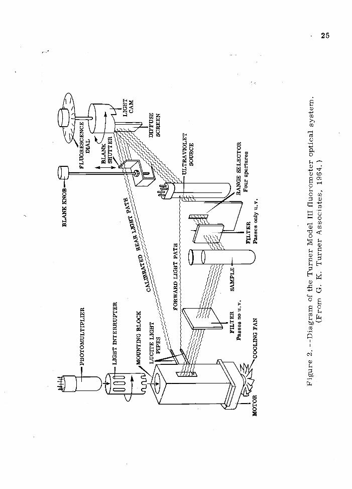
Diagram of the Turner Model IIIfluorometer optical system 25

Variation of fluorescence withexposure to sunlight 34

Decay of Brilliant Pontacyl Pink B onexposure to direct sunlight 36

Flow in Willow Creek 41

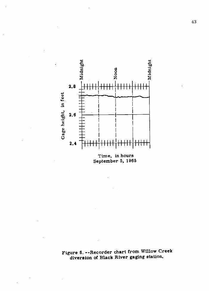
Recorder chart from Willow Creek diversionof Black River gaging station 43

Recorder chart from Sabino Creek gaging station 48

Flow in Sabino Creek 49

Dye injection at the upper end of the PariaRiver test reach 52

Recorder chart from Paria River gaging station 53

Recorder chart from Chinle Wash gaging station 56

vi

LIST OF TABLES

Page

Table

1. Discharge computations for Sabino Creekbased on U. S. Geological Survey gaging-station record and dye-dilution measurement 50

vii

STREAM GAGING BY CONTINUOUS INJECTIONOF TRACER ELEMENTS

By

William Lewis Werrell

ABSTRACT

The practical application of the use of fluorescent-dye tracer

elements as a means of determining stream discharge was the con-

sideration of this study. Although this approach is not new in princi-

ple, recent developments in fluorometry and the development of new

and less expensive fluorescent dyes warrant reappraisal of the

method,

During this study, the proper use of the fluorometer was

mastered, properties of the dye were examined by laboratory tests,

and four field tests were conducted. Three of the field tests allowed

direct comparison between discharge computed by the dye-dilution

method and discharge measured by a current meter; the maximum

variation between the results of these tests was 11 percent.

viii

ix

The dye-dilution method may be used on streams in the South-

west for high-water measurements of flow above wading stage where

no cableway is present or where no adequate current-meter measure-

ment section can be found. The possibility of future automation of

this measurement system holds promise for the rating of new gaging

stations and for providing streamfiow records in remote areas.

INTRODUCTION

The semiarid and desert regions of the United States present

special problems in the determination of the factors included in a

water budget surface-water inflow, outflow, evapotranspiration, etc.

In these regions, efficient utilization of the available water resources

is of utmost importance in order to maintain even the present degree

of water usage. In addition, the predicted rapid population growth will

further tax the water resources.

The importance of surface water cannot be overestimated.

Flowing streams offer the most accessible and often the most economic

water supply for mants use. Streams maintain lakes and ponds for

recreation and sustain the areats natural wildlife. Influent streams

are the major source of ground-water recharge in areas of rapid

ground-water decline. However, sediment problems are inherently

connected with streamflow.

In the semiarid Southwest, streams that have small drainage

areas flow intermittently, perhaps only two or three times a year in

response to local rainfall; however, when precipitation does occur, a

substantial part of the total runoff for the year may occur within a few

1

2

hours. Steep stream gradients and the lack of vegetative cover allow

rapid runoff. Rainstorms generate streamfiow in which the rising

limb of the hydrograph is characteristically steep, and the recession

to zero flow may occur within minutes or hours.

As the need for accurate data for scientific water management

becomes more critical, new methods for obtaining these data must be

developed. The provision of these data, in a large part, is the respon-

sibility of the U. S. Geological Survey. In order to obtain these data,

surface-water gaging stations have been established throughout the

Southwest. New stations constantly are being added to the existing pro-

gram. In many places, these stations, by necessity, are established

along sand-channel streambeds on alluvial plains. The establishment

of the stage-discharge relations for these stations is difficult, time

consuming, and never-ending. Discharge ratings for sand-channel

streams are shifting continually, as the controlling section of the river

changes. In many instances, it is difficult or impossible to measure

the discharge by current-meter methods without a bridge or cableway,

because the force of the current is too strong to permit wading. Some

stations are not easily accessible, and often there is no flood warning

because of their location in sparsely populated areas.

Present methods for the continuous determination of stream

discharge are based on a stage-discharge relation, in which gage

height, the independent variable, is determined by one of two types of

3

gagesrecording or nonrecording. Recording gages are necessary to

record the stage-time relation, which is used with the stage-discharge

relation to determine discharge. Stage recorders are either short- or

long-term-7-day or continuousand are of the analog or digital type.

Nonrecording gages used to measure stage are the staff, wire-weight,

tape-weight, chain-weight, float, electric, hook, and pressure gages,

which may be used alone or in conjunction with continuous recorders.

The stage-discharge relation is determined by measuring the dis-

charge, at different stages, with a current meter or through computa-

tions using indirect methods.

Factors that affect the stage-discharge relations for individual

streams are scour and fill of the streambed, streambed regime, vari-

able slope, ice, aquatic vegetation, debris on the control, and changes

in velocity and direction of the current.

Indirect measurements used to determine the instantaneous

peak discharge are the slope area (application of the Bernoulli energy

equation) and flow through contracted openings, culverts, over roadway

embankments, and over dams, The crest-stage gage, which measures

only the peak stage of a particular flow, is often used to assist with

indirect measurements.

The extremely short periods of flow, the scour-on-rise and

fill-on-recession characteristics of sand-channel streams, the diffi-

culty of making current-meter measurements, and the inaccessibility

4

of stations that have no flood-warning system present serious difficul-

ties in collecting surface-water data in the Southwest and other arid or

semiarid regions. Stream gaging by continuous injection and monitor-

ing of tracer elements shows promise in overcoming many of these

difficulties.

TRACER-DILUTION METHOD OF DETERMININGSTREAM DISCHARGE

Introduction

The tracer-dilution method of determining stream discharge

consists of injecting a highly concentrated but small quantity of tracer

solution of known or determinable strength into streamfiow. After

release, the fluid is allowed to flow downstream for a distance, so that

it will become homogeneously, vertically, and laterally dispersed

throughout the stream cross section. Monitoring of the tracer is con-

ducted downstream from this point. By determining the amount of

tracer dilution, the quantity of flow can be computed, if it can be as-

sumed that no loss or gain of the tracer occurred during the test.

Discharge computed by the dye-dilution method is the quantity

of flow occurring at the point where homogeneous mixing of the dye

takes place. Assuming that there is no loss or gain of dye during the

test and that the stream is not influent, valid sampling may be conduct-

ed at any point downstream. Thus, for the rating of a gaging station,

the dye-dilution test must be located so that mtxing will occur up-

stream from the gaging station; sampling should be conducted at the

5

6

station if possible. If additional water is added to the stream, such as

tributary inflow, sampling must be done at some distance downstream,

the distance being sufficient so that the dye will become homogeneously

mixed with the total or combined flow.

The cross-sectional area of the channel and the stream veloc-

ities are not necessary to determine discharge by the dye-dilution

method, which is a great advantage. This eliminates the necessity of

wading the stream or, during high flow, the need for a cable car. The

dye-dilution method can be used in most reaches of the stream channel

without regard for the usual factors that must be considered in proper

selection of a current-meter measurement section or the factors that

affect the choice of sections for a slope-area measurementchannel

roughness, velocity direction, and straightness of channel.

At typical sand-channel gaging stations, the computation of

the stage-time records requires the use of adjustment or shift curves

due to scour-fill conditions in the channel. Between current-meter

measurements, the proper adjustment of the stage record may be high-

ly speculative. The dye-injection method of computing flow eliminates

this problem. Future development of a continuous sampling apparatus

will allow complete automation of the dye-dilution method of determin-

ing stream discharge. Discharge measurements could be obtained at

distant infrequently visited stations. This method will provide a rating

7

for the stream at all stages at which flow occurs during a test. The

rating will be subject to the percent deviation caused by channel shift;

however, for the rating of many stations (crest-stage gage sites) this

deviation will be within desired accuracy. Therefore, one continuous

dye-injection test could suffice for a number of current-meter meas-

urements. This 1-flood rating technique may be especially important

where different hydrologic studies are being conducted and station

ratings are needed quickly rather than waiting until gaging personnel

have been fortunate enough to observe and gage flow at a wide range of

stream stages.

The disadvantages of the dye-dilution method are: (1) high

cost of the fluorometer; (2) the delicacy of the instrument, which tends

to limit field usage; (3) the necessity for an electrical power source

for operation; (4) the complexity of fluorometer service; (5) the need

for exact measurement of weights and volumes in the laboratory; and

(6) the cost of the fluorescent dyes.

At the present time the cost of the dyes is $16. 00 per pound;

the dye may be purchased in powder or solution form. A powder-

form dye was used in this studyBrilliant Pontacyl Pink B.

Without modification, the fluorometer is capable of detecting

fluorescence of more than 2 ppb (parts per billion); fluorometer modi-

fication will allow detection at considerably lower concentration. The

8

amount of dye used is a function of the lower limit of detectability of

the fluorometer, the peak amount of water into which the dye is in-

jected, and the length of time of injection. Extreme cleanliness is

necessary in conducting calibration and apparatus preparation, whith

requires a special physical facility and considerable time for mixing

and washing before and after each test. Mixing of the injection solution

may be extremely messy, causing stains on equipment and clothing.

This is especially true if the dye is powdered. The fine powder is

introduced easily into the air, and within a few hours, although no dye

is visible on objects in a room, the wetting of any surface will produce

a highly concentrated dye solution. Obviously, it is necessary that dye

mixing be done elsewhere than in the cleaning and (or) fluorometer

room.

Tracers

Originally, it was proposed that two tracers be examined in

this studysalt and a fluorescent dye. The use of salt as a tracer was

soon deemed impractical. The proposal called for monitoring the salt

concentration by electrical conductivity of the stream water. However,

to increase the electrical conductivity by a measurable amount would

add large quantities of salt to the stream. Because of the large amount

of salt necessary, the physical space and weight required for salt

9

injection is probably impractical; also, downstream water users might

complain about the change in the chemical quality of the water. Salt,

however, could be used for stream gaging if chemical analyses for

chlorine rather than conductivity measurement were made or if a flame

photometer was used. Barsby and Cole (1963) detected salt using a

flame photometer, which indicated cations at levels as low as 1 ppm

(part per million). The time and expense that would have been involved

in using either of the above processes would have been beyond the

scope of the writer's resources.

Another tracer that has been used to determine discharge is

the radioactive isotope (U.S. Bureau of Reclamation and others, 1961).

Common isotopes used are cesium-134, sodium-24, bromine-82, and

gold-198. The advantages of the use of isotopes for tracers are the

very low concentrations necessary for detection and the low radio-

active background of the stream. Reasonably accurate in situ field

detection by use of portable instrumentation also is possible. Disad-

vantages arising from the peculiar nature of the toxicity are: (1) the

tracer must be kept in a lead container from its point of origin until it

Is put in the stream; (2) personnel must be monitored for radioactive

exposure during the test; (3) it must be demonstrated to the appropriate

licensing agencies that the study will be harmless to the surrounding

population In addition, it has been found that people are hostile to the

10

use of radioactive isotopes under any condition. Some of the purely

technical disadvantages are the high cost of the instrumentation and

tracer and the low half life of some tracers, which puts a constraint

on available time, or the high half life of other tracers, which puts a

constraint on maximum concentration.

Therefore, only the fluorescent dye was tested as a tracer in

determining stream discharge. In low concentrations the dye is visual-

ly undetectable, but it can be detected in extremely low concentrations

using a fluorometer. Many fluorescent dyes do not alter the odor or

taste of the water. They are not harmful to plants or animals, and the

dye used in this study is manufactured for the textile industry and has

been used in women1s cosmetics.

Fluorescein Dye-Dilution Method

Dye Solutions

The dye used in all the experiments - Brilliant Pontacyl Pink

Bis in powder form. The dye was selected because of its reported

low adsorption characteristics, large range in pH tolerance, and lack

of salinity effect (Feuerstein and Selleck, 1963; Wright and Collings,

1964).

Two types of dye solution are required. First, a quantity of

dye must be prepared for use in the calibration of the fluorometer.

11

This solution may be very small in volume but must be prepare.d to

exacting standards. The preparation of standard solutions is accom-

plished most accurately by the use of clean dry laboratory equipment.

A standard solution is obtained by diluting a high-concentration solution

with distilled water; large-volume pipettes and volumetric flasks are

used in this procedure. Fluorometer calibration requires two or more

standard solutions, all of which are within the range of detectable con-

centrations by the fluorometer. Each concentration is checked on all

fluorometer ranges, and the corresponding dial readings are recorded.

The second type of dye solution is for injection into the streamfiow. A

relatively large volume of dye solution is required, but it is not neces-

sary for the dye concentration to be specifically known at the time of

preparation. However, ample dye must be injected into the stream to

be within the detectable limits of the fluorometer after stream dilution.

Once prepared, the exact dye concentration may be determined by the

fluorometer using the above-mentioned calibration standards.

A volume of 1 ml of water at 60°F is equal to 1 cc, and 1 cc

of water at 60°F is equal to 1 g. Therefore, 1 g of dye in solution with

1,000 ml of water provides a dye concentration of 1 million ppb (parts

per billion), or 0.25 g provides a solution of 250,000 ppb in 1,000 ml.

No adjustment was made for water temperatures. To compute the

approximate concentration of injection solution, the value for C1 is

obtained in equation (4) after estimating or guessing a reasonable

value for peak discharge. To assure complete homogeneity of the

dye-injection solution dye may be predissolved in small amounts of

liquid before being mixed in the large injection apparatus.

Background Fluorescence

The natural fluorescence of river or stream water is termed

"background." It is generally very low, ranging from 0 to 1 or 2

units on range 30 of the fluorometer. This value must be determined

and subtracted from all readings obtained from the samples collected

during a dye-dilution test, Samples of water collected upstream of

the injection point or prior to the dye-cloud arrival at the sampling

station are used to establish the magnitude of the fluorescence of the

background. It is suggested that a sample be collected at the end of

the test to determine if any variation in background fluorescence

occurred during the test. No variation in background was experienced

in the tests conducted in conjunction with this thesis, Adjustment for

background may be accomplished (1) by adjustment of the fluorometer

dial so that readings will be indicative of the injected fluorescence

only, (2) by arithmetically subtracting the background value from the

fluorometer dial reading obtained for each sample, or (3) by adjust-

ment of the y axis of a dial-time plot of the data points,

12

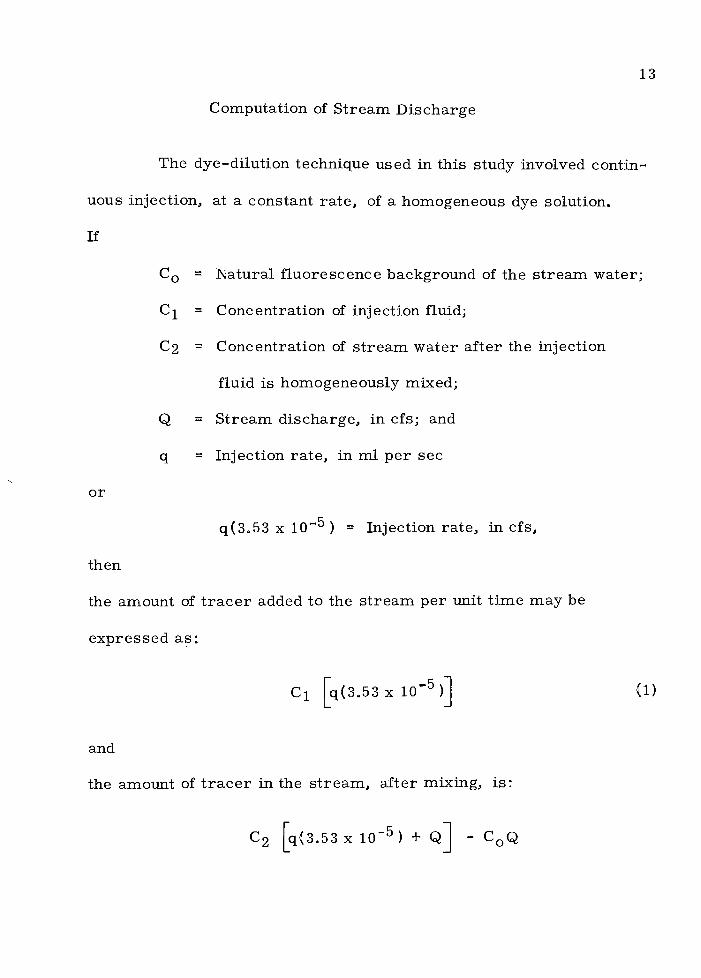
Computation of Stream Discharge

The dye-dilution technique used in this study involved contin-

uous injection, at a constant rate, of a homogeneous dye solution.

If

C0 Natural fluorescence background of the stream water;

C1 = Concentration of injection fluid;

C2 = Concentration of stream water after the injection

fluid is homogeneously mixed;

Q Stream discharge, in cfs; and

q Injection rate, in ml per sec

or

q(353 x 1O) = Injection rate, in ci s,

then

the amount of tracer added to the stream per unit time may be

expressed as:

C1 [q(3.53 x 1O (1)

and

the amount of tracer in the stream, after mixing, is:

C2 [q(3.53 1o) +I1

- C0Q

13

or -

c2 [q(3.53 x 10-5)] + C2Q - C0Q. (2)

Because the theory of the dye-dilution method assumes no

loss or gain of the tracer material, we may equate equations (1) and

(2), thus:

C1 q(3.53 x 1o5)1 = C2 [q(3.53 io5)] + C2Q - C0Q

q(353 1o) (C1 - C2) = Q(C2 - C0)

Q

q(3.53x io) C2 - C0

Q q(3.53 x io) rci - C2[c2_c0 I

or

r C1 C2Q = q(3.53 x io) [c2 - c0 c2 - c0 ]

If we consid.er that the background has been compensated for,

our equation becomes:

C2Q q(3.53 x io [- -]

14

or

or

or

or

Q = q(3.53 x io)

Because the concentration of the stream water is extremely small

compared to the concentration of the Injection solution, we may

simplify equation (3) to:

Q - --- q(3.53 x io).C2

It is interesting to note that the concentrations are expressed as a

ratio. Thus, the units may be either parts per billion or fluorometer

dial readings if all readings are taken on the same range and the

fluorometer is operating properly in a linear manner.

Dye Injection

The rate that dye is injected into the stream must be known.

Dye is injected at a constant rate to facilitate calculations of stream

discharge using the dye-dilution method. All types of constant-rate

discharge apparatusMariotte flask, floating syphon, and constant-

head tankare designed so that the fluid-head of the system remains

constant as the fluid is discharged.

C21

15

16

Mariotte-flask method. - -The constant-rate injection system

used in this study is termed the "Mariotte-flask method" (fig. 1).

The Marlotte flask apparatus is simply designed, constructed,

and compact and does not require a power source, The flask is filled

with a highly concentrated dye solution and is sealed airtight, except

for the air tube. Fluid is discharged from the flask by opening the

orifice at the bottom. As fluid escapes, an area of reduced pressure

is created at the top of the flask, and, as a result, the liquid level

within the air tube begins to fall. Continued discharge further reduces

the pressure in the upper part of the flask, and the liquid level in the

air tube continues to fall until, finally, air bubbles are released from

the bottom of the tube. At this time, atmospheric pressure exists at

the bottom of the tube, regardless of the fluid level, and the flask be-

gins to discharge at a uniform rate and continues to do so until the

liquid level falls below the bottom of the air tube.

It is suggested that the flask be made of rust-resistant mate-

rial to reduce the possibility of rust or scale plugging the orifice. The

flask should be thoroughly flushed and the orifice cleansed after use. A

cockstop-type valve should be used. During transport of a loaded flask

to a higher altitude, the air tube should be plugged at the top or re-

moved from the flask, in order to prevent reduced atmospheric pres-

sure from forcing the injection fluid out of the air tube and spilling out,

Flui

d pr

essu

re a

t thi

s le

vel r

emai

nsth

e sa

me

as a

tmos

pher

ic p

ress

ure

until

flu

id le

vel f

alls

bel

ow th

e en

dof

the

tube

18

Mr. F. A. Kilpatrick of the U. S. Geological Survey, who has

been experimenting with the method at Denver, Colorado, stated (oral

communication), that difficulties are encountered in the operation of a

Mariotte flask designed to deliver at a rate of less than 1 ml per sec.

The reduced pressure in the valve allows the release of air from the

water. These air bubbles slowly build up, and cause a decrease in

orifice area and a decrease in discharge rate. He found that de-aired

water and (or) the addition of a few drops of liquid laboratory detergent

will alleviate the problem.

In order to determine accurately the rate of flow from the

Mariotte flask and to substantiate the fact that the discharge was con-

stant, three experiments were conducted during this study. First, a

card was made in the first few minutes of discharge to check the tra-

jectory angle. The card was cut so that when it was placed along the

upper part of the discharge tube a corner barely touched the discharge

stream. The card was placed in the same positions at different inter-

vals during the discharge period. Toward the end of the test, the cor-

ner of the card still barely intersected the discharge stream. The

second and third experiments were conducted at the same time as the

first. In the second experiment a part of the discharge was caught in

a graduated cylinder during a timed interval. In the third experiment

the amount of discharge collected during this interval was weighed.

19

The variation, as determined by a graduated cylinder, was less than

1 percent: 7.99 to 8.04 ml per sec. The variation, as determined by

weight, also was less than 1 percent: 7.98 to 8.03 ml per sec.

Floating-syphon method, --The floating-syphon method has

about the same advantages as the Mariotte-flask method. The floating

syphon consists of an open container filled with fluid for discharge, a

freely floating platform on the fluid surface, and the syphon tube, which

is attached to the platform and projects to the lower surface of the plat-

form. The tube is an inverted "U, " the height of which must exceed

the depth of the container. The discharge end of the syphon tube must

extend beyond the edge of the container. The hydraulic head is adjusted

by the length to which the discharge end of the tube extends below the

elevation of the intake opening of the tube. Once the syphon is started,

discharge is constant; as the fluid level falls, the floating platform is

lowered, but the relative positions of the tube openings are constant.

Constant-head tank method, --Recent industrial needs for a

constant low-rate discharge apparatus have prompted the development

of a new productthe constant-head tank. The high cost of the appa-

ratus is the main disadvantage. The tank, marketed under the name of

Aerofeed, is a closed container with a pressure cap of air. A highly

sensitive pressure valve adjusts the orifice aperture so that the flow

20

rate is constant as the pressure head of air is depleted. The low

stable-flow rate for the apparatus is about 1 ml per sec.

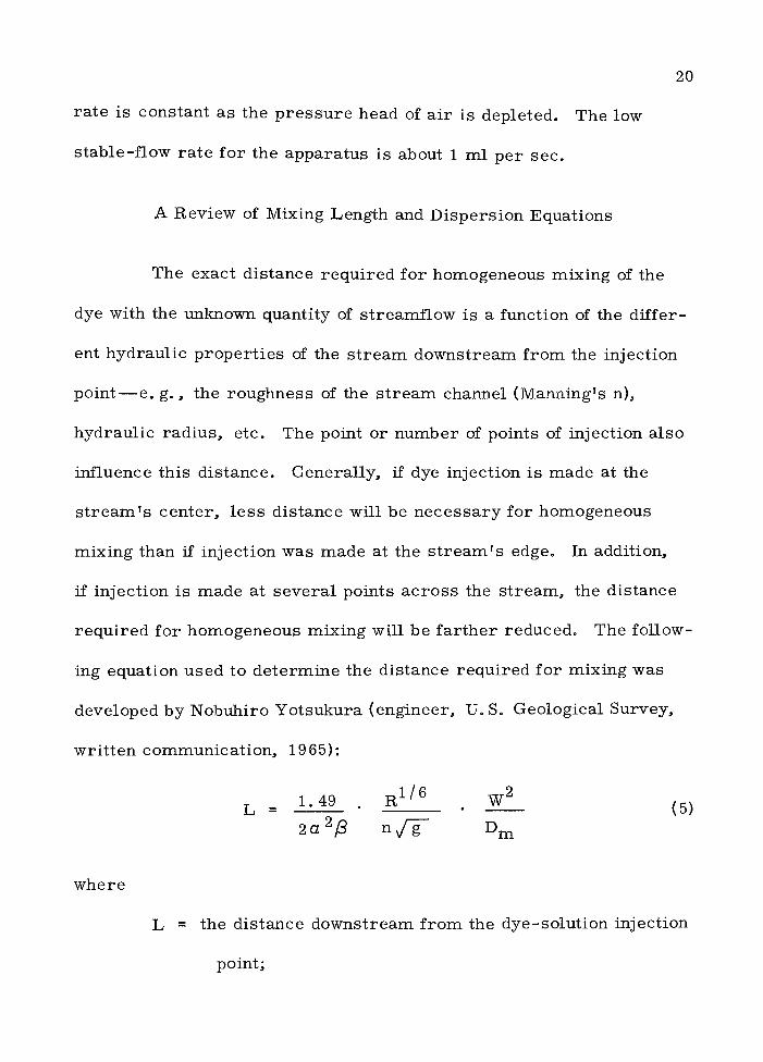
A Review of Mixing Length and Dispersion Equations

The exact distance required for homogeneous mixing of the

dye with the unknown quantity of streamflow is a function of the differ-

ent hydraulic properties of the stream downstream from the injection

pointe. g., the roughness of the stream channel (Manningts ),

hydraulic radius, etc. The point or number of points of injection also

influence this distance. Generally, if dye injection is made at the

streamts center, less distance will be necessary for homogeneous

mixing than if injection was made at the streamts edge, In addition,

if injection is made at several points across the stream, the distance

required for homogeneous mixing will be farther reduced. The follow-

ing equation used to determine the distance required for mixing was

developed by Nobuhiro Yotsukura (engineer, U. S. Geological Survey,

written communication, 1965):

L 1.49 R'6 w2 (5)2a2$ Dm

where

L = the distance downstream from the dye-solution injection

point;

a a constant that is given as 6, for L equal to the point

where the dye first comes in contact with the banks

and as 2 for L equal to the point of complete mixing of

the dye;

/3 = an empirically determined coefficient for which values

have been found ranging from 0.3 to 0.8 in natural

streams but which may have values over a greater

range;

the hydraulic radius of the channel;

the Manning roughness coefficient;

gravitational acceleration;

the mean width of the stream; and

the mean depth of the stream.

The following equations are listed by Andre (1964, p. 28) for

determining the distance necessary for dye to become homogeneously

mixed with streamfiow,

D, E, Hull's equation:

L aQhi3 (6)

where

L = minimum length required for homogeneous mixing;

21

R =

n =

g =

W =

Dm

where

a 50 if injection is performed at stream center, 200 if

performed at stream edge; and

Q = discharge.

Rimmer!s equation:

L = 0.13 k

where

L length required for homogeneous mixing;

b average width of the stream between injection

point and sampling point;

d = average depth; and

k c(0.7C+6)g

where

C = Che'zy coefficient of the given reach with 15 <

C < 50; and

g = acceleration of gravity

Perez1s equation:

b2d

22

(7)

L= 9.5nd (8)

L length required for homogeneous mixing; and

n 0.32 KR1 /6

where

1.486K = coefficient - of Manning's equation;n

and

R hydraulic radius

d average stream depth.

In this study the sampling point was always at a distance of

more than 50 channel widths, this distance being about 10 times the

computed value from any of the above equations.

Dye Samples Collected

Water samples were taken downstream from the point of homo-

geneous vertical and lateral mixing of the dye-injection solution. A

small quantity of streamflow was collected in clear pharmaceutical

dispensary vials of 5-dram capacity, which provided enough liquid to

allow two separate tests on the fluorometer. The samples then were

placed in a closed box to deter any fluorescence loss from the dye due

to exposure to sunlight. Each sample taken on the plateau of the dye

cloud allows computation of the instantaneous stream discharge.

23

Fluorometer Operating Procedure

The G. K, Turner Model III fluorometer was used in this study.

This electronic instrument operates on the principle of an optical

bridge, which is analogous to the familiar Wheatstone bridge used in

measuring electrical resistance, The optical bridge compares the

difference in light intensity emitted from the sample and light intensity

from a calibrated rear path (fig. 2). Comparison of the light inten-

sities is made by a single photomultiplier, which alternately receives

light from each path. The rotating light interrupter allows only light

from one path to intercept the photomultiplier at any one time. A

single mercury light source is used for each path of light. For the

most part, the reliability of the instrument is due to the single light

source and single photomultiplier, because any aging of the bulb, etc.,

will not affect the readingall light beams are affected to the same

extent, Differences in light intensity from the two paths cause the

photomultiplier to rotate electrically the light cam and diffuse screen,

The rotation of the light cam continues until the light intensity of both

paths is equal, at which time the movement of the cam virtually ceases.

The fluorescence dial is read at this time, The range selector is an

operator-adjusted curtain that has four openings of different sizes.

Light from the source is allowed to pass through one of the openings

as it is radiated toward the sample. Samples containing high

24

WY

rOR

PHO

TO

MU

LT

IPL

jER

LIG

HT

IN

TE

RR

UPT

ER

MO

UN

TIN

G B

LO

CK

LU

CIT

E L

IGH

TPI

PES

FIL

TE

RSA

MPL

EP

asse

s no

u.v

.

BL

AN

K K

NO

B

FIL

TE

RC

OO

LIN

G F

AN

Pas

ses

only

u,v

.

FLU

OR

ESC

EN

CE

DIA

L

UL

TR

AV

IOL

ET

SOU

RC

E

RA

NG

E S

EL

EC

TO

RFo

urap

ertu

res

DIF

FUSE

SCR

EE

NLIG

HT

CA

M

Figu

re 2

. --D

iagr

am o

f th

e T

urne

r M

odel

III

f'lu

orom

eter

opt

ical

sys

tem

.(F

rom

G. K

. Tur

ner

Ass

ocia

tes,

196

4.)

26

concentrations of fluorescein dye require the use of the smaller open-

ing so that the fluorescence dial will not run off scale on the upper

magnitude.

The fluorometer has two locations for optical filters. Both

of these are on the forward light path, the first just before the sample

and the second immediately after the sample. The filters allow light

of only a very restrictive wavelength to pass. The first set of filters

passes light that closely coincides to the peak absorption wavelength

of the sample compound, and the second set passes light of the wave-

length that the sample emits when excited by the light that passes the

first filter. The two filter locations are at right angles to each other,

so that if filter transmission is somewhat overlapping, only fluorescent

light will reach the photomultiplier, The instrument was used without

a special high-sensitivity green bulb or a high-sensitivity door, which

increase the fluorometer sensitivity by 10-20 fold.

Although the instructions distributed with the fluorometer

state that a warmup period of 15 minutes is sufficient for operation,

repeated unsuccessful attempts to reproduce dial readings and (or)

calibrate the fluorometer showed that a warmup period of several

hours was necessary. A minimum warmup period of 6 hours was

used for this study.

27

Room temperature was thermostatically controlled at all

times. Before examination of the sample, the vials were placed in

the fluorometer room for a period of not less than 8 hours, which

allowed for temperature stabilization. The sample was transferred

from the vial to a temperature-stabilized cuvette. The cuvette was

placed 2 or 3 feet from the fluorometer to prevent it from gaining

heat from the fluorometer.

About the same length of time was taken to run each sample.

Cuvettes were alternated as quickly as possible without carelessness.

The fluorometer door was opened only when necessary in order to

maintain a constant temperature within the chamber.

The main consideration when reading the fluorometer dial

should be consistency of method. Whatever method is adopted by the

operator for reading unknown samples must be adhered to when the

fluorometer is calibrated. After the instrument is warm, it must be

checked and possibly adjusted to assure that a reading of zero is shown

when a blank or dummy cuvette is tested. The dial wavers slightly

during operation, which is due to the servomotor movement, as it

constantly seeks to establish the balance of the optical bridge system

of the fluorometer. The dial movement is in the magnitude of + 0.25

unit and occurs every half second to a second. A gradual decrease in

magnitude of fluorescence occurs owing to the gradual increase in

28

temperature of the sample. The temperature of the chamber where

the cuvette is placed is higher than the room temperature. The tem-

perature of the chamber is higher because it is located close to the

electronic circuitry of the fluorometer. The temperature of the sam-

ple also increases because the sample is subjected to intense light.

The temperature increase causes a decrease in the fluorescence of the

sample with time. The temperature increase occurs in 15 to 25 sec-

onds, and the fluorometer readings may drop 1 to 2 units during this

time.

A complicated chemical breakdown of the dye occurs when it

is subjected to ultraviolet lighteither sunlight or the light from the

fluorometer. However, this process is accelerated greatly when the

dye is in the fluorometer, due to the intensity of the light. Labora-

tory experience has shown that if samples are allowed to remain in

the fluorometer for less than 1 minute and allowed 30-60 minutes for

restabiization to room temperature, the first reading usually could be

repeated. Third attempts, however, usually resulted in lower read-

ings. Alter considering the above physical variations and operating

characteristics of the instrument, the procedure for testing a sample

with the fluorometer is:

(1) A cuvette containing only distilled water (a blank sample)

is placed in the fluorometer and the dial is set at zero.

29

A dye sample is placed in the fluorometer.

The dial is read 20 seconds after the fluorometer door

is closed. The time interval is sufficient to allow full

dial movement from zero to any reading. This technique

subjects all samples to the higher temperature of the

instrument for the same length of time; therefore, the

temperature of all samples is the same at the time of

dial reading.

The blank cuvette is placed in the fluorometer after the

dial reading for the sample, which returns the fluorom-

eter dial to the proximity of zero. Recent information

from a G. K. Turner representative indicates that this

step can be eliminated in future tests.

A cuvette is the small test tube that contains the solution to be

tested in the fluorometer. To insure accurate fluorescent testing of

the dye solution by the fluorometer, each cuvette was thoroughly

cleansed and dried before it was filled with the solution to be tested.

Elaborate washing of the cuvettes between tests is unnecessary, and

thorough flushing with distilled water is adequate. After washing the

cuvettes were placed in the cuvette stand in an inverted position to

facilitate draining; the cuvettes were then transferred to the fluorom-

eter laboratory where they were stored in a closed cupboard to retard

30

collection of dust. A period of not less than 8 hours was allowed to

elapse before the cuvettes were used, which allowed adequate time for

drying and temperature stabilization. Cuvettes were handled only at

their extremities to prevent the possible fluorescence of fingerprints

from yielding an erroneous reading. The center of the cuvette is

where the ultraviolet light from the fluorometer penetrates to deter-

mine the fluorescence of the solution being tested.

Laboratory Experiments

Matching of Cuvettes

The instructions for the operation of the fluorometer state

that the instrument is designed in such a way that any variance in the

optical properties of the cuvettes will not be shown in the readings. In

order to substantiate this, two tests were made. In this study, 46 new

cuvettes were used. Each cuvette was marked with an identifying num-

ber directly below the cuvette lip, well above the part of the cuvette

through which light passes.

In the first test, a weak dye solution was mixed at an arbi-

trary strength. The solution was stirred with a magneticstirrer for

15 minutes to assure homogeneity of the solution and was placed in a

cupboard in the laboratory for 12 hours to allow temperature stabili-

zation. After a 12-hour warmup period of the fluorometer, the

31

cuvettes were filled with the dye solution and tested. A listing of the

fluorometer readings that corresponded to the appropriate cuvette was

made. All readings were obtained on range 30. Of the 46 cuvettes

tested, 42 produced readings of 22.5 units, and the remaining 4 pro-

duced readings of 23.0 units,

The second test utilized a strong dye solution, and the same

procedure was used as in test one. The readings in test two were

obtained on range 1, and the results are tabulated below:

The four cuvettes that produced the higher readings in the first test

gave readings of 97. 0, 97. 5, 98. 0, and 98. in the second test. The

higher readings obtained in the first test are attributed to an inherent

play of ± 0.25 unit in the fluorometer dial. The greater variation in

readings in the second test, however, is not completely understood,

but it may be due to the increasing interference of one dye particle with

another as concentration increased.

Number of cuvettesFluorometer reading

(units)

2 96.02 96.58 97.05 97,56 98.0

16 98,55 99.02 99.5

32

The results of the two tests show that no calibration of individ-

ual cuvettes is necessary. The tests indicate that the errors for

individual cuvettes are not systematic and that calibration of cuvettes

would make no significant improvement on precision of final results.

Fluorescence Loss Due to Direct Sunlight

Adsorption of dye by apparatus and photochemical changes in

dye on exposure to direct sunlight have been reported by many workers,

Each of these factors causes a loss of dye from the system and results

in error of the dye-dilution method, because the theory of the method

assumes no loss or gain of dye during the procedure. The error would

result in overcalculation of the true rate of streamflow. The most

recent developments in fluorescent dyes are "Brilliant Pontacyl Pink

B" and "Rhodamine WT Extra," which are manufactured by the

General Analine and Film Corp. The manufacturer reports that the

dyes have qualities superior to those of previous productsi. e., less

adsorption on solids and greater photochemical stability. These prop-

erties were examined in two experiments using Brilliant Pontacyl

Pink B.

The purpose of the first experiment was (1) to determine if

dye adsorption would occur in measureable amounts on the plastic

33

pharmaceutical dispensary vials used for dye sampling purposes, and

(2) to examine the extent of photochemical change.

The dye solution was freshly prepared and magnetically

stirred for 15 minutes in a glass beaker to assure homogeneity. Dye

concentration was arbitrarily chosen but was within the detectable

range of the fluorometer. Each of the 12 new vials was flushed with

distilled water, dried, and filled with solution, Four of the vials were

placed in a cupboard, and the 8 remaining vials were placed outdoors

on the night of June 9, 1965. The 8 vials were exposed to the sun for

different periods of time ranging from 1 to 4-1/2 days (fig. 3). The

vials that were exposed for less than 4-1/2 days were placed in the

cupboard until the end of the test, Fluorometric testing of the solution

was conducted in two periods after the first day, 2 of the 4 vials in

the cupboard were analyzed, and at the end of the 4-1/2 days, the re-

maining vials were analyzed. The conclusions from the first experi-

ment are: (1) within the range of the experiment, the decay of fluo-

rescence of the dye on exposure to direct sunlight is a linear function

of time, (2) the decay of the dye that remained inside the cupboard

was negligible, and (3) the amount of dye adsorption onto the plastic

vials was negligible.

In 1967January 9-14 and January 16-20a second experi-

ment was conducted to examine the photochemical decay properties of

40

30

20

Figure 3. - - Variation of fluorescence with exposure to sunlight.

34

0 1 2 3

Time, in days

June 9-15, 1965.

35

Brilliant Pontacyl Pink B. The second experiment was similar to the

first, except that four standard solutions of differing concentrations-313 ppb, 156.25 ppb, 62.6 ppb, and 6.26 ppbwere used. An attempt

also was made to measure the total solar energy absorbed by each

sample. Vials were filled with each of the four standard solutions

(26 vials of each); a total of 104 vials was used. Four vials of each

concentration were stored in the laboratory cupboard in nearly total

darkness to calibrate the fluorometer, It is assumed that solutions

are stable under these conditions.

The remaining vials were placed in direct sunlight from 0930

to 1530 hours during different days of the test. The cumulative expo-

sure to sunlight was converted to langleys (cal per cm2) by consulting

records of radiation intensity at the University of Arizona Department

of Atmospheric Physics. Figure 4 shows the relation between change

in fluorescence and total exposure. It should be noted, however, that

the langleys given were measured by a pyrheliometer; therefore, they

provide a measure of solar energy absorbed by the samples. The

actual energy absorbed by the samples would have to be multiplied

by a factor (factor unknown) to account for reflection and absorption

of energy by the plastic containers, Unfortunately, the value of

this factor is not known. All samples were tested at the same time,

after proper fluorometer warmup and temperature stabilization.

$4 a

0

1000

Dye

con

cent

ratio

n, in

par

ts p

er b

illio

n

IiI

II

1-I

VII

I

I1

II

II

II

Figu

re 4

. - -

Dec

ay o

f B

rilli

ant P

onta

cyl P

ink

B o

n ex

posu

re to

dir

ect s

unlig

ht.

C.)

2000

e

3000

II

1010

0

37

The apparent loss of dye due to photochemical decay may be observed

from the fluorometer calibration curve constructed from the standard

solutions that remained in the cupboard. All lines on figure 4 are

parallel; 313 ppb concentration is somewhat uncertain, however, In

each case 50 percent of the original fluorescence was lost after a

cumulative exposure of about 2,300 langleys, as recorded by the

pyrheliometer.

Since there are about 500 langleys per 6 hours of direct noon-

day sunlight on a bright January day, we have an apparent half life of

fluorescence equal to about 27 hours. By analogy with radioactive

decay, we may use the equation

F FQet, (9)

where

F = Final concentration;

= Initial concentration;

e = A mathematical constant;.

x 0.693T

where

T = Time of half life; and

t = Time during which decay occurred.

38

Assuming that 6 hours is the maximum amount of direct sun-

light possible in any given test and that the original concentration was

100 ppb, we obtain

_(o. 693"( 6

F = 100 e 27 J\

-. 154= 100 e

100- .154

e

100- 1.1666

- 95. 76,

which indicates that the maximum percentage of decay for any test is

about 14 percent.

Field Experiments

Four field tests were conducted during this studyWillow

Creek test, Sabino Creek test, Paria River test, and Chinle Wash test.

Sampling of streamfiow for analysis of fluorescent dye was conducted

at 2-1/2 minute intervals. The samples were collected in 5-dram

clear plastic pharmaceutical dispensary vials. In samples that con-

tained sediment, the vials were allowed to stand until the sediment

settled to the bottom; only the clear supernate was fluorometrically

tested. Brilliant Pontacyl Pink B tracer was injected using a

39

30-gallon Mariotte flask. A small amount of tracer fluid was collected

from the flask at the beginning and end of the injection period for test-

ing in the fluorometer to determine if the dye was of equal concentration

during the entire test. The fluorometer showed each injection solution

to be homogeneous. Current-meter measurements were conducted

using the specifications of Corbett and others (1943). The measure-

ments are on file in offices of the U. S. Geological Survey, Water Re-

sources Division, Tucson. The fluorometer readings for all samples

and the background fluorescence of each test are given in the appendices.

Sampling for background fluorescence was conducted several feet up-

stream from the injection point at the beginning and end of the injection

period. The background fluorescence was constant during each test.

Sediment samples were collected using the equipment and methods out-

lined by the U.S. Inter-Agency Committee on Water Resources (1965)

and were analyzed by the Water Resources Division of the U. S. Geo-

logical Survey, Tucson. A composite sample was analyzed, and a

sieve analysis was conducted to determine sediment size.

Willow Creek Test

Willow Creek is on the Apache Indian Reservation in Graham

County. A preliminary test was conducted on the creek under uniform

flow conditions on September 5, 1965. At the time of the test, the

40

discharge of the creek was due to pumpingpumpage records indicate

that a discharge of 9,200 gpm (20.49 cfs) was maintained throughout

the day (fig. 5).

The reach used during the test extends downstream from the

pipe outlet for 2.2 miles. Injection took place 50 feet below the pipe

outlet (fig. 5A). The tracer was injected at a rate of 13.17 ml per sec

for 67 minutes. A 45-minute lapse in injection allowed the streaniflow

to return to normal fluorescence, The second injection period lasted

for 17 minutes, and fluid was injected at a rate of 51,29 ml per sec.

Observers took samples simultaneously 0,3, 1,2, and 2.2

miles downstream from the injection point. Several hundred small

wooden blocks were dropped into Willow Creek 15 minutes before the

first injection to serve as markers for the observers, Observers

counted from the time the blocks were sighted until the sixth 2-1/2

minute interval thereafter, when they filled four vials at equidistant

increments across the stream. This procedure was repeated at the

twelfth 2-1/2 minute interval, when five vials were filled at equidistant

increments. The regular samples were taken throughout this period.

The cross-channel sampling was done to check each station for validity

of representative samples. The cross-channel sampling also served

as a check for homogeneity of dye mixture throughout the stream width

at that point.

FIGURE 5

FLOW IN WILLOW CREEK

A.

Willow Creek diversion from Black River gaging station.

Mariotte flask in place and discharging.

B.

Flume used for discharge measurement, Flow from right to

left.

42

The recorder chart from the U, S. Geological Survey gaging

station at the pipe outlet is shown in figure 6, The slight variation in

stage indicates essentially constant discharge, A current-meter

measurement was made during the first injection period, and showed

a discharge of 20.03 cfs, The sediment concentrations of Willow Creek

was extremely low during the test, and the flow appeared crystal-

clear. Results of the dye-dilution test are shown in Appendix A, For

the first injection period, a discharge of 20.24 cfs was calculated from

the plateau of the uppermost sampling site,

The fluorometer dial readings versus time for each site were

plotted. The areas under the respective curves were determined and

are as follows:

Parts per billionSite Dial-minutes fluorescence-

minutes

The percent variation of the extremes (Sites 1 and 2) varies

by only 0.26 percent. Therefore, the loss of dye by adsorption was

very slight during this experiment; any loss would have been reflected

in a decrease in area under the curve for each site downstream,

1 2,453,25 921, 69

2 2,447,00 919, 34

3 2, 447. 56 919. 55

0z2.8 _ 11111111111111 I liii

.4) -

II

I I

2.6 I

I

I

2.4lIIIIIIfIIIIIIIIIIIITime, in hours

September 5, 1985

Figure 6. --Recorder chart from Willow Creekdiversion of Black River gaging station.

43

"-44) I- I

0) -- I

44

Inasmuch as the discharge of Willow Creek was constant,

analysis of the test is possible by the total-recovery method. This

method is used where a "slug" of dye is injected into the stream, and

the dye cloud is monitored downstream. The theory of the method

does not require that the dye be injected instantaneously. The follow-

ing equation is applicable:

VTC1Q (10)

(C-C)dt

where

VT = The volume of dye solution injected into the

stream;

C1 = The concentration of injection solution;

C2 The concentration of streamfiow (variable)

after the injection fluid is homogeneously

mixed across the stream section;

C0 The natural fluorescence background of the

streamfiow; and

f(C2 -00)dt The total area under the concentration-time

curve.

Applying equation (10) to data from the upper site, the first

part of the Willow Creek test, where the injection rate using the

Mariotte flask was 13.17 ml per sec:

where

45

VR 13.17 ml per sec

VR = Volume-rate of injection,

so

VR = 0.013171 per sec,

or VR = (0. 01317)(0. 03531)

= 0.00046503 cfs

Injection was continued for 67 minutes (4, 020 seconds).

VT (0. 000465031)(4020)

= 1. 86943 ft3

The concentration of the injection fluid was determined to be

335, 140 ppb.

Thus:

VTC1 = (1. 86943)(335, 140)

= 626,521.26 ppb ft3

The fluorometer readings from time 1115 to 1315 were plotted

and a smooth curve was passed through the points. (See Appendix A.)

From this curve, fluorometer readings were selected at 1. 25-minute

increments. Using the fluorometer calibration curve, each fluorome-

ter reading was converted to parts per billion. Thus, by the histogram

method, the area under the curve is 29, 700 ppb sec. Using this

figure and substituting equation (11) into equation (10), we obtain:

Measuring method

626,52129,700

Q 21.09 cfs

The larger discharge indicated by the total-recovery method

may be due to a slight inaccuracy in determining the area under the

concentration-time curve or to the possible loss by sorption of dye on

the leading front of the initial dye cloud.

Results of the Willow Creek test are as follows:

46

Variation from VariationDischarge current-meter from dye-

(cfs) measurement dilution test(percent) (percent)

Sabino Creek Test

Sabino Creek is in the Coronado National Forest, Pima

County, A test was made on the creek under nonuniform flow condi-

tions on November 25, 1965.

The reach used extends 0.85 mile downstream from the lower

stream crossing on upper Sabino Canyon Drive. The lower end of the

Pumping station 20,49 +2.3 +2,2

Current meter 20.03 0.0 -1.0

Dye dilution 20.24 +1.1 0.0

Total recovery 21.09 +5,3 +4.0

47

reach is marked by a Survey gaging station cableway located about 300

feet downstream from the gaging station. Injection was made at the

crossing at a rate of 13.17 ml per sec. Samples were taken beneath

the cableway.

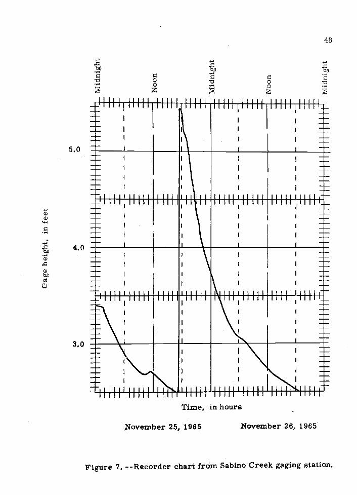
The recorder chart from the gaging station is shown in

figure 7.

Three current-meter measurements were made during the

test under the cableway (fig. 8):

Mean time of the Computed dischargemeasurement (cfs)

The sediment concentration was very low, and the flow was

clear and clean on visual inspection. Results of the dye-dilution test

are shown in Appendix B. The discharge determined by the second

current-meter measurement was 148 cfs compared with a discharge

of 141 cfs by the dye-dilution method. Discharge by the dye-dilution

method was 4.7 percent below that given by the current-meter

measurement (table 1).

2110 2202320 1480040 118

5.0

4.0

30

1+11 1{III II I IIIII III

Time, in hours

November 25, 1965 November 26, 1965

Figure 7. --Recorder chart from Sabino Creek gaging station.

FIGURE 8

FLOW IN SABINO CREEK

A.

Dye injection site for Sabino Creek test.

B.

Dye sampling and current-meter-measurement site for Sabino

Creek test.

TA

BL

E 1

DIS

CH

AR

GE

CO

MPU

TA

TIO

NS

FOR

SA

BIN

O C

RE

EK

BA

SED

ON

U. S

. GE

OL

OG

ICA

L S

UR

VE

Y G

AG

ING

-ST

AT

ION

RE

CO

RD

AN

D D

YE

-DIL

UT

ION

ME

ASU

RE

ME

NT

Tim

e(h

ours

)

GA

GIN

G S

TA

TIO

ND

YE

-D

ILU

TIO

NM

ET

HO

D

Dif

fere

nce

betw

een

dye-

dilu

tion

met

hod

and

gagi

ng-s

tatio

nre

cord

(per

cent

)

Gag

ehe

ight

(fee

t)

Shif

tad

just

men

t(f

eet)

Adj

uste

dga

gehe

ight

(fee

t)

Dis

char

ge(c

fs)

Dis

char

ge(c

fs)

2245

3. 7

7-0

. 38

3. 3

616

314

8-1

0. 1

2300

3. 7

2-0

. 38

3. 3

415

914

5-

9, 7

2315

3.68

-0. 3

83.

3015

314

2-

7. 7

2330

3.64

-0.3

83.

2614

714

0-

4.8

2345

3. 6

0-0

. 38

3. 2

314

113

8-

2. 1

2400

3.57

-0.3

83.

1913

713

70.

0

Paria River Test

The Paria River is in Coconino County. A test was conducted

on the river on April 3, 1966, to determine the validity of the dye-

dilution method in sediment-laden streams.

The reach used during the test was the 1.5 miles above the

junction of the Paria and Colorado Rivers. Injection took place at the

upper end of the reach. The tracer was injected at a rate of 4.22 ml

per sec for 2 hours and 20 minutes (fig. 9).

Observers took samples 0.4 and 1.2 miles downstream from

the injection site. The recorder chart from the U. S. Geological Survey

gaging station 0.2 mile downstream from the injection site is shown in

figure 10.

At the lower site, the data obtained by the dye-dilution test

were erroneous, because the station was too close to the Colorado

River. The Colorado River flow increased during the test, and the

observer reported an increase in stage of the Paria at the sampling

site. The evidence suggests that backwater conditions from the

Colorado River affected the data obtained from the lower sampling site.

In the Paria River test, an unusual degree of scatter of the

data is evident, which is probably due to slight contamination of the

samples after an accident with the Mariotte flask in transport. Fluid

spilled from the tank restilted in the staining of the cardboard

51

FIGURE 9

DYE INJECTION AT THE UPPER ENDOF THE PARLA RIVER TEST REACH

52

.4-.

0

7.0 1111111111 III I III F

.-4

'I

6.0"-4ci)

4) -bti --

5.0 -111111; I I 11111111 11111

Time, in hoursApril 3, 1966

Figure 10. --Recorder chart from Paria River gaging station.

53

54

containers in which the new and unused sampling vials were stored.

Special care, however, was exercised by the sampling personnel to

avoid vial contamination, Results of the test data show a slight random

distribution which may be due to (1) sample contamination due to the

accident, (2) the sediment load of the stream, and (3) variation of

background due to differences in sediment in the vials at the time of

fluorometer analysis.

Two current-meter measurements were made in order to

compare the amount of discharge given by the current meter with the

amount given by the dye-dilution method. The first current-meter

measurement was made at the point of dye injection (8,79 cfs) and the

second was made at the upper sampling site (7,85 cfs). It was neces-

sary to extend the dye-dilution data to the time of the current-meter

measurement. The data were extended by drawing a straight line

through the mean of the data points, which represent instantaneous

stream fluorescence. The time interval for the points used was from

1205 to 1330 hours. Three sediment samples were taken 50 feet up-

stream from the injection site. The sediment load was 1,470 ppm by

weight; 99.8 percent of the sediment was finer than 0,053 mm, The

results of the dye-dilution test are shown in Appendix C and are com-

pared with the current-meter measurement below:

Measuring methodDis charge

(cfs)

Chinle Wash Test

Chinle Wash is in Apache County, A second test on sediment-

laden streams was conducted on April 10, 1966.

The reach used during the test extends 1.2 miles downstream

from the bridge on Arizona Highway 64. Injection took place beneath

the bridge at a rate of 4.22 nil per sec for 4 hours,

The observer took samples 1.2 miles downstream from the

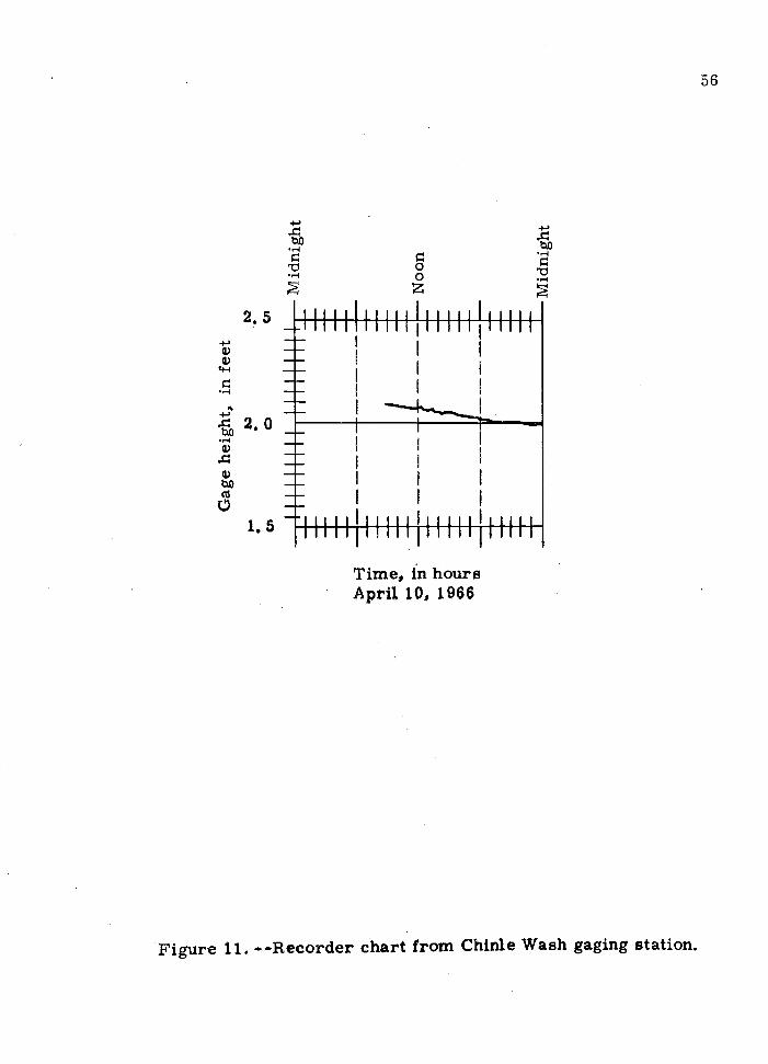
bridge. The recorder chart from the U. S. Geological Survey gaging

station 100 feet upstream from the bridge is shown in figure 11, and

the results of the dye-dilution test are given in Appendix D.

A current-meter measurement was made 160 feet upstream

from the bridge and showed a discharge of 2.68 cfs. The sediment

load was 3,720 ppm by weight, and 99.9 percent of the sediment was

finer than 0.053 mm.

A direct comparison of discharge computed from the current-

meter measurement with discharge computed from the dye-dilution

Current meter 7,85 0. 0

Dye dilution 8,71 +11,0

55

Variation fromcurrent -metermeasurement

(percent)

I

Figure 11. '-Recorder chart from Chinle Wash gaging station.

56

2. 5 liii 11111111111 III

1. 5I 11111 11111111111 I liii

Time, in hoursApril 10, 1966

57

method is not possible. The current-meter measurement was conduct-

ed at the injection point rather than at the sampling site, Therefore,

a direct comparison of the two means of stream measurement would

require a time adjustment of the mean time of the current-meter

measurement so that it would apply to the same stream discharge at

the sampling site. The fact that the mean time of the current-meter

measurement was 55 minutes after the start of injection is of no help,

because the sampling site was chosen arbitrarily and has no rating

relation with the gaging station, and the staff or river stage was not

recorded at the sampling site,

This test shows the Importance of taking samples and current-

meter measurements at the same location. If the purpose of a dye-

dilution test is the rating of a gaging station, the sampling site must be

close to the gaging station.

Because the scatter of data points was small in spite of the

high suspended-sediment concentration during the Chinle Wash test, it

seems likely that the scatter in the Paria River test was due to causes

other than suspended-sediment concentration,

Discharge as determined by the dye-dilution method ranged

from 2. 40 to 4. 00 cfs.

DISCUSSION AND SUMMARY

Possible Sources of Error

If systematic errors are disregarded, the mean of errors in

current-meter measurements is random and is normally distributed

(Carter and Anderson, 1963, p. 106). The same is assumed true for

fluorometer operation, but not for the dye-injection method as a whole.

Dye adsorption onto organic or inorganic substances and fluorescence

breakdown of the dye with exposure to light reduce the magnitude of

fluorescence recovered in the sampling procedure. The loss results

in departure from the theory used in the dye-injection method, Be-

cause the degree of fluorescence is inversely proportional to discharge,

the mean of the errors involved in the dye-dilution method will result

in some plus valuei. e., the dye-dilution method will tend to over-

estimate the true or exact discharge.

This study indicates that collectively the errors are very

minor. Although no sediment was present in the flow of Willow Creek,

the homogeneous dye solution was in contact with the stream channel

for 2,2 miles. Several varieties of grass in large stands occur in and

along the channel. Willow Creek is at an altitude of 5,975 feet, where

58

59

there was direct noonday sunlight during the early hours of the test.

At this altitude, the sunlight should contain considerable ultraviolet

rays, Although the rays may be responsible for fluorescence decay of

the dye the Willow Creek test showed no measureable adsorption or

fluorescent decay. Therefore, for practical purposes the plus mean

error for dye-dilution tests is negligible.

It is suspected that different organic and inorganic substances

will exhibit slightly different affinities for dye adsorption and absorp-

tion. Conducting the dye-injection test at night eliminates the fluores-

cence-decay factor; however, floods occur anytime, and the user of

automated dye-injection tests must consider this possibility.

Dye manufacturers are engaged in research to develop dyes

that will reduce the properties of sorption and light decay present in

current products.

The deviation between computed discharge by the current-

meter method and computed discharge by the dye-dilution method does

not always indicate error in the latter method, Computation of dis-

charge using the Price current meter utilizes the following equation:

Q VA (12)

where

Q = discharge, in cubic feet per second;

60

V = velocity, in feet per second; and

A area, in square feet.

Equation (12) allows the computation of the rate of discharge

of water in clear streams. Suspended sediment in a stream will occupy

a certain percent of the stream area, and the computed value of Q will

no longer represent the flow of water alone. Normally, this factor is

ignored, because of the extremely low-sediment concentrations in most

streams, Even sediment loads that are termed "heavy" normally do

not consist of concentrations large enough to cause an error of a mag-

nitude that would equal the error of a current-meter measurement. In

the Southwest, however, sediment loads at high stage rival World rec-

ords for suspended-sediment concentrations. In some northern

Arizona streams, as much as 20 percent of the volume of streamfiow

is occupied by sediment (600,000 ppm by weight). Therefore, this

factor should be considered when comparing current-meter measure-

ments and dye-dilution measurements made on streams with high

suspended-sediment concentrations.

Future Uses

The greatest potential afforded by the dye-dilution method of

computing flow is in the rating of different types of surface-water

stations. In this regard, the dye-dilution method may be utilized in

61

conjunction with slope-area measurements; where difficulty in acquir-

ing slope-area measurements is encountered, it alone may be used.

Where dye injection and sampling are continuous for the

duration of flow, the dye-dilution method offers a direct method for

determining total discharge. This approach offers great promise for

flashflood studies in the Southwest, where station ratings have not

been established. The dye-dilution method especially lends itself to

studies involving a water budget.

Continuous injection and sampling will allow a hysteresis

analysis of flood hydrographs and will provide both the rating for peak

discharge and the total discharge. Storm hydrographs typically show

very steep rising limbs and more extended recession limbs. Most

current-meter measurements are made at peak discharge or on the

recession limb of the hydrograph. In many instances, this is due to

the lack of flood warnings, which prevent personnel from being at the

site and ready to take measurements when flow begins. However,

rising stages typically carry huge quantities of debris, which make

current-meter measurement difficult or impossible. As a result, few

current-meter measurements exist for the rising limb of hydrographs.

Even if a current-meter measurement is obtained on the rising limb

of a hydrograph, another problem is encountered in the computation

of the measurement, The very rapid change in river stage during

measurement requires that the computed gage height be weighted.

62

This weighting reduces the accuracy of the gage-height value assigned

to the measurement. Therefore, the evaluation of the hysteresis ef-

fect of rating curves for different stations is impossible or produces

questionable results, The dye-dilution method, however, may allow

this evaluation,

Before using the dye-dilution method for evaluation of the

hysteresis effect, however, the following factors must be considered.

During the rising limb of the hydrograph, water enters the streambank

and forms bank storage. If a dye-dilution measurement is in progress,

the dye concentration in this water will be dependent on the rate of

discharge. As discharge increases, dye concentration decreases, at

the same time that more water is lost to bank storage. Thus the dye

concentration of the water in bank storage will vary. As discharge

decreases, water will be released from bank storage but at a different

rate than that at which it entered; also, the total volume of water re-

leased will be less than the volume stored. The dye concentration in

the water released from bank storage will be of a different magnitude

than that of the river water, The above factors would complicate any

analysis. Fortunately, in most cases these effects may be neglected

without significantly affecting the accuracy of the discharge calculation.

Future Developments

U.S. Geological Survey personnel are, at the present time,

involved in studies to determine the applicability of the dye-dilution

method in measuring streamflow under different conditions and in

different localities, The Survey is developing apparatus designed to

inject and sample automatically when triggered by streamfiow. Major

factors in the consideration of automatic apparatus are the initial

expense, simplicity of operation, and physical size. The withdrawal

of a discrete dye sample at short time intervals will be necessary.

In streams in the Southwest, sampling must begin at or near zero flow

and continue for the duration of flow. The method will provide data

for rating the station at all river stages during the test, and total

discharge also may be computed.

Conclusion

63

The feasibility of conducting discharge measurements by the

dye-dilution method has been examined by laboratory and field experi-

ments. The direct comparison of discharge computed from the current-

meter measurement and computed from the dye-dilution method was

possible in three field tests. The maximum deviation between the two

methods was 11 percent. This percentage contains possible errors in

the current-meter measurement and the dye-dilution method. The

64

figure corresponds favorably with the computed discharge from gaging

stations on sand-channel streams, For a slope-area measurement,

15 percent accuracy is considered near optimum. Therefore, the

conclusion is made that computation of streamfiow by the dye-dilution

method holds promise for gaging streams in the Southwest. Such

measurements fall well within the acceptable limits of accuracy.

APPENDIX AWILLOW CREEK TEST

Fluorometer calibration: 34 ppb = 90.5 on fluorometer dial.

Injection solution = 335,140 ppb.

Injection rate = 13.17 ml per sec.

Discharge obtained by current-meter measurements is listed as CMM.

A background of 1,0 dial units has been removed from the following data.

FluorometerTime reading Discharge

(hours) (dial units) (cfs)

(Upper station)

1130 2.56. 0

13. 517.019.0 20.03 CMM

5

1145 19. 520.020. 520. 0 20. 2420. 5 20. 2420. 5 20. 24

65

1115 0. 00. 50.00. 00.02. 5

FluorometerTime reading

(hours) (dial units)

1200

1215

1230

1245

1300

1315

20. 520. 520. 520. 520. 520. 5

20. 520. 520. 520. 520. 020. 0

20. 520. 517. 5

8. 54. 52.0

1.51.00. 50. 50. 50. 5

0. 50. 50. 00. 50.00. 5

0. 00. 00. 00. 5

26. 053. 5

Discharge(cfs)

20. 2420. 2420.2420.2420. 2420.24

20. 2420. 2420, 2420. 24

66

FluorometerTime reading Discharge

(hours) (dial units) (cfs)

1330 66.55

5

67. 553. 526. 5

1200

1215

1230

(Middle station)

0. 00. 00. 00. 00. 00. 5

1. 505

8. 010. 512. 5

5

5

5

17.018. 018. 5

67

1345 13.57. 05. 03. 01.51.0

1400 0. 50. 00. 00. 0

FluorometerTime reading Discharge

(hours) (dial units) (cfs)

1245

1300

1315

1330

1345

1400

18. 519. 019.019.019. 019. 5

19.519. 519.519. 519. 519. 5

20. 019. 519. 016. 513. 511.0

8. 56. 55. 54. 53. 5

0

2. 52. 01.51.51.01.0

0. 50. 51.5

5

8. 522. 5

21.28

21. 2821. 2821.2821. 2821.2821. 28

21.28

68

FluorometerTime reading

(hours) (dial units)

1415 33.542. 552. 551.048.042. 5

1430

1445

1500

1515

34. 026. 019. 515.012. 510. 0

8. 06. 55. 54. 53. 52. 5

2. 01.51.0

0. 50. 50. 00.0

(Lower station)

Discharge(cfs)

69

1300 0. 00. 00. 51.01.52. 5

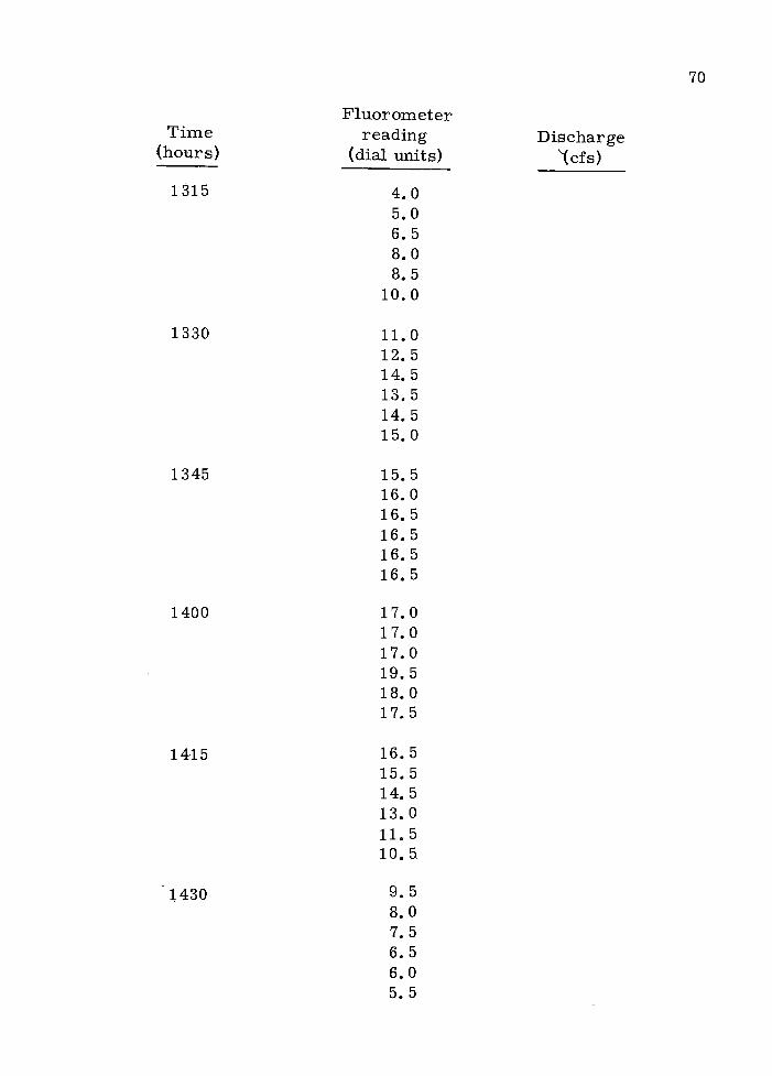
FluorometerTime reading Discharge

(hours) (dial units) (cfs)

1315 4.005

8. 08. 5

10. 0

1330

1345

1400

1415

1430

11.05

14.55

5

15.0

15.516. 016. 516. 516. 516.5

17.017.017.019. 518. 017.5

16. 55

14. 513. 011.510. 5

9. 58. 07. 56. 56. 05. 5

70

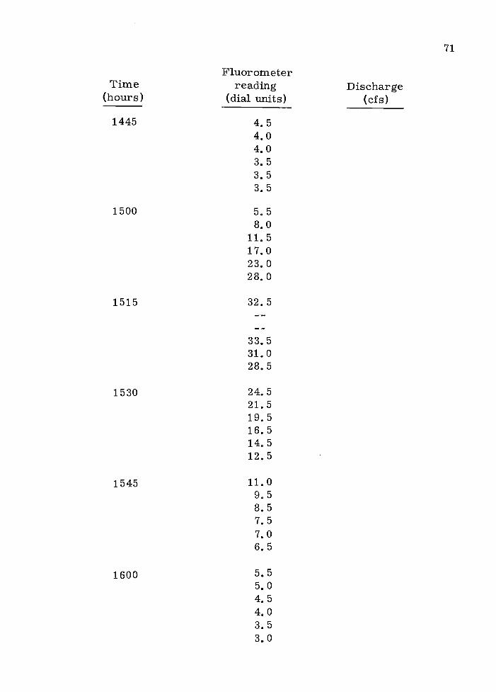
FluorometerTime reading Discharge

(hours) (dial units) (cfs)

1445 4.54. 04. 03. 53. 53. 5

1530

1545

1600

1515 32.5

33. 531.028. 5

24. 521.519. 516. 514. 512. 5

11.09. 58. 57. 57. 06. 5

5. 55. 04. 54. 03. 53. 0

71

1500 5. 58. 0

11.517.023. 028. 0

FluorometerTime reading Discharge

(hours) (dial units) (cis)

1615 2.52. 52.02. 0

1.5

1630 1.51.0

1645 0.0

72

APPENDIX BSABINO CREEK TEST

Fluorometer calibration: 9.5 ppb 25 on fluorometer dial.

Injection solution 2,730,000 ppb.

Injection rate = 13.17 ml per sec.

A smooth curve was passed through the plotted curve of the fluorometerreading versus time. The value in the "Average" column was takenfrom this curve.

Discharge obtained by current-meter measurements is listed as CMM.

A background of 1,0 dial units has been removed from the following data.

FluorometerTime reading Average Discharge

(hours) (dial units) (dial units) (cfs)

2145 0.00, 50. 00. 00. 51.5

73

2200 3. 55

5

11.512.016.0

74

Time(hours)

Fluorometerreading

(dial units)Average

(dial units)Discharge

(cfs)

2215 18.520. 020. 520. 521.021.0

2230 21.5 22. 0 151,921.5 22. 1 151.222. 5 22. 2 150.622. 5 22. 3 150.022.0 22. 4 149.422. 5 22. 5 148. 5

2245 23. 5 22. 6 148, 022. 5 22, 7 147,422. 5 22, 8 146, 723. 5 22. 9 146.022. 5 23, 0 145,322. 5 23. 0 145.3

2300 22. 5 23, 1 144. 723. 0 23, 2 144,123. 5 23, 3 143, 523. 5 23. 4 142,823. 5 23. 4 142. 823. 0 23. 5 142,3

2315 23. 5 23. 5 142.324, 0 23, 6 141.632. 0 23. 7 ç 141.0

148.0 CMM23. 5 23. 7 141,023. 5 23. 8 140, 123. 0 23. 8 140, 1

2330 23. 0 23. 9 139.824. 5 24. 0 139, 323. 5 24. 0 139,323. 5 24. 1 138. 723. 5 24. 1 138.723. 5 24, 1 138. 7

75

Time(hours)

Fluorometerreading

(dial units)Average

(dial units)Discharge

(cfs)

2345 24.0 24.2 138.123.5 24.2 138.123.5 24.3 137.524.5 24.3 137,524.5 24.3 137.524.5 24,4 137.0

2400 24. 5 24. 4 137. 024. 5 24. 4 137.024. 5 24. 5 136.424. 5 24. 5 136, 424. 5 24. 5 136.424. 5 24. 5 136. 4

2415 23. 522. 021.020. 015.012.5

2430 10.09. 05. 55. 53. 02. 5

2445 2. 51.50. 50. 00. 00. 0

0100 0. 0

APPENDIX CPARJA RIVER TEST

Fluorometer calibration: 29 ppb = 39.5 on fluorometer dial.

Injection solution = 1,740,000 ppb.

Injection rate = 4,22 ml per sec.

A smooth curve was passed through the plot of the fluorometer readingversus time, The value in the "Average" column was taken fromthis curve,

Discharge obtained by current-meter measurement is listed as CMM.

FluorometerTime reading Average Discharge

(hours) (dial units) (dial units) (cfs)

(Upper station)

76

1100 0. 00. 00. 51.05. 57. 5

1115 11.017.522. 531. 034. 539. 0

77

Time(hours)

Fluorometerreading

(dial units)Average

(dial units)Discharge

(cis)

1130 42.542. 548. 544. 549. 543. 0

1145 43. 543. 543. 042, 543. 541. 5

1200 40. 539. 5 39, 0 9.0639. 5 39, 0 900639. 0 39. 1 9.0443. 5 39. 1 9,0440. 0 39, 1 9.04

1215 39. 5 39, 2 9.0240. 0 39, 2 9.0239. 0 39. 2 9.0238. 5 39. 3 9.0043. 0 39. 3 9.0039. 5 39, 3 9,00

1230 38, 5 39. 4 8,9738. 5 39, 4 8, 9739, 5 39, 4 8.9739, 5 390 5 8.9440.0 39. 5 8.9439. 5 39. 5 8.94

1245 40, 0 39. 6 8.9239. 5 39. 6 8.9239, 5 39. 6 8.9239. 5 39. 7 8.9039. 5 39. 7 8.9039. 5 39, 7 8,90

78

Time(hours)

Fluorometerreading

(dial units)Average

(dial units)Discharge

(cfs)

1300 40.0 39.8 8.8839.5 39.8 8.8839.5 39.8 8.8840.5 39.9 8.8544.5 39,9 8.8539.5 39.9 8,85

1315 40. 5 40. 0 8. 8345.0 40. 0 8, 8339. 5 40. 0 8. 8341.0 40. 1 8.8140. 5 40. 1 8.8139. 5 40. 1 8. 81

1330 39. 5 40. 2 8. 7939. 038. 028. 528. 524. 5

1345 18.013.0

7. 07. 55. 52.0

1400 3. 02. 01.0 7.85 CMM1.01.00. 5

FluorometerTime reading Average Discharge

(hours) (dial units) (dial units) (ci s)

1200

1 ai 5

1230

1245

1300

0. 00. 50. 00. 00. 00. 5

0. 51.54. 06. 5

11.516. 0

20. 524. 028.534. 537. 541. 0

41. 042.043. 5

00

43. 5

46. 545. 5

5

5

45. 542. 5

(Lower station)

79

Fluoromet erTime reading Average Discharge

(hours) (dial units) (dial units) (cfs)

1315 41.541.541.541. 541. 544. 5

1330

1345

1400

1415

42, 542. 044. 542. 040. 540. 5

40. 55

5

041. 041,5

41. 544, 541, 540. 542. 0

5

046. 0

00

45. 544. 0

80

1430 43. 543.043. 541. 041. 5

APPENDIX DCHINLE WASH TEST

Fluorometer calibration: 108 ppb = 49,5 on fluorometer dial.

Injection solution 1,700,000 ppb.

Injection rate 4.22 ml per sec.

A smooth curve was passed through the plot of the fluorometer readingversus time, The value in the "Average" column was taken fromthis curve,

Fluorom et erTime reading Average Discharge

(hours) (dial units) (dial imits) (cfs)

1215

1230

1245

0.00. 00. 00. 00. 01.0

1.500005

05

11.513.015.017.0

81

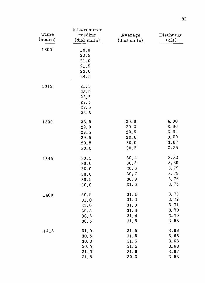
82

Time(hours)

Fluorometerreading

(dial units)Average

(dial units)Dis charge

(cfs)

1300 18.020. 521.021. 523. 024. 5

1315 25. 525. 526. 527.527. 528. 5

1330 28. 5 29. 0 4,0029.0 29. 3 3.9629. 5 29. 5 3.9429. 5 29. 8 3. 9029. 5 30. 0 3. 8730. 0 30. 2 3. 85

1345 30. 5 30. 4 3.8230. 0 30. 5 3.8030. 0 30. 6 3, 7930. 0 30. 7 3. 7830. 5 30. 9 3. 7630. 0 31. 0 3. 75

1400 30. 5 31. 1 3. 7331. 0 31. 2 3. 7231. 0 31. 3 3, 7130. 5 31. 4 3. 7030, 5 31. 4 3. 7030, 5 31. 5 3. 68

1415 31. 0 31. 5 3.6830. 5 31. 5 3,6830. 0 31. 5 3.6830. 5 31. 5 3.6831.0 31. 6 3.6731. 5 32. 0 3,63

83

Time(hours)

Fluorometerreading

(dial units)Average

(dial units)Discharge

(cfs)

1430 32. 5 33, 0 305233. 5 34. 0 3.4234. 0 34. 5 3. 3734. 5 35. 5 3.2835. 5 36. 5 3. 1937. 5 37. 2 3.13

1445 38. 5 38. 0 3.0739. 0 39. 0 3.0040. 5 40. 0 2.9240. 5 40. 6 2. 8741. 5 41. 5 2. 8142. 5 42. 5 2. 74

1500 43. 0 43. 2 2. 6945. 0 44. 0 2.6444. 5 45. 0 2.5846. 0 45. 7 2.5447. 0 46. 5 2.5046. 5 47. 5 2.45

1515 48. 0 48. 3 2.4048. 0490 5490 550. 050. 5

1530 50. 5

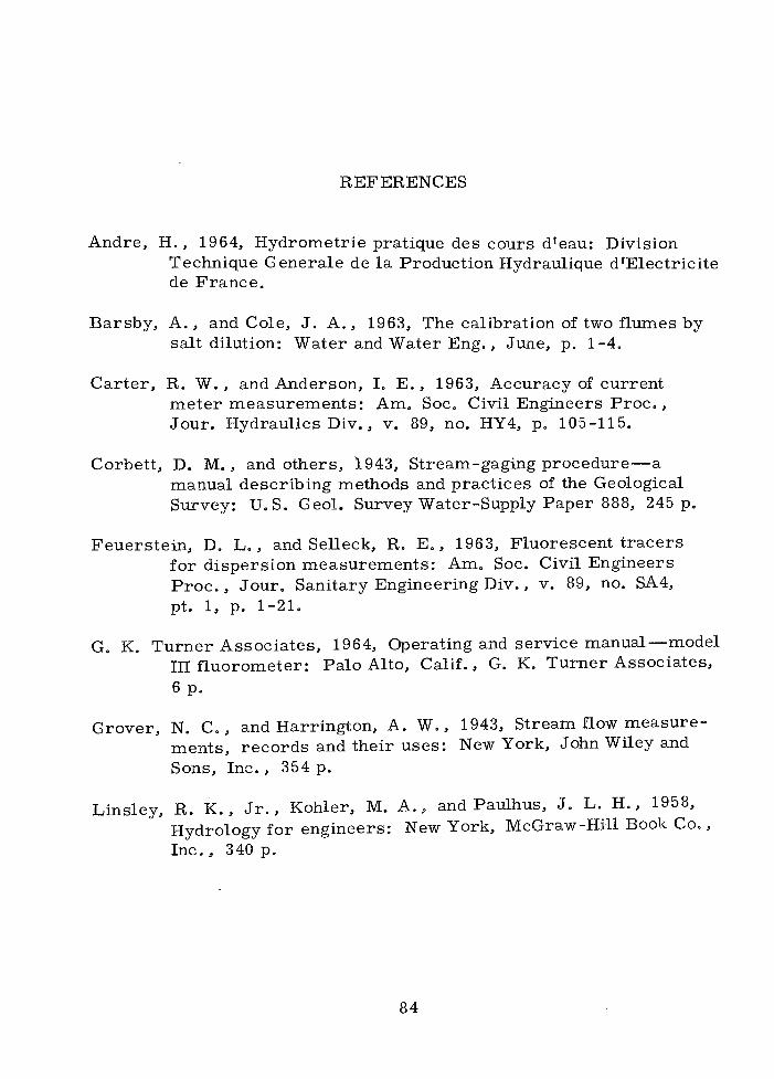
REF ERENCES

Andre, H., 1964, Hydrometrie pratique des cours dteau: DivisionTechnique Generale de la Production Hydraulique dtElectricitede France,

Barsby, A., and Cole, J. A., 1963, The calibration of two flumes bysalt dilution: Water and Water Eng., June, p. 1 -4.

Carter, R. W., and Anderson, I. E., 1963, Accuracy of currentmeter measurements: Am, Soc. Civil Engineers Proc.,Jour. Hydraulics Div., v. 89, no. HY4, p. 105-115.

Corbett, D. M., and others, 1943, Stream-gaging procedureamanual describing methods and practices of the GeologicalSurvey: U. S. Geol. Survey Water-Supply Paper 888, 245 p.

Feuerstein, D. L., and Selleck, R. E., 1963, Fluorescent tracersfor dispersion measurements: Am, Soc. Civil EngineersProc., Jour. Sanitary Engineering Div., v. 89, no. SA4,pt. 1, p. 1-21.

G. K. Turner Associates, 1964, Operating and service manualmodelIII fluorometer: Palo Alto, Calif., G. K. Turner Associates,6 p.

Grover, N. C., and Harrington, A. W., 1943, Stream flow measure-ments, records and their uses: New York, John Wiley andSons, Inc., 354p.

Linsley, R. K., Jr., Kohier, M. A., and Paulihus, J, L. H., 1958,Hydrology for engineers: New York, McGraw-Hill Book Co.,Inc., 340 p.

84

85

U. S. Bureau of Reclamation, Lynch Radiation Services, and Universityof California, 1961, Report on field demonstration use ofisotopes in hydrographic measurements, Gila Project,Arizona: U. S. Bur. Reclamation, duplicated report, 73 p.

U. S. Inter-Agency Committee on Water Resources, 1965, A study ofmethods used in measurement and analysis of sediment loadsin streams: Minneapolis, Minn., St. Anthony Falls HydraulicLab., Report J, 5 p.

Wright, R. R., and Collings, M. R,, 1964, Application of fluorescenttracing techniques to hydrologic studies: Am. Water WorksAssoc. Jour., v. 56, no. 6, p. 748-754.