wild bootstrap for instrumental variables regressions with
TRANSCRIPT
Wild Bootstrap for Instrumental Variables Regressionswith Weak and Few Clusters∗
Wenjie Wang† and Yichong Zhang‡
November 25, 2021
Abstract
We study the wild bootstrap inference for instrumental variable (quantile) regressions in theframework of a small number of large clusters, in which the number of clusters is viewed as fixedand the number of observations for each cluster diverges to infinity. For subvector inference, weshow that the wild bootstrap Wald test with or without using the cluster-robust covariance matrixcontrols size asymptotically up to a small error as long as the parameters of endogenous variablesare strongly identified in at least one of the clusters. We further develop a wild bootstrap Anderson-Rubin (AR) test for full-vector inference and show that it controls size asymptotically up to a smallerror even under weak or partial identification for all clusters. We illustrate the good finite-sampleperformance of the new inference methods using simulations and provide an empirical applicationto a well-known dataset about U.S. local labor markets.
Keywords: Wild Bootstrap, Weak Instrument, Clustered Data, Randomization Test, InstrumentalVariable Quantile Regression.
JEL codes: C12, C26, C31
1 Introduction
Various recent surveys on leading economic journals suggest that weak instruments remain
important concerns for empirical practice. For instance, Andrews, Stock, and Sun (2019) survey
230 instrumental variable (IV) regressions from 17 papers published in the American Economic
Review (AER). They find that many of the first-stage F -statistics (and nonhomoskedastic
generalizations) are in a range that raise such concerns, and virtually all these papers reported at
least one first-stage F with value smaller than 10. Brodeur, Cook, and Heyes (2020) investigate
∗We are grateful to Aureo de Paula, Firmin Doko Tchatoka, Kirill Evdokimov, Qingfeng Liu, Ryo Okui, Kevin Song,Naoya Sueishi, Yoshimasa Uematsu, and participants at the 2021 Annual Conference of the International Association forApplied Econometrics, the 2021 Asian Meeting of the Econometric Society, the 2021 China Meeting of the EconometricSociety, the 2021 Australasian Meeting of the Econometric Society and the 2021 Econometric Society European Meetingfor their valuable comments. Wang acknowledges the financial support from NTU SUG Grant No.M4082262.SS0. Zhangacknowledges the financial support from Singapore Ministry of Education Tier 2 grant under grant MOE2018-T2-2-169and the Lee Kong Chian fellowship. Any possible errors are our own.
†Division of Economics, School of Social Sciences, Nanyang Technological University. HSS-04-65, 14 Nanyang Drive,Singapore 637332. E-mail address: [email protected].
‡School of Economics, Singapore Management University. E-mail address: [email protected].
1
arX
iv:2
108.
1370
7v1
[ec
on.E
M]
31
Aug
202
1

p-hacking and publication bias among over 21,000 hypothesis tests in 25 leading economic
journals. They notice, in IV regressions, a sizable over-representation of first-stage F just over
10 (also observed in Andrews et al. (2019)), and studies with relatively weak instruments have
a much higher proportion of second-stage t-statistics barely significant around 1.65 and 1.96.
The issue of weak instruments is further complicated by the fact that in many empirical
settings, observations are clustered and the number of clusters is small (e.g., when clustering
is based on states, provinces, neighboring countries or industries). In such case, the commonly
employed cluster-robust covariance estimator (CCE) is no longer consistent even under strong
instruments, and cluster-robust first-stage F test (Olea and Pflueger, 2013) cannot be directly
applied as its critical values are obtained under the asymptotic framework with a large number
of clusters. Recently, Young (2021) analyzes 1359 IV regressions in 31 papers published by the
American Economic Association (AEA), and highlights that many findings rest upon unusually
large values of test statistics (rather than coefficient estimates) due to inaccurate estimates of
covariance matrices, and are highly sensitive to influential clusters or observations : with the
removal of just one cluster or observation, in the average paper the first-stage F can decrease
by 28%, and 38% of reported 0.05 significant two-stage least squares (TSLS) results can be
rendered insignificant at that level, with the average p-value rising from 0.029 to 0.154.
Motivated by these issues, we study wild bootstrap inference for linear IV and IV quantile
regressions (IVQR) with a small number of clusters by exploiting its connection with a ran-
domization test based on the group of sign changes, following the lead of Canay, Santos, and
Shaikh (2020). First, for both IV and IVQR, we show that subvector inference based on a wild
bootstrap Wald test with or without CCE controls size asymptotically up to a small error, as
long as there exists at least one strong cluster, in which the parameters of endogenous variables
are strongly identified. We further establish conditions under which they have power against
local alternatives (e.g., at least 5 strong clusters are required when the total number of clusters
equals 10 and the nominal level α equals 10%). Second, for IV and IVQR, we develop full-
vector inference based on a wild bootstrap Anderson and Rubin (1949, AR) test, which controls
size asymptotically up to a small error regardless of instrument strength. Additionally, for IV
regressions the wild bootstrap Wald test without CCE is numerically equivalent to certain wild
bootstrap AR test in the empirically prevalent case with single IV,implying that it is robust to
weak identification. Third, for IV regressions we establish the validity result for bootstrapping
weak-IV-robust tests other than the AR test with at least one strong cluster. Fourth, to pro-
vide subvector and full-vector inference for IVQR with a small number of clusters, we propose
a novel two-step gradient wild bootstrap procedure.
Our approach has several empirically relevant advantages. First, it enhances practitioners’
toolbox by providing reliable inference for IV and IVQR with a small number of clusters, as
2

illustrated by our study on the average and distributional effects of Chinese imports on local
labor markets in different US regions, following Autor, Dorn, and Hanson (2013). Second, it
is flexible with IV strength: by allowing for cluster-level heterogeneity in the first stage, the
bootstrap Wald test is robust to influential clusters, while its AR counterpart is fully robust
to weak instruments. Third, different from widely used heteroskedasticity and autocorrela-
tion consistent (HAC) estimators, our approach is agnostic about within-cluster dependence
structure and thus avoids the use of tuning parameters to estimate the covariance matrix.
The contributions in the present paper relate to several strands of literature. First, it is
related to the literature on cluster-robust inference.1 Djogbenou et al. (2019), MacKinnon
et al. (2019) and Menzel (2021) show bootstrap validity under the asymptotic framework with
a large number of clusters. However, as emphasized by Ibragimov and Muller (2010, 2016),
Bester, Conley, and Hansen (2011), Cameron and Miller (2015), Canay, Romano, and Shaikh
(2017), Hagemann (2019a,b, 2020) and Canay et al. (2020), many empirical studies motivate an
alternative framework in which the number of clusters is small, while the number of observations
in each cluster is relatively large. For inference, we may consider applying the approaches
developed by Bester et al. (2011), Hwang (2020), Ibragimov and Muller (2010, 2016), and
Canay et al. (2017). However, Bester et al. (2011) and Hwang (2020) require (asymptotically)
equal cluster-level sample size, while Ibragimov and Muller (2010, 2016) and Canay et al. (2017)
hinge on strong identification for all clusters. Our bootstrap Wald test is more flexible as it
does not require equal cluster size and only needs strong identification in one of the clusters.
Second, our paper is related to the literature on weak IVs, and various normal approximation-
based inference approaches are available for non-homoskedastic cases, among them Stock and
Wright (2000), Kleibergen (2005), Andrews and Cheng (2012), Andrews (2016), Andrews and
Mikusheva (2016), Andrews (2018), Moreira and Moreira (2019) and Andrews and Guggen-
berger (2019). As remarked by Andrews et al. (2019, p.750), an important question concerns
the quality of normal approximation with influential observations or clusters. When imple-
mented appropriately, bootstrap may substantially improve inference for IV regressions2 and
Moreira et al. (2009) establish validity of bootstrap weak-IV-robust tests under weak IVs and
homoskedasticity. While it is possible to extend their results by allowing the number of clusters
to tend to infinity, such a framework could be unreasonable with influential clusters. We com-
plement this approach by establishing validity for these tests under the alternative asymptotics.
1See Cameron, Gelbach, and Miller (2008), Conley and Taber (2011), Imbens and Kolesar (2016), Abadie, Athey,
Imbens, and Wooldridge (2017), Hagemann (2017, 2019a,b, 2020), MacKinnon and Webb (2017), Djogbenou, MacKinnon,
and Nielsen (2019), MacKinnon, Nielsen, and Webb (2019), Ferman and Pinto (2019), Hansen and Lee (2019), Menzel
(2021), among others, and MacKinnon, Nielsen, and Webb (2020) for a recent survey.2See, e.g., Davidson and MacKinnon (2010), Moreira, Porter, and Suarez (2009), Wang and Kaffo (2016), Finlay and
Magnusson (2019), and Young (2021), among others.
3
Third, our paper is related to the literature on IVQR.3 Although IVQR can be estimated
via GMM, for computational feasibility, we follow Chernozhukov and Hansen (2006) and im-
plement a profiled estimation procedure, which falls outside the scope of wild bootstrap for
GMM outlined by Canay et al. (2020). For subvector inference, our gradient wild bootstrap
procedure is similar to the one implemented by Hagemann (2017) for linear quantile regression
with clustered data and Jiang, Liu, Phillips, and Zhang (2020) for quantile treatment effect
estimation in randomized control trials, but it imposes null hypothesis and further involves a
profiled minimization to obtain the bootstrap IVQR estimator. Also different from the two
papers, we show bootstrap validity by connecting it to the randomization test. For full-vector
inference, we follow the idea by Chernozhukov and Hansen (2008) and complement their results
by considering the setup with a small number of large clusters and proposing a wild bootstrap
AR test for IVQR.
Finally, we notice that although empirical applications often involve settings with substantial
first-stage heterogeneity, related econometric literature remains rather sparse. Abadie, Gu, and
Shen (2019) exploits such heterogeneity to improve the asymptotic mean squared error of IV
estimators in the homoskedastic case. Instead, we focus on developing inference methods that
are robust to the first-stage heterogeneity for both IV and IVQR with clustered data.
The remainder of this paper is organized as follows. Sections 2 and 3 present the main
results for IV and IVQR, respectively. Section 4 discusses cluster-level variables. Section 5
provides simulation results and practical recommendations. Section 6 presents the empirical
application.
2 Linear IV Regression
In this section, we consider a setup of linear IV model with clustered data,
yi,j = X>i,jβ +W>i,jγ + εi,j, Xi,j = Z>i,jΠz,j +W>
i,jΠw + vi,j, (1)
where the clusters are indexed by j ∈ J ≡ 1, ..., q and units in the j-th cluster are indexed
by i ∈ In,j ≡ 1, ..., nj. yi,j ∈ R, Xi,j ∈ Rdx , Wi,j ∈ Rdw , and Zi,j ∈ Rdz denote an outcome
of interest, endogenous regressors, exogenous regressors, and IVs, respectively. β ∈ Rdx and
γ ∈ Rdw are unknown structural parameters, while Πz,j ∈ Rdz×dx and Πw ∈ Rdz×dw are
unknown parameters of the first stage. We allow for cluster-level heterogeneity with regard to
IV strength by letting Πz,j in (1) to vary across clusters. This setting is motivated by the fact
that in empirical studies IVs are often strong for some subgroups and weak for some others, such
as ethnic groups and geographic regions (Abadie et al., 2019), and, as noted previously, many
3See, e.g., Chernozhukov and Hansen (2004, 2005, 2006, 2008), Wuthrich (2019), Chernozhukov, Hansen, and
Wuthrich (2020), and Kaido and Wuthrich (2021) for a comprehensive literature review.
4

TSLS estimates and first-stage F s are highly sensitive to influential clusters. Furthermore, in
experimental economics with clustered randomized trials, subjects’ compliance with assignment
may also have substantial variations among clusters, resulting in heterogenous IV strength.4
We next introduce the assumptions that will be used in our analysis of the asymptotic
properties of the wild bootstrap tests under a small number of clusters.
Assumption 1. The quantities
1√n
∑j∈J
∑i∈In,j
(Zi,jεi,j
Wi,jεi,j
),
1
n
∑j∈J
∑i∈In,j
(Zi,jZ
>i,j Zi,jW
>i,j
Wi,jZ>i,j Wi,jW
>i,j
), and
1
n
∑j∈J
∑i∈In,j
(Zi,jX
>i,j
Wi,jX>i,j
)converges in distribution, converges in probability to a positive-definite matrix, and converges
in probability to a full rank matrix, respectively.
Assumption 2. The following statements hold:
(i) There exists a collection of independent random variables Zj : j ∈ J, where Zj ≡ [Zε,j :
Zv,j] with Zε,j ∈ Rdz and Zv,j ∈ Rdz×dx, and vec(Zj) ∼ N(0,Σj) with Σj positive definite for
all j ∈ J , such that 1√nj
∑i∈In,j
Zi,jεi,j,1√nj
∑i∈In,j
Zi,jv>i,j
: j ∈ J
d−−→ Zj : j ∈ J .
(ii) For each j ∈ J , nj/n→ ξj > 0.
(iii) 1n
∑j∈J∑
i∈In,j Wi,jW>i,j is invertible.
(iv) For each j ∈ J ,
1
nj
∑i∈In,j
∥∥∥W>i,j
(Γn − Γcn,j
)∥∥∥2 P−−→ 0,
where Γn and Γcn,j denotes the coefficient from linearly regressing Zi,j on Wi,j by using the entire
sample and by only using the sample in the j-th cluster, respectively.
Remark 1. The above assumptions are similar to those imposed in Canay et al. (2020). As-
sumption 1 ensures that the TSLS estimators (and their null-restricted counterparts) are well
behaved. Assumption 2(i) is satisfied whenever the within-cluster dependence is sufficiently
weak to permit application of a suitable central limit theorem and the data are independent
across clusters. The assumption that Zj have full rank covariance matrices requires that Zi,j
can not be expressed as a linear combination of Wi,j within each cluster j. Assumption 2(ii)
gives the restriction on cluster sizes. Assumption 2(iii) ensures Γn is uniquely defined. Assump-
tion 2(iv) is the sufficient condition for 1nj
∑i∈In,j Zi,jW
>i,j = op(1), which is needed in our proof.
4E.g., in Muralidharan, Niehaus, and Sukhtankar (2016)’s evaluation of a smartcard payment system, in some villages
90% or more of the recipients complied with the treatment assignment, while in many villages less than 10% complied.
5

It holds under cluster homogeneity. As pointed out by Canay et al. (2020), this assumption is
satisfied whenever the distributions of (Z>i,j,W>i,j)> are the same across clusters. Furthermore,
Assumption 2(iv) holds automatically if Wi,j includes cluster dummies and their interactions
with all other control variables. If Wi,j includes cluster-level variables, then including cluster
dummies would violate Assumption 2(iii). In Section A of the Online Supplement, we propose
a cluster-level projection procedure, which ensures 1nj
∑i∈In,j Zi,jW
>i,j = 0 for j ∈ J .
2.1 Subvector Inference
In this section, we study the properties of the wild bootstrap test based on IV estimates under
the asymptotic framework where the number of clusters is kept fixed. We let the parameter of
interest β to shift w.r.t. the sample size to incorporate the analyses of size and local power in a
concise manner: βn = β0 +µβ/√n, where µβ ∈ R is the local parameter. Let λ>β β0 = λ0, where
λβ ∈ Rdx×dr , λ0 ∈ Rdr×1 and dr denotes the number of restrictions under the null hypothesis.
Define µ = λ>β µβ. Then, the null and local alternative hypotheses can be written as
H0 : µ = 0 v.s. H1,n : µ 6= 0. (2)
We consider the test statistic with a dr × dr weighting matrix Ar, i.e.,
Tn ≡ ||√n(λ>β β − λ0)||Ar , (3)
where ||u||A =√u>Au for a generic vector u and a weighting matrix A. The wild bootstrap
test is implemented as follows:
Step 1: Compute the null-restricted residual εri,j = yi,j − X>i,jβr − W>
i,j γr, where βr and γr are
null-restricted two-stage least squares estimators of β and γ.
Step 2: Let G = −1, 1q and for any g = (g1, ..., gq) ∈ G generate
y∗i,j(g) = X>i,jβr +W>
i,j γr + gj ε
ri,j. (4)
For each g = (g1, ..., gq) ∈ G compute β∗g and γ∗g , the analogues of the two-stage least
squares estimators β and γ using y∗i,j(g) in place of yi,j and the same (Z>i,j, X>i,j,W
>i,j)>.
Compute the bootstrap analogues of test statistic:
T ∗n(g) = ||√n(λ>β β
∗g − λ0)||A∗r,g , (5)
where A∗r,g denotes the bootstrap weighting matrix, which will be specified below.
Step 3: To obtain the critical value, we compute the 1− α quantile of T ∗n(g) : g ∈ G:
cn(1− α) ≡ inf
x ∈ R :
1
|G|∑g∈G
IT ∗n(g) ≤ x ≥ 1− α
, (6)
6

where IE equals one whenever the event E is true and equals zero otherwise. The
bootstrap test for H0 rejects whenever Tn exceeds cn(1− α).
Let QZX,j = n−1j
∑i∈In,j Zi,jX
>i,j and QZX = n−1
∑j∈J∑
i∈In,j Zi,jX>i,j, where Zi,j is the
residuals from regressing Zi,j on Wi,j using full sample, i.e., Zi,j = Zi,j − Γ>nWi,j and Γn is
defined in Assumption 2(iv). Let QZX,j and QZX denote the probability limits of QZX,j and
QZX , respectively. In addition, let QZZ = n−1∑
j∈J∑
i∈In,j Zi,jZ>i,j, Q = Q>
ZXQ−1
ZZQZX , and let
QZZ and Q denote the probability limits of QZZ and Q, respectively.
Assumption 3. One of the following two conditions holds: (i) dx = 1 and (ii) There exists a
scalar aj for each j ∈ J such that QZX,j = ajQZX .
Assumption 3(i) states that in the case with one endogenous variable (the leading case in em-
pirical applications), no further condition is required. In this case, we let aj = Q−1Q>ZXQZZQZX,j.
With multiple endogenous variables, Assumption 3(ii) requires that QZX,j = ajQZX for all
j ∈ J , where aj 6= 0 for some clusters and aj = 0 otherwise. Assumption 1 ensures that overall
we have strong identification, and thus, QZX is of full rank, then when aj 6= 0, QZX,j is also of
full rank, i.e., the coefficients of the endogenous variables βn are strongly identified in cluster
j. We call these clusters the strong clusters. On the other hand, strong identification for βn is
not ensured in the rest clusters. For these clusters, Assumption 3(ii) excludes the case that the
Jacobian matrix QZX,j is of reduced rank but not a zero matrix.5
We first study the asymptotic behaviours of the wild bootstrap Wald test when the weighting
matrix Ar in (3) has a deterministic limit and the bootstrap weighting matrix A∗r,g equals Ar.
Assumption 4. ||Ar−Ar||op = op(1), where Ar is a dr×dr symmetric deterministic weighting
matrix such that 0 < c ≤ λmin(Ar) ≤ λmax(Ar) ≤ C < ∞ for some constants c and C, where
λmin(A) and λmax(A) are the minimum and maximum eigenvalues of the generic matrix A.
Theorem 2.1. (i) Suppose that Assumptions 1-4 hold. Then under H0,
α− 1
2q−1≤ lim inf
n→∞PTn > cn(1− α) ≤ lim sup
n→∞PTn > cn(1− α) ≤ α.
(ii) Further suppose that there exists a subset Js of J such that aj > 0 for each j ∈ Js, aj = 0
for j ∈ J\Js, and d|G|(1− α)e ≤ |G| − 2q−qs+1, where qs = |Js|. Then under H1,n,
lim||µ||2→∞
lim infn→∞
PTn > cn(1− α) = 1.
Remark 2. Theorem 2.1 states that as long as there exists at least one strong cluster, the Tn-
based wild bootstrap test is valid in the sense that its limiting null rejection probability is no
5It is possible to select out the clusters with Jacobian matrices of reduced rank via some testing procedure (Robin
and Smith, 2000; Kleibergen and Paap, 2006; Chen and Fang, 2019). We leave this investigation for future research.
7

greater than the nominal level α, and no smaller than α−1/2q−1, which decreases exponentially
with the total number of clusters rather than the number of strong clusters. Intuitively, although
the weak clusters do not contribute to the identification of βn, the scores of such clusters and
their bootstrap counterparts (i.e., 1√nj
∑i∈In,j Zi,jεi,j and 1√
nj
∑i∈In,j gjZi,j ε
ri,j for j ∈ J\Js) still
contribute to the limiting distribution of TSLS and the randomization with sign changes.
Additionally, one might consider employing an alternative procedure (e.g., see Moreira et al.
(2009), Davidson and MacKinnon (2010), Finlay and Magnusson (2019) and Young (2021)):
X∗i,j(g) = Z>i,jΠz +W>i,jΠw + gj vi,j, y∗i,j(g) = X∗>i,j (g)βr +W>
i,j γr + gj ε
ri,j, (7)
where Πz and Πw are some estimates of the first-stage coefficients. This procedure is asymp-
totically equivalent to ours under the current framework.
Remark 3. Theorem 2.1 also can be shown for other IV estimators such as the limited infor-
mation maximum likelihood (LIML) and jackknife IV estimators (JIVEs). For instance, let
(β>liml, γ>liml)
> = (X>PZX − µX>MZX)−1(X>PZY − µX>MZY ), (8)
where µ = minr r>Y >MWZ(Z>MWZ)−1Z>MW Y r/(r
>Y >MZ Y r), r = (1,−β>)>, Y = [Y :
X], Z = [Z : W ], X = [X : W ], Y , ε, X, Z and W are formed by yi,j, εi,j, X>i,j, Z
>i,j and W>
i,j,
respectively, and PA = A(A>A)−1A>, MA = In − PA, where A is a n-dimensional matrix and
In is a n-dimensional identity matrix. Then, by the definition of µ,
nµ ≤(
1√ne>MWZ
)(1
nZ>MWZ
)−1(1√nZ>MW e
)/
(1
ne>MZe
)= OP (1), (9)
and LIML has the same limiting distribution as TSLS under Assumptions 1 and 2. The results
in Theorem 2.1 therefore hold for the wild bootstrap test with LIML as well. We omit the
details for brevity but notice that LIML is less biased than TSLS in the over-identified case6
and its corresponding bootstrap tests can therefore have better finite-sample size control since
the randomization requires distributional symmetry around zero (see Section 5.1).
Remark 4. For the empirically prevalent case with single endogenous variable and single IV
(e.g., 101 out of 230 specifications in Andrews et al. (2019)’s sample and 1087 out of 1359 in
Young (2021)’s sample), the Tn-based wild bootstrap test is numerically equivalent to certain
bootstrap AR test (the ARn-based bootstrap test in Section 2.2), which is fully robust to
weak IV. However, the more widely used wild bootstrap test with CCE (e.g., Cameron et al.
(2008), Cameron and Miller (2015), and Roodman, Nielsen, MacKinnon, and Webb (2019)) is
not weak-IV robust and thus may produce size distortions in this case, if the IV is weak (see
Section 5.1). Furthermore, the robustness depends on our specific procedure and thus cannot
6It may be interesting to consider an alternative asymptotic framework in which the number of clusters is fixed but
the number of IVs tends to infinity (Bekker, 1994). We leave this direction of investigation for future research.
8

be extended to alternative ones such as the commonly employed pairs cluster bootstrap (block
bootstrap, e.g., see Angrist and Pischke (2008), Goldsmith-Pinkham, Sorkin, and Swift (2020),
and Hahn and Liao (2021); including percentile, percentile-t and bootstrap standard error).
Remark 5. For alternative inference methods with a small number of clusters, Bester et al.
(2011) and Hwang (2021) provide asymptotic approximations that are based on t and F distri-
butions, in the spirit of Kiefer and Vogelsang (2002, 2005)’s fixed-k asymptotics. Their approach
would require stronger homogeneity conditions than the wild bootstrap in the current context;
e.g., the cluster sizes are approximately equal for all clusters (nj/n → 1 for j ∈ J , where
n = q−1∑
j∈J nj), the cluster-level scores in Assumption 2(i) have the same normal limiting
distribution for all clusters, and the cluster-level Jacobian matrices in Assumption 3 have the
same probability limit for all strong clusters, i.e., aj = 1 for j ∈ Js.Furthermore, the wild bootstrap test has remarkable resemblance to the Fama-Macbeth type
approach in Ibragimov and Muller (2010, IM) and the randomization test with sign changes
in Canay et al. (2017, CRS), which are based on the asymptotic independence of cluster-level
estimators (say, β1, ..., βq). However, we notice that for IV regressions (and IVQR), their size
properties can be very different. For instance, IM and CRS rule out weak IVs in the sense
of Staiger and Stock (1997) for all clusters (i.e., Πz,j = n−1/2j Cj, where Cj has a fixed full
rank value), as the cluster-level IV estimators of such weak clusters would become inconsistent
and have highly non-standard limiting distributions, violating their underlying assumptions.7
By contrast, the size result in Theorem 2.1 holds even with only one strong cluster. In this
sense, the wild bootstrap is more robust to cluster heterogeneity in IV strength. However, if
all clusters are strong and the cluster-level estimators have minimal finite-sample bias, IM and
CRS have advantage over the wild bootstrap as they do not require Assumption 3(ii) when
dx > 1. The two types of approaches could therefore be considered as complements.
Remark 6. To establish in Theorem 2.1 the power of the wild bootstrap test against n−1/2-
local alternatives, we need enough number of strong clusters and homogeneity of the signs of
Jacobians for these strong clusters.8 For instance, if q equals 10, the condition d|G|(1− α)e ≤|G| − 2q−qs+1 requires that qs ≥ 5 and qs ≥ 6 for α = 10% and 5%, respectively. Theorem 2.1
suggests that although the size of the test is well-controlled even when some clusters are weak,
to enhance power, it might be beneficial to merge some less influential clusters.9
7Also, if there exist both strong and “semi-strong” clusters, in which (unknown) convergence rates of IV estimators
can vary among clusters and be slower than√nj (Andrews and Cheng, 2012), then the estimators with slowest rate will
dominate in their statistics.8For the case with single IV, it requires Πz,j to have the same sign across all clusters. With one endogenous variable
and multiple (orthogonalized) IVs, it requires the sign of each element of Πz,j to be the same across all clusters.9To avoid double dipping, we need prior knowledge of cluster-level first-stage heterogeneity. For instance, as remarked
by Abadie et al. (2019), the return-to-schooling literature has often used compulsory schooling year as an IV for years
of schooling while minimum school-leaving age is determined by state-specific laws, and in studies that use exogenous
9

Now we consider wild bootstrap test for the Wald statistic when the weighting matrix Ar
equals Ar,CR, the inverse of CCE, where
Ar,CR =(λ>β V λβ
)−1
, (10)
V = Q−1Q>ZXQ−1
ZZΩQ−1
ZZQZXQ
−1, Q = Q>ZXQ−1
ZZQZX , QZZ = n−1
∑j∈J∑
i∈In,j Zi,jZ>i,j, Ω =
n−1∑
j∈J∑
i∈In,j
∑k∈In,j Zi,jZ
>k,j εi,j εk,j, εi,j = yi,j − X>i,jβ −W>
i,j γ, and β and γ are the TSLS
estimators. The corresponding Wald statistic is defined as
TCR,n = ||√n(λ>β β − λ0)||Ar,CR . (11)
We follow a similar wild bootstrap procedure by defining
T ∗CR,n(g) = ||√n(λ>β β
∗g − λ0)||A∗r,CR,g , A∗r,CR,g =
(λ>β V
∗g λβ
)−1
, (12)
where V ∗g = Q−1Q>ZXQ−1
ZZΩ∗CR,gQ
−1
ZZQZXQ
−1, Ω∗CR,g = n−1∑
j∈J∑
i∈In,j
∑k∈In,j Zi,jZ
>k,j ε∗i,j(g)ε∗k,j(g),
and ε∗i,j(g) = y∗i,j(g) − X>i,jβ∗g −W>i,j γ∗g . The bootstrap critical value cCR,n(1 − α) is the 1 − α
quantile of T ∗CR,n(g) : g ∈ G. The asymptotic behaviour of this test is given as follows.
Theorem 2.2. (i) Suppose that Assumptions 1-3 hold, and q > dr. Then under H0,
α− 1
2q−1≤ lim inf
n→∞PTCR,n > cCR,n(1− α) ≤ lim sup
n→∞PTCR,n > cCR,n(1− α) ≤ α +
1
2q−1.
(ii) Further suppose that there exists a subset Js of J such that minj∈Js |aj| > 0, aj = 0 for each
j ∈ J\Js, and d|G|(1− α)e ≤ |G| − 2q−qs+1, where qs = |Js|. Then under H1,n,
lim||µ||2→∞
lim infn→∞
PTCR,n > cCR,n(1− α) = 1.
Remark 7. Theorem 2.2 states that with at least one strong cluster, the TCR,n-based wild
bootstrap test controls size asymptotically up to a small error, and it has power against local
alternatives if the condition on the number of strong clusters is satisfied. Moreover, different
from Theorem 2.1, the power result in Theorem 2.2 does not require the homogeneity condition
on the sign of first-stage coefficients. Indeed, the critical values of the two tests have different
asymptotic behaviours, with cn(1−α)p−→∞ while cCR,n(1−α) = OP (1), as ||µ||2 →∞, which
translates into relatively good power properties of the bootstrap test with CCE. In particular,
we note that when dr = 1, its local power is strictly higher when ||µ||2 is sufficiently large.10
shock to oil or coal supply as an IV, states with large shares of oil or coal industries typically have strong first stage.10Note that as ||µ||2 →∞, lim infn→∞ PTCR,n > cCR,n(1−α) > lim infn→∞ P|
√n(λ>β β−λ0)|/λ>β V λβ > cn(1−α)
= lim infn→∞ PTn > cn(1 − α), where cn(1 − α) denotes the (1 − α) quantile of |√n(λ>β β
∗g − λ0)|/λ>β V λβ : g ∈ G,
and the inequality holds because cn(1− α)p−→∞, since λ>β V λβ = OP (1).
10

2.2 Full-vector Inference
In general, Theorems 2.1 and 2.2 do not hold when all clusters are “weak”. For instance, under
the weak-IV sequence such that Πz,j = n−1/2j Cj with some fixed full rank Cj for all j ∈ J ,
1√n
∑j∈J
∑i∈In,j
Zi,jX>i,j
d−−→∑j∈J
√ξjQZZ,jCj +
∑j∈J
√ξjZv,j, (13)
where QZZ,j = plim 1nj
∑i∈In,j Zi,jZ
>i,j and
∑j∈J√ξjQZZ,jCj, the signal part of the first stage,
is of the same order of magnitude as the noise part∑
j∈J√ξjZv,j. Then, the randomization with
sign changes would be invalid because for each j ∈ J , (i) the distribution of√ξj(QZZ,jCj + Zv,j
)is not symmetric around zero and (ii) Cj cannot be consistently estimated; e.g., for the boot-
strap analogue of (13), the procedure in (7) would result in the following limiting distribution:
∑j∈J
√ξjQZZ,jCj +
∑j∈J
√ξjgjZv,j +
∑j∈J
ξj(1− gj)QZZ,jQ−1
ZZ
∑j∈J
√ξjZv,j
, (14)
where the second term equals the G-transformed noise in (13) while the third is an extra term.
In the case that the parameter of interest may be weakly identified in all clusters or the
homogeneity condition in Assumption 3(ii) may not hold, we may consider inference on the full
vector of βn. Recall that βn = β0 + µβ/√n. Under the null, we have µβ = 0, or equivalently,
βn = β0. Define the AR statistic with an asymptotically deterministic weighting matrix as
ARn =∥∥√nf∥∥
A, (15)
where f = n−1∑
j∈J∑
i∈In,j fi,j, fi,j = Zi,j(yi,j −X>i,jβ0 −W>
i,j γr), γr is the null-restricted least
squares estimator of γ, i.e., γr =(∑
j∈J∑
i∈In,j Wi,jW>i,j
)−1∑j∈J∑
i∈In,j Wi,j(yi,j−X>i,jβ0), and
A is a dz×dz weighting matrix with asymptotically deterministic limit. Additionally, we define
the AR statistic with (null-imposed) CCE as
ARCR,n =∥∥√nf∥∥
ACR, ACR =
n−1∑j∈J
∑i∈In,j
∑k∈In,j
fi,jf>k,j
−1
. (16)
Another AR statistic widely applied in the literature is based on the reduced form of (1):11
ARR,n =∥∥√nδ∥∥
AR, AR =
(Q−1
ZZΩRQ
−1
ZZ
)−1
, (17)
where ΩR = n−1∑
j∈J∑
i∈In,j
∑k∈In,j Zi,jZ
>k,jui,juk,j, ui,j is the residual of regressing yi−X>i β0
on Zi,j and Wi,j, and δ is the corresponding least squares estimate of the coefficient of Zi,j. Our
bootstrap procedure is defined as follows.
11E.g., see Cameron and Miller (2015), Andrews et al. (2019), Roodman et al. (2019).
11

Step 1: Compute the null-restricted residual εri,j = yi,j −X>i,jβ0 −W>i,j γ
r.
Step 2: Let G = −1, 1q and for any g = (g1, ..., gq) ∈ G define
f ∗g = n−1∑j∈J
∑i∈In,j
f ∗i,j(gj), δ∗g = Q−1
ZZf ∗g , (18)
where f ∗i,j(gj) = Zi,jε∗i,j(gj), ε
∗i,j(gj) = gj ε
ri,j and u∗i,j(gj) equals the residual of regress-
ing ε∗i,j(gj) on Zi,j and Wi,j. Compute the bootstrap statistics: AR∗n(g) =∥∥√nf ∗g∥∥A,
AR∗CR,n(g) =∥∥√nf ∗g∥∥ACR , and AR∗R,n(g) =
∥∥√nδ∗g∥∥AR .Step 3: Let cAR,n(1 − α), cAR,CR,n(1 − α), and cAR,R,n(1 − α) denote the (1 − α)-th quantile of
AR∗n(g)g∈G, AR∗CR,n(g)g∈G and AR∗R,n(g)g∈G, respectively.
Remark 8. Unlike the Wald test in Section 2.1, we do not need to bootstrap the CCEs for
the AR test even though it also admits a random limit. This is because here we use the true
parameter value under the null instead of its estimator to compute the covariance matrix.
When the estimator is used (as in the Wald test), there is extra randomness that needs to be
replicated by the bootstrap. Such randomness is gone when the true parameter value is used.
Theorem 2.3 shows that in the general case with multiple IVs, the ARn-based bootstrap
test is fully robust to weak IVs and few clusters, and those based on ARCR,n and ARR,n control
size asymptotically up to a small error when q > dz.
Theorem 2.3. Suppose that Assumptions 2 and 4 hold and βn = β0. For ARn, suppose that
||A − A||op = op(1), where A is a dz × dz symmetric deterministic weighting matrix such that
0 < c ≤ λmin(A) ≤ λmax(A) ≤ C <∞ for some constants c and C. Then,
α− 1
2q−1≤ lim inf
n→∞PARn > cAR,n(1− α) ≤ lim sup
n→∞PARn > cAR,n(1− α) ≤ α,
and if further q > dz, then for h ∈ CR,R,
α− 1
2q−1≤ lim inf
n→∞PARh,n > cAR,h,n(1− α) ≤ lim sup
n→∞PARh,n > cAR,h,n(1− α) ≤ α +
1
2q−1.
Remark 9. The behaviour of wild bootstrap for other weak-IV-robust statistics proposed in
the literature is more complicated as they depend on an adjusted sample Jacobian matrix
(e.g., see Kleibergen (2005), Andrews (2016) and Andrews and Guggenberger (2019)). Further
complication therefore arises when all the clusters are weak for similar reason as that noted
in (14). Additionally, with few clusters this adjusted Jacobian is no longer asymptotically
independent from the score. However, with at least one strong cluster, we are still able to
establish the validity results. Further details are given in Section P.
For weak-IV-robust subvector inference, one may use a projection approach (Dufour and
Taamouti, 2005) after implementing the bootstrap AR tests for βn, but it may result in rather
12

conservative result. Alternative subvector inference approaches (e.g., see Section 5.3 in Andrews
et al. (2019)) provide a power improvement over the projection under the asymptotic framework
with a large number of observations, but they cannot be directly applied in the current context
for similar reason as noted above.12 To enhance power, we may apply the methods in Sections
2.1 if we are confident that βn is strongly identified in at least one of the clusters.
3 Linear IV Quantile Regression
In this section, we consider the linear IV quantile regression (IVQR) following the setup in Cher-
nozhukov and Hansen (2006). Similar to the previous section, we allow the coefficients to shift
w.r.t. the sample size to incorporate the analyses of size and local power in a concise manner.
We define that Xi,j ∈ Rdx contains endogenous covariates, whose coefficients are the parameters
of interest, Wi,j ∈ Rdw contains the exogenous control variables, and Zi,j contains exogenous
variables that are excluded from the regression. The variable Φi,j(τ) ∈ Rdφ contains instru-
mental variables (IVs) that are constructed from (Wi,j, Zi,j), i.e., Φi,j(τ) = Φ(Wi,j, Zi,j, τ). The
function Φ(·) may be unknown, but can be estimated as Φ(·). The corresponding feasible IVs
are defined as Φi,j(τ) = Φ(Wi,j, Zi,j, τ). Additionally, a scalar nonnegative weight is defined as
Vi,j(τ), which also may be unknown, and its estimator is defined as Vi,j(τ). Then the DGP of our
IVQR is summarized in the following assumption. Throughout this section, for a generic func-
tion g of data Di,j = (yi,j, Xi,j,Wi,j, Zi,j), we let Png(Di,j) = 1n
∑j∈J∑
i∈In,j g(Di,j), Png(Di,j) =1n
∑j∈J∑
i∈In,j Eg(Di,j), Pn,jg(Di,j) = 1nj
∑i∈In,j g(Di,j), and Pn,jg(Di,j) = 1
nj
∑i∈In,j Eg(Di,j).
We also use ||A||op to denote the operator normal of a matrix A.
Assumption 5. (i) Suppose P(yi,j ≤ X>i,jβn(τ) + W>i,jγn(τ)|Wi,j, Zi,j) = τ for τ ∈ Υ, where
Υ is a compact subset of (0, 1), βn(τ) = β0(τ)+µβ(τ)/√n, and γn(τ) = γ0(τ)+µγ(τ)/
√n.
(ii) Suppose supτ∈Υ (||µγ(τ)||2 + ||µβ(τ)||2 + ||β0(τ)||2 + ||γ0(τ)||2) ≤ C <∞.
(iii) For all τ ∈ Υ, βn(τ) ∈ int(B), where B is compact and convex.
(iv) maxi∈[nj ],j∈J supy∈R fyi,j |Wi,j ,Xi,j ,Zi,j(y) < C for some constant C ∈ (0,∞), where fyi,j |Wi,j ,Xi,j ,Zi,j(·)denote the conditional density of Yi,j given Wi,j, Xi,j, Zi,j.
(v) Denote Π(b, r, t, τ) = Pn(τ − 1yi,j < X>i,jb + W>i,jr + Φ>i,j(τ)t)Ψi,j(τ), where Ψi,j(τ) =
Vi,j(τ) · [W>i,j,Φ
>i,j(τ)]>. Then, there are compact subsets R and Θ of Rdw and Rdφ, re-
spectively, such that Jacobian matrix ∂∂(r>,t>)
Π(b, r, t, τ) is continuous and has full column
rank, uniformly in n and over B ×R×Θ×Υ.12The asymptotic critical values given by these approaches will no longer be valid with a small number of clusters.
Also, bootstrap tests based on the subvector statistics therein are in general not robust to weak IVs even under the
framework with a large number of observations (Wang and Doko Tchatoka, 2018).
13

Remark 10. First, Assumption 5 allows for the case βn(τ) is partially or weakly identified as
we do not require the Jacobian matrix w.r.t. β, γ, i.e., ∂∂(b>,r>)
Π(b, r, 0, τ) to be of full rank.
Such a condition is assumed later in Assumption 8 when we do need point identification for the
subvector inference. Second, under Assumption 5, Chernozhukov and Hansen (2006) show that
(γ>n (τ), 0>dφ×1)> is the unique solution to the weighted quantile regression of yi,j −X>i,jβn(τ) on
Wi,j and Φi,j(τ) at the population level. Then, inference of βn(τ) can be implemented via a
profiled method described below. For a given value b of βn(τ), we first compute
(γ(b, τ), θ(b, τ)) = arg infr,t
∑j∈J
∑i∈In,j
ρτ (yi,j −X>i,jb−W>i,jr − Φ>i,j(τ)t)Vi,j(τ), (19)
where ρτ (u) = u(τ − 1u ≤ 0). For the subvector inference, we will assume the identification
of βn(τ) and proceed to estimate it by β(τ) defined as
β(τ) = arg infb∈B||θ(b, τ)||Aφ(τ), (20)
where B is a compact subset of Rdx and Aφ(τ) is some dφ × dφ weighting matrix. Last, we
define γ(τ) = γ(β(τ), τ) and θ(τ) = θ(β(τ), τ). For the full-vector inference, we will not rely on
the point identification of βn(τ). Instead, we use AR-type test statistics, in which b is evaluated
at the null hypothesis. In the following, We state the regularity conditions for both subvector
and full-vector inferences.
Assumption 6. (i) Let
Qn(b, r, t, τ) =Pnρτ (yi,j −X>i,jb−W>i,jr − Φ>i,j(τ)t)Vi,j(τ),
Qn(b, r, t, τ) =Pnρτ (yi,j −X>i,jb−W>i,jr − Φ>i,j(τ)t)Vi,j(τ),
and Q∞(b, r, t, τ) = limn→∞Qn(b, r, t, τ). Suppose (γn(b, τ), θn(b, τ)) and (γ∞(b, τ), θ∞(b, τ))
are the unique minimizers of Qn(b, r, t, τ) and Q∞(b, r, t, τ) with respect to (r, t), respec-
tively. In addition, suppose (γn(b, τ), θn(b, τ), γ∞(b, τ), θ∞(b, τ)) are continuous in b ∈ Buniformly over τ ∈ Υ, (γn(b, τ), θn(b, τ)) ∈ int(R×Θ) for all (b, τ) ∈ B×Υ where R and
Θ are defined in Assumption 8, θ∞(b, τ) has a unique root for τ ∈ Υ,
sup(b,τ)∈B×Υ
|Q∞(b, r, t, τ)−Qn(b, r, t, τ)| = op(1), and sup(b,τ)∈B×Υ
|Qn(b, r, t, τ)−Qn(b, r, t, τ)| = op(1).
(ii) For any ε > 0,
limδ→0
lim supn→∞
P
sup
∥∥∥∥√nj(Pn,j − Pn,j)(fτ (Di,j, βn(τ) + vb, γn(τ) + vr, vt)
−fτ (Di,j, βn(τ), γn(τ), 0)
)∥∥∥∥2
≥ ε
= 0,
14

where the supremum is taken over j ∈ J, ||v||2 ≤ δ, τ ∈ Υ,
fτ (Di,j, b, r, t) = (τ − 1yi,j −X>i,jb−W>i,jr − Φ>i,j(τ)t ≤ 0)Ψi,j(τ),
fτ (Di,j, b, r, t) = (τ − 1yi,j −X>i,jb−W>i,jr − Φ>i,j(τ)t ≤ 0)Ψi,j(τ),
v = (v>b , v>r , v
>t )>, Ψi,j(τ) = Vi,j(τ)·[Wi,j, Φi,j(τ)]>, and Eg(Wij) is interpreted as Eg(Wij)|g=g
following the convention in the empirical processes literature.
(iii) Denote εi,j(τ) = yi,j − X>i,jβn(τ) − W>i,jγn(τ), π = (γ>, θ>)> for generic (γ, θ) and
δi,j(v, τ) = X>i,jvb +W>i,jvr + Φ>i,j(τ)vt. Then, any ε > 0, we have
limδ→0
lim supn→∞
P[sup
∥∥∥Pn,jfεi,j(τ)(δi,j(v, τ)|Wi,j, Zi,j)Ψi,j(τ)Ψ>i,j(τ)− Jπ,π,j(τ)∥∥∥op≥ ε
]= 0, and
limδ→0
lim supn→∞
P[sup
∥∥∥Pn,jfεi,j(τ)(δi,j(v, τ)|Wi,j, Zi,j)Ψi,j(τ)X>i,j − Jπ,β,j(τ)∥∥∥op≥ ε
]= 0,
where the suprema are taken over j ∈ J, ||v||2 ≤ δ, τ ∈ Υ, v = (v>b , v>r , v
>t )>,
Jπ,β,j(τ) = limn→∞
Pn,jfεi,j(τ)(0|Wi,j, Zi,j)Ψi,j(τ)X>i,j, and
Jπ,π,j(τ) = limn→∞
Pn,jfεi,j(τ)(0|Wi,j, Zi,j)Ψi,j(τ)Ψ>i,j(τ).
(iv) supτ∈Υ
√n||Pnfτ (Di,j, βn(τ), γn(τ), 0)||2 = Op(1).
(v) Let nj be the size of the jth cluster. Then we treat q as fixed and nj/n → ξj for ξj > 0
and j ∈ J .
(vi) We further write Jπ,π,j(τ) as
(Jγ,γ,j(τ) Jγ,θ,j(τ)
J >γ,θ,j(τ) Jθ,θ,j(τ),
)where Jγ,γ,j(τ), Jγ,θ,j(τ), and Jθ,θ,j(τ)
are dw × dw, dw × dφ, and dφ × dφ matrices. Then, there exist constants (c, C) such that
0 < c < infτ∈Υ
λmin
(∑j∈J
ξjJγ,γ,j(τ)
)< sup
τ∈Υλmax
(∑j∈J
ξjJγ,γ,j(τ)
)< C <∞.
Remark 11. First, Assumption 6(i) ensures γn(b, τ) and θn(b, τ) are uniquely defined in the
drifting parameters setting. Second, Assumption 6(ii) is the stochastic equicontinuity of the
empirical process
√nj(Pn,j − Pn,j)
(fτ (Di,j, βn(τ) + vb, γn(τ) + vr, vt)− fτ (Di,j, βn(τ), γn(τ), 0)
)with respect to v. Such condition is verified by Chernozhukov and Hansen (2006) when the data
are i.i.d. and Vi,j(τ) and Φi,j(τ) uniformly converge to their population counterparts in prob-
ability. Their argument can be extended to data with weak dependence. Third, Assumption
15

6(iii) requires the uniform consistency of the Jacobian matrices, which holds even when obser-
vations are dependent. Fourth, Assumption 6(iv) requires the convergence rate of the sample
mean of the score function is parametric. In the case that we have a panel dataset and clusters
are defined at the individual level so that observations in each cluster is just an individual-level
time series, Assumption 6(iv) excludes non-stationarity and long-memory dependence. Fifth,
Assumption 6(v) implies we focus on the case with a small number of large clusters.
Assumption 7. (i) Then, for j ∈ J and τ ∈ Υ, Jγ,θ,j(τ) = 0.
(ii) There exist versions of tight Gaussian processes Zj(τ) : τ ∈ Υj∈J such that Zj(τ) ∈ Rdφ,
Zj(·) are independent across j ∈ J , EZj(τ)Z>j (τ ′) = Σj(τ, τ′),
0 < c < infτ∈Υ,j∈J
λmin(Σj(τ, τ)) ≤ supτ∈Υ,j∈J
λmax(Σj(τ, τ)) ≤ C <∞
for some constants (c, C) independent of n, and
supj∈J,τ∈Υ
||√njPn,j fτ (D, βn(τ), γn(τ), 0)−Zj(τ)||2p−→ 0,
where fτ (D, βn(τ), γn(τ), 0) = (τ − 1εi,j(τ) ≤ 0)Vi,j(τ)Φi,j(τ).
Remark 12. First, we provide below a full-sample projection method to construct IVs that
satisfy Assumption 7(i). Such construction forces the Jacobian matrix to be block-diagonal
and thus introduces Neyman orthogonality between the estimators of the coefficients of the
endogenous and control variables. Second, we discuss a cluster-level projection method in
Section A of the Online Supplement. Third, to consistently estimate Σj(·) in Assumption 7(ii)
requires further assumptions on the within-cluster dependence structure and potential tuning
parameters. Instead, the key benefit of our approach is that it is fully agnostic about the
expression of the covariance matrices.
Now we describe the projection method to construct IVs that satisfy Assumption 7(i).
Suppose Φi,j(τ) and Φi,j(τ) are the original (infeasible) IVs and their estimators, respectively,
such that Assumption 7(i) is violated, i.e., lim supn→∞ Pn,jfεi,j(τ)(0|Wi,j, Zi,j)Wi,j(τ)Φ>i,j(τ) 6= 0.
We construct Φi,j(τ) as Φi,j(τ) = Φi,j(τ) − χ>(τ)Wi,j. To compute χ(τ), first let K(·) be a
symmetric PDF of some continuous random variable with finite variance, h be a bandwidth,
εi,j(τ) be some approximation of εi,j(τ) which will be specified later,
χ(τ) =
(∑j∈J
ξjJγ,γ,j(τ)
)−1(∑j∈J
ξjJ γ,θ,j(τ)
), (21)
Jγ,γ,j(τ) = Pn,j(
1
hK
(εi,j(τ)
h
)V 2i,j(τ)Wi,jW
>i,j
), and
16

Jγ,θ,j
(τ) = Pn,j(
1
hK
(εi,j(τ)
h
)V 2i,j(τ)Wi,jΦ
>i,j(τ)
).
Next, we discuss how to obtain εi,j(τ). First, for the subvector inference, we require the
original IVs Φi,j(τ) to be valid, i.e., Assumptions 5, 6, 8(i)–8(iii) hold with Φi,j(τ) and Φi,j(τ)
replaced by Φi,j(τ) and Φi,j(τ). Then, we construct εi,j(τ) as
εi,j(τ) = Yi,j −X>i,jβ(τ)−W>i,j γ(τ), (22)
where (β(τ), γ(τ)) are the IVQR estimator obtained via (19) and (20) with Φi,j(τ) replaced by
Φi,j(τ). Second, for the full-vector inference IVs may be weak or invalid, so we define εi,j(τ) as
εi,j(τ) = Yi,j −X>i,jβ0(τ)−W>i,j γ(β0(τ), τ), (23)
where γ(β0(τ), τ) is the defined in (19) and β0(τ) is the null hypothesis. Then, under the null,
we have supτ∈Υ ||γ(β0(τ), τ) − γn(τ)||2 = Op(n−1/2). In Section A in the Online Supplement,
we provide regularity conditions under which Φi,j(τ) constructed via the full sample projection
as described above satisfies Assumption 7(i). We also give another procedure based on the
cluster-level projection to construct Φi,j(τ) and show it satisfies Assumption 7(i) too.
3.1 Subvector Inference
In this and the next sections, we consider the following testing problem. Let λ>β (τ)β0(τ) = λ0(τ)
and µ(τ) = λ>β (τ)µβ(τ), for τ ∈ Υ. Then, define the null and local alternative hypotheses as
H0 : µ(τ) = 0, ∀ τ ∈ Υ v.s. H1,n : µ(τ) 6= 0, ∃ τ ∈ Υ. (24)
where λβ(τ) ∈ Rdx×dr , λ0(τ) = dr × 1, and Υ is a compact subset of (0, 1). In Section Q in
the Online Supplement, we further study the hypothesis in which each restriction involves two
quantile indexes. Consider the test statistic with a dr × dr weighting matrix Ar(τ) and let
TQRn = supτ∈Υ||√n(λ>β (τ)β(τ)− λ0(τ))||Ar(τ) (25)
be the test statistic. In the following, we describe the gradient wild bootstrap procedure.
Step 1: We define βr(τ) = arg infb∈B,λ>β (τ)b=λ0(τ) ||θ(b, τ)||Aφ(τ), where θ(b, τ) is defined in (19). Let
γr(τ) = γ(βr(τ), τ).
Step 2: Let G = −1, 1q and for any g = (g1, · · · , gq) ∈ G,
(γ∗g(b, τ), θ∗g(b, τ)) = arg infr,t
[∑j∈J
∑i∈In,j
ρτ (yi,j −X>i,jb−W>i,jr − Φ>i,j(τ)t)Vi,j(τ)
−∑j∈J
gj∑i∈In,j
f>τ (Di,j, βr(τ), γr(τ), 0)
(r
t
)],
17

β∗g(τ) = arg infb∈B
[||θ∗g(b, τ)||Aφ(τ)
], and γ∗g(τ) = γ∗g(β
∗g(τ), τ), (26)
where the restricted estimators (βr(τ), γr(τ)) are defined in the previous step.
Step 3: Let TQR∗n (g) = supτ∈Υ ||√nλ>β (τ)(β∗g(τ) − β(τ))||A∗r,g(τ), where A∗r,g(τ) is the bootstrap
counterpart of the weighting matrix Ar(τ). Let cQRn (1 − α) denote the 1 − α quantile of
TQR∗n (g)g∈G, and we reject the null hypothesis if TQRn > cQRn (1− α).
Denote Jπ,π(τ) =∑
j∈J ξjJπ,π,j(τ), Jπ,β(τ) =∑
j∈J ξjJπ,β,j(τ), J π,π(τ) = J −1π,π(τ), Jθ,β,j(τ) =
ωJπ,β,j(τ), Jθ,β(τ) =∑
j∈J ξjJθ,β,j(τ), and J θ(τ) = ωJ π,π(τ), where ω = (0dφ×dw , Idφ), 0dφ×dw
is a dφ × dw matrix of zeros, and Idφ is a dφ × dφ identity matrix.
We discuss two cases for the weighting matrix Ar(τ): (1) it has a deterministic limit and
(2) it is the inverse of the CCE. For case (1), we do not bootstrap the weighting matrix and let
A∗r,g(τ) = Ar(τ). By abuse of notation, the corresponding test and bootstrap statistics and the
critical value are still denoted as TQRn , TQR∗n (g), and cQRn (1− α), respectively.
For case (2), in order to formally define the weighting matrix, we need extra notation. Let
εi,j(τ) = yi,j −X>i,jβ(τ)−W>i,j γ(τ),
Jπ,β,j(τ) = Pn,j(
1
hK
(εi,j(τ)
h
)Ψi,j(τ)X>i,j
), Jπ,π,j(τ) = Pn,j
(1
hK
(εi,j(τ)
h
)Ψi,j(τ)Ψ>i,j(τ)
),
Jπ,β(τ) =∑j∈J
ξjJπ,β,j(τ), Jπ,π(τ) =∑j∈J
ξjJπ,π,j(τ), (27)
Ω(τ) =[J >π,β(τ)J −1
π,π(τ)ω>Aφ(τ)ωJ −1π,π(τ)Jπ,β(τ)
]−1
J >π,β(τ)J −1π,π(τ)ω>Aφ(τ)ωJ −1
π,π(τ), and
V (τ, τ ′) =1
n
∑j∈J
∑i∈In,j
((τ − 1εi,j(τ) ≤ 0)Ψi,j(τ))
∑i∈In,j
((τ ′ − 1εi,j(τ ′) ≤ 0)Ψi,j(τ))
> ,(28)
where K(·) and h are the kernel function and bandwidth as defined above. Then, we denote
Ar(τ) = Ar,CR(τ) and define it as
Ar,CR(τ) =[λ>β (τ)Ω(τ)V (τ, τ)Ω>(τ)λβ(τ)
]−1
. (29)
The corresponding CCE weighted Wald-test statistic is defined as
TQRCR,n = supτ∈Υ||√n(λ>β (τ)β(τ)− λ0(τ))||Ar,CR(τ).
As q, the number of clusters, is fixed, we will show that Ar,CR(τ) converges to a random limit.
In addition, we use the estimators β and γ to construct the cluster-robust covariance matrix,
and this introduces extra randomness. Therefore, we need to design a bootstrap counterpart
18

of Ar,CR(τ) to mimic such randomness. Let
f∗τ,g(Di,j) = gj fτ (Di,j, β
r(τ), γr(τ), 0) + fτ (Di,j, β∗g(τ), γ∗g(τ), 0)− fτ (Di,j, β(τ), γ(τ), 0),
V ∗g (τ, τ ′) =1
n
∑j∈J
∑i∈In,j
f∗τ,g(Di,j)
∑i∈In,j
f∗τ,g(Di,j)
>
.
We let A∗r,g(τ) in the previous algorithm equal A∗r,CR,g(τ) which is defined as
A∗r,CR,g(τ) =[λ>β (τ)Ω(τ)V ∗g (τ, τ)Ω>(τ)λβ(τ)
]−1
,
where β∗g(τ) and γ∗g(τ) are defined in (26). The bootstrap counterpart of TQRCR,n and critical
value is defined as
TQR∗CR,n(g) = supτ∈Υ||√n(λ>β (τ)(β∗g(τ)− β(τ)))||A∗r,CR,g(τ) and cQRCR,n(1− α), respectively.
Assumption 8. (i) There are compact subsets R and Θ of Rdw and Rdφ, respectively, such
that Jacobian matrix ∂∂(b>,r>)
Π(b, r, 0, τ) is continuous and has full column rank, uniformly
in n and over B ×R×Θ×Υ. 13
(ii) The image of B ×R under the mapping (b, r) 7→ Π(b, r, 0, τ) is simply connected.
(iii) Suppose supτ∈Υ ||Aφ(τ)−Aφ(τ)||op = op(1), where Aφ(τ) is a symmetric dφ×dφ determin-
istic matrix such that 0 < c ≤ infτ∈Υ λmin(Aφ(τ)) ≤ supτ∈Υ λmax(Aφ(τ)) ≤ C <∞, and
0 < c ≤ infτ∈Υ
λmin
(J >π,β(τ)J >θ (τ)Aφ(τ)J θ(τ)Jπ,β(τ)
)≤ sup
τ∈Υλmax
(J >π,β(τ)J >θ (τ)Aφ(τ)J θ(τ)Jπ,β(τ)
)≤ C <∞.
for some constants c, C.
(iv) Suppose supτ∈Υ ||Ar(τ)−Ar(τ)||op = op(1), where Ar(τ) is a symmetric dr× dr determin-
istic weighting matrix such that 0 < c ≤ infτ∈Υ λmin(Ar(τ)) ≤ supτ∈Υ λmax(Ar(τ)) ≤ C <
∞, for some constants c, C.
Assumptions 8(i) and 8(ii) are Assumptions R5∗ and R6∗ in Chernozhukov and Hansen
(2008). They, along with Assumption 5, imply that βn(τ) is uniquely defined. Second, by Cher-
nozhukov and Hansen (2006, Theorem 2), under Assumptions 5 and 8(i)–8(iii), (βn(τ), γn(τ))
uniquely solves the system of equations E(τ − 1yi,j ≤ X>i,jb + W>i,jr)Ψi,j(τ) = 0. Third, As-
sumption 8(iii) implies Jπ,β(τ) is of full column rank, and thus, βn(τ) is strongly identified.
It requires dφ ≥ dx, which means the number of instruments is no less than the number of
endogenous regressors.
13For a sequence of matrices An(v) indexed by v ∈ V and n, we say for An(v) is of full column rank uniformly over
v ∈ V and n if infv∈V,n→∞ λmin(A>n (v)An(v)) ≥ c > 0, for some constant c.
19

Assumption 9. One of the following two conditions holds: (i) dx = 1 and (ii) there exist
scalars aj(τ)j∈J such that Jθ,β,j(τ) = aj(τ)Jθ,β(τ).
Assumption 9 is the same as Assumption 3 to which we refer readers for more discussion.
In particular, it allows for the presence of weak clusters. Define aj(τ) = Ω(τ)Jπ,β,j(τ) when
dx = 1, where
Ω(τ) =[J >π,β(τ)J >θ (τ)Aφ(τ)J θ(τ)Jπ,β(τ)
]−1
J >π,β(τ)J >θ (τ)Aφ(τ)J θ(τ). (30)
Assumption 10. Suppose there exists a subset Js of J such that infj∈Js,τ∈Υ aj(τ) ≥ c0 and
aj(τ) = 0 for (j, τ) ∈ J\Js×Υ. Further denote qs = |Js| and cµ = supτ∈Υ ||µ(τ)||2/ infτ∈Υ ||µ(τ)||2.
Then, we have
infτ∈Υ
λmin(Ar(τ)) > (1− 2 minj∈J
ξjc0) supτ∈Υ
λmax(Ar(τ))cµ and d|G|(1− α)e ≤ |G| − 2q−qs+1.
Remark 13. As c0 > 0, the inequality in Assumption 10 holds automatically, if we consider a
constant local alternative that µ(τ) = µ and choose Ar(τ) to be the dr × dr identity matrix.
Theorem 3.1. Suppose Assumptions 5–7, 8, 9 hold and
supτ∈Υ
(||λβ(τ)||2 + ||λ0(τ)||2) ≤ C <∞.
Then under H0, i.e., µ(τ) = 0 for τ ∈ Υ,
α− 1
2q−1≤ lim inf
n→∞P(TQRn > cQRn (1− α)) ≤ lim sup
n→∞P(TQRn > cQRn (1− α)) ≤ α +
1
2q−1.
In addition, if Assumption 10 holds, then, under H1,n, as infτ∈Υ ||µ(τ)||2 →∞,
lim infn→∞
P(TQRn > cQRn (1− α))→ 1.
Theorem 3.1 parallels Theorem 2.1 and shows that the gradient wild bootstrap controls
size asymptotically when at least one of the clusters is strong (aj > 0 for some j ∈ J). We
conjecture that this bootstrap procedure is also valid with a large number of clusters when
βn(τ) is strongly identified, under regulatory conditions similar to those in Hagemann (2017).
In Section Q of the Online Supplement, we consider the same wild bootstrap inference when
the null hypothesis involves two quantile indexes.
To analyze the subvector inference for IVQR with CCE, we need the following assumption.
Assumption 11. Suppose (i) q > dr and (ii)
supτ∈Υ,j∈J
||Jπ,β,j(τ)− Jπ,β,j(τ)||op = op(1) and supτ∈Υ,j∈J
||Jπ,π,j(τ)− Jπ,π,j(τ)||op = op(1).
Remark 14. Assumption 11(i) guarantees that the CCE Ar,CR(τ) is invertible and the corre-
sponding test statistic TQRCR,n does not degenerate. As Jπ,β,j(τ) and Jπ,π,j(τ) are just sample
20

analogues of Jπ,β,j(τ) and Jπ,π,j(τ), respectively, it is expected that Assumption 11(ii) holds
when the dependence of the observations within each cluster is not too strong so that some
version of uniform weak law of large numbers still holds.
Theorem 3.2. Suppose Assumptions 5–7, 8(i)–8(iii), 9, and 11 hold, and
supτ∈Υ
(||λβ(τ)||2 + ||λ0(τ)||2) ≤ C <∞.
Then under H0, i.e., µ(τ) = 0 for τ ∈ Υ,
α− 1
2q−1≤ lim inf
n→∞P(TQRCR,n > cQRCR,n(1− α)) ≤ lim sup
n→∞P(TQRCR,n > cQRCR,n(1− α)) ≤ α +
1
2q−1.
In addition, suppose there exists Js ⊂ J such that infτ∈Υ,j∈Js |aj(τ)| ≥ c0 > 0, aj(τ) = 0 for
(j, τ) ∈ J\Js × Υ, and d|G|(1 − α)e ≤ |G| − 2q−qs+1, where qs = |Js|. Then, under H1,n, as
infτ∈Υ ||µ(τ)||2 →∞,
lim infn→∞
P(TQRCR,n > cQRCR,n(1− α))→ 1.
Theorem 3.2 parallels Theorem 2.2 and Remark 8 still applies.
3.2 Full-vector Inference
In this section, we consider the full-vector inference for βn(τ) when it may be weakly or partially
identified. Recall βn(τ) = β0(τ)+µβ(τ)/√n. Under the null, we have µβ(τ) = 0, or equivalently,
βn(τ) = β0(τ). Our test follows the construction by Chernozhukov and Hansen (2008). Let
ARQRn = sup
τ∈Υ||θ(β0(τ), τ)||Aφ(τ),
where θ(b, τ) is defined in (19) and Aφ(τ) is a dφ × dφ weighting matrix which will be specified
later. Next, the bootstrap procedure for the full-vector inference is defined as follows.
Step 1: Recall G = −1, 1q and for any g = (g1, · · · , gq) ∈ G, let
(γ∗g(τ), θ∗g(τ)) = arg infr,t
[∑j∈J
∑i∈In,j
ρτ (yi,j −X>i,jβ0(τ)−W>i,jr − Φ>i,j(τ)t)Vi,j(τ)
−∑j∈J
gj∑i∈In,j
f>τ (Di,j, β0(τ), γ(β0(τ), τ), 0)
(r
t
)], (31)
where we impose the null when computing the bootstrap estimator.
Step 2: The bootstrap test statistic is then defined asARQR∗n (g) = supτ∈Υ ||θ∗g(τ)−θ(β0(τ), τ)||Aφ(τ).
Step 3: Let cQRAR,n(1 − α) denote the 1 − α quantile of ARQR∗n (g)g∈G, and we reject the null
hypothesis when ARQRn > cQRAR,n(1− α).
21

It is also possible to studentize θ(β0(τ), τ) by the CCE (i.e., let Aφ(τ) = ACR(τ) defined in
Assumption 12 below). Define the corresponding test statistic, its bootstrap counterpart, and
critical value as
ARQRCR,n = sup
τ∈Υ||θ(β0(τ), τ)||ACR(τ), ARQR∗
CR,n(g) = supτ∈Υ||θ∗g(τ)− θ(β0(τ), τ)||ACR(τ),
and cQRAR,CR,n(1−α), respectively. We reject the null hypothesis when ARQRCR,n > cQRAR,CR,n(1−α).
Assumption 12. Suppose one of the conditions below holds.
(i) There exists a symmetric dφ×dφ matrix Aφ(τ) such that supτ∈Υ ||Aφ(τ)−Aφ(τ)||op = op(1)
and for some constants c and C,
0 < c ≤ infτ∈Υ
λmin(Aφ(τ)) ≤ supτ∈Υ
λmax(Aφ(τ)) ≤ C <∞.
(ii) Suppose ACR(τ) =[ωJ −1
π,π(τ)V (τ, τ)J −1π,π(τ)ω>
]−1
, where ω = (0dφ×dw , Idφ), Jπ,π(τ) is
defined in (27), supτ∈Υ ||Jπ,π(τ)− Jπ,π(τ)||op = op(1),
V (τ, τ) =1
n
∑j∈J
∑i∈In,j
((τ − 1εi,j(τ) ≤ 0)Ψi,j(τ))
∑i∈In,j
((τ − 1εi,j(τ) ≤ 0)Ψi,j(τ))
> ,(32)
where εi,j(τ) is defined in (23) and γ(b, τ) is defined in (19). We further require q > dφ.
Theorem 3.3. Suppose Assumptions 5–7, and 12 hold and βn(τ) = β0(τ) for τ ∈ Υ. Then,
α− 1
2q−1≤ lim inf
n→∞P(ARQR
n > cQRAR,n(1− α)) ≤ lim supn→∞
P(ARQRn > cQRAR,n(1− α)) ≤ α +
1
2q−1, and
α− 1
2q−1≤ lim inf
n→∞P(ARQR
CR,n > cQRAR,CR,n(1− α)) ≤ lim supn→∞
P(ARQRCR,n > cQRAR,CR,n(1− α)) ≤ α +
1
2q−1.
Remark 15. Theorem 3.3 holds without assuming strong identification, i.e., Assumption 8. The
asymptotic size of the ARQRn and ARQR
CR,n-based bootstrap inference is therefore controlled up to
an error 21−q, even when βn(τ) is weakly or partially identified. This is consistent with Theorem
2.3 and also in line with the robust inference approach proposed by Chernozhukov and Hansen
(2008) for i.i.d. data, which is based on chi-squared critical values. Also similar to IV regressions
(Remark 9), we need to implement projection for weak-IV-robust subvector inference, which
may be conservative, especially if dx is large or the hypothesis involves multiple quantile indexes.
Instead, we may apply the methods in Sections 3.1 and Q in the Online Supplement if confident
that βn(τ) is strongly identified in at least one of the clusters.
22

4 Cluster-level Variables
In this section, we discuss whether our inference method allows for cluster-level variables,
whose values are invariant within each cluster, in Wi,j, Xi,j, and Zi,j. First, as discussed
after Assumptions 2 and 13 in the Online Supplement, for both IV and IVQR, we allow for
cluster-level covariates in the control variable Wi,j. If practitioners are concerned about cross-
cluster heterogeneity, which may potentially jeopardize Assumptions 2(iv) and 13(iii), they can
implement the cluster-level projection as detailed in Section A in the Online Supplement.
Second, we cannot allow for cluster-level endogenous variables. Taking IV regression as an
example, if Xi,j contains cluster-level variables, then the limiting Jacobian matrix QZX,j may
be random and potentially correlated with the score as Xi,j is endogenous. This may lead to the
asymmetry of the limit distribution of the estimator, jeopardizing the validity of our approach.
Third, if Zi,j contains cluster-level variables, then in general we cannot allow control variables
Wi,j, which typically includes the intercept term.14 In this case, we have to let both the
endogenous variable Xi,j and the IV Zi,j contain the intercept term. Then, Assumptions 3 and
9 would be required as dx > 1, but they are not likely to be satisfied in such setup, implying
that our Wald tests (Tn, TCR,n, TQRn , and TQRCR,n) are invalid. Instead, our AR tests (ARn,
ARCR,n, ARR,n, ARQRn , and ARQR
CR,n) do not require Assumptions 3 and 9 and still remain
valid. Alternatively, we may consider merging clusters following Canay et al. (2017, Section
4.2) and Canay et al. (2020, Section B) so that in the merged clusters, the IV is not invariant.
Fourth, for linear IV regression, we allow for an unobserved cluster-level effect in the outcome
yi,j, or equivalently in εi,j, in the form of εi,j = ηj + vi,j. If Zi,j is obtained via the full-sample
projection with the full set of cluster fixed effects as Wi,j, or the cluster-level projection as
detailed in Section A in the Online Supplement, we have∑
i∈In,j Zi,jηj = 0 and
1√nj
∑i∈In,j
Zi,jεi,j =1√nj
∑i∈In,j
Zi,jvi,j.
Therefore, Assumption 2(i) is expected to hold. If Zi,j is obtained via the full-sample projection
without controlling for the cluster fixed effects, we have
1√nj
∑i∈In,j
Zi,jεi,j =ηj√nj
∑i∈In,j
Zi,j +1√nj
∑i∈In,j
Zi,jvi,j.
Assumption 2 is violated unconditionally as ηj is random. However, all the assumptions and
14Similar to Canay et al. (2020, Remark 2.3), if Zi,j contains cluster-level variables and the control variables include
the intercept term, then Assumption 2(iv) and 13(iii) are violated. For example, consider the IV regression when
Zi,j = Zj is a scalar. Then, Γn = (∑j∈J ξjBj)
−1(∑j∈J ξjCjZj), Γcn,j = B−1
j CjZj where Bj = 1nj
∑i∈In,j
Wi,jW>i,j , and
Cj = 1nj
∑i∈In,j
Wi,j . In the leading example that the marginal distribution of Wi,ji∈In,j are the same across clusters,
Assumption 2(iv) implies Zj −∑j∈J ξjZj
p−→ 0 for j ∈ J , or equivalently, Zjj∈J are the same asymptotically.
23

proofs in the paper can be modified to condition on ηjj∈J , and the validity of our wild
bootstrap inference for the IV regression still holds. Specifically, here we need 1√nj
∑i∈In,j Zi,j
and 1√nj
∑i∈In,j Zi,jvi,j jointly converge to some normal distribution, conditionally on ηj.
Last, unlike linear IV regression, the cluster-level projection cannot cancel out the cluster-
level fixed effect in εi,j(τ) in the form of εi,j(τ) = ηj(τ) + vi,j(τ) in IVQR. In such a nonlinear
model, to account for the cluster-level fixed effect, in general, one needs both the cluster size
and the number of clusters to be large. See, for example, Kato, Galvao, and Montes-Rojas
(2012), Galvao and Kato (2016), Chetverikov, Larsen, and Palmer (2016), and Galvao, Gu,
and Volgushev (2020). In contrast, we focus on the case with a few clusters. However, it is
still possible to use our bootstrap inference for IVQR with cluster-level fixed effects for some
specifications, as illustrated in the following example. Suppose
yi,j = X>i,jβ +W>i,jγ + ηj + vi,j
and define ui,j = ui,j − 1nj
∑i∈In,j ui,j for u ∈ y,X,W, v. Then, we have
yi,j = X>i,jβ + W>i,jγ + vi,j.
Our bootstrap inference is valid if we assume P(vi,j ≤ 0|Wi,j, Zi,j) = τ .15
5 Monte Carlo simulation
5.1 Linear IV Regression
In this section, we investigate the finite-sample performance of the wild bootstrap tests and
alternative methods. We consider a simulation design similar to that in Canay et al. (2020)
and extend theirs to the IV model. The data is generated as
yi,j = γ +Xi,jβ + σ(Zi,j) (aε,j + εi,j) , Xi,j = γ + Z>i,jΠ + σ(Zi,j) (av,j + vi,j) , (33)
for i = 1, ..., n and j = 1, ..., q. The total sample size n equals 500, the number of clusters q
equals 10, and the cluster size nj is set to be the same.16 The disturbances (εi,j, vi,j) and clus-
ter effects (aε,j, av,j) are specified as follows: (εi,j, ui,j) ∼ N(0, I2), vi,j = ρεi,j + (1− ρ2)1/2ui,j,
(aε,j, au,j) ∼ N(0, I2), av,j = ρaε,j+(1−ρ2)1/2au,j. ρ ∈ 0.2, 0.5, 0.8 corresponds to the degree of
endogeneity. The IVs are generated by Zi,j ∼ N(0, Idz) and σ(Zi,j) = (∑dz
k=1 Zi,j,k)2. The instru-
ment strength is characterized by Π = (Π0/√dz, ...,Π0/
√dz)>, with Π0 ∈ 2, 1, 1/2, 1/4, 1/8,
and the number of IVs equals dz ∈ 1, 3, 5. The number of Monte Carlo and bootstrap repli-
15Such condition holds when, for example, τ = 0.5 and vi,ji∈In,j are jointly normally distributed with mean zero
conditionally on Zi,j ,Wi,ji∈In,j so that P(vi,j ≤ 0|Wi,j , Zi,j) = E(P(vi,j ≤ 0|Wi,j , Zi,ji∈In,j )|Wi,j , Zi,j) = 0.5.16We also did simulations with heterogenity in cluster size and cluster-level IV strength, and the patterns are similar
to the simulation results reported here. They are omitted for brevity but are available upon request.
24

cations equal 5,000 and 500, respectively. The nominal level α is set at 10%. The value of β is
set at 0, and we estimate β using TSLS or LIML with cluster fixed effects included.
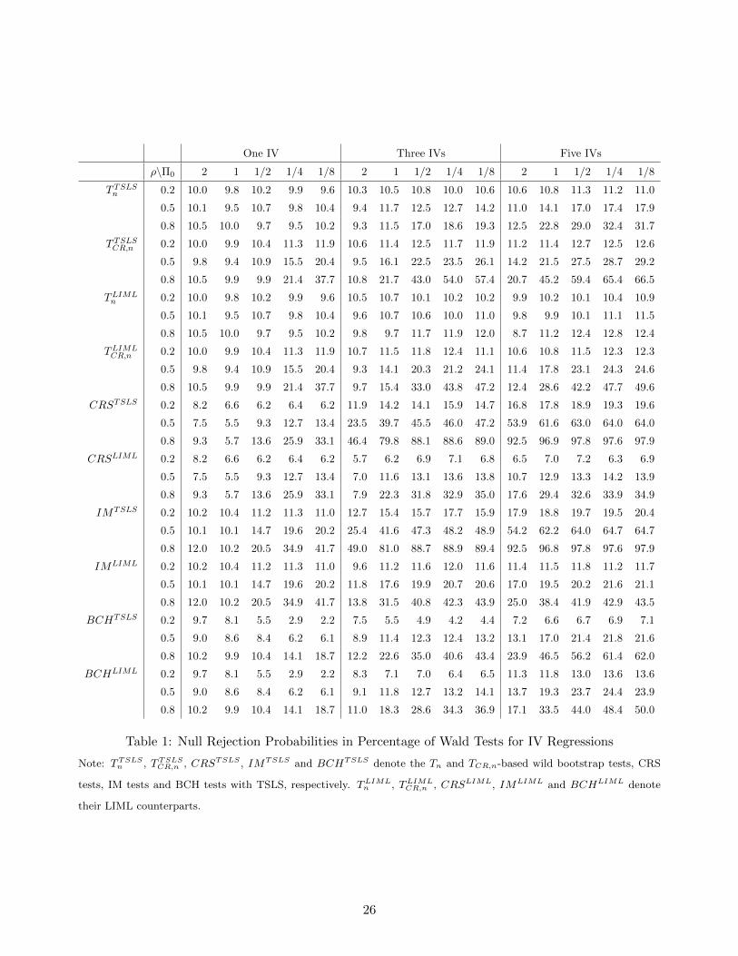
Table 1 reports the null empirical rejection frequencies of the Wald tests that are based
on TSLS and LIML, respectively, including the Tn and TCR,n-based wild bootstrap procedures
in Section 2.1, the randomization tests of CRS, the group-based t-tests of IM, and the CCE-
based t-tests with Bester et al. (2011, BCH)’s critical values. The TSLS and LIML-based tests
are numerically the same with one IV. We highlight several observations below. First, in line
with Remark 4, the Tn-based bootstrap tests have null rejection frequencies very close to the
nominal level with one IV. Except for this case, size distortions increase for all tests in Table
1 when the IVs become weak, the degree of endogeneity becomes high, or the number of IV
becomes large. Second, CRS and IM’s tests with LIML have substantial improvement upon their
counterparts with TSLS. This may be due to the fact that these tests are based on cluster-level
estimates, which could produce serious finite-sample bias when TSLS is employed, especially in
the over-identified case. All the other LIML-based procedures, including the bootstrap tests,
also have improvement upon their TSLS-based counterparts. Third, overall the wild bootstrap
procedures compare favorably with alternative approaches in terms of size control, and the
Tn-based procedure is found to have the smallest size distortions among these test procedures
no matter when TSLS or LIML is used. In particular, the bootstrap tests with LIML has null
rejection frequencies close to the nominal level across different settings of IV strength, degree
of endogeneity and number of IVs.
Table 2 reports the null rejection frequencies of AR tests, including the ARCR,n and ARR,n-
based asymptotic tests, which reject the null when the value of corresponding test statistic
exceeds χ2dz ,1−α, the 1− α quantile of the chi-squared distribution with dz degrees of freedom.
Additionally, it reports the rejection frequencies of the three wild bootstrap AR tests in Section
2.2 that are based on ARn, ARCR,n, and ARR,n, respectively. We notice that ARCR,n-based
asymptotic tests control the size but under-reject in the over-identified case.17 On the other
hand, the ARR,n-based asymptotic tests tend to have substantial over-rejections. By contrast,
the three bootstrap AR tests always have rejection frequencies very close to the nominal level.
Figure 1 compares the power properties of the tests that have good size control across
different settings, namely the Tn-based bootstrap tests, the three bootstrap AR tests and the
ARCR,n-based asymptotic AR tests. We also include TCR,n-based bootstrap tests for power
comparison with its Tn-based counterpart. We let the number of IVs equal to 3 and Π0 equal
17The null rejection probabilities of this AR test decrease toward zero when dz approaches q. When dz is equal
to q, the value of ARCR,n will be exactly equal to dz (or q), and thus has no variation (for f =(f1, ..., fq
)>and
fj = n−1∑i∈In,j
fi,j , ARCR,n = ι>q f(f>f
)−1
f>ιq = ι>q ιq = dz as long as f is invertible, where ιq denotes a q-
dimensional vector of ones). By contrast, the ARn-based bootstrap test works well even when dz is larger than q.
25
One IV Three IVs Five IVs
ρ\Π0 2 1 1/2 1/4 1/8 2 1 1/2 1/4 1/8 2 1 1/2 1/4 1/8
T TSLSn 0.2 10.0 9.8 10.2 9.9 9.6 10.3 10.5 10.8 10.0 10.6 10.6 10.8 11.3 11.2 11.0
0.5 10.1 9.5 10.7 9.8 10.4 9.4 11.7 12.5 12.7 14.2 11.0 14.1 17.0 17.4 17.9
0.8 10.5 10.0 9.7 9.5 10.2 9.3 11.5 17.0 18.6 19.3 12.5 22.8 29.0 32.4 31.7
T TSLSCR,n 0.2 10.0 9.9 10.4 11.3 11.9 10.6 11.4 12.5 11.7 11.9 11.2 11.4 12.7 12.5 12.6
0.5 9.8 9.4 10.9 15.5 20.4 9.5 16.1 22.5 23.5 26.1 14.2 21.5 27.5 28.7 29.2
0.8 10.5 9.9 9.9 21.4 37.7 10.8 21.7 43.0 54.0 57.4 20.7 45.2 59.4 65.4 66.5
TLIMLn 0.2 10.0 9.8 10.2 9.9 9.6 10.5 10.7 10.1 10.2 10.2 9.9 10.2 10.1 10.4 10.9
0.5 10.1 9.5 10.7 9.8 10.4 9.6 10.7 10.6 10.0 11.0 9.8 9.9 10.1 11.1 11.5
0.8 10.5 10.0 9.7 9.5 10.2 9.8 9.7 11.7 11.9 12.0 8.7 11.2 12.4 12.8 12.4
TLIMLCR,n 0.2 10.0 9.9 10.4 11.3 11.9 10.7 11.5 11.8 12.4 11.1 10.6 10.8 11.5 12.3 12.3
0.5 9.8 9.4 10.9 15.5 20.4 9.3 14.1 20.3 21.2 24.1 11.4 17.8 23.1 24.3 24.6
0.8 10.5 9.9 9.9 21.4 37.7 9.7 15.4 33.0 43.8 47.2 12.4 28.6 42.2 47.7 49.6
CRSTSLS 0.2 8.2 6.6 6.2 6.4 6.2 11.9 14.2 14.1 15.9 14.7 16.8 17.8 18.9 19.3 19.6
0.5 7.5 5.5 9.3 12.7 13.4 23.5 39.7 45.5 46.0 47.2 53.9 61.6 63.0 64.0 64.0
0.8 9.3 5.7 13.6 25.9 33.1 46.4 79.8 88.1 88.6 89.0 92.5 96.9 97.8 97.6 97.9
CRSLIML 0.2 8.2 6.6 6.2 6.4 6.2 5.7 6.2 6.9 7.1 6.8 6.5 7.0 7.2 6.3 6.9
0.5 7.5 5.5 9.3 12.7 13.4 7.0 11.6 13.1 13.6 13.8 10.7 12.9 13.3 14.2 13.9
0.8 9.3 5.7 13.6 25.9 33.1 7.9 22.3 31.8 32.9 35.0 17.6 29.4 32.6 33.9 34.9
IMTSLS 0.2 10.2 10.4 11.2 11.3 11.0 12.7 15.4 15.7 17.7 15.9 17.9 18.8 19.7 19.5 20.4
0.5 10.1 10.1 14.7 19.6 20.2 25.4 41.6 47.3 48.2 48.9 54.2 62.2 64.0 64.7 64.7
0.8 12.0 10.2 20.5 34.9 41.7 49.0 81.0 88.7 88.9 89.4 92.5 96.8 97.8 97.6 97.9
IMLIML 0.2 10.2 10.4 11.2 11.3 11.0 9.6 11.2 11.6 12.0 11.6 11.4 11.5 11.8 11.2 11.7
0.5 10.1 10.1 14.7 19.6 20.2 11.8 17.6 19.9 20.7 20.6 17.0 19.5 20.2 21.6 21.1
0.8 12.0 10.2 20.5 34.9 41.7 13.8 31.5 40.8 42.3 43.9 25.0 38.4 41.9 42.9 43.5
BCHTSLS 0.2 9.7 8.1 5.5 2.9 2.2 7.5 5.5 4.9 4.2 4.4 7.2 6.6 6.7 6.9 7.1
0.5 9.0 8.6 8.4 6.2 6.1 8.9 11.4 12.3 12.4 13.2 13.1 17.0 21.4 21.8 21.6
0.8 10.2 9.9 10.4 14.1 18.7 12.2 22.6 35.0 40.6 43.4 23.9 46.5 56.2 61.4 62.0
BCHLIML 0.2 9.7 8.1 5.5 2.9 2.2 8.3 7.1 7.0 6.4 6.5 11.3 11.8 13.0 13.6 13.6
0.5 9.0 8.6 8.4 6.2 6.1 9.1 11.8 12.7 13.2 14.1 13.7 19.3 23.7 24.4 23.9
0.8 10.2 9.9 10.4 14.1 18.7 11.0 18.3 28.6 34.3 36.9 17.1 33.5 44.0 48.4 50.0
Table 1: Null Rejection Probabilities in Percentage of Wald Tests for IV Regressions
Note: TTSLSn , TTSLSCR,n , CRSTSLS , IMTSLS and BCHTSLS denote the Tn and TCR,n-based wild bootstrap tests, CRS
tests, IM tests and BCH tests with TSLS, respectively. TLIMLn , TLIML
CR,n , CRSLIML, IMLIML and BCHLIML denote
their LIML counterparts.
26

One IV Three IVs Five IVs
ρ\Π0 2 1 1/2 1/4 1/8 2 1 1/2 1/4 1/8 2 1 1/2 1/4 1/8
ARn 0.2 10.1 9.8 10.2 10.0 9.7 10.8 10.4 10.3 9.9 10.3 10.7 10.2 9.4 10.0 10.2
0.5 10.1 9.6 10.7 9.8 10.4 9.9 11.4 10.4 9.9 10.4 10.5 9.2 9.5 9.9 10.4
0.8 10.5 10.0 9.8 9.6 10.3 11.0 10.7 11.1 9.8 10.2 9.9 10.4 10.2 10.5 10.4
ARCR,n 0.2 10.1 9.8 10.2 10.0 9.7 10.5 10.6 10.5 9.4 9.9 10.6 10.7 9.5 9.6 10.0
0.5 10.1 9.6 10.7 9.8 10.4 10.2 10.2 10.3 9.5 9.2 10.2 10.8 9.8 10.1 10.8
0.8 10.5 10.0 9.8 9.6 10.3 10.1 10.2 10.2 10.3 9.9 9.9 9.9 10.5 10.8 10.5
ARR,n 0.2 9.9 9.7 10.2 9.8 9.6 10.7 10.7 10.9 9.3 10.0 10.7 10.3 9.4 9.7 9.5
0.5 9.9 9.6 10.8 9.8 10.4 10.0 10.2 10.6 9.1 9.1 10.4 10.6 9.2 10.0 10.9
0.8 10.4 10.0 9.5 9.7 10.3 10.5 10.5 10.6 10.2 10.1 9.9 10.4 10.7 10.6 10.3
ARASYCR,n 0.2 9.2 9.3 9.7 9.6 9.5 5.1 5.1 5.4 4.2 4.7 0.8 0.6 0.5 0.6 0.6
0.5 9.1 9.1 10.4 9.4 10.0 5.3 4.9 5.3 4.7 4.3 0.6 0.8 0.6 0.5 0.6
0.8 10.3 9.5 9.3 9.3 9.7 5.0 5.0 5.1 5.5 5.0 0.5 0.6 0.5 0.7 0.6
ARASYR,n 0.2 15.8 15.1 15.5 15.5 15.1 32.0 31.8 32.1 30.7 31.2 56.0 55.3 54.5 54.7 55.5
0.5 15.0 15.1 16.6 15.6 16.5 32.2 32.3 30.7 30.6 30.4 54.6 55.1 53.9 54.6 56.5
0.8 16.2 16.2 15.2 15.4 15.9 32.5 32.4 31.5 30.9 31.0 55.9 55.1 54.6 56.6 55.0
Table 2: Null Rejection Probabilities in Percentage of AR Tests for IV Regressions
Note: ARn, ARCR,n and ARR,n denote the three wild bootstrap AR tests, and ARASYCR,n and ARASYR,n denote the ARCR,n
and ARR,n-based asymptotic AR tests with chi-squared critical values.
to 2 or 1.18 For the Wald tests, we use both LIML and its modified version proposed by Fuller
(1977, FULL), which has finite moments and is thus less dispersed than LIML.19 First, we
notice that among the AR tests, the ARn-based bootstrap tests have the highest power while
the asymptotic AR tests have the lowest, with the ARCR,n and ARR,n-based bootstrap tests
having almost the same power. Second, the Tn-based bootstrap tests with LIML have power
properties very similar to the ARn-based bootstrap tests. Third, the bootstrap tests with FULL
are always more powerful than their LIML counterparts. Fourth, in line with our theory, the
TCR,n-based bootstrap tests are more powerful than their Tn-based counterparts across different
settings, and therefore may be preferred when identification is strong.
5.2 IVQR
To examine the performance of wild bootstrap inference for the IVQR, we consider the fol-
lowing DGP. Let al,j = (al,1,j, · · · , al,n/q,j)> for l = 1, · · · , K, where K ≥ 1 is the number
of instruments, and vl,j = (vl,1,j, · · · , vl,n/q,j)> for l = 1, 2. Then, a1,j, · · · , aK,j, v1,j, v2,j are
independent across j ∈ J , each of them follow an n/q×1 multivariate normal distribution with
18Simulation results for other settings show similar patterns and are available upon request.19Following the recommendation in the literature, we set the tuning parameter of FULL equal to 1, in which case
FULL is best unbiased to second order among k-class estimators when the errors are normal (Rothenberg, 1984).
27

Figure 1: Power of Wild Bootstrap Wald and AR Tests for IV Regressions
Note: “boot.LIML.US”, “boot.LIML.CR”, “boot.FULL.US” and “boot.FULL.CR” denote the Tn and TCR,n-based wild
bootstrap tests with LIML and FULL, respectively. “asy.AR.CR” denote the ARCR,n-based AR tests with asymptotic
CVs, and “boot.AR.US”, “boot.AR.CR” and “boot.AR.R” denote the ARn, ARCR,n and ARR,n-based wild bootstrap
AR tests.
28

mean zero and covariance Σ(ρj), where Σ(ρj) is an n/q × n/q toeplitz matrix with coefficient
ρj and ρj = 0.2 + 0.05j. Define u1,i,j = v1,i,j, u2,i,j = ρv1,i,j +√
1− ρ2v2,i,j,
Yi,j = Xi,jβ +W i,jγ + (0.25 + 0.5W i,j + 0.1Xi,j)u1,i,j, Xi,j = 0.6√j +
K∑k=1
ΠkG(Zk,i,j) +G(u2,i,j),
Z1,i,j = a1,i,j, Zk,i,j = 0.6a1,i,j +√
0.64ak,i,j,∀k ≥ 2,
where Wi,j = (1,W i,j)>, W i,j is chi-square(1)
2distributed, and G(·) is the standard normal CDF.
We set β = 0.5, γ = 0, ρ = 0.5, Π1 = · · · = ΠK = Π0, Π0 ∈ (1, 1/2, 1/4, 1/8), n = 500, q = 10,
and the numbers of bootstrap and simulation replications to be 500, and test the following
hypothesis for K ∈ 1, 5 and τ ∈ 0.1, 0.25, 0.5, 0.75, 0.9:
H0 : β(τ) = 0.5 + 0.1G−1(τ) v.s. H1 : β(τ) = 1 + 0.1G−1(τ).
To implement the IVQR, we let the original IV be Φi,j(τ) = Φi,j(τ) = Zi,j and obtain Φi,j(τ)
as Φi,j(τ) = Φi,j(τ)− χ>j (τ)Wi,j, where Wi,j = (1,W i,j)> and χ(τ) is computed following (35).
Specifically, when computing TQRn and TQRCR,n, we first use Zi,j as IV, implement the IVQR, and
obtain the preliminary estimator (β(τ), γ(τ)). We then define the residual as
εi,j = yi,j −X>i,jβ(τ)−W>i,jγ(τ) (34)
When computing ARQRn and ARQR
CR,n, we let β(τ) be the value imposed under the null and
alternative and compute γ(τ) via a linear quantile regression of Yi,j −Xi,jβ(τ) on (Wi,j, Zi,j).
Given the estimator γ(τ), we define the residual as εi,j as (34). To compute χj(τ), we use the
fourth order Epanechnikov kernel and the rule of thumb bandwidth
h = 3.536s(q4τ − 6q2
τ + 3)−2/9n−1/5,
where qτ is the τth quantile of the standard normal distribution and s is the standard error of
εi,ji∈Ij ,j∈J .20
To compute TQRCR,n and ARQRn , we set the weighting matrix Aφ = Idφ , where Iφ is the φ× φ
identity matrix. To compute TQRn , we set Aφ(τ) = Iφ and Ar(τ) = 1. To compute the test
statistics TQRCR,n and AQRCR,n with the CCE, we use the same kernel and bandwidth as described
above to compute Ar,CR(τ) and ACR(τ) defined in (29) and Assumption 12(ii), respectively. For
comparison, we also compute the rejection probabilities for the randomization test of Canay
et al. (2017) and denote their test as CRS.
Table 3 collects the simulation results when the nominal rate of rejection is 10%.21 We can
make five observations. First, both ARQRn and ARQR
CR,n control size regardless of IV strength
20This is the optimal bandwidth that minimizes the MSE of the kernel density estimator at qτ when the underlying
density is Gaussian and the data are i.i.d.21The rejection probabilities using ARQRn and ARQRCR,n are numerically the same with one IV.
29
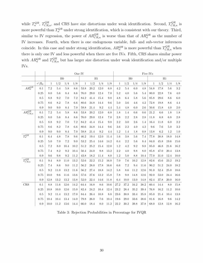
while TQRn , TQRCR,n, and CRS have size distortions under weak identification. Second, TQRCR,n is
more powerful than TQRn under strong identification, which is consistent with our theory. Third,
similar to IV regression, the power of ARQRCR,n is worse than that of ARQR
n as the number of
IV increases. Fourth, when there is one endogenous variable, full- and sub-vector inferences
coincide. In this case and under strong identification, ARQRn is more powerful than TQRCR,n when
there is only one IV and less powerful when there are five IVs. Fifth, CRS shares similar power
with ARQRn and TQRCR,n but has larger size distortion under weak identification and/or multiple
IVs.
One IV Five IVs
H0 H1 H0 H1
τ\Π0 1 1/2 1/4 1/8 1 1/2 1/4 1/8 1 1/2 1/4 1/8 1 1/2 1/4 1/8
ARQRn 0.1 7.2 5.4 5.8 8.6 53.8 20.2 12.0 6.8 4.2 5.4 6.0 4.8 54.8 17.8 5.6 3.2
0.25 8.0 5.6 8.4 8.6 76.0 29.0 12.4 7.0 5.2 4.0 5.6 5.4 80.0 22.8 7.6 4.0
0.5 8.8 9.2 7.0 7.2 84.2 41.4 15.4 9.8 4.8 6.4 5.8 5.6 85.8 29.6 8.6 6.0
0.75 8.6 8.2 7.8 6.6 80.6 34.8 14.4 9.6 5.0 3.6 4.6 4.2 72.8 19.8 8.6 4.4
0.9 9.0 9.0 8.4 7.0 59.8 21.4 9.2 4.4 5.4 4.8 6.0 2.6 50.6 15.8 4.0 2.0
ARQRCR,n 0.1 7.2 5.4 5.8 8.6 53.8 20.2 12.0 6.8 1.8 1.4 0.6 0.6 21.2 6.6 1.8 1.8
0.25 8.0 5.6 8.4 8.6 76.0 29.0 12.4 7.0 2.8 2.2 2.8 2.8 11.8 6.8 6.8 2.8
0.5 8.8 9.2 7.0 7.2 84.2 41.4 15.4 9.8 2.2 3.0 2.6 1.4 16.4 11.8 6.0 2.2
0.75 8.6 8.2 7.8 6.6 80.6 34.8 14.4 9.6 3.6 2.2 4.0 4.2 9.6 7.6 5.0 3.2
0.9 9.0 9.0 8.4 7.0 59.8 21.4 9.2 4.4 1.2 1.4 1.8 0.8 13.8 6.2 1.2 1.0
TQRn 0.1 6.4 4.8 7.8 9.6 46.2 19.4 12.0 11.4 1.6 3.8 5.6 7.4 77.8 38.8 18.0 14.8
0.25 5.0 7.0 7.2 9.0 53.2 25.4 14.6 14.2 0.4 2.2 5.6 8.4 84.0 45.8 19.6 15.6
0.5 7.2 8.0 10.4 10.2 51.2 25.2 15.4 12.0 1.2 4.2 9.2 9.8 85.0 46.8 21.6 16.2
0.75 7.4 8.2 9.2 10.4 50.4 24.0 9.8 13.2 2.2 4.0 9.8 8.0 85.8 47.0 20.4 13.8
0.9 9.6 9.8 9.2 11.2 43.8 18.2 11.4 8.0 1.2 5.0 8.8 10.4 77.0 31.0 12.4 10.0
TQRCR,n 0.1 9.4 8.0 11.0 13.2 52.6 22.2 15.2 16.0 7.0 7.6 10.2 12.8 82.6 45.6 23.2 19.2
0.25 7.4 8.6 9.0 11.2 56.2 28.0 17.8 16.6 6.6 7.2 9.4 11.6 90.2 51.2 24.0 18.2
0.5 9.2 11.0 13.2 11.6 56.2 27.4 18.8 14.2 5.8 8.6 11.2 12.6 91.0 52.4 25.0 18.6
0.75 10.0 9.6 11.6 13.6 57.6 27.6 12.2 15.8 7.8 9.8 14.8 12.6 92.0 53.0 24.4 16.6
0.9 12.8 13.2 13.2 13.8 52.0 22.4 14.6 11.8 6.4 10.0 13.0 14.8 82.4 37.8 20.0 16.0
CRS 0.1 8.8 11.6 12.6 14.2 64.4 16.8 8.6 10.6 27.2 37.2 34.2 38.2 60.4 14.4 8.0 15.8
0.25 10.8 10.0 12.6 15.0 82.4 24.2 10.4 12.4 23.2 28.4 35.2 39.4 76.8 16.2 11.2 10.6
0.5 9.2 11.4 13.2 17.0 84.4 26.4 10.8 8.8 23.6 30.8 33.4 35.8 85.0 21.4 10.4 13.8
0.75 10.4 10.4 13.4 14.0 79.8 26.0 7.6 10.4 19.6 29.0 33.6 38.6 81.6 16.8 9.6 14.2
0.9 10.0 11.2 13.6 14.4 66.0 18.4 8.0 11.2 22.2 30.2 39.8 37.8 68.0 12.8 12.8 16.2
Table 3: Rejection Probabilities in Percentage for IVQR
30

5.3 Practical Recommendations
For both linear IV and IV quantile regressions, we have the following practical recommenda-
tions. First, when conducting the full-vector inference, we suggest using the wild bootstrap AR
tests with deterministic studentization (i.e., ARn and ARQRn -based tests), which control size
irrespective of the strength of the IVs and have power advantage over the wild bootstrap AR
tests with CCE in the over-identified case. Second, to conduct the subvector inference that is
fully robust to weak IVs, one may apply the projection approach after the AR-based full-vector
inference. However, projection may result in power loss with multiple endogenous variables or
quantile indexes. Third, for conducting the subvector inference with at least one strong clus-
ter, we may implement the wild bootstrap Wald tests. In particular, those with deterministic
studentization (i.e., Tn and TQRn -based tests) have relative good size properties. On the other
hand, those with CCE (i.e., TCR,n and TQRCR,n-based tests) have better power properties, and is
therefore recommended when we are confident that the identification is strong. Fourth, in the
special case with only one endogenous regressor, the sub- and full-vector inferences coincide. In
this case, ARn and Tn are numerically the same for the linear IV regression. Therefore, under
strong identification, we recommend using TCR,n rather than ARn or Tn for better power. How-
ever, for IVQR, ARQRn and TQRn are not numerically the same. We recommend using ARQR
n
when there is only one IV and using TQRCR,n under strong identification and multiple IVs.
6 Empirical Application
In an influential study, Autor et al. (2013) analyze the effect of rising Chinese import compe-
tition on wages and employment in US local labor markets between 1990 and 2007, when the
share of total US spending on Chinese goods increased substantially from 0.6 percent to 4.6
percent. The dataset of Autor et al. (2013) includes 722 commuting zones (CZs) that cover
the entire mainland US. In this section, we further analyze the region-wise average and dis-
tributional effects of such import exposure by applying IV and IVQR with the proposed wild
bootstrap procedures to three Census Bureau-designated regions: South, Midwest and West,
with 16, 12 and 11 states, respectively, in each region.22
For both IV and IVQR models, we let the outcome variable (yi,j) denote the decadal change
in average individual log weekly wage in a given CZ. The endogenous variable (Xi,j) is the
change in Chinese import exposure per worker in a CZ, which is instrumented (Zi,j) by Chinese
import growth in other high-income countries.23 In addition, the exogenous variables (Wi,j)
include the characteristic variables of CZs and decade specified in Autor et al. (2013) as well
22The Northeast region is not included in the study due to the relatively small number of states (9) and small number
of CZs in each states (e.g., Connecticut and Rhode Island only have 2 CZs, respectively).23See Sections I.B and III.A in Autor et al. (2013) for detailed definition of these variables.
31

as state fixed effects. Our regressions are based on the CZ samples in each region, and the
samples are clustered at state level, following Autor et al. (2013). Besides the results for the
full sample, we also report those for female and male samples separately.
The main result of the IV regression for the three regions is given in Table 4, with the
numbers of observations (n, the number of CZs in each region) and clusters (q, the number
of states in each region), the TSLS estimates, and the 90% bootstrap confidence sets (CSs)
constructed by inverting the corresponding Tn-based (equivalently, ARn-based) wild bootstrap
tests with 10% nominal level. The computation of the bootstrap CSs was conducted over the
parameter space [−10, 10] with a step size of 0.01, and the number of bootstrap draws is set at
2,000 for each step. The results in Table 4 suggest that there may exist regional heterogeneity
in terms of the average effect of Chinese import on wages in local labor markets. For instance,
the TSLS estimates for South and West regions equal −0.97 and −1.05, respectively, while
that for Midwest region equals −0.025, i.e., a $1, 000 per worker increase in a CZ’s exposure
to Chinese imports is estimated to reduce average weekly earnings by 0.97, 1.05 and 0.025 log
points, respectively, for the three regions (the corresponding TSLS estimate in Autor et al.
(2013) for the entire mainland US is −0.76). Furthermore, according to the wild bootstrap
procedure, the effect on CZs in South is significantly different from zero at the 10% level, while
those on CZs in the other two regions are not. Compared with that for South, the wider CSs
for Midwest and West may be due to relatively weak identification, which our procedure is able
to guard against. Table 4 also reports the results for female and male samples. We find that
across all the regions, the effects are more substantial for the male samples. Moreover, the
effects for both female and male samples in South are significantly different from zero.
All Female Male
Region n q Estimate Bootstrap CS Estimate Bootstrap CS Estimate Bootstrap CS
South 578 16 -0.97 [-1.73, -0.58] -0.81 [-1.49, -0.40] -1.08 [-1.95, -0.66]
Midwest 504 12 -0.025 [-0.68,0.78] 0.024 [-0.63,0.74] -0.17 [-1.04,0.77]
West 276 11 -1.05 [-1.47,0.26] -0.6 [-1.49,0.82] -1.26 [-1.99,0.73]
Table 4: IV regressions of Autor et al. (2013) with all, female, and male samples for three US regions
Next, we study the region-wise distributional effects of Chinese import competition by run-
ning IVQR for South, Midwest and West regions separately, and the results are reported in
Table 5. The IVQR point estimates are computed using the original IV (Chinese import
growth in other high-income countries) without any projection on the exogenous variables.
The weak-IV-robust 90% bootstrap CSs are computed by inverting the ARQRn test when the
IV is computed via the projection described in Remark 12 with εi,j(τ) constructed via (23) so
that the null hypothesis is imposed. For the results of Midwest and West regions, some CSs
32

contain several segments as the identification can be rather weak. We follow Chernozhukov and
Hansen (2008) and use the maximum and minimum values admitted by the ARQRn test as the
two endpoints of our CSs. The resulting interval covers all the segments, and thus, controls
coverage asymptotically. We provide the bootstrap p-values of the ARQRn tests for all our IVQR
results in Section B in the Online Supplement. In line with the results in IV regressions, the
distributional effects of Chinese import competition are significantly negative for South region
at all quantiles except 90%, while those for Midwest and West regions are not significant at any
of the quantiles. Furthermore, similar to IV regressions, Table 5 shows that the negative effects
of import exposure are more substantial for the male samples at most quantiles. In addition,
the bootstrap CSs report that the effects are significant for male in South at the 10%, 50% and
75% quantiles, while significant for female at the 75% and 90% quantiles.
Last, for the South region, whose coefficients are strongly identified, we further test the
distributional homogeneity of the effect of Chinese import exposure on wage by considering the
following three null hypothesis:
H0 : β(0.1) = β(0.5), H0 : β(0.1) = β(0.9), and H0 : β(0.5) = β(0.9),
where β(τ) is the coefficient of interest and τ ∈ (0, 1) is the quantile index. We conduct
the Wald-test based subvector inference for IVQR that involves two quantile indexes.24 The
bootstrap p-values for the three hypotheses are reported in Table 6 below. We can make three
observations. First, the p-values computed based on the Wald test with CCE (i.e., TQRCR,n) are all
smaller than those without. This is consistent with our theory that TQRCR,n is more powerful than
TQR in detecting more distant alternatives when there is only one restriction. Second, we reject
the null hypothesis of β(0.1) = β(0.9) for female and male samples at 1% and 5% significance
levels, respectively. Third, although we cannot reject β(0.1) = β(0.9) for the full sample, this
does not contradict with the previous significant results because it is not a combination of the
female and male samples. In fact, the samples are obtained by averaging data in a given CZ for
all, female, and male individuals, respectively, and they therefore share the same sample size.
24We refer readers to Section Q in the Online Supplement for its implementation detail and theoretical guarantee.
33
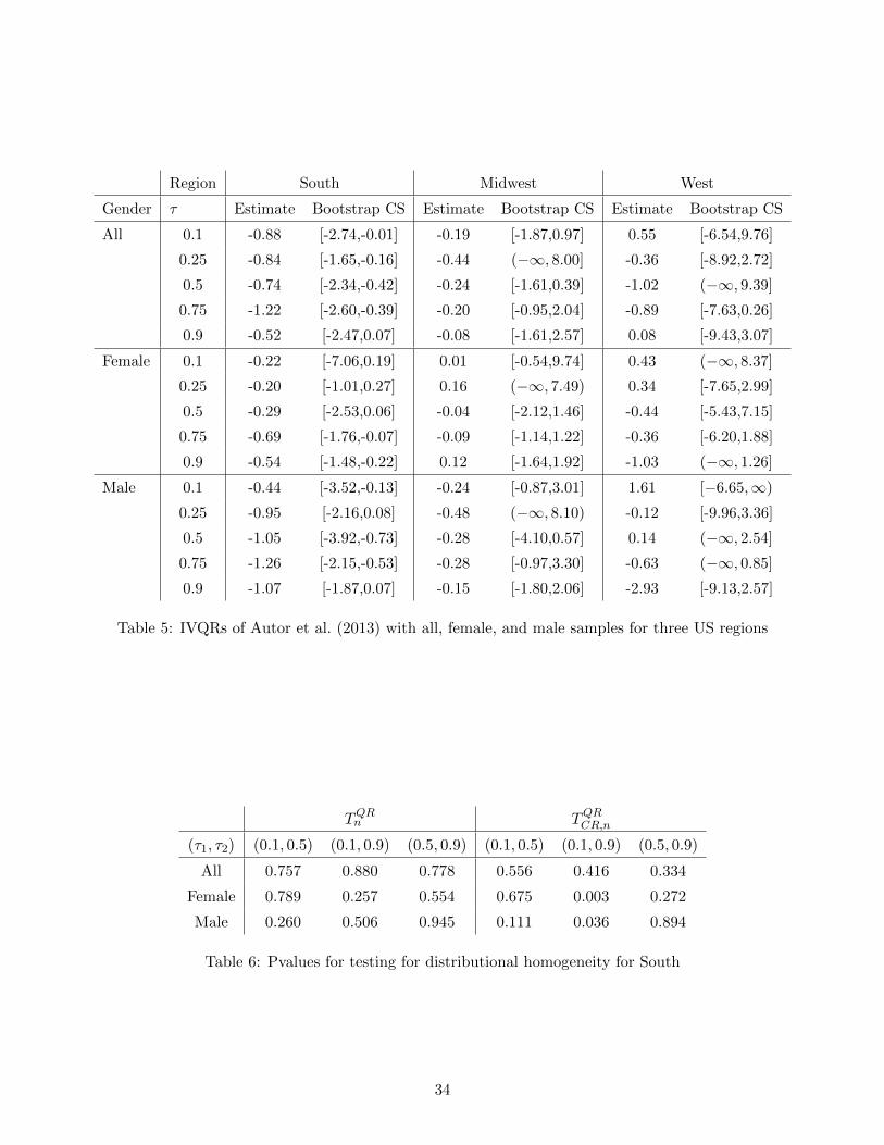
Region South Midwest West
Gender τ Estimate Bootstrap CS Estimate Bootstrap CS Estimate Bootstrap CS
All 0.1 -0.88 [-2.74,-0.01] -0.19 [-1.87,0.97] 0.55 [-6.54,9.76]
0.25 -0.84 [-1.65,-0.16] -0.44 (−∞, 8.00] -0.36 [-8.92,2.72]
0.5 -0.74 [-2.34,-0.42] -0.24 [-1.61,0.39] -1.02 (−∞, 9.39]
0.75 -1.22 [-2.60,-0.39] -0.20 [-0.95,2.04] -0.89 [-7.63,0.26]
0.9 -0.52 [-2.47,0.07] -0.08 [-1.61,2.57] 0.08 [-9.43,3.07]
Female 0.1 -0.22 [-7.06,0.19] 0.01 [-0.54,9.74] 0.43 (−∞, 8.37]
0.25 -0.20 [-1.01,0.27] 0.16 (−∞, 7.49) 0.34 [-7.65,2.99]
0.5 -0.29 [-2.53,0.06] -0.04 [-2.12,1.46] -0.44 [-5.43,7.15]
0.75 -0.69 [-1.76,-0.07] -0.09 [-1.14,1.22] -0.36 [-6.20,1.88]
0.9 -0.54 [-1.48,-0.22] 0.12 [-1.64,1.92] -1.03 (−∞, 1.26]
Male 0.1 -0.44 [-3.52,-0.13] -0.24 [-0.87,3.01] 1.61 [−6.65,∞)
0.25 -0.95 [-2.16,0.08] -0.48 (−∞, 8.10) -0.12 [-9.96,3.36]
0.5 -1.05 [-3.92,-0.73] -0.28 [-4.10,0.57] 0.14 (−∞, 2.54]
0.75 -1.26 [-2.15,-0.53] -0.28 [-0.97,3.30] -0.63 (−∞, 0.85]
0.9 -1.07 [-1.87,0.07] -0.15 [-1.80,2.06] -2.93 [-9.13,2.57]
Table 5: IVQRs of Autor et al. (2013) with all, female, and male samples for three US regions
TQRn TQRCR,n
(τ1, τ2) (0.1, 0.5) (0.1, 0.9) (0.5, 0.9) (0.1, 0.5) (0.1, 0.9) (0.5, 0.9)
All 0.757 0.880 0.778 0.556 0.416 0.334
Female 0.789 0.257 0.554 0.675 0.003 0.272
Male 0.260 0.506 0.945 0.111 0.036 0.894
Table 6: Pvalues for testing for distributional homogeneity for South
34

A Constructing the IVs
In this section, we discuss how to do projection at the cluster level for both IV regression and
IVQR even when the covariate W contains the cluster-level variables.
A.1 IV Regression
Suppose Zi,j is the original IV. We can construct Zi,j as Zi,j = Zi,j − χ>j Wi,j, where χj =
QWW,jQ−WW,jQ
−WW,jQWZ,j, QWW,j = 1
nj
∑i∈In,j Wi,jW
>i,j, QWW,j = 1
nj
∑i∈In,j Wi,jZ
>i,j, and A−
denotes the pseudo inverse of the positive semidefinite matrixA. We can show that 1nj
∑i∈In,j Zi,jW
>i,j =
0 following the same argument in the next section.
A.2 IVQR
A.2.1 Full-Sample Projection
We first consider the full-sample projection mentioned in the main paper.
Assumption 13. Define
Jγ,γ,j(τ) = limn→∞
Pn,jfεi,j(τ)(0|Wi,j, Zi,j)V2i,j(τ)Wi,jW
>i,j,
Jγ,θ,j
(τ) = limn→∞
Pn,jfεi,j(τ)(0|Wi,j, Zi,j)V2i,j(τ)Wi,jΦ
>i,j(τ),
Jγ,γ(τ) =∑j∈J
ξjJγ,γ,j(τ), Jγ,θ
(τ) =∑j∈J
ξjJ γ,θ,j(τ), and χ(τ) = J −1
γ,γ (τ)Jγ,θ
(τ).
(i) Suppose
supτ∈Υ
[||Jγ,γ,j(τ)− Jγ,γ,j(τ)||op + ||J
γ,θ,j(τ)− J
γ,θ,j(τ)||op
]= op(1).
(ii) Recall δi,j(v, τ) = X>i,jvb +W>i,jvr + Φ>i,j(τ)vt. Then,
sup∥∥∥Pn,jfεi,j(τ)(δi,j(v, τ)|Wi,j, Zi,j)V
2i,j(τ)Wi,jΦ
>i,j(τ)− J
γ,θ,j(τ)∥∥∥op
p−→ 0,
where the suprema are taken over j ∈ J, ||v||2 ≤ δ, τ ∈ Υ, v = (v>b , v>r , v
>t )>.
(iii) For j ∈ J , there exists χn,j(τ) such that
Jγ,θ,j
(τ) = Jγ,γ,j
(τ)χn,j(τ) and Pn,j||W>i,j(χ(τ)− χn,j(τ))||2op = o(1).
(iv) There exist constants c, C such that
0 < c < infτ∈Υ
λmin(Jγ,γ(τ)) ≤ supτ∈Υ
λmax(Jγ,γ(τ)) ≤ C <∞.
35

First, for subvector inference, we require the original IVs Φi,j(τ) to be valid, i.e., Assumptions
5, 6, 8(i)–8(iii) hold with Φi,j(τ) and Φi,j(τ) replaced by Φi,j(τ) and Φi,j(τ). Then, we construct
εi,j(τ) as
εi,j(τ) = Yi,j −X>i,jβ(τ)−W>i,j γ(τ),
where (β(τ), γ(τ)) are the IVQR estimator obtained via (19) and (20) with Φi,j(τ) replaced by
Φi,j(τ). Note that following the same argument as in Lemma L.1, we can show
supτ∈Υ
(||β(τ)− βn(τ)||2 + ||γ(τ)− γn(τ)||2
)= Op(n
−1/2).
For the full-vector inference, the IVs may be weak or invalid. Instead, we define εi,j(τ) as
εi,j(τ) = Yi,j −X>i,jβ0(τ)−W>i,j γ(β0(τ), τ),
where γ(β0(τ), τ) is the defined in (19) and β0(τ) is the null hypothesis. Then, under the null, we
have supτ∈Υ ||γ(β0(τ), τ)− γn(τ)||2 = Op(n−1/2). In both cases, εi,j(τ) is a valid approximation
of εi,j(τ) and Assumption 13(i) holds under mild regularity conditions. Second, Assumption
13 requires the nonparametric estimation of Jγ,γ,j(τ) and Jγ,θ,j
(τ) via kernel smoothing. We
discuss the choice of kernel function and bandwidth in Section 5. Third, Assumption 13(ii) holds
under mild smoothness conditions. Fourth, Assumption 13(iii) parallels Assumption 2(iv) so
that the same comments still apply.
Proposition A.1. Suppose Assumption 13 holds and Φi,j(τ) = Φi,j(τ)− χ>(τ)Wi,j where χ(τ)
is defined in (35). Then, Jγ,θ,j(τ) defined in Assumption 7 is zero for j ∈ J and τ ∈ Υ, i.e.,
by letting n→∞ followed by δ → 0, we have
sup∥∥∥Pn,jfεi,j(τ)(δi,j(v, τ)|Wi,j, Zi,j)V
2i,j(τ)Wi,jΦ
>i,j(τ)
∥∥∥op
p−→ 0,
where the suprema are taken over j ∈ J, ||v||2 ≤ δ, τ ∈ Υ for v = (v>b , v>r , v
>t )>.
A.2.2 Cluster-Level Projection
Suppose Φi,j(τ) and Φi,j(τ) are the original (infeasible) IV and its estimator, respectively, such
that Assumption 7(i) is violated, i.e.,
lim supn→∞
Pn,jfεi,j(τ)(0|Wi,j, Zi,j)Wi,j(τ)Φ>i,j(τ) 6= 0.
We construct Φi,j(τ) as Φi,j(τ) = Φi,j(τ) − χ>j (τ)Wi,j such that Assumption 7(i) holds with
Φi,j(τ) as the instrument. Let
χj(τ) = Jγ,γ,j(τ)J −γ,γ,j(τ)J −γ,γ,j(τ)Jγ,θ,j
(τ) (35)
36

where Jγ,γ,j(τ) and Jγ,θ,j
(τ) are defined in Section 3.25
Assumption 14. (i) Suppose
supτ∈Υ
[||Jγ,γ,j(τ)− Jγ,γ,j(τ)||op + ||Jγ,θ,j(τ)− J
γ,θ,j(τ)||op
]= op(1).
(ii) Recall δi,j(v, τ) = X>i,jvb +W>i,jvr + Φ>i,j(τ)vt. Then,
sup∥∥∥Pn,jfεi,j(τ)(δi,j(v, τ)|Wi,j, Zi,j)V
2i,j(τ)Wi,jΦ
>i,j(τ)− J
γ,θ,j(τ)∥∥∥op
p−→ 0,
where the suprema are taken over j ∈ J, ||v||2 ≤ δ, τ ∈ Υ, v = (v>b , v>r , v
>t )>.
(iii) Define the kth largest singular value of Jγ,γ,j(τ) as σk(Jγ,γ,j(τ)) for k ∈ [dw]. Then there
exist constants c, C and integer R ∈ [1, dw] such that
0 < c ≤ infτ∈Υ
σR(Jγ,γ,j(τ)) ≤ supτ∈Υ
σ1(Jγ,γ,j(τ)) ≤ C <∞.
The use of generalized inverse in (35) accommodates the case that Jγ,γ,j(τ) is not invertible.
Assumption 13(iii) only requires that the minimum nonzero eigenvalue of Jγ,γ,j(τ) is bounded
away from zero uniformly over τ ∈ Υ.
Proposition A.2. Suppose Assumption13 holds and Φi,j(τ) = Φi,j(τ)− χ>j (τ)Wi,j where χ>j (τ)
is defined in (35). Then, Jγ,θ,j(τ) defined in Assumption 7 is zero for j ∈ J and τ ∈ Υ, i.e.,
by letting n→∞ followed by δ → 0, we have
sup∥∥∥Pn,jfεi,j(τ)(δi,j(v, τ)|Wi,j, Zi,j)V
2i,j(τ)Wi,jΦ
>i,j(τ)
∥∥∥op
p−→ 0,
where the suprema are taken over j ∈ J, ||v||2 ≤ δ, τ ∈ Υ for v = (v>b , v>r , v
>t )>.
B Additional Empirical Results
In this section, we report the pvalues of the ARQRn tests with all, female, and male samples for
midwest, west, and south regions. In Figures 2–10, the X-axis represents the value of effect of
Chinese import on wage under the null while the Y-axis represents the corresponding pvalue.
C Proof of Theorems 2.1
The arguments follow those in Canay et al. (2020). Let S ≡ Rdz×dx×Rdz×dz×⊗j∈JRdz×Rdr×dr
and write an element s ∈ S by s = (s1, s2, s3,j : j ∈ J, s4) where s3,j ∈ Rdz for any j ∈ J .
25For a symmetric and positive semidefinite matrix A, we define A− as its generalized inverse. The expression for
χj(τ) is inspired by the minimum norm least squares solution of the normal equation that 1n
∑ni=1Xi(Yi − X
>i b) = 0
when 1n
∑ni=1XiX
>i is not invertible.
37
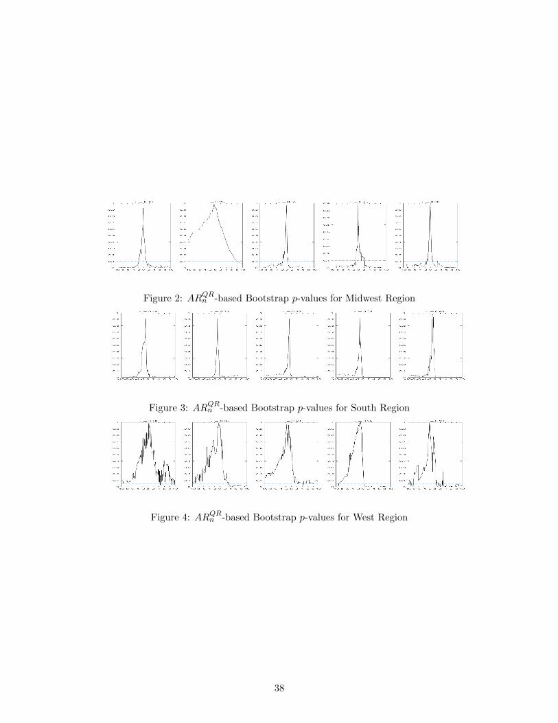
Figure 2: ARQRn -based Bootstrap p-values for Midwest Region
Figure 3: ARQRn -based Bootstrap p-values for South Region
Figure 4: ARQRn -based Bootstrap p-values for West Region
38

Figure 5: ARQRn -based Bootstrap p-values for the Female Sample in Midwest Region
Figure 6: ARQRn Pvalues for the Male Sample in Midwest Region
Figure 7: ARQRn Pvalues for the Female Sample in South Region
Figure 8: ARQRn Pvalues for the Male Sample in South Region
Figure 9: ARQRn Pvalues for the Female Sample in West Region
Figure 10: ARQRn Pvalues for the Female Sample in West Region
39

Define the function T : S→ R to be given by
T (s) =
∥∥∥∥λ>β (s′1s−12 s1
)−1s′1s−12
(∑j∈J
s3,j
)∥∥∥∥s4
(36)
for any s ∈ S such that s2 and s′1s−12 s1 are invertible and let T (s) = 0 otherwise. We
also identify any (g1, ..., gq) = g ∈ G = −1, 1q with an action on s ∈ S given by gs =
(s1, s2, gjs3,j : j ∈ J, s4). For any s ∈ S and G’ ⊆ G, denote the ordered values of T uw(gs) :
g ∈ G’ by T (1)(s|G’) ≤ . . . ≤ T (|G’|)(s|G’). Given this notation we can define the statistics
Sn, Sn ∈ S as
Sn =
QZX , QZZ ,
√nj√n
1√nj
∑i∈In,j
Zi,jεi,j : j ∈ J
, Ar
,
Sn =
QZX , QZZ ,
√nj√n
1√nj
∑i∈In,j
Zi,j εri,j : j ∈ J
, Ar
. (37)
Let En denote the event En = IQZX is of full rank value and QZZ is invertible
, and As-
sumption 1 implies that lim infn→∞ PEn = 1 = 1.
Note that whenever En = 1 and H0 is true, the Frisch-Waugh-Lovell theorem implies that
Tn =
∥∥∥∥√n(λ>β β − λ0
)∥∥∥∥Ar
=
∥∥∥∥√nλ>β (β − βn)∥∥∥∥Ar
=
∥∥∥∥λ>β Q−1Q>ZXQ−1
ZZ
∑j∈J
1√n
∑i∈In,j
Zi,jεi,j
∥∥∥∥Ar
= T (Sn). (38)
Similarly, we have for any action g ∈ G that
T ∗n(g) =
∥∥∥∥√nλ>β (β∗g − βr)∥∥∥∥Ar
=
∥∥∥∥λ>β Q−1Q′ZXQ−1
ZZ
∑j∈J
1√n
∑i∈In,j
gjZi,j εri,j
∥∥∥∥Ar
= T (gSn).(39)
Therefore, for any x ∈ R letting dxe denote the smallest integer larger than x and k∗ ≡d|G|(1− α)e, we obtain from (38)-(39) that
I Tn > cn(1− α) = IT (Sn) > T (k∗)(Sn|G)
. (40)
Furthermore, let ιq ∈ G correspond to the identity action, i.e., ιq = (1, ..., 1) ∈ Rq, and
similarly define −ιq = (−1, ...,−1) ∈ Rq. Since T (−ιqSn) = T (ιqSn), we obtain from (39) that
T(−ιqSn
)= T
(ιqSn
)=
∥∥∥∥λ>β Q−1Q>ZXQ−1
ZZ
∑j∈J
1√n
∑i∈In,j
Zi,j
(yi,j −X>i,jβr −W>
i,j γr)∥∥∥∥
Ar
=
∥∥∥∥λ>β Q−1Q>ZXQ−1
ZZ
∑j∈J
1√n
∑i∈In,j
Zi,j
(yi,j −X>i,jβr
)∥∥∥∥Ar
=∥∥√nλ>β (β − βr)
∥∥Ar
= T (Sn) , (41)
40

where the third equality follows from∑
j∈J∑
i∈In,j Zi,jW>i,j = 0. (41) implies that if k∗ ≡
d|G|(1− α)e > |G| − 2, then IT (Sn) > T (k∗)(Sn|G) = 0, and this gives the upper bound in
Theorem 2.1. We therefore assume that k∗ ≡ d|G|(1− α)e ≤ |G| − 2, in which case
lim supn→∞
PT (Sn) > T (k∗)(Sn|G);En = 1 = lim supn→∞
PT (Sn) > T (k∗)(Sn|G \ ±ιq);En = 1
≤ lim supn→∞
PT (Sn) ≥ T (k∗)(Sn|G \ ±ιq);En = 1,
(42)
where the first equality follows from (40), the second equality from (41) and k∗ ≤ |G| − 2, and
the final inequality follows by set inclusion.
Then, to examine the right hand side of (42), first note that by Assumptions 1-2 and the
continuous mapping theorem we haveQZX , QZZ ,
√nj√n
1√nj
∑i∈In,j
Zi,jεi,j : j ∈ J
, Ar
d−−→(QZX , QZZ ,
√ξjZj : j ∈ J
, A)≡ S,
(43)
where ξj > 0 for all j ∈ J by Assumption 2(ii), and QZZ denotes the limit of QZZ . We further
note that whenever En = 1, for every g ∈ G,∣∣∣T (gSn)− T (gSn)∣∣∣ ≤ ∥∥∥∥λ>β Q−1Q>
ZXQ−1
ZZ
∑j∈J
njn
1
nj
∑i∈In,j
gjZi,jX>i,j
√n(βn − βr)
∥∥∥∥Ar
+
∥∥∥∥λ>β Q−1Q>ZXQ−1
ZZ
∑j∈J
njn
1
nj
∑i∈In,j
gjZi,jW>i,j
√n(γ − γr)
∥∥∥∥Ar
. (44)
Note that whenever λ>β βn = λ0 it follows from Assumption 1 and Amemiya (1985, Eq.(1.4.5))
that√n(βr−βn) and
√n(γr−γ) are bounded in probability. Also, we have
∑i∈In,j Zi,jW
>i,j/nj =
op(1) by the same argument as in Lemma A.2 of Canay et al. (2020). Therefore,
lim supn→∞
P
∥∥∥∥λ>β Q−1Q>
ZXQ−1
ZZ
∑j∈J
njn
1
nj
∑i∈In,j
gjZi,jW>i,j
√n(γ − γr)
∥∥∥∥Ar
> ε;En = 1
= 0.
(45)
Under Assumption 3(i), λβ = 1 and βn = βr, so that we immediately have for any ε > 0,
lim supn→∞
P
∥∥∥∥λ>β Q−1Q>
ZXQ−1
ZZ
∑j∈J
njn
1
nj
∑i∈In,j
gjZi,jX>i,j
√n(βn − βr)
∥∥∥∥Ar
> ε;En = 1
= 0. (46)
41

Moreover, Assumption 3(ii) yields for any ε > 0 that
lim supn→∞
P
∥∥∥∥λ>β Q−1Q>
ZXQ−1
ZZ
∑j∈J
njn
1
nj
∑i∈In,j
gjZi,jX>i,j
√n(βn − βr)
∥∥∥∥Ar
> ε;En = 1
= lim sup
n→∞P
∥∥∥∥λ>β (Q>ZXQ−1
ZZQZX
)−1
Q>ZXQ−1
ZZ
∑j∈Js
ξjgjajQZX
√n(βn − βr)
∥∥∥∥Ar
> ε;En = 1
= lim supn→∞
P
∥∥∥∥∑j∈Js
ξjgjaj√n(λ>β β − λ>β βr)
∥∥∥∥Ar
> ε;En = 1
= 0, (47)
where the last equality holds because λ>β βr = λ0 under H0.
Note that T (gSn) = T (gSn) whenever En = 0 as we have defined T (s) = 0 for any s =
(s1, s2, s3,j : j ∈ J, s4) whenever s2 or s′1s−12 s1 is not invertible. Therefore, results in (44),
(45) and (47) imply that T (gSn) = T (gSn) + oP (1) for any g ∈ G, and we obtain from (43):(T (Sn),
T (gSn) : g ∈ G
)d−−→ (T (S), T (gS) : g ∈ G) . (48)
Moreover, since lim infn→∞ PEn = 1 = 1, it follows that(T (Sn), En, T (gSn) : g ∈ G
)converge jointly as well. Hence, Portmanteau’s theorem implies that
lim supn→∞
PT (Sn) ≥ T (k∗)(Sn|G \±ιq);En = 1
≤ PT (S) ≥ T (k∗)(S|G \±ιq) = PT (S) > T (k∗)(S|G \±ιq), (49)
where the equality follows from PT (S) = T (gS) = 0 for all g ∈ G\±ιq since the covariance
matrix of Zj is full rank for all j ∈ J , and the limit of Q−1Q>ZXQ−1
ZZis of full rank by Assumption
1. Finally, since T (ιqS) = T (−ιqS), we obtain that T (S) > T (k∗)(S|G \ ±ιq) if and only if
T (S) > T (k∗)(S|G), which yields
PT (S) > T (k∗)(S|G \±ιq) = PT (S) > T (k∗)(S|G) ≤ α, (50)
where the final inequality follows by gSd= S for all g ∈ G and the properties of randomization
tests. This completes the proof of the upper bound in the statement of the Theorem.
For the lower bound, first note that k∗ ≡ d|G|(1− α)e > |G| − 2 implies that α− 12q−1 ≤ 0,
in which case the result trivially follows. Now assume k∗ ≡ d|G|(1− α)e ≤ |G| − 2, then
lim supn→∞
PT (Sn) > T (k∗)(Sn|G) ≥ lim infn→∞
PT (Sn) > T (k∗)(Sn|G) ≥ PT (S) > T (k∗)(S|G)
≥ PT (S) > T (k∗+2)(S|G)+ PT (S) = T (k∗+2)(S|G) ≥ α− 1
2q−1,
(51)
where the first inequality follows from (40), the second inequality follows from Portmanteau’s
theorem, the third inequality holds because PT (z+2)(S|G) > T (z)(S|G) = 1 for any integer
42

z ≤ |G| − 2 by (36) and Assumption 2(i)-(ii), and the last equality follows from noticing that
k∗ + 2 = d|G|((1 − α) + 2/|G|)e = d|G|(1 − α′)e with α′ = α − 12q−1 and the properties of
randomization tests. This completes the proof of the lower bound.
For the power of the Tn-based wild bootstrap test, notice that
||√n(λ>β β − λ0)||Ar =||
√nλ>β (β − βn) +
√nλ>β (βn − βr)||Ar
=∥∥∥λ>β Q−1Q>
ZXQ−1
ZZ
∑j∈J
∑i∈In,j
Zi,jεi,j√n
+√nλ>β (βn − βr)
∥∥∥Ar
=∥∥∥λ>β Q−1Q>
ZXQ−1
ZZ
∑j∈J
∑i∈In,j
(Zi,jεi,j√
n+Zi,jX
>i,j
n
√n(βn − βr)
)∥∥∥Ar. (52)
Similarly, by Assumption 2(iv), we have for its bootstrap analogue,
||√nλ>β (β∗g − βr)||Ar
=∥∥∥λ>β Q−1Q>
ZXQ−1
ZZ
∑j∈J
∑i∈In,j
gj
(Zi,jεi,j√
n+Zi,jX
>i,j
n
√n(βn − βr) +
Zi,jW>i,j
n
√n(γn − γr)
)∥∥∥Ar
=∥∥∥λ>β Q−1Q>
ZXQ−1
ZZ
∑j∈J
∑i∈In,j
gj
(Zi,jεi,j√
n+Zi,jX
>i,j
n
√n(βn − βr)
)∥∥∥Ar
+ oP (1). (53)
Furthermore, we notice that
βr =β − Q−1λβ
(λ>β Q
−1λβ
)−1 (λ>β β − λ0
)=β − Q−1λβ
(λ>β Q
−1λβ
)−1
λ>β (β − βn) +(λ>β Q
−1λβ
)−1
(λ>β βn − λ0)
. (54)
Therefore, employing (54) with√n(λ>β βn − λ0) = λ>β µβ, we conclude that whenever En = 1,
∑i∈In,j
Zi,jX>i,j
n
√n(βn − βr) =
∑i∈In,j
Zi,jX>i,j
n
(Idx − Q−1λβ
(λ>β Q
−1λβ
)−1
λ>β
)√n(β − βn)
+Q−1λβ
(λ>β Q
−1λβ
)−1
λ>β µβ
. (55)
Together with (53), this implies that
lim supn→∞
Pµβ ,n
∥∥∥√nλ>β (β∗g − βr)− λ>β Q−1Q>
ZXQ−1
ZZ
×∑
j∈J∑
i∈In,j gj
(Zi,jεi,j√
n+ ξjQZX,jQ
−1λβ
(λ>β Q
−1λβ
)−1
λ>β µβ
)∥∥∥Ar> ε;En = 1
= lim sup
n→∞Pµβ ,n
∥∥∥√nλ>β (β∗g − βr)− λ>βQ−1Q>
ZXQ−1
ZZ
×∑
j∈J gj
[√ξjZj + ξjajQZXQ
−1λβ(λ>βQ
−1λβ)−1
µ] ∥∥∥
Ar> ε;En = 1
= 0.
The result then follows by applying the same arguments as those in the proof of Theorem 3.2
43

in Canay et al. (2020).
D Proof of Theorem 2.2
The proof for the asymptotic size of the TCR,n-based wild bootstrap test follows similar argu-
ments as those for the Tn-based wild bootstrap test and the arguments in the proof of Theorem
3.3 in Canay et al. (2020), and is thus omitted.
For the power analysis, we define
TCR,∞ =
∥∥∥∥∥λ>β Ω
[∑j∈J
gj√ξjZj
]+ µ
∥∥∥∥∥Ar,CR,ιg
,
where Ω = Q−1Q>ZXQ−1
ZZand
Ar,CR,ιg =
(∑j∈J ξj
λ>β Ω
[gjZj − aj
√ξj∑
j∈J√ξ jgjZj
]λ>β Ω
[gjZj − aj
√ξj∑
j∈J√ξ jgjZj
]>)−1
.
By the Portmanteau theorem, we have
lim infn→∞
P(TCR,n > cn) ≥ P(TCR,∞(ιq) > (TCR,∞)(k∗)
).
In addition, we aim to show that, as ||µ||2 →∞, we have
P(TCR,∞(ιq) > max
g∈Gs
TCR,∞(g)
)→ 1. (56)
Then, given |Gs| = |G| − 2q−qs+1 and d|G|(1 − α)e ≤ |G| − 2q−qs+1, (56) implies that as
||µ(τ)||2 →∞,
P(TCR,∞(ιq) > (TCR,∞)(k∗)
)> P
(TCR,∞(ιq) > max
g∈Gs
TCR,∞(g)
)→ 1.
Therefore, it suffices to establish (56).
We see thatAr,CR,ιg is independent of µ. In addition, with probability one, λmin(Ω>λ>βAr,CR,ιgλβΩ) >
0. Therefore, for any e > 0, we can find a constant c > 0 such that
TCR,∞(ιq) ≥ c||µ||22 −Op(1). (57)
On the other hand, for g ∈ Gs, we can write TCR,∞(g) as
TCR,∞(g) =
(N0,g + c0,gµ)>
[∑j∈J
ξj(Nj,g + cj,gµ)(Nj,g + cj,gµ)>
]−1
(N0,g + c0,gµ)
, (58)
where for j ∈ J , N0,g = λ>β Ω[∑
j∈J gj√ξjZj
], Nj,g = λ>β Ω
[gjZj − aj
√ξj∑
j∈J√ξ jgjZj
],
c0,g = a∗g, cj,g =√ξj(gj − a∗g)aj, and a∗g =
∑j∈J ξjgjaj.
44

Then, following the same arguments as those in the proof of Theorem 3.2, we obtain
(N0,g + c0,gµ)>
[∑j∈J
ξj(Nj,g + cj,gµ)(Nj,g + cj,gµ)>
]−1
(N0,g + c0,gµ)
≤ 2(λmin(M(g)))−1
∥∥∥∥∥N0,g −c0,g(
∑j∈J ξjcj,qNj,g)∑j∈J ξjc
2j,g
∥∥∥∥∥2
+2c2
0,g∑j∈J ξjc
2j,g
≡ C(g), (59)
where M(g) ≡ M1 − M2M>2 /c
2, M1 =∑
j∈J ξjNj,gN>j,g, M2 =
∑j∈J ξjcj,gNj,g, and c2 =∑
j∈J ξjc2j,g. In particular, to prove this inequality, we prove that for g ∈ Gs, cj,g 6= 0 for
some j ∈ Js, which, together with the assumption that minj∈Js |aj| > 0, implies that
ming∈Gs
c2 = ming∈Gs
∑j∈J
ξjc2j,g > 0.
Then, by combining (58) and (59), we have
maxg∈Gs
TCR,∞(g) ≤ maxg∈Gs
C(g). (60)
Combining (57) and (60), we have, as ||µ||2 →∞,
lim infn→∞
P(TCR,n > cCR,n(1− α)) ≥ P(TCR,∞(ιq) > (TCR,∞)(k∗)
)≥ P
(TCR,∞(ιq) > max
g∈Gs
TCR,∞(g)
)≥ P
(c||µ||22 −Op(1) > max
g∈Gs
C(g)
)→ 1,
where the last convergence holds because maxg∈Gs C(g) = Op(1) and does not depend on µ.
E Proof of Theorem 2.3
The proof follows similar arguments as those in Theorem 2.1, and thus we keep exposition more
concise. Let S ≡ ⊗j∈JRdz ×Rdz×dZ and write an element s ∈ S by s = (s1j : j ∈ J, s2) where
s1j ∈ Rdz for any j ∈ J . Define the function TAR: S→ R to be given by
TAR(s) ≡∥∥∥∥∑j∈J
s1j
∥∥∥∥s2
. (61)
Given this notation we can define the statistics Sn, Sn ∈ S as
Sn ≡
√nj√n
1√nj
∑i∈In,j
Zi,jεi,j : j ∈ J, A
, Sn ≡
√nj√n
1√nj
∑i∈In,j
Zi,j εi,j(β0) : j ∈ J, A
, (62)
45

where εi,j(β0) = yi,j −X>i,jβ0 −W>i,j γ
r. Note that by the Frisch-Waugh-Lovell theorem,
ARn =
∥∥∥∥∑j∈J
1√n
∑i∈In,j
Zi,jεi,j
∥∥∥∥A
= TAR(Sn). (63)
Similarly, we have for any action g ∈ G that
AR∗n(g) =
∥∥∥∥∑j∈J
1√n
∑i∈In,j
gjZi,j εi,j(β0)
∥∥∥∥A
= TAR(gSn). (64)
Therefore, for any x ∈ R letting dxe denote the smallest integer larger than x and k∗ ≡d|G|(1− α)e, we obtain from (63)-(64) that
I ARn > cAR,n(1− α) = ITAR(Sn) > T
(k∗)AR (Sn|G)
. (65)
Furthermore, similar to the arguments in the proof of Theorem 2.1, we have
TAR
(−ιqSn
)= TAR
(ιqSn
)=
∥∥∥∥∑j∈J
1√n
∑i∈In,j
Zi,j(yi,j −X ′i,jβ0 −W ′
i,j γr) ∥∥∥∥
A
,
=
∥∥∥∥∑j∈J
1√n
∑i∈In,j
Zi,j(εi,j +W ′
i,j(γ − γr))) ∥∥∥∥
A
= TAR (Sn) . (66)
(66) implies that if k∗ ≡ d|G|(1−α)e > |G| − 2, then ITAR(Sn) > T(k∗)AR (Sn|G) = 0, and this
gives the upper bound in Theorem 2.3. We therefore assume that k∗ ≡ d|G|(1−α)e ≤ |G| − 2,
in which case
lim supn→∞
PTAR(Sn) > T(k∗)AR (Sn|G) = lim sup
n→∞PTAR(Sn) > T
(k∗)AR (Sn|G \ ±ιq)
≤ lim supn→∞
PTAR(Sn) ≥ T(k∗)AR (Sn|G \ ±ιq). (67)
Then, to examine the right hand side of (67), first note that by Assumption 2(i) and the
continuous mapping theorem we have√nj√n
1√nj
∑i∈In,j
Zi,jεi,j : j ∈ J, A
d−−→√
ξjZj : j ∈ J,A≡ S, (68)
where ξj > 0 for all j ∈ J by Assumption 2(ii). We further note that for every g ∈ G,
gSn =
gj 1√n
∑i∈In,j
Zi,jεi,j −gjn
∑i∈In,j
Zi,jW>i,j
√n(γr − γ) : j ∈ J
=
gj 1√n
∑i∈In,j
Zi,jεi,j + oP (1) : j ∈ J
, (69)
46

by Assumption 2(iii), which implies that
TAR(gSn) = TAR(gSn) + oP (1). (70)
We thus obtain from results in (68)-(70) and the continuous mapping theorem that(TAR(Sn),
TAR(gSn) : g ∈ G
)d−−→ (TAR(S), TAR(gS) : g ∈ G) . (71)
Then, the upper and lower bounds follow by applying similar arguments as those for Theorem
2.1.
The proof for the ARCR,n and ARR,n bootstrap tests follows similarly, so we keep exposition
concise and focus on ARCR,n. Define the function TAR,CR : S→ R to be given by
TAR,CR(s) ≡∥∥∥∥(∑j∈J
sjs>j
)−1/2∑j∈J
sj
∥∥∥∥, (72)
for any s ∈ S such that∑
j∈J sjs>j is invertible, and set TAR,CR(s) = 0 whenever
∑j∈J sjs
>j
is not invertible. We set En ∈ R to equal En ≡ I∑
j∈J Sn,jS>n,j is invertible
, where Sn,j =
1√n
∑i∈In,j Zi,j εi,j(β0), and we have
lim infn→∞
PEn = 1 = 1, (73)
which follows from√
ξjZε,j : j ∈ J
being independent and continuously distributed with
covariance matrices that are full rank. It follows that whenever En = 1,(ARCR,n, AR∗CR,n(g) : g ∈ G
)= (TAR,CR(Sn), TAR,CR(gSn) : g ∈ G) + oP (1). (74)
Next, we have
lim supn→∞
P ARCR,n > cAR,CR,n(1− α)
≤ lim supn→∞
P ARCR,n > cAR,CR,n(1− α);En = 1
≤ P
TAR,CR(S) ≥ inf
u ∈ R :
1
|G|∑g∈G
ITAR,CR(gS) ≤ u ≥ 1− α
, (75)
where the final inequality follows from (73), (74), the continuous mapping theorem and Port-
manteau’s theorem.
Therefore, setting k∗ ≡ d|G|(1− α)e, we can then obtain from (75) that
lim supn→∞
P ARCR,n > cAR,CR,n(1− α)
≤ PTAR,CR(S) > T
(k∗)AR,CR(S|G)
+ P
TAR,CR(S) = T
(k∗)AR,CR(S|G)
≤ α + P
TAR,CR(S) = T
(k∗)AR,CR(S|G)
, (76)
47

where the final inequality follows by gSd= S for all g ∈ G and the properties of randomization
tests. Furthermore, by applying Lehmann and Romano (2006, Theorem 15.2.2), we obtain
PTAR,CR(S) = T
(k∗)AR,CR(S|G)
= E
[1
|G|∑g∈G
ITAR,CR(gS) = T
(k∗)AR,CR(S|G)
]. (77)
For any g = (g1, ..., gq) ∈ G then let −g = (−g1, ...,−gq) ∈ G, and note that TAR,CR(gS) =
TAR,CR(−gS) with probability one. However, if g, g ∈ G are such that g /∈ g,−g, then
P TAR,CR(gS) = TAR,CR(gS) = 0 (78)
since ξj > 0 for all j ∈ J and Zj : j ∈ J are independent with full rank covariance matrices
by Assumption 2(i)-(ii). Hence,
1
|G|∑g∈G
ITAR,CR(gS) = T
(k∗)AR,CR(S|G)
=
1
|G|× 2 =
1
2q−1(79)
with probability one. The claim of the upper bound in the theorem then follows from (76) and
(79). The proof for the lower bound follows similar arguments as those for Theorem 2.1, and
thus, are omitted. The proof of the result for TAR,R,n is the same, and thus, is omitted.
F Proof of Proposition A.1
We have
sup∥∥∥Pn,jfεi,j(τ)(δi,j(v, τ)|Wi,j, Zi,j)V
2i,j(τ)Wi,jΦ
>i,j(τ)
∥∥∥op
≤ sup∥∥∥Pn,jfεi,j(τ)(δi,j(v, τ)|Wi,j, Zi,j)V
2i,j(τ)Wi,jΦ
>i,j(τ)− J
γ,θ,j(τ)∥∥∥op
+ sup∥∥[Pn,jfεi,j(τ)(δi,j(v, τ)|Wi,j, Zi,j)V
2i,j(τ)Wi,jW
>i,j(τ)− Jγ,γ,j(τ)
]χ(τ)
∥∥op
+ supτ∈Υ‖Jγ,γ,j(τ)(χ(τ)− χ(τ))‖op + sup
τ∈Υ||Jγ,γ,j(τ)χ(τ)− J
γ,θ,j(τ)||op
where the suprema in the first three lines are taken over j ∈ J, ||v||2 ≤ δ, τ ∈ Υ for v =
(v>b , v>r , v
>t )>. We note that, based on Assumption 13, by letting n→∞ followed by δ → 0,
sup∥∥∥Pn,jfεi,j(τ)(δi,j(v, τ)|Wi,j, Zi,j)V
2i,j(τ)Wi,jψ
>i,j
(τ)− Jγ,θ,j
(τ)∥∥∥op
p−→ 0 and
sup∥∥[Pn,jfεi,j(τ)(δi,j(v, τ)|Wi,j, Zi,j)V
2i,j(τ)Wi,jW
>i,j(τ)− Jγ,γ,j(τ)
]χ(τ)
∥∥op
p−→ 0.
48
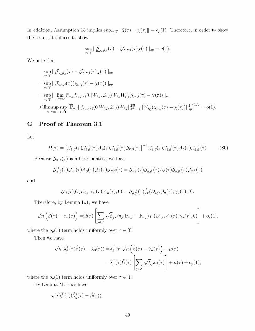
In addition, Assumption 13 implies supτ∈Υ ‖χ(τ)− χ(τ)‖ = op(1). Therefore, in order to show
the result, it suffices to show
supτ∈Υ||J
γ,θ,j(τ)− Jγ,γ,j(τ)χ(τ)||op = o(1).
We note that
supτ∈Υ||J
γ,θ,j(τ)− Jγ,γ,j(τ)χ(τ)||op
= supτ∈Υ||Jγ,γ,j(τ)(χn,j(τ)− χ(τ))||op
= supτ∈Υ|| limn→∞
Pn,jfεi,j(τ)(0|Wi,j, Zi,j)Wi,jW>i,j(χn,j(τ)− χ(τ))||op
≤ lim supn→∞
supτ∈Υ
[Pn,j||fεi,j(τ)(0|Wi,j, Zi,j)Wi,j||22Pn,j||W>
i,j(χn,j(τ)− χ(τ))||2op]1/2
= o(1).
G Proof of Theorem 3.1
Let
Ω(τ) =[J >θ,β(τ)J −1
θ,θ (τ)Aφ(τ)J −1θ,θ (τ)Jθ,β(τ)
]−1 J >θ,β(τ)J −1θ,θ (τ)Aφ(τ)J −1
θ,θ (τ) (80)
Because Jπ,π(τ) is a block matrix, we have
J >π,β(τ)J >θ (τ)Aφ(τ)J θ(τ)Jπ,β(τ) = J >θ,β(τ)J −1θ,θ (τ)Aφ(τ)J −1
θ,θ (τ)Jθ,β(τ)
and
J θ(τ)fτ (Di,j, βn(τ), γn(τ), 0) = J −1θ,θ (τ)fτ (Di,j, βn(τ), γn(τ), 0).
Therefore, by Lemma L.1, we have
√n(β(τ)− βn(τ)
)=Ω(τ)
[∑j∈J
√ξj√nj(Pn,j − Pn,j)fτ (Di,j, βn(τ), γn(τ), 0)
]+ op(1),
where the op(1) term holds uniformly over τ ∈ Υ.
Then we have
√n(λ>β (τ)β(τ)− λ0(τ)) =λ>β (τ)
√n(β(τ)− βn(τ)
)+ µ(τ)
=λ>β (τ)Ω(τ)
[∑j∈J
√ξjZj(τ)
]+ µ(τ) + op(1),
where the op(1) term holds uniformly over τ ∈ Υ.
By Lemma M.1, we have
√nλ>β (τ)(β∗g(τ)− β(τ))
49

=λ>β (τ)Ω(τ)√n
∑j∈J
gjξjnj
∑i∈In,j
fτ (Di,j, βn(τ), γn(τ), 0)
− λ>β (τ)
∑j∈J
Ω(τ)ξjgjJπ,β,j(τ)√n(βr(τ)− βn(τ)) + op(1)
=λ>β (τ)Ω(τ)√n
∑j∈J
gjξjnj
∑i∈In,j
fτ (Di,j, βn(τ), γn(τ), 0)
+ a∗g(τ)µ(τ) + op(1)
where op(1) term holds uniformly over τ ∈ Υ, a∗g(τ) =∑
j∈J ξjgjaj(τ), and the last equality
holds because
λ>β (τ)∑j∈J
Ω(τ)ξjgjJπ,β,j(τ)√n(βr(τ)− βn(τ))
=λ>β (τ)∑j∈J
Ω(τ)ξjgjJθ,β,j(τ)√n(βr(τ)− βn(τ))
=a∗g(τ)√nλ>β (τ)(βr(τ)− βn(τ)) = −a∗g(τ)µ(τ). (81)
Let TQR∞ (g) = supτ∈Υ
[‖λ>β (τ)Ω(τ)
[∑j∈J gj
√ξjZj(τ)
]+∑
j∈J gjξjaj(τ)µ(τ)‖Ar(τ)
]. Then,
we have, uniformly over τ ∈ Υ
TQRn , TQR∗n (g)g∈G (TQR∞ (ιq), TQR∞ (g)g∈G),
where ιq is a q× 1 vector of ones and we use the fact that 1 =∑
j∈J ξjaj(τ). In addition, under
H0, TQR∞ (g)d= TQR∞ (g′). Let k∗ = d|G|(1 − α)e. We order TQR∗n (g)g∈G and TQR∞ (g)g∈G in
ascending order:
(TQR∗n )(1) ≤ · · · ≤ (TQR∗n )(|G|) and (TQR∞ )(1) ≤ · · · ≤ (TQR∞ )|G|.
Then, we have
cQRn (1− α)p−→ (TQR∞ )(k∗)
and
lim supn→∞
P(TQRn > cQRn (1− α)) ≤ lim supn→∞
P(TQRn ≥ cQRn (1− α))
≤P(TQR∞ (ιq) ≥ (TQR∞ )(k∗)
)≤ α +
1
2q−1,
where the second inequality is due to Portmanteau’s theorem (see, e.g., (van der Vaart and
Wellner, 1996), Theorem 1.3.4(iii)), and the third inequality is due to the properties of ran-
domization tests (see, e.g., (Lehmann and Romano, 2006), Theorem 15.2.1) and the facts that
the distribution of TQR∞ (g) is invariant w.r.t. g, TQR∞ (g) = TQR∞ (−g), and TQR∞ (g) 6= TQR∞ (g′) if
50

g /∈ g′,−g′. Similarly, we have
lim infn→∞
P(TQRn > cQRn (1− α)) = lim infn→∞
P(TQRn > (TQR∗n )(k∗)) ≥ P(TQR∞ (ιq) > (TQR∞ )(k∗)
)≥ α− 1
2q−1.
To see the last inequality, we note that TQR∞ (g) = TQR∞ (−g), and TQR∞ (g) 6= TQR∞ (g′) if g /∈g′,−g′. Therefore, ∑
g∈G
1TQR∞ (g) ≤ (TQR∞ )(k∗) ≤ k∗ + 1.
Then, with |G| = 2q, we have
|G|E1TQR∞ (ιq) > (TQR∞ )(k∗) =E∑g∈G
1TQR∞ (g) > (TQR∞ )(k∗)
=|G| − E∑g∈G
1TQR∞ (g) ≤ (TQR∞ )(k∗) ≥ |G| − (k∗ + 1)
≥b|G|αc − 1 ≥ |G|α− 2,
where the first equality holds because TQR∞ (ιq)d= TQR∞ (g) for g ∈ G.
Under H1,n, we still have
lim infn→∞
P(TQRn > cQRn ) ≥ P(TQR∞ (ιq) > (TQR∞ )(k∗)
).
Let Gs = G\Gw, where Gw = g ∈ G : gj = gj′ , ∀j, j′ ∈ Js. We aim to show that, as
infτ∈Υ ||µ(τ)|| → ∞,
P(TQR∞ (ιq) > maxg∈Gs
TQR∞ (g))→ 1. (82)
In addition, we note that |Gs| = |G| − 2q−qs+1 ≥ k∗. This implies as infτ∈Υ ||µ(τ)|| → ∞,
P(TQR∞ (ιq) > (TQR∞ )(k∗)) ≥ P(TQR∞ (ιq) > maxg∈Gs
TQR∞ (g))→ 1.
Therefore, it suffices to establish (82). Note TQR∞ (ιq) ≥ infτ∈Υ ||µ(τ)||Ar(τ) −Op(1) and
maxg∈Gs
TQR∞ (g) ≤ supτ∈Υ,g∈Gs
|∑j∈J
gjξjaj(τ)| supτ∈Υ||µ(τ)||Ar(τ) +Op(1).
Because when g ∈ Gs, the signs of gjj∈Js cannot be the same. In addition, we have∑j∈J ξjaj(τ) =
∑j∈Js ξjaj(τ) = 1, and infτ∈Υ,j∈Js aj(τ) ≥ c > 0. These imply
maxg∈Gs,τ∈Υ
|∑j∈J
gjξjaj(τ)| ≤ 1− 2 minj∈J
ξjc < 1.
Then, as infτ∈Υ ||µ(τ)||2 →∞, we have
infτ∈Υ||µ(τ)||Ar(τ) − (1− 2 min
j∈Jξj) sup
τ∈Υ||µ(τ)||Ar(τ)
51

≥ ( infτ∈Υ
λmin(Ar(τ))− (1− 2 minj∈J
ξjc) infτ∈Υ
λmin(Ar(τ))cµ) infτ∈Υ||µ(τ)||2 →∞
This concludes the proof.
H Proof of Theorem 3.2
We focus on testing the first type of the null hypothesis. Recall Ω(τ) defined in (80),
TQRCR,n = supτ∈Υ||√n(λ>β (τ)β(τ)− λ0(τ))||Ar(τ)
and
TQR∗CR,n(g) = supτ∈Υ||√n(λ>β (τ)(β∗g(τ)− β(τ)))||Ar,CR,g(τ).
Following the proof of Theorem 3.1, we have
√n(λ>β (τ)β(τ)− λ0(τ)) = λ>β (τ)Ω(τ)
[∑j∈J
√ξjZj
]+ µ(τ) + op(1)
and
√n(λ>β (τ)(β∗g (τ)− β(τ)))
=λ>β (τ)Ω(τ)
[∑j∈J
gj√ξjZj(τ)
]− λ>β (τ)
∑j∈J
Ω(τ)ξjgjJπ,β,j(τ)√n(βr(τ)− βn(τ)) + op(1)
=λ>β (τ)Ω(τ)
[∑j∈J
gj√ξjZj(τ)
]+ a∗g(τ)µ(τ) + op(1),
where the op(1) terms in these two displays hold uniformly over τ ∈ Υ.
Next, we derive the limits of A−1r,CR(τ) and (A∗r,CR,g)
−1(τ). Note
A−1r,CR(τ)
=λ>β (τ)Ω(τ)V (τ, τ ′)Ω>(τ)λβ(τ)
=∑j∈J
ξjnjλ>β (τ)Ω(τ)
[Pn,j fτ (Di,j, β(τ), γ(τ), 0)
] [Pn,j fτ ′(Di,j, β(τ ′), γ(τ ′), 0)
]Ω>(τ)λβ(τ).
By Lemma O.1, we have
√njλ
>β (τ)Ω(τ)
[Pn,j fτ (Di,j, β(τ), γ(τ), 0)
]=λ>β (τ)
[Ω(τ)
√njPn,j fτ (Di,j, βn(τ), γn(τ), 0)− aj(τ)Ω(τ)
√njPnfτ (Di,j, βn(τ), γn(τ), 0)
]+ op(1)
=λ>β (τ)Ω(τ)
Zj(τ)− aj(τ)√ξj∑j∈J
ξjZj(τ)
+ op(1),
52

where the op(1) term holds uniformly over τ ∈ Υ. Because q > dr,
infτ∈Υ
λmin
λ>β (τ)Ω(τ)∑
j∈J ξj
[Zj(τ)− aj(τ)
√ξj∑
j∈J√ξ jZj(τ)
]×[Zj(τ)− aj(τ)
√ξj∑
j∈J√ξ jZj(τ)
]>Ω>(τ)λβ(τ)
> 0
with probability one, we have
Ar,CR(τ) =
λ>β (τ)Ω(τ)∑
j∈J ξj
[Zj(τ)− aj(τ)
√ξj∑
j∈J√ξ jZj(τ)
]×[Zj(τ)− aj(τ)
√ξj∑
j∈J√ξ jZj(τ)
]>Ω>(τ)λβ(τ)
−1
+ op(1).
≡Ar,CR(τ) + op(1).
Similarly, we have
(A∗r,CR,g)−1(τ) =λ>β (τ)Ω(τ)V ∗g (τ, τ ′)Ω>(τ)λβ(τ)
=∑j∈J
ξjnjλ>β (τ)Ω(τ)
[Pn,jf
∗τ,g(Di,j)
] [Pn,jf
∗τ,g(Di,j)
]>Ω>(τ)λβ(τ).
Furthermore, Lemma O.1 shows
√njλ
>β (τ)Ω(τ)
[Pn,jf
∗τ,g(Di,j)
]=√njλ
>β (τ)
[gjΩ(τ)Pn,j fτ (Di,j, βn(τ), γn(τ), 0)− gjaj(τ)(βr(τ)− βn(τ))
− Ω(τ)aj(τ)∑j∈J
gjξjPn,j fτ (Di,j, βn(τ), γn(τ), 0) + aj(τ)a∗g(τ)(βr(τ)− βn(τ))
]+ op(1),
=λ>β (τ)Ω(τ)
gjZj(τ)− aj(τ)√ξj∑j∈J
gj
√ξjZj(τ)
+√ξj(gj − a
∗g(τ))aj(τ)µ(τ) + op(1),
where the op(1) term holds uniformly over τ ∈ Υ, a∗g(τ) =∑
j∈J ξjgjaj(τ), and the second
equality holds because
−√njλ>β (τ)(gj − a∗g(τ)
)aj(τ)(βr(τ)− βn(τ)) =
√ξj(gj − a
∗g(τ))aj(τ)µ(τ).
Then, as q > dr,
A∗r,CR,g(τ) = Ar,CR,g(τ) + op(1),
where the op(1) term holds uniformly over τ ∈ Υ and
Ar,CR,g(τ)
=
∑j∈J ξj
λ>β (τ)Ω(τ)
[gjZj(τ)− aj(τ)
√ξj∑
j∈J√ξ jgjZj(τ)
]+√ξj(gj − a∗g(τ))aj(τ)µ(τ)
×λ>β (τ)Ω(τ)
[gjZj(τ)− aj(τ)
√ξj∑
j∈J√ξ jgjZj(τ)
]+√ξj(gj − a∗g(τ))aj(τ)µ(τ)
>−1
.
53

Let
TQRCR,∞(g) = supτ∈Υ
∥∥∥∥∥λ>β (τ)Ω(τ)
[∑j∈J
gj√ξjZj(τ) +
∑j∈J
gjξjaj(τ)µ(τ)
]∥∥∥∥∥Ar,CR,g(τ)
.Because a∗ιq(τ) = 1 and a∗−ιq(τ) = −1, we have,
TQRCR,n, TQR∗CR,n(g)g∈G TQRCR,∞(ιq), TQRCR,∞(g)g∈G.
In addition, because q > dr, under the null, TQRCR,∞(g)d= TQRCR,∞(g′) for any g, g′ ∈ G and
TQRCR,∞(g) = TQRCR,∞(g′) if and only if g ∈ g′,−g′. Then following the exact same argument in
the proof of Theorem 3.1, we have
α− 1
2q−1≤ lim inf
n→∞P(TQRCR,n > cQRCR,n(1− α)) ≤ lim sup
n→∞P(TQRCR,n > cQRCR,n(1− α)) ≤ α +
1
2q−1.
For the power analysis, we still have
lim infn→∞
P(TQRCR,n > cQRn ) ≥ P(TQRCR,∞(ιq) > (TQRCR,∞)(k∗)
).
In addition, we aim to show that, as infτ∈Υ ||µ(τ)|| → ∞, we have
P(TQRCR,∞(ιq) > max
g∈Gs
TQRCR,∞(g)
)→ 1. (83)
Then, given |Gs| = |G|−2q−qs+1 and d|G|(1−α)e ≤ |G|−2q−qs+1, (83) implies, infτ∈Υ ||µ(τ)|| →∞,
P(TQRCR,∞(ιq) > (TQRCR,∞)(k∗)
)> P
(TQRCR,∞(ιq) > max
g∈Gs
TQRCR,∞(g)
)→ 1.
Therefore, it suffices to establish (83). Note that
TQRCR,∞(ιq) = supτ∈Υ
∥∥∥∥∥λ>β (τ)Ω(τ)
[∑j∈J
gj√ξjZj(τ)
]+ µ(τ)
∥∥∥∥∥Ar,CR,ιg (τ)
,where
Ar,CR,ιg(τ) =
∑j∈J ξj
λ>β (τ)Ω(τ)
[gjZj(τ)− aj(τ)
√ξj∑
j∈J√ξ jgjZj(τ)
]×λ>β (τ)Ω(τ)
[gjZj(τ)− aj(τ)
√ξj∑
j∈J√ξ jgjZj(τ)
]>−1
.
We see that Ar,CR,ιg(τ) is independent of µ. In addition, with probability one, we have
infτ∈Υ
λmin(Ω>(τ)λ>β (τ)Ar,CR,ιg(τ)λβ(τ)Ω(τ)) > 0.
Therefore, for any e > 0, we can find a constant c > 0 such that with probability greater than
54

1− e,
TQRCR,∞(ιq) ≥ c infτ∈Υ||µ(τ)||2 −Op(1). (84)
On the other hand, for g ∈ Gs, we can write TQRCR,∞(g) as
TQRCR,∞(g) = supτ∈Υ
(N0,g(τ) + c0,g(τ)µ(τ))>
[∑j∈J
ξj(Nj,g(τ) + cj,g(τ)µ(τ))(Nj,g(τ) + cj,g(τ)µ(τ))>
]−1
× (N0,g(τ) + c0,g(τ)µ(τ))
,
where
N0,g(τ) = λ>β (τ)Ω(τ)
[∑j∈J
gj√ξjZj(τ)
],
Nj,g(τ) = λ>β (τ)Ω(τ)
gjZj(τ)− aj(τ)√ξj∑j∈J
√ξ jgjZj(τ)
, j ∈ J,
c0,g(τ) = a∗g(τ),
cj,g(τ) =√ξj(gj − a
∗g(τ))aj(τ), j ∈ J.
We claim that for g ∈ Gs, cj,g(τ) 6= 0 for some j ∈ Js. To see this claim, suppose it does not
hold. Then, it implies gj = a∗g(τ) for all j ∈ Js, i.e., for all j ∈ Js, gj shares the same sign. This
contradicts with the definition of Gs. This claim and the fact that infτ∈Υ,j∈Js |aj(τ)| ≥ c0 > 0
further imply that
infτ∈Υ,g∈Gs
∑j∈J
ξjc2j,g(τ)
≥ (c20 minj∈J
ξ2j ) max((1− a∗g(τ))2, (1 + a∗g(τ))2)
≥c2
0 minj∈J ξ2j
2
[(1− a∗g(τ))2 + (1 + a∗g(τ))2
]≥ c2
0 minj∈J
ξ2j > 0.
In addition, we have∑j∈J
ξj(Nj,g(τ) + cj,g(τ)µ(τ))(Nj,g(τ) + cj,g(τ)µ(τ))>
=∑j∈J
ξjNj,g(τ)N>j,g(τ) +∑j∈J
ξjcj,g(τ)Nj,g(τ)µ(τ)>
+∑j∈J
ξjcj,g(τ)µ(τ)Nj,g(τ)> + (∑j∈J
ξjc2j,g(τ))µ(τ)µ(τ)>
≡M1 +M2µ(τ)> + µ(τ)M>2 + c2µ(τ)µ(τ)>,
55

where we denote
M1 =∑j∈J
ξjNj,g(τ)N>j,g(τ), M2 =∑j∈J
ξjcj,g(τ)Nj,g(τ), and c2 =∑j∈J
ξjc2j,g(τ).
For notation ease, we suppress the dependence of (M1,M2, c) on (g, τ). Then, we have
M1 +M2µ(τ)> + µ(τ)M>2 + c2µ(τ)µ(τ)> = M1 −
M2M>2
c2 +
(M2
c+ cµ(τ)
)(M2
c+ cµ(τ)
)>.
Note for any dr × 1 vector u, by the Cauchy-Schwarz inequality,
u>(M1 −
M2M>2
c2
)u =
∑j∈J
ξj(u>Nj,g(τ))2 −
(∑j∈J ξju
>Nj,g(τ)cj,g(τ))2∑
j∈J ξjc2j,g(τ)
≥ 0,
where the equal sign holds if and only if there exist (u, τ, g) ∈ <dr ×Υ× (Gs)) such that
u>N1,g(τ)
c1,g(τ)= · · · = u>Nq,g(τ)
cq,g(τ),
which has probability zero if q > dr. Therefore, the matrix M ≡M1 − M2M>2c2
is invertible with
probability one. Specifically, denote M as Mg(τ) to highlight its dependence on (g, τ). We have
sup(g,τ)∈Gs×Υ(λmin(M(g, τ)))−1 = Op(1). In addition, denote M2
c+ cµ(τ) as V, which is a dr × 1
vector. Then, we have[∑j∈J
ξj(Nj,g(τ) + cj,g(τ)µ(τ))(Nj,g(τ) + cj,g(τ)µ(τ))>
]−1
= [M + VV>]−1
= M−1 −M−1V(1 + V>M−1V)−1V>M−1,
where the second equality is due to the Sherman-Morrison-Woodbury formula.
Next, we note that
N0,g(τ) + c0,g(τ)µ(τ) = N0,g(τ) + c0,g(τ)
(Vc− M2
c2
)≡M0 +
c0,g(τ)
cV,
where
M0 = N0,g(τ)− c0,g(τ)M2
c2 = N0,g(τ)−c0,g(τ)(
∑j∈J ξjcj,q(τ)Nj,g(τ))∑j∈J ξjc
2j,g(τ)
.
With these notations, we have
(N0,g(τ) + c0,g(τ)µ(τ))>
[∑j∈J
ξj(Nj,g(τ) + cj,g(τ)µ(τ))(Nj,g(τ) + cj,g(τ)µ(τ))>
]−1
56

× (N0,g(τ) + c0,g(τ)µ(τ))
=
(M0 +
c0,g(τ)
cV)>
(M−1 −M−1V(1 + V>M−1V)−1V>M−1)
(M0 +
c0,g(τ)
cV)
≤ 2M>0 (M−1 −M−1V(1 + V>M−1V)−1V>M−1)M0
+2c2
0,g(τ)
c2 V>(M−1 −M−1V(1 + V>M−1V)−1V>M−1)V
≤ 2M>0 M−1M0 +2c2
0,g(τ)
c2
V>M−1V1 + V>M−1V
≤ 2M>0 M−1M0 +2c2
0,g(τ)
c2
≤ 2(λmin(M(g, τ)))−1
∥∥∥∥∥N0,g(τ)−c0,g(τ)(
∑j∈J ξjcj,q(τ)Nj,g(τ))∑j∈J ξjc
2j,g(τ)
∥∥∥∥∥2
+2c2
0,g(τ)∑j∈J ξjc
2j,g(τ)
≡ C(g, τ),
where the first inequality is due to the fact that (u + v)>A(u + v) ≤ 2(u>Au + v>Av) for
some dr × dr positive semidefinite matrix A and u, v ∈ <dr , the second inequality holds due to
the fact that M−1V(1 + V>M−1V)−1V>M−1 is positive semidefinite, the third inequality holds
because V>M−1V is a nonnegative scalar, and the last inequality holds by substituting in the
expressions for M0 and c and denoting M as M(g, τ). By taking the supremum over τ ∈ Υ first
followed by g ∈ Gs, we have
maxg∈Gs
TQRCR,∞(g) ≤ sup(g,τ)∈Gs×Υ
C(g, τ) = Op(1). (85)
Combining (84) and (85), we have, as infτ∈Υ ||µ(τ)|| → ∞,
P(TQRCR,∞(ιq) > max
g∈Gs
TQRCR,∞(g)
)≥ P
(c infτ∈Υ||µ(τ)||2 −Op(1) > sup
(g,τ)∈Gs×Υ
C(g, τ)
)− e→ 1− e.
As e is arbitrary, we have established (83). This concludes the proof.
I Proof of Theorem 3.3
We focus on the case when Assumption 12(ii) holds. The proof for the case with Assumption
12(i) is similar but simpler, and thus, is omitted for brevity. We divide the proof into three
steps. In the first step, we derive the limit distribution of ARQRCR,n. In the second step, we derive
the limit distribution of ARQR∗CR,n(g). In the third step, we prove the desired result. Throughout
the proof, we impose the null that βn(τ) = β0(τ) for τ ∈ Υ.
57

Step 1. By Lemma K.1 with bn(τ) = βn(τ) = β0(τ), we have
√nθ(β0(τ), τ) =ω [Γ1(β0(τ), τ)]−1√n [In(τ) + IIn(bn(τ), τ) + op(1)− Γ2(β0(τ), τ)(β0(τ)− βn(τ))]
=ω [Jπ,π(τ)]−1√nIn(τ) + op(1), (86)
where the op(1) terms hold uniformly over τ ∈ Υ and
In(τ) = (Pn − Pn)fτ (D, βn(τ), γn(τ), 0).
In addition, note
A−1CR(τ) =
∑j∈J
ξjnjωJ −1π,π(τ)
[Pn,j fτ (Di,j, β0(τ), γ(β0(τ), τ))
]×[Pn,j fτ (Di,j, β0(τ), γ(β0(τ), τ))
]>J −1π,π(τ)ω>
Furthermore, we have
Pn,j fτ (Di,j, β0(τ), γ(β0(τ), τ), 0)
=(Pn,j − Pn,j)fτ (Di,j, β0(τ), γ(β0(τ), τ), 0) + Pn,j fτ (Di,j, β0(τ), γ(β0(τ), τ), 0)
=(Pn,j − Pn,j)fτ (Di,j, β0(τ), γ(β0(τ), τ), 0) + Pn,j fτ (Di,j, β0(τ), γ(β0(τ), τ), 0) + op(n−1/2)
=Pn,jfτ (Di,j, βn(τ), γn(τ), 0)− Jπ,π,j(τ)
(γ(βn(τ), τ)− γn(τ)
0
)+ op(n
−1/2)
=Op(n−1/2),
where both the Op(n−1/2) and op(n
−1/2) terms hold uniformly over τ ∈ Υ, the second equality
is due to Assumption 6(ii), the third equality is due to Assumption 6(iii) and the fact that
supτ∈Υ||γ(β0(τ), τ)− γn(τ)||2 = Op(n
−1/2)
as shown in Lemma L.2, and the last equality is due to Lemma L.2.
Recall ω = (0dφ×dw , Idφ×dφ). Then, by Lemma K.1, we have
ωJ −1π,π(τ)
[Pn,j fτ (Di,j, β0(τ), γ(β0(τ), τ))
]=ωJ −1
π,π(τ)
[Pn,jfτ (Di,j, β0(τ), γn(τ), 0)− Jπ,π,j(τ)
(γ(β0(τ), τ)− γn(τ)
0
)]+ op(n
−1/2)
=J −1θ,θ (τ)
[Pn,j fτ (Di,j, β0(τ), γn(τ), 0)
]+ op(n
−1/2),
where the op(n−1/2) terms hold uniformly over τ ∈ Υ and the second inequality holds because
under Assumption 7(i),
ωJ −1π,π(τ)Jπ,π,j(τ)
(γ(βn(τ), τ)− γn(τ)
0
)= 0.
58

Then we have
√nθ(β0(τ), τ) = J −1
θ,θ (τ)∑j∈J
√ξjZj(τ) + op(1), (87)
√njωJ −1
π,π(τ)[Pn,j fτ (Di,j, βn(τ), γ(βn(τ), τ))
]= J −1
θ,θ (τ)Zj(τ) + op(1),
and
A−1CR(τ) =
∑j∈J
ξjJ −1θ,θ (τ)Zj(τ)Z>j (τ)J −1
θ,θ (τ) + op(1),
where the op(1) term hold uniformly over τ ∈ Υ. When q > dφ,∑
j∈J ξjJ−1θ,θ (τ)Zj(τ)Z>j (τ)J −1
θ,θ (τ)
is invertible with probability one, we have
ACR(τ) =
[∑j∈J
ξjJ −1θ,θ (τ)Zj(τ)Z>j (τ)J −1
θ,θ (τ)
]−1
+ op(1), (88)
where the op(1) term hold uniformly over τ ∈ Υ. Then, combining (86), (87), and (88), we
have
n(ARQRCR,n)2
= supτ∈Υ
[∑j∈J
√ξjZ
>j (τ)
]J −1θ,θ (τ)
[∑j∈J
ξjJ −1θ,θ (τ)Zj(τ)Z>j (τ)J −1
θ,θ (τ)
]−1
J −1θ,θ (τ)
[∑j∈J
√ξjZj(τ)
]+ op(1).
Step 2. Next, we consider the limit distribution of the bootstrap test statistic. By the
sub-gradient condition of (31), we have
op(1/√n) =Pnfτ (Di,j, β0(τ), γ∗g(τ), θ∗g(τ)) +
1
n
∑j∈J
gj∑i∈In,j
fτ (Di,j, β0(τ), γ(β0(τ), τ), 0), (89)
where the op(1/√n) term on the LHS of the above display holds uniformly over τ ∈ Υ. In
addition,
Pnfτ (Di,j, β0(τ), γ∗g(τ), θ∗g(τ))
=In(τ) + IIn,g(β0(τ), τ)− Γ1,g(β0(τ), τ)
(γ∗g(τ)− γn(τ)
θ∗g(τ)
), (90)
where
In(τ) = (Pn − Pn)fτ (Di,j, β0(τ), γn(τ), 0),
IIn,g(β0(τ), τ) =∑j∈J
ξj(Pn,j − Pn,j)(fτ (Di,j, β0(τ), γ∗g(τ), θ∗g(τ))− fτ (Di,j, β0(τ), γn(τ), 0)
)
59

Γ1,g(β0(τ), τ) =∑j∈J
ξjnj
∑i∈In,j
Efεi,j(τ)(δi,j,g(τ)|Wi,j, Zi,j)Ψi,j(τ)Ψ>i,j(τ),
and
δi,j,g(τ) ∈ (0,W>i,j(γ
∗g(τ)− γn(τ)) + Φ>i,j(τ)θ∗g(τ)).
Following the same argument in Step 1 of the proof of Lemma M.1, we have
supτ∈Υ
(||γ∗g(τ)− γn(τ)||2 + ||θ∗g(τ)||2
)= op(1),
supτ∈Υ
√n||IIn,g(βn(τ), τ)||2 = op(1),
and
supτ∈Υ,j∈J
∥∥∥∥∥∥ 1
nj
∑i∈In,j
Efεi,j(τ)(δi,j,g(τ)|Wi,j, Zi,j)Ψi,j(τ)Ψ>i,j(τ)− Jπ,π(τ)
∥∥∥∥∥∥op
= op(1).
Note here, to derive the above three displays, we do not need to impose Assumption 8(i)–8(iii)
as did in Lemma M.1 because β0(τ) = βn(τ) under the null. In addition, we have
1
n
∑j∈J
gj∑i∈In,j
fτ (Di,j, β0(τ), γ(β0(τ), τ), 0)
=1
n
∑j∈J
gj∑i∈In,j
(fτ (Di,j, β0(τ), γ(β0(τ), τ), 0)− fτ (Di,j, β0(τ), γn(τ), 0)
)+
1
n
∑j∈J
gj∑i∈In,j
fτ (Di,j, β0(τ), γn(τ), 0)
=1
n
∑j∈J
gj
∑i∈In,j
fτ (Di,j, β0(τ), γn(τ), 0)− Jπ,π,j(τ)
(γ(β0(τ), τ)− γn(τ)
0
)+ op(n−1/2).
where the op(n−1/2) term holds uniformly over τ ∈ Υ. Therefore, we have(
γ∗g(τ)− γn(τ)
θ∗g(τ)
)
=J −1π,π(τ)
In(τ) +1
n
∑j∈J
gj
∑i∈In,j
fτ (Di,j, βn(τ), γn(τ), 0)− Jπ,π,j(τ)
(γ(β0(τ), τ)− γn(τ)
0
)+ op(n
−1/2)
and
√nθ∗g(τ) = ωJ −1
π,π(τ)
1√n
∑j∈J
(1 + gj)∑i∈In,j
fτ (Di,j, βn(τ), γn(τ), 0)
+ op(1),
60

where the op(1) term holds uniformly over τ ∈ Υ and the second display holds because under
Assumption 7(i), we have
ωJ −1π,π(τ)Jπ,π,j(τ)
(γ(β0(τ), τ)− γn(τ)
0
)= 0.
Therefore, we have
√n(θ∗g(τ)− θ(β0(τ), τ)) =ωJ −1
π,π(τ)
1√n
∑j∈J
gj∑i∈In,j
fτ (Di,j, βn(τ), γn(τ), 0)
+ op(1)
=J −1θ,θ (τ)
1√n
∑j∈J
gj∑i∈In,j
fτ (Di,j, βn(τ), γn(τ), 0)
+ op(1),
where the op(1) term holds uniformly over τ ∈ Υ. We further define
ARQRCR,∞(g)
= supτ∈Υ
∑j∈J
√ξjgjZj(τ)J −1
θ,θ (τ)
[∑j∈J
ξjJ −1θ,θ (τ)gjZj(τ)gjZ>j (τ)J −1
θ,θ (τ)
]−1
J −1θ,θ (τ)
[∑j∈J
√ξjgjZj(τ)
]1/2
.
Then, we have, under the null,
(√nARQR
CR,n, √nARQR∗
CR,n(g)g∈G) (ARQRW,∞(ιq), ARQR
CR,∞(g)g∈G).
The distribution of ARQRCR,∞(g) is invariant in g, and ARQR
CR,∞(g) = ARQRCR,∞(g′) if and only if
g ∈ g′,−g′. Then, by the same argument in the proofs of Theorem 3.1, we have
α− 1
2q−1≤ lim inf
n→∞P(ARQR
CR,n > cQRAR,CR,n(1− α)) ≤ lim supn→∞
P(ARQRCR,n > cQRAR,CR,n(1− α)) ≤ α +
1
2q−1.
J Proof of Proposition A.2
We have
sup∥∥∥Pn,jfεi,j(τ)(δi,j(v, τ)|Wi,j, Zi,j)V
2i,j(τ)Wi,jΦ
>i,j(τ)
∥∥∥op
≤ sup∥∥∥Pn,jfεi,j(τ)(δi,j(v, τ)|Wi,j, Zi,j)V
2i,j(τ)Wi,jΦ
>i,j(τ)− J
γ,θ,j(τ)∥∥∥op
+ sup∥∥[Pn,jfεi,j(τ)(δi,j(v, τ)|Wi,j, Zi,j)V
2i,j(τ)Wi,jW
>i,j(τ)− Jγ,γ,j(τ)
]χj(τ)
∥∥op
+ supτ∈Υ||Jγ,γ,j(τ)χj(τ)− J
γ,θ,j(τ)||op + sup
τ∈Υ||J
γ,θ,j(τ)− J
γ,θ,j(τ)||op
+ supτ∈Υ
∥∥∥[Jγ,γ,j(τ)− Jγ,γ,j(τ)]χj(τ)
∥∥∥op
61

where the suprema in the first three lines are taken over j ∈ J, ||v||2 ≤ δ, τ ∈ Υ for v =
(v>b , v>r , v
>t )>. We note that, by Assumption 14, by letting n→∞ followed by δ → 0,
sup∥∥∥Pn,jfεi,j(τ)(δi,j(v, τ)|Wi,j, Zi,j)V
2i,j(τ)Wi,jψ
>i,j
(τ)− Jγ,θ,j
(τ)∥∥∥op
p−→ 0 and
sup∥∥[Pn,jfεi,j(τ)(δi,j(v, τ)|Wi,j, Zi,j)V
2i,j(τ)Wi,jW
>i,j(τ)− Jγ,γ,j(τ)
]χj(τ)
∥∥op
p−→ 0.
Assumption 14 also implies
supτ∈Υ||J
γ,θ,j(τ)− J
γ,θ,j(τ)||op + sup
τ∈Υ
∥∥∥Jγ,γ,j(τ)− Jγ,γ,j(τ)∥∥∥op
= op(1).
Therefore, in order to show the result, it suffices to show
supτ∈Υ||χj(τ)||op = Op(1) (91)
and
Jγ,γ,j(τ)χj(τ)− Jγ,θ,j
(τ) = 0. (92)
To see (91), we note that Assumption 14(ii) implies the generalized inverse is continuous at
Jγ,γ,j(τ) uniformly over τ ∈ Υ. Therefore, by the continuous mapping theorem, we have
||J −γ,γ,j(τ)− J −γ,γ,j(τ)||op = op(1),
and thus
supτ∈Υ||χj(τ)||op ≤ sup
τ∈Υ||χj(τ)− Jγ,γ,j(τ)J −γ,γ,j(τ)J −γ,γ,j(τ)J
γ,θ,j(τ)||op
+ supτ∈Υ||Jγ,γ,j(τ)J −γ,γ,j(τ)J −γ,γ,j(τ)J
γ,θ,j(τ)||op = Op(1).
To show (92), we define Wj = (W1,jK1/2(εi,jh
)h−1/2, · · · ,Wnj ,jK
1/2(εnj,j
h
)h−1/2)> and
Ij = (Φ1,j(τ)K1/2(εi,jh
)h−1/2, · · · , Φnj ,j(τ)K1/2
(εnj,j
h
)h−1/2)>. Then, we have
Jγ,γ,j(τ) =1
njX>j Xj and Jγ,θ,j(τ) =
1
njX>j Ij.
Define the singular value decomposition of Xj as Xj = U>j ΣjVj, where Uj and Vj are nj × njand dw×dw orthonormal matrices and Σj is a nj×dw matrix with the first R diagonal elements
being positive and all the rest entries in the matrix being zero. Then, we have
Jγ,γ,j(τ)χj(τ) =1
njX Tj XjX T
j Xj(X Tj Xj
)− (X Tj Xj
)−X>j Ij=
1
njV >j (Σ>j Σj)(Σ
>j Σj)(Σ
>j Σj)
−(Σ>j Σj)−Σ>j UjIj
=1
njV >j
(IR 0R×(dw−R)
0(dw−R)×R 0(dw−R)×(dw−R)
)Σ>j UjIj
62

=1
njV >j Σ>j UjIj
=Jγ,θ,j(τ),
where we use the fact that (IR 0R×(dw−R)
0(dw−R)×R 0(dw−R)×(dw−R)
)Σ>j = Σ>j .
This concludes the proof.
K Linear Expansion of γ(bn(τ), τ)
Lemma K.1. Let B(δ) = b(·) ∈ ι∞q (Υ) : supτ∈Υ ||b(τ)− βn(τ)||2 ≤ δ. Suppose Assumptions
5 and 6 hold. and bn(τ) as a generic point in B(δ). Then, for any ε > 0, there exists δ and
constants c′, c > 0 that are independent of (n, δ, ε, δ) such that for δ ≤ δ, with probability greater
than 1− cε,(√n (γ(bn(τ), τ)− γn(τ))√nθ(bn(τ), τ)
)= [Γ1(bn(τ), τ)]−1√n
[In(τ) + IIn(bn(τ), τ) + op(1/
√n)− Γ2(bn(τ), τ)(bn(τ)− βn(τ))
](93)
where the op(1/√n) term on the RHS of the above display holds uniformly over τ ∈ Υ, bn(·) ∈
B(δ),
In(τ) = (Pn − Pn)fτ (D, βn(τ), γn(τ), 0), supτ∈Υ||√nIn(τ)||2 = Op(1),
IIn(bn(τ), τ) = (Pn − Pn)(fτ (D, bn(τ), γ(bn(τ), τ), θn(bn(τ), τ))− fτ (D, βn(τ), γn(τ), 0)
),
supbn(·)∈B(δ),τ∈Υ
||√nIIn(bn(τ), τ)||2 ≤ c′ε,
Γ1(bn(τ), τ) = Pnfεi,j(τ)(δi,j(τ)|Wi,j, Zi,j)Ψi,j(τ)Ψ>i,j(τ), supbn(·)∈B(δ),τ∈Υ
||Γ1(bn(τ), τ)− Jπ,β(τ)||op ≤ ε,
Γ2(bn(τ), τ) = Pnfεi,j(τ)(δi,j(τ)|Wi,j, Zi,j)Ψi,j(τ)X>i,j, supbn(·)∈B(δ),τ∈Υ
||Γ2(bn(τ), τ)− Jπ,β(τ)||op ≤ ε,
and δi,j(τ) ∈ (0, X>i,j(bn(τ)−βn(τ))+W>i,j(γ(bn(τ), τ)−γn(τ))+Φ>i,j(τ)θ(bn(τ), τ)), where || · ||op
denotes the matrix operator norm.
Proof. The subgradient condition for (γ(bn(τ), τ), θ(bn(τ), τ)) implies
op(1/√n) =Pnfτ (Di,j, bn(τ), γ(bn(τ), τ), θ(bn(τ), τ))
63

=(Pn − Pn)fτ (Di,j, bn(τ), γ(bn(τ), τ), θ(bn(τ), τ)) + Pnfτ (Di,j, bn(τ), γ(bn(τ), τ), θ(bn(τ), τ))
=(Pn − Pn)fτ (Di,j, βn(τ), γn(τ), 0)
+ (Pn − Pn)(fτ (Di,j, bn(τ), γ(bn(τ), τ), θ(bn(τ), τ))− fτ (Di,j, βn(τ), γn(τ), 0)
)+ Pnfτ (Di,j, bn(τ), γ(bn(τ), τ), θ(bn(τ), τ))
=In(τ) + IIn(bn(τ), τ) + IIIn(bn(τ), τ), (94)
where the op(1/√n) term on the LHS of the above display holds uniformly over τ ∈ Υ, bn(·) ∈
B(δ). For the first term, we note that Pnfτ (Di,j, βn(τ), γn(τ), 0) = 0. Then, by Assumption
6(vi), we have,
supτ∈Υ||√nIn(τ)||2 = Op(1).
For the second term, note
supτ∈Υ||γ(bn(τ), τ)− γn(τ)||2
≤ supτ∈Υ,b∈B
||γ(b, τ)− γn(b, τ)||2 + supτ∈Υ,b,b′∈B,||b−b′||2≤δ
||γn(b, τ)− γn(b′, τ)||2
≤ supτ∈Υ,b∈B
||γ(b, τ)− γn(b, τ)||2 + supτ∈Υ,b,b′∈B,||b−b′||2≤δ
||γ∞(b, τ)− γ∞(b′, τ)||2
+ 2 supτ∈Υ,b∈B
||γ∞(b, τ)− γn(b, τ)||2,
where the RHS of the above display vanishes as n → ∞ followed by δ ↓ 0. Therefore, for any
δ′ > 0 and ε > 0, there exist n and δ such that for n ≥ n and δ ≤ δ, with probability greater
than 1− ε,
supτ∈Υ||γ(bn(τ), τ)− γn(τ)||2 ≤ δ′.
Similarly, we have
supτ∈Υ||θ(bn(τ), τ)− 0||2 ≤ δ′.
Then, for any ε > 0, there exist n and δ such that for n ≥ n and δ′, δ ≤ δ, with probability
greater than 1− ε, we have,
supbn(·)∈B(δ),τ∈Υ
||√nIIn(bn(τ), τ)||2
≤ sup||v||2≤2δ′+δ
∥∥∥∥√n(Pn − Pn)
(fτ (Di,j, βn(τ) + vb, γn(τ) + vr, vt)− fτ (Di,j, βn(τ), γn(τ), 0)
)∥∥∥∥2
.
Then, by Assumption 6(ii), for any ε > 0, there exist n and δ such that for n ≥ n and δ, δ′ ≤ δ,
64

we have, with probability greater than 1− cε,
supbn(·)∈B(δ),τ∈Υ
||√nIIn(bn(τ), τ)||2 ≤ c′ε,
for some constants (c, c′) that are independent of (n, δ, δ′, ε).
For the third term in (94), we have
Pnfτ (Di,j, bn(τ), γ(bn(τ), τ), θ(bn(τ), τ))
=∑j∈J
ξjPn,j(τ − 1yi,j −X>i,jbn(τ)−W>i,j γ(bn(τ), τ)− Φ>i,j(τ)θ(bn(τ), τ) ≤ 0)Ψi,j(τ)
=− Pn,jfεi,j(τ)(δi,j(τ)|Wi,j, Zi,j)Ψi,j(τ)X>i,j(bn(τ)− βn(τ))
− Pn,jfεi,j(τ)(δi,j(τ)|Wi,j, Zi,j)Ψi,j(τ)Ψ>i,j(τ)
(γ(bn(τ), τ)− γn(τ)
θ(bn(τ), τ)
), (95)
where δi,j(τ) ∈ (0, X>i,j(bn(τ)− βn(τ)) +W>i,j(γ(bn(τ), τ)− γn(τ)) + Φ>i,j(τ)θ(bn(τ), τ)). For any
ε > 0, there exist n and δ such that for n ≥ n and δ, δ′ ≤ δ, we have, with probability greater
than 1− cε,
supτ∈Υ
(||bn(τ)− βn(τ)||2 + ||γ(bn(τ), τ)− γn(τ)||2 + ||θ(bn(τ), τ)||2
)≤ δ + 2δ′.
This implies, with probability greater than 1− cε,
supbn(·)∈B(δ),τ∈Υ,j∈J
||Γ2(bn(τ), τ)− Jπ,β(τ)||op
≤(
maxj∈J
ξj
)sup
bn(·)∈B(δ),τ∈Υ,j∈J
∥∥∥Pn,jfεi,j(τ)(δi,j(τ)|Wi,j, Zi,j)Ψi,j(τ)X>i,j − Jπ,β(τ)∥∥∥op
≤(
maxj∈J
ξj
)sup
∥∥∥Pn,jfεi,j(τ)(δi,j(v, τ)|Wi,j, Zi,j)Ψi,j(τ)X>i,j − Jπ,β,j(τ)∥∥∥op,
where the second supremum in the second inequality is taken over (j, v, τ) : j ∈ J, ||v||2 ≤δ + 2δ′, τ ∈ Υ. Then, Assumption 6(iii) implies, with probability greater than 1− cε,
supbn(·)∈B(δ),τ∈Υ
||Γ2(bn(τ), τ)− Jπ,β(τ)||op ≤ ε.
Similarly, we have, with probability greater than 1− cε,
supbn(·)∈B(δ),τ∈Υ
||Γ1(bn(τ), τ)− Jπ,π(τ)||op ≤ ε.
Then, by Assumption 6 and the fact that ε can be made arbitrarily small, we have, with
probability greater than 1− cε, Γ1(bn(τ), τ) is invertible. Therefore, (94) implies, with proba-
bility greater than 1− cε,(√n (γ(bn(τ), τ)− γn(τ))√nθ(bn(τ), τ)
)
65

= [Γ1(bn(τ), τ)]−1√n[In(τ) + IIn(bn(τ), τ) + op(1/
√n)− Γ2(bn(τ), τ)(bn(τ)− βn(τ))
]where the op(1/
√n) term on the RHS of the above display holds uniformly over τ ∈ Υ, bn(·) ∈
B(δ).
L Technical Results for the IVQR Estimator
Lemma L.1. Suppose Assumptions 5, 6, and 8(i)–8(iii) hold. Then,√n(β(τ)− βn(τ)
)√n (γ(τ)− γn(τ))√nθ(τ)
=
[J >π,β(τ)J >θ (τ)Aφ(τ)J θ(τ)Jπ,β(τ)
]−1
J >π,β(τ)J >θ (τ)Aφ(τ)J θ(τ)
J π,π(τ)
[Idw+dφ − Jπ,β(τ)
[J >π,β(τ)J >θ (τ)Aφ(τ)J θ(τ)Jπ,β(τ)
]−1
J >π,β(τ)J >θ (τ)Aφ(τ)J θ(τ)
]
×√nPnfτ (Di,j, βn(τ), γn(τ), 0) + op(1),
where op(1) term holds uniformly over τ ∈ Υ.
Proof. We divide the proof into three steps. In the first step, we show (β(τ), γ(τ), θ(τ)) are
consistent. In the second step, we derive convergence rates of (β(τ), γ(τ), θ(τ)). In the third
step, we derive linear expansions for (β(τ), γ(τ), θ(τ)).
Step 1. We first show the consistency of (β(τ), γ(τ), θ(τ)). Note by construction, we have
γ(βn(τ), τ) = γn(τ), θn(βn(τ), τ) = 0, γ(τ) = γ(β(τ), τ), and θ(τ) = θ(β(τ), τ). By Kato (2009,
Theorem 1) and the fact that both Qn(b, r, t, τ) and Qn(b, r, t, τ) are convex, we have
sup(b,τ)∈B×Υ
(||γ(b, τ)− γn(b, τ)||2 + ||θ(b, τ)− θn(b, τ)||2
)= op(1).
Similarly, we have
sup(b,τ)∈B×Υ
(||γ∞(b, τ)− γn(b, τ)||2 + ||θ∞(b, τ)− θn(b, τ)||2) = o(1).
This implies
sup(b,τ)∈B×Υ
∣∣∣||θ(b, τ)||Aφ(τ) − ||θ∞(b, τ)||Aφ(τ)
∣∣∣ = op(1)
and 0 = limn→∞ θn(βn(τ), τ) = θ∞(β0(τ), τ), which implies ||θ∞(b, τ)||Aφ(τ) is uniquely mini-
mized at b = β0(τ). Then, Chernozhukov and Hansen (2006, Lemma B.1) implies
supτ∈Υ||β(τ)− β0(τ)||2 = op(1),
66

and thus,
supτ∈Υ||β(τ)− βn(τ)||2 = op(1).
Then, we have
supτ∈Υ||γ(β(τ), τ)− γn(τ)||2 ≤ sup
τ∈Υ,b∈B||γ(b, τ)− γ∞(b, τ)||2 + sup
τ∈Υ||γ∞(β(τ), τ)− γ∞(βn(τ), τ)||2 = op(1),
and similarly,
supτ∈Υ||θ(β(τ), τ)− 0||2 = op(1).
Step 2. We derive the convergence rates of β(τ), γ(τ), and θ(τ). Let B(δ) = b(·) ∈ι∞q (Υ) : supτ∈Υ ||b(τ)− βn(τ)||2 ≤ δ. For any δ > 0, we have β(·) ∈ B(δ) w.p.a.1. Let bn(τ) be
a generic point in B(δ). Recall ω = (0dw×dφ , Idφ). Then, Lemma K.1 implies, with probability
greater than 1− cε,
||√nθ(bn(τ), τ)||2
Aφ(τ)
=n [In(τ) + IIn(bn(τ), τ) +Op(1/n)− Γ2(bn(τ), τ)(bn(τ)− βn(τ))]>
× [Γ1(bn(τ), τ)]−1 ω>Aφ(τ)ω [Γ1(bn(τ), τ)]−1
× [In(τ) + IIn(bn(τ), τ) +Op(1/n)− Γ2(bn(τ), τ)(bn(τ)− βn(τ))]>
≥n(bn(τ)− βn(τ))>
Γ>2 (bn(τ), τ) [Γ1(bn(τ), τ)]−1 ω>Aφ(τ)ω [Γ1(bn(τ), τ)]−1 Γ2(bn(τ), τ)
(bn(τ)− βn(τ))
−Op(1),
where the Op(1) term on the RHS of the above display holds uniformly over τ ∈ Υ, bn(·) ∈ B(δ).
In addition, Lemma K.1 implies that there exists a constant C > 0 such that for any ε > 0,
with probability greater than 1− cε
supbn(·)∈B(δ),τ∈Υ
∥∥∥∥Γ>2 (bn(τ), τ) [Γ1(bn(τ), τ)]−1 ω>Aφ(τ)ω [Γ1(bn(τ), τ)]−1 Γ2(bn(τ), τ)
− J >π,β(τ)J −1θ,θ (τ)TAφ(τ)J −1
θ,θ (τ)Jπ,β(τ)
∥∥∥∥op
≤ Cε.
Therefore, by Assumption 6, there exists a constant c independent of τ and βn(·) such that
n(bn(τ)− βn(τ))>
Γ>2 (bn(τ), τ) [Γ1(bn(τ), τ)]−1 ω>Aφ(τ)ω [Γ1(bn(τ), τ)]−1 Γ2(bn(τ), τ)
(bn(τ)− βn(τ))
−Op(1)
≥c||√n(bn(τ)− βn(τ))||22 −Op(1),
where the Op(1) term on the RHS of the above display holds uniformly over τ ∈ Υ, bn(·) ∈ B(δ).
67

On the other hand, we have β(τ) ∈ B(δ) w.p.a.1 for any δ > 0 and
||√nθ(β(τ), τ)||Aφ(τ) ≤ ||
√nθ(βn(τ), τ)||Aφ(τ) = Op(1),
where the Op(1) term on the RHS of the above display holds uniformly over τ ∈ Υ, b(·) ∈ B(δ).
This implies, for any ε > 0, there exist n and δ such that for n ≥ n and δ, δ′ ≤ δ, we have, with
probability greater than 1− cε,
c||√n(β(τ)− βn(τ))||22 −Op(1) ≤ ||
√nθ(β(τ), τ)||Aφ(τ) ≤ Op(1),
where the Op(1) term on the RHS of the above display holds uniformly over τ ∈ Υ. This further
implies
supτ∈Υ||√n(β(τ)− βn(τ))||2 = Op(1). (96)
Plugging (96) into (93), we obtain that
supτ∈Υ||√n(γ(τ)− γn(τ))||2 = Op(1) and sup
τ∈Υ||√n(θ(τ)− 0)||2 = Op(1).
Step 3. Next, we derive the linear expansions for β(τ) and γ(τ). Let u(τ) =√n(β(τ) −
βn(τ)). Then, Step 2 shows supτ∈Υ ||u(τ)||2 = Op(1). For any ε > 0, there exists a constant
C > 0 such that with probability greater than 1− ε, we have, for all τ ∈ Υ,
u(τ) = arg infu:||u||2≤C
||θ(βn(τ) + u/√n, τ)||Aτ .
Denote bn(τ) = βn(τ) + u/√n for ||u||2 ≤ C. Then, by Lemma K.1, we have
||θ(βn(τ) + u/√n, τ)||Aτ
=
[√nPnfτ (Di,j, βn(τ), γn(τ), 0)− Γ2(βn(τ) + u/
√n, τ)u+ IIn(βn(τ) + u/
√n, τ) +Op(1/
√n)
]>×[Γ−1
1 (βn(τ) + u/√n, τ)ω>Aφ(τ)ωΓ−1
1 (βn(τ) + u/√n, τ)
]×[√
nPnfτ (Di,j, βn(τ), γn(τ), 0)− Γ2(βn(τ) + u/√n, τ)u+ IIn(βn(τ) + u/
√n, τ) +Op(1/
√n)
],
where the Op(1/√n) term is uniform over τ ∈ Υ and |u| ≤ C. In addition, by Assumption 6,
we have
supτ∈Υ,||u||2≤C
∥∥Γ−11 (βn(τ) + u/
√n, τ)− J −1
π,π(τ)∥∥op
= op(1), (97)
supτ∈Υ,||u||2≤C
∥∥Γ2(βn(τ) + u/√n, τ)− Jπ,β(τ)
∥∥op
= op(1),
68

and
supτ∈Υ,||u||2≤C
||IIn(βn(τ) + u/√n, τ)||2 = op(1). (98)
Further recall Jθ(τ) = ωJ−1π,π(τ). Then, we have∣∣∣||θ(βn(τ) + u/
√n, τ)||Aτ − ||Jθ(τ)
[√nPnfτ (Di,j, βn(τ), γn(τ), 0)− Jπ,β(τ)u
]||Aφ(τ)
∣∣∣ = op(1).
Then, Chernozhukov and Hansen (2006, Lemma B.1) implies
u(τ) =[J >π,β(τ)J >θ (τ)Aφ(τ)J θ(τ)Jπ,β(τ)
]−1
× J >π,β(τ)J >θ (τ)Aφ(τ)J θ(τ)√nPnfτ (Di,j, βn(τ), γn(τ), 0) + op(1), (99)
where op(1) term holds uniformly over τ ∈ Υ. Plugging (99) into (93), we have(√n (γ(τ)− γn(τ))√nθ(τ)
)=[Γ1(β(τ), τ)
]−1√n[In(τ) + IIn(β(τ), τ) + op(1/
√n)− Γ2(β(τ), τ)(β(τ)− βn(τ))
]=J −1
π,π(τ)
[Idw+dφ − Jπ,β(τ)
[J >π,β(τ)J >θ (τ)Aφ(τ)J θ(τ)Jπ,β(τ)
]−1
J >π,β(τ)J >θ (τ)Aφ(τ)J θ(τ)
]×√nPnfτ (Di,j, βn(τ), γn(τ), 0) + op(1),
where both op(1/√n) and op(1) terms hold uniformly over τ ∈ Υ. This concludes the proof.
Lemma L.2. If Assumptions 5 and 6 hold, then(√n (γ(βn(τ), τ)− γn(τ))√nθ(βn(τ), τ)
)= J −1
π,π(τ)√n(Pn − Pn)fτ (D, βn(τ), γn(τ), 0) + op(1),
where the op(1) terms hold uniformly over τ ∈ Υ.
Proof. By Lemma K.1 with bn(τ) = βn(τ), we have(√n (γ(βn(τ), τ)− γn(τ))√nθ(βn(τ), τ)
)= [Γ1(βn(τ), τ)]−1√n
[In(τ) + IIn(βn(τ), τ) + op(1/
√n)],
where the op(1/√n) term holds uniformly over τ ∈ Υ. Then, by (97) and (98), we have(√
n (γ(βn(τ), τ)− γn(τ))√nθ(βn(τ), τ)
)= J −1
π,π(τ)√nIn(τ) + op(1),
where the op(1) terms hold uniformly over τ ∈ Υ. This concludes the proof.
69

M Technical Results for the Bootstrap Estimator
Lemma M.1. Suppose Assumptions 5–7, 8(i)–8(iii) hold. Then,
√n(β∗g(τ)− β(τ))
=Ω(τ)∑j∈J
√ξjgj√nj(Pn,j − Pn,j)fτ (D, βn(τ), γn(τ), 0)
−∑j∈J
Ω(τ)ξjgjJπ,β,j(τ)√n(βr(τ)− βn(τ)) + op(1),
where op(1) term holds uniformly over τ ∈ Υ and
Ω(τ) =[J >π,β(τ)J >θ (τ)Aφ(τ)J θ(τ)Jπ,β(τ)
]−1
J >π,β(τ)J >θ (τ)Aφ(τ)J θ(τ).
Proof. We divide the proof into three steps. In the first step, we show the consistency of
(β∗g(τ), γ∗g(τ), θ∗g(τ)). In the second step, we show
supτ∈Υ||√n(β∗g(τ)− βn(τ))||2 = Op(1),
supτ∈Υ||√n(γ∗g(τ)− γn(τ))||2 = Op(1),
supτ∈Υ||√n(θ∗g(τ)− 0)||2 = Op(1). (100)
In the third step, we show the desired result.
Step 1. Note∥∥∥∥∥∥ 1
n
∑j∈J
gj∑i∈In,j
(fτ (Di,j, β
r(τ), γr(τ), 0)− fτ (Di,j, βn(τ), γn(τ), 0))∥∥∥∥∥∥
2
≤∑j∈J
ξj
∥∥∥(Pn,j − Pn,j)(fτ (Di,j, βr(τ), γr(τ), 0)− fτ (Di,j, βn(τ), γn(τ), 0))
∥∥∥2
+∑j∈J
ξj
∥∥∥Pn,j fτ (Di,j, βr(τ), γr(τ), 0)
∥∥∥2. (101)
Because (βr(τ), γr(τ), 0) are consistent as shown in Lemma N.1, Assumption 6 implies
supτ∈Υ
∑j∈J
ξj
∥∥∥(Pn,j − Pn,j)(fτ (Di,j, βr(τ), γr(τ), 0)− fτ (Di,j, βn(τ), γn(τ), 0))
∥∥∥2
= op(n−1/2).
(102)
In addition, due to Assumption 6 and Lemma N.1, following the same argument in (95), we
70

can show that
supτ∈Υ
∥∥∥∥∥Pn,j fτ (Di,j, βr(τ), γr(τ), 0) + Jπ,β,j(τ)(βr(τ)− βn(τ)) + Jπ,π,j(τ)
(γr(τ)− γn(τ)
0
)∥∥∥∥∥2
= op(n−1/2). (103)
This further implies
supτ∈Υ
∑j∈J
ξj
∥∥∥Pn,j fτ (Di,j, βr(τ), γr(τ), 0)
∥∥∥2
= op(1). (104)
Note that
(γ∗g(b, τ), θ∗g(b, τ)) = arg infr,t
[∑j∈J
∑i∈In,j
ρτ (yi,j −X>i,jb−W>i,jr − Φ>i,j(τ)t)Vi,j(τ)
−∑j∈J
gj∑i∈In,j
f>τ (Di,j, βr(τ), γr(τ), 0)
(r
t
)]= arg inf
(r,t)×B×RQn(b, r, t, τ)
− 1
n
∑j∈J
gj∑i∈In,j
(f>τ (Di,j, β
r(τ), γr(τ), 0)− f>(Di,j, βn(τ), γn(τ), 0))(r
t
).
Based on (102) and (104), uniformly over (τ, b) ∈ Υ× B,
Qn(b, r, t, τ)
≡Qn(b, r, t, τ)− 1
n
∑j∈J
gj∑i∈In,j
(f>τ (Di,j, β
r(τ), γr(τ), 0)− f>(Di,j, βn(τ), γn(τ), 0))(r
t
)p−→Q∞(b, r, t, τ).
Then, because Qn(b, r, t, τ) is convex in (r, t), by Kato (2009, Theorem 1), we have
sup(b,τ)∈B×Υ
(||γ∗g(b, τ)− γ∞(b, τ)||2 + ||θ∗g(b, τ)− θ∞(b, τ)||2
)= op(1).
The rest of the proof is the same as that in Step 1 of the proof of Lemma L.1. We can show
supτ∈Υ||β∗g(τ)− βn(τ)||2 = op(1),
which further implies
supτ∈Υ||γ∗g(τ)− γn(τ)||2 = op(1) and sup
τ∈Υ||θ∗g(τ)− 0||2 = op(1).
71

Step 2. For any bn(·) ∈ B(δ), the sub-gradient condition for (γ∗g(bn(τ), τ), θ∗g(bn(τ), τ)) is
op(1/√n) =Pnfτ (Di,j, bn(τ), γ∗g(bn(τ), τ), θ∗g(bn(τ), τ), τ) +
1
n
∑j∈J
gj∑i∈In,j
fτ (Di,j, βr(τ), γr(τ), 0),
(105)
where the op(1/√n) term on the LHS of the above display holds uniformly over τ ∈ Υ, bn(·) ∈
B(δ).
Following the same argument in Lemma K.1, for any ε > 0, there exists δ such that for
δ, δ′ ≤ δ, we have, with probability greater than 1− ε,
Pnfτ (Di,j, bn(τ), γ∗g(bn(τ), τ), θ∗g(bn(τ), τ), τ)
=In(τ) + IIn,g(bn(τ), τ)− Γ2,g(bn(τ), τ)(bn(τ)− βn(τ))− Γ1,g(bn(τ), τ)
(γ∗g(bn(τ), τ)− γn(τ)
θ∗g(bn(τ), τ)
),
(106)
where
In(τ) = (Pn − Pn)fτ (Di,j, βn(τ), γn(τ), 0),
IIn,g(bn(τ), τ) =∑j∈J
ξj(Pn,j − Pn,j)(fτ (Di,j, bn(τ), γ∗g(bn(τ), τ), θ∗g(bn(τ), τ), τ)− fτ (Di,j, βn(τ), γn(τ), 0)
)such that supbn(·)∈B(δ),τ∈Υ
√n||IIn,g(bn(τ), τ)||2 ≤ ε,
Γ1,g(bn(τ), τ) =∑j∈J
ξjnj
∑i∈In,j
Efεi,j(τ)(δi,j,g(τ)|Wi,j, Zi,j)Ψi,j(τ)Ψ>i,j(τ),
Γ2,g(bn(τ), τ) =∑j∈J
ξjnj
∑i∈In,j
Efεi,j(τ)(δi,j,g(τ)|Wi,j, Zi,j)Ψi,j(τ)X>i,j,
δi,j,g(τ) ∈ (0, X>i,j(bn(τ)− βn(τ)) +W>i,j(γ
∗g(bn(τ), τ)− γn(τ)) + Φ>i,j(τ)θ∗g(bn(τ), τ)),
supbn(·)∈B(δ),τ∈Υ,j∈J
∥∥∥∥∥∥ 1
nj
∑i∈In,j
Efεi,j(τ)(δi,j,g(τ)|Wi,j, Zi,j)Ψi,j(τ)Ψ>i,j(τ)− Jπ,π,j(τ)
∥∥∥∥∥∥op
≤ ε,
and
supbn(·)∈B(δ),τ∈Υ,j∈J
∥∥∥∥∥∥ 1
nj
∑i∈In,j
Efεi,j(τ)(δi,j,g(τ)|Wi,j, Zi,j)Ψi,j(τ)X>i,j − Jπ,β,j(τ)
∥∥∥∥∥∥op
≤ ε.
72

In addition, by (101), (102), and (103), we have
1
n
∑j∈J
gj∑i∈In,j
fτ (Di,j, βr(τ), γr(τ), 0)
=1
n
∑j∈J
gj∑i∈In,j
(fτ (Di,j, β
r(τ), γr(τ), 0)− fτ (Di,j, βn(τ), γn(τ), 0))
+1
n
∑j∈J
gj∑i∈In,j
fτ (Di,j, βn(τ), γn(τ), 0)
=1
n
∑j∈J
gj
∑i∈In,j
fτ (Di,j, βn(τ), γn(τ), 0)− Jπ,β,j(τ)(βr(τ)− βn(τ))− Jπ,π,j(τ)
(γr(τ)− γn(τ)
0
)+ op(n
−1/2).
where the op(n−1/2) term holds uniformly over τ ∈ Υ. Combining this with Assumption 6 and
Lemma N.1, we have
supτ∈Υ
∥∥∥∥∥∥ 1
n
∑j∈J
gj∑i∈In,j
fτ (Di,j, βr(τ), γr(τ), 0)
∥∥∥∥∥∥2
= Op(n−1/2).
In addition, (105) implies
op(1) = −Γ2,g(bn(τ), τ)√n(bn(τ)− βn(τ))− Γ1,g(bn(τ), τ)
(√n(γ∗g(bn(τ), τ)− γn(τ))√nθ∗g(bn(τ), τ)
)+Op(1),
(107)
where the op(1) and Op(1) terms hold uniformly over bn(·) ∈ B(δ), τ ∈ Υ. Then,
||√nθ∗g(bn(τ), τ)||2
Aφ(τ)= ||ω [Γ1,g(bn(τ), τ)]−1 [Γ2,g(bn(τ), τ)
√n(bn(τ)− βn(τ)) +Op(1)
]||2Aφ(τ)
.
Let bn(τ) = β∗g(τ), we have β∗g(τ) ∈ B(δ) w.p.a.1 for any δ > 0. Therefore,
||ω[Γ1,g(β
∗g(τ), τ)
]−1 [Γ2,g(β
∗g(τ), τ)
√n(β∗g(τ)− βn(τ)) +Op(1)
]||2Aφ(τ)
≤ ||√nθ∗g(βn(τ), τ)||2
Aφ(τ).
Because, w.p.a.1,
infτ∈Υ
λmin([Γ2,g(β∗g(τ), τ)]>
[Γ1,g(β
∗g(τ), τ)
]−1
ωT Aφ(τ)ω[Γ1,g(β
∗g (τ), τ)
]−1
Γ2,g(β∗g(τ), τ)) ≥ c > 0
we have
cn||β∗g(τ)− βn(τ)||22 −Op(1) ≤ supτ∈Υ||√nθ∗g(βn(τ), τ)||2
Aφ(τ)≤ Op(1),
where the Op(1) term holds uniformly over τ ∈ Υ. Therefore, we have
supτ∈Υ
√n||β∗g(τ)− βn(τ)||2 = Op(1).
73

Plugging this back to (107), we have
supτ∈Υ
√n||γ∗g(τ)− γn(τ)||2 = Op(1) and sup
τ∈Υ
√n||θ∗g(τ)||2 = Op(1).
Step 3. Let bn(τ) = βn(τ) + u/√n in the above step, we have
op(1) =√nIn(τ)− Jπ,β(τ)u− Jπ,π(τ)
(√n(γ∗g(βn(τ) + u/
√n, τ)− γn(τ))
√nθ∗g(βn(τ) + u/
√n, τ)
)+√nIn,g(τ)−
∑j∈J
gjξjJπ,β,j(τ)√n(βr(τ)− βn(τ))
−∑j∈J
gjξjJπ,π,j(τ)
(√n(γr(τ)− γn(τ))
0
)− op(1),
where
In,g(τ) =∑j∈J
ξjgj(Pn,j − Pn,j)fτ (Di,j, βn(τ), γn(τ), 0)
such that√nIn,g(τ) =
∑j∈J√ξjgj√nj(Pn,j − Pn,j)fτ (Di,j, βn(τ), γn(τ), 0) and the op(1) term
holds uniformly over τ ∈ Υ, |u| ≤M . This implies
√nθ∗g(βn(τ) + u/
√n, τ)
=ωJ −1π,π(τ)
[In(τ) + In,g(τ)− Jπ,β(τ)u−
∑j∈J
gjξjJπ,β,j(τ)√n(βr(τ)− βn(τ))
−∑j∈J
gjξjJπ,π,j(τ)
(√n(γr(τ)− γn(τ))
0
)− op(1)
]=Gn(u, τ) + op(1),
where
Gn(u, τ) =ωJ −1π,π(τ)
[√nIn(τ) +
√nIn,g(τ)− Jπ,β(τ)u−
∑j∈J
gjξjJπ,β,j(τ)√n(βr(τ)− βn(τ))
−∑j∈J
gjξjJπ,π,j(τ)
(√n(γr(τ)− γn(τ))
0
)]and the op(1) term holds uniformly over τ ∈ Υ, |u| ≤ M . Let u∗g(τ) =
√n(β∗g(τ) − βn(τ)).
Because supτ∈Υ ||ug||2 = Op(1), for any ε > 0, there exists an integer n such that for n ≥ n,
there exists a sufficiently large constant M > 0 such that
u(τ) = arg inf||u||2≤M
||√nθ∗g(βn(τ) + u/
√n, τ)||2
Aφ(τ).
74

Because
supτ∈Υ,||u||2≤M
∣∣∣∣||√nθ∗g(βn(τ) + u/√n, τ)||2
Aφ(τ)− ||Gn(u, τ)||2Aφ(τ)
∣∣∣∣ = op(1),
Chernozhukov and Hansen (2006, Lemma B.1) implies
u∗g(τ) =[J >π,β(τ)J >θ (τ)Aφ(τ)J θ(τ)Jπ,β(τ)
]−1
J >π,β(τ)J >θ (τ)Aφ(τ)J θ(τ)
×[√
nIn(τ) +√nIn,g(τ)−
∑j∈J
gjξjJπ,β,j(τ)√n(βr(τ)− βn(τ))
−∑j∈J
gjξjJπ,π,j(τ)
(√n(γr(τ)− γn(τ))
0
)]+ op(1), (108)
where the op(1) term holds uniformly over τ ∈ Υ. Subtracting (99) from (108), we have
√n(β∗g(τ)− β(τ))
=Ω(τ)
[√nIn,g(τ)−
∑j∈J
gjξjJπ,β,j(τ)√n(βr(τ)− βn(τ))−
∑j∈J
gjξjJπ,π,j(τ)
(√n(γr(τ)− γn(τ))
0
)]+ op(1).
Assumption 7(i) implies Jπ,π,j(τ), and thus, [Jπ,π(τ)]−1Jπ,π,j(τ) are block diagonal, i.e.,
[Jπ,π(τ)]−1Jπ,π,j(τ) =
(Jdw×dw 0dw×dφ0dφ×dw Jdφ×dφ
).
Then,
J θ(τ)Jπ,π,j(τ)
(√n(γr(τ)− γn(τ))
0
)=ω[Jπ,π(τ)]−1Jπ,π,j(τ)
=[0dφ×dw , Idφ ]
(Jdw×dw 0dw×dφ0dφ×dw Jdφ×dφ
)(√n(γr(τ)− γn(τ))
0dφ×1
)= 0.
In addition, for the same reason, we have
Ω(τ)fτ (Di,j, βn(τ), γn(τ), 0) = Ω(τ)fτ (Di,j, βn(τ), γn(τ), 0).
Therefore, we have
√n(β∗g(τ)− β(τ))
=Ω(τ)√nIn,g(τ)−
∑j∈J
gjξjΩ(τ)Jπ,π,j(τ)√n(βr(τ)− βn(τ)) + op(1),
=Ω(τ)∑j∈J
√ξjgj√nj(Pn,j − Pn,j)fτ (Di,j, βn(τ), γn(τ), 0)
75

−∑j∈J
gjξjΩ(τ)Jπ,π,j(τ)√n(βr(τ)− βn(τ)) + op(1),
where the op(1) term holds uniformly over τ ∈ Υ.
N Technical Results for the Restricted Estimator
Lemma N.1. Suppose Assumptions 5, 6, 8(i)–8(iv) hold. Then,
supτ∈Υ
[||βr(τ)− βn(τ)||2 + ||γr(τ)− γn(τ)||2
]= Op(n
−1/2).
Proof. For hypothesis (1), we have βr(τ) = h0(τ)+∑
l∈[L] sl(τ)hl(τ) and s(τ) = (s1(τ), · · · , sL(τ))> ∈RL, where
s(τ) = arg infs∈RL,||s||2≤C
||θ(h0(τ) +∑l∈[L]
slhl(τ), τ)||Aφ(τ).
In addition, we can write β0(τ) = h0(τ) +∑
l∈[L] s∗l (τ)hl(τ) such that ||s∗||2 ≤ C with s∗ =
(s∗1, · · · , s∗L)>. 26 Following the same argument in Step 1 in the proof of Lemma L.1, we have
sups:||s||2≤C
∣∣∣∣∣∣||θ(h0(τ) +∑l∈[L]
slhl(τ), τ)||Aφ(τ) − ||θ∞(h0(τ) +∑l∈[L]
slhl(τ), τ)||Aφ(τ)
∣∣∣∣∣∣ = op(1).
As ||θ∞(h0(τ) +∑
l∈[L] slhl(τ), τ)||Aφ(τ) is uniquely minimized at s∗(τ), by Chernozhukov and
Hansen (2006, Lemma B.1), we have
supτ∈Υ||s(τ)− s∗(τ)||2 = op(1),
which implies
supτ∈Υ||βr(τ)− βn(τ)||2 = op(1) and sup
τ∈Υ||γr(τ)− γn(τ)||2 = op(1).
Next, we turn to the convergence rate of βr(τ). By Step 2 in the proof of Lemma L.1 with
bn(·) = βr(·), we have
c||√n(βr(τ)− βn(τ))||22 ≤ ||
√nθ(β0(τ), τ)||2
Aφ(τ),
26It is w.o.l.g. to impose that ||s∗||2 ≤ C for some constant C > 0. We have already shown the unrestricted estimator
β(τ) is uniformly convergent over τ ∈ Υ. Then, the constant C can be calibrated by the length of the projection of
β(τ)− h0(τ) onto M(τ).
76

because β0(τ) = h0(τ)+∑
l∈[L] s∗l (τ)hl(τ) satisfies the constraint. In addition, because supτ∈Υ ||β0(τ)−
βn(τ)||2 = Op(n−1/2). By Step 3 in the proof of Lemma L.1, we have
||√nθ(β0(τ), τ)||Aφ(τ) ≤ ||
√nθ(βn(τ), τ)||2
Aφ(τ)+Op(1) = Op(1),
where the Op(1) terms hold uniformly over τ ∈ Υ. This implies
c||√n(βr(τ)− βn(τ))||22 = Op(1),
which further implies
supτ∈Υ||βr(τ)− βn(τ)||2 = Op(n
−1/2).
For hypothesis (2), by a similar argument, we can show that
supτ∈Υ||βr(τ)− βn(τ)||2 = Op(n
−1/2).
The detail is omitted for brevity.
O Lemma used in the Proof of Theorem 3.2
Lemma O.1. Suppose Assumptions 5–7, 8(i)–8(iv), and 11 hold. When Assumption 9(i)
holds, we define aj(τ) = Ω(τ)Jπ,β,j(τ) = Ω(τ)Jθ,β,j(τ), which is a scalar. When Assumption
9(ii) holds, aj(τ) is as defined in Assumption 9(ii). Then,
Ω(τ)Pn,j fτ (Di,j, β(τ), γ(τ), 0)
=Ω(τ)Pn,j fτ (Di,j, βn(τ), γn(τ), 0)− aj(τ)Ω(τ)Pnfτ (Di,j, βn(τ), γn(τ), 0) + op(n−1/2),
Ω(τ)Pn,j fτ (Di,j, β∗g(τ), γ∗g(τ), 0)
=Ω(τ)Pn,j fτ (Di,j, βn(τ), γn(τ), 0)− Ω(τ)aj(τ)Pnfτ (Di,j, βn(τ), γn(τ), 0)
− Ω(τ)aj(τ)∑j∈J
gjξjPn,j fτ (Di,j, βn(τ), γn(τ), 0) + aj(τ)a∗g(τ)(βr(τ)− βn(τ)) + op(n−1/2).
Ω(τ)Pn,j fτ (Di,j, βr(τ), γr(τ), 0) = Ω(τ)Pn,jfτ (Di,j, βn(τ), γn(τ), 0)− aj(τ)(βr(τ)− β(τ)) + op(n
−1/2),
Ω(τ)Pn,jf∗τ,g(Di,j) =gjΩ(τ)Pn,j fτ (Di,j, βn(τ), γn(τ), 0)− gjaj(τ)(βr(τ)− βn(τ))
− Ω(τ)aj(τ)∑j∈J
gjξjPn,j fτ (Di,j, βn(τ), γn(τ), 0) + aj(τ)a∗g(τ)(βr(τ)− βn(τ))
+ op(n−1/2),
where all the op(n−1/2) terms hold uniformly over τ ∈ Υ and a∗g(τ) =
∑j∈J ξjgjaj(τ).
77

Proof. Recall
Ω(τ) =[J >π,β(τ)J >θ (τ)Aφ(τ)J θ(τ)Jπ,β(τ)
]−1
J >π,β(τ)J >θ (τ)Aφ(τ)J θ(τ).
We have supτ∈Υ ||Ω(τ)− Ω(τ)||op = op(1). For the first result, we have
Pn,j fτ (Di,j, β(τ), γ(τ), 0)
=Pn,j fτ (Di,j, β(τ), γ(τ), 0) + (Pn,j − Pn,j)fτ (Di,j, β(τ), γ(τ), 0)
=Pn,j fτ (Di,j, β(τ), γ(τ), 0) + (Pn,j − Pn,j)fτ (Di,j, βn(τ), γn(τ), 0) + op(n−1/2)
=Pn,jfτ (Di,j, βn(τ), γn(τ), 0)− Jπ,β,j(τ)(β(τ)− βn(τ))− Jπ,π,j(τ)
(γ(τ)− γn(τ)
0
)+ op(n
−1/2)
=Pn,jfτ (Di,j, βn(τ), γn(τ), 0)− Jπ,β,j(τ)Ω(τ)Pnfτ (Di,j, βn(τ), γn(τ), 0)
− Jπ,π,j(τ)
(γ(τ)− γn(τ)
0
)+ op(n
−1/2), (109)
where the op(n−1/2) terms hold uniformly over τ ∈ Υ, the second equality is due to Assumption
6(iii), the third equality is due to Assumption 6(ii) and the fact that
supτ∈Υ
(||β(τ)− βn(τ)||2 + ||γ(τ)− γn(τ)||2
)= Op(n
−1/2)
as shown in Lemma L.1, and the last equality is due to Lemma L.1 and the fact that, due to
Assumption 7(i),
Ω(τ)fτ (Di,j, βn(τ), γn(τ), 0) = Ω(τ)fτ (Di,j, βn(τ), γn(τ), 0).
In addition, due to the argument in Step 3 in the proof of Lemma M.1, under Assumption 7(i),
we have
J θ(τ)Jπ,π,j(τ)
(γ(τ)− γn(τ)
0dφ×1
)= 0.
This implies
Ω(τ)Jπ,π,j(τ)
(γ(τ)− γn(τ)
0
)= 0,
and thus,
Ω(τ)Pn,j fτ (Di,j, β(τ), γ(τ), 0)
=Ω(τ)Pn,jfτ (Di,j, βn(τ), γn(τ), 0)− Ω(τ)Jπ,β,j(τ)Ω(τ)Pnfτ (Di,j, βn(τ), γn(τ), 0) + op(n−1/2)
=Ω(τ)Pn,j fτ (Di,j, βn(τ), γn(τ), 0)− aj(τ)Ω(τ)Pnfτ (Di,j, βn(τ), γn(τ), 0) + op(n−1/2),
where the op(n−1/2) terms hold uniformly over τ ∈ Υ and the last equality holds due to the
78

fact that
Ω(τ)Jπ,β,j(τ) = Ω(τ)Jθ,β,j(τ) = aj(τ)Iβ,β.
For the second result, we have
Pn,j fτ (Di,j, β∗g(τ), γ∗g(τ), 0)
=Pn,jfτ (Di,j, βn(τ), γn(τ), 0)− Jπ,β,j(τ)(β∗g(τ)− βn(τ))− Jπ,π,j(τ)
(γ∗g(τ)− γn(τ)
0
)+ op(n
−1/2)
=Pn,jfτ (Di,j, βn(τ), γn(τ), 0)− Jπ,β,j(τ)Ω(τ)∑j∈J
gjξjPn,jfτ (Di,j, βn(τ), γn(τ), 0)
− Jπ,β,j(τ)(β(τ)− βn(τ)) + Jπ,β,j(τ)a∗g(τ)(βr(τ)− βn(τ))
− Jπ,π,j(τ)
(γ∗g(τ)− γn(τ)
0
)+ op(n
−1/2),
where the first equality is due to the same argument in (109) and the second equality is due to
Lemma M.1. Then, we have
Ω(τ)Pn,j fτ (Di,j, β∗g (τ), γ∗g(τ), 0)
=Ω(τ)Pn,j fτ (Di,j, βn(τ), γn(τ), 0)− Ω(τ)aj(τ)Pnfτ (Di,j, βn(τ), γn(τ), 0)
− Ω(τ)aj(τ)∑j∈J
gjξjPn,j fτ (Di,j, βn(τ), γn(τ), 0) + aj(τ)a∗g(τ)(βr(τ)− βn(τ)) + op(n−1/2).
For the third result, we have
Pn,j fτ (Di,j, βr(τ), γr(τ), 0)
=Pn,jfτ (Di,j, βn(τ), γn(τ), 0)− Jπ,β,j(τ)(βr(τ)− βn(τ))− Jπ,π,j(τ)
(γr(τ)− γn(τ)
0
)+ op(n
−1/2)
Then,
Ω(τ)Pn,j fτ (Di,j, βr(τ), γr(τ), 0)
=Ω(τ)Pn,j fτ (Di,j, βn(τ), γn(τ), 0)− aj(τ)(βr(τ)− βn(τ)) + op(n−1/2).
Combining the previous three results, we have
Ω(τ)Pn,jf∗τ,g(Di,j) =gjΩ(τ)Pn,j fτ (Di,j, βn(τ), γn(τ), 0)− gjaj(τ)(βr(τ)− βn(τ))
− Ω(τ)aj(τ)∑j∈J
gjξjPn,j fτ (Di,j, βn(τ), γn(τ), 0) + aj(τ)a∗g(τ)(βr(τ)− βn(τ))
+ op(n−1/2).
All the op(n−1/2) terms in this proof hold uniformly over τ ∈ Υ.
79

P Wild Bootstrap for Other Weak-Instrument-Robust Statistics
To introduce the other weak-instrument-robust statistics, we define the sample Jacobian as
G ≡(G1, ..., Gdx
)∈ Rdz×dx ,
Gl ≡ n−1∑j∈J
∑i∈In,j
Zi,jXi,j,l, for l = 1, ..., dx, (110)
and define the orthogonalized sample Jacobian as
D ≡(D1, ..., Ddx
)∈ Rdz×dx , where
Dl ≡ Gl − ΓlΩ−1f ∈ Rdz for l = 1, ..., dx,
Γl ≡ n−1∑j∈J
∑i∈In,j
∑k∈In,j
(Zi,j vi,j,l
)f>k,j, for l = 1, ..., dx, (111)
where vi,j,l is the residual of regressing Xi,j,l on Zi,j and Wi,j. Therefore, under the null hy-
pothesis β = β0 and the standard asymptotic framework where the number of clusters tends to
infinity, D equals the sample Jacobian matrix G adjusted to be asymptotically independent of
the sample moments f .
Then, the cluster-robust version of Kleibergen (2002, 2005)’s LM statistic is defined as
LMn ≡ nf ′Ω−1/2PΩ−1/2DΩ−1/2f , (112)
where PA = A(A′A)−A′ for any matrix A and (·)− denotes any generalized inverse. The nominal
size α asymptotic LM test rejects the null hypothesis when LMn > χ2dx,1−α, where χ2
dx,1−α is
the 1− α quantile of the chi-square distribution with dx degree of freedom.
In addition, the CQLR statistic in Kleibergen (2005, 2007), Newey and Windmeijer (2009),
and Guggenberger, Ramalho, and Smith (2012b) are adapted from Moreira (2003)’s CLR test,
and its cluster-robust version takes the form
LRn ≡1
2
(ARCR,n − rkn +
√(ARCR,n − rkn)2 + 4LMn · rkn
),
(113)
where rkn is a conditioning statistic and the critical value of the CQLR test depends on rkn.
Here, following Newey and Windmeijer (2009) and Guggenberger, Kleibergen, Mavroeidis, and
Chen (2012a)27, we let rkn = nD>n Ω−1n D. The (conditional) asymptotic critical value of the
CQLR test is c(1 − α, rkn(β)), where c(1 − α, r) is the 1 − α quantile of the distribution of
12
(χ2dx
+ χ2dz−dx − r +
√(χ2dx
+ χ2dz−dx − r
)2+ 4χ2
dxr
).
The wild bootstrap procedure for the LM and CQLR test is as follows. Other than those
27Kleibergen (2005) uses alternative formula for rkn(β), and Andrews and Guggenberger (2019) introduce alternative
CQLR test statistic. We can show similar result for these alternative CQLR tests under the framework with few clusters.
80

for the bootstrapped AR test, we also compute
D∗g =(D∗1,n,g, ..., D
∗dx,n,g
),
D∗l,n,g = Gl − Γ∗l,n,gΩ∗−1g f ∗g ,
Γ∗l,n,g = n−1∑j∈J
∑i∈In,j
∑k∈In,j
(Zi,j v
∗i,j,l(gj)
)f ∗k,j(gj)
′, for l = 1, ..., dx, (114)
where v∗i,j,l(gj) equals the residual of regressing v∗i,j,l(gj) = gj vi,j,l on Zi,j and Wi,j. Then,
compute the bootstrap analogues of the test statistics:
LM∗n(g) = n(f ∗g )>Ω∗−1/2
g PΩ∗−1/2g D∗g
Ω∗−1/2g f ∗g ,
LR∗n(g) =1
2
(AR∗CR,n(g)− rkn +
√(AR∗CR,n(g)− rkn
)2+ 4LM∗
n(g) · rkn).
(115)
Then, the bootstrapped tests and the corresponding critical values are defined in the same
fashion as those for the bootstrapped AR test.
We notice that when there exists at least one strong cluster, G in (110) becomes dominant
in this case and
LMnd−−→∥∥∥∥Q′
ZX
(∑j∈J
ξjZε,jZ ′ε,j
)−1
QZX
−1/2
Q′ZX
(∑j∈J
ξjZε,jZ ′ε,j
)−1∑j∈J
√ξjZε,j
∥∥∥∥2
.
(116)
Although the distribution on the right-hand side of (116) is still nonstandard, we can establish
the connection between the wild bootstrap and randomization test by showing that
(LMn, LM∗n(g) : g ∈ G) = (Tlm(Sn), Tlm(gSn) : g ∈ G) + oP (1), (117)
for some statistic Sn and function Tlm(·) defined in the proofs of Theorem P.1. Then, we can
show the asymptotic equivalence of the bootstrap LM and bootstrap CQLR tests in this case.
Theorem P.1. If Assumption 2(i)-(iii), Assumption 3(i), H0 : β = β0 holds and dz < q, then
α− 1
2q−1≤ lim inf
n→∞PLMn > cLM,n(1− α) ≤ lim sup
n→∞PLMn > cLM,n(1− α) ≤ α +
1
2q−1;
α− 1
2q−1≤ lim inf
n→∞PLRn > cLR,n(1− α) ≤ lim sup
n→∞PLRn > cLR,n(1− α) ≤ α +
1
2q−1;
where cLM,n(1 − α) and cLR,n(1 − α) denote the critical values of the LMn and LRn-based
bootstrap tests, respectively.
Proof of Theorem P.1 The proof for the studentized LM test follows similar arguments
as those for the studentized version of the AR rest. Let S ≡ Rdz×dx × ⊗j∈JRdz , and write an
81

element s ∈ S by s = (s1,j : j ∈ Js, s2,j : j ∈ J). We identify any (g1, ..., gq) = g ∈ G =
−1, 1q with an action on s ∈ S given by gs = (s1,j : j ∈ Js, gjs2,j : j ∈ J). We define the
function Tlm : S→ R to be given by
Tlm(s) ≡
∥∥∥∥∥D(s)′
(∑j∈J
s2,js′2,j
)−1
D(s)
−1/2
D(s)′
(∑j∈J
s2,js′2,j
)−1∑j∈J
s2,j
∥∥∥∥∥2
, (118)
for any s ∈ S such that∑
j∈J s2,js′2,j and D(s)′
(∑j∈J s2,js
′2,j
)−1
D(s) are invertible and set
Tlm(s) = 0 whenever one of the two is not invertible, where
D(s) ≡ (D1(s), ..., Ddx(s)) ,
Dl(s) ≡∑j∈Js
s1,j,l −
(∑j∈Js
s1,j,ls′2,j
)(∑j∈J
s2,js′2,j
)−1∑j∈J
s2,j, (119)
for s1,j = (s1,j,1, ..., s1,j,dx) and l = 1, ..., dx.
Furthermore, define the statistic Sn as
Sn ≡
1
n
∑i∈In,j
Zi,jX′i,j : j ∈ Js
,
1√n
∑i∈In,j
Zi,jεi,j : j ∈ J
, (120)
Note that for l = 1, ..., dx, we have
1
n
∑i∈In,j
Zi,jXi,j,l =njn
1
nj
∑i∈In,j
Zi,jZ′i,jΠz,j,l +
1
nj
∑i∈In,j
Zi,jvi,j,l
=
njn
1
nj
∑i∈In,j
Zi,jZ′i,jΠz,j,l
+ oP (1)
P−−→ QZX,j,l, (121)
where QZX,j,l denotes the l-th column of the dz×dx-dimensional matrix QZX,j, the second equal-
ity follows from Assumption 2(i), and the convergence in probability follows from Assumption
3(i). Then, by Assumption 2 and the continuous mapping theorem we have
Snd−−→(ξjajQZX : j ∈ Js ,
√ξjZj : j ∈ J
)≡ S, (122)
where ξj > 0 for all j ∈ J . Also notice that for l = 1, ..., dx,
Dl =∑j∈J
1
n
∑i∈In,j
Zi,jXi,j,l
−∑
j∈J
1
n
∑i∈In,j
Zi,jXi,j,l
1√n
∑k∈Ik,j
Zk,j εk,j
>
82

·
∑j∈J
1√n
∑i∈Ii,j
Zi,j εi,j
1√n
∑k∈Ik,j
Zk,j εk,j
>−1
1√n
∑i∈Ii,j
Zi,j εi,j.
(123)
Here, we set An ∈ R to equal
An ≡ ID is of full rank value and Ω is invertible
, (124)
and we have
lim infn→∞
PAn = 1 = 1, (125)
which holds because√
ξjZj : j ∈ J
are independent and continuously distributed with co-
variance matrices that are of full rank, and QZX,j are of full rank for all j ∈ J , by Assumption
2 and Assumption 3(i).
It follows that whenever An = 1,
(LMn, LM∗n(g) : g ∈ G) = (Tlm(Sn), Tlm(gSn) : g ∈ G) + oP (1). (126)
In what follows, we denote the ordered values of Tlm(gs) : g ∈ G by
T(1)lm (s|G) ≤ ... ≤ T
|G|lm (s|G). (127)
Next, we have
lim supn→∞
P LMn > cLM,n(1− α)
≤ lim supn→∞
P LMn ≥ cLM,n(1− α);An = 1
≤ P
Tlm(S) ≥ inf
u ∈ R :
1
|G|∑g∈G
ITlm(gS) ≤ u ≥ 1− α
, (128)
where the final inequality follows from (120), (122), (125), (126), the continuous mapping
theorem and Portmanteau’s theorem. Therefore, setting k∗ ≡ d|G|(1−α)e, we can then obtain
from (128) that
lim supn→∞
P LMn > cLM,n(1− α)
≤ PTlm(S) > T
(k∗)lm (S|G)
+ P
Tlm(S) = T
(k∗)lm (S|G)
≤ α + P
Tlm(S) = T
(k∗)lm (S|G)
, (129)
where the final inequality follows by gSd= S for all g ∈ G and the properties of randomization
83

tests. Then, using similar arguments as those for the studentized AR test, we obtain
PTlm(S) = T
(k∗)lm (S|G)
=
1
2q−1. (130)
The claim of the upper bound in the theorem then follows from (129) and (130). The proof for
the lower bound is similar to that for the bootstrap AR test, and thus is omitted.
To prove the result for the CQLR test, we note that
LRn
=1
2
ARCR,n − rkn +
√(ARCR,n − rkn)2 + 4 · LMn · rkn
=
1
2
ARCR,n − rkn + |ARCR,n − rkn|
√1 +
4 · LMn · rkn(ARCR,n − rkn)2
=1
2
ARCR,n − rkn + |ARCR,n − rkn|
(1 + 2 · LMn
rkn(ARCR,n − rkn)2
(1 + oP (1))
)= LMn
rknrkn − ARCR,n
(1 + oP (1)) = LMn + oP (1),
(131)
where the third equality follows from the mean value expansion√
1 + x = 1 + (1/2)(x+ o(1)),
the fourth and last equalities follow from ARCR,n − rkn < 0 w.p.a.1 since ARCR,n = OP (1)
while rkn →∞ w.p.a.1 under Assumption 3(i). Using arguments similar to those in (131), we
obtain that for each g ∈ G,
LR∗n(g) = LM∗n(g)
rknrkn − AR∗CR,n(g)
(1 + oP (1)) = LM∗n(g) + oP (1), (132)
by AR∗CR,n(g) − rkn < 0 w.p.a.1 since AR∗CR,n(g) = OP (1) for each g ∈ G. Then, it follows
that whenever An = 1,
(LRn, LR∗n(g) : g ∈ G) = (Tlm(Sn), Tlm(gSn) : g ∈ G) + oP (1). (133)
Then, we obtain that
lim supn→∞
P LRn > cLR,n(1− α)
≤ lim supn→∞
P LRn ≥ cLR,n(1− α);An = 1
≤ P
Tlm(S) ≥ inf
u ∈ R :
1
|G|∑g∈G
ITlm(gS) ≤ u ≥ 1− α
, (134)
where the second inequality follows from (120), (122), (125), (133), the continuous mapping
theorem and Portmanteau’s theorem. Finally, the upper and lower bounds for the studentized
bootstrap CQLR test follows from the previous arguments for the bootstrap LM test. The
84

proofs for the unstudentized bootstrap LM and CQLR test follow from similar arguments, and
thus are omitted.
Q Wald Test with Two Quantile Indexes
In this section, we consider the following hypothesis testing problem. Let λ>1 β0(τ1)+λ>2 β0(τ2) =
λ0. Then, the null and local alternative hypotheses can be written as
H0 : λ>1 µβ(τ1) + λ>2 µβ(τ2) = λ0 v.s. H1,n : λ>1 µβ(τ1) + λ>2 µβ(τ2) 6= λ0,
where λ1, λ2 ∈ Rdx×dm , λ0 = dm× 1. We define Υ = τ1, τ2. Let Ar be some weighting matrix
and
TQR2,n = ||√n(λ>1 β(τ1) + λ>2 β(τ2)− λ0(τ))||Ar .
We consider the wild bootstrap procedure below.
Step 1. compute
(βr(τ1), βr(τ2)) = arg inf(b1,b2)∈B(τ1,τ2)
[||θ(b1, τ1)||Aφ(τ1) + ||θ(b2, τ2)||Aφ(τ2)
]where B(τ1, τ2) = b1, b2 ∈ B : λ>1 b1 + λ>2 b2 = λ0. Last, let γr(τ) = γ(βr(τ), τ) for
τ = τ1, τ2.
Step 2. Let G = −1, 1q and any g = (g1, · · · , gq) ∈ G, let β∗g(τ) and γ∗g(τ) be computed via
(26).
Step 3. Compute the 1− α quantile of TQR∗2,n = ||√n(λ>1 (β∗g(τ1)− β(τ1)) + λ>2 (β∗g (τ2)− β(τ2)))||Ar
as
cQR2,n (1− α) = inf
u ∈ R :
1
|G|∑g∈G
1TQR∗2,n ≤ u
≥ 1− α
.
We reject the null hypothesis if TQR2,n > cQR2,n (1− α).
Theorem Q.1. Suppose Assumptions 5–7, 8, 9 hold. We further define µ = λ>1 µβ(τ1) +
λ>2 µβ(τ2). We further impose that aj(τ1) = aj(τ2) for j ∈ J . Then under H0, i.e., µ = 0,
α− 1
2q−1≤ lim inf
n→∞P(TQR2,n > cQR2,n (1− α)) ≤ lim sup
n→∞P(TQR2,n > cQR2,n (1− α)) ≤ α +
1
2q−1.
In addition, suppose minj∈J,τ∈τ1,τ2 aj(τ) > 0. Then, under H1,n,
lim||µ||2→∞
lim infn→∞
P(TQR2,n > cQR2,n (1− α))→ 1.
85

Next, we consider the Wald test with the cluster-robust covariance matrix. We compute the
Wald statistic as
TQR2,CR,n = ||√n(λ>1 β(τ1) + λ>2 β(τ2)− λ0(τ))||Ar,CR ,
where Ar,CR is the cluster-robust covariance matrix defined as
Ar,CR =
[λ>1 Ω(τ1)V (τ1, τ1)Ω>(τ1)λ1 + λ>2 Ω(τ2)V (τ2, τ2)Ω>(τ2)λ2
+ λ>1 Ω(τ1)V (τ1, τ2)Ω>(τ2)λ2 + λ>2 Ω(τ2)V (τ2, τ1)Ω>(τ1)λ1
]−1
, (135)
where V (τ1, τ2) is defined in (28) in Section 3.1.
The corresponding wild bootstrap statistic is
TQR∗2,CR,n = ||√n(λ>1 (β∗g(τ1)− β(τ1)) + λ>2 (β∗g(τ2)− β(τ2)))||A∗r,CR,g ,
where A∗r,CR,g is the bootstrap counterpart of Ar,CR defined as
A∗r,CR,g =
[λ>1 Ω(τ1)V ∗g (τ1, τ1)Ω>(τ1)λ1 + λ>2 Ω(τ2)V ∗g (τ2, τ2)Ω>(τ2)λ2
+ λ>1 Ω(τ1)V ∗g (τ1, τ2)Ω>(τ2)λ2 + λ>2 Ω(τ2)V ∗g (τ2, τ1)Ω>(τ1)λ1
]−1
.
We compute the critical value as the 1− α quantile of TQR∗2,CR,n, i.e.,
cQR2,CR,n(1− α) = inf
u ∈ R :
1
|G|∑g∈G
1TQR∗2,CR,n ≤ u
≥ 1− α
.
Theorem Q.2. Suppose Assumptions 5–7, 8(i)–8(iii), 9, and 11 hold. If Assumption 9(ii)
holds, we further assume aj(τ1) = aj(τ2) for j ∈ J . Define µ = λ>1 µβ(τ1) + λ>2 µβ(τ2). Then
under H0, i.e., µ = 0, we have
α− 1
2q−1≤ lim inf
n→∞P(TQR2,CR,n > cQR2,CR,n(1− α)) ≤ lim sup
n→∞P(TQR2,CR,n > cQR2,CR,n(1− α)) ≤ α +
1
2q−1.
R Proof of Theorems Q.1 and Q.2
Define Υ = τ1, τ2. Then,
√n(λ>1 β(τ1) + λ>2 β(τ2)− λ0
)=λ>1√n(β(τ1)− βn(τ1)
)+ λ>2
√n(β(τ2)− βn(τ2)
)+ µ
86

=λ>1 Ω(τ1)
[∑j∈J
√ξj√nj(Pn,j − Pn,j)fτ1(Di,j, βn(τ1), γ(τ1), 0)
]
+ λ>2 Ω(τ2)
[∑j∈J
√ξj√nj(Pn,j − Pn,j)fτ2(D, βn(τ2), γ(τ2), 0)
]+ µ+ op(1)
=∑j∈J
√ξj
[λ>1 Ω(τ1)Zj(τ1) + λ>2 Ω(τ2)Zj(τ2)
]+ µ+ op(1),
where the op(1) term holds uniformly over τ ∈ Υ.
By Lemma M.1, we have
√n(λ>1 (β∗g(τ1)− β(τ1)) + λ>2 (β∗g (τ2)− β(τ2))
)=λ>1 Ω(τ1)
∑j∈J
√ξjgj√nj(Pn,j − Pn,j)fτ1(Di,j, βn(τ1), γ(τ1), 0)
+ λ>2 Ω(τ2)∑j∈J
√ξjgj√nj(Pn,j − Pn,j)fτ2(D, βn(τ2), γ(τ2), 0)
− λ>1 Ω(τ1)√n∑j∈J
ξjgjJπ,β,j(τ1)(βr(τ1)− βn(τ1))
− λ>2 Ω(τ2)√n∑j∈J
ξjgjJπ,β,j(τ2)(βr(τ2)− βn(τ2)) + op(1) (136)
=λ>1 Ω(τ1)∑j∈J
√ξjgj√nj(Pn,j − Pn,j)fτ1(Di,j, βn(τ1), γ(τ1), 0) + a∗g(τ1)µ (137)
where the last equality holds because
λ>1 Ω(τ1)√n∑j∈J
ξjgjJπ,β,j(τ1)(βr(τ1)− βn(τ1)) + λ>2 Ω(τ2)√n∑j∈J
ξjgjJπ,β,j(τ2)(βr(τ2)− βn(τ2))
=λ>1 a∗g(τ1)√n(βr(τ1)− βn(τ1)) + λ>2 a
∗g(τ2)√n(βr(τ2)− βn(τ2)) = −a∗g(τ1)µ. (138)
Let TQR2,∞(g) =∥∥∥∑j∈J
√ξjgj
[λ>1 Ω(τ1)Zj(τ1) + λ>2 Ω(τ2)Zj(τ2) +
∑j∈J ξjgjaj(τ1)µ
]∥∥∥Ar
. We
have, (TQR2,n , T
QR∗2,n (g)g∈G
) (TQR2,∞(ι), TQR2,∞(g)g∈G
).
Then, following the same argument above, we have, under the null,
α− 1
2q−1≤ lim inf
n→∞P(TQR2,n > cQR2,n (1− α)) ≤ lim sup
n→∞P(TQR2,n > cQR2,n (1− α)) ≤ α +
1
2q−1
and
lim||µ||2→∞
lim infn→∞
P(TQR2,n > cQR2,n (1− α)) = 1.
The proof of Theorem Q.2 is similar, and thus, is omitted for brevity.
87

References
Abadie, A., S. Athey, G. W. Imbens, and J. Wooldridge (2017): “When should you
adjust standard errors for clustering?” Tech. rep., National Bureau of Economic Research.
Abadie, A., J. Gu, and S. Shen (2019): “Instrumental Variable Estimation with First Stage
Heterogeneity,” Tech. rep., Working paper, MIT.
Anderson, T. W. and H. Rubin (1949): “Estimation of the Parameters of a Single Equation
in a Complete System of Stochastic Equations,” Annals of Mathematical Statistics, 20, 46–63.
Andrews, D. W. and X. Cheng (2012): “Estimation and Inference with Weak, Semi-Strong,
and Strong Identification,” Econometrica, 80, 2153–2211.
Andrews, D. W. and P. Guggenberger (2019): “Identification-and singularity-robust
inference for moment condition models,” Quantitative Economics, 10, 1703–1746.
Andrews, I. (2016): “Conditional linear combination tests for weakly identified models,”
Econometrica, 84, 2155–2182.
——— (2018): “Valid two-step identification-robust confidence sets for GMM,” Review of Eco-
nomics and Statistics, 100, 337–348.
Andrews, I. and A. Mikusheva (2016): “Conditional inference with a functional nuisance
parameter,” Econometrica, 84, 1571–1612.
Andrews, I., J. H. Stock, and L. Sun (2019): “Weak instruments in instrumental variables
regression: Theory and practice,” Annual Review of Economics, 11, 727–753.
Angrist, J. D. and J.-S. Pischke (2008): Mostly harmless econometrics: An empiricist’s
companion, Princeton university press.
Autor, D., D. Dorn, and G. H. Hanson (2013): “The China syndrome: Local labor
market effects of import competition in the United States,” American Economic Review,
103, 2121–68.
Bekker, P. (1994): “Alternative Approximations to the Distributions of Instrumental Variable
Estimators,” Econometrica, 62, 657–681.
Bester, C. A., T. G. Conley, and C. B. Hansen (2011): “Inference with dependent data
using cluster covariance estimators,” Journal of Econometrics, 165, 137–151.
Brodeur, A., N. Cook, and A. Heyes (2020): “Methods Matter: P-Hacking and Publi-
cation Bias in Causal Analysis in Economics,” American Economic Review.
88

Cameron, A. C., J. B. Gelbach, and D. L. Miller (2008): “Bootstrap-based improve-
ments for inference with clustered errors,” The Review of Economics and Statistics, 90, 414–
427.
Cameron, A. C. and D. L. Miller (2015): “A practitioner’s guide to cluster-robust infer-
ence,” Journal of human resources, 50, 317–372.
Canay, I. A., J. P. Romano, and A. M. Shaikh (2017): “Randomization tests under an
approximate symmetry assumption,” Econometrica, 85, 1013–1030.
Canay, I. A., A. Santos, and A. M. Shaikh (2020): “The wild bootstrap with a “small”
number of “large” clusters,” Review of Economics and Statistics, Forthcoming.
Chen, Q. and Z. Fang (2019): “Improved inference on the rank of a matrix,” Quantitative
Economics, 10, 1787–1824.
Chernozhukov, V. and C. Hansen (2004): “The effects of 401 (k) participation on the
wealth distribution: an instrumental quantile regression analysis,” Review of Economics and
statistics, 86, 735–751.
——— (2005): “An IV model of quantile treatment effects,” Econometrica, 73, 245–261.
——— (2006): “Instrumental quantile regression inference for structural and treatment effect
models,” Journal of Econometrics, 132, 491–525.
——— (2008): “Instrumental variable quantile regression: A robust inference approach,” Jour-
nal of Econometrics, 142, 379–398.
Chernozhukov, V., C. Hansen, and K. Wuthrich (2020): “Instrumental variable quan-
tile regression,” arXiv preprint arXiv:2009.00436.
Chetverikov, D., B. Larsen, and C. Palmer (2016): “IV quantile regression for group-
level treatments, with an application to the distributional effects of trade,” Econometrica,
84, 809–833.
Conley, T. G. and C. R. Taber (2011): “Inference with “difference in differences” with a
small number of policy changes,” The Review of Economics and Statistics, 93, 113–125.
Davidson, R. and J. G. MacKinnon (2010): “Wild bootstrap tests for IV regression,”
Journal of Business & Economic Statistics, 28, 128–144.
Djogbenou, A. A., J. G. MacKinnon, and M. Ø. Nielsen (2019): “Asymptotic theory
and wild bootstrap inference with clustered errors,” Journal of Econometrics, 212, 393–412.
89

Dufour, J.-M. and M. Taamouti (2005): “Projection-Based Statistical Inference in Linear
Structural Models with Possibly Weak Instruments,” Econometrica, 73, 1351–1365.
Ferman, B. and C. Pinto (2019): “Inference in differences-in-differences with few treated
groups and heteroskedasticity,” Review of Economics and Statistics, 101, 452–467.
Finlay, K. and L. M. Magnusson (2019): “Two applications of wild bootstrap methods
to improve inference in cluster-IV models,” Journal of Applied Econometrics, 34, 911–933.
Fuller, W. A. (1977): “Some properties of a modification of the limited information estima-
tor,” Econometrica, 45, 939–953.
Galvao, A. F., J. Gu, and S. Volgushev (2020): “On the unbiased asymptotic normality
of quantile regression with fixed effects,” Journal of Econometrics, 218, 178–215.
Galvao, A. F. and K. Kato (2016): “Smoothed quantile regression for panel data,” Journal
of econometrics, 193, 92–112.
Goldsmith-Pinkham, P., I. Sorkin, and H. Swift (2020): “Bartik instruments: What,
when, why, and how,” American Economic Review, 110, 2586–2624.
Guggenberger, P., F. Kleibergen, S. Mavroeidis, and L. Chen (2012a): “On the
asymptotic sizes of subset Anderson–Rubin and Lagrange multiplier tests in linear instru-
mental variables regression,” Econometrica, 80, 2649–2666.
Guggenberger, P., J. J. Ramalho, and R. J. Smith (2012b): “GEL statistics under
weak identification,” Journal of Econometrics, 170, 331–349.
Hagemann, A. (2017): “Cluster-robust bootstrap inference in quantile regression models,”
Journal of the American Statistical Association, 112, 446–456.
——— (2019a): “Permutation inference with a finite number of heterogeneous clusters,” arXiv
preprint arXiv:1907.01049.
——— (2019b): “Placebo inference on treatment effects when the number of clusters is small,”
Journal of Econometrics, 213, 190–209.
——— (2020): “Inference with a single treated cluster,” arXiv preprint arXiv:2010.04076.
Hahn, J. and Z. Liao (2021): “Bootstrap standard error estimates and inference,” Econo-
metrica, 89, 1963–1977.
Hansen, B. E. and S. Lee (2019): “Asymptotic theory for clustered samples,” Journal of
econometrics, 210, 268–290.
90

Hwang, J. (2020): “Simple and trustworthy cluster-robust GMM inference,” Journal of Econo-
metrics.
Ibragimov, R. and U. K. Muller (2010): “t-Statistic based correlation and heterogeneity
robust inference,” Journal of Business & Economic Statistics, 28, 453–468.
——— (2016): “Inference with few heterogeneous clusters,” Review of Economics and Statistics,
98, 83–96.
Imbens, G. W. and M. Kolesar (2016): “Robust standard errors in small samples: Some
practical advice,” Review of Economics and Statistics, 98, 701–712.
Jiang, L., X. Liu, P. Phillips, and Y. Zhang (2020): “Bootstrap Inference for Quan-
tile Treatment Effects in Randomized Experiments with Matched Pairs,” arXiv preprint
arXiv:2005.11967.
Kaido, H. and K. Wuthrich (2021): “Decentralization estimators for instrumental variable
quantile regression models,” Quantitative Economics, 12, 443–475.
Kato, K. (2009): “Asymptotics for argmin processes: Convexity arguments,” Journal of
Multivariate Analysis, 100, 1816–1829.
Kato, K., A. F. Galvao, and G. V. Montes-Rojas (2012): “Asymptotics for panel
quantile regression models with individual effects,” Journal of Econometrics, 170, 76–91.
Kiefer, N. M. and T. J. Vogelsang (2002): “Heteroskedasticity-autocorrelation robust
standard errors using the Bartlett kernel without truncation,” Econometrica, 70, 2093–2095.
——— (2005): “A new asymptotic theory for heteroskedasticity-autocorrelation robust tests,”
Econometric Theory, 1130–1164.
Kleibergen, F. (2002): “Pivotal Statistics for Testing Structural Parameters in Instrumental
Variables Regression,” Econometrica, 70, 1781–1803.
——— (2005): “Testing Parameters in GMM Without Assuming That They are Identified,”
Econometrica, 73, 1103–1124.
——— (2007): “Subset Statistics in the Linear IV Regression Model,” Tech. rep., Department
of Economics, Brown University, Providence, Rhode Island, Providence, Rhode Island.
Kleibergen, F. and R. Paap (2006): “Generalized reduced rank tests using the singular
value decomposition,” Journal of econometrics, 133, 97–126.
91

Lehmann, E. L. and J. P. Romano (2006): Testing statistical hypotheses, Springer Science
& Business Media.
MacKinnon, J. G., M. Nielsen, and M. D. Webb (2020): “Cluster-robust inference: A
guide to empirical practice,” Tech. rep., Qed working paper, Queen’s University.
MacKinnon, J. G., M. Ø. Nielsen, and M. D. Webb (2019): “Wild bootstrap and
asymptotic inference with multiway clustering,” Journal of Business & Economic Statistics,
1–15.
MacKinnon, J. G. and M. D. Webb (2017): “Wild bootstrap inference for wildly different
cluster sizes,” Journal of Applied Econometrics, 32, 233–254.
Menzel, K. (2021): “Bootstrap with cluster-dependence in two or more dimensions,” Econo-
metrica, forthcoming.
Moreira, H. and M. J. Moreira (2019): “Optimal two-sided tests for instrumental vari-
ables regression with heteroskedastic and autocorrelated errors,” Journal of Econometrics,
213, 398–433.
Moreira, M. J. (2003): “A Conditional Likelihood Ratio Test for Structural Models,” Econo-
metrica, 71, 1027–1048.
Moreira, M. J., J. Porter, and G. Suarez (2009): “Bootstrap Validity for the Score
Test when Instruments may be Weak,” Journal of Econometrics, 149, 52–64.
Muralidharan, K., P. Niehaus, and S. Sukhtankar (2016): “Building state capacity:
Evidence from biometric smartcards in India,” American Economic Review, 106, 2895–2929.
Newey, W. K. and F. Windmeijer (2009): “Generalized method of moments with many
weak moment conditions,” Econometrica, 77, 687–719.
Olea, J. L. M. and C. Pflueger (2013): “A robust test for weak instruments,” Journal of
Business & Economic Statistics, 31, 358–369.
Robin, J.-M. and R. J. Smith (2000): “Tests of rank,” Econometric Theory, 151–175.
Roodman, D., M. Ø. Nielsen, J. G. MacKinnon, and M. D. Webb (2019): “Fast and
wild: Bootstrap inference in Stata using boottest,” The Stata Journal, 19, 4–60.
Rothenberg, T. (1984): “Approximating the Distributions of Econometric Estimators and
Test Statistics. Ch. 14 in: Handbook of Econometrics, vol 2, ed. Z. Griliches and M. Intrili-
gator,” .
92

Staiger, D. and J. H. Stock (1997): “Instrumental variables regression with weak instru-
ments,” Econometrica: journal of the Econometric Society, 557–586.
Stock, J. H. and J. H. Wright (2000): “GMM with Weak Identification,” Econometrica,
68, 1055–1096.
van der Vaart, A. and J. A. Wellner (1996): Weak Convergence and Empirical Pro-
cesses, Springer, New York.
Wang, W. and F. Doko Tchatoka (2018): “On Bootstrap inconsistency and Bonferroni-
based size-correction for the subset Anderson–Rubin test under conditional homoskedastic-
ity,” Journal of Econometrics, 207, 188–211.
Wang, W. and M. Kaffo (2016): “Bootstrap inference for instrumental variable models
with many weak instruments,” Journal of Econometrics, 192, 231–268.
Wuthrich, K. (2019): “A closed-form estimator for quantile treatment effects with endogene-
ity,” Journal of econometrics, 210, 219–235.
Young, A. (2021): “Leverage, Heteroskedasticity and Instrumental Variables in Practical
Application,” Tech. rep., London School of Economics.
93