wilcoxon-mann-whitneyor t-test? …healy.econ.ohio-state.edu/fayproschan.pdfstatistics surveys vol....

Statistics Surveys

Vol. 4 (2010) 1–39ISSN: 1935-7516DOI: 10.1214/09-SS051

Wilcoxon-Mann-Whitney or t-test?

On assumptions for hypothesis tests and

multiple interpretations

of decision rules∗

Michael P. Fay and Michael A. Proschan

6700B Rockledge Drive, Bethesda, MD 20892-7609e-mail: [email protected]; [email protected]

Abstract: In a mathematical approach to hypothesis tests, we start witha clearly defined set of hypotheses and choose the test with the best prop-erties for those hypotheses. In practice, we often start with less precisehypotheses. For example, often a researcher wants to know which of twogroups generally has the larger responses, and either a t-test or a Wilcoxon-Mann-Whitney (WMW) test could be acceptable. Although both t-testsand WMW tests are usually associated with quite different hypotheses, thedecision rule and p-value from either test could be associated with manydifferent sets of assumptions, which we call perspectives. It is useful to havemany of the different perspectives to which a decision rule may be appliedcollected in one place, since each perspective allows a different interpreta-tion of the associated p-value. Here we collect many such perspectives forthe two-sample t-test, the WMW test and other related tests. We discussvalidity and consistency under each perspective and discuss recommenda-tions between the tests in light of these many different perspectives. Finally,we briefly discuss a decision rule for testing genetic neutrality where knowl-edge of the many perspectives is vital to the proper interpretation of thedecision rule.

Keywords and phrases: Behrens-Fisher problem, interval censored data,nonparametric Behrens-Fisher problem, Tajima’s D, t-test, Wilcoxon ranksum test.

Received July 2009.

Contents

1 Introduction . . . . . . . . . . . . . . . . . . . . . . . . . . . . . . . . . 22 Assumptions in scientific research . . . . . . . . . . . . . . . . . . . . . 33 Terminology and properties for hypothesis tests and decision rules . . 64 Multiple perspective decision rules . . . . . . . . . . . . . . . . . . . . 95 MPDRs for two-sample tests of central tendency . . . . . . . . . . . . 9

5.1 Wilcoxon-Mann-Whitney and related decision rules . . . . . . . . 105.1.1 Valid perspectives for the WMW decision rule . . . . . . 105.1.2 An invalid perspective and some modified decision rules . 13

∗This paper was accepted by Peter J. Bickel, the Associate Editor for the IMS.

1

http://www.i-journals.org/ss

http://dx.doi.org/10.1214/09-SS051

mailto:[email protected]

mailto:[email protected]

M.P. Fay and M.A. Proschan/Multiple interpretations of decision rules 2

5.2 Decision rules for two-sample difference in means (t-tests) . . . . 145.2.1 Some valid t-tests . . . . . . . . . . . . . . . . . . . . . . 145.2.2 An invalid perspective . . . . . . . . . . . . . . . . . . . . 16

5.3 Comparing assumptions and decision rules . . . . . . . . . . . . . 175.3.1 Relationships between assumptions . . . . . . . . . . . . . 175.3.2 Validity and consistency . . . . . . . . . . . . . . . . . . . 185.3.3 Power and small sample sizes . . . . . . . . . . . . . . . . 195.3.4 Relative efficiency of WMW vs. t-test . . . . . . . . . . . 195.3.5 Robustness . . . . . . . . . . . . . . . . . . . . . . . . . . 225.3.6 Recommendations on choosing decision rules . . . . . . . 25

6 Other examples and uses of MPDRs . . . . . . . . . . . . . . . . . . . 266.1 Comparing decision rules: Tests for interval censored data . . . . 266.2 Interpreting rejection: Genetic tests of neutrality . . . . . . . . . 27

7 Discussion . . . . . . . . . . . . . . . . . . . . . . . . . . . . . . . . . . 29A Nonparametric Behrens-Fisher decision rule of Brunner and Munzel . 30B Counterexample to uniform control of error rate for the t-test . . . . . 30C Sufficient conditions for uniform control for the t-test . . . . . . . . . . 31D Justifications for Table 1 . . . . . . . . . . . . . . . . . . . . . . . . . . 35

D.1 Validity . . . . . . . . . . . . . . . . . . . . . . . . . . . . . . . . 35D.2 Consistency . . . . . . . . . . . . . . . . . . . . . . . . . . . . . . 36

References . . . . . . . . . . . . . . . . . . . . . . . . . . . . . . . . . . . . 36

1. Introduction

In this paper we explore assumptions for statistical hypothesis tests and howseveral sets of assumptions may relate to the interpretation of a single decisionrule (DR). Often statistical hypothesis tests are developed under one set ofassumptions, then subsequently the DR is shown to remain valid after relaxingthose original assumptions. In other situations the later conditions that the DRis studied under are not a relaxing of original assumptions, but an exploration ofan entirely different pair of probability models which neither completely containthe original probability models nor are contained within them. In either case,both the original interpretations of the DR and the later interpretations arealways available to the user each time the DR is applied, and the major pointof this paper is that it may make sense to package a single DR with several setsof assumptions.

We use the term ‘hypothesis test’ to denote a DR coupled with a set ofassumptions that delineate the null and alternative hypotheses. Some DRs willbe approximately valid for several sets of assumptions, and we can package theseassumptions together with the DR as a multiple perspective DR (MPDR), whereeach perspective is a different hypothesis test using the same DR.

The MPDR outlook is a way of looking at the assumptions of the statis-tical DR and how the DR is interpreted, so we start in Section 2 discussingassumptions in scientific research in general, showing how the MPDR assump-tions (i.e., statistical assumptions) fit into scientific inferences. In Section 3 we


formalize our notation and terminology surrounding MPDRs. In Section 4 wedefine the MPDR and discuss some useful properties. In Section 5 we detailsome MPDRs for two sample tests of central tendency, formally stating many ofthe perspectives and the associated properties. This is the primary example ofthis paper and it fleshes out cases where some perspectives are subsets of otherperspectives within the same MPDR. In Section 6.1 we discuss tests for intervalcensored data as an example of a different use of the MPDR. In this case, theMPDR outlook takes two different DRs developed under two different sets ofassumptions and shows that either DR may be applied under the other set ofassumptions, and we can compare the two decisions by looking at them from thesame perspective (i.e., from the same set of assumptions). In Section 6.2 we dis-cuss genetic tests of neutrality as an example of how having several perspectiveson a DR may be vital to the proper interpretation of the decision.

2. Assumptions in scientific research

In order to show that the MPDR framework has practical value, we need to firstoutline how statistical assumptions fit into scientific research. Thus, althoughnon-statistical assumptions for scientific research are not our main focus, webriefly discuss them in this section. Throughout this section we refer to thePhysician’s Health Study (PHS) (Hennekens, Eberlein for PHS Research Group,1985; Sterring Committee of the PHS Research Group, 1988, 1989), as a spe-cific example to clarify general concepts.

The Physician’s Health Study was a randomized, 2 by 2 factorial, doubleblind, placebo-controlled clinical trial of male physicians in the US betweenthe ages of 40 and 84. An invitational questionnaire was mailed to 261,248individuals, and 33,211 were willing, eligible and started on a run-in phase ofthe study. Of these individuals, 22,071 adhered to their regimen sufficientlywell to be enrolled in the randomized portion of the study, where each subjectwas randomized to either aspirin or aspirin-placebo and either β-carotene orβ-carotene-placebo. We will focus on the aspirin aspect of the study which wasdesigned to detect whether alternate day consumption of aspirin would reducetotal cardiac mortality and death from all causes.

We begin our scientific assumption review with the influential book by Mayo(Mayo, 1996, see also Mayo and Spanos, 2004, 2006), which describes how hy-pothesis tests are used in scientific research, and it “successfully knots togetherideas from the philosophy of science, statistical concepts, and accounts of sci-entific practice” (Lehmann, 1997). Mayo (1996) starts with a “primary model”which in her examples is often a fairly specific framing of the problem in astatistical model. In this aspect, Mayo (1996) matches closely with the typicalpresentation of a statistical model by a mathematical statistician. For example,Mayo (1996) goes into great detail on Jean Perrin’s experiments on Brownianmotion, describing the primary model as (Table 7.3):

Hypothesis: H : the displacement of a Brownian particle over time t, St followsthe Normal distribution with µ = 0 and variance= 2Dt.


This is a wonderful example of a statistical model that describes a scien-tific phenomenon. Although it is not framed as a null and alternative set ofassumptions, Mayo’s (1996) “primary model” is nonetheless framed as a statis-tical model. Mayo (1996) then defines the other models and assumptions whichmake up the particular scientific inquiry (models of experiment, models of data,experimental design, data generation). It is not helpful to go into the details ofthose models here, particularly since:

[Mayo does] not want to be too firm about how to break down an inquiry intodifferent models since it can be done in many different ways (Mayo, 1996, p. 222).

The point of this paper is that although there are examples where the pri-mary hypothesis that drives the experimental design can be stated within a clearstatistical model (e.g., Perrin’s experiments), often in the biological sciences themotivating primary theory is much more vague and perhaps many different sta-tistical models could equally well describe the primary scientific theory. In otherwords, often the null hypothesis is meant to express that the data are somehowrandom, but that randomness may be formalized by many different statisticalmodels. This vagueness and lack of focus on one specific statistical model isinherent in biological phenomena, since unlike the physical sciences, often thereare several statistical models that can equally well describe for example, a malephysician’s response to aspirin or aspirin-placebo. Thus, Mayo’s (1996) notionthat the design of an experiment begins with a primary model which can berepresented as a statistical model does not appear to describe many of the bi-ological experiments we encounter in our work. If possible, a statistical modelbased on the science of the application is preferred; however, often so little isknown about the mechanism of action of the effect to be measured that any ofseveral different statistical models could be applied.

Note that although this paper emphasizes hypothesis testing and p-values,we are not implying that other statistics should not supplement the p-value. Forexample, if a meaningful confidence interval is available then it can add valu-able information. Similarly, power calculations or severity calculations (see e.g.,Mayo, 2003, or Mayo and Spanos, 2006) could also supplement the hypothesistest. The problem with all three of these statistics is that often more structureis required of the hypothesis test assumptions in order to define these statistics.

Let us outline a typical experiment in the biological sciences. Here, we willstart with what we will call a scientific theory, which is less connected to aparticular statistical model than Mayo’s (1996) “primary model”. In the PHS ascientific theory is that prolonged low-dose aspirin will decrease cardiovascularmortality. This scientific theory is not attached to a particular statistical model;for example, that theory is not that low-dose aspirin will decrease cardiovascularmortality by the same relative risk for all people by the same parameter whichis to be estimated from the study. The scientific theory is more vague than adetailed statistical model. Next the researchers make some assumptions to beable to study the scientific theory. Since these assumptions relate the study be-ing done to some external theory that motivated the study, we will call themthe external validity assumptions. In the PHS, the external validity assumptions


include the assumption that people who are eligible, elect to participate, andsufficiently adhere to a regimen (i.e., those who actually could end up in thestudy) will be similar to prospective patients to whom we would like to suggesta prolonged low-dose aspirin regimen. Since the PHS is restricted to male physi-cians aged 40 to 84, an external validity assumption is that this population willtell us something about future prospective patients.

Assumptions related to the statistical hypothesis test should be kept separatefrom these external validity assumptions. This position was stated in a differentway by Kempthorne and Doerfler (1969):

[T]here are two aspects of experimental inference. The first is to form an opinionabout what would happen with repetitions of the experiment with the sameexperimental units, such repetitions being unrealizable because the experiment‘destroys’ the experimental units. The second is to extend this ‘inference’ to somereal population of experimental material that is of interest. (p. 235)

The classic example in which this dichotomy arises is with randomizationtests (see e.g., Ludbrook and Dudley, 1998; Mallows, 2000). Ludbrook and Dud-ley (1998) emphasize the first point of view, arguing that randomization testsare preferred to t or F tests because they not only perform better for smallsample sizes, but because “randomization rather than random sampling is thenorm in biomedical research”. They point out, in keeping with the sentiments ofKempthorne and Doerfler (1969) and others, that the subsequent generalizationto a larger population is separate and not statistical: “However, this need notdeter experimenters from inferring that their results are applicable to similarpatients, animals, tissues, or cells, though their arguments must be verbal ratherthan statistical. (p. 129)”

External validity assumptions are important, and they must be reasonable,otherwise one may design a very repeatable study which gives not very usefulresults. In the PHS the external validity assumptions seem reasonable sinceone would expect that although male physicians are different from the generalpopulation (especially females), it is not unreasonable to expect that resultsfrom the study would tell us something about non-physicians – at least formales of the same ages. The external validity assumption that allows us toapply the results to females is a bigger one, but this issue is separate from theinternal results of the study and whether there was a significant effect for thePHS. In this paper we are emphasizing statistical hypothesis tests, which aretools to make inferences about the study that was performed and cannot tellus anything about the external validity of the study. For example, statisticalassumptions have nothing to do with whether we can generalize the results ofthe PHS to females.

The next step in the process is that the researchers design an ideal study(either an experiment or an observational study) to test their theory. The termideal refers to the study being done exactly according to the design. In the PHSthe ideal study is a double-blind placebo-controlled study on male physiciansaged 40 to 84. It is ideal in the sense that all inclusion criteria and randomizationare carried out exactly as designed and all instruments are accurate to the spec-ified degree, and the data are recorded correctly, etc. We call the assumptions


needed to treat the actual study as the ideal study, the study implementationassumptions.

The study is carried out and data are observed. Then the researchers makesome statistical assumptions in order to perform a statistical hypothesis testand calculate related statistics such as p-values and confidence intervals. For thePHS some statistical assumptions were that the individuals were independent,the randomization was a true and fair one, and that the rate of myocardialinfarction (MI) events (heart attacks) under the null hypothesis was the samefor the group randomized to the aspirin as the group randomized to aspirin-placebo. The PHS showed that the relative risk of aspirin to placebo for MIwas significantly lower than 1. If the null hypothesis is rejected, then if all theassumptions are correct, chance alone is not a reasonable explanation of theresults. What this statistical decision says about the scientific theory dependson all of the assumptions, the statistical assumptions, the study implementationassumptions, and the external validity assumptions.

In this paper we will focus on statistical assumptions. This focus shouldnot be interpreted to imply that the other types of assumptions are not vitalfor the scientific process. However, often times the non-statistical assumptionsare separated enough from the statistical ones that the statistical assumptionsmay be changed without modifying the non-statistical ones. Here we treat eachpossible set of statistical assumptions as a different lens through which we canlook at the data. Through the lenses of the statistical assumptions and theaccompanying DRs, we can see how randomness may play its role in the data.Each DR in our toolbox is associated with many lenses, and for any particularstudy some of those lenses may be more useful than others. It is even possiblethat using multiple lenses on the same study may clarify its interpretation.The usefulness of the DR depends on how clearly the lenses of the statisticalassumptions help us see reality.

3. Terminology and properties for hypothesis tests and decisionrules

Since we are associating a DR with many different hypotheses, we need tobe clear about terminology and about what properties of hypothesis tests areassociated with the DRs apart from the assumptions about the hypotheses.

Consider a study where we have observed some data, x. In order to performa hypothesis test we need to make several assumptions. We assume the samplespace, X , the (possibly uncountable) set of all possible values of new realizationsof the data if the study could be repeated. Let X be an arbitrary member of X .

In the usual hypothesis testing framework, we assume that the data weregenerated from one of a set of probability models, P = {Pθ|θ ∈ Θ}, and wepartition that set into two disjoint sets, the null hypothesis, H = {Pθ|θ ∈ΘH} and the alternative hypothesis, K = {Pθ|θ ∈ ΘK}, where θ may be aninfinite dimensional parameter. Since we will compare many sets of assumptions,we bundle all the assumptions together as A = (X , H,K). We often assignsubscripts to different sets of assumptions.


Let α be the predetermined significance level, and let δ(·, α) = δ denote aDR (also called the critical function, see Lehmann and Romano, 2005) whichis a function of α and either x or X . The function δ takes on values in [0, 1]representing the probability of rejecting the null hypothesis. In this paper weonly consider non-randomized DRs, where δ(X,α) ∈ {0, 1}, for all X ∈ X . Wecall the set (δ, A) a hypothesis test. This terminology is a more formal statementof the standard usage for the term ‘hypothesis test’ where the assumptionsare often implied or left unstated. For example, the Wilcoxon-Mann-Whitney(WMW) DR is often used without any explicit statement of what hypothesesare being tested.

Let the power of a DR under Pθ be denoted Pow[δ(X,α); θ] = Pr[δ(X,α) =1; θ]. A test is a valid test (or an α-level test) if for any 0 < α < .5 the size of thetest is less than or equal to α, where the size is α∗

n = supθ∈ΘHPow [δ(Xn, α); θ] ,

where X = Xn with n indexing the sample size. There are two types of asymp-totic validity (see Lehmann and Romano, 2005, p. 422). A test is pointwiseasymptotically valid (PAV) (or pointwise asymptotically level α) if for anyθ ∈ ΘH , lim supn→∞ Pow [δ(Xn, α); θ] ≤ α. Note that when a test is PAV,this does not mean that the size of the test will necessarily converge to avalue less than α. This latter, more stringent property is the following: a test isuniformly asymptotically valid (UAV) (or uniformly asymptotically level α) iflim supn→∞ α∗

n ≤ α. We give examples of these asymptotic validity propertieswith respect to two-sample tests in Section 5.2.1.

The classical approach to developing a hypothesis test is to set the assump-tions, then choose the decision rule which produces a valid test with the largestpower under the alternative. If the null and alternative hypotheses are sim-ple (i.e., represent one probability distribution each) then the Neyman-Pearsonfundamental lemma (see Lehmann and Romano, 2005, Section 3.2) provides amethod for producing the (possibly randomized) most powerful test. For ap-plications, the hypotheses are often composite (i.e., represent more than oneprobability distribution), and ideally we desire one decision rule which is mostpowerful for all θ ∈ ΘK . If such a decision rule exists, the resulting hypothesistest is said to be uniformly most powerful (UMP).

For some assumptions, A, there does not exist a UMP test, and extra condi-tions may be added so that among those tests which meet that added condition,a most powerful test exists. We discuss two such added conditions next, unbi-asedness and invariance. A test is unbiased (or strictly unbiased) if the powerunder any alternative model is greater than or equal to (or strictly greater than)the size. A test that is uniformly most powerful among all unbiased tests is calledUMP unbiased. Often we will wish the hypothesis test to be invariant to cer-tain transformations of the sample space. A general statement of invariance isbeyond the scope of this paper (see Lehmann and Romano, 2005, Chapter 6);however, one important case is invariance to monotonic transformations of theresponses. A test invariant to monotonic transformations would, for example,give the same results regardless of whether we log transform the responses ornot. Tests based on the ranks of the responses are invariant to monotonic trans-formations. Additionally, we may want to restrict our optimality consideration


to the behavior of the tests close to the boundary between the null and alter-native and study the locally most powerful tests, which are defined as the UMPtests within a region of the alternative space that is infinitesimally close to thenull space (see Hajek and Sidak, 1967, p. 63).

A test is pointwise consistent in power (or simply consistent) if the powergoes to one for all θ ∈ ΘK . Because many tests may be consistent, in orderto differentiate between them using asymptotic power results, we consider asequence of tests that begin in the alternative space and approach the nullhypothesis space. Consider the parametric case where θ is k dimensional. Letθn = θ0 + hn1/2, where h is a k dimensional constant with |h| > 0, θn ∈ΘK and θ0 ∈ ΘH . The test (δ, A) is asymptotically most powerful (AMP)if it is PAV and for any other sequence of PAV tests, say (δ∗, A), we havelim supn→∞ {Pow[δ(Xn, α); θn]− Pow[δ∗(Xn, α); θn]} ≥ 0 (see Lehmann andRomano, 2005, p. 541).

For the applied statistician, usually the asymptotic optimality criteria arenot as important as the finite sample properties of power. At a minimum wewant the power to be larger than α for some θ ∈ ΘK , and practically we wantthe power to be larger than some large pre-specified level, say 1 − β, for someθ ∈ ΘK .

Now consider some properties of DRs that require only the sample spaceassumption, X , and need not be interpreted in reference to the rest of theassumptions in A. First we call a DR monotonic if for any 0 < α′ < α < .5

δ(X,α′) ≤ δ(X,α) for all X ∈ X .

Non-monotonic tests have been proposed as a way to increase power for unbiasedtests, but Perlman and Wu (1999) (see especially the discussion of McDermottand Wang, 1999) argue against using these tests. Although there are cases wherethe most powerful test is non-monotonic (see Lehmann and Romano, 2005, p. 96prob 3.17, p. 105, prob 3.58), non-monotonic tests are rarely if ever needed inapplied statistics.

The p-value isp(X) = inf{α : δ(X,α) = 1},

and is a function of the DR and X only. The validity of the p-value depends onthe assumptions. We say a p-value is valid if (see e.g., Berger and Boos, 1994)

supθ∈ΘH

Prθ[p(X) ≤ α] ≤ α

We will say a hypothesis test is valid if the p-value is valid. For non-randomizedmonotonic DRs, a valid hypothesis test (i.e., valid p-value) implies an α-levelhypothesis test, and in this paper we will use the terms interchangeably. Mostreasonable tests are at least PAV, asymptotically strictly unbiased, and mono-tonic.


4. Multiple perspective decision rules

We call the set (δ, A1, . . . , Ak) a multiple perspective DR, with each of thehypothesis tests, (δ, Ai), i = 1, . . . , k called a perspective. We only considerperspectives which are either valid or at least PAV.

We say that Ai is more restrictive than Aj if Xi ⊆ Xj , Hi ⊆ Hj , Ki ⊆ Kj ,and either Hi ∩Hj 6= Hj or Ki ∩Kj 6= Kj, and we denote this as Ai < Aj . Inother words, if both (δ, Ai) and (δ, Aj) are valid tests and Ai < Aj then (δ, Aj)is a less parametric test than (δ, Ai).

We state some simple properties of MPDR which are obvious by inspectionof the definitions. If Ai < Aj then:

• if (δ, Aj) is valid then (δ, Ai) is valid (and if (δ, Ai) is invalid then (δ, Aj)is invalid),

• if (δ, Aj) is PAV then (δ, Ai) is PAV,• if (δ, Aj) is UAV then (δ, Ai) is UAV,• if (δ, Aj) is unbiased then (δ, Ai) is unbiased, and• if (δ, Aj) is consistent then (δ, Ai) is consistent.

Note that the statements about validity only require Hi ⊆ Hj .We briefly mention broad types of perspectives. First, an optimal perspective

shows how the DR has some optimal property (e.g., uniformly most powerfultest) under that perspective. Second, a consistent perspective delineates an al-ternative space whereby for each Pθ ∈ K, the DR has asymptotic power goingto one. Sometimes the full probability space for consistent perspectives (i.e.,P = H ∪K) is not a “natural” probability space in that it is hard to justify theassumption that the true model exists within the full probability space but notwithin some smaller subset of that space. This vague concept will become moreclear through the examples given in Section 5. In cases where the full probabilityspace is not natural in this sense, we call the perspective a focusing perspective,since it focuses the attention on certain alternatives. We now consider some realexamples to clarify these broad types of perspectives and show the usefulnessof the MPDR framework.

5. MPDRs for two-sample tests of central tendency

Consider the case where the researcher wants to know if group A has generallylarger responses than group B. The researcher may think the choice between theWilcoxon rank sum/Mann-Whitney U test (WMW test) and the t-test dependson the results of a test of normality (see e.g., Figure 8.5 of Dowdy, Weardonand Chilko, 2004). In fact, the issue is not so simple. In this section we explorethese two DRs and the choice between them and some related DRs.

Let the data be x = xn = {y1, y2, . . . , yn, z1, z2 . . . , zn} where yi representsthe ordinal (either discrete or continuous) response for the ith individual, andzi is either 0 (for n0 individuals) or 1 (for n1 = n−n0 individuals) representingeither of the two groups. Let X = Xn = {Y1, Y2, . . . , Yn, Z1, Z2 . . . , Zn} be


another possible realization of the experiment. Throughout this section, for allasymptotic results we will assume that n0/n→ λ0, where 0 < λ0 < 1.

For all of the perspectives discussed in the following except Perspective 9, weassume the sample space is

X = {z, Y : Y ∈ Y},

where Y is a set of possible values of Y if the experiment were repeated. The zvector does not change for this sample space. Further, for all perspectives exceptPerspective 9, we assume that the Yi are independent with Yi ∼ F if Zi = 1and Yi ∼ G if Zi = 0. Failure of the independence assumption can have a largeeffect on the validity of some if not all the hypothesis tests to be mentioned.This problem exists for all kinds of distributions, but incidental correlation isnot a serious problem for randomized trials (see Box, Hunter and Hunter, 2005,Table 3A.2, p. 118, and Proschan and Follmann, 2008).

5.1. Wilcoxon-Mann-Whitney and related decision rules

5.1.1. Valid perspectives for the WMW decision rule

Wilcoxon (1945) proposed the exact WMW DR allowing for ties presenting thetest as a permutation test on the sum of the ranks in one of the two groups. LetδW be this exact DR, which can be calculated using network algorithms (seee.g., Mehta, Patel and Tsiatis, 1984). Wilcoxon (1945) does not explicitly givehypotheses which are being tested but talks about comparing the differencesin means. We do not have a valid test if we only assume that the means of Fand G are equal, since difference in variances can also cause the test statisticto be significant. Thus, for our first perspective we assume F = G under thenull to ensure validity, and make no assumptions about the discreteness or thecontinuousness of the responses:

Perspective 1. Difference in Means, Same Null Distributions

H1 = {F,G : F = G}K1 = {F,G : EF (Y ) 6= EG(Y )}

This is a focusing perspective, since P = H∪K is hard to justify in an appliedsituation because P is the strange set of all distributions F and G except thosethat have equal means but are not equal. This is not a consistent perspective.

Mann and Whitney (1947) assumed continuous responses and tested forstochastic ordering. Letting ΨC be the set of continuous distributions, the per-spective is:

Perspective 2. Stochastic Ordering:

H2 = {F,G : F = G;F ∈ ΨC}K2 = {F,G : F <st G or G <st F ;F,G ∈ ΨC}


where F <st G denotes that G is stochastically larger than F , which is equivalentto G(y) ≤ F (y) for all y with strict inequality for at least some y.

Mann and Whitney (1947) showed the consistency of the WMW DR underthe Stochastic Ordering (SO) perspective. Lehmann (1951) shows the unbiased-ness under the SO perspective, and his result holds even without the continuityassumption. Lehmann (1951) also notes that the Mann and Whitney (1947)consistency proof shows the consistency for all alternatives under the followingperspective:

Perspective 3. Mann-Whitney Functional (continuous, equal null distribu-tions):

H3 = {F,G : F = G;F ∈ ΨC}

K3 =

{

F,G : φ(F,G) 6= 1

2;F,G ∈ ΨC

}

where φ is called the Mann-Whitney functional, defined (to make sense for dis-crete data as well) as

φ(F,G) =1

2

(

1 +

∫

G(y)dF (y)−∫

F (y)dG(y)

)

= Pr[YF > YG] +1

2Pr[YF = YG]

where YF ∼ F and YG ∼ G.

Similar to Perspective 1, the Mann-Whitney functional perspective is a fo-cusing one since the full probability set, P , is created more for mathematicalnecessity than by any scientific justification for modeling the data, which in thiscase does not include distributions with both φ(F,G) = 1/2 and F 6= G. It ishard to imagine a situation where this complete set of allowable models, P , andonly that set of models is justified scientifically; the definition K3 acts more tofocus on where the WMW procedure is consistent. A more realistic perspectivein terms of P = H ∪K is the following:

Perspective 4. Distributions Equal or Not

H4 = {F = G}K4 = {F 6= G}

Later we will introduce another realistic perspective (Perspective 10), forwhich the WMW procedure is invalid, but first we list a few more perspectivesfor which δW is valid.

Under the following optimal perspective, δW is the locally most powerful ranktest (see Hettmansperger, 1984, section 3.3) as well as an AMP test (van derVaart, 1998, p. 225):


Perspective 5. Shift in logistic distribution

H5 = {F,G : F = G;F ∈ ΨL}K5 = {F,G : G(y) = F (y +∆);∆ 6= 0;F ∈ ΨL}

where ΨL is the set of logistic distributions.

Hodges and Lehmann (1963) showed how to invert the WMW DR to createa confidence interval for the shift in location under the following perspective:

Perspective 6. Location Shift (continuous)

H6 = {F,G : F = G;F ∈ ΨC}K6 = {F,G : G(y) = F (y +∆);∆ 6= 0;F ∈ ΨC}

Sometimes we observe responses, say Y ∗i , where Y

∗i ∈ (0,∞) and there are

extreme right tails in the distribution. A general case is the gamma distribu-tion, which has chi squared and exponential distributions as special cases. Forthe gamma distribution a shift in location does not conserve the support of thedistribution (i.e., Y changes with location shifts), and a better model is a scalechange. This is equivalent to a location shift after taking the log transforma-tion. Let Yi = loge(Y

∗i ); then the scale change for the random variables Y ∗

i isequivalent to the location shift for Yi, which has a log-gamma distribution.

Perspective 7. Shift in log-gamma distribution

H7 = {F,G : F = G;F ∈ ΨLG}K7 = {F,G : G(y) = F (y +∆);∆ 6= 0;F ∈ ΨLG}

where ΨLG is the set of log gamma distributions.

Consider a perspective useful for discrete responses. Assume there exists alatent unobserved continuous variable for the ith observation, and denote it hereas Y ∗

i . Let F∗ and G∗ be the associated distributions for each group. All we

observe is some coarsening of that variable, Yi = c(Y ∗i ), where c(·) is an unknown

non-decreasing function that takes the continuous responses and assigns theminto k ordered categories (without loss of generality let the sample space for Yibe {1, . . . , k}). We assume that for j = 1, . . . , k, c(Y ∗) = j if ξj−1 < Y ∗ ≤ ξjfor some unknown cutpoints −∞ ≡ ξ0 < ξ1 < · · · < ξk−1 < ξk ≡ ∞. ThenF ∗(ξj) = F (j). Then a perspective that allows easy interpretation of this typeof data is the proportional odds model, where

G∗(y∗)

1−G∗(y∗)=

(

F ∗(y∗)

1− F ∗(y∗)

)

∆∗ for all y∗ with ∆∗ > 0.

The observed data then also follows a proportional odds model regardless of theunknown values of ξj :


Perspective 8. Proportional Odds

H8 = {F,G : F = G;F ∈ ΨDk}

K8 =

{

F,G :G(y)

1−G(y)=

(

F (y)

1− F (y)

)

∆ for all y; ∆ 6= 1;F ∈ ΨDk

}

where ΨDkis a set of discrete distributions with sample space 1, . . . , k.

Under the proportional odds model the WMW test is the permutation test onthe efficient score, which is the locally most powerful similar test for one-sidedalternatives (McCullagh, 1980, p. 117). Note that if we could observe Y ∗

i thenthe logistic shift perspective on Y ∗

i follows the proportional odds model, sincethe shifting of a logistic distribution by ∆L, say, is equivalent to multiplyingthe odds by exp(∆L).

All of the above perspectives use a population model, i.e., postulate a distri-bution for the Yi, i = 1, . . . , n. Another model is the randomization model thatassumes that each time the experiment is repeated the responses yi, i = 1, . . . , nwill be the same, but the group assignments Zi, i = 1, . . . , n may change. Noticehow this perspective is very different from the other perspectives, which are alldifferent types of population models (see Lehmann, 1975, for a comparison ofthe randomization and population models):

Perspective 9. Randomization Model

X = {y, Z : Z ∈ Π(z)},

where Π(z) is the set of all permutations of the ordering of z, which has N =n!/(n1!(n− n1)!) unique elements. Let Π(z) = {Z1, . . . ,ZN}.

H9 = {Pr[Z = Za] = N−1 for all a}

The randomization model does not explicitly state a set of alternative proba-bility models for the data, i.e., it is a pure significance test (see Cox and Hinkley,1974, Chapter 3), although it is possible to define the alternative as any proba-bility model not in H9.

5.1.2. An invalid perspective and some modified decision rules

Here is one perspective for which the WMW procedure is not valid:

Perspective 10. Mann-Whitney Functional (Different null distributions):

H10 =

{

F,G : φ(F,G) =1

2;V ar(F (YG)) > 0, V ar(G(YF )) > 0

}

K10 =

{

F,G : φ(F,G) 6= 1

2;V ar(F (YG)) > 0, V ar(G(YF )) > 0

}

.

Note that the conditions V ar(F (YG)) > 0 and V ar(G(YF )) > 0 are not veryrestrictive, allowing both discrete or continuous distributions. This perspective


has also been called the nonparametric Behrens-Fisher problem (Brunner andMunzel, 2000), and under this perspective δW is invalid (see e.g., Pratt, 1964).Brunner and Munzel (2000) gave a variance estimator for φ(F , G) which allowsfor ties, where F and G are the empirical distributions. Since for continuousdata the variance estimator can be shown equivalent to Sen’s jackknife estimator(Sen, 1967, see e.g., Mee, 1990), we denote this VJ . Brunner and Munzel (2000)showed that comparing

TNBF =φ(F , G)− 1

2√VJ

to a t-distribution with degrees of freedom estimated using a method similar toSatterthwaite’s gives a PAV test under Perspective 10. We give a slight modifi-cation of that DR in Appendix A, and denote it as δNBFa.

For the continuous random variable case, Janssen (1999) showed that ifwe perform a permutation test using a statistic equivalent to TNBF as the teststatistic, then the test is PAV under Perspective 10 with the added conditionof F,G ∈ ΨC . Neubert and Brunner (2007) generalized this to allow for ties,i.e., they created a permutation test based on Brunner and Munzel’s TNBF . Wedenote that DR as δNBFp. Since it is a permutation test, δNBFp is valid forfinite samples for perspectives where F = G.

5.2. Decision rules for two-sample difference in means (t-tests)

5.2.1. Some valid t-tests

To talk about DRs for t-tests we introduce added notation. Let the samplemeans and variances for the first group be µ1 = n−1

1

∑ni=1 ZiYi and σ

21 = (n1 −

1)−1∑n

i=1 Zi(Yi − µ1)2 and similarly define the sample mean (µ0) and variance

(σ20) for the second group. Let σ2

t = (n− 2)−1(

(n1 − 1)σ21 + (n0 − 1)σ2

0

)

be thepooled sample variance used in the usual t-test DR, say δt. Let

Tt(X) =µ1 − µ0

σt√

1n1

+ 1n0

,

so the DR is

δt(X) =

{

1 if |Tt(X)| > t−1n−2(1− α/2)

0 otherwise

where t−1n−2(q) is the qth quantile of the t-distribution with n − 2 degrees of

freedom. The standard perspective for this DR is:

Perspective 11. Shift in Normal Distribution

H11 = {F,G : F = G;F ∈ ΨN}K11 = {F,G : G(y) = F (y +∆);∆ 6= 0;F ∈ ΨN}

where ΨN is the set of normal distributions.


Under this perspective, the associated test, (δt, A11), is the uniformly mostpowerful unbiased test and can be shown to be asymptotically most power-ful (see Lehmann and Romano, 2005, Section 5.3 and Chapter 13). Under thefollowing perspective, the standard t-test is PAV (see Lehmann and Romano,2005, p. 446):

Perspective 12. Difference in Means, (Finite Variances, Equal Null distribu-tions)

H12 = {F,G : F = G;F ∈ Ψfv}K12 = {F,G : E(YG) 6= E(YF ), F,G ∈ Ψfv}

where Ψfv is the class of distributions with finite variances.

Note that the fact that a test is PAV does not guarantee that for sufficientlylarge n, the size of the test is close to α; for this we require UAV. In fact,(δt, A12) is pointwise but not uniformly asymptotically valid (PNUAV). To seethis, take Fn = Gn to be Bernoulli(pn) such that npn → λ. The numerator ofthe t-statistic behaves like a difference of Poissons, and the type I error rate canbe inflated (see Appendix B for details).

We show in Appendix C that if we restrict the distributions to the followingperspective then the t-test is UAV:

Perspective 13. Difference in Means, (Variance ≥ ǫ > 0 and E(Y 4) ≤ B with0 < B <∞, Equal Null distributions)

H12 = {F,G : F = G;F ∈ ΨBǫ}K12 = {F,G : E(YG) 6= E(YF ), F,G ∈ ΨBǫ}

where ΨBǫ is the class of distributions with V ar(Y ) ≥ ǫ > 0 and E(Y 4) ≤ B,with 0 < B <∞.

Using different methods, Cao (2007) appears to show that only finite thirdmoments are needed to show that the t-test is UAV.

Consider the exact permutation test for the difference in means. This DR isdefined by enumerating all permutations of indices of the zi, recalculating µ1−µ0

for each permutation, and using the permutation distribution of that statistic todefine the DR. Denote this DR as δtp. It is equivalent to the permutation test onthe standard t-test (Lehmann and Romano, 2005, p. 180). Note that althoughδtp is asymptotically equivalent to δt under Hfv (Lehmann and Romano, 2005,p. 642), δtp is valid (and hence UAV) while δt is not UAV. This issue is discussedin Appendix D. Note that because δtp is a permutation test, it is valid for anyn for any perspective for which F = G under the null.

Now consider a perspective where neither δt nor δtp is valid:

Perspective 14. Behrens-Fisher: Difference in Normal Means, Different Vari-ances

H14 = {F,G : EF (Y ) = EG(Y );F,G ∈ ΨN}K14 = {F,G : EF (Y ) 6= EG(Y );F,G ∈ ΨN}


For this perspective, Welch’s modification to the t-test is often used. Let theBehrens-Fisher statistic (see e.g., Dudewicz and Mishra, 1988, p. 501) be

TBF (X) =µ1 − µ0√

σ2

1

n1

+σ2

0

n0

.

Welch’s DR is

δtW (X) =

{

1 if |TBF (X)| > t−1dW

(1− α/2)0 otherwise

,

where

dW =

(

σ2

1

n1

+σ2

0

n0

)2

(σ2

1/n1)

2

n1−1 +(σ2

0/n0)

2

n0−1

. (5.1)

Welch’s DR, δtW , is approximately valid for the Behrens-Fisher perspective. Ifwe replace dW with min(n1, n0)−1 then the associated DR is Hsu’s, δtH , which isa valid test under the Behrens-Fisher perspective (see e.g., Dudewicz and Mishra,1988, p. 502). Both (δtW , A14) and (δtH , A14) are asymptotically most powerfultests (Lehmann and Romano, 2005, p. 558).

Finally, as with the rank test, we may permute TBF to obtain a PAV testunder Perspective 14 and a valid test whenever F = G; we denote this statisticδBFp. Janssen (1997) showed that δBFp is PAV under less restrictive assumptionsthan Perspective 14, replacing ΨN with the set of distributions with finite meansand variances.

5.2.2. An invalid perspective

Consider the seemingly natural perspective:

Perspective 15. Difference in Means, Different Null Distributions

H15 = {F,G : EF (Y ) = EG(Y )}K15 = {F,G : EF (Y ) 6= EG(Y )}

For this perspective, for any DR that has a power of 1 − β > α for someprobability model in the alternative space, the size of the resulting hypothesistest is at least 1 − β. To show this, take any two distributions, F ∗ and G∗, forwhich the DR has a probability of rejection equal to 1 − β. Now create F andG as mixture distributions, where F = (1 − ǫ)F ∗ + ǫF ǫ, G = (1 − ǫ)G∗ + ǫGǫ

and F ǫ and Gǫ are distributions which depend on ǫ that can be chosen to makeEF (Y ) = EG(Y ) for all ǫ. More explicitly, let µ(·) be the mean functional, so thatthe mean of the distribution F is µ(F ). Then for any constant u, we can create aF ǫ which meets the above condition as long as µ(F ǫ) = ǫ−1 {u− (1 − ǫ)µ(F ∗)},and similarly for µ(Gǫ). For any fixed n we can make ǫ close enough to zero, so


that the the power of the test under this probability model in the null hypothesisspace approaches 1− β, and the resulting test is not an α−level test. Note thatthe above result holds even if we restrict the perspective so that F and G havefinite variances. See Lehmann and Romano (2005), Section 11.4, for similar ideasbut which focuses mostly on the one-sample case.

5.3. Comparing assumptions and decision rules

5.3.1. Relationships between assumptions

In Figure 1 we depict the cases where we can say that one set of assumptionsis more restrictive than another. Most of these relationships are immediatelyapparent from the definitions; however, the relationships related to stochas-tic ordering (assumptions A2) are not obvious. If G is stochastically largerthan F (i.e., F <st G) then for all nondecreasing real-valued functions h,E(h(YF )) < E(h(YG)) (see e.g., Whitt, 1988). Thus, stochastic ordering impliesboth ordering of the means (letting h be the identity function) and orderingof the Mann-Whitney function for continuous data (letting h = F ), so thatA2 < A1 and A2 < A3. We can use Figure 1 to show validity and consistencyof DRs under various perspectives.

A1 (Difference in Means, Equal Null)

A2 (Stocastic Ordering, Continuous)

A3 (Mann−Whitney Functional, Equal Null, Continuous

A4 (Distributions Equal or Not)

A5 (Shift in Logistic)

A6 (Location Shift, Continuous)

A7 (Shift in Log−Gamma)

A8 (Proportional Odds)

A10 (Mann−Whitney Functional, Different Null)

A11 (Shift in Normal)

A12 (Difference in Means, Equal Null, Finite Variances)

A13 (Difference in Means, Equal Null, B, epsilon)

A14 (Behrens−Fisher)

A15 (Difference in Means, Different Null)

Fig 1. Relationship between assumptions. Ai ← Aj denotes that Ai < Aj (i.e., Ai are morerestrictive assumptions than Aj).


Table 1

Validity and Consistency of Two Sample MPDRs

Decision RulesWMW =Wilcoxon-Mann-Whitney (exact)NBFa =Nonparametric Behrens-Fisher (asymptotic)NBFp =Nonparametric Behrens-Fisher (permutation)t =t-test (pooled variance)tW =Welch’s t-test (Satterthwaite’s df)tH =Hsu’s t-test (df=min(ni)-1)tp =permutation t-testtBFp =permutation test on Behrens-Fisher statistic

Perspective WMW NBFa NBFp t tW tH tp tBFp

11. Normal Shift yy uy yy yy uy yy yy yy14. Behrens-Fisher n- ay ay n- uy yy n- ay5. Shift in Logistic yy uy yy ay ay ay yy yy7. Shift in Log-Gamma yy uy yy ay ay ay yy yy

6∗. Location Shift, fv yy uy yy ay ay ay yy yy2∗. Stochastic Ordering, SN, fv yy uy yy ay ay ay yy yy8. Proportional Odds, SN yy uy yy ay ay ay yy yy

12. Diff in Means, SN,fv yn un yn py py py yy yy13. Diff in Means, SN, Bǫ yn un yn uy uy uy yy yy3∗. Mann-Whitney Func., SN, fv yy uy yy an an an yn yn4∗. Distributions Equal or Not, fv yn un yn an an an yn yn

15∗. Diff in Means, DN, fv n- n- n- n- n- n- n- n-10∗. Mann-Whitney Func., DN, fv n- ay ay n- n- n- n- n-

9. Randomization Model y- - - y- - - - - - - y- y-Perspective numbers with ∗ have the additional assumption that F,G∈Ψfv in bothH andK.SN=Same Null Distns., DN=Different Null Distns., fv=Finite Var.,

Bǫ ={

E(Y 4) ≤ B and V ar(Y ) ≥ ǫ}

Each hypothesis test is represented by 2 sets of symbols representing the 2 properties:(i) validity, and (ii) (pointwise) consistency, where each character answers the question,This test has this property: y=yes, n=no, and − = not applicable.For validity we also have the symbols: u=UAV, a = PAV, p =PNUAV.

5.3.2. Validity and consistency

Table 1 summarizes the validity and consistency of the DRs introduced underdifferent perspectives. For this table we assume finite variances for F and G (soPerspectives 6, 2, 3, 4, and 10 have this additional restriction), although bothvalidity and consistency results hold for the rank tests without this additionalassumption. The first symbol for each test answers the question “Is this testvalid?” with either: y=yes (for all n), u=UAV, a = PAV, p = pointwise but notuniformly asymptotically valid (PNUAV), n=no (not even asymptotically). Thesymbol a for PAV, denotes an unsolved answer to the question of whether theperspective is UAV or PNUAV. For Perspective 9 there is no probability modelfor the responses so only permutation based DRs will be valid. Others will bemarked as ‘-’ for undefined. Justifications for the validity symbols of Table 1not previously discussed are given in Appendix D.1.

The second symbol in Table 1 denotes consistency: y=yes or n=no, but willonly be given for tests that are at least PAV, otherwise we use a ‘-’ symbol.Justification for the consistency results is given in Appendix D.2.


Besides the asymptotic results, there are many papers which simulate thesize of the t-test for different situations. For example, for many practical sit-uations when F = G (e.g., lumpy multimodal distributions, and distributionswith digital preference), Sawilowsky and Blair (1992) show by simulation thatthe t-test is approximately valid for a range of finite samples. These simulationsagree with the above.

5.3.3. Power and small sample sizes

We consider first the minimum sample size needed to have any possibility ofrejecting the null. For simplicity we deal only with the case where there are equalnumbers in both groups. It is straightforward to show that when α = 0.05, thesample size should be at least 4 per group (i.e., n = 8) in order for the WMWexact or the permutation t procedures to have a possibility of rejecting thenull. In contrast, we only need 2 per group (i.e., n = 4) for Student’s t andWelch’s t. There are subtle issues on using tests with such small sample sizes.For example, a t-test with only 2 people per treatment group could be highlystatistically significant, but the 2 treated patients might have been male andthe two controls female so that sex may have explained the observed difference.

5.3.4. Relative efficiency of WMW vs. t-test

Since the permutation t-test is valid under the fairly loose assumptions of Per-spectives 4 or 9, some might argue that it is preferred over the WMW becausethe WMW uses ranks which is like throwing some data away. For example,Edgington (1995), p. 85, states:

When more precise measurements are available, it is unwise to degrade the pre-cision by transforming the measurements into ranks for conducting a statisticaltest. This transformation has sometimes been made to permit the use of a non-parametric test because of the doubtful validity of the parametric test, but it isunnecessary for that purpose since a randomization test provides a significancevalue whose validity is independent of parametric assumptions, while using theraw data.

Although this position appears to make sense on the surface, it is misleadingbecause there are many situations where the WMW test has more power andis more efficient. For example, for distributions with heavy tails or very skeweddistributions, we can get better power by using the WMW procedure ratherthan the t procedure. Previously, Blair and Higgins (1980) carried out someextensive simulations showing that in most of the situations studied, the WMWis more powerful than the t-test. Here we just present two classes of distributions:for skewed distributions we will consider the location tests on the log-gammadistribution (equivalent to scale tests on the gamma distribution) and for heavytails we consider location tests on the t-distribution.

Consider first the location shift on the log gamma distribution (Perspec-tive 7). Here is the pdf of the log transformed gamma distribution with scale=1


Centered and Scaled Log transformed Gamma Response

Pro

ba

bili

ty D

en

sity F

un

ctio

n

−4 −3 −2 −1 0 1 2 3

0.0

0.2

0.4

0.6

0.8

a= 0.2 ARE= 2.005

a= 0.5 ARE= 1.500

a= 1 ARE= 1.234

a= 5.55 ARE= 1.000

a= 100 ARE= 0.957

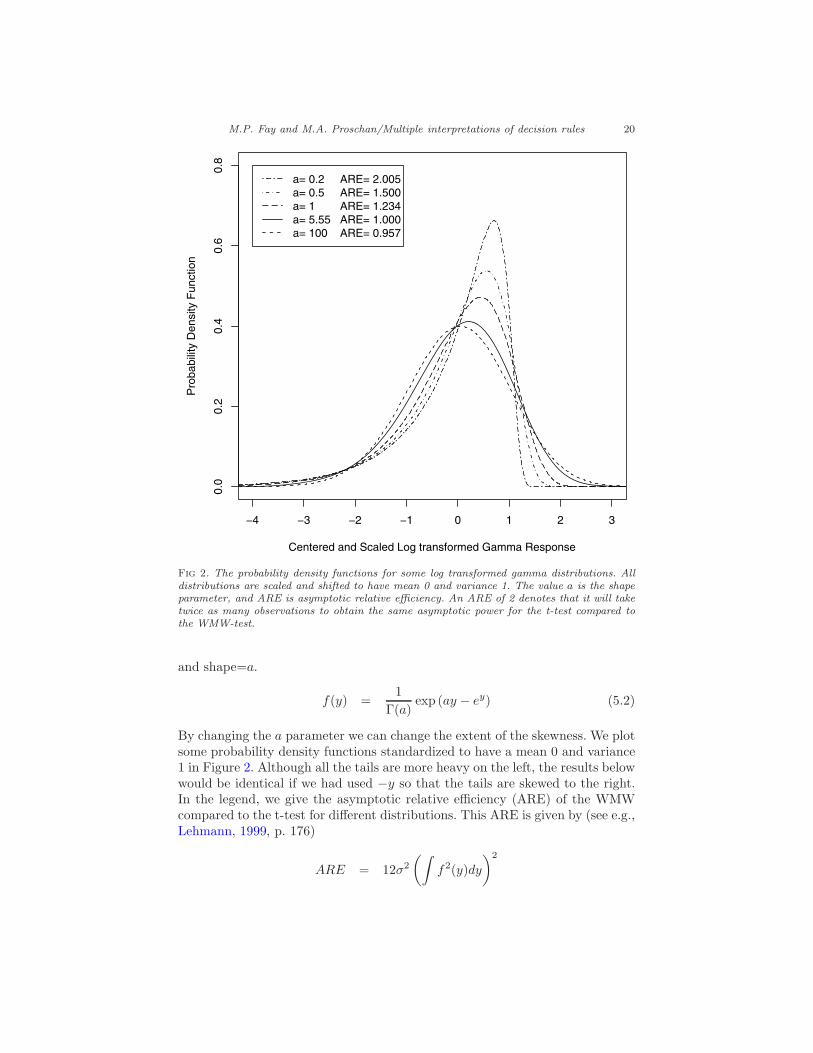
Fig 2. The probability density functions for some log transformed gamma distributions. Alldistributions are scaled and shifted to have mean 0 and variance 1. The value a is the shapeparameter, and ARE is asymptotic relative efficiency. An ARE of 2 denotes that it will taketwice as many observations to obtain the same asymptotic power for the t-test compared tothe WMW-test.

and shape=a.

f(y) =1

Γ(a)exp (ay − ey) (5.2)

By changing the a parameter we can change the extent of the skewness. We plotsome probability density functions standardized to have a mean 0 and variance1 in Figure 2. Although all the tails are more heavy on the left, the results belowwould be identical if we had used −y so that the tails are skewed to the right.In the legend, we give the asymptotic relative efficiency (ARE) of the WMWcompared to the t-test for different distributions. This ARE is given by (see e.g.,Lehmann, 1999, p. 176)

ARE = 12σ2

(∫

f2(y)dy

)2


a

Asym

pto

tic R

ela

tive

Eff

icie

ncy (

WM

W t

o t

)

1.0

1.5

2.0

2.5

3.0

0.001 0.01 0.1 1 10 100

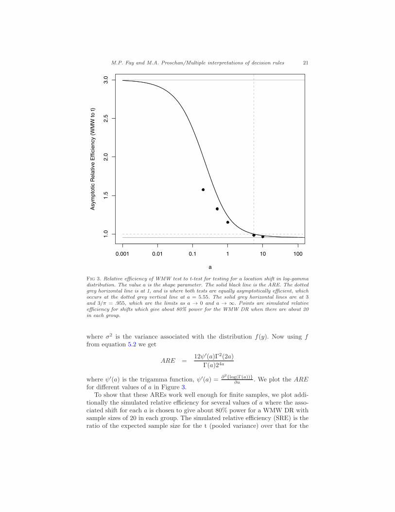
Fig 3. Relative efficiency of WMW test to t-test for testing for a location shift in log-gammadistribution. The value a is the shape parameter. The solid black line is the ARE. The dottedgrey horizontal line is at 1, and is where both tests are equally asymptotically efficient, whichoccurs at the dotted grey vertical line at a = 5.55. The solid grey horizontal lines are at 3and 3/π = .955, which are the limits as a → 0 and a → ∞. Points are simulated relativeefficiency for shifts which give about 80% power for the WMW DR when there are about 20in each group.

where σ2 is the variance associated with the distribution f(y). Now using ffrom equation 5.2 we get

ARE =12ψ′(a)Γ2(2a)

Γ(a)24a

where ψ′(a) is the trigamma function, ψ′(a) = ∂2{log(Γ(a))}∂a . We plot the ARE

for different values of a in Figure 3.To show that these AREs work well enough for finite samples, we plot addi-

tionally the simulated relative efficiency for several values of a where the asso-ciated shift for each a is chosen to give about 80% power for a WMW DR withsample sizes of 20 in each group. The simulated relative efficiency (SRE) is theratio of the expected sample size for the t (pooled variance) over that for the


exact WMW, where the expected sample size for each test randomizes betweenthe sample size, say n, that gives power higher than .80 and n − 1 that givespower lower than .80 such that the expected power is .80 (see Lehmann, 1999,p. 178). The powers are estimated by a local linear kernel smoother on a seriesof simulations at different sample sizes (with up to 105 replications for samplesizes close to the power of .80).

Note that from Figure 2 the distribution where the ARE=1 looks almostsymmetric. Thus, histograms for moderate sample sizes that look symmetricmay still have some small indiscernible asymmetry which causes the WMW DRto be more powerful.

Now suppose the underlying data have a t-distribution, which highlights theheavy tailed case. The ARE of the WMW test to the t-test when the distributionis t with d degrees of freedom (d > 2) is

ARE =12Γ4

(

d+12

)

Γ2(

2d+12

)

π(d− 2)Γ4(

d2

)

Γ2 (d+ 1)(5.3)

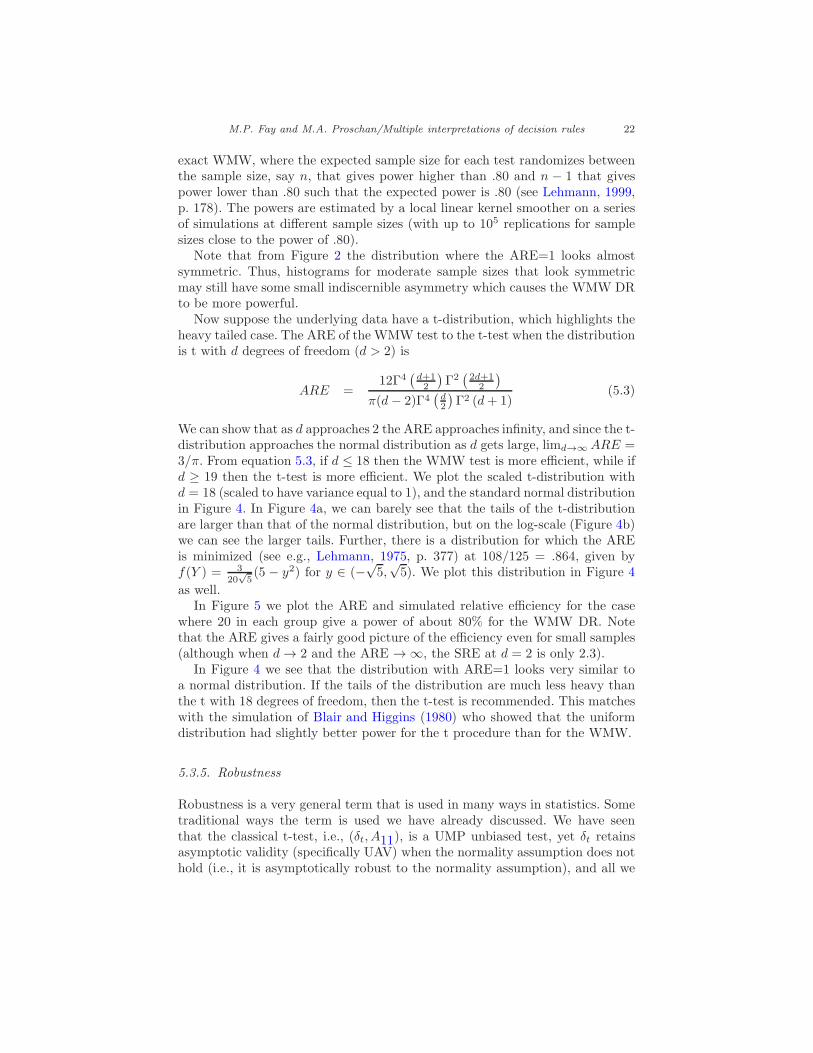
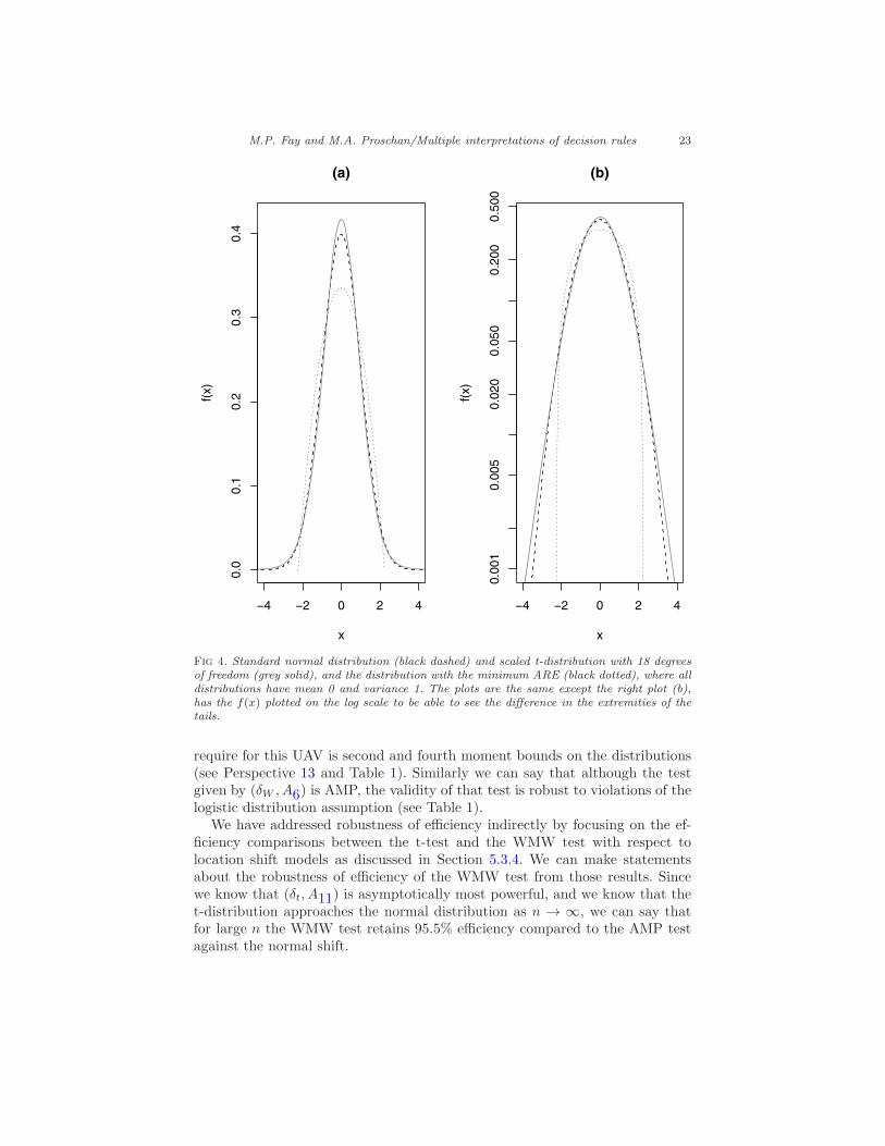
We can show that as d approaches 2 the ARE approaches infinity, and since the t-distribution approaches the normal distribution as d gets large, limd→∞ARE =3/π. From equation 5.3, if d ≤ 18 then the WMW test is more efficient, while ifd ≥ 19 then the t-test is more efficient. We plot the scaled t-distribution withd = 18 (scaled to have variance equal to 1), and the standard normal distributionin Figure 4. In Figure 4a, we can barely see that the tails of the t-distributionare larger than that of the normal distribution, but on the log-scale (Figure 4b)we can see the larger tails. Further, there is a distribution for which the AREis minimized (see e.g., Lehmann, 1975, p. 377) at 108/125 = .864, given byf(Y ) = 3

20√5(5 − y2) for y ∈ (−

√5,√5). We plot this distribution in Figure 4

as well.In Figure 5 we plot the ARE and simulated relative efficiency for the case

where 20 in each group give a power of about 80% for the WMW DR. Notethat the ARE gives a fairly good picture of the efficiency even for small samples(although when d→ 2 and the ARE → ∞, the SRE at d = 2 is only 2.3).

In Figure 4 we see that the distribution with ARE=1 looks very similar toa normal distribution. If the tails of the distribution are much less heavy thanthe t with 18 degrees of freedom, then the t-test is recommended. This matcheswith the simulation of Blair and Higgins (1980) who showed that the uniformdistribution had slightly better power for the t procedure than for the WMW.

5.3.5. Robustness

Robustness is a very general term that is used in many ways in statistics. Sometraditional ways the term is used we have already discussed. We have seenthat the classical t-test, i.e., (δt, A11), is a UMP unbiased test, yet δt retainsasymptotic validity (specifically UAV) when the normality assumption does nothold (i.e., it is asymptotically robust to the normality assumption), and all we


−4 −2 0 2 4

0.0

0.1

0.2

0.3

0.4

(a)

x

f(x)

−4 −2 0 2 4

0.0

01

0.0

05

0.0

20

0.0

50

0.2

00

0.5

00

(b)

x

f(x)

Fig 4. Standard normal distribution (black dashed) and scaled t-distribution with 18 degreesof freedom (grey solid), and the distribution with the minimum ARE (black dotted), where alldistributions have mean 0 and variance 1. The plots are the same except the right plot (b),has the f(x) plotted on the log scale to be able to see the difference in the extremities of thetails.

require for this UAV is second and fourth moment bounds on the distributions(see Perspective 13 and Table 1). Similarly we can say that although the testgiven by (δW , A6) is AMP, the validity of that test is robust to violations of thelogistic distribution assumption (see Table 1).

We have addressed robustness of efficiency indirectly by focusing on the ef-ficiency comparisons between the t-test and the WMW test with respect tolocation shift models as discussed in Section 5.3.4. We can make statementsabout the robustness of efficiency of the WMW test from those results. Sincewe know that (δt, A11) is asymptotically most powerful, and we know that thet-distribution approaches the normal distribution as n → ∞, we can say thatfor large n the WMW test retains 95.5% efficiency compared to the AMP testagainst the normal shift.


0 10 20 30 40

1.0

1.5

2.0

2.5

3.0

3.5

4.0

Degrees of Freedom

Asym

pto

tic R

ela

tive

Eff

icie

ncy (

WM

W t

o t

)

Fig 5. Relative efficiency of WMW test to t-test for testing for location shift in t-distributions.The dotted grey horizontal line is at 1, and is where both tests are equally asymptoticallyefficient, which occurs at the dotted grey vertical line at 18.76. The solid grey lines denotelimits, the vertical line shows ARE goes to infinity at df = 2, the horizontal line shows AREgoes to 3/π = .955 as df → ∞. Points are simulated relative efficiency for shifts which giveabout 80% power for the WMW DR when there are about 20 in each group.

Consider another type of robustness. Instead of wishing to make inferencesabout the entire distribution of the data, we may wish to make inferences aboutthe bulk of the data. For example, consider a contamination model where thedistribution F (G) may be written in terms of a primary distribution, Fp (Gp)and an outlier distribution, Fo (Go) with ǫf (ǫg) of the data following the outlierdistribution. In other words,

F = (1− ǫf )Fp + ǫfFo

and (5.4)

G = (1− ǫg)Gp + ǫgGo

In this setup, we want to make inferences about Fp and Gp, not about F andG, and the distributions Fo and Go represent gross errors that we do not wish


to overly influence our results. In this setup, the WMW decision rule outper-forms the t-test in terms of robustness of efficiency. We can perform a simplesimulation to demonstrate this point. Consider X1, . . . , X100 ∼ N(0, 1) andY1, . . . , Y99 ∼ N(1, 1) and Y100 = 1000 is an outlier caused by perhaps an er-ror in data collection. When we simulate the scenario excluding Y100, then allp-values for δt and δtW are less than 5 ×10−6 and all for δW are less than 3×10−5, while if we include Y100 we get simulated p-values for δt and δtW be-tween 0.26 and 0.29 and p-values for δW between 10−15 and 10−4. Clearly theWMW decision rule has much better power to detect differences between Fp

and Gp in the presence of the outlier. Here we see that only one very gross errorin the data may totally “break down” the power of the t-test, even when theoutlier is in the direction away from the null hypothesis. A formal statement ofthis property is given in He, Simpson and Portnoy (1990).

There is an extensive literature on robust methods in which many more as-pects of robustness are described in very precise mathematics, and althoughnot a focus, robustness for testing is addressed within this literature (see e.g.,Hampel, Ronchetti, Rousseeuw and Stahel, 1986; Huber and Ronchetti, 2009;Jureckova and Sen, 1996). Besides the power breakdown function previouslymentioned, an important theoretical idea for limiting the influence of outliers isto find the maximin test, the test which maximizes the minimum power afterdefining the null and alternative hypotheses as neighborhoods around simple hy-potheses (e.g., using equation 5.4 with Fp andGp representing two distinct singledistributions). Huber (1965) showed that maximin tests (also called minimaxtests) are censored likelihood ratio-type tests (see also Lehmann and Romano,2005, Section 8.3, or Huber and Ronchetti, 2009, Chapter 10). The problemwith this framework is that it is not too convenient for composite hypotheses(Jureckova and Sen, 1996, p. 407). An alternative more general framework is towork out asymptotic robustness based on the influence function (see Huber andRonchetti, 2009, Chapter 13). A thorough review of those robust methods andrelated methods and properties are beyond the scope of this paper.

5.3.6. Recommendations on choosing decision rules

The choice of a decision rule for an application should be based on knowledge ofthe application, and ideally should be done before looking at the data to avoidthe appearance of choosing the DR to give the lowest p-value. To keep this sec-tion short, we focus on choosing primarily between δt (or δtW ) and δW , althoughfor any particular application one of the other tests presented in Table 1 maybe appropriate. When using the less well known or more complicated DRs, oneshould decide whether their added complexity is worth the gains in robustnessof validity or some other property.

The choice between t- and WMW DRs should not be based on a test of nor-mality. We have seen that under quite general conditions the t-test decision rulesare asymptotically valid (see Table 1), so even if we reject the normality assump-tion, we may be justified in using a t-test decision rule. Further, when the data


are close to normal or the sample size is small it may be very difficult to rejectnormality. Hampel et al. (1986, p.23), reviewed some research on high-qualitydata and the departures from normality of that data. They found that usuallythe tails of the distribution are larger than the normal tails and t-distributionswith degrees of freedom from 3 to 10 often fit real data better than the normaldistribution. In light of the difficulty in distinguishing between normality andthose t-distributions with moderate sample sizes, and in light of the relative ef-ficiency results that showed that the WMW is asymptotically more powerful fort-distributions with degrees of freedom less than 18 (see Section 5.3.4), it seemsthat in general the WMW test will often be asymptotically more powerful thanthe t-test for real high quality data. Additionally, the WMW DR has betterpower properties than the classical t-test when the data are contaminated bygross errors (see Section 5.3.5).

In a similar vein to the recommendation not to test for normality, it is notrecommended to use a test of homogeneity of variances to decide between theclassical (pooled variance) t-test DR (δt) and Welch’s DR (δtW ), since thisprocedure can inflate the type I errors (Moser, Stevens and Watts, 1989).

One case where a t-test procedure may be clearly preferred over the WMWDR is when there are too few observations to produce significance for the WMWDR (see Section 5.3.3). Also, if there are differences in variance, then δtW (orsome of the other decision rules, see Table 1) may be used while δW is not valid.In general, whenever the difference in means is desired for interpretation of thedata, then the t-tests are preferred. Nonetheless, if there is a small possibilityof gross errors in the data (see Section 5.3.5), then there may be better robustestimators of the difference in means which will have better properties (seeReferences in Section 5.3.5).

6. Other examples and uses of MPDRs

In Section 5 we went into much detail on how some common tests may beviewed under different perspectives. In this section, we present without detailstwo examples that show different ways that the MPDR framework can be useful.

6.1. Comparing decision rules: Tests for interval censored data

Another use of the MPDR outlook is to compare DRs developed under differentassumptions. Sun (1996) developed a test for interval censored data under theassumption of discrete failure times. In the discussion of that paper, Sun statesthat his test “is for the situation in which the underlying variable is discrete”and “if the underlying variable is continuous and one can assume proportionalhazards model, one could use Finkelstein’s [1986] score test”. Although there canbe subtle issues in differentiating between continuous and discrete models espe-cially as applied to censored data (see e.g., Andersen, Borgan, Gill and Keiding,1993, Section IV.1.5), in this case Sun’s (1996) test can be applied if the un-derlying variable is continuous. If we look at Sun’s (1996) DR as a MPDR then


this extends the usefulness and applicability of his test, since it can be appliedto both continuous and discrete data. In fact, under the MPDR outlook Finkel-stein’s (1986) test can be applied to discrete data as well. See Fay (1999) fordetails.

6.2. Interpreting rejection: Genetic tests of neutrality

In the examples of Section 5, the MPDR outlook was helpful in interpreting thescope of the decision. Some perspectives provide a fairly narrow scope with per-haps some optimal property (e.g., t-test of difference in normal means with thesame variances is uniformly most powerful unbiased), while other perspectivesprovide a much broader scope for interpreting similar effects (e.g., the differencein means from the t-test can be asymptotically interpreted as a shift in locationfor any distribution with finite variance). In this section, we provide an exam-ple where the different perspectives do not just provide a difference betweena broad or narrow scope of the same general tendency, but the different per-spectives highlight totally different effects. In other words, from one perspectiverejecting the null hypothesis means one thing, and from another perspectiverejecting the null hypothesis means something else entirely.

The example is a test of genetic neutrality (Tajima’s [1989] D statistic), andthe original perspective on rejection is that evolution of the population has notbeen neutral (e.g., natural selection has taken place). This perspective requiresmany assumptions. Before mentioning these we first briefly describe the DR.

The data for this problem are n sequences of DNA, where each sequence isfrom a different member of a population of n individuals from the same species.The sequences have been aligned so that each sequence is an ordered list of wletters, where each letter represents one of the four nucleotides of the geneticcode (A,T,C, and G). We call each position in the list, a site. Let S be the

number of sites where not all n sequences are equal to the same letter. Let k bethe average number of pairwise differences between the n sequences. Tajima’sD statistic is

D =k − S

a1√

V

where a1 =∑n−1

i=11i , and V is an estimate of the variance of k − S

a1

which isa function of S and some constants which are functions of n only (see Tajima,1989, equation 38). We reject if D is extreme compared to a generalized betadistribution over the range Dmin to Dmax with mean equal to 0 and variance1, and both range parameters are also functions of n only (see Tajima, 1989).

To create a probability model for D Tajima assumed (under the null hypoth-esis) that:

1. there is no selection (i.e., there is genetic neutrality),2. the population size is not changing over time,3. there is random mating in the population,4. the species is diploid (has two copies of the genetic material),


5. there is no recombination (i.e., a parent passes along either his/her mother’sor his/her father’s genetic material in its entirety instead of picking outsome from the mother and some from the father),

6. any new mutation happens at a new site where no other mutations havehappened,

7. the mutation rate is constant over time.

If all the assumptions hold then Tajima’s D has expectation 0 and the associatedDR is an approximately valid test. The problem is that when we observe anextreme value of D, then it could be either due to (1) chance (but this is unlikelybecause it is an extreme value), (2) selection has taken place in that population(i.e., assumption 1 is not true), or (3) one of the other assumptions may notbe true. This interpretation may seem obvious, but unfortunately, according toEwens (2004), p. 348, the theory related to tests of genetic neutrality is oftenapplied “without any substantial assessment of whether [the assumptions] arereasonable for the case at hand”.

The MPDR framework applied to this problem could define the same nullhypothesis as listed above, but have a different alternative hypothesis for eachperspective according to whether one of the assumptions does not hold. Forintuition into the following, recall that D will be negative if each site on averagehas a lower frequency of pairwise nucleotide differences than would be expected.Now consider alternatives where one and only one of the assumptions of the nullis false.

Selection: If Assumption 1 is false, then the associated alternative creates aperspective that is Tajima’s original one, and that is why the test is calleda test of genetic neutrality. When we reject the null hypothesis, then this isseen as implying that there is selection (i.e., there is not genetic neutrality).Specifically, if there has recently been an advantageous mutation suchthat variability is severely decreased in the population, this is a selectivesweep and the expectation of D would be negative. Conversely, if there isbalancing selection, then the expectation of D would be positive (see e.g.,Durrett, 2002).

Non-constant Population Size: Consider when Assumption 2 is false underthe alternative.

Growth of Population: If the population is growing exponentially thenwe would expect D to be negative (see e.g., Durrett, 2002, p. 154).

Recent Bottleneck: A related alternative view is that the genetic vari-ation in the population happened within a fairly large population,but then the population size was suddenly reduced dramatically andthe small remaining population grew into a larger one again. Thisis known as bottle-necking (see e.g., Winter, Hickey and Fletcher,2002). Tajima (1989) warned that rejection of the null hypothesiscould be caused by recent bottlenecking, and Simonsen, Churchilland Aquadro (1995) showed that Tajima’s D has reasonable powerto reject under the alternative hypothesis of a recent bottleneck.


Random Mating: Consider the alternative where Assumption 3 is false. Ifthe mating is more common (but still random) within subgroups, thenthis can lead to positive expected values of D (see e.g., Durrett, 2002, p.154, Section 2.3).

These results for Tajima’s D are now ‘well known’, and a user of the methodshould be aware of all the possible alternative interpretations (different perspec-tives) when the null hypothesis is rejected. As with other MPDRs the p-valueis calculated the same way, but the interpretation has very real differences de-pending on the perspective. But unlike the previous examples of Section 5 and6.1, the different interpretations are not just an expansion or shrinkage of scopeof applicability, but they describe qualitatively different directions for lookingat rejection of the null.

7. Discussion

We have described a framework where one DR may be interpreted under manydifferent sets of assumptions or perspectives. We conclude by reemphasizing twomajor points highlighted by the MPDR framework:

• Do not necessarily disregard results of a decision rule becauseit is obviously invalid from one perspective. Perhaps it is valid orapproximately valid from a different perspective. For example, consider ahypothesis test comparing two HIV vaccines, where the response is HIVviral load in the blood one year after vaccination. Even if both groups havemedian HIV viral loads of zero even under the alternative (which is verylikely), invalidating the location shift perspective and all more restrictiveperspectives than that (see Figure 1), that does not mean that a WMWDR cannot be applied under a different perspective (e.g., Perspective 3).As another example, suppose that a large clinical trial shows a significantdifference in means by t-test but the test of normality determines thedata are significantly non-normal. Then the t-test p-value can still beused under the general location shift perspective instead of under thenormal shift perspective. Finally, consider the tests for interval censoreddata developed for continuous data which could be shown to be valid fordiscrete data as well (see Section 6.1).

• Be careful of making conclusions by assumption. In Section 6.2 weshowed how the rejection of a genetic test of neutrality could be interpretedmany different ways depending on the assumptions made. Every time agenetic test of neutrality is used, all the different perspectives (sets of as-sumptions) should be kept in mind, since focusing on only one perspectivecould lead to the totally wrong interpretation of the decision rule.

Therefore, the fact that a decision rule can have multiple perspectives can beeither good or bad for clarification of a scientific theory; the MPDR may helpsupport the theory by offering multiple statistical formulations consistent with


it, or the MPDR may highlight statistical formulations that may be consistentwith alternative theories as well.

Appendix A: Nonparametric Behrens-Fisher decision rule ofBrunner and Munzel

Let R1, . . . , Rn be the mid-ranks of the Yi values regardless of Zi value, andlet W1, . . . ,Wn be the within-group mid-ranks (e.g., if there are no ties andWi = w and Zi = 1 then Yi is the wth largest of the responses with Zi = 1).Let R1 = 1

n1

∑ni=1 ZiRi and R0 = 1

n0

∑ni=1(1 − Zi)Ri, and

τ21 =1

n20(n1 − 1)

n∑

i=1

Zi

(

Ri −Wi − R1 +n1 + 1

2

)2

τ20 =1

n21(n0 − 1)

n∑

i=1

(1− Zi)

(

Ri −Wi − R0 +n0 + 1

2

)2

.

More intuitively, we can write τ21 and τ20 as

τ21 =1

n1 − 1

n∑

i=1

Zi

(

G(Yi)− G)2

τ20 =1

n0 − 1

n∑

i=1

(1− Zi)(

F (Yi)− F)2

where F (t) = n−11

∑ni=1 Zi

{

I(Yi < t) + 12I(Yi = t)

}

and F = n−10

∑ni=1(1 −

Zi)F (Yi), and similarly for G and G. Then, let

VJ =

√

τ20n0

+τ21n1

TNBF =n−1

(

R1 − R0

)

√VJ

=φ(F , G)− 1

2√VJ

.

When there is no overlap between the two groups, then τ0 = τ1 = 0 and VJ = 0;in this case Neubert and Brunner (2007), p. 5197, suggest setting VJ equal to thelowest possible non-zero value: 1√

2n2

0n2

1

. We reject when |TNBF | > t−1dB

(1−α/2)

where dB is given by dW of equation 5.1 except that τ20 and τ21 replace σ20 and σ2

1 .

Appendix B: Counterexample to uniform control of error rate forthe t-test

Let Y1, . . . , Yn be iid Bernoulli random variables with parameter pn = ln(2)/n.Suppose that the two groups have equal numbers so that n0 = n1 = n/2. Let


S1 =∑n

i=1 ZiYi and S0 =∑n

i=1(1− Zi)Yi. Then

Tt(X) =S1 − S0

√

nn−2

(

S1 − 2S2

1

n + S0 − 2S2

0

n

)

.

When S1 ≥ 1 and S0 = 0 then

Tt(X) =S1

√

nn−2

S1(n−2S1)n

≥ S1√

nn−2

S1(n−2)n

=√

S1 ≥ 1

Now suppose that α = .16 one-sided. If n ≥ 100 then t−1n−2(.84) ≥ .9995 and we

would reject whenever S1 ≥ 1 and S0 = 0, which occurs with probability

Pr [S1 ≥ 1 and S0 = 0] = (1− Pr[S1 = 0])Pr[S0 = 0] = (1− qn1)qn0

≈ 0.25

where qn =(

1− ln(2)n

)nand the approximation uses limn→∞ qn = exp(− ln(2)) =

12 ; for n = 100 we get q50(1−q50) = 0.249994 and for n > 100 the approximationgets closer to .25. Therefore, for this sequence of distributions, with n > 100 thetype I error rate is 0.249 or more instead of the intended 0.16.

Appendix C: Sufficient conditions for uniform control for the t-test

The test δt is UAV if we impose certain conditions on the common distributionfunction F . For example, for 0 < B < ∞ and ǫ > 0, consider the class ΨB,ǫ ofdistribution functions such that V ar(Y ) ≥ ǫ and E(Y 4) ≤ B. We will show thatfor every sequence of functions Fn ∈ ΨB,ǫ, assuming limn→∞ n0/n = λ0 and0 < λ0 < 1, the type 1 error rate has limit α. We do this in three steps: 1) weuse the Berry-Esseen theorem to show that even though Fn may change withn, the distribution of the z-score associated with the sample mean convergesuniformly to a normal distribution, 2) we show that the same is true of thez-score for the difference of two sample means, and 3) we show that the sameis true for the t-score, which uses the sample variance instead of the populationvariance in the denominator.

Step 1

Consider a sequence of distribution functions Fn ∈ ΨB,ǫ with associated meanand variance equal to µn and σ2

n. In this appendix Yn denotes a random variablefrom Fn and the sample means for each group are µ1n and µ0n. According tothe Berry-Esseen theorem, for any sequence of distribution functions Fn ∈ ΨB,ǫ,

supz

∣

∣

∣

∣

∣

Pr

{

µ1n − µn

σn/√n1

≤ z

}

− Φ(z)

∣

∣

∣

∣

∣

≤ 33

4

E|Yn − µn|3σ3n

√n1

,


for all n. Of course the same is true of the group with Zi = 0 except with n1

replaced by n0, because they have the same distribution. Notice that E|Yn −µn|3 ≤ {E|Yn − µn|4}3/4, and

|Yn − µn|4 ≤ (|Yn|+ |µn|)4 ≤ {2max(|Yn|, |µn|)}4

= 24{max(|Yn|, |µn|)}4 ≤ 24(|Yn|4 + |µn|4)= 16(Y 4

n + |E(Yn)|4) ≤ 16(Y 4n + E(Y 4

n ))

≤ 16(Y 4n +B).

It follows that E|Yn−µn|4 ≤ 16(E(Y 4n )+B) ≤ 32B, so E|Yn−µn|3 ≤ (32B)3/4.

Furthermore, because σ2n ≥ ǫ, the Berry-Esseen bound is no greater than An1

=(33/4)(32B)3/4/{n1ǫ

3}1/2 → 0. The same result holds for the second group.

Step 2

We next show that even though the distribution function Fn may change withn, (µ1n − µ0n)/(σ

2n(1/n1 + 1/n0))

1/2 converges uniformly to a standard normaldistribution. Specifically, we show that

supz

∣

∣

∣

∣

∣

Pr

{

µ1n − µn

σnbn− Yn − µn

σnbn≤ z

}

− Φ(z)

∣

∣

∣

∣

∣

≤ An1+An0

,

where bn = (1/n0 + 1/n1)1/2.

Let λ0n = n0/n and λ1n = 1 − λ0n = n1/n, so that λ1/20n = b−1

n n−1/21 , and

assume that λ0n → λ0 and 0 < λ0 < 1. Let Hn1and Hn0

denote the distribution

functions for Zn1= (µ1n − µn)/(σn/n

1/21 ) and Z ′

n0= (µ0n − µn)/(σn/n

1/20 ),

respectively. Then

Pr(

Zn

√

λ0n − Z ′n

√

λ1n ≤ z)

=

∫ ∞

−∞Hn1

(

z√λ0n

+ u

√

λ1nλ0n

)

dHn0(u)

=

∫ ∞

−∞

{

Φ

(

z√λ0n

+ u

√

λ1nλ0n

)

+Hn

(

z√λ0n

+ u

√

λ1nλ0n

)

−

Φ

(

z√λ0n

+ u

√

λ1nλ0n

)}

dHn0(u)

= Cn +Dn,


where

Cn =

∫ ∞

∞Φ

(

z√λ0n

+ u

√

λ1nλ0n

)

dHn0(u),

and

Dn =

∫ ∞

−∞

{

Hn1

(

z√λ0n

+ u

√

λ1nλ0n

)

− Φ

(

z√λ0n

+ u

√

λ1nλ0n

)}

dHn0(u).

Note that Cn = Pr(V < z√λ0n

+ Z ′n0

√

λ1n

λ0n) = Pr(Z ′

n0> V

√

λ0n

λ1n− z√

λ1n),

where V is independent of Z ′n0

and has a standard normal distribution. We cantherefore rewrite Cn as

Cn =

∫

{

1−Hn0

(

v

√

λ0nλ1n

− z√λ1n

)}

φ(v)dv

=

∫

{

1− Φ

(

v

√

λ0nλ1n

− z√λ1n

)}

φ(v)dv +

∫

{

Φ

(

v

√

λ0nλ1n

− z√λ1n

)

−Hn0

(

v

√

λ0nλ1n

− z√λ1n

)}

φ(v)dv

= Φ(z)−∫

{

Φ

(

v

√

λ0nλ1n

− z√λ1n

)

−Hn0

(

v

√

λ0nλ1n

− z√λ1n

)}

φ(v)dv

To show the last step, notice that if we let V and V ′ be independent standardnormals, then V

√λ0n − V ′√1− λ0n is standard normal, so that

∫

{

1− Φ

(

v

√

λ0nλ1n

− z√λ1n

)}

φ(v)dv = Pr

[

V ′ > V

√

λ0nλ1n

− z√λ1n

]

= Pr[

V√

λ0n − V ′√λ1n ≤ z]

= Φ(z)

Thus,

|Cn − Φ(z)| ≤∫ ∞

−∞

∣

∣

∣Hn0

(

v

√

λ0nλ1n

− z√λ1n

)

− Φ

(

v

√

λ0nλ1n

− z√λ1n

)

∣

∣

∣φ(v)dv

≤∫ ∞

−∞An0

φ(v)dv = An0,

where An0is as specified at the end of step 1. Also,

|Dn| ≤∫ ∞

−∞

∣

∣

∣Hn1

(

v

√

λ0nλ1n

− z√λ1n

)

− Φ

(

v

√

λ0nλ1n

− z√λ1n

)

∣

∣

∣dHn0

(u)

≤∫ ∞

−∞An1

dHn0(u) = An1

.


In summary,

Pr(

Zn

√

λ0n − Z ′n

√

λ1n ≤ z)

= Φ(z) + Cn − Φ(z) +Dn

∣

∣

∣Pr(

Zn

√

λ0n − Z ′n

√

λ1n ≤ z)

− Φ(z)∣

∣

∣≤ |Cn − Φ(z)|+ |Dn|≤ An0

+An1→ 0. (C.1)

Step 3

The next step is to show that the t-statistic, Tt, also converges to a standardnormal distribution. To do so, we will show that σ2

pn/σ2n converges to 1 in

probability, where σ2pn is the pooled variance. Because σ2

n ≥ ǫ, this is equivalentto showing that σ2

np − σ2n → 0 in probability. It is clearly sufficient to show that

this is true of each of the two sample variances, say σ21n and σ2

0n, since σ2pn is

a weighted average of the two sample variances. In the following, we consideronly the group with Zi = 1 so all summations are over {i : Zi = 1}, and furtherlet Yin ∼ Fn for all i.

(n1 − 1)σ2n1

=∑

(Yin − µn + µn − µ1n)2

=∑

(Yin − µn)2 + n1(µn − µn1)

2 + 2(µn − µn1)∑

(Yin − µn)

=∑

(Yin − µn)2 + n1(µn1 − µn)

2 − 2n1(µn1 − µn)2

=∑

(Yin − µn)2 − n1(µn1 − µn)

2.

That is, σ21n = (n1−1)−1

{∑

(Yin − µn)2 − n1(µ1n − µn)

2}

. The proof is slightlyeasier if we replace n1− 1 with n1. Therefore, we show that

∑

(Yin −µn)2/n1−

(µ1n − µn)2 − σ2

n → 0 in probability. Use Markov’s inequality to conclude that(µ1n − µn)

2 converges to 0 in probability: Pr{(µ1n − µn)2 > η} ≤ E(µ1n −

µn)2/η = var(µ1n)/η = σ2

n/(n1η), and σ2n = E(Yn − µn)

2 ≤√

E(Yn − µn)4 ≤√32B (from the calculations in step 1). Thus, (µ1n − µn)

2 → 0 in probability.The only remaining task is to prove that |∑(Yin − µn)

2/n1 − σ2n| converges in

probability to 0. Note that

Pr

(∣

∣

∣

∣

∣

∑

(Yin − µn)2

n1− σ2

n

∣

∣

∣

∣

∣

> η

)

≤ var(

∑

(Yin − µn)2/n1

)

/η2

=var(Yn − µn)

2

n1η2

=E((Yn − µ)4)− {E(Yn − µn)

2}2n1η2

≤ E(|Yn − µ|4)n1η2

≤ 32B

n1η2→ 0.


Appendix D: Justifications for Table 1

D.1. Validity

All the permutation-based DRs (e.g., δW , δNBFp, δtp, and δJ) are valid whenevereach permutation is equally likely under all θ ∈ ΘH . These DRs can be expressedby either permuting the Z values or permuting the Y values; therefore, allperspectives with F = G for all models in the null space, plus Perspective 9(the randomization model) give valid tests.

Under H12 then δt is asymptotically equivalent to δtp, so when δt is not validfor less restrictive hypotheses (e.g., Perspectives 14 and 15, see below), δtp isalso not valid. Since we have assumed F,G ∈ Ψfv for all of Table 1, wheneverδtp is valid then δt is at least PAV.

Since the denominator of TBF can be written as σBF (1/n1 + 1/n0)1/2 with

σ2BF = n−1

(

n0σ21 + n1σ

20

)

, and we see that σ2BF is just a weighted average of the

individual sample variances, then similar methods to Appendix C can be usedto show that the other t-tests (δtW and δtH) are also UAV under Perspective 13.

The δt is valid under Perspective 11 and δtH is valid under Perspective 14(see e.g., Dudewicz and Mishra, 1988, p. 502), so (δtH , A11) is valid. SinceδtW is equivalent to δtH except it has larger degrees of freedom (see e.g.,Dudewicz and Mishra, 1988, p. 502), it is UAV under Perspectives 14 and 11.One can show that (δtW , A11) is not valid for finite samples by simulationfrom standard normal with n1 = 2 and n0 = 30, which gives type I error ofaround 12%.

The rules δNBFaand δNBFp

were shown to be PAV under H10 (see Brunnerand Munzel, 2000 and Neubert and Brunner, 2007 respectively).

For any null where F = G and F ∈ ΨC , any rank test that is PAV and onlydepends on the combined ranks is also UAV. To see that, note that such a DRis invariant to monotone transformations. Thus, if we let Y ∗

in = Fn(Yin) for alli = 1, . . . , n, where Fn is the common distribution function regardless of Zi,then the Y ∗

ins are iid uniforms. The type I error rate of the rank test applied tothe original data is the same as that applied to the uniforms, so the type I errorrate is controlled uniformly over all continuous distributions.

Pratt (1964) showed that under the Perspective 14 (Behrens-Fisher), boththe WMW and the t tests are not valid (not even PAV), so since A14 < A15and and A14 < A10, both those DRs are not valid under Perspectives 15 and10. However, note that when n1 = n0 then Tt = TBF , and (δt, A14) is UAV.We have previously shown in Section 5.2.2 that Perspective 15 is invalid forany DR which has power > α for some P ∈ K15. For Perspective 10 we canshow the two simple discrete distributions with three values at (−1, 0, 2) andprobability density functions at those three points as (.01, .98, .01) (associatedwith F ) and (.48, .02, .48) (associated with G) are in H10 but are not valid forδtW , δtH or δBFp.


D.2. Consistency

The consistency of δW was shown for Perspective 3 by Lehmann (1951) andPutter (1955) expanded this result showing consistency for discrete distribu-tions. We can use the relationship among the assumptions (see Figure 1) toshow consistency for most of Table 1. Brunner and Munzel (2000) showed theasymptotic normality of TNBF whenever φ(F,G) = 1/2 and V ar(F (YG)) > 0and V ar(G(YF )) > 0, and it is straightforward to extend this to show theasymptotic normality of

TNBF (φ) =φ(F , G)− φ(F,G)

√

τ2

0

n0

+τ2

1

n1

,

even when φ(F,G) 6= 1/2. Thus, δNBFa is consistent for Perspective 10 and allmore restrictive assumptions. Neubert and Brunner (2007) showed the asymp-totic normality of the permutation version TNBF (φ) and hence δNBFp is con-sistent for the same perspectives as δNBFa. For all three rank DRs (δW , δNBFa

and δNBFp), the associated tests are not consistent when there are alternativeswhich include probability models with φ(F,G) = 1/2.

The consistency of δt under K12 is shown in e.g., Lehmann and Romano(2005), p. 466, and it is straightforward to extend this to δtW and δtH . Thus, forall more restrictive assumptions those tests are also consistent. Similar methodsanalogously show that both δtW and δtH are consistent for K14. For alternativesthat contain probability models with µ0 = µ1, all the t-tests are not consistent.

UnderK11 then δt is asymptotically equivalent to δtp (Lehmann and Romano,2005, p. 683, problem 15.10); therefore δtp is consistent. Janssen (1997), The-orem 2.2, showed the consistency of δtBFp as long as µ0 6= µ1 under a lessrestrictive assumptions than A14 which include A6 and A7. The DRs δtp andδBFp are consistent whenever respectively, δp and δW are consistent assumingfinite variances (see van der Vaart, 1998, p. 188).

References

Andersen, P.K., Borgan, O, Gill, R.D., and Keiding, N. (1993). Sta-tistical Models Based on Counting Processes Springer-Verlag: New York.MR1198884

Berger, R.L. and Boos, D.D. (1994). P values maximized over a confidenceset for the nuisance parameter. Journal of the American Statistical Associa-tion 89 1012–1016. MR1294746

Blair, R. C. and Higgins, J.J. (1980). A comparison of the power ofWilcoxon’s rank-sum statistic to that of Student’s t statistic under variousnonnormal distributions. Journal of Educational Statistics 5 309–334.

Box, G.E.P., Hunter, J.S., and Hunter, W.G. (2005). Statistics for Ex-perimenters: Design, Innovation, and Discovery, second edition. Wiley: NewYork. MR2140250

http://www.ams.org/mathscinet-getitem?mr=1198884




Brunner, E. and Munzel, U. (2000). The Nonparametric Behrens-FisherProblem: Asymptotic Theory and a Small-Sample Approximation. Biometri-cal Journal 42 17–25. MR1744561

Cao, H. (2007). Moderate deviations for two sample t-statistics. ESAIM: Prob-ability and Statistics 11 264–271. MR2320820

Cox, D.R. and Hinkley, D.V. (1974). Theoretical Statistics Chapman andHall: London. MR0370837

Dowdy, S., Wearden, S., and Chilko, D. (2004). Statistics for Research,third edition Wiley: New York.

Dudewicz, E.J. and Mishra, S.N. (1988). Modern Mathematical StatisticsWiley: New York. MR0920168

Durrett, R. (2002). Probability models for DNA sequence evolution. Springer:New York. MR1903526

Edgington,E.S. (1995). Randomization Tests, third edition. Marcel Dekker,Inc.: New York.

Ewens, W.J. (2004). Mathematical Population Genetics. I. Theoretical Intro-duction, second edition Springer: New York. MR2026891

Fay, M.P. (1999). Comparing several score tests for interval censored data.Statistics in Medicine 18 273–285 (Correction: 1999; 2681).

Finkelstein, D.M. (1986). A proportional hazards model for interval-censoredfailure time data. Biometrics 42 845–854. MR0872963

Hajek, J. and Sidak, Z. (1967). Theory of Rank Tests Academic Press: NewYork.

Hampel, F.R., Ronchetti, E.M., Rousseeuw, P.J., and Stahel, W.A.

(1986). Robust Statistics: The Approach Based on Influence Functions Wiley:New York. MR0829458

He, X., Simpson, D.G., and Portnoy, S.L. (1990). Breakdown robust-ness of tests. Journal of the American Statistical Association 85 446–452.MR1141746

Hennekens, C.H., Eberlein, K.A., for the Physicians’ Health Study

Research Group. (1985). A randomized trial of aspirin and β-caroteneamong U.S. physicians. Preventive Medicine 14 165–168.

Hettmansperger, T.P. (1984). Statistical Inference Based on Ranks. KriegerPublishing Company: Malabar, Florida. MR0758442

Hodges, J.L. and Lehmann, E.L. (1963). Estimates of Location Based onRank Tests. Annals of Mathematical Statistics 34 598–611. MR0152070

Huber, P.J. (1965). A robust version of the probability ratio test. Annals ofMathematical Statistics 36 1753–1758. MR0185747

Huber, P.J., and Ronchetti, E.M. (2009). Robust Statistics, second editionWiley: New York. MR2488795

Janssen, A. (1997). Studentized permutation tests for non-i.i.d. hypotheses onthe generalized Behrens-Fisher problem. Statistics and Probability Letters 369–21. MR1491070

Janssen, A. (1999). Testing nonparametric statistical functionals with appli-cations to rank tests. Journal of Statistical Planning and Inference 81 71–93.MR1718393

















Jureckova, J. and Sen, P.K. (1996). Robust Statistical Procedures: Asymp-totics and Interrelations Wiley: New York. MR1387346

Kempthorne, O. and Doerfler, T.E. (1969). The behaviour of some sig-nificance tests under experimental randomization. Biometrika 56 231–248.MR0254965

Lehmann, E.L. (1951). Consistency and unbiasedness of certain nonparametrictests. Annals of Mathematical Statistics 22 165–179. MR0040632

Lehmann, E.L. (1975). Nonparametrics: Statistical Methods Based on RanksHolden-Day, Inc.: Oakland, CA. MR0395032

Lehmann, E.L. (1997). Review of Error and the Growth of ExperimentalKnowledge by D.G. Mayo. Journal of the American Statistical Association92 789.

Lehmann, E.L. (1999). Elements of Large-Sample Theory Springer: New York.MR1663158

Lehmann, E.L. and Romano, J.P. (2005). Testing Statistical Hypotheses,third edition Springer, New York. MR2135927

Ludbrook, J. and Dudley, H. (1998). Why permutation tests are superiorto t and F tests in biomedical research. American Statistician 52 127–132.

Mallows, C.L. (2000). Letter to the Editor in Response to Ludbrook andDudley(1998. 54 86–87.

Mann, H.B. and Whitney, D.R. (1947). On a Test of Whether One of TwoRandom Variables is Stochastically Larger Than the Other. Annals of Math-ematical Statistics 18 50–60. MR0022058

Mayo, D.G. (1996). Error and the Growth of Experimental Knowledge Univer-sity of Chicago Press, Chicago.

Mayo, D.G. (2003). Comment on Could Fisher, Jefferys and Neyman HaveAgreed on Testing. by J.O. Berger. Statistical Science 18 19–24. MR1997064

Mayo, D.G. and Spanos, A. (2004). Methodology in Practice: Statistical Mis-specification Testing. Philosophy of Science 71 1007–1025. MR2133711

Mayo, D.G. and Spanos, A. (2006). Severe Testing as a Basic Concept in aNeyman-Pearson Philosophy of Induction. 57 323–357. MR2249183

McCullagh, P. (1980). Regression models for ordinal data. (with discussion)Journal of the Royal Statistical Society, series B 42 109–142. MR0583347

McDermott, M.P. and Wang, Y. (1999). Comment on “The emperor’s newtests” by Perlman and Wu Statistical Science 14 374–377.

Mee, R.W. (1990). Confidence intervals for probabilities and tolerance regionsbased on a generalization of the Mann-Whitney statistic. Journal of the Amer-ican Statistical Association. 85 793–800. MR1138359

Mehta, C.R., Patel, N.R., and Tsiatis, A.A. (1984). Exact significancetesting to establish treatment equivalence with ordered categorical data. Bio-metrics 40 819–825. MR0775388

Moser, B.K., Stevens, G.R., and Watts, C.L. (1989). The two-sample ttest versus Satterhwaite’s approximate F test. Communications in Statistics:Theory and Methods 18 3963–3975. MR1058922
















Neubert, K. and Brunner, E. (2007). A Studentized permutation test for thenon-parametric Behrens-Fisher problem. Computational Statistics and DataAnalysis 51 5192–5204. MR2370717

Perlman, M. and Wu, L. (1999). The emperor’s new tests (with discussion).Statistical Science 14, 355–381. MR1765215

Pratt, J.W. (1964). Robustness of some procedures for the two-sample loca-tion problem. Journal of the American Statistical Association 59 665–680.MR0166871

Putter, J. (1955). The treatment of ties in some nonparametric tests. Annalsof Mathematical Statistics 26 368–386. MR0070923

Proschan, M. and Follmann, D. (2008). Cluster without fluster: the effectof correlated outcomes on inference in randomized clinical trials. Statistics inMedicine DOI 10.1002/sim.2977. MR2420113

Sawilowsky, S.S. andBlair, R.C. (1992). A more realistic look at the robust-ness and type II error properties of the t test to departures from populationnormality. Psychological Bulletin 111 (2) 352–360.

Sen, P.K. (1967). A note on asymptotically distribution-free confidence boundsfor Pr{Y < X} based on two independent samples. Sankhya, Ser. A, 29 (Pt.1) 95–102. MR0226772

Simonsen, K.L., Churchill, G.A., and Aquadro, C.F. (1995). Propertiesof statistical tests of neutrality for DNA polymorphism data. Genetics 141413–429.

Sterring Committee of the Physicians’ Health Study Research

Group (1988). Preliminary Report: Findings from the Aspirin Componentof the Ongoing Physicians’ Health Study. New England Journal of Medicine318 262–264.

Sterring Committee of the Physicians’ Health Study Research

Group (1989). Final Report on the Aspirin Component of the Ongoing Physi-cians’ Health Study. New England Journal of Medicine 321 129–135.

Sun, J. (1996). A non-parametric test for interval-censored failure time datawith applications to AIDS studies. Statistics in Medicine, 15, 1387–1395.

Tajima, F. (1989). Statistical method for testing the neutral mutation hypoth-esis by DNA polymorphism. Genetics 123 585–595.

van der Vaart, A.W. (1998). Asymptotic Statistics Cambridge UniversityPress, Cambridge. MR1652247

Wilcoxon, F. (1945). Individual comparisons by Ranking Methods. BiometricsBulletin 1 80–83.

Winter, P.C., Hickey, G.I., and Fletcher, H.L. (2002). Instant Notes:Genetics, second edition. Bios Scientific Publishers: Oxford.

Whitt, W. (1988). Stochastic Ordering. in Encyclopedia of Statistics Vol. 8,S. Kotz and N.L. Johnson (editors). Wiley: New York.








wilcoxon-mann-whitneyor t-test? …healy.econ.ohio-state.edu/fayproschan.pdfstatistics surveys vol....

Documents