i

Wien-Bridge Theremin

Joseph Ballerini

Matthew Newberg

Jason Wright

ECE 4530 – Final Project

Fall 2011

ii

Abstract

A theremin is an early electronic musical instrument invented by Russian inventor Léon Theremin in 1928. It is unique among musical instruments because it is played without any physical contact between performer and instrument – rather, the performer moves his or her hands in various patterns next to one or more antennas or metal plates to change the volume and/or frequency of the output signal. Most commercially available theremins cost upwards of $400, in part due to high production costs for many specialty components in most designs. We chose to design a Wien bridge theremin because its design is easier to manufacture, and because its oscillators do not use inductors, which take up large amounts of space during fabrication.

iii

Table of Contents

Wien-Bridge Theremin...................................................................................................................... i

Abstract ............................................................................................................................................ ii

Introduction ..................................................................................................................................... 1

Overview ...................................................................................................................................... 1

Principle of Operation .................................................................................................................. 1

Division of Labor .......................................................................................................................... 2

Design Analysis ................................................................................................................................ 2

Top-Level Block Diagram .............................................................................................................. 2

Bench Setup ................................................................................................................................. 2

Wien-Bridge Oscillators ............................................................................................................... 3

Stabilization Methods .................................................................................................................. 4

Antennae as Variable Capacitors ................................................................................................. 5

Heterodyning ............................................................................................................................... 5

Op-Amps ...................................................................................................................................... 6

Simulation Results ........................................................................................................................... 7

Sample Pitches ............................................................................................................................. 8

Discussion ........................................................................................................................................ 9

References ..................................................................................................................................... 10

Appendix ........................................................................................................................................ 11

Layout ......................................................................................................................................... 11

Op-Amp Code ............................................................................................................................. 12

1

Introduction

Overview

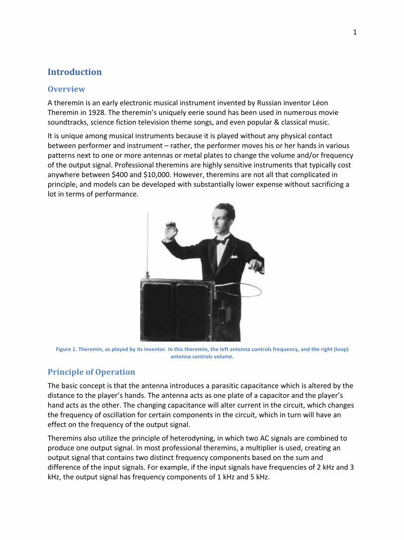
A theremin is an early electronic musical instrument invented by Russian inventor Léon Theremin in 1928. The theremin’s uniquely eerie sound has been used in numerous movie soundtracks, science fiction television theme songs, and even popular & classical music.

It is unique among musical instruments because it is played without any physical contact between performer and instrument – rather, the performer moves his or her hands in various patterns next to one or more antennas or metal plates to change the volume and/or frequency of the output signal. Professional theremins are highly sensitive instruments that typically cost anywhere between $400 and $10,000. However, theremins are not all that complicated in principle, and models can be developed with substantially lower expense without sacrificing a lot in terms of performance.

Figure 1. Theremin, as played by its inventor. In this theremin, the left antenna controls frequency, and the right (loop)

antenna controls volume.

Principle of Operation

The basic concept is that the antenna introduces a parasitic capacitance which is altered by the distance to the player’s hands. The antenna acts as one plate of a capacitor and the player’s hand acts as the other. The changing capacitance will alter current in the circuit, which changes the frequency of oscillation for certain components in the circuit, which in turn will have an effect on the frequency of the output signal.

Theremins also utilize the principle of heterodyning, in which two AC signals are combined to produce one output signal. In most professional theremins, a multiplier is used, creating an output signal that contains two distinct frequency components based on the sum and difference of the input signals. For example, if the input signals have frequencies of 2 kHz and 3 kHz, the output signal has frequency components of 1 kHz and 5 kHz.

2

In many applications, an ideal multiplier is not required and can be replaced with a mixer that uses a small number of components. Simple mixers can be constructed with diodes or transistors. Because heterodyning produces very large sum frequencies, the output of a theremin’s mixer must be passed through a low-pass filter to remove unwanted frequency components.1

Division of Labor

While all group members ended up contributing to all parts of the project, Joe and Matt primarily developed the mixer, and Jason developed the oscillators.

Design Analysis

Top-Level Block Diagram

Figure 2. Top-level block diagram. The pitch null potentiometer is used for calibration of the theremin. More explanation

follows in the oscillator section.

Bench Setup

Figure 3. Bench setup.

3

The system would be powered by a ±15 V supply, the rail voltage of the op-amps. Resistors are used only to reduce the supply voltage to 3 V for the mixer and to reduce the amplitude of the inputs to the mixer.

Wien-Bridge Oscillators

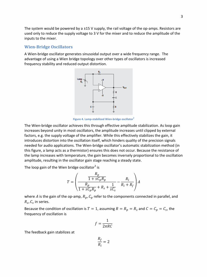
A Wien-bridge oscillator generates sinusoidal output over a wide frequency range. The advantage of using a Wien bridge topology over other types of oscillators is increased frequency stability and reduced output distortion.

Figure 4. Lamp-stabilized Wien-bridge oscillator

2

The Wien-bridge oscillator achieves this through effective amplitude stabilization. As loop gain increases beyond unity in most oscillators, the amplitude increases until clipped by external factors, e.g. the supply voltage of the amplifier. While this effectively stabilizes the gain, it introduces distortion into the oscillation itself, which hinders quality of the precision signals needed for audio applications. The Wien-bridge oscillator’s automatic stabilization method (in this figure, a lamp acts as a thermistor) ensures this does not occur. Because the resistance of the lamp increases with temperature, the gain becomes inversely proportional to the oscillation amplitude, resulting in the oscillator gain stage reaching a steady state.

The loop gain of the Wien bridge oscillator3 is

(

)

where is the gain of the op-amp, refer to the components connected in parallel, and

in series.

Because the condition of oscillation is , assuming and , the

frequency of oscillation is

The feedback gain stabilizes at

4

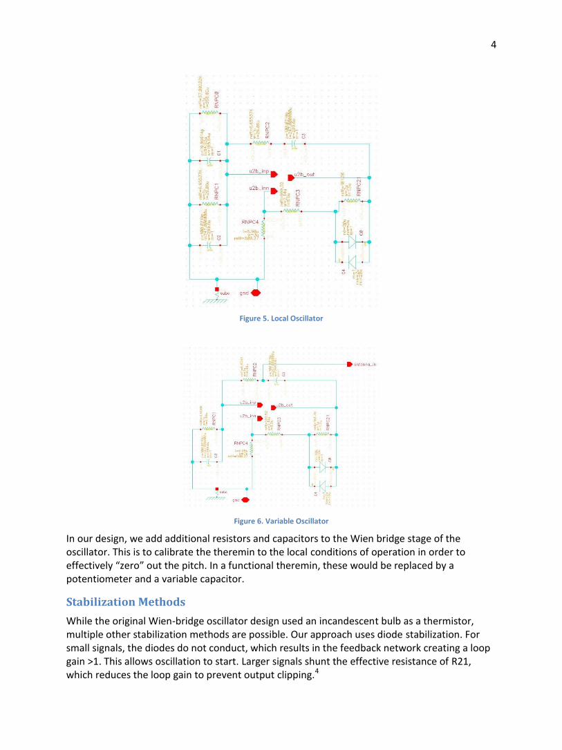
Figure 5. Local Oscillator

Figure 6. Variable Oscillator

In our design, we add additional resistors and capacitors to the Wien bridge stage of the oscillator. This is to calibrate the theremin to the local conditions of operation in order to effectively “zero” out the pitch. In a functional theremin, these would be replaced by a potentiometer and a variable capacitor.

Stabilization Methods

While the original Wien-bridge oscillator design used an incandescent bulb as a thermistor, multiple other stabilization methods are possible. Our approach uses diode stabilization. For small signals, the diodes do not conduct, which results in the feedback network creating a loop gain >1. This allows oscillation to start. Larger signals shunt the effective resistance of R21, which reduces the loop gain to prevent output clipping.4

5

It’s also possible to stabilize using JFETs, for which a higher gate voltage will increase channel resistance, similar to the operation of a thermistor. We were unable to do this because the Cadence packages available to us were not able to fully simulate the operation of JFETs.

Antennae as Variable Capacitors

An antenna acts as a variable capacitor, where the antenna itself acts as one plate and the position of a nearby object (i.e., the player’s hand) can act as the other plate. As one moves one’s hand closer to the antenna, the effective capacitance increases, approximately following an inverse square relationship.

Hand capacitance typically alters this by 1-2 pF, and the antenna will have a fixed capacitance to ground of around 10-15 pF.5

Because these capacitor values are not sufficient to create pleasant output audio frequency levels, two oscillators are necessary such that the difference can create a low enough output frequency.

Heterodyning

Figure 7. Mixer

The mixer takes the two signals from the oscillators and outputs the beat frequency between the two signals, which is the actual signal output of the Theremin. A vital part of how a Theremin functions is based on heterodyning. Heterodyning is a technique developed over a century ago, and remains useful in many electrical engineering applications. This method

6

multiplies two sinusoidal signals and the output is a sum of two other sinusoidal signals, the frequency of one of the output sines is the difference of the two frequencies and the frequency of the other is the sum of the two original frequencies.

( ) ( )

( )

( )

Because the oscillators are running in the realm of 200 kHz, the sum of the two oscillator frequencies is quite high, while the difference is within human hearing range. After the two are combined, the system runs through a low pass filter to remove the high frequency sum. This cleans up the audio output so that it is very nearly just a sine wave at the desired frequency.

The real challenge of this circuit is figuring out a way to multiply the two signals together. In fact, this is impossible to do with only linear components, so we used a BJT and took advantage of the nonlinearity of its operation. The BJT acts as a voltage controlled current source in this configuration, and the output current is proportional to the multiple of the two input sinusoids. Then since the current goes through a resistor in the current emitter-style configuration, the voltage at the collector of the BJT is proportional to the multiple of the oscillator sine waves. After a stage of filtering to clean up the signal, the result is then output.

Op-Amps

The op-amps in our design are vital to the operation of the circuit, but we did not need any specialized parts in order to make it work. Nearly any generic op-amp should be able to be placed instead of our current devices and the system should still work the same. The primary purpose of the op-amps is just for some feedback amplification. Cadence does not have any default op-amps built in, but does have a tool for generating simulated op-amps using Verilog code. It is an automated system that just requests some basic values, like open loop gain, output impedance, and input impedance. We looked up the specs for the NE5532N op-amp, recommended in Harrison’s theremin design, and used these values for our Cadence model.

7

Simulation Results

Figure 8. Oscillator Outputs. Mixer Output is the orange line in the middle. Antenna capacitance is 15pF.

Figure 9. Zoomed in on the Mixer output at antenna capacitance of 15pF. Signal is ~7.5kHz

As seen in Figure 8, the oscillators output very large and similar frequencies. In this case, the local oscillator is outputting around 220 kHz and the variable oscillator is outputting around 212.5 kHz. The mixer is outputting about the difference in frequency of these two inputs at around 7.5 kHz, as seen in Figure 9. The higher frequency can still be seen in the mixer output along the sinusoid, but has been filtered to the point that it has negligible impact on the audio signal.

8

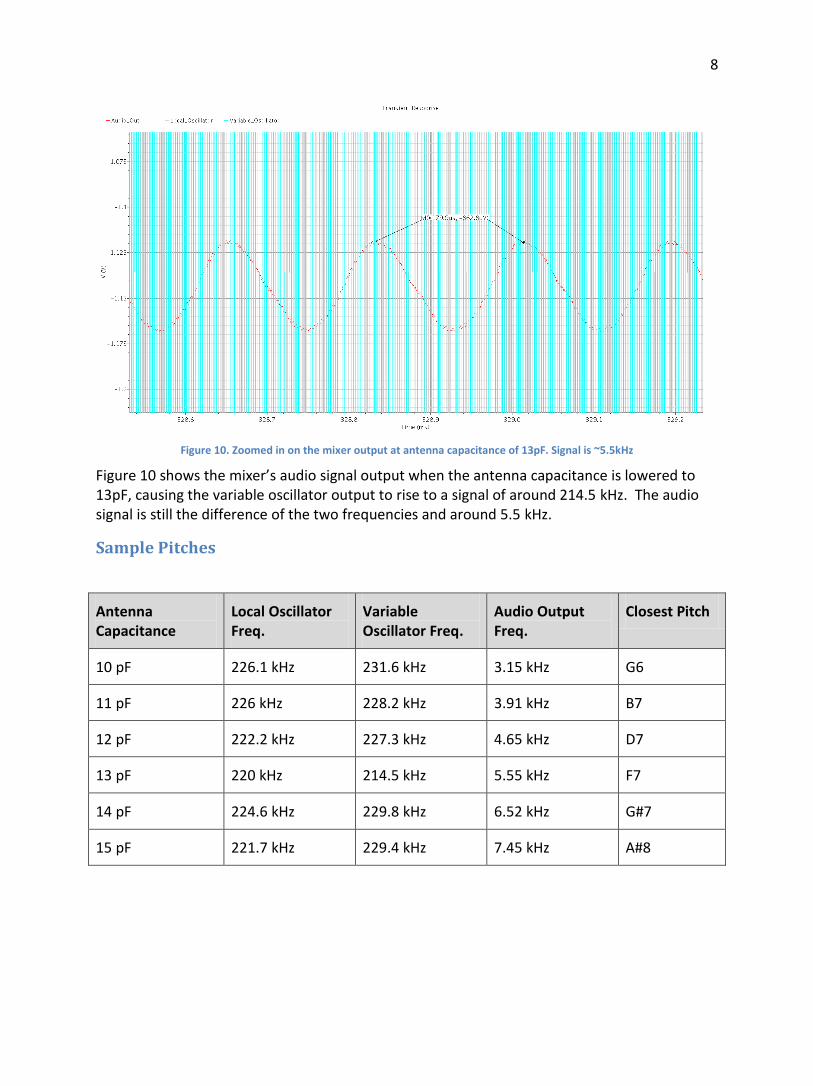
Figure 10. Zoomed in on the mixer output at antenna capacitance of 13pF. Signal is ~5.5kHz

Figure 10 shows the mixer’s audio signal output when the antenna capacitance is lowered to 13pF, causing the variable oscillator output to rise to a signal of around 214.5 kHz. The audio signal is still the difference of the two frequencies and around 5.5 kHz.

Sample Pitches

Antenna Capacitance

Local Oscillator Freq.

Variable Oscillator Freq.

Audio Output Freq.

Closest Pitch

10 pF 226.1 kHz 231.6 kHz 3.15 kHz G6

11 pF 226 kHz 228.2 kHz 3.91 kHz B7

12 pF 222.2 kHz 227.3 kHz 4.65 kHz D7

13 pF 220 kHz 214.5 kHz 5.55 kHz F7

14 pF 224.6 kHz 229.8 kHz 6.52 kHz G#7

15 pF 221.7 kHz 229.4 kHz 7.45 kHz A#8

9

Figure 11. Theremin operation

Discussion

Overall, we felt that our design adequately met specification and had reasonably good performance. The op-amps written in Verilog act as standard commercial op-amps and did not offer design constraints, so we chose to leave them on the bench schematic and lay out the individual circuits as blocks.

We learned that oscillator simulation in Cadence requires introduction of transient noise to start up.

We chose not to optimize for size, in part because it’s irrelevant to the functional application of our circuit. The actual theremin assembly would be far larger than the circuit itself, and the use of an antenna would introduce the necessity of component spacing to prevent interference.

0

1000

2000

3000

4000

5000

6000

7000

8000

10 11 12 13 14 15

Ou

tpu

t Fr

eq

ue

ncy

(H

z)

Capacitance (pF)

Audio_out vs. Antenna Capacitance

10

References

1. Harrison, Arthur. “THE WIEN-BRIDGE THEREMIN.” 16 Jan 2004. <http://theremin.us/200/wien.html>

2. Mancini, Ron. “Design of op amp sine wave oscillators.” Analog Applications Journal, August 2000. <http://www.ti.com/sc/docs/apps/msp/journal/aug2000/aug_07.pdf>

3. Terman, Frederick. Radio Engineers' Handbook, McGraw-Hill Book Company, inc; 1st edition, 1943.

4. Li, Alan. “Programmable Oscillator Uses Digital Potentiometers.” Analog Devices. 2002. <http://www.analog.com/static/imported-files/application_notes/80206653AN580.pdf>

5. American Musical Supply. “Moog Music Etherwave Theremin.” Accessed 25 Nov 2011. <http://www.americanmusical.com/Item--i-MOO-ETHERWAVE-LIST>

11

Appendix

Layout

Figure 12. Local Oscillator layout.

Figure 13. Variable Oscillator layout.

12

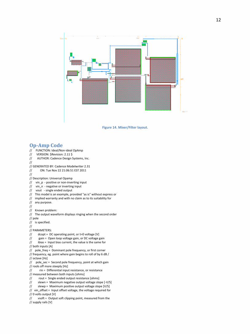
Figure 14. Mixer/Filter layout.

Op-Amp Code // FUNCTION: Ideal/Non-ideal OpAmp // VERSION: $Revision: 2.11 $ // AUTHOR: Cadence Design Systems, Inc. // // GENERATED BY: Cadence Modelwriter 2.31 // ON: Tue Nov 22 21:06:51 EST 2011 // // Description: Universal Opamp // vin_p - positive or non-inverting input // vin_n - negative or inverting input // vout - single ended output // This model is an example, provided "as is" without express or // implied warranty and with no claim as to its suitability for // any purpose. // // Known problem: // The output waveform displays ringing when the second order // pole // is specified. // // PARAMETERS: // dcopt = DC operating point, or t=0 voltage [V] // gain = Open loop voltage gain, or DC voltage gain // ibias = Input bias current, the value is the same for // both inputs [A] // pole_freq = Dominant pole frequency, or first corner // frequency, eg. point where gain begins to roll of by 6 dB / // octave [Hz] // pole_sec = Second pole frequency, point at which gain // rools off more steeply [Hz] // rin = Differential input resistance, or resistance // measured between both inputs [ohms] // rout = Single ended output resistance [ohms] // slewn = Maximum negative output voltage slope [-V/S] // slewp = Maximum positive output voltage slope [V/S] // vin_offset = Input offset voltage, the voltage required for // 0 volts output [V] // vsoft = Output soft clipping point, measured from the // supply rails [V]

13

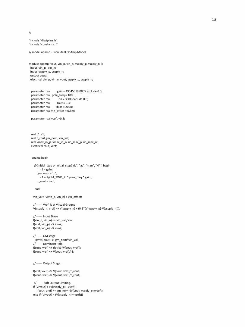
// `include "discipline.h" `include "constants.h" // model opamp - Non Ideal OpAmp Model module opamp (vout, vin_p, vin_n, vspply_p, vspply_n ); inout vin_p , vin_n; inout vspply_p, vspply_n; output vout; electrical vin_p, vin_n, vout, vspply_p, vspply_n; parameter real gain = 49545019.0805 exclude 0.0; parameter real pole_freq = 100; parameter real rin = 300K exclude 0.0; parameter real rout = 0.3; parameter real ibias = 200n; parameter real vin_offset = 0.5m; parameter real vsoft =0.5; real c1, r1; real r_rout,gm_nom, vin_val; real vmax_in_p, vmax_in_n, iin_max_p, iin_max_n; electrical cout, vref; analog begin @(initial_step or initial_step("dc", "ac", "tran", "xf")) begin r1 = gain; gm_nom = 1.0; c1 = 1/(`M_TWO_PI * pole_freq * gain); r_rout = rout; end vin_val= V(vin_p, vin_n) + vin_offset; // ------ Vref is at Virtual Ground V(vspply_n, vref) <+ V(vspply_n) + (0.5*(V(vspply_p)-V(vspply_n))); // ------ Input Stage I(vin_p, vin_n) <+ vin_val / rin; I(vref, vin_p) <+ ibias; I(vref, vin_n) <+ ibias; // ------ GM stage I(vref, cout) <+ gm_nom*vin_val ; // ------ Dominant Pole. I(cout, vref) <+ ddt(c1*V(cout, vref)); I(cout, vref) <+ V(cout, vref)/r1; // ------ Output Stage. I(vref, vout) <+ V(cout, vref)/r_rout; I(vout, vref) <+ V(vout, vref)/r_rout; // ------ Soft Output Limiting. if (V(vout) > (V(vspply_p) - vsoft)) I(cout, vref) <+ gm_nom*(V(vout, vspply_p)+vsoft); else if (V(vout) < (V(vspply_n) + vsoft))

14

I(cout, vref) <+ gm_nom*(V(vout, vspply_n)-vsoft); end endmodule