World Institute for Development Economics Research wider.unu.edu

WIDER Working Paper 2014/135

An integrated approach to modelling energy policy in South Africa

Evaluating carbon taxes and electricity import restrictions

Channing Arndt,1 Rob Davies,2 Sherwin Gabriel,2 Konstantin Makrelov,2 Bruno Merven,3 Faaiqa Salie,2 and James Thurlow4

October 2014

1UNU-WIDER; 2Economic Policy, National Treasury of South Africa; 3Energy Research Centre, University of Cape Town; 4International Food Policy Research Institute; corresponding author: Channing@wider.unu.edu

This study has been prepared within the UNU-WIDER project ‘Regional Growth and Development in Southern Africa’, directed by Channing Arndt

Copyright © UNU-WIDER 2014

ISSN 1798-7237 ISBN 978-92-9230-856-8

Typescript prepared by Ayesha Achari for UNU-WIDER.

UNU-WIDER gratefully acknowledges the financial contributions to the research programme from the governments of Denmark, Finland, Sweden, and the United Kingdom.

The World Institute for Development Economics Research (WIDER) was established by the United Nations University (UNU) as its first research and training centre and started work in Helsinki, Finland in 1985. The Institute undertakes applied research and policy analysis on structural changes affecting the developing and transitional economies, provides a forum for the advocacy of policies leading to robust, equitable and environmentally sustainable growth, and promotes capacity strengthening and training in the field of economic and social policy-making. Work is carried out by staff researchers and visiting scholars in Helsinki and through networks of collaborating scholars and institutions around the world.

UNU-WIDER, Katajanokanlaituri 6 B, 00160 Helsinki, Finland, wider.unu.edu

The views expressed in this publication are those of the author(s). Publication does not imply endorsement by the Institute or the United Nations University, nor by the programme/project sponsors, of any of the views expressed.

Abstract: We link a bottom-up energy sector model to a recursive dynamic computable general equilibrium model of South Africa in order to examine two of the country’s main energy policy considerations: (i) the introduction of a carbon tax and (ii) liberalization of import supply restrictions in order to exploit regional hydropower potential. Our results suggest substantial reductions in the country’s greenhouse gas emissions when these two policy changes are jointly implemented (relative to business-as-usual baseline scenario). Moreover, the two policies impose essentially no cost to economic growth, although there is a 1 per cent reduction in employment. From our analysis we conclude that a regional energy strategy, anchored in hydropower, represents a potentially inexpensive approach to reducing emissions in South Africa. Moreover, combining carbon taxes with a removal of import restrictions lessens the burden of adjustment on politically sensitive and economically important sectors.

Keywords: integrated bottom-up model, the integrated MARKAL-EFOM system, computable general equilibrium, carbon tax, South Africa JEL classification: O55, Q43, Q47, Q49

1

1 Introduction

Energy is vital for economic development. This was recently illustrated in South Africa, where recent and widespread electricity shortages constrained economic activity (Inglesi 2010). This prompted the government to propose a new long-term energy investment plan (DOE 2011). At the same time, the country committed itself to reducing its greenhouse gas (GHG) emissions, half of which are from electricity generation (Arndt et al. 2013). However, investing in new and cleaner energy can incur significant tradeoffs, most obviously in the form of higher energy prices. This may lead to slower economic growth, job losses, and a higher cost of living for low-income households—each of which is a major policy concern for South Africa (Resnick et al. 2012). As such, long-term energy investment plans, particularly in developing countries, need to not only meet future energy needs (and environmental commitments) but also limit any potential socioeconomic tradeoffs.

It is standard practice in energy planning to use detailed bottom-up energy sector models. However, a shortcoming of this approach is that it fails to take into account the demand response of proposed energy paths and, therefore, only provides a rough estimate of the optimal build-plan. Another approach is to combine an energy sector model with a computable general equilibrium model that can measure demand responses. However, full inter-temporal integration usually constrains the level of detail in general equilibrium models (GEMs), thus limiting their usefulness for policy analysis, including measuring how energy prices affect socioeconomic outcomes, such as employment and incomes.

In this paper, we present an iterative approach to energy planning that addresses some of the shortcomings already mentioned while maintaining the attractive features of detailed energy sector and GEMs. The paper focuses on electricity planning in South Africa. Section 2 presents a recursive dynamic approach to model integration which extends existing studies that typically opt for full optimization at the cost of using lower-resolution economic models. In Section 3, we examine two of South Africa’s major energy policies currently under consideration: (i) the introduction of a carbon tax and (ii) the removal of electricity import restrictions. In the final section, we conclude by drawing lessons for South Africa.

2 Integrated Modelling Framework

We adopt the approach advocated by Lanz and Rausch (2011), that is, an integrated bottom-up energy sector and general equilibrium model. The authors show that this approach allows for the combination of model strengths that enable the assessment of policy changes on energy prices, demand, and welfare as well as the identification of possible abatement opportunities. They find that this methodology is superior to independent partial equilibrium models, which fail to account for the secondary impacts of shocks. It is also an improvement on independent GEMs, which do not accurately capture changes in fuel substitution because of their lack of detailed energy technology information. Various studies adopt the integrated bottom-up approach (see e.g. Böhringer and Rutherford 2009; Tuladhar et al. 2009).

Our approach differs from those of existing studies in that we link the energy sector and GEMs via a recursive dynamic process. By avoiding using forward-looking inter-temporal dynamics in the general

2

equilibrium model, it is possible to retain a higher resolution depiction of the economy that is more useful for simulating policies and measuring socioeconomic outcomes. Since both models appear in the literature, we briefly describe their main characteristics before discussing model integration and convergence.

2.1 Energy sector model

We use a version of The Integrated MARKAL-EFOM System (TIMES), known as the South African TIMES Model (SATIM). SATIM is an inter-temporal bottom-up partial equilibrium optimization model of the energy sector (see Energy Research Centre System Analysis and Planning Group 2013). In the full version of SATIM, demand is for ‘useful energy’, for example, demand for energy services such as cooking, lighting, and heating. Final energy demand is determined endogenously on the basis of the optimal mix of technologies. This allows for tradeoffs between demand and supply sectors, and explicitly captures process changes, fuel and mode switching, and technical or efficiency improvements.

We use a version of SATIM that only includes the power sector module. It computes the least-cost mix of power plants, in terms of capacity and production, over a defined planning horizon. This is derived from an optimization problem, where the objective function is to minimize the discounted future capital and operating costs of power plants. SATIM uses linear or mixed integer programming to solve the least-cost planning problem subject to a series of constraints and system parameters. Constraints include future electricity demand, required reserve margins, and resource limits (e.g. fossil fuel reserves and renewable energy potential). System parameters include load curves, fuel prices and availability, the existing stock of power plants (i.e. efficiencies, running costs, and retirement profiles), and new power plant options (i.e. investment costs, capacity factors, and construction times).

SATIM enables us to simulate two of South Africa’s main energy policy considerations. First, SATIM allows us to impose the current restrictions on imported electricity. These restrictions may become a binding constraint on the choice of power plant mix given the considerable potential for neighbouring countries to supply hydropower and coal-fired electricity to the South African market via the Southern African Power Pool (i.e. an integrated regional network of transmission infrastructure). Second, SATIM can incorporate carbon taxes on GHG emissions through changes in fossil fuel prices.

Limitations of SATIM

Econometric methods that rely on time-series data are often inadequate for long-term demand projections, and thus scenario-based approaches have to be used. This approach, unlike forecasts, does not presuppose knowledge of the main drivers of demand (e.g. economic growth, technological improvements and choices, and energy prices). Instead, a scenario consists of a set of coherent assumptions about the future trajectories of the drivers leading to a coherent system, which can form the basis for a credible storyline for each scenario. This can be very difficult to achieve without using some form of economic model.

SATIM can be used to analyse energy policies, such as renewable energy targets or a nuclear programme. However, while the impact of these policies on electricity prices and GHG emissions can be estimated, it is not possible to quantify economywide implications, including backward and forward linkages, without the help of some form of an economic model. For example, switching to more

3

expensive renewable energy in SATIM may cause electricity prices to increase. However, the extent to which higher prices lowers electricity demand is not captured in SATIM.

Input assumptions for SATIM

The version of SATIM used here has been aligned with the South African Integrated Resource Plan (IRP) (DOE 2011), with some adjustments detailed in Appendix A. Where it differs is with regard to how much electricity may be imported. The IRP has around 4.5 GW of additional hydropower import options, which does not include Inga. We consider the more extreme hypothetical case of almost 40 GW being available in the region for South Africa to import. The cost assumptions for the additional hydropower option are also detailed in Appendix A.

2.2 Economic model

We use the South African General Equilibrium (SAGE) model, which is a recursive dynamic country level, economywide model. This is a dynamic variant of the generic static model described by Lofgren et al. (2002) and is a descendant of the class of computable general equilibrium model introduced by Dervis et al. (1982). The core structure and dynamics of the SAGE model have been described by Diao and Thurlow (2012).

Figure 1 provides a representation of SAGE’S economywide structure that links sectoral patterns of economic growth to changes in the incomes of different household groups. SAGE simulates the functioning of the South African economy and provides useful insights on the direct and indirect linkages that connect different groups of profit-maximizing producers and utility-maximizing households, as well as the government and the rest of the world. SAGE provides a detailed and comprehensive representation of the economy, including 62 industries, 49 products, 9 factors of production, and 14 representative household groups. This information is drawn from a 2007 version of the Social Accounting Matrix described by Davies and Thurlow (2013) and was reconciled with the 2007 Energy Balance (DOE 2012). As seen in Figure 2, SAGE’s energy sector comprises nine electricity and four fuel production technologies.

4

Figure 1: Economy-wide structure and linkages in the SAGE model

Source: Authors’ representation of the SAGE model.

Figure 2: Structure of the energy sector in the SAGE model

Source: Authors’ representation of the SAGE model.

Public investment

Production

Economic growth

Agriculture

Industry

Services

Factor markets

Product

Household welfare

Agriculture

Industry

Services

Payments Incomes

Consumptio

Government

Rest of the world Taxes

Recurrent spending

Taxes Trade

Borrowing

Taxes, grants

Productivity

Capital supply

Foreign investment

Savings, private

Coal-fired

Nuclear

Hydropower

Solar (photovoltaic)

Solar (thermal)

Wind

Gas-fired

Diesel

Imports

Coal-to-liquid

Gas-to-liquid

Refined oil

Natural gas

Coal

Crude oil

Electricity

Petroleum

5

SAGE’s recursive dynamic structure consists of within- and between-period components. Within each time period, SAGE is solved subject to given levels of population, productivity, and capital supply. One important feature of SAGE is that non-energy industries can respond to rising energy prices by investing in less energy-intensive technologies, subject to investment financing constraints (see Alton et al. 2014). Between periods, SAGE is updated to reflect population growth, technical change, and capital accumulation. The accumulation of capital is determined endogenously on the basis of previous period investment levels. New capital is allocated to sectors on the basis of their relative profit rates. Once invested, capital becomes sector-specific. This specification partly captures the adjustment costs from reorienting production across industries of different energy and carbon intensities. All new power plant investments are financed through a regulated electricity tariff that amortizes the debt and covers the operating and maintenance costs incurred by South Africa’s primary electricity provider, Eskom, which is an independently managed state enterprise. Finally, at the macroeconomic level, we assume that nominal private and public consumption and investment spending are fixed proportions of total absorption, and that the real exchange rate adjusts to maintain an exogenously determined current account balance.

Trade, production, and household income elasticities used in SAGE are consistent with those used by Alton et al. (2014).

Limitations of SAGE

The allocation of productive resources in a CGE model is based on changes in relative prices. This means that the model is not ideally suited to analysing investments in different electricity-generating technologies, since the rationale for these allocation decisions often requires some technical considerations, such as the demand and renewable energy resource profiles. As these factors are not incorporated in SAGE, it is preferable to use a model like SATIM that has a more detailed representation of energy technologies and demand profiles.

2.3 Model integration

We formally link SATIM and the SAGE model in a way that retains the best features of both (i.e. one that captures detailed energy investment options), as well as detailed information on economic structure and behaviour. Within our linked framework, SATIM computes an optimal power plant investment plan based on forecasted electricity demand and fossil fuel prices from SAGE. SAGE replicates the power plant mix and associated electricity price from SATIM, and then revises its electricity demand and fuel price forecasts.

Our model integration differs from existing approaches in two respects. First, most studies that iterate between models do so at a given point in time until a consistent solution is reached. In contrast, we treat this as a rolling procedure in which each iteration reflects a gradual movement over time towards consistency. Our specification only produces significantly different results if there are long time intervals between iterations; that is, if there is insufficient opportunity for adjustments to avoid an undersupply or oversupply of electricity before the build plan is revised. This is a possibility in South Africa, where investment plans are typically revised once every decade, and where proposed changes to energy policies introduce uncertainty into the planning process.

6

Second, when solving the economic model, we aggregate the individual electricity technologies shown in Figure 2 into a single composite sector consisting of a weighted combination of the planned plant mix from SATIM. This allows the general equilibrium model to endogenously determine future levels of electricity demand and supply, such as in response to changing policies and electricity prices, while also retaining the projected power plant mix from SATIM. The assumption is that any under-utilization of capacity that may occur within SAGE is uniformly distributed across power plants. The convergence procedure leads to a minimum cost power plant mix that meets current and future demand levels that are consistent with a regulated electricity price projection. This price projection is itself sufficient to finance the build and operation costs of the system.

Figure 3 illustrates the solution process. The simulation period (shown on the horizontal axis) consists of three sub-periods: committed, forecast, and extended. During the committed period (solid black line), no changes to the power plant mix and electricity supply levels are permitted. This period consists of historical years, whose investments cannot be undone. The forecast period (dashed black line) includes years that are of economic interest (shown as 2010–30 in the figure), whereas the extended period (dashed grey line) covers the longer planning horizon of the energy sector (shown as 2030–40 in the figure).1 The latter is necessary because investments in power plants have long lead times, such that a new plant only starting to produce electricity during the extended period may still impose investment costs that affect economic outcomes during the forecast period.

The SAGE model is initially run with expected policies (e.g. with or without a carbon tax) and with expected values for exogenous parameters (e.g. world fossil fuel prices). During the first iteration, we impose the existing electricity build plan from the Department of Energy (DOE 2011) for the period 2007–10. Results from SAGE provide a consistent set of inputs to SATIM, including electricity demand targets, fuel prices, and investment costs. SATIM uses these inputs to revise the build plan, which may differ from the current plan if technologies, expected policies, demand forecasts, and input cost expectations change. The revised build plan, including investment costs and electricity prices, is then imposed on SAGE and the process is repeated. Note that the ‘current’ time period moves forward after each coupled run (down the vertical axis), such that the committed period becomes longer with each iteration. This process continues until a committed build plan is obtained for the entire forecast period. The final solution from SAGE reflects the economic implications of the final power plant build plan.

1 The modelling framework permits one to choose the period of economic interest and the additional forecast period. The actual period choices are discussed later.

7

Figure 3: Illustrative representation of model integration

Source: Authors’ representation of the SATIM–SAGE model.

2.4 Model convergence

The speed at which SATIM and SAGE converge on a build plan that is consistent with long-run electricity demand and prices depends on the time interval between iterations. Figure 4 shows the level of electricity demand in 2030 after each iterative coupled run. This is done for a baseline scenario and a scenario that includes a carbon tax (see Section 3). Note that a movement along the horizontal axis in Figure 4 corresponds to a movement down the vertical axis in Figure 3.

There is strong model convergence after two iterations. For example, starting from a 2006 base year for SATIM, the projected electricity demand for 2030 in the baseline scenario stabilizes at around 550 GWh by 2008 when the coupled run interval is one year. It converges to this value by 2010 when the interval is two years, and by 2014 when the interval is four years. Therefore, to ensure convergence between SATIM and SAGE for our period of interest (i.e. 2010–35), we assign two-year intervals between coupled runs during the four years when we have historical data on the electricity supply mix (i.e. 2006–10) and five-year intervals during the forecast period (i.e. 2010–40). The latter is motivated by South Africa’s goal of revising its future energy investment plans more frequently than it has done in the past. Finally, SATIM’s extended optimization period runs until 2070 on the basis of a long-run demand forecast from SAGE, which, after 2040, is only solved every five years rather than annually.

SAGE

SAGE

SATIM

SAGE

SATIM

2010 2020 2030 2040 2007

2010

2020

2030

Forecast period in annual time steps

Iter

ativ

e co

uple

d

Committed Forecast Extended

SAGE

SATIM

Electricity production mix

Final electricity price

Plant construction investment costs

Electricity demand

Fossil fuel prices

8

Figure 4: Model convergence under different coupled run intervals

Source: Results from the SATIM–SAGE model.

3 Evaluating energy policies

In this section, we use the integrated models to examine two major energy policies that South Africa is currently considering. The first is a carbon tax. In 2012, the South African government announced its intention to implement a carbon tax in order to reduce national GHG emissions by two-thirds, relative to a ‘business-as-usual’ baseline. This is ambitious, given that 92.7 per cent of South Africa’s electricity supply in 2007 was from coal-fired plants fed from cheap and plentiful domestic coal reserves (DOE 2012). Using the SAGE model, Alton et al. (2014) estimated that a carbon tax of US$30 per ton of carbon dioxide (CO2)-equivalent emissions would be needed to meet the emissions target, and that this tax will lower gross domestic product (GDP) and employment by 1.2 and 0.6 per cent, respectively, relative to a untaxed baseline. However, the authors did not consider how the carbon tax might change the current electricity sector investment plan. Moreover, by treating the build plan as independent of the carbon tax, they also did not consider the investment cost of the current plan’s modest reduction in electricity emissions. In this paper, we simulate a similar carbon tax, but allow for revisions to the build plan in response to the carbon tax and fully internalize investment costs via a regulated electricity price.

The second policy is the lifting of restrictions on imported electricity. There is substantial hydropower potential within southern Africa, particularly along the Congo and Zambezi Rivers. For example, the Grand Inga dam’s potential capacity is almost equal to South Africa’s total generation capacity in 2005. In contrast, South Africa’s ability to expand domestic hydropower is limited. Moreover, while the current investment plan includes nuclear, solar, and wind options, expanding their use will substantially increase investment costs and electricity prices (DOE 2011).2 One major constraint to exploiting the

2 This is, of course, based on the technology assumptions prevailing at the time.

480

490

500

510

520

530

540

550

560

2006 2010 2014 2018 2022 2026

Ele

ctri

city

dem

and

in 2

030

(GW

h)

Year of coupled run

Coupled runs every year

Coupled runs every two years

Coupled runs every four years

Baseline

Carbon Tax

9

renewable energy potential in neighbouring countries is the current restriction on how much electricity can be imported into South Africa, ostensibly to ensure the security of energy supply. We simulate the effect of removing this restriction, both with and without a carbon tax.

3.1 Baseline scenario

We first establish a baseline in which there are no carbon taxes or changes to import policy. Following Alton et al. (2014), we assume that the supply of secondary and tertiary-educated labour expands exogenously at 1.5 and 1.0 per cent per year, respectively, while the supply of primary-educated labour is determined endogenously by an upward sloping supply curve.3 Capital stocks grow at 4 per cent per year on the basis of accumulated savings and investment. The rate of technical change is initially a uniform 1 per cent per year in all sectors, with a gradual deceleration over time in order to stabilize long-run economic growth rates. Changes in global agricultural and fossil fuel prices are based on the reference scenario in the study by Sokolov et al. (2009), which excludes any global policy to reduce GHG emissions. These projections imply that South Africa’s terms-of-trade will deteriorate by one-fifth over the next three decades.4

In addition, real government consumption grows by 3.0 per cent per year over the simulation period, while sales taxes adjust to maintain a fixed budget balance. Foreign savings are assumed to expand by 2.0 per cent annually. Land may be repurposed for different activities, and its availability expands initially by 1.0 per cent, slowing over time.

These assumptions produce an average total GDP growth rate of 3.5 per cent per year over the simulation period (i.e. 2010–35). This is faster than the growth in electricity supply, causing real electricity prices to increase, particularly over the short-run when supply responses are constrained by rising coal prices, inadequate past investment in power plants, and long construction lead times. Rising incomes and energy demand causes per capita CO2 emissions to rise from 9.3 tons per person in 2010 to 13.3 tons in 2035. Almost half of all emissions in 2035 are from electricity generation. This is in spite of rising electricity prices and improvements in the energy efficiency of industrial users. There is little change in the power plant mix, with coal-fired plants still accounting for 86.3 per cent of electricity supply in 2035. This baseline scenario is quite consistent with the ‘base case’ projection in the current investment plan (see DOE 2011).

3.2 Policy scenarios

We consider three policy scenarios. In the first simulation, called Carbon Tax, we gradually introduce a carbon tax starting at US$3 (or 21 ZAR at 2007 prices and exchange rates) per ton of CO2 equivalent in 2015, rising to US$30 by 2024, and remaining constant thereafter. We impose the tax on fossil fuels on the basis of standard emission factors. The tax is applied to domestically combusted primary fuels and the estimated CO2 content of imports. Tax rebates are provided to exports on the basis of their estimated CO2 content (see Alton et al. 2014). Carbon tax revenues are principally recycled through a

3 The elasticity of supply with respect to real wages is 0.1, which produces an overall employment growth elasticity of approximately 0.67, which is consistent with recent observations for South Africa. 4 Coal, crude oil, and natural gas prices increase by 20, 122, and 103 per cent, respectively, over the period 2010–2040. Similarly, agricultural and food prices rise by 17 per cent.

10

uniform reduction in indirect tax rates, which is a relatively ‘distribution neutral’ recycling option since all industries and households benefit from lower producer and product taxes. In the second simulation, called Import Policy, we relax the restriction on imported hydropower without introducing the carbon tax. We assume that the region has a total hydropower capacity equivalent to that of the Grand Inga dam, although this is not a binding constraint in our analysis. Finally, in the third simulation, called ‘Tax with Imports’, we simulate both the carbon tax and the lifting of import restrictions at the same time.

Other assumptions and model closures applied in the baseline scenario are also applied in the three policy scenarios.

Figure 5a–c shows deviations from the baseline for total electricity demand, the regulated (average) electricity price, and total GHG emissions, respectively. Figure 6 shows the corresponding electricity supply mixes in 2025 and 2035. Key energy and socioeconomic outcomes are presented in Tables 1 and 2, respectively.

Figure 5: Deviation in (a) total electricity demand, (b) regulated (average) electricity prices, and total GHG emissions from baseline, 2010–35

(a)

(b)

-9-8-7-6-5-4-3-2-1012

2010 2015 2020 2025 2030 2035

Cha

nge

from

bas

elin

e (%

)

-10

0

10

20

30

40

50

2010 2015 2020 2025 2030 2035

Cha

nge

from

bas

elin

e (%

)

11

(c)

Source: Results from the SATIM–SAGE model.

Figure 6: Electricity supply mix in 2010, 2025, and 2035

Source: Results from the SATIM–SAGE model.

-25

-20

-15

-10

-5

0

5

2010 2015 2020 2025 2030 2035

Cha

nge

from

bas

elin

e (%

)

Carbon Tax Import policy Tax with imports

0

100

200

300

400

500

600

Baseline Baseline Carbon tax Importpolicy

Tax withimports

Baseline Carbon tax Importpolicy

Tax withimports

2010 2025 2035

Ele

ctri

city

sup

ply

(GW

h)

Coal Nuclear Renewables Imported Diesal, gas and waste

12

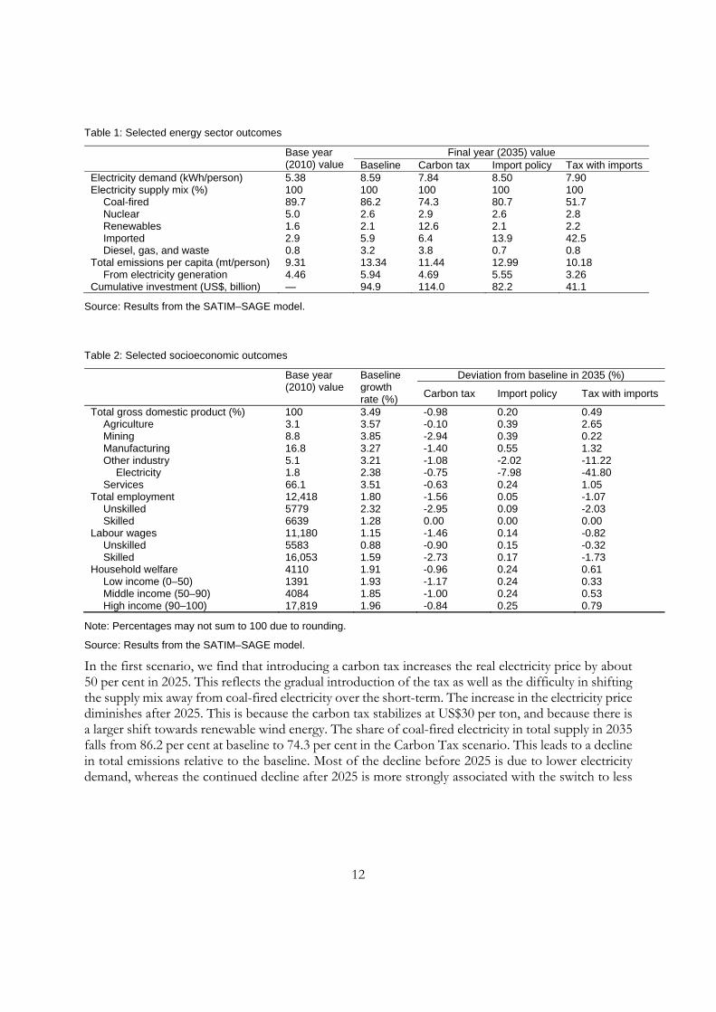
Table 1: Selected energy sector outcomes

Base year (2010) value

Final year (2035) value Baseline Carbon tax Import policy Tax with imports Electricity demand (kWh/person) 5.38 8.59 7.84 8.50 7.90 Electricity supply mix (%) 100 100 100 100 100

Coal-fired 89.7 86.2 74.3 80.7 51.7 Nuclear 5.0 2.6 2.9 2.6 2.8 Renewables 1.6 2.1 12.6 2.1 2.2 Imported 2.9 5.9 6.4 13.9 42.5 Diesel, gas, and waste 0.8 3.2 3.8 0.7 0.8

Total emissions per capita (mt/person) 9.31 13.34 11.44 12.99 10.18 From electricity generation 4.46 5.94 4.69 5.55 3.26

Cumulative investment (US$, billion) — 94.9 114.0 82.2 41.1

Source: Results from the SATIM–SAGE model.

Table 2: Selected socioeconomic outcomes

Base year (2010) value

Baseline growth rate (%)

Deviation from baseline in 2035 (%)

Carbon tax Import policy Tax with imports

Total gross domestic product (%) 100 3.49 -0.98 0.20 0.49 Agriculture 3.1 3.57 -0.10 0.39 2.65 Mining 8.8 3.85 -2.94 0.39 0.22 Manufacturing 16.8 3.27 -1.40 0.55 1.32 Other industry 5.1 3.21 -1.08 -2.02 -11.22

Electricity 1.8 2.38 -0.75 -7.98 -41.80 Services 66.1 3.51 -0.63 0.24 1.05

Total employment 12,418 1.80 -1.56 0.05 -1.07 Unskilled 5779 2.32 -2.95 0.09 -2.03 Skilled 6639 1.28 0.00 0.00 0.00

Labour wages 11,180 1.15 -1.46 0.14 -0.82 Unskilled 5583 0.88 -0.90 0.15 -0.32 Skilled 16,053 1.59 -2.73 0.17 -1.73

Household welfare 4110 1.91 -0.96 0.24 0.61 Low income (0–50) 1391 1.93 -1.17 0.24 0.33 Middle income (50–90) 4084 1.85 -1.00 0.24 0.53 High income (90–100) 17,819 1.96 -0.84 0.25 0.79

Note: Percentages may not sum to 100 due to rounding.

Source: Results from the SATIM–SAGE model.

In the first scenario, we find that introducing a carbon tax increases the real electricity price by about 50 per cent in 2025. This reflects the gradual introduction of the tax as well as the difficulty in shifting the supply mix away from coal-fired electricity over the short-term. The increase in the electricity price diminishes after 2025. This is because the carbon tax stabilizes at US$30 per ton, and because there is a larger shift towards renewable wind energy. The share of coal-fired electricity in total supply in 2035 falls from 86.2 per cent at baseline to 74.3 per cent in the Carbon Tax scenario. This leads to a decline in total emissions relative to the baseline. Most of the decline before 2025 is due to lower electricity demand, whereas the continued decline after 2025 is more strongly associated with the switch to less

13

carbon-intensive energy. Renewables, which exhibit little change at baseline, are made more cost-competitive by the carbon tax.5

Total GDP and employment are 1.0 and 1.6 per cent lower in 2035, respectively, than they would have been without the carbon tax. The cumulative investment cost over 2010–35 at baseline is US$95 billion (in 2007 prices). This increases to US$114 billion—equivalent to 40 per cent of the total GDP in 2010—in the Carbon Tax scenario.6 This higher investment cost is due to renewables being more expensive than coal-fired electricity. A higher electricity price is therefore needed to cover the higher operating and capital costs of total installed system capacity, causing production costs to rise in all sectors. The carbon tax, therefore, lowers GDP both by reducing the returns to installed capital and by substantially raising electricity prices. The negative effects of the carbon tax are larger on more energy-intensive industrial sectors, such as metals and chemicals (see Appendix Table A1).

In the second scenario, we relax the restriction on imported hydropower without introducing a carbon tax. This increases the share of imported electricity in total supply from 5.9 per cent at baseline in 2035 to 13.9 per cent in the Import Policy scenario. This suggests that imported hydropower is cost-competitive against domestic coal-fired electricity. However, the effect on the long-run supply mix is fairly modest. Even though the cumulative investment costs are 13.4 per cent lower than at baseline, there is still only a small decline in the electricity price and, hence, only a small increase in long-run electricity demand. This is reflected in the slight increase in total GDP and negligible change in total employment. Gains in the non-energy sectors are offset by a contraction of the electricity sector, because of less investment in domestic coal- and gas-fired power plants relative to the baseline. This explains the (modest) reduction in total emissions by 2035. Our results suggest that simply removing the restrictions on imported hydropower will not substantially reduce GHG emissions. Thus, while removing import restrictions is beneficial for most sectors, it is not a substitute for a carbon tax.

In the final scenario, we combine the lifting of import restrictions with a carbon tax. Results suggest that the combination of a carbon tax and a policy to pursue regional energy options provides a small GDP growth benefit compared with the Import Policy scenario discussed earlier. This GDP benefit appears even though employment levels are about 1 per cent lower. The result suggests, once again, that imported hydropower from Grand Inga competes broadly on a par with domestic coal-fired power generation. The combination of lifting import restrictions and applying a carbon tax allows for a substantial shift towards imported hydropower, which represents 42.5 per cent of the supply mix by 2035.

It is reasonable to ask why a higher level of imported hydropower was not chosen in the Import Policy scenario given that the resource allocations in the Tax with Imports scenario provide a small growth benefit and were available to the Import Policy scenario. This small growth benefit, of about 0.3 per cent of baseline GDP in 2035, arises from two principal sources. First, the price shifts induced by the carbon tax reduce the relative prices of investment goods. For the same nominal investment (recall that the closure rule implies nominal investment is a fixed share of total nominal absorption), more

5 At higher carbon tax rates, nuclear power substantially substitutes for coal. 6 South Africa’s Department of Energy (DOE 2011) estimates a cumulative investment cost of US$108 billion in their ‘base case’ scenario. This is higher than our estimate, mainly because we include a decline in electricity demand in response to rising electricity prices.

14

real investment can be obtained. Because import liberalization greatly reduces the level of investment in new domestic power plants (cumulative investment costs in the Tax with Imports scenario is US$41.1 billion, which is 57 per cent lower than at baseline and 64 per cent lower than in the Carbon Tax scenario), the resources that would have been invested in more expensive renewables can now be invested in other sectors of the economy. The reduction in the investment price index induced by the carbon tax provides an incremental bonus. Second, the choice of 2035 as our final year of analysis captures the Import Policy scenario in the midst of building a number of new power plants. Some investment has been sunk into plant construction; however, the plants are not all complete and, hence, do not add to GDP in 2035. In the Imports with Tax scenario, there is essentially zero power plant construction in process in 2035; hence, by assumption, all investment has been converted to productive capital.

In sum, although our results should not be interpreted as pointing to a robust interaction between carbon tax and imported power that actually spurs growth beyond what would be obtained from imports alone, they do strongly suggest the possibility of extraordinarily inexpensive emissions reductions, at least in terms of foregone GDP growth. If we value the total emissions avoided in the Import with Tax scenario (Import with Tax minus Baseline) at the value of the carbon tax imposed, the net present value of the pollution costs avoided, discounted to the end of 2014, amount to more than US$20.8 billion (at actual 2007 prices). In the modelling conducted here, these (globally distributed) gains come at no GDP cost to the South African economy, though they do impose a 1ºper cent reduction in the level of employment.

Of course, numerous potential costs to imported power are not included in the model employed here. Not least among these is the cost of system failure due to violence or terrorism in the region. In the absence of environmental externalities from mining and burning fossil fuels, particularly coal, South Africa would be well advised to continue to exploit its coal reserves for power generation. However, consideration of environmental externalities may shift the calculus completely. Viewed globally, the gains from imported hydropower are potentially very large and certainly merit due consideration.7

Finally, it is worthwhile mentioning that the major beneficiaries of the combined import liberalization and carbon tax policy are sectors such as metals and chemicals, which are also the worst affected when only a carbon tax is implemented (see Appendix Table A1). Our results, therefore, suggest that the combined policy would also lessen the adjustment cost on those sectors that are most likely to oppose a carbon tax. It therefore helps address some of the central political economy constraints to reducing GHG emissions in South Africa (see Resnick et al. 2012). At the same time, the sectors at the top of Appendix Table A1 (those benefiting the most from the combined policy compared with just a carbon tax) tend to be capital-intensive and likely contribute to the small reduction in employment growth observed in the combined scenario.

7 Because Grand Inga would supply electricity to countries besides South Africa, the total emissions avoided from the project would be larger than the estimates provided here.

15

4 Conclusion

We have outlined a recursive dynamic approach to integrated energy modelling that reflects the process of designing electricity sector investment plans in developing countries like South Africa. The approach combines the most attractive elements of energy sector analysis and economywide modelling. The use of recursive dynamics in the general equilibrium model, as opposed to full inter-temporal optimization, permits a more detailed representation of economic structure and behaviour. This makes the integrated model useful for analysing energy policies and their interactions with other elements of the economy.

We used the model to analyse the implications of (i) a carbon tax, (ii) liberalization of import supply restrictions in order to exploit regional hydropower potential, and (iii) a combined policy where both carbon tax and import liberalization are pursued. For the combined scenario, our results suggest substantial emission reductions relative to the baseline at essentially no cost to economic growth but about a 1 per cent reduction in employment.

We conclude that a regional energy strategy, anchored in hydropower, offers a potentially inexpensive approach to ‘decarbonizing’ the South African economy. The strategy also has political economy attractions in that the combined approach reduces the burden of adjustment of sectors that are politically sensitive and economically important. In terms of future research, the gains and risks associated with a regional energy strategy, alongside policy options that can spur greater employment, merit continued attention.

Appendix A: Detailed assumptions for SATIM

A.1 Reliability criteria and reserve margin

A reserve margin constraint of 15 per cent of firm capacity is imposed in all scenarios, which falls within the 14–19 per cent range recommended in the Electricity Master Plan (DOE 2007) proposed by the government of South Africa. The firm capacity (capacity credit) of all thermal power (including solar thermal with storage), pump storage, and hydropower units are assumed to be 1. The firm capacity of wind is conservatively set to 0.15. The firm capacity of solar thermal, without storage and solar photovoltaic, is also set conservatively to zero.

Appendix Table A1: Percentage deviation in non-energy sectors’ GDP from baseline in 2035

Carbon tax Tax with imports All sectors -0.98 0.49

Nonferrous metals -8.43 2.00 Other mining -0.76 3.87 Basic chemicals -4.37 -1.01 Iron and steel -2.80 0.18 Other transport equipment -1.65 0.91 Metal products -1.74 0.37 Plastic products -1.66 0.24 Leather products 0.02 1.82 Rubber products -2.39 -0.61 Other chemicals -2.44 -0.67 Furniture -1.03 0.69 Textiles -1.13 0.58

16

Machinery -1.63 0.00 Vehicles -1.31 0.31 Printing and publishing -1.32 0.26 Other manufacturing -1.57 -0.23 Clothing -0.53 0.79 Crops and livestock -1.16 0.12 Fisheries -1.08 0.10 Paper -2.11 -0.97 Wood products -1.58 -0.60 Footwear -1.06 -0.26 Glass products -1.83 -1.06 Scientific equipment -0.65 0.07 Trade services -2.06 -1.41 Forestry -2.53 -1.99 Transport services -2.45 -1.99 Government services -0.60 -0.14 Hotels and catering -0.64 -0.25 Food processing -1.26 -1.12 Other services -1.80 -1.73 Construction -1.80 -2.04 Non-metals -1.89 -2.18 Water distribution -3.63 -3.92 Business services -1.39 -1.77 Electrical machinery -1.31 -1.70 Beverages and tobacco 0.93 0.52 Communication -1.43 -1.95 Financial services 0.10 -0.62

Note: Sectors are ranked according to the percentage point difference between the final GDP outcome in the Carbon Tax and Tax with Imports scenarios. Sectors at the top of the table benefit the most from combining carbon tax with the removal of electricity import restrictions.

Source: Results from the SATIM–SAGE model.

A.2 Investment costs

Cost boundaries on the investment costs for nuclear, coal and gas, and biomass and hydropower technologies were expanded to also include estimates of owners and development costs. The investment costs for renewable technologies have been updated to reflect current experience in the Renewable Energy Independent Power Producers Programme (REIPPPP), which includes owners’ costs in the cost boundaries.

Nuclear

The initial assumption for the overnight cost of nuclear plants in the 2010 Integrated Resource Plan (IRP2010) was around US$3500/kW. After stakeholder consultations, this figure was adjusted upwards by 40 per cent and an overnight cost of US$5000/kW was used in IRP2010 (DOE 2011). This was further increased by 20 per cent including owners’ costs and contingencies applicable to nuclear technologies (site preparation, regulatory fees, and insurance). This results in a value of around US$6000/kW, which is in line with the price levels reported in the media for the South African bid by AREVA in 2008 (Nucleonics Week 2008).

17

Coal

The overnight investment costs for coal used in IRP2010 were raised by 10 per cent to include owners’ costs, which is roughly consistent with actual cost estimates for the coal-fired power plants of Medupi and Kusile.

Renewable technologies, excluding hydropower

The recent REIPPP windows 1 and 2 have helped to uncover what some of the renewable technologies would actually cost in South Africa. Appendix Table A2 shows the project costs and total capacity for the second window of REIPPP in 2012 (DOE 2012). Given this data, we can estimate what this means in terms of the overnight costs in rands at 2010 prices. Annual percentage reductions in investment costs for solar technologies were assumed to be the same as used in IRP2010, which tracks cost estimates found in the literature IEA 2012; Margolis et al. 2012; NREL 2010). For wind, the IRP2010 percentage reductions were halved to match IEA-ETP projections.

Appendix Table A2: REIPPP window 2 cost data on renewable technologies

Units Wind Solar PV Solar CSP Total project cost Rands, million (2012 prices) 10,897 12,048 4483 Capacity MW 563 417 50 Project cost Rands/kW (2012 prices) 19,355 28,892 89,660 Project costa Rands/kW (2010 prices) 16,592 24,768 76,861 Lead time Years 2 1 3 IDCb 0.12 0.08 0.17 Overnight cost Rands/kW (2010 prices) 14,772 22,933 65,766 Overnight costc US$/kW (2010 prices) 1996 3099 8887

Note: PV, photovoltaic; CSP, concentrating solar (thermal) power aUsing the GDP deflator downloaded from http://search.worldbank.org/data?qterm=gdp%20deflator%20%22south%20africa%22&language=EN; bUsing a real discount rate of 8% as per IRP2010; IDC (interest during construction) here is shown as a fraction of overnight costs; cUsing the IRP2010 exchange rate of R7.4/US$ (2010 prices)

Source: http://www.energy.gov.za/IPP/Renewables_IPP_ProcurementProgram_WindowTwoAnnouncement_21May2012.pptx

Grand Inga assumptions

Grand Inga is currently modelled in two different phases, as an import where all the costs are captured by the import tariff.

• Phase 1: 2.6 GW coming via the Western Corridor. The tariff assumed for this project is R479/MWh (US$64.7/MWh) on the basis of a levellized generation cost of US$35/MWh and a levellized transmission cost (including losses) of US$29.7/MWh (SNEL 2011). The date of operation for this phase matches that of the IRP update, 2022.

• Phase 2: 3.6 GW (which could be extended to 7.4 GW in the Grand Inga scenario), via other corridors (e.g. the Eastern Corridor and other routes). The tariff assumed for these phases is R539/MWh (US$72.8/MWh) on the basis of a levellized generation cost of US$35/MWh and a levellized transmission cost of US$37.8/MWh.

18

Other imported hydropower

Cost of imported hydropower was increased by 20 per cent to include owners’ cost and the increased risk of investment outside the borders of South Africa.

References

Alton, T., C. Arndt, R. Davies, F. Hartley, K. Makrelov, J. Thurlow, and D. Ubogu (2014). ‘Introducing Carbon Taxes in South Africa’. Applied Energy, 116(1): 344–54.

Arndt, C., R. Davies, K. Makrelov, and J. Thurlow (2013). ‘Measuring the Carbon Intensity of the South African Economy’. South African Journal of Economics, 81(3): 393–415.

Böhringer, C., and T.F. Rutherford (2009). ‘Integrated Assessment of Energy Policies: Decomposing Top-Down and Bottom-Up’. Journal of Economic Dynamics and Control, 33: 1648–61.

Davies, R., and J. Thurlow (2013). A 2009 Social Accounting Matrix (SAM) for South Africa. Washington, DC, USA: International Food Policy Research Institute. Available at: http://ebrary.ifpri.org/cdm/ref/collection/p15738coll2/id/128029 (accessed: 1 July 2014).

Department of Energy (DOE) (2007). ‘Energy Security Master Plan—Electricity, 2007–2025’. Pretoria, South Africa: Department of Energy. Available at: http://carbonn.org/uploads/tx_carbonndata/Energy%20Security%20Master%20Plan%20SA_02.pdf (accessed: 9 October 2014).

DOE (2011). ‘Integrated Resource Plan for Electricity: 2010–2030’. Revision 2, Final Report. Pretoria: Department of Energy.

DOE (2012). ‘South African Energy Balances 2007’, Version 6. Pretoria: Department of Energy. Available at: http://www.energy.gov.za/files/media/media_energy_balances.html (accessed: 1 July 2014).

Dervis, K., J. de Melo, and S. Robinson (1982). General Equilibrium Models for Development Policy. New York: Cambridge University Press.

Diao, X., and J. Thurlow (2012). ‘A Recursive Dynamic Computable General Equilibrium Model’. In X. Diao, J. Thurlow, S. Benin, and S. Fan (eds), Strategies and Priorities for African Agriculture: Economywide Perspectives from Country Studies. Washington, DC: International Food Policy Research Institute.

Energy Research Centre System Analysis and Planning Group (2013). ‘Assumptions and Methodologies in the South African TIMES (SATIM) Energy Model: Version 2.1’. Cape Town: Energy Research Centre, University of Cape Town. Available at: http://www.erc.uct.ac.za/Research/Otherdocs/Satim/SATIM%20Methodology-v2.1.pdf (accessed: 1 July 2014).

Inglesi, R. (2010). ‘Aggregate Electricity Demand in South Africa: Conditional Forecasts to 2030’. Applied Energy, 87(1): 197–204.

International Energy Agency (IEA) (2012). ‘Energy Technology Perspectives 2012 (ETP2012): How to Secure a Clean Energy Future’. Paris: International Energy Agency, Office of Energy

19

Technology and R&D, and Group of Eight (Organization). Available at: http://www.iea.org/etp/etp2012/ (accessed: 9 October 2014).

Lanz, B., and S. Rausch (2011). ‘General Equilibrium, Electricity Generation Technologies and the Cost of Carbon Abatement: A Structural Sensitivity Analysis’. Energy Economics, 33: 1035–47.

Lofgren, H., R.L. Harris, and S. Robinson (2002). A Standard Computable General Equilibrium (CGE) Model in GAMS. Washington, DC: International Food Policy Research Institute.

Margolis, R., C. Coggeshall, and J. Zuboy (2012). ‘SunShot Vision Study’. Washington, DC: US Department of Energy. Available at: http://energy.gov/sites/prod/files/SunShot%20Vision%20Study.pdf (accessed: 9 October 2014).

National Renewable Energy Laboratory (NREL) (2010). ‘Current and Future Costs for Parabolic Trough and Power Tower Systems in the US Market’. Conference paper presented at SolarPACES 2010, Perpignan, France, 21–24 September. Washington, DC: US Department of Energy. Available at: http://www.nrel.gov/docs/fy11osti/49303.pdf (accessed: 9 October 2014).

Nucleonics Week (2008). ‘Big Cost Hikes Make Vendors Wary of Releasing Reactor Cost Estimates’. 11 September. Available at: www.platts.com (accessed: 9 October 2014).

Resnick, D., F. Tarp, and J. Thurlow (2012). ‘The Political Economy of Green Growth: Cases from Southern Africa’. Public Administration and Development, 32(3): 215–28.

Société Nationale d’Electricité (SNEL) (2011). ‘Etude de Développement du site Hydroélectrique d’Inga et des Interconnexions életriques associées’ [‘Study of the Development of Hydroelectric Sites of Grand Inga and Associated Electrical Sites’]. Democratic Republic of Congo: SNEL, AECOM, and Electricité de France (EDF).

Sokolov A.P., P.H. Stone, C.E. Forest, R. Prinn, M.C. Sarofim, M. Webster, S. Paltsev, C.A. Schlosser, D. Kicklighter, S. Dutkiewicz, J. Reilly, C. Wang, B. Felzer, J.M. Melillo, and H.D. Jacoby (2009). ‘Probabilistic Forecast for Twenty-First-Century Climate Based on Uncertainties in Emissions (Without Policy) and Climate Parameters’. Journal of Climate, 22(19): 5175–204.

Tuladhar, S.D., M. Yuan, P. Bernstein, W.D. Montgomery, and A. Smith (2009). ‘A Top-Down Bottom-Up Modeling Approach to Climate Change Policy Analysis’. Energy Economics, 31: S223–34.