World Institute for Development Economics Research wider.unu.edu

WIDER Working Paper 2014/004 Global interpersonal inequality Trends and measurement Miguel Niño-Zarazúa,1 Laurence Roope,2 and Finn Tarp1 January 2014

1UNU-WIDER, miguel@wider.unu.edu, finn@wider.unu.edu; 2University of Oxford, Laurence.roope@dph.ox.ac.uk

This study has been prepared within the UNU-WIDER project ‘New Directions in Development Economics’.

Copyright © UNU-WIDER 2014

ISSN 1798-7237 ISBN 978-92-9230-725-7

Typescript prepared by the authors, processed by Lorraine Telfer-Taivainen at UNU-WIDER.

UNU-WIDER gratefully acknowledges the financial contributions to the research programme from the governments of Denmark, Finland, Sweden, and the United Kingdom.

The World Institute for Development Economics Research (WIDER) was established by the United Nations University (UNU) as its first research and training centre and started work in Helsinki, Finland in 1985. The Institute undertakes applied research and policy analysis on structural changes affecting the developing and transitional economies, provides a forum for the advocacy of policies leading to robust, equitable and environmentally sustainable growth, and promotes capacity strengthening and training in the field of economic and social policy-making. Work is carried out by staff researchers and visiting scholars in Helsinki and through networks of collaborating scholars and institutions around the world.

UNU-WIDER, Katajanokanlaituri 6 B, 00160 Helsinki, Finland, wider.unu.edu

The views expressed in this publication are those of the author(s). Publication does not imply endorsement by the Institute or the United Nations University, nor by the programme/project sponsors, of any of the views expressed.

Abstract: This paper discusses different approaches to the measurement of global interpersonal in equality. Trends in global interpersonal inequality during 1975-2005 are measured using data from UNU-WIDER’s World Income Inequality Database. In order to better understand the trends, global interpersonal inequality is decomposed into within-country and between-country inequality. The paper illustrates that the relationship between global interpersonal inequality and these constituent components is a complex one. In particular, we demonstrate that the changes in China s and India s income distributions over the past 30 years have simultaneously caused inequality to rise domestically in those countries, while tending to reduce global inter-personal inequality. In light of these findings, we reflect on the meaning and policy relevance of global vis-à-vis domestic inequality measures. Keywords: global interpersonal inequality, inequality, inequality measurement JEL classification: D31, D63, E01, O15 Acknowledgements: We are grateful to seminar participants at the universities of Helsinki, Oxford, Bielefeld, and Beijing Normal University, for their helpful comments on earlier versions of this paper. All the errors are ours.

Global interpersonal inequalityTrends and measurement∗

Miguel Niño-Zarazúa†, Laurence Roope‡ and Finn Tarp§

ABSTRACT

This paper discusses different approaches to the measurement of global interpersonal in-equality. Trends in global interpersonal inequality during 1975-2005 are measured using datafrom UNU-WIDER’s World Income Inequality Database. In order to better understand thetrends, global interpersonal inequality is decomposed into within-country and between-countryinequality. The paper illustrates that the relationship between global interpersonal inequalityand these constituent components is a complex one. In particular, we demonstrate that thechanges in China’s and India’s income distributions over the past 30 years have simultaneouslycaused inequality to rise domestically in those countries, while tending to reduce global inter-personal inequality. In light of these findings, we reflect on the meaning and policy relevance ofglobal vis-à-vis domestic inequality measures.

Keywords: global interpersonal inequality, inequality, inequality measurementJEL Classifications: D31, D63, E01, O15,

1 Introduction

Since the turn of the century, income inequality has become one of the most prominent political

issues of our time. The World Economic Forum’s Global Risks 2013 report identified ‘global

income disparity’as the global risk most likely to manifest itself over the next ten years. Issues

of taxation and redistribution were central to the debate in the 2012 US presidential elections

and in a number of recent general elections in Europe. There has also been significant interest

in the economic literature in the level of, and trends in, various concepts of global inequality.

The earliest of these papers were predominantly focused on either ‘within-country’inequality,

as in Cornia and Kiiski (2001) or ‘between-country’ inequality (see, for example, Boltho and

Toniolo 1999; Firebaugh 1999, 2003; Melchior, Telle and Wiig 2000). Much of the impetus

for these studies came from concerns as to what impact the recent era of globalization may∗We are grateful to seminar participants at the Universities of Helsinki, Oxford, Bielefeld, and Beijing Normal

University for their helpful comments on earlier versions of this paper. All the errors are ours.†UNU-WIDER, Finland. Corresponding author email: miguel@wider.unu.edu‡University of Oxford. Email: laurence.roope@dph.ox.ac.uk§UNU-WIDER. Email: Finn@wider.unu.edu

have had on inequality (see, for example, Richardson 1995; Wood 1995 and Williamson 1999,

and also UNDP 1999, which explicitly called for policies to mitigate rising inequality caused by

economic globalization).

To quote Milanovic (2002:52), a direct implication of globalization is ‘that national borders

are becoming less important, and that every individual may, in theory, be regarded simply as

a citizen of the world’. The literature on global inequality trends began to focus on estimating

levels of ‘global interpersonal inequality.’ In this approach, the global distribution of income of

all the citizens of the world is constructed from national accounts and/or survey data.1 Inequal-

ity is subsequently measured, based on this global interpersonal distribution of income. Notable

contributions in this area have been made by Korzeniewicz and Moran (1997); Chotikapanich,

Valenzuela and Rao (1997); Schultz (1998); Milanovic (2002, 2005); Bourguignon and Morrisson

(2002); Dickhavoc and Ward (2002); Bhalla (2002); Dowrick and Akmal (2005); Sala-i-Martin

(2006); and Atkinson and Brandolini (2010). See also Anand and Segal (2008) for a critical

review of this strand of literature.

This study adds to the body of literature on trends in global interpersonal inequality which,

for convenience, we will refer to hereafter simply as ‘global inequality.’ Most of the aforemen-

tioned studies consider trends in global inequality only up to the mid 1990s, and none beyond

the year 2000. In this paper, using the most recent version of UNU-WIDER’s World Income

Inequality Database (WIID), we estimate global inequality levels, and their within-country and

between-country components, at ten-year intervals, between 1975 and 2005.

Having more recent estimates of global inequality levels is clearly valuable in its own right.

However, the years following 2000 are of particular interest for a study on global inequality

trends. This was the period immediately leading up to the global financial crisis. A number

of studies argued that high levels of inequality were part of the cause of the financial crisis,

and of financial crises generally. Stiglitz (2012), for example, has discussed a ‘...two-way

relationship between inequality and economic fluctuations...’and found that ‘Inequality can

contribute to volatility and the creation of crises, and volatility can contribute to inequality.’

Berg and Ostry (2011) found that longer spells of growth are robustly associated with more

equal income distributions. In the context of the sub-prime mortgage crisis, which precipitated

the global financial crisis, Rajan (2010:43), argues that ‘growing income inequality in the

United States...led to political pressure for more housing credit. This pressure created a serious

fault line that distorted lending in the financial sector.’

Not all economists are of the same view. Acemoglu (2011), for example, argues that it is more

plausible that the financial crisis and high levels of inequality, especially at the top-end of the

income distribution, were common outcomes arising from lack of regulation of financial practices.

Bordo and Meissner (2012) provide another dissenting view, arguing that credit booms heighten

the probability of a banking crisis but finding no evidence that increased inequality leads to

credit booms. Atkinson and Morelli (2011), in a long-run empirical investigation on both the

impact of economic crises on inequality and of the impact of inequality on the probability of

crises, obtain inconclusive results. It is not our intention to weigh into these controversies in

this paper. Suffi ce to say that better knowledge of global inequality levels and trends in the1Actually some studies have focused on income and others on consumption. We use the term ‘income’loosely

for now but will discuss some of the issues arising from the important distinction between the two in Section 3.

2

run up to the crisis is invaluable for any research as to what, if any, role inequality may have

played in causing the crisis.

As indicated above, analyzing the impact of the financial crisis on subsequent inequality is

another active area of research. Given the global nature of the crisis, research into its impact

on global inequality might be regarded to be an important aspect of such research. Knowledge

of pre- and post-crisis global inequality levels is clearly an essential requirement for studies of

this kind too.

A number of previous studies have drawn attention to the fact that changes in India’s and

(especially) China’s income distributions, are likely to have a very pronounced impact on global

inequality trends. Most obviously, the sheer size of their populations gives them significant

weight in any calculation of global inequality. In this paper, we pay particular attention to

the impact of India and China on the level and evolution of global inequality over the period

from 1975 to 2005. We do so with a focus also on the changes in domestic inequality that

have taken place in these countries. We conduct a counterfactual analysis, in which India and

China’s populations grew as they actually did over the period of analysis, but their levels and

distributions of incomes remained as they were in 1975.

Strikingly, we find that the changes which occurred in India and China simultaneously re-

sulted in spiralling domestic inequality, together with a pronounced dampening force on global

inequality levels. This dampening force was substantial enough to cause global inequality to

fall over the period of analysis, where it would otherwise have risen. The explanation for

this apparent dichotomy lies in the fact that the increases in domestic inequality coincided

with a remarkably prolonged period of extremely strong growth in these countries. By using

Theil’s decomposable ‘mean log deviation’measure of inequality, together with our counter-

factual analysis, we find that the changes in India and China resulted in an increase in the

within-country component of global inequality, but that this was more than off-set by the ac-

companying decrease in the between-country component. Nevertheless, by conducting a further

counterfactual analysis, we find that if India and China had been able to achieve the same rate of

growth during 1975-2005 as they actually did, whilst avoiding increases in domestic inequality,

this would have resulted in still lower levels of global inequality in 2005.

Overall, the picture that emerges from our study of the pre-crisis world in 2005 is one

of widespread increases in domestic inequality together with reduced (though still very high)

inequality between countries. Drawing on our results, we reflect on the likely evolution of global

inequality if current trends continue.

The rest of the paper is organized as follows. In Section 2 we discuss the importance of

measuring inequality in general. In Section 3 we discuss concepts and challenges involved in

measuring global interpersonal inequality. In particular, we discuss the relationship between

global interpersonal inequality and within-country and between-country inequality. In Section

4 we discuss some theoretical aspects of inequality measurement, with a particular focus on the

Gini coeffi cient and the mean log deviation. In Section 5 we describe the data and discuss some

of the empirical challenges and techniques. In Section 6 we provide our estimates of trends

in global interpersonal inequality, and its within-country and between-country components,

with particular reference to the impact of China and India. We also conduct the synthetic

counterfactual analyses described above relating to India and China, to estimate their effect

3

on global distribution. In Section 7 we do some sensitivity analysis on our main results. In

Section 8 we discuss our main findings, with particular reference to previous studies. Concluding

remarks on the implications of our study are offered in Section 9.

2 The importance of inequality measurement

There are many reasons why one might have a concern for inequality and wish to measure it.

Perhaps the most obvious reason is that high levels of inequality are deemed to be socially

unfair. Since the time of ancient societies, scholars have been concerned about the possible

negative effects of inequality on peace and prosperity. In his dialogue with Adeimantus, and

reproduced in Plato’s Republic (1901:422), Socrates was already aware of the pervasive effects

of indiscriminate wealth in deteriorating peace and order. Also, under the influence of Plato,

Aristotle (1954:1379a) saw in inequity a source of conflict and anger. In that context, the state

was seen as fundamental to ensure peace and prosperity through the procurement of justice and

social equality (Plato 1901).

Classical economists, from Adam Smith and David Ricardo to Karl Marx, were concerned

about the effects of unfair distribution of income on factors of production, and social classes.

These were, of course, discussions in the domain of normative principles. Others have also

argued for the significance of inequality of opportunity as an obstacle for progress and devel-

opment. Dworkin (1981a, 1981b), for example, argued that egalitarians should seek to equalize

resources rather than outcomes. Roemer (1993, 1998) introduced a model which separated the

determinants of the welfare outcomes a person experiences into circumstances and effort. He

argued that individuals should only be held responsible for the latter. In contrast to effort, a

person has no choice with respect to the circumstances of the environment he is born into. In

Roemer’s (1993, 1998) framework, an equal-opportunity policy is an intervention which ‘levels

the playing field’by ensuring that equal outcomes in achievement accrue to individuals who

have expended the same amount of effort.23 Whilst inequality of opportunity is beyond the

scope of this paper, its importance for the analysis of inequality is undeniable.

With the rise of development economics theory, the concerns of inequality were linked to

the development process, giving an emphasis to the trend of increasing inequality as countries

transited from agrarian to industrial societies; see Lewis (1954); Kuznets (1955).

More recently, and following the neoclassical paradigm of the Solow growth model (Solow

1956), there has been a particular focus on the relationship between inequality and economic

growth. The first empirical studies of the relationship between growth and inequality found an

unambiguous detrimental impact of inequality on growth. For example, Alesina and Perotti

(1996) found that income inequality, by fuelling social discontent, increases sociopolitical insta-2For further philiosophical and normative discussion of equality of opportunity and related issues see Arneson

(1989); Cohen (1989); Fleurbaey (2008); and Rawls (1971).3There have also been some recent empirical attempts to measure inequality of opportunity. For example,

drawing on Roemer’s (1993, 1998) distinction between circumstances and effort, Bourguignon, Ferreira andMenéndez (2005) have decomposed earnings inequality in Brazil into a component due to unequal opportunitiesand a residual term. They found that around a quarter of total inequality was due to differences in observablecircumstances. In another recent study, Checchi and Peragine (2010) proposed a methodology for decomposingtotal inequality into ‘ethically acceptable’and ‘ethically offensive’components and, in an application to datafrom Italy, found that inequality of opportunity accounts for around 20 per cent of total inequality.

4

bility. They found, furthermore, that this instability leads to reduced investment, by creating

uncertainty in the politico-economic environment. As a consequence, income inequality and in-

vestment, an important engine of growth, are inversely related.4 A review by Benabou (1996:13)

finds that ‘These regressions, run over a variety of datasets and periods with many different

measures of income distribution, deliver a consistent message: initial inequality is detrimental

to long-run growth.’

In contrast, Forbes (2000) found that in the short and medium term, an increase in a coun-

try’s level of income inequality has a significant positive relationship with subsequent economic

growth. Still other studies have found more nuanced relations between inequality and growth.5

Barro (2000), for example, found that higher inequality tends to retard growth in poor countries

but promote growth in richer countries. Banerjee and Duflo (2003), on the other hand, found

the growth rate to be an inverted U-shaped function of net changes in inequality, in which any

changes in inequality are associated with reduced growth in the subsequent period. The lack of

consensus and the importance of the topic will ensure that the debate rages on.

In our introduction we drew attention to possible links between high levels of inequality

and financial crises. High levels of inequality have also been blamed for, among many other

things, political instability (Alesina and Perotti, 1996), crime (Kelly, 2000), corruption (You

and Khagram, 2005), and poor health (Wilkinson and Pickett, 2006). Such issues are typically

complex and multi-faceted, with possible reverse causality. Again, a fuller consideration of these

issues is beyond the scope of this paper, but it is clear that good measurement of inequality is

essential for any such empirical analyses.6

Some of the discussion above may seem more obviously applicable to domestic, ‘within-

country,’inequality. However, as the world becomes increasingly inter-connected, it is natural

that relations between global inequality and global levels of growth, health, corruption, political

stability, crime and so on will increasingly be of interest. Both domestic and global inequality

are important in these regards and this paper is concerned with each of them. In order to clarify

precisely what we are and are not analysing in this paper, various concepts of inequality are

discussed in the next section.4For a discussion on the effects of redistributive and fiscal policies on growth see Alesina and Rodrik (1994)

and Perotti (1996).5 It was in that context that the empirical work of Caselli et al. (1996) and Islam (1995) introduced the General

Method of Moments proposed by Holtz-Eakin, Newey and Rosen (1988) and Arellano-Bond (1991) to tackle issuesof inconsistency from individual effects and endogeneity found in cross-country studies of the relationship betweeninequality and growth.

6There might also be good reasons to measure other concepts of income inequality, not directly related tothe present study. For example, one might wish to conduct an empirical analysis of ‘convergence’theory, whichpredicts that per capita incomes across countries should converge over time. But note that, as explained in thenext section, this is not the same thing as ‘between-country’inequality.

5

3 Concepts and challenges in global interpersonal inequalitymeasurement

3.1 Within-country, between-country, and global inequality

Milanovic (2005) provided a useful framework, subsequently extended by Anand and Segal

(2008), for distinguishing between different concepts of inequality.7 Keeping to this framework

we can define four concepts of inequality. ‘Concept zero’is inequality among countries, where

countries are ranked according to their total income, and every country receives an equal weight.

We are not concerned with this concept of inequality in the present study but it is the concept

which would be most appropriate if one wished to analyse, for example, relations between

countries’total incomes and their power on the world stage.

‘Concept one’is inequality among countries, where countries are ranked according to their

average per capita income, and every country receives an equal weight. This is not the focus

of this study either, but is the most suitable concept for analyzing certain economic questions,

such as whether ‘convergence’theory appears to stand up empirically.

‘Concept two’is what we refer to throughout this paper as between-country inequality. This

is what the inequality among all the individuals in the world would be if each person received

the average per capita income for his country.

‘Concept three’ inequality is global interpersonal inequality (or global inequality), the in-

equality inherent in the actual global distribution of income, of all the citizens of the world.

In this study we focus on ‘Concept two’and ‘Concept three’inequality. We also consider

the ‘within-country’ component of global inequality but stop short of defining it as a new

concept. This refers to the level of global inequality which is not attributable to between-

country inequality. This is a more involved concept than it might appear at first glance and, as

discussed in the next section, can only be appropriately measured using a very specific class of

inequality measures.

3.2 Income inequality and consumption inequality

Thus far we have used the term ‘income’rather loosely. It is important to distinguish between

‘income’and ‘consumption’inequality. It is well-known that, in general, income inequality is

likely to be considerably higher than consumption inequality. The reason is quite straightfor-

ward. The lowest quantiles of a distribution based on consumption typically take a greater

share of the ‘consumption pie’than the corresponding quantiles of income do. Conversely, the

highest quantiles usually get a higher share of the ‘income pie’than they do of consumption.

Based on their analysis, Deininger and Squire (1996) have suggested adding 6.6 per cent to Gini

coeffi cients based on expenditure to make them more comparable with income Ginis. In this

study we focus on income inequality.8

7This subsection closely follows the discussion in Anand and Segal (2008).8 In order to increase our sample of country-year observations, we do resort to using expenditure data in places,

but make adjustments. This procedure is described in Section 5.

6

3.3 Inequality at market exchange rates and at PPP

The measurement of global inequality requires an appropriate set of exchange rates to convert

the various national currencies into a common numeraire. The natural choice, and that adopted

in most of the literature and in this paper, is to convert national currencies into purchasing power

parity (PPP). In this paper, for example, all currencies are converted into 2005 US$ at PPP. In

theory, one dollar at 2005 PPP enables one to purchase the same quantity of goods and services

in any country and is an equivalent amount to that which US$1 would have purchased in the

US in 2005.

The same does not apply when incomes are converted to a common numeraire, such as US$,

using market exchange rates. This is because market exchange rates are determined only by the

relative prices of traded goods across countries. The relative price of untraded goods—such as

housing, transpot, and education—is typically considerably lower in developing countries. Eval-

uating incomes in developing countries at market prices therefore tends to understate incomes

in terms of purchasing power and would be expected to lead to exaggerated measures of both

global inequality and between-country inequality.

Constructing consistent PPP conversion factors is a considerable undertaking. It requires

finding comparable ‘baskets of goods’to compare purchasing power across countries. Yet pur-

chasing habits and patterns differ across countries, as do the kinds of goods that are available.

The two most commonly used methods are the Geary-Khamis (GK) and the Eltetö-Köves-Szulc

(EKS) methods.9 Anand and Segal (2008) provide an excellent discussion of the relative merits

of the different methods, in the context of global inequality measurement, and come down in

favour of the EKS method. The 2005 US$ PPP conversion factors used in this study are those

estimated by, and obtainable from, the World Bank. Their more recent PPP estimates use the

EKS method and the full details of their construction is described in World Bank (2008).

4 Inequality measures

Of central importance to any study on inequality is the selection of the index used to measure

it. The choice of the index embodies fundamental normative judgements that are important to

be aware of and which should be made explicit. The most widely used measure of inequality is

the Gini coeffi cient.

It is defined graphically with respect to the Lorenz curve, which depicts the cumulative

share of, e.g., income or consumption expenditure, corresponding to the cumulative population

share. In a uniform, completely equal, income distribution the corresponding Lorenz curve is a

45 degree line, known as the line of equality. The Gini coeffi cient is the area which lies between

the line of equality and the actual Lorenz curve, divided by the total area under the line of

equality.

More formally, suppose that {(Xk, Yk) : k ∈ {0, 1, . . . , n}} are the known points on theLorenz curve, ordered so that Xk−1 < Xk for all k ∈ {1, . . . , n}, so that Xk is the cumula-tive proportion of the population for k ∈ {0, 1, . . . , n}, X0 = 0 and Xn = 1; Yk is the cumulative

9Another method, known as the ‘Afriat’method was developed by Dowrick and Quiggin (1997) though is lesswidely used.

7

proportion of income (or consumption expenditure) for k ∈ {0, 1, . . . , n}, Y0 = 0 and Yn = 1.

Then the Gini coeffi cient can be approximated as follows:10

Gini ≈ 1−n∑k=1

(Xk −Xk−1)(Yk + Yk−1) (1)

When there are n equal intervals on the cumulative proportion of the population, equation

(1) can be simplified as:

Gini ≈ 1− 1n

n∑k=1

(Yk + Yk−1) (2)

The popularity of the Gini index is largely due to its attractive intuitive geometric interpre-

tation, taking values betwen 0 and 1, with 0 reflecting perfect equality and 1, perfect inequality.

The Gini also has some normatively appealing characteristics. It satisfies the Pigou-Dalton

transfer principle whereby, ceteris paribus, a transfer of income from a better-off individual to

a less well-off individual must lead to a reduction in inequality. It also satisfies a population

invariance principle, which enables consistent comparison of populations of different sizes.

In the present context, one of the main drawbacks of the Gini coeffi cient is that it is not

decomposable into within-country and between-country inequality components.11 In contrast,

the Theil L measure, which belongs to the family of generalized entropy measures, is additively

decomposable, with population share weights. It is also known as the mean log deviation

(hereafter, MLD), because it gives the mean deviation of logged income. Suppose that, in a

group of N individuals, Yi is the income belonging to individual i ∈ {1, . . . N} and Y = 1N

N∑i=1Yi.

The MLD can then be expressed as:

MLD =1

N

N∑i=1

ln(Y

Yi) (3)

As Anand and Segal (2008:85) point out, of the various inequality indices which have been

use to measure global inequality in the literature, the MLD is the only measure which ‘has a

consistent interpretation of its between- and within-group components.’ In this study we use

both the Gini coeffi cient (mainly on account of its popularity and for the sake of comparability

with other studies) and the MLD (mainly due to its decomposability). As noted above, use of

any inequality measure embodies certain normative judgements. It should be stressed that each

of these measures implicitly adopts one particular judgement that not everyone may support.

They satisfy a ‘scale invariance’property, in which a proportional increase in all incomes must

leave inequality unchanged. That is, they belong to the class of ‘relative inequality’measures.

Relative inequality measures have been by far the most widely used in empirical studies but a

strong case can also be made for attaching some importance to absolute differences in income.

Indeed Kolm (1976) went as far as describing the relative inequality approach as ‘rightest.’10 In this computation the Lorenz curve is appoximated on the intervals between known points (Xk, Yk) and

(Xk+1, Yk+1) as a straight line.11For a discussion on decomposable income inequality measures, see Bourguignon (1979).

8

Conversely, the ‘absolute inequality’approach, of demanding that inequality is unaffected by an

increase of the same absolute amount to all incomes, was described by Kolm (1976) as ‘leftist.’

Experimental evidence (see for example Amiel and Cowell 1992, 1997) has shown support for

both these approaches and for intermediary ‘centrist’positions. See also Atkinson and Bran-

dolini (2010), who re-examine these and other key concepts underlying the welfare approach to

measuring income inequality, with particular reference to global inequality.

5 Data and empirical issues and techiques

5.1 Data compilation

The analysis in this paper is conducted using the latest version of the WIID, which contains

repeated cross-country information on Gini coeffi cients and income (or consumption) quantiles

for 156 countries, spanning the period 1950-2008. It is the most comprehensive and complete

database of worldwide distributional data currently available.

As is to be expected with a secondary database of this scale, the data originate from many

different sources. The various household surveys and other sources from which the WIID is

compiled differ in many important respects. Some of the differences are conceptual. For exam-

ple, some surveys are based on income and others on consumption. Among those data which

refer to income, some are before tax and some are after tax. The surveys also differ in coverage;

some are national, others are focused solely on rural or on urban areas and others still exclude

certain groups, such as the self-employed. Some surveys take the household as the unit of analy-

sis and others the individual. Importantly, the data also differ with respect to their quality and

reliability. In its latest incarnation, all country-year observations are assigned a quality rating

ranging from 1 to 4, where 1 denotes the highest quality and 4 the lowest. A score of 1, for

example, means that the underlying concepts are known and the survey is judged as suffi cient

according to a number of criteria.12

The focus in this study centres on four specific years at ten year intervals - 1975, 1985, 1995

and 2005. In each of the years analysed, there is an inevitable trade-off between using data as

close as possible to the desired years, while maintaining as high a coverage as possible of the

global population at those times. The compromise adopted was to choose these four years and

to include observations within a maximum of five years of each data point - with a preference,

naturally, for observations as close to each of these years as possible.13 So, for example, the

2005 observations actually come from 2000-10, but are concentrated around 2005 as much as

possible.

As well as favouring data close to the four specified years, all other things being equal,

we had a number of other preferences. Our inequality estimates are ultimately built up from

quantile share data. In order to obtain more precise estimates, we had a preference for data

based on deciles or, better still, the lower nine deciles plus the top two vingtiles, rather than

quintile shares. Since it is a study on global interpersonal inequality, we also had a preference for12For further information on the WIID database, including details of the quality criteria, see the WIID User

Guide and Data Sources, downloadable from [http://website1.wider.unu.edu/wiid/WIID2c.pdf].13We regarded five years as an absolute cut-off in this respect. If there were only observations more than five

years from the desired country-year, these were not used.

9

those data in which the person, rather than the household, was the unit of analysis. Naturally,

we preferred data based on surveys with a more representative coverage of the entire population

and those in which the quality of the data is deemed to be highest.

We had one final important preference. As highlighted in Section 3.2, our focus is on global

income (rather than expenditure) inequality. Of the 3,013 country-year observations in the

WIID database with quantile share data, 85 per cent are income based. Naturally, all other

things being equal, we used income data rather than expenditure data. Nevertheless, ignoring

the consumption based data completely would have dramatically reduced the coverage of the

desired countries and years. Where no suitable income-based data were available but we had

data on expenditure, we used the expenditure data and adjusted it as described in the following

subsection.

A number of additional adjustments to the data could certainly be entertained to account for

the various other conceptual and coverage issues discussed above. However, no more were made

and in this regard we plead a similar defence to Milanovic (2002:56) who, faced with comparable

issues, wrote that, ‘...no adjustments to the surveys were made first, because information on

sources of the bias survey-by-survey is unavailable, and second, even if we had information

regarding omission of certain population categories, it is simply beyond the scope of knowledge

of any single researcher to make meaningful corrections for such a great and varied number of

surveys.’

Before turning to the adjustment procedure, we note that, finally, where there was seemingly

nothing to choose between more than one source for a given country-year, we took an average

of the quantile shares from these different sources. At the end of the process we were left with

64, 90, 125 and 104 country-year observations in 1975, 1985, 1995 and 2005 respectively. This

provided us with a sample which covers 78 per cent of the world’s population in 1975, 87 per cent

in 1985, 94 per cent in 1995 and 88 per cent in 2005. The full list of country-year observations

for each of the respective years is outlined in Tables 10 to 13 in the Appendix.

5.2 Converting consumption quantile shares into income quantile shares

Deininger and Squire (1996), in the context of their dataset, suggest adding 6.6 Gini points to

Gini coeffi cients based on consumption to obtain the corresponding income Gini coeffi cients.

In this study, as described in the following subsection, all our inequality estimates are made

directly using quantile share data. This clearly requires a different approach to that of Deininger

and Squire (1996), but it might be regarded as being in a similar spirit.

We began, starting with the full WIID database, by comparing the average quantile shares

for income with the corresponding quantile shares for consumption. However, in order to ensure

that we were comparing like with like as far as possible, we focused only on those country-years

for which there are income and consumption data in exactly the same year. Where there was a

choice of sources for a given country-year’s income or consumption data, we had a preference for

instances where the sources for the income and consumption data where the same. This was in

order to minimize differences due to other factors, such as different survey designs. The average

shares per quantile for consumption and for income, and the average differences between them,

are displayed in Table 1.

10

Table 1: Converting consumption quantile shares to income quantile sharesQuantile 1 2 3 4 5 6 7 8 9 10 11Avge Consumption share (%) 2.46 3.59 4.72 5.51 6.76 7.79 9.64 11.52 16.10 15.91 16.00Avge Income share (%) 1.71 2.82 3.85 4.70 5.87 7.02 8.89 11.06 16.25 18.41 19.44Adjustment (% points) -0.75 -0.77 -0.86 -0.82 -0.89 -0.78 -0.75 -0.45 0.16 2.50 3.44

Note : Quantiles 1 to 9 are the bottom 9 deciles. Quantiles 10 and 11 are the top two vingtilesSource : see text

As expected, the lowest quantiles for consumption have a higher share than the correspond-

ing quantiles for income, while the highest quantiles for consumption have a lower share than

the corresponding quantiles for income. Where we had consumption-based quantile data for a

given country-year, the shares were adjusted by the amounts indicated in Table 1.14

Also note that the income Gini coeffi cients (as reported in the WIID database, not as

calculated by us) based on the sample of country-years with which we performed the analysis

above, are on average 7.8 points higher than the corresponding consumption Ginis. Since

Deininger and Squire (1996)’s database is an important source for the WIID, it is perhaps not

surprising that this figure is in the same ball park as their figure of 6.6. Indeed 6.6 lies within

the 95 per cent confidence interval of our estimate of 7.8.

5.3 Estimating global inequality indices from country quantile data

Thus far we have discussed the collation of income-based quantile share data, at the country

level, for each of the countries and years indicated. These quantile shares are suffi cient for

evaluation of domestic inequality, using relative inequality measures. However, estimating global

inequality requires constructing a global distribution of income, using country-level quantile

data. To do this, we need to consider both the number of individuals and the income per capita

within each of the country-level quantiles. The number of individuals per country-quantile were

calculated based on population data from a number of sources.15 The income levels per capita,

per country-quantile, were calculated based on GDP data. GDP for the various country-years,

in 2005 US$ at PPP, were obtained from the World Bank’s databank.16

14 In a few exceptional cases, where the adjustment took some of the bottom quantiles’shares below zero, thesewere instead simply taken to be zero and an equivalent subtraction taken from the top quantile.15The main sources were: (1) United Nations Population Division. World Population Prospects, (2) United

Nations Statistical Division. Population and Vital Statistics Report (various years), (3) Census reports and otherstatistical publications from national statistical offi ces, (4) Eurostat: Demographic Statistics, (5) Secretariat ofthe Pacific Community: Statistics and Demography Programme, and (6) U.S. Census Bureau: InternationalDatabase.16 In most cases we were able to obtain GDP values, in 2005 USD PPP, directly from the databank. There are

a few exceptions. We made an estimate for Serbia and Montenegro in 1995, based on the Montenegro portionfor 1997. For Belarus 1985 we used the 1990 value as an estimate. For Bulgaria 1975 we used the 1980 value asan estimate. For the Czech Republic 1985 we used the 1990 value as an estimate. For Kazakhstan 1985 we usedthe 1990 value as an estimate. For Kyrgyz Republic 1985 we used the 1986 value as an estimate. For Lithuania1985 we used the 1990 value as an estimate. For New Zealand 1975 we used the 1977 value as an estimate. ForPoland 1985 we used the 1990 value as an estimate. For the Russian Federation 1985 we used 1989 as a (possiblyvery poor) estimate. For Slovenia 1985 we used the 1990 value as an estimate. For Switzerland 1975 we usedthe 1980 value as an estimate. For Turkmenistan 1985 we used the 1987 value as an estimate. For Ukraine1985 we used the 1987 value as an estimate. For Uzbekistan 1985 we used the 1987 value as an estimate. TheJamaican values for 1975, 1985 and 1995 are based on data no longer available on the World Bank’s website:http://data.worldbank.org/

11

As in the majority of previous studies, we made the simplifying assumption that all in-

dividuals in the same country-quantile-year have the same income.17 As is well recognized,

this approach should be expected to bias the inequality estimates downwards and the resulting

estimates should be interpreted as being lower bounds. As Milanovic (2002) has discussed,

there are some reasonable grounds for taking this rather conservative approach. In particu-

lar, we do not in general know the upper and lower bounds for the individual-level incomes in

each country-quantile. A degree of guesswork is therefore required in any smoothing exercise.

Like Milanovic (2002), we prefer to take the cautious approach of estimating minimum levels

of inequality. Anand and Segal (2008) suggest that studies which follow this approach should

consider the sensitivity of the resulting estimates to different degrees of inequality, particularly

the maximum possible degree of inequality, within country-quantiles. We discuss this issue in

Section 7.

Formally, the methodology used to construct the global income distribution is as follows.

Let ycq,t be the average per capita income in quantile q ∈ {1, . . . , Q} of country c ∈ {1, . . . , C}in year t ∈ {t1, . . . tT } . As discussed above, domestic inequality in a given country-year isestimated under the assumption that all individuals in the same quantile have the average per

capita income for that country-year-quantile; the world distribution of income in year t is then

constructed by compiling all such available country-quantile data in year t. In any given country,

year and quantile, there will be a corresponding number of individuals nc,q,t. In year t then

the global income distribution will contain Q quantiles for each country c, each with a number

of individuals nc,q,t who are assumed to have an income of ycq,t. Of course it is quite possible

that at time t more than one country-quantile will have the same average per capita income,

i.e. that ycq,t = ycq,t for some c, c ∈ {1, . . . , C} and q, q ∈ {1, . . . , Q} such that either c 6= c or

q 6= q. In that case, the total number of quantiles in the global income distribution in year t

would be less than the sum of all country-quantiles, QC. For the purposes of this subsection,

when we refer to a country contributing a ‘quantile’to the global income distribution in year

t, we use the term loosely, recognising that the effect of including the country’s quantile data

might actually be to enlarge the size of an existing quantile in the global income distribution

we are constructing, rather than creating a new one.

5.3.1 Counterfactual analyses

Without loss of generality, it will be helpful in what follows to refer to China as country 1 and

India as country 2 and, since we are working in each country with nine deciles and two vingtiles,

Q = 11. Since we focus on analysing four particular years, we also have that T = 4; t1 = 1975,

t2 = 1985, t3 = 1995 and t4 = 2005.

In order to elucidate our counterfactual analyses, it is helpful to begin by considering China

and India’s contributions towards (our construction of) the actual global income distribution in

2005. China’s contribution is the inclusion of 11 ‘quantiles’of data, such that for each quantile

q ∈ {1, . . . , 11}, n1,q,2005 individuals, each with an income of y1q,2005 take their place in the17There are some notable exceptions. Bhalla (2002) and Sala-i-Martin (2006) have constructed smooth within-

country distributions and based their global inequality figures on these estimates. Davies et al. (2008) alsoconstructed smooth within-country distributions, in the slightly different context of estimating the global distri-bution of household wealth.

12

global income distribution. Similarly, India’s contribution is the inclusion of 11 ‘quantiles’of

data, such that for each quantile q ∈ {1, . . . , 11}, n2,q,2005 individuals, each with an income ofy2q,2005 are included in the global income distribution. The remainder of the actual global income

distribution in 2005 is constructed similarly; for every c ∈ {3, . . . , C}, there is a contributionof 11 ‘quantiles’of data, such that for each quantile q ∈ {1, . . . , 11}, nc,q,2005 individuals, eachwith an income of ycq,2005 are included in the global income distribution.

In the first counterfactual analysis, we consider what inequality levels would have arisen in

the following circumstances. Suppose that India’s and China’s incomes per capita and distrib-

ution of incomes (i.e. domestic quantile shares) had remained unchanged from 1975 to 2005, at

1975 levels. The populations in these countries are assumed, however, to have grown as they

actually did. This amounts to the following. In constructing the counterfactual global income

distribution in 2005, China’s contribution is the inclusion of 11 ‘quantiles’of data, such that

for each quantile q ∈ {1, . . . , 11}, n1,q,2005 individuals, each with an income of y1q,1975 take theirplace in the global income distribution. Similarly, India’s contribution to the counterfactual

distribution is the inclusion of 11 ‘quantiles’of data, such that for each quantile q ∈ {1, . . . , 11},n2,q,2005 individuals, each with an income of y2q,1975 are included in the global income distribu-

tion. All other countries contribute to the counterfactual distribution in 2005 exactly the same

as they contribute to the actual income distribution in that year; for every c ∈ {3, . . . , C}, thereis a contribution of 11 ‘quantiles’of data, such that for each quantile q ∈ {1, . . . , 11}, nc,q,2005individuals, each with an income of ycq,2005 are included.

In our second counterfactual analysis, we investigate what global inequality levels would

have resulted in the following situation. Suppose that China and India had been able to grow

their incomes per capita at the same rate as they actually did over 1975-2005, yet while also

maintaining the same quantile shares as in 1975. Again, the populations are assumed to have

grown as they actually did. In constructing this counterfactual global income distribution for

2005, China’s contribution is the inclusion of 11 ‘quantiles’of data, such that for each quantile

q ∈ {1, . . . , 11}, n1,q,2005 individuals are included in the global income distribution, each withan income given by:

(n1,q,1975)(y1q,1975)

n1,q,2005

11∑q=1

(n1,q,1975)(y1q,1975)

·11∑q=1

(n1,q,2005)(y1q,2005

).

Similarly, India’s contribution is the inclusion of 11 ‘quantiles’of data, such that for each

quantile q ∈ {1, . . . , 11}, n2,q,2005 individuals are included in the global income distribution,each with an income given by:

(n2,q,1975)(y2q,1975)

n2,q,2005

11∑q=1

(n2,q,1975)(y2q,1975)

·11∑q=1

(n2,q,2005)(y2q,2005

).

As in the previous counterfactual scenario, all other countries contribute to this counterfac-

tual distribution in 2005 exactly the same as they contribute to the actual income distribution

in 2005.

13

6 Results

The analysis described in the previous section provides some interesting results. The overall

findings are summarized in Table 2 below.

Table 2: Global Interpersonal Inequality EstimatesInequality Measure 1975 1985 1995 2005Gini 0.727 0.702 0.704 0.681MLD 1.314 1.136 1.074 0.981MLD within-country component 0.254 0.232 0.335 0.381MLD between-country component 1.060 0.905 0.740 0.600Source: authors’estimates

The overall headline is that global interpersonal inequality has fallen during 1975 to 2005,

from 0.727 to 0.681 according to the Gini coeffi cient, and from 1.314 to 0.981 according to the

MLD index. This decline has, for the most part, occurred fairly steadily over this time period.

With just one exception, both inequality measures register a decline in global interpersonal

inequality from each decade to the next. The one exception is that, according to the Gini

coeffi cient, global interpersonal inequality remained almost unchanged between 1985-95.

A clue to what has driven the changes in inequality is apparent from an examination of the

within-country and between-country components of the MLD index. Apart from a slight de-

crease over 1975-85, within-country inequality has increased steadily over the period of analysis,

from 0.254 to 0.381. Ceteris paribus, this would, naturally, be expected to lead to an increase

in overall global interpersonal inequality over time. However, this dynamic has been more than

offset by a dramatic reduction in between-country inequality over the same period; this has

fallen from 1.060 to 0.600.

The changes that have occurred in within-country and between-country inequality are sub-

stantial and, since they have occurred in opposite directions, have led to a considerable change

in the composition of global interpersonal inequality. It can be inferred from the results in Table

2 that in 1975, the within-country component of global interpersonal inequality was just 19.3

per cent. By 2005, this had more than doubled to 38.8 per cent.

We now turn to our results for the counterfactual scenario in which we assumed that India’s

and China’s populations grew as they actually did, but their incomes per capita and distribution

of incomes remained at 1975 levels. These results are presented in Table 3.

Table 3: Counterfactual scenario where India’s and China’s populations grew as they actuallydid during 1975-2005 but with no change in incomes per capita or distribution

Inequality Measure 1975 2005Gini 0.727 0.764MLD 1.314 1.449MLD within-country component 0.254 0.272MLD between-country component 1.060 1.177Source: authors’estimates

14

It is clear from Table 3, that in this counterfactual scenario, global interpersonal inequality

would have instead increased during 1975-2005 from 0.727 to 0.764, using the Gini coeffi cient,

and from 1.314 to 1.449 using the MLD index. An examination of the decomposition of the MLD

index reveals that the increase that would have occurred in this counterfactual scenario, would

have been driven by increases in both between-country and within-country inequality, with the

‘between’component playing a slightly bigger role. China and India were low-income countries

in 1975. If their incomes per capita had remained unchanged during the subsequent 30 years, a

period in which mean world incomes soared, an increase in between-country inequality would,

in light of their large populations, have been very much expected. The fact that the within-

country component of inequality would have increased even had India’s and China’s income

distributions remained unchanged highlights the fact that increases in domestic inequality over

the period of analysis have certainly not been confined to these countries. However, the lion’s

share of the overall observed net increase in within-country inequality is indeed due to them.

Combining the results from Table 2 and Table 3, it is clear that the changes that took place

between 1975 and 2005 in India’s and China’s income distributions have had a very pronounced

dampening effect on global interpersonal inequality. What is interesting, is that this is despite

the fact that there were dramatic increases in both India’s and China’s domestic inequality over

this same period. China’s inequality increased from 0.279 in 1975 to 0.485 in 2005, according to

the Gini coeffi cient, and from 0.130 to 0.429 according to the MLD index. India’s Gini coeffi cient

increased from 0.402 in 1975 to 0.509 in 2005 and its MLD index increased from 0.269 to 0.474.

The explanation for this dichotomy lies, of course, in the dramatic growth which occurred in

both countries over this timeframe, taking them from poor countries to middle-income countries.

The picture overall then is largely that the very changes to China’s and India’s domestic

income distributions which have caused both huge growth, but also spiralling domestic inequal-

ity, have in fact caused global interpersonal inequality to fall, when it would otherwise have

risen. So the changes that have occurred in these two countries have been simultaneously ‘good

for inequality’and ‘bad for inequality,’depending on which income distribution one feels is the

more relevant one.

As indicated in the previous section, we performed one further ‘counterfactual’scenario. We

considered what would have happened, with respect to global interpersonal inequality, if India

and China had been able to grow their per capita incomes at the same rate as they actually

did over 1975-2005, while maintaining the same quantile shares as in 1975. The results of this

analysis are presented in Table 4.

Table 4: Counterfactual scenario where India and China grew as they actually did during1975-2005 but with no change in domestic inequality

Inequality Measure 1975 2005Gini 0.727 0.662MLD 1.314 0.872MLD within-country component 0.254 0.272MLD between-country component 1.060 0.600Source: authors’estimates

Our results suggest that in this scenario, global interpersonal inequality would have fallen

15

even further by 2005; to 0.662 according to the Gini coeffi cient, and to 0.872 according to the

MLD index. Needless to say, this further fall in inequality, relative to what actually happened,

would have been driven exclusively by there being a much smaller level of within-country in-

equality than that which actually emerged, and this is confirmed by the decomposition of the

MLD index in Table 8. This serves to emphasize the point that the increases in domestic in-

equality in India and China have certainly not been ‘good’for global interpersonal inequality

per se. They have only been ‘good’to any extent that they have been an unavoidable side effect

of high economic growth that has led to a marked reduction in between-country inequality. It

would certainly have been better still for global interpersonal inequality if the same growth

could have been achieved in these countries without associated increases in domestic inequality.

We have seen that when the changes that occurred in China and India during 1975 to 2005 are

controlled for, the remaining net increase in the within-country component of global inequality

is much more modest. However, within individual countries, there have been both significant

increases and significant decreases in domestic inequality during the period of analysis. Our

attention now turns to some of these countries. In particular, it is of interest to see whether

any obvious trends emerge, either with respect to geographic region or with respect to mean

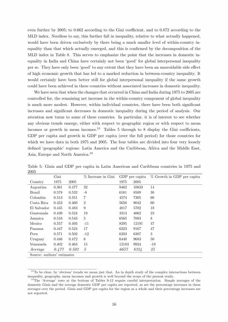
incomes or growth in mean incomes.18 Tables 5 through to 8 display the Gini coeffi cients,

GDP per capita and growth in GDP per capita (over the full period) for those countries for

which we have data in both 1975 and 2005. The four tables are divided into four very loosely

defined ‘geographic’regions: Latin America and the Caribbean, Africa and the Middle East,

Asia, Europe and North America.19

Table 5: Ginis and GDP per capita in Latin American and Caribbean countries in 1975 and2005

Gini % Increase in Gini GDP per capita % Growth in GDP per capitaCountry 1975 2005 1975 2005Argentina 0.361 0.477 32 9462 10833 14Brazil 0.578 0.532 -8 6161 8509 38Colombia 0.513 0.551 7 4574 7305 60Costa Rica 0.453 0.460 2 5650 9042 60El Salvador 0.445 0.483 9 4817 5702 18Guatemala 0.439 0.524 19 3313 4062 23Jamaica 0.516 0.543 5 6565 7083 8Mexico 0.557 0.493 -11 8295 12191 47Panama 0.447 0.524 17 6223 9167 47Peru 0.571 0.502 -12 6203 6387 3Uruguay 0.446 0.472 6 6440 9683 50Venezuela 0.402 0.463 15 12183 9924 -19Average 0.477 0.502 5 6657 8324 25Source: authors’estimates

18To be clear, by ‘obvious’trends we mean just that. An in depth study of the complex interactions betweeninequality, geography, mean incomes and growth is well beyond the scope of the present study.19The ‘Average’ rows at the bottom of Tables 9-12 require careful interpretation. Simple averages of the

domestic Ginis and the average domestic GDP per capita are reported, as are the percentage increases in theseaverages over the period. Ginis and GDP per capita for the region as a whole and their percentage increases arenot reported.

16

Table 6: Ginis and GDP per capita in African and Middle Eastern countries in 1975 and 2005Gini % Increase in Gini GDP per capita % Growth in GDP per capita

Country 1975 2005 1975 2005Cote d’Ivoire 0.529 0.500 -5 2686 1666 -38Egypt 0.435 0.378 -13 1687 4491 166Malawi 0.519 0.444 -14 639 645 1Nigeria 0.498 0.489 -2 1574 1750 11Tunisia 0.496 0.462 -7 3387 7182 112Zambia 0.519 0.557 7 1773 1158 -35Iran 0.560 0.439 -22 9759 9228 -5Israel 0.360 0.408 13 13984 23340 67Jordan 0.406 0.444 9 2277 4334 90Turkey 0.470 0.455 -3 5907 11465 94Average 0.479 0.458 -5 4367 6526 49Source: authors’estimates

Table 7: Ginis and GDP per capita in Asian countries in 1975 and 2005Gini % Increase in Gini GDP per capita % Growth in GDP per capita

Country 1975 2005 1975 2005Australia 0.317 0.275 -13 18183 32523 79China 0.279 0.485 74 409 4115 906Indonesia 0.427 0.448 5 1016 3102 205Republic of Korea 0.390 0.319 -18 4284 22783 432Philippines 0.452 0.467 3 2424 3051 26Thailand 0.417 0.444 6 1694 6675 294India 0.402 0.509 27 849 2209 160Nepal 0.510 0.521 2 570 954 67Pakistan 0.350 0.369 5 1065 2145 101Sri Lanka 0.389 0.456 17 1313 3550 170Average 0.393 0.429 9 3181 8111 155Source: authors’estimates

Some obvious trends do emerge from Tables 9 to 12. As expected, domestic inequality has

been generally rising between 1975 and 2005. Africa and the Middle East is the only one of

our loosely defined regions in which the average country from our sample has seen a decline

in inequality. Within each region, there is considerable variation with respect to levels of, and

changes in, inequality. For example, in Europe, Bulgaria’s Gini has increased by 87 per cent,

while Greece’s has fallen by 18 per cent; in Latin America, Argentina’s Gini has increased by 32

per cent, while Brazil’s has fallen by 8 per cent; in the Middle East, Israel’s Gini has increased

by 13 per cent, while Iran’s has decreased by 22 per cent and in Asia, China’s Gini has increased

by 74 per cent, while Korea’s has decreased 18 per cent. The latter comparison is an interesting

one. China and Korea have both been extraordinarily successful with respect to growth in

mean incomes over the period studied, yet have had very different experiences with respect to

changes in domestic inequality. An in-depth study of the relationships between mean incomes

17

Table 8: Ginis and GDP per capita in European and North American countries in 1975 and2005

Gini % Increase in Gini GDP per capita % Growth in GDP per capitaCountry 1975 2005 1975 2005Austria 0.292 0.293 0 17555 33626 92Belgium 0.265 0.286 8 17898 32189 80Bulgaria 0.169 0.316 87 5921 9809 66Canada 0.325 0.330 2 20374 35033 72Denmark 0.272 0.237 -13 18390 33193 80Finland 0.222 0.275 24 15501 30708 98France 0.345 0.310 -10 17550 29453 68Germany 0.319 0.306 -4 17592 31115 77Greece 0.398 0.326 -18 14809 24348 64Hungary 0.224 0.302 35 9628 16975 76Ireland 0.299 0.326 9 11339 38896 243Italy 0.383 0.361 -6 15406 28280 84Netherlands 0.276 0.295 7 20030 35104 75Norway 0.313 0.290 -7 21411 47626 122Portugal 0.372 0.363 -2 10057 21369 112Spain 0.324 0.372 15 14693 27392 86Sweden 0.235 0.254 8 19329 32703 69Switzerland 0.336 0.309 -8 29274 36964 26UK 0.233 0.361 55 16625 32958 98USA 0.357 0.411 15 22396 42516 90Average 0.298 0.316 6 16789 31013 85Source: authors’estimates

and inequality and growth in mean incomes and changes in inequality are not our intention.

Nevertheless, some interesting correlations do emerge from the data in Tables 9 to 12. These

are displayed in Table 9.

Table 9: Correlations between inequality, GDP per capita and growthCorrelations

1975 Gini & 2005 Gini & % Inc in Gini &GDP per cap GDP per cap Growth in GDP per cap

Latin America & Caribbean -0.306 -0.435 -0.215Africa & Middle East -0.357 -0.487 0.028Asia -0.376 -0.867 0.705Europe & North America 0.316 -0.036 0.018Total Sample -0.564 -0.801 0.356Source: authors’estimates

Overall, higher Gini coeffi cients appear quite strongly negatively correlated with levels of

GDP per capita, and the strength of the correlation is higher in 2005 than it was in 1975.

This pattern holds in each of our individual regions, apart from Europe and North America.

Overall, and somewhat in contrast, there is a modest positive correlation between the increase

in Gini coeffi cients and growth in GDP per capita. However, this pattern is not consistent across

regions and is mainly driven by Asia, in which there is a strong positive correlation. In fact,

18

this correlation disappears completely when China is omitted.20 Omitting China has relatively

little impact, however, on the correlations between Gini and GDP per capita levels; without

China the overall correlations for 1975 and for 2005 become -0.607 and -0.798 respectively.

7 Sensitivity analysis

We are aware of some of the potential sources of error in our estimates of global inequality,

including sampling error, measurement error and, as discussed by Anand and Segal (2008),

assuming a single PPP price level for each country. There is also the issue of the extent to

which assuming equal incomes within country-quantiles is likely to bias the inequality measures

downwards.

Anand and Segal (2008:90) have argued that ‘Sensitivity analysis should be undertaken to

assess the possible impact of these errors and assumptions, even if there is insuffi cient informa-

tion to estimate statistical confidence intervals...’They also illustrate in some detail why ‘The

standard errors estimated in the literature do not address these concerns.’We broadly agree

with Anand and Segal (2008). With respect to the diffi culties involved in estimating statistical

confidence intervals, we would perhaps even go as far as to argue that such a task is impossible.

There is simply too much uncertainty regarding the sizes and directions of some of the biases.

We will discuss some of the issues in turn and then consider their possible net impact.

7.1 Sampling error and bias

There are well-established techniques for estimating the standard errors arising from a sample

not being representative of the population under study. The diffi culty in the present context, as

pointed out by Anand and Segal (2008), is that we are not dealing with a random sample of the

global population. Rather we are dealing with a constructed sample, based on many different

national surveys, each with their own sampling variance. Estimating the sampling variance of

the resulting distribution is a diffi cult problem and a solution is not easily apparent.

A related issue is the extent to which our results are likely to suffer from sample selection

bias. Given the nature of household surveys, one might expect this to impart a downward

bias on our estimates, since it is rare for very high earners to be surveyed. However, we make

this conjecture somewhat tentatively and without a method for estimating the extent of this

potential bias. Moreover, any such bias needs to be considered in tandem with possible biases

arising from measurement error, as discussed next.

7.2 Measurement error

Measurement error is likely to arise from a number of sources, notably the quantile share data

from the various surveys and the GDP data measured in US$ PPP. Indeed measurement error

in the latter might itself arise from either the raw GDP calculations or the estimation of the

PPP conversion rates. Measurement error in the population data is a further possibility.

Anand and Segal (2008) argue that since the responses from those who are surveyed are

likely to be noisy, this would bias the variance of the responses upwards which might cause20 Indeed it becomes slightly negative, falling to -0.031 overall and to -0.280 in Asia.

19

measured inequality to be overstated. This is a reasonable argument. However, as Anand and

Segal (2008) also point out, surveys are also likely to suffer from underreporting of the incomes

of the rich and from undersampling of both the richest and the poorest. These dynamics would

be expected to bias inequality in the opposite direction.

Now, if the GDP data are biased upwards (respectively, downwards) for low-income coun-

tries, or downwards (respectively, upwards) for high-income countries, measured global inequal-

ity will be biased downwards (respectively, upwards), due to the resulting impact on the between-

country component of inequality.

If population sizes are biased upwards (respectively, downwards) in lower-income countries,

or downwards (respectively, upwards) in higher-income countries, this will tend to bias measured

global inequality upwards (respectively, downwards), due to the resulting impact on both the

between-country and within-country components of inequality. Unfortunately, however, the

direction and size of biases resulting from measurement error in the GDP data and of country

population sizes are very diffi cult to predict. Overall, given the multitude of surveys and the

various uncertainties involved, it is unfortunately not at all clear what even the direction of the

net bias due to measurement error should be expected to be, let alone its size. This is certainly

an area for future research enquiry.

7.3 Assuming a single PPP price level for each country

Further biases are likely due to the necessary evil of assuming a single PPP price level for each

country-year. This issue has been discussed by Aten and Heston (2010) and Anand and Segal

(2008). In short, if prices faced by individuals are positively correlated with incomes, as is

often the case, the assumption of a single PPP price level will tend to bias measured inequality

upwards.21 On the other hand, economies of scale tend to favour the better off, who are more

likely to be able to buy in bulk. This may result in a negative correlation between prices and

incomes and a downward bias on measured inequality. The overall direction of the net bias

even at a given country-level is diffi cult to predict; estimating the overall effect of such biases

globally appears an almost insurmountable task.

7.4 Assuming equal incomes within quantiles

As we have discussed, in this source of error at least, there is no doubt about the direction

of the bias. Assuming equal incomes within country-quantiles certainly biases our inequality

measures downwards and indeed, ignoring the various other sources of bias discussed above, we

might consider our various inequality estimates to be lower bounds.

Anand and Segal (2008:88) have suggested that studies which take our approach should

construct an upper bound for within-country inequality, by considering how high inequality

would be if the distribution within income intervals were assumed to be maximally unequal.

We agree that this is a nice idea. However, it is a more challenging problem that it might, at

first sight, appear. The main diffi culty stems from the fact that we do not, in general, know

the upper- and lower-income bounds within each quantile. So, for example, inequality would

increase if the income of the poorest individual in the second quantile decreases as far as is21 It is well known that incomes are often higher in expensive regions.

20

possible, whilst remaining in the second quantile. Inequality will also increase if the income of

the richest person in the poorest quantile increases as far as is possible, while remaining in the

first quantile. Unfortunately, however, we do not know where the cut-off point between the two

quantiles is.

If there were just two quantiles, it might be relatively straightforward to evaluate the optimal

(counterintuitively, with respect to maximizing inequality) cut-off point between the quantiles

but the complexity of the problem increases as the number of quantiles increases. Consider

the following. As the upper bound to the first quantile decreases, this tends to decrease the

amount of inequality that can arise within the first quantile and increase the inequality that

can arise within the second quantile. However, with more than two quantiles, we also need to

choose a cut-off point that bounds the top of the second quantile from the bottom of the third

quantile. The truly optimal bound for the top of the first quantile (with respect to maximizing

inequality) can then be expected to depend on where the optimal upper bound to the second

quantile lies - and so on. A solution to this problem is not readily apparent to us and it perhaps

represents an interesting topic for future research.

8 Discussion

Our overall estimates of global inequality levels lie broadly in the same ball park as those of

previous studies. For example, Dowrick and Akmal (2005) reported Ginis of 0.698 in 1980 and

0.711 in 1993, Sala-i-Martin (2006) found Ginis of 0.660 in 1980 and 0.637 in 2000, Bhalla (2002)

reported Ginis of 0.686 in 1980 and 0.651 in 2000, Bourguignon and Morrisson (2002) found a

Gini of 0.657 in both 1980 and 1992 and Milanovic (2005) reported Ginis of 0.622 in 1988 and

0.641 in 1998.

Our estimates lie towards the upper end of the existing literature, closest to Dowrick and

Akmal (2005). This is likely to be partially related to the manner in which we have adjusted

for data which are reported as consumption quantiles rather than income quantiles. As we have

discussed, this imparts an (intentional) upward impact on our global inequality measurements.

Our analysis of the impact of China on global interpersonal inequality is consistent with

that of Sala-i-Martin (2006), who found that without China, global inequality would have risen

from 0.620 to 0.648 from 1970 to 2000, whereas in fact it actually decreased.

Our analysis of trends in within-country and between-country inequality and of the impact

of India and China seem at least partially consistent with that of Bourguignon and Morrisson

(2002). They found that between 1970-92, global income inequality, as measured by the MLD

index, increased slightly from 0.823 to 0.827. Whilst we found that global income inequality

decreased between 1975 and 1995, our within-country and between-country components moved

in the same directions as theirs. (Their within-country component increased from 0.304 to

0.332, while their between-country component decreased from 0.518 to 0.495).

Bourguignon and Morrisson (2002:738) also found that ‘...the relatively poor growth per-

formances of China and India until late in the 20th century’was one of the main ‘disequalizing

forces’while ‘China’s outstanding growth performance in the last decade or two of the period’

was one of the main ‘equalizing forces.’Whilst we consider a much shorter period of analysis

(which starts much later but also finishes later), our results as to the impact of China and India

21

are consistent with theirs.

There are also some notable points of divergence in our results. For example, Milanovic

(2002) found that inequality, as measured by the Gini index, increased from 0.63 in 1988 to

0.66 in 1993. Moreover, this increase was driven more by differences in mean incomes between

countries than by inequalities within countries. Although we do not consider these exact years,

these results do seem somewhat at odds with our findings for 1985-95, especially with respect to

the trends in within-country and between-country inequality; as discussed at length in Section

3, we find that within-country inequality increased considerably over this period, while between-

country inequality decreased substantially.

9 Conclusions

Using the most up-to-date and complete database of worldwide distributional data presently

available, we have estimated global interpersonal inequality levels and their trends during the

period from 1975 to 2005. This is the first study to provide a comprehensive picture of global

inequality levels prior to the financial crisis of 2007-08.

As in previous studies, the global inequality figures estimated in this paper represent very

high levels indeed. This is especially so in light of the fact that our figures might be considered,

as we have discussed, to be lower bounds of the true values. Generally speaking, we live today in

a very unequal world. Global inequality figures are much higher than domestic levels in even the

most unequal countries of Latin America and sub-Saharan Africa. The dynamic which causes

this is clear from our decomposition of global inequality into within-country and between-

country components. The latter component is still the dominant factor in global inequality.

This is due to the dramatic growth in China and India that accompanied dramatic increases in

inequality in those countries, and which in turn resulted in a net decrease in global inequality.

Strong but above all, more ’inclusive’growth in developing countries, especially populous ones,

remains a potent tool for reducing global interpersonal inequality.

However, the general trend towards increasing domestic inequality should be a matter for

concern, not just for nation states, but also for those concerned with global equity and stability.

If current upward patterns of inequality continue in large emerging markets such as China

and India, with dramatic growth but also large increases in domestic inequality, in not too

many years time this will lead to increases in both the within-country and between-country

components of global inequality.

A major challenge for both future research and for policy makers in the years ahead will

be to find ways of achieving strong growth without allowing inequality to spiral to dangerous

levels. It may be instructive to learn from the experiences of countries such as the Republic of

Korea which have somehow managed to achieve this.

Finally, it is worth reflecting on the fact that there are other dimensions to inequality

than the income-based focus in this study and others we have referred to. Some are likely to

be strongly correlated with income but others perhaps less so. Bourguignon and Morrisson

(2002:728), for example, have found that ‘health disparities are probably not much larger today

than they were in the early 19th century...’, despite dramatic increases in income inequality. This

may or may not be the case across other important dimensions of wellbeing such as education,

22

easy access to clean water and so on. Greater knowledge in these domains would clearly be of

significant value.

References

[1] Acemoglu, D. (2011), ‘Thoughts on inequality and the financial crisis,’paper presented at

the AEA meeting, Denver, 7 January, [http://economics.mit.edu/files/6348], accessed 19

February 2013.

[2] Alesina, A. and Perotti, R. (1996), ‘Income distribution, political instability, and invest-

ment,’European Economic Review 40, 1203-1228.

[3] Amiel, Y. and Cowell, F. (1992), ‘Measurement of Income Inequality: Experimental Test

by Questionnaire,’Journal of Public Economics 47, 3-26.

[4] Amiel, Y. and Cowell, F. (1997). Income Transformation and Income Inequality, Distribu-

tional Analysis Discussion Paper 24, STICERD, London School of Economics.

[5] Anand, S. (1983), Inequality and Poverty in Malysia: Measurement and Decomposition.

Oxford and New York: Oxford University Press.

[6] Anand, S.and Segal, P. (2008), ‘What do we know about global income inequality?’Journal

of Economic Literature 46, 57-94.

[7] Arneson, R. (1989), ‘Equality of opportunity for welfare,’Philos. Stud. 56, 77—93.

[8] Aristotle (1954) Rhetoric. Book II, Chapter 2, 1379a. Translation of Rhys Roberts. Com-

piled by Lee Honeycult, web edition at www.public.iastate.edu

[9] Arellano, M. and Bond, S. (1991), ‘Some Tests of Specification for Panel Data: Montecarlo

Evidence and an Application to Employment Equations,’Review of Economic Studies 58,

277-297.

[10] Aten, B and Heston, A. (2010), ‘Use of Country Purchasing Power Parities for International

Comparisons of Poverty Levels: Potential and Limitations,’in Debates in the Measurement

of Global Poverty, ed. S. Anand, P. Segal and J. Stiglitz. Oxford and New York: Oxford

University Press.

[11] Atkinson and Brandolini (2010), ‘On analysing the world distribution of income,’ The

World Bank Economic Review 24, 1-37.

[12] Atkinson and Morelli (2011), ‘Economic crises and inequality,’UNDP Human Development

Research Paper 2011/06.

[13] Banerjee, A. and Duflo, E. (2003), ‘Inequality And Growth: What Can The Data Say?,’

Journal of Economic Growth 8, 267-299.

[14] Barro, R. (2000), ‘Inequality and Growth in a Panel of Countries,’Journal of Economic

Growth 5, 5-32.

23

[15] Benabou, R. (1996), ‘Inequality and Growth,’in Ben S. Bernanke and Julio J. Rotemberg,

eds., NBER macroeconomics annual 1996. Cambridge, MA: MIT Press, pp. 11-74.

[16] Berg, A. G. and Ostry, J. D. (2011) ‘Inequality and unsustainable

growth: Two sides of the same coin’, IMF Staff Discussion Note, 8 April,

[http://www.imf.org/external/pubs/ft/sdn/2011/sdn1108.pdf], accessed 19 February

2013.

[17] Bhalla, S. (2002), Imagine there’s no country: Poverty, Inequality and Growth in the Era

of Globalization. Washington, D.C.: Institute for International Economics.

[18] Boltho, A. and Toniolo, G. (1999), ‘The Assessment: The Twentieth Century-

Achievements, Failures, Lessons,’Oxford Review of Economic Policy 15, 1-17.

[19] Bordo, M. and Meissner, C. (2012), ‘Does inequality lead to a financial crisis?’ Journal of

International Money and Finance 31, 2147-2161.

[20] Bourguignon, F. (1979) ’Decomposable Income Inequality Measures’, Econometrica , Vol.

47, No. 4, pp. 901-920

[21] Bourguignon, F. and Morrisson, C. (2002), ‘Inequality among World Citizens: 1820-1992,’

American Economic Review 92, 727-744.

[22] Caselli, F., Esquivel, G. and Lefort, F. (1996), ‘Reopening the Convergence Debate: A

New Look at Cross-Country Growth Empirics,’Journal of Economic Growth 1, 363-389.

[23] Chotikapanich, D., Valenzuela, R. and Prasado Rao, D. (1997), ‘Global and Regional

Inequality in the Distribution of Income: Estimation with Limited and Incomplete Data,’

Empirical Economics 22, 533-546.

[24] Cohen, G.A. (1989), ‘On the currency of egalitarian justice. Ethics 99, 906—944.’

[25] Cornia, G. A. and Kiiski, S. (2001), ‘Trends in Income Distribution in the Post-World War

II Period: Evidence and Interpretation,’UNU-WIDER Discussion Paper No. 2001/89.

[26] Deininger, K. and Squire, L. (1996), ‘A New Data Set Measuring Income Inequality,’World

Bank Economic Review 10, 565-591.

[27] Dickhanov, Y. and Ward, M. (2002), ‘Evolution of the Global Distribution of Income, 1979-

1999,’Paper presented at the 5th Conference on Globalization, Growth and (In)Equality

held in Warwick, UK, March 15-17, 2002.

[28] Dowrick, S. and Akmal, M. (2005), ‘Contradictory Trends in Global Income Inequality: A

Tale of Two Biases,’Review of Income and Wealth 51, 201-229.

[29] Dowrick, S. and Quiggin, J. (1997), ‘True Measures of GDP and Convergence,’American

Economic Review 87, 41-64.

[30] Dworkin, R. (1981a), ‘What is equality? Part one: Equality of welfare,’ Philosophy &

Public Affairs 10, 185-246.

24

[31] Dworkin, R. (1981b), ‘What is equality? Part two: Equality of resources,’Philosophy &

Public Affairs 10, 283-345.

[32] Firebaugh, G. (1999), ‘Empirics of World Income Inequality,’American Journal of Sociol-

ogy 104, 1597-1630.

[33] Firebaugh, G. (2003), The New Geography of Global Income Inequality. Cambridge and

London: Harvard University Press.

[34] Fleurbaey, M. (2008), Fairness, Responsibility, and Welfare. Oxford University Press, Lon-

don.

[35] Forbes, K. (2000), ‘A Reassessment of the Relationship between Inequality and Growth,’

American Economic Review 90, 869-887.

[36] Holtz-Eakin, D., Newey, W., & Rosen, H. S. (1988), ‘Estimating vector autoregressions

with panel data,’Econometrica 56, 1371-1395.

[37] Islam, N. (1995), ‘Growth Empirics: A Panel Data Approach,’Quarterly Journal of Eco-

nomics 110, 1127—70.

[38] Kelly, M. (2000), ‘Inequality and Crime,’Review of Economics and Statistics 82, 530-539.

[39] Kolm, S. (1976). Unequal Inequalities I and II, Journal of Economic Theory, 12, 416-442,

and 13, 82-111.

[40] Korzeniewicz, R. and Moran, T. (1997), ‘World-Economic Trends in the Distribution of

Income, 1965-1992,’American Journal of Sociology 102, 1000-1039.

[41] Kuznets, S (1955), ‘Economic Growth and Income Inequality,’American Economic Review,

45(1), pp. 1-28.

[42] Lewis, W. A. (1954), ’Economic Development with Unlimited Supplies of Labour’, The

Manchester School, 22: 139—191

[43] Melchior, A., Telle, K. and Wiig, H. (2000), ‘Globalization and Inequality: World Income

Distribution and Living Standards, 1960-1998,’Royal Norwegian Ministry of Foreign Af-

fairs, Studies on Foreign Policy Issues Report, No. 6B.

[44] Milanovic, B. (2002), ‘True World Income Distribution, 1998 and 1993: First Calculation

Based on Household Surveys Alone,’Economic Journal 112, 51-92.

[45] Milanovic, B. (2005), Worlds Apart: Measuring International and Global Inequality.

Princeton and Oxford: Princeton University Press.

[46] Plato (1901) The Republic. Chapter 4 on wealth, poverty and virtue, No. 422. Translation

of Benjamin Jowett, web edition at www.mdx.ac.uk, Stephanus page numbers used

[47] Rajan, R G, 2010, Fault lines: How hidden fractures still threaten the world economy,

Princeton University Press, Princeton.

25

[48] Rawls, J.: A Theory of Justice. Harvard University Press, Cambridge (1971).

[49] Richardson, D., (1995), ‘Income inequality and trade: how to think, what to conclude,’

Journal of Economic Perspectives 9, 33-56.

[50] Roemer, J.E. 1993. ‘A pragmatic theory of responsibility for the egalitarian planner,’Philos-

phy & Public Affairs 22, 146-166.

[51] Roemer, J. E. (1998): Equality of Opportunity, (Cambridge, MA: Harvard University

Press).

[52] Sala-i-Martin, X. (2006), ‘The World Distribution of Income: Falling Poverty

and...Convergence, Period,’Quarterly Journal of Economics 121, 351-397.

[53] Schultz, P. (1998), ‘Inequality in the Distribution of Personal Income in the World: How

it is Changing and Why,’Journal of Population Economics 11, 307-344.

[54] Solow, R. (1956) ’A Contribution to the Theory of Economic Growth’, The Quarterly

Journal of Economics (1956) 70 (1): 65-94

[55] Joseph E. Stiglitz (2012), ‘Macroeconomic Fluctuations, Inequality, and Human Develop-

ment,’Journal of Human Development and Capabilities 13, 31-58.

[56] UNDP (1999), Human Development Report, 1999. New York and Oxford: Oxford Univer-

sity Press.

[57] Wilkinson, R. and Pickett, K. (2006), ‘Income inequality and population health: A review

and explanation of the evidence,’Social Science & Medicine 62, 1768—1784.

[58] Williamson, J. (1999). ‘Globalization and inequality then and now: the late 19th and late

20th centuries compared’, National Bureau of Economic Research Working Paper no. 5491,

Cambridge, Mass.

[59] Wood, A. (1995). ‘How trade hurt unskilled workers’, Journal of Economic Perspectives 9,

57-80.

[60] World Bank (2008), ‘Global Purchasing Power Parities and Real Ex-

penditures: 2005 International Comparison Program,’ available online at

[http://siteresources.worldbank.org/ICPINT/Resources/icp-final.pdf], accessed 24 Febru-

ary 2013.

[61] You, J-S and Khagram, S. (2005), ‘A Comparative Study of Inequality and Corruption,’

American Sociological Review 70, 136-157.

26

10 Appendix

Table 10: Countries covered in 1975

Argentina, Australia, Austria, Barbados, Belgium, Botswana, Brazil, Bulgaria,Canada, China, Colombia, Costa Rica, Cote d’Ivoire, Denmark, Ecuador, Egypt,El Salvador, Fiji, Finland, France, Gabon, Germany, Greece, Guatemala,Hong Kong, Hungary, India, Indonesia, Iran, Ireland, Israel, Italy,Jamaica, Japan, Jordan, Kenya, Republic of Korea, Malawi, Malaysia,Mexico, Morocco, Nepal, Netherlands, New Zealand, Nigeria, Norway,Pakistan, Panama, Peru, Philippines, Portugal, Spain, Sri Lanka, Sweden,Switzerland, Thailand, Trinidad & Tobago, Tunisia, Turkey, UK, USA,Uruguay, Venezuela, Zambia

Table 11: Countries covered in 1985

Algeria, Argentina, Australia, Austria, Bahamas, Bangladesh, Belarus,Belgium, Bolivia, Botswana, Brazil, Bulgaria, Canada, Chile, China,Colombia, Costa Rica, Cote d’Ivoire, Czech Republic, Denmark,Dominican Republic, Ecuador, El Salvador, Ethiopia, Finland, France,Germany, Ghana, Greece, Guatemala, Honduras, Hong Kong, Hungary,India, Indonesia, Ireland, Israel, Italy, Jamaica, Japan, Jordan,Kazakhstan, Republic of Korea, Kyrgyz Republic, Latvia, Lesotho,Lithuania, Luxembourg, Madagascar, Malawi, Malaysia, Mali,Mauritania, Mexico, Moldova, Morocco, Nepal, Netherlands,New Zealand, Nigeria, Norway, Pakistan, Panama, Paraguay, Peru,Philippines, Poland, Portugal, Romania, Russia, Rwanda, Sierra Leone,Slovak Republic, Slovenia, Spain, Sri Lanka, Sweden, Switzerland,Thailand, Trinidad & Tobago, Tunisia, Turkey, Turkmenistan,Uganda, Ukraine, UK, USA, Uruguay, Uzbekistan, Venezuela

27

Table 12: Countries covered in 1995

Albania, Algeria, Argentina, Armenia, Australia, Austria, Bahamas, Bangladesh,Belarus, Belgium, Bolivia, Brazil, Bulgaria, Burkina Faso, Burundi, Cambodia,Cameroon, Canada, Central African Republic, Chile, China, Colombia, Costa Rica,Cote d’Ivoire, Croatia, Czech Republic, Denmark, Djibouti, Dominican Republic,Ecuador, Egypt, El Salvador, Estonia, Ethiopia, Fiji, Finland, France, Gambia,Georgia, Germany, Ghana, Greece, Guatemala, Guinea, Guinea-Bissau, Guyana,Honduras, Hong Kong, Hungary, India, Indonesia, Iran, Ireland, Israel, Italy,Jamaica, Japan, Jordan, Kazakhstan, Kenya, Republic of Korea, Kyrgyz Republic,Lao, Latvia, Lesotho, Lithuania, Luxembourg, Macedonia, Madagascar, Malawi,Malaysia, Mali, Mauritania, Mexico, Moldova, Mongolia, Morocco, Mozambique,Namibia, Nepal, Netherlands, New Zealand, Nicaragua, Niger, Nigeria, Norway,Pakistan, Panama, Papua New Guinea, Paraguay, Peru, Philippines, Poland, Portugal,Romania, Russia, Rwanda, Senegal, Serbia & Montenegro, Slovak Republic,Slovenia, South Africa, Spain, Sri Lanka, Suriname, Swaziland, Sweden, Switzerland,Tajikistan, Tanzania, Thailand, Trinidad & Tobago, Tunisia, Turkey, Turkmenistan,Uganda, Ukraine, UK, USA, Uruguay, Uzbekistan, Venezuela, Vietnam, Yemen,Zambia

Table 13: Countries covered in 2005

Albania, Argentina, Armenia, Australia, Austria, Azerbaijan, Bahamas, Bangladesh,Belarus, Belgium, Bolivia, Bosnia and Herzegovina, Brazil, Bulgaria, Burkina Faso,Cambodia, Cameroon, Canada, Chile, China, Colombia, Costa Rica, Cote d’Ivoire,Croatia, Czech Republic, Denmark, Dominican Republic, Ecuador, Egypt,El Salvador, Estonia, Ethiopia, Finland, France, Georgia, Germany, Greece,Guatemala, Guinea, Haiti, Honduras, Hungary, India, Indonesia, Iran, Ireland,Israel, Italy, Jamaica, Jordan, Kazakhstan, Republic of Korea, Kyrgyz Republic,Lao, Latvia, Lithuania, Luxembourg, Macedonia, Madagascar, Malawi, Mali,Mauritania, Mexico, Mongolia, Mozambique, Nepal, Netherlands, Nicaragua,Nigeria, Norway, Pakistan, Panama, Paraguay, Peru, Philippines, Poland, Portugal,Romania, Russia, Senegal, Serbia and Montenegro, Slovak Republic, Slovenia,South Africa, Spain, Sri Lanka, Swaziland, Sweden, Switzerland, Tajikistan,Tanzania, Thailand, Tunisia, Turkey, Uganda, Ukraine, UK, USA, Uruguay,Uzbekistan, Venezuela, Vietnam, Yemen, Zambia

28