NBER WORKING PAPER SERIES

WHY TIE A PRODUCT CONSUMERS DO NOT USE?

Dennis W. CarltonJoshua S. Gans

Michael Waldman

Working Paper 13339http://www.nber.org/papers/w13339

NATIONAL BUREAU OF ECONOMIC RESEARCH1050 Massachusetts Avenue

Cambridge, MA 02138August 2007

We thank seminar participants at the University of Melbourne, Thomas Barnett, Justin Johnson andStephen King for helpful discussions and the Intellectual Property Research Institute of Australia andthe Australian Research Council for financial support. Carlton served as expert adverse to Microsoftand is currently serving as the Deputy Assistant Attorney General at the Antitrust Divisiion, Departmentof Justice. The views in this paper reflect those of the authors and not necessarily those of the Departmentof Justice, or any organization the authors have been involved with, or the National Bureau of EconomicResearch.

© 2007 by Dennis W. Carlton, Joshua S. Gans, and Michael Waldman. All rights reserved. Short sectionsof text, not to exceed two paragraphs, may be quoted without explicit permission provided that fullcredit, including © notice, is given to the source.

Why Tie A Product Consumers Do Not Use?Dennis W. Carlton, Joshua S. Gans, and Michael WaldmanNBER Working Paper No. 13339August 2007JEL No. L10,L12,L4,L40,L41,L42

ABSTRACT

This paper provides a new explanation for tying that is not based on any of the standard explanations-- efficiency, price discrimination, and exclusion. Our analysis shows how a monopolist sometimeshas an incentive to tie a complementary good to its monopolized good in order to transfer profits froma rival producer of the complementary product to the monopolist. This occurs even when consumers-- who have the option to use the monopolist's complementary good -- do not use it. The tie is profitablebecause it alters the subsequent pricing game between the monopolist and the rival in a manner favorableto the monopolist. We show that this form of tying is socially inefficient, but interestingly can ariseonly when the tie is socially efficient in the absence of the rival producer. We relate this inefficientform of tying to several actual examples and explore its antitrust implications.

Dennis W. CarltonGraduate School of BusinessThe University of Chicago5807 South WoodlawnChicago, IL 60637and NBERdennis.carlton@chicagogsb.edu

Joshua S. GansUniversity of Melbourne200 Leicester StreetCarlton VIC 3035AustraliaJ.Gans@mbs.edu

Michael WaldmanJohnson Graduate School of Management323 Sage HallCornell UniversityIthaca, NY 14853-6301mw46@cornell.edu

I. INTRODUCTION

Because of the attention paid to Microsoft’s behavior in the marketing of Windows and

its various applications programs, significant theoretical attention has recently been directed at

why a primary-good monopolist would tie a complementary good. Most of this recent literature

as well as earlier literature on the subject is based on either efficiency, price discrimination, or

exclusionary motivations for tying.1 This paper provides a new explanation for the monopoly

tying of complementary products that we believe matches a number of real-world cases better

than existing alternatives. In our explanation, tying alters the equilibrium to the subsequent

pricing game and in this way provides a way for the monopolist to capture some of the profits of

a rival producer of the complementary good.

The intuition for our results is that a monopolist who ties its complementary product to

its monopolized product is providing the consumer with a valuable option. The presence of that

option affects consumer willingness to pay for the rival’s complementary good and potentially

affects pricing, even when the consumer does in fact buy the rival’s good. More precisely, in a

situation in which, in the absence of a rival, tying would be efficient, a monopolist may tie

because, in the presence of the rival, the tie transfers profits from the sale of the rival’s

complementary good to the monopolist. The monopolist spends money to alter its “threat point”

in a Nash game so as to improve its profitability. Because the monopolist’s tied product is never

used, this behavior is inefficient, though profitable, and the behavior does not exclude the rival,

as in, for example, Whinston (1990) and Carlton and Waldman (2002).

To fix ideas with a simple example, consider Microsoft’s tying of Windows Media Player

(WMP) to Windows. Suppose Microsoft is the monopolist of Windows but that there is a better

media player available (as might be arguably the case with Quicktime or Real). Also, suppose

that an individual who consumes Windows and WMP derives a higher gross benefit if the two

goods are purchased as a tied product rather than purchased separately (either because of savings

on installation costs or because tying improves functionality). Suppose consumers are identical

and have a gross benefit of $15 for consuming Windows and WMP acquired separately, a gross

1 See Carlton and Waldman (2005) for a recent survey.

2

benefit of $25 for consuming Windows and the rival’s media player purchased separately, and

that the marginal cost for producing either type of media player is $2 (for simplicity assume the

cost of producing Windows is zero). Assuming Bertrand competition, no tying, and that the rival

producer captures all of the surplus associated with the rival’s superior complementary product,

consumers pay $12 for the rival’s media player, $13 for Windows, and do not install WMP. In

this outcome the rival’s per consumer profit equals $12-$2=$10, while Microsoft’s per consumer

profit equals $13-$0=$13.

Now suppose that, at the time of Windows production, Microsoft can costlessly

incorporate WMP and that an individual who consumes the tied product receives a gross benefit

of $20. The gross benefit of $20 exceeds the previous benefit from consuming the untied goods

because of, for example, savings on installation costs. Also, a consumer who purchases2 this tied

product can add the rival’s media player and receive, as before, a gross benefit of $25 because

the individual would employ the superior of the two available players. With the tie, as there is a

‘free option’ to use the bundled WMP, a consumer is only willing to pay $5 for the rival’s media

player. Assuming the surplus associated with the rival’s media player is still fully captured by

the rival, the price for the rival’s media player is $5 and the rival’s per consumer profit falls from

$10 to $5-$2=$3, while Microsoft’s price for the tied good is $20 and its per consumer profit

rises from $13 to $20-$2=$18. Note that the tying is socially inefficient since consumers do not

use WMP, but it is profitable for Microsoft since it changes the pricing game in a way that shifts

profits from the sale of the rival’s media player to Microsoft.3

In this paper, we consider a model that captures and extends the logic of the above

example. In our model, there is a monopolist of a primary product and a complementary product

that can be produced both by the monopolist and an alternative producer. Also, consumers have

a valuation only for systems, where a system consists of one primary unit and one or more

complementary units (although from the standpoint of consumption an individual uses only one

complementary unit even if he owns more than one). At the beginning of the period the

2 The example is simplified for tractability reasons. Obviously, if the complementary product comes in a base version for free but upgrades are costly, then it is the revenue from the upgrades that is relevant. The fact that the base product is free does not mean that there are no profits from tying because of the associated revenues from the upgrades and other features. In fact the base versions of Quicktime and Real Player are free but there are associated revenues from advanced features. 3 Note that should there be costs associated with the initial tie, this would (a) not necessarily remove Microsoft’s incentive to tie; and (b) increase the inefficiency associated with tying.

3

monopolist chooses whether or not to tie or sell individual products, where we assume ties are

reversible. A reversible tie means that a consumer who purchases a tied product from the

monopolist can add the alternative producer’s complementary product to their system although

they cannot return (say for a refund) the tied product. In effect, they have both but utilize one.

Although most of the literature focuses on irreversible ties, clearly, as in the case of Microsoft,

assuming ties are reversible is quite realistic.

What is interesting about this model is that its starting point is on a claim that Microsoft

relied upon in its various antitrust cases: that is, that there are efficiencies associated with

consuming its products as ties rather than acquired separately. Commentators had noted some

inconsistencies in the argument proferred by Microsoft. On the other side of the equation, are there plausible procompetitive explanations for these practices? Regarding its tying, Microsoft argued that its physical integration of Internet Explorer was no different in nature than its past integration of many other functionalities into Windows (and similar behavior by other software producers) which were done to make a better product. This argument seems plausible. Yet, for software, bundled sales are unnecessary to provide integrated functionality since code for upgraded features can be loaded separately onto a computer. Thus, any efficiency of bundled sales would seem to stem from reductions in consumers’ costs of acquiring and adding the features themselves and the software producer’s costs of distributing multiple products. Indeed, to the extent the efficiency relates to saving consumer costs, there is some tension between Microsoft’s claim that bundling is efficient and its claim, which I discuss below, that consumers can easily add Navigator. (Whinston, 2001, p.74)

What is more is that Microsoft believed “that its bundling would provide it with an advantage

over Netscape also seems evidence that it believed consumers’ perceived costs of adding

Navigator to be significant.” (Whinston, 2001, p.75) Our model embeds the increased

functionality and consumer cost savings that might accompany a tied product and shows how

this is linked to a tying strategy that would have been both profitable for Microsoft but also

inefficient from a social perspective.

We analyze a number of different cases. First, we analyze how the equilibrium depends

on whether consumers prefer the monopolist’s tied product to purchasing primary and

complementary units separately. Second, we analyze how the equilibrium depends on the

heterogeneity of consumer tastes. Third, we analyze how the equilibrium depends on whether

product quality is endogenous. For each of these cases we show how a tie can benefit the

monopolist even when the tied product is not ultimately used.

Our analysis does not fall into any of the existing theoretical categories for why a

monopolist of a primary good would tie a complementary product. Most previous explanations

4

for such tying are based on either efficiency, price discrimination, or exclusionary motivations.

As captured by the example above, in our argument the monopolist sometimes ties a product that

winds up not being used by consumers in equilibrium, in order to extract surplus from, but not

exclude, a rival producer. Specifically, the tying improves the monopolist’s position in the

pricing game that follows and, in this way, serves to shift profits from the rival to the

monopolist. Indeed, in contrast to standard results that rely on the exclusion or exit of a rival,

here it is the very profitability of the rival that drives strategic tying. Hence, a rival’s presence is

required for our results.

As discussed in more detail in the next section, one of the main points of our analysis is

that one of the main results in Whinston (1990) is not robust to the introduction of potential

efficiencies associated with tying. Whinston showed that, in the presence of a rival producer of a

complementary good, there is no return for a monopolist in tying as long as its primary good is

essential, i.e., required for all uses of the complementary good. But Whinston considered a

setting in which, in the absence of a rival, the monopolist has no incentive to tie. We instead

allow for tying to be efficient in the absence of the rival and show that, in combination with our

assumption that ties are reversible, this overturns Whinston’s result. That is, given a tie that is

efficient in the absence of a rival, in the presence of a rival, a reversible tie can be used to

increase profits even though the monopolist’s primary good is essential, where this type of tying

is frequently inefficient because, for example, consumers do not use the tied good in equilibrium.

The outline for the paper is as follows. Section II discusses how our analysis is related to

the previous literature on tying. Section III presents the main model and then analyzes an

illustrative example that demonstrates our argument in a setting characterized by identical

consumers who prefer the rival’s complementary good to the monopolist’s. Section IV

investigates the model considering both the one- and two-group cases, where our focus in the

case with two groups is what happens when the groups differ in terms of which complementary

good is preferred. Section V extends the analysis of Section IV by incorporating an R&D

expenditure that endogenously determines the size of the potential efficiency associated with

tying. Section VI discusses the antitrust implications of our analysis. In particular, we show that

while inefficient tying can arise in a competitive case, the incentives for such tying are stronger

under monopoly. Section VII presents concluding remarks.

5

II. RELATIONSHIP TO PREVIOUS LITERATURE

In most of the previous papers in which tying is used to disadvantage rival producers,

such as Whinston (1990), Choi and Stefanadis (2001), Carlton and Waldman (2002), and

Nalebuff (2004), the tying results either in the exit of existing rivals or blocks the entry of

potential rivals.4 For example, in Whinston’s model there is one market in which complementary

units are used in combination with primary units, while in a second market there is a demand for

complementary units by themselves. Whinston shows that, if there are economies of scale in the

production of the complementary good, then tying can be profitable because it causes rival

complementary-good producers to exit and thus allows the primary-good monopolist to

monopolize the market in which there is a demand for complementary units by themselves.

Carlton and Waldman (2002) consider a two-period setting in which there is an

incumbent monopoly producer of primary and complementary goods, where a rival producer can

enter the primary market only in the second period but the complementary market in either

period. In their model the alternative producer’s return to entering the primary market in the

second period is that this allows the firm to capture more of the surplus associated with its own

superior complementary product. Carlton and Waldman show that, given either entry costs or

complementary-good network externalities, the monopolist may tie in order to preserve its

monopoly position in the primary market in the second period. The logic is that tying can stop

entry into the complementary market by reducing its return and, in their model, the alternative

producer does not enter the primary market if it does not plan to enter the complementary

market.

The idea captured by the above cited papers that tying is used to exclude competition is

certaintly a plausible explanation for various important real-world cases. For example,

Microsoft’s tying of Internet Explorer with the Windows operating system does seem to have

eliminated Netscape’s Navigator as a serious competitor in the browser market and, to the extent

that Navigator posed a threat to the Windows monopoly as argued by the Justice Department,

also helped to preserve Microsoft’s monopoly in the operating systems market. However, there

are other important cases in which tying did not eliminate competition in the complementary-

4 Two exceptions are Carbajo, de Meza, and Seidman (1990) and Chen (1997). These papers are discussed in detail at the end of this section.

6

good market. For example, the more recent tying of WMP with Windows does not seem to have

eliminated all of the serious competition in media player applications programs. In fact, in

relation to Windows there are many similar ties. Instant messaging, movie and photo editing

programs, and more recently, computer search and security programs are all provided with

Windows despite the existence of seemingly superior independent alternatives that continue to

capture large market shares.5,6 This leads us to the question, can tying be used to disadvantage a

rival and improve monopoly profits even if there is no effect on the entry and exit decisions of

rival producers?

The analysis of our model yields that there are a number of cases in which the monopolist

impoves its own profitability and disadvantages a rival by tying even though there is no effect on

entry and exit decisions, although this typically happens only when in the absence of an

alternative producer consumers prefer the monopolist’s tied product to purchasing the

monopolist’s primary and complementary products separately.7 When consumers are indifferent

between these two options, tying is typically not profitable. The basic logic for this result was

first put forth in Whinston (1990). Whinston showed that tying cannot increase profits when the

monopolist’s primary good is essential, i.e., as is the case in our analysis the primary good is

required for all uses of the complementary good.8 The monopolist can ensure itself profits at

least as high as the profits associated with tying by selling the products separately, pricing the

complementary good at marginal cost, and pricing the primary good at the optimal bundle price

minus the complementary good’s marginal cost. Hence, tying in that case will typically not

increase profitability.

But when, in the absence of an alternative producer, consumers prefer the monopolist’s

tied good to purchasing the products individually, then there are a number of cases in which the

monopolist ties with no effect on entry and exit decisions but the result is increased monopoly

5 Indeed, the on-going tie of Internet Explorer has been met with new competition from Mozilla’s Firefox. 6 This applies to other Microsoft products too. For instance, this paper was written in Microsoft Word. It has a bundled equation editor but the equations here were written in Mathtype; a better, independently sold program. 7 If the model was restated in terms of the monopolist’s cost of producing the tied product relative to its cost of producing primary and complementary goods separately, the corresponding result is that the tie in our model can be profitable only when the monopolist’s cost of producing the tied product is strictly below its cost for producing the two goods separately. 8 This argument in some sense formalizes the earlier Chicago School argument that a monopolist would never tie a complementary good to its monopolized primary good because it can extract all of the potential profits through the

7

profitability and lower alternative producer profitability and social welfare. The simplest of these

cases, as in our example in the Introduction, is when consumers are identical, product qualities

are given exogenously, and all consumers prefer the alternative producer’s complementary good.

In this setting, there exists a range of parameterizations in which the monopolist ties, consumers

purchase the monopolist’s tied good and the alternative producer’s complementary good, and the

tie decreases social welfare because of the cost the monopolist incurs in producing

complementary units when the product is not used by consumers in equilibrium. We find a

similar result when we introduce consumer heterogeneity.

To understand why tying can be profitable, it is helpful to understand why Whinston’s

(1990) argument that shows no return to tying when the monopolist’s primary good is essential

does not apply.9 In Whinston’s argument the monopolist can sell its products individually and

price the goods in such a way that it ensures itself profits equal to tying profits. Hence, the

monopolist cannot increase its profits by tying. But here, because of the extra utility consumers

derive from the tied product when the alternative producer’s product is not purchased (when the

alternative producer’s product is purchased and used there is no extra utility associated with the

tie), the monopolist cannot ensure itself tying profits without in fact tying. The result is cases in

which the monopolist ties even though, in equilibrium, consumers purchase and use the

alternative producer’s complementary good so the consumers receive no benefit from owning the

monopolist’s complementary good. Clearly, in such a case the tie lowers social welfare because

of the direct production costs associated with the monopolist’s complementary good (and in the

case where the functionality of the tie is endogenous any R&D costs the monopolist incurs in

improving this functionality).10

Two other related papers on tying are Carbajo, De Meza, and Seidman (1990) and Chen

(1997). Both papers are similar to our paper in the sense that tying is used to increase profits by

pricing of the monopolized good. See, for example, Director and Levi (1956), Bowman (1957), Posner (1976), and Bork (1978). Also, see Ordover, Sykes, and Willig (1985) for a formal theoretical analysis related to Whinston’s. 9 Carlton and Waldman (2006) investigate a different setting in which a monopolist’s primary good is essential but Whinston’s argument does not apply. That argument focuses on durable goods and issues that arise in the presence of upgrades and switching costs. 10 This result depends on our assumption that ties are reversible, i.e., a consumer can add the alternative producer’s complementary product to a tied system consisting of the monopolist’s primary and complementary goods. Whinston assumes that ties are irreversible and it is the case that with irreversible ties the type of setting we investigate would never lead to inefficient tying. That is, the monopolist might tie even though the primary good is essential, but this would only occur when tying is efficient.

8

altering the outcome of the subsequent pricing game between the firms. For example, Carbajo,

De Meza, and Seidman consider a model with two independent products called A and B, where

product A is monopolized while B can be produced by the monopolist and a single alternative

producer. In the absence of tying, because the two firms produce identical products in the B

market and there is Bertrand competition between the firms, profits in the B market equal zero.

The main result is that, if the monopolist’s marginal cost for producing A is sufficiently high,

then tying allows the monopolist to increase its overall profitability. The basic logic is that tying

implicitly creates product differentiation in the B market and it is the introduction of this product

differentiation that serves to improve the monopolist’s profitability.

Although the two papers mentioned are similar to ours in the sense that tying is used to

affect the subsequent pricing game between the sellers, there are also important differences.

Most importantly, both papers focus on the case of independent products while we focus on the

monopoly tying of a complementary good where the monopolist’s primary good is essential. As

a result, the findings in these earlier papers are perfectly consistent with Whinston’s result

concerning essential primary products since, given independent products, any monopolized

product cannot be essential for the use of the other product. In contrast, as just discussed, one of

the main results of our paper is to show that Whinston’s result concerning essential primary

goods is not robust to the introduction of efficiencies such as increased functionality or reduced

installation costs associated with tying.

Finally, Farrell and Katz (2000) examine a market structure similar to ours with a single

monopoly provider of a primary good and one or more independent suppliers of a

complementary good. They consider various strategies the monopolist might engage in, most

notably, integration, R&D and exclusionary deals, in order to squeeze a rival producer of the

complementary good and appropriate greater profits. Our argument is similar to theirs in that we

also consider behavior that a monopoly producer of a primary good can employ in order to shift

profits from rivals to itself. However, our focus on the ability of a monopolist to accomplish this

through tying is not considered in Farrell and Katz’s analysis.11

11 Miao (2007) does consider the role tying might have in achieving the type of price squeeze discussed by Farrell and Katz. However, the set-up of that analysis is much different than ours and, in particular, Miao does not capture why a firm would tie a product that is not consumed in equilibrium.

9

III. MODEL AND EXAMPLE

Here we develop our model and assumptions and illustrate it using a specific example. A

general analysis follows in Section IV.

A. The Model

We consider a one-period setting characterized by a monopolist (M) and a single

alternative producer (A). The monopolist is the sole producer of what is referred to as the

primary good (P), while there is also a complementary good (C) that can be produced either by

the monopolist or the alternative producer. M has a constant marginal cost denoted cP (> 0), for

producing the primary good, while both M and A have a constant marginal cost cC (> 0), for

producing the complementary good. Further, there are no fixed costs of production for either

good and a unit of either type of good has a zero scrap value.

Primary and complementary goods are consumed together in what is referred to as

systems, where a system consists of either M’s primary and complementary products, M’s

primary good and A’s complementary good, or M’s primary good and both complementary

products. In the last case, although the consumers own both complementary goods, they use and,

thus, derive direct benefit from only one of the complementary products. Think of, for example,

the primary good as a computer operating system and the complementary good as a media player

applications program. The assumption that primary and complementary products are consumed

only together means that the monopolist’s primary good is essential in this model, i.e., it is

required for all uses of each of the complementary products.

At the beginning of the period the monopolist decides whether to offer the products

individually, sell a tied product consisting of its primary and complementary goods, or sell both

tied and individual products.12 In contrast to most of the previous theoretical literature on tying

used to disadvantage rival producers such as Whinston (1990), Choi and Stefanadis (2001),

Carlton and Waldman (2002), and Nalebuff (2004), we assume that ties are reversible. That is, a

consumer that purchases M’s tied product can add A’s complementary good to create a system

consisting of M’s primary good and both complementary goods. Especially in terms of Microsoft

12 See Adams and Yellen (1976) for an earlier analysis that allows the sale of both tied and individual products, although that analysis is in the setting of a pure monopoly seller.

10

whose behavior is the motivation for much of the recent attention to tying behavior, the

assumption of reversible ties is quite realistic.

There is a continuum of consumers on the unit interval. We make several assumptions on

the gross benefits derived by a consumer from various combinations of purchases. First, M’s

primary good is essential for all uses of the complementary good and vice versa. Hence,

consumer benefits are zero if they only consume one or the other of the primary and

complementary goods. Second, if a consumer uses the primary and complementary goods each

bought separately from M, their gross benefit is VM where we assume that MP CV c c> + . Third, if

P and C are purchased and consumed as a tied product from M, the consumer’s gross benefit

equals MV + Δ , Δ ≥ 0. Note, Δ = 0 means that consumers derive no direct added benefit from

consuming a tied product, while Δ > 0 means that a consumer with a system consisting of M’s

primary and complementary goods does derive a strictly positive added benefit from having

purchased and consumed a tied product. For example, if it costs a certain amount to install a

media player as a separate product then Δ represents those cost savings if the product is pre-

installed. However, Δ could also represent increased functionality made possible through the tie.

Notice that this means that, given there are no additional costs beyond P Cc c+ to producing a

tied product, when Δ > 0, tying would, in fact, be privately and socially desirable if no

alternative complementary product existed.13

What happens if the consumer purchases A’s complementary product? First, by

consuming a system consisting of M’s primary good and A’s complementary good, then the

consumer’s gross benefit equals VA. We also assume that A MV V> , i.e., in the absence of tying

A’s product is superior. Second, if the individual consumes a system consisting of M’s primary

good and both complementary goods (as may occur if M only sells a tied product), then the

complementary good that yields the highest gross benefit is used. For example, if a consumer

adds A’s complementary good to M’s tied product then the consumer’s gross benefit is given by

13 See Carlton and Perloff (2005) and Evans and Salinger (2005) for more extensive discussions of efficiency-based arguments for tying.

11

max{ , }M AV V+ Δ .14 Note, in this specification, even when Δ > 0, the tie is only valuable in

terms of gross benefits when the consumer uses the monopolist’s complementary good.

We assume Bertrand competition, but there is frequently a continuum of equilibria to the

pricing subgame. The difference between the equilibria is the division across the two sellers of

the surplus associated with A’s superior complementary product. Similar to the approaches taken

in Choi and Stefanadis (2001) and Carlton and Waldman (2002), we assume that λ of the surplus

is captured by the monopolist and (1–λ) is captured by the alternative producer, where

0 1λ≤ < .15

The timing of events in the model is as follows. First, the monopolist decides whether to

offer a tied product, individual products, or both tied and individual products. Second, the firms

simultaneously choose the prices for their products. Third, consumers make their purchase

decisions. Note that throughout the paper we focus on Subgame Perfect Nash Equilibria.

B. An Illustrative Example

In this subsection, we present a specific parameterization of the model to illustrate our

main argument. When tying is efficient in the absence of an alternative producer, i.e., Δ > 0, but

A’s complementary good is strongly preferred by consumers, then M may tie, not because this is

efficient, but because this allows M to capture more of the surplus associated with A’s

complementary product. The reason that tying is not efficient is that consumers purchase and use

A’s complementary product so, from the standpoint of consumption, the fact that they own M’s

complementary good provides no benefit. Note that the parameterization that follows is similar

to the example discussed in the Introduction.

Let 100MV = , 200AV = , Δ = 50, λ = ½, and cP = cC = 10.16 To maximize social welfare,

the optimal production and allocation of products is clear. Consumers receive 50 more in gross

benefit by purchasing and using A’s complementary product rather than purchasing and using

M’s complementary product even when it ties (without the tie, consumers prefer A’s

14 If the consumer adds A’s complementary good to a system consisting of primary and complementary units purchased separately from M, then the individual’s gross benefit is given by max{ , }M A AV V V= . 15 For simplicity we assume the same surplus sharing rule when the monopolist ties and when it sells individual products. But, in fact, most of the qualitative results continue to hold even if we allow the surplus sharing rule to vary across the two cases. 16 Recall that in our initial example, we set λ = 0 so that A captured all of the surplus.

12

complementary product by 100 rather than 50). Hence, the socially efficient outcome is that, for

each consumer, M produces a primary unit, A a complementary unit, and each consumer

purchases and consumes a system consisting of M’s primary good and A’s complementary good.

That is, even though, in the absence of A, faced with a choice of M’s products through a tie or

separately, there is a large incremental consumer benefit to the tie, in A’s presence, not tying is

socially optimal because consumers would not use M’s complementary units even if they owned

them due to tying.

We now derive what equilibrium behavior looks like in this setting. Suppose first M sells

individual products. Let PMP be M’s price for its primary product, C

MP be its price for its

complementary product, CAP be A’s price for its complementary product, πM be M’s per

consumer profits, and πA be A’s per consumer profits. As λ = ½ means that the two firms evenly

split the surplus associated with A’s superior complementary good, the per consumer surplus

associated with A’s product in this case is 100A MV V− = . Hence, an equilibrium to the pricing

subgame is given by 140PMP = , 10C

MP = , 60CAP = , and consumers purchase primary units from

M and complementary units from A.17 In this case, 140 10 130Mπ = − = and 60 10 50Aπ = − = .

Now suppose M chooses to sell a tied product. Let TMP be M’s price for its tied product.

The per consumer (total) surplus associated with A’s complementary product is now given by

( ) 40A MCV V c− + Δ − = . In words, relative to the no-tying case, surplus falls from 100 to 40

because of the increase in the gross benefits of purchasing and using M’s products due to tying

and because the purchase of A’s complementary product means two complementary units are

produced rather than one. Given λ = ½, the unique equilibrium to the pricing subgame is given

by 170TMP = , 30C

AP = , and consumers purchase the tied product from M and complementary

units from A. Profits become 170 20 150Mπ = − = and 30 10 20Aπ = − = . Since πM is higher

here, one equilibrium is that M ties; essentially because this allows it to capture profits that

would otherwise have gone to A.18

17 There are other equilibria in which everything is the same except C

MP has a different value. 18 There are other equilibria that are basically identical to the equilibrium just described except that the monopolist chooses to sell both tied and individual products, where all consumers purchase M’s tied product and A’s complementary good.

13

This example captures the main argument of the paper. If, in the absence of an alternative

producer, there is an efficiency-based reason for tying, then given that producer’s existence, the

monopolist may tie even when its complementary product is not used in equilibrium. Thus, tying

constitutes a deadweight loss consisting of the production costs incurred by the monopolist in

producing the complementary units that are purchased but not used in equilibrium. The logic for

the result is that tying decreases the surplus associated with the alternative producer’s

complementary good by making the monopolist’s offering more attractive. Tying, though

socially inefficient, can, thus, be profitable for the monopolist because the monopolist captures

all of the profits associated with the value consumers place on the monopolist’s products in the

absence of an alternative producer, but captures only λ of the incremental value consumers have

for the alternative producer’s product. In other words, by tying a complementary good to its

monopolized good, the monopolist creates a valuable option to consumers for the

complementary good. Even when consumers do not use the tied good and instead buy the

alternative producer’s complementary good, this option allows the monopolist to transfer profits

from the alternative producer to itself. This inefficient investment in tying raises the

monopolist’s profits by altering the outcome of the subsequent pricing game involving the rival’s

complementary product.19

IV. ANALYSIS WITH ONE AND TWO CONSUMER GROUPS

In this section we analyze in detail the model presented in the previous section. We do

this in two parts. First, we demonstrate under what conditions tying occurs and whether the

outcome is socially optimal or not. Second, we extend the model beyond the identical consumer

case to understand how robust our results are to the introduction of heterogeneous consumers.

By and large, we demonstrate that they are robust to such an extension.

19 Formally, the mathematics of the argument is similar to the idea that in a Nash bargaining situation each bargainer has an incentive to spend resources improving its threat point if the improvement is large relative to the expenditure required. See Nash (1950) for a discussion of the Nash bargaining solution.

14

A. Identical Consumers

To begin, we characterize the socially optimal outcome. First, if M AV V+ Δ > , then it is

efficient for consumers to purchase and use M’s tied product. Second, if M AV V+ Δ < , then it is

efficient for consumers to purchase M’s primary good and purchase and use A’s complementary

good (if M AV V+ Δ = , then the two outcomes are equally efficient). In other words, from an

efficiency standpoint, consumers purchase and use a tied product if the benefit of tying is

sufficiently large, but when it is small, tying is not efficient and consumers purchase and use M’s

primary good and A’s complementary good. Note that a key point here is that, from an efficiency

standpoint, the monopolist should tie only when consumers actually use the monopolist’s

complementary good.

We now turn to equilibrium behavior. We begin with a preliminary result concerning

when tying is not profitable in this setting. Proposition 1 considers what happens in the case of

identical consumers when Δ = 0, i.e., tying does not increase the gross benefit a consumer

receives from purchasing and using both of M’s products. Note that, in this subsection, we ignore

M’s option to sell both tied and individual products. That is, because consumers are identical,

there is never a return to M to choosing this option so ignoring it does not change the analysis in

a substantial way.

Proposition 1. Suppose that Δ = 0 and λ > 0. Then there is a unique equilibrium in which the monopolist sells individual products. All proofs are in the appendix.20 Proposition 1 tells us that, if Δ = 0, tying does not increase

monopoly profits. Note that this result is similar to Whinston’s (1990) finding that a monopolist

of an essential primary good has no incentive to tie. Whinston implicitly assumes Δ = 0, but his

analysis is different than ours because he assumes irreversible ties while we assume ties are

reversible. However, Proposition 1 shows that even given this difference, consistent with

Whinston’s finding, when Δ = 0 there is no incentive in our model for the monopolist to tie.21

20 If Δ = 0 amd λ = 0, then M is indifferent between tying and not tying. 21 Note that there is another difference between our analysis and Whinston’s. We show that when Δ = 0 there is never a tying equilibrium when λ > 0 while M is indifferent between tying and not if λ = 0. Whinston does not impose any surplus sharing rules in his analysis that finds no return to tying given irreversible ties. In our analysis, the result that there is never a return to tying when tying is not itself efficient would not hold if our surplus sharing assumption or some similar assumption were not imposed. The reason is that, without such an assumption, there could be a return to tying even when Δ = 0, if it increases the proportion of the surplus associated with A’s complementary good that is captured by M (although such an assumption would itself require justification).

15

To get a sense of the logic here consider parameterizations in which A MCV V c− > , i.e.,

the incremental value consumers place on the alternative producer’s complementary product is

larger than the marginal cost of producing that product. Suppose the monopolist ties. The

assumption that the monopolist receives λ of the surplus associated with the alternative

producer’s complementary good while the alternative producer receives (1–λ) yields the values

in Table 1. It is readily apparent that not tying is profitable for the monopolist. In words, since

the surplus is lower under tying because of the cost of producing an extra unit of the

complementary good while the monopolist receives the same share of the surplus across the two

cases, monopoly profitability is lower when the monopolist ties.

Table 1: Equilibrium Outcomes (Δ = 0, A MCV V c− > )

Variable No tying Tying P

MP , TMP ( )M A M

CV c V Vλ− + − ( )M A MCV V V cλ+ − −

CMP ≥ ( )A M

Cc V Vλ− − n.a.

CAP (1 )( )A M

Cc V Vλ+ − − (1 )( )A MC Cc V V cλ+ − − −

Mπ ( )

MP C

A M

V c c

V Vλ

− −

+ −

( )

MP C

A MC

V c c

V V cλ

− −

+ − −

Aπ (1 )( )A MV Vλ− − (1 )( )A MCV V cλ− − −

We now consider what happens when Δ > 0. Here we begin by taking as fixed M’s choice

concerning whether to sell tied or individual products and describe the equilibrium to the

subgame that follows. When M sells individual products the subgame equilibrium is the same as

described above for the case Δ = 0 since the positive Δ is immaterial if M sells individual

products. That is, consumers purchase M’s primary good and A’s complementary good, while

prices and profits are as given in Table 1.

The case in which M ties and Δ > 0 is a bit more complicated. It hinges upon whether

tying is reversed by consumers or not. The tie will not be reversed if M ACV V c+ Δ > − , as the

incremental value from A’s superior complementary product is less than its production cost. In

this case, consumers purchase only the tied product. However, if M ACV V c+ Δ ≤ − , the tie would

16

be reversed22 as the incremental value associated with A’s product exceeds its production cost. In

this case, consumers would purchase the alternative complementary product and the tied

product. The prices and profits from each of these cases are listed in Table 2.

Table 2: Outcomes under Tying ( 0Δ > )

Variable M ACV V c+ Δ > − M A

CV V c+ Δ ≤ −

TMP MV −Δ ( )M A M

CV V V cλ+ Δ + − −Δ −

CAP ( )A MV V− + Δ (1 )( )A M

C Cc V V cλ+ − − −Δ −

Mπ MP CV c c+ Δ − −

( )

MP C

A MC

V c c

V V cλ

+ Δ − −

+ − −Δ −

Aπ 0 (1 )( )A MCV V cλ− − −Δ −

We can now use the analysis concerning what happens when monopoly product choices

are taken as fixed to derive equilibrium product choices and consumer purchase decisions when

Δ > 0. This is done in Proposition 2. The prices and profitabilities that relate to these are those in

Tables 1 and 2.

Proposition 2. Suppose that Δ > 0. Then, in equilibrium, (i) if M AV V+ Δ > , M ties and consumers do not purchase the alternative product; (ii) if M A

CV V c+ Δ > − and ( )A MV VλΔ ≥ − , M ties and consumers do not purchase the alternative product;

(iii) if M ACV V c+ Δ > − and ( )A MV VλΔ < − , M sells individual products and

consumers purchase the alternative product; (iv) if M A

CV V c+ Δ ≤ − and (1 ) Ccλ λ− Δ ≥ , M ties and consumers purchase the alternative product;

(v) if M ACV V c+ Δ ≤ − and (1 ) Ccλ λ− Δ < , M sells individual products and consumers

purchase the alternative product.

For (i), consumers prefer the tied complementary product to A’s complementary product. It is

straightforward to see that, in this case, tying is profitable for the monopolist. For (ii) to (v) the

proof (omitted) involves checking the conditions in Tables 1 and 2 with the second condition in

22 To simplify analyses in propositions, we assume consumers purchase A’s complementary product when they are indifferent between purchasing and not purchasing and that M ties when it is indifferent between tying and not tying.

17

each coming from a simple comparison of M’s profits under tying versus selling individual

products.

Proposition 2 tells us that for many parameterizations the equilibrium is efficient, but

there are others characterized by inefficiency. Beginning with the efficient outcomes, first of all,

in (i) Δ is sufficiently large that consumers derive the highest gross benefit from purchasing and

using M’s complementary product when it is part of a tied product. So, in this case, when M ties

the tying is efficient. Second, for the remaining cases, it is easy to see that when tying does not

occur that too is efficient. In (iii) and (v), Δ is sufficiently small that consumers derive the

highest gross benefit from purchasing a system containing A’s complementary product and then

using that product. So in those cases, consistent with equilibrium behavior, it is efficient for M to

sell individual products and for consumers to purchase M’s primary product and A’s

complementary good.

We now consider parameterizations with inefficient outcomes, or more precisely,

inefficient tying. Let us start the discussion with (iv) of the proposition. These are the

parameterizations consistent with the example of the previous section. Here, Δ is sufficiently

small that the first-best outcome is that M sells individual products and consumers purchase its

primary product and purchase and use A’s complementary product. But, instead, what happens in

equilibrium is that M ties and consumers purchase it’s tied product and purchase and use A’s

complementary product. Since consumers use A’s complementary good the tie causes a

deadweight loss to society equal to M’s cost of producing the complementary units for its tied

systems. The reason that M ties is that tying raises the value consumers place on its goods in the

absence of an alternative producer and lowers the surplus associated with A’s complementary

product. Since M captures all of the former but only a proportion λ of the latter, when

(1 ) Ccλ λ− Δ ≥ it increases its own profits but lowers social welfare by tying.

The other set of parameterizations characterized by inefficient tying is the set considered

in (ii) of Proposition 2. Here, it is again the case that Δ is sufficiently small that the first-best

outcome is that M sells individual products and consumers purchase its primary product and A’s

complementary product. But what happens, in equilibrium, here is that M ties and consumers

purchase its tied product only. Since production costs are the same across the first-best and the

equilibrium outcomes, the deadweight loss here is the reduced gross benefit received by

consumers because they consume the tied product rather than M’s primary good and A’s

18

complementary good. The logic here is that, as before, M ties because it captures all of the value

consumers place on it’s products in the absence of an alternative producer but only a proportion

λ of the surplus associated with A’s complementary product. The difference here is that after the

monopolist ties, this surplus is negative so the alternative producer does not sell complementary

units.

As a final point, it is interesting to consider the impact of the sharing rule. First, note that

if we shifted all power away from M to A – i.e., set λ = 0 – then, under Proposition 2, M always

ties in equilibrium and this is inefficient whenever M AV V+ Δ < . The logic is that the monopolist

ties whenever receiving all of the incremental value associated with tying, Δ, is larger than λ

multiplied by the decrease in surplus associated with A’s product. Since when 0λ = the latter

term equals zero, when 0Δ > and 0λ > , M always ties.

Second, so as not to bias our analysis either for or against tying, we have assumed that M

receives the same share of the surplus associated with A’s superior complementary product

whether the firm ties or sells individual products. But, suppose that we had instead made a strong

assumption biasing the analysis against finding tying, i.e., by assuming M’s share is λ when it

sells individual products, but that the share is zero when it ties. Interestingly, this has no effect

on the qualitative results found in Proposition 2. There would still be two parameter ranges in

which M inefficiently ties. Specifically, in one range M ties, and consumers purchase its tied

product only, while in another, it ties and consumers purchase its tied product while purchasing

and using A’s complementary product. The only difference is that, relative to what we find in

Proposition 2, the second range is smaller when M’s share of the surplus given tying is zero (the

size of the first range is unchanged with this alternative surplus sharing assumption).

In summary, when Δ > 0, there is a broad range of parameterizations characterized by

inefficient tying. In some of these parameterizations, like in the example in the Introduction and

the previous section, the monopolist ties a product that is not used. Consequently, the cost the

monopolist incurs in producing the good represents a pure deadweight loss.23 In the other

parameterizations characterized by inefficient tying the monopolist’s complementary good is

23 In our model here, if the marginal cost associated with adding M’s complementary good in a tied product was zero, there would be no inefficiency. However, this is an artifact of some of our simplifying assumptions. For instance, in Section V, below we show that M has an incentive to engage in inefficient R&D that might generate this tie. Moreover, in an analysis related specifically to computer applications, Gans (2007) demonstrates a range of inefficiencies that can be generated by tying of the sort analyzed here.

19

used in equilibrium. But because A MV V> + Δ , societal surplus would be higher if the

monopolist had instead sold individual products and consumers had purchased the monopolist’s

primary product and the alternative producer’s complementary product. Note that, as indicated in

the Introduction, the tying in these parameterizations is not driven by any of the standard

rationales in the literature for why a firm would tie – efficiency, price discrimination, or

exclusion. Rather, the tying is used to change the pricing game so that some of the surplus

captured by the alternative producer is shifted from the alternative producer to the monopolist.

B. Heterogeneous Consumers

To consider heterogeneity, we add a second group of consumers who, in the absence of

tying, are indifferent between M’s and A’s complementary products; i.e., we assume that for the

new group, A MV V= .24 Therefore, they never purchase from A. The proportion of consumers in

this group is 1–n ( 0 1n< ≤ ). For the original group (or measure n), we continue to assume that A MV V> . The purpose here is to explore what adding a group of dedicated M consumers does to

M’s incentives to offer a tied product.

Having two groups leads to two substantive analytical changes. First, when offering no

tied product or a tied product, M has a choice in setting its pricing. It can either price its primary

product high and exclude the initial group of consumers or, alternatively, it can price it low and

target both groups. We show below that when n is low (high), M prices high (low). Second, M

may find it worthwhile to offer both tied and independent products.

Here we focus on one of the cases where tying sometimes led to inefficiency in the

identical consumer case; that is, M ACV V c+ Δ < − .25 This is the situation where M sometimes

offered a tied product but consumers ended up purchasing A’s complementary good as well. The

following proposition summarizes the equilibrium outcome in this case.

24 For simplicity, we also assume that this group purchases M’s complementary good or the tied product (if available) if indifferent. We have also worked out a more general treatment, exploring all possible parameterizations, where, for the new group of consumers, M’s system confers the same net benefit that the current group enjoy for A’s system. In addition, Gans (2007) develops a spatial model with a continuum of consumers that demonstrates that the inefficiencies discussed in Proposition 2 carry over to the heterogeneous consumer case. 25 We have examined the other cases for the heterogenous consumer case and find, similarly to Proposition 3, that as the share of new consumers rises, this constrains the parameters by which inefficient tying arises.

20

Proposition 3. Suppose that 1n < and, for the original group, M ACV V c+ Δ < − , while for the

new group, A MV V= . Then M always offers a tied product and, for n sufficiently large (i.e., (1 )( ) ( )

(1 )( )

A MC

A MV V c

V Vn λ λ

λ− − + Δ+

− − +Δ> ), it only offers a tied product.

In this case, not offering a tied product is suboptimal as M can always add a tied product

alongside independent products and capture AV + Δ from the new consumer group without

harming sales to the original group. When n is low, M also finds offering both tied and

independent products profitable.

When n is high, M finds it optimal to commit to having just a tied product and no stand-

alone product. In so doing, it is able to put competitive pressure on A and extract more surplus

from it. This is not possible when it offers both a tied and stand-alone product and simply

segments the market between original and new group consumers. Of course, while having a tied

product was optimal with identical consumers when (1 ) Ccλ λ− Δ ≥ , it can be shown that this

threshold is higher when there are heterogeneous consumers of the kind modeled here. Thus, the

presence of a group of dedicated M-users, reduces incentives to offer a tied product exclusively

but raises incentives to offer tied products alongside stand-alone ones.

In summary, in this subsection, we have shown that when consumers are heterogeneous

there are parameterizations in which the monopolist ties, where the tying is efficient for some

consumers but not for others. For the consumers who are indifferent between the two

complementary goods in the absence of tying, tying increases welfare because of the benefit of

the tie when an individual consumes M’s primary and complementary goods. But for the

consumers who prefer the alternative producer’s complementary good, the tie reduces welfare

either because of the unnecessary production of redundant complementary units or because the

tie results in these individuals consuming less preferred systems.

V. AN ANALYSIS WHERE THE FUNCTIONALITY OF THE TIE IS ENDOGENOUS

In this section we extend the analysis of the previous section to show that, in addition to

causing distortions or inefficiencies concerning the monopolist’s product choice decisions, the

tying rationale identified here can also result in distortions concerning the monopolist’s R&D

21

decisions. The basic idea is that, even if the monopolist’s complementary product is not

consumed in equilibrium so the tie provides no social welfare return, increasing the investment

in R&D that affects the functionality of the tie can be privately optimal because of the manner in

which it alters the outcome in the subsequent pricing game between the monopolist and the

alternative producer.

Relative to the model considered in Section IV.A, we make the following change; the

added functionality associated with consuming M’s tied product rather than it’s primary and

complementary goods purchased individually can now be either high or low. Let ΔL be the

increased gross benefit when the added functionality is low while ΔH, ΔH > ΔL, is the increased

gross benefit when the added functionality is high. Further, whether the increased gross benefit

associated with consuming M’s tied product is high or low is a function of an R&D choice M

makes at the beginning of the game. To be exact, at the beginning of the game M chooses an

R&D expenditure denoted R, where p(R) is the probability the increased gross benefit associated

with the tie equals ΔH while (1–p(R)) is the probability it equals ΔL. We further assume p(0) = 0,

p′(0) = ∞, p′(R) > 0 for all R ≥ 0, and p′′(R) < 0 for all R ≥ 0. Following the realization of

uncertainty, M decides whether to offer a tied product or not.

As suggested above, our focus in this section is on parameterizations in which M

sometimes or always ties but when tying occurs consumers proceed to purchase and use the

alternative producer’s complementary good. Based on the analysis of the previous section, this

translates into focusing on parameterizations for which M H ACV V c+ Δ ≤ − and (1 ) H

Ccλ λ− Δ ≥ ;

we consider other parameterizations briefly below. Let us start by describing the first best in this

case. Since consumers, even if they purchase a tied product, do not use M’s complementary good

in equilibrium, there is no social welfare return to increasing the gross benefit associated with

consuming the tied product. In other words, for these paramerizations the first best is

characterized by no tying since tying causes inefficient production of the monopolist’s

complementary units. But, in addition, the first best is now also characterized by 0R = , i.e., no

investment in R&D, so the added gross benefit associated with consuming the tied product is

sure to be low. The logic here is that, since M’s complementary units are not consumed in

equilibrium even if the added functionality associated with using the tied product is high, from a

22

social welfare standpoint there is no reason to invest in improving the added functionality

associated with tying.

In contrast to the first best, actual equilibrium behavior is characterized both by tying and

by a positive investment in R&D. For both actions, the deviation from first-best behavior is

driven by a desire by M to alter in its favor the outcome of the subsequent pricing game played

between M and A.

We formalize this argument as follows:

Proposition 4. If M H ACV V c+ Δ ≤ − and (1 ) H

Ccλ λ− Δ ≥ , then R > 0 and (i) through (iii) describe M’s product choice decision and consumer purchase decisions.

(i) If (1 ) LCcλ λ− Δ ≥ , then M ties whether or not the R&D investment is successful and

consumers purchase M’s tied product and A’s complementary product. (ii) If (1 ) L

Ccλ λ− Δ < and the R&D investment is successful, then M ties and consumers purchase M’s tied product and A’s complementary product.

(iii) If (1 ) LCcλ λ− Δ < and the R&D investment is unsuccessful, then M sells individual

products and consumers purchase M’s primary product and A’s complementary product.

The reason M sometimes ties in Proposition 4 even though consumers do not use M’s

complementary product is the same as the logic for tying in (iv) of Proposition 2. That is, tying

raises the value that consumers place on M’s goods in the absence of an alternative producer and

lowers the surplus associated with A’s product. Since in the subsequent pricing game M captures

all of the former but only λ of the latter, it sometimes ties. The difference between (i) versus (ii)

and (iii) is that in (i) the return to tying is larger than the cost of producing the required

complementary units whether or not the R&D expenditure is successful, so M ties independent

of the outcome of the R&D process. In contrast, in (ii) and (iii) this return only exceeds the cost

of producing the required complementary units when the R&D investment is successful. So, for

these parameterizations, M only ties when the R&D investment succeeds.

What is new here is the inefficient investment in R&D, i.e., R > 0. The logic for this

result builds on the logic above. Consider, for example, the parameterizations discussed in (i) of

Proposition 4, i.e., parameterizations in which M ties whether or not the R&D investment is

successful. As discussed above, M ties in both cases because the tying raises the value

consumers place on it’s goods in the absence of an alternative producer and because the tying

allows it to capture all of that value. But note that the return to tying is higher when the R&D

investment is successful because then tying is associated with a larger increase in the value

23

consumers place on M’s goods in the absence of an alternative producer. Hence, it invests a

positive amount in R&D even though it’s complementary good is never consumed in equilibrium

because a positive investment increases the probability the R&D investment is successful and,

thus, increases the return to tying.26

As a final point, above we focus on R&D distortions when M ties but it’s complementary

good is not used by consumers in equilibrium. But building on (ii) of Proposition 2, there is also

a range of parameterizations in which there is overinvestment in R&D relative to the first best

but, when M ties, consumers purchase it’s tied product only. For example, suppose A M H M L A

CV V V V c> + Δ > + Δ > − and ( )L A MV VλΔ ≥ − . Given A M HV V> + Δ , for these

parameterizations the first best is characterized by R = 0 and no tying since consuming a system

with A’s complementary product yields a higher gross benefit. But consistent with (ii) of

Proposition 2, in equilibrium M ties whether or not the R&D investment is successful. In turn,

since M sells its tied product for a higher price when the R&D investment is successful, there is a

positive return to investing so R > 0. In other words, the R&D investment exceeds the first-best

level.

VI. EFFECTS OF COMPETITION AND ANTITRUST IMPLICATIONS

In previous sections, we showed how a monopolist of a primary good may tie an inferior

complementary good that consumers do not use, where the goal is increased profits through a

more advantageous outcome in the pricing game between the monopolist and the complementary

good’s alternative producer. Further, this behavior can lower social welfare by both forcing the

production of units that are purchased but not used in equilibrium and also causing distortions in

the monopolist’s R&D decisions. In this section, we discuss how competition affects our results

concerning tying and decreased social welfare. We then discuss the implications of our results

for antitrust policy.

26 The logic for why R > 0 in the parameterizations covered by (ii) and (iii) is closely related. The return to tying can be expressed as the probability M ties multiplied by the average return to tying given that it ties. In the above discussion, the return to having R > 0 is that it increases this average return to tying. For the parameterizations covered by (ii) and (iii), having R > 0 does not change the average return to tying when M ties but rather increases the probability that it ties.

24

The first question we examine is how our results change if we introduce competition. To

analyze this, suppose that there are two symmetric suppliers of the primary product and that each

can supply a complementary product that has value in its own system. Similarly, with each

primary product there is an associated alternative complementary product provider who provides

a complementary good of value to that specific system. That is, complementary goods can be

associated with one primary good but not the other. Thus, there are four firms in this model.

Moreover, the products they supply are homogeneous in the eyes of consumers in the sense that,

as before, VM is the value of a system comprising the primary product and the primary

producer’s complementary good, VA is the mixed system and Δ is the value of a tied product, and

VM and VA are the same for each system. Costs are as assumed in the monopoly case.

Suppose, first, that firms compete in a Bertrand fashion with each primary producer

choosing whether to offer independent or tied products, then all four firms choosing their prices

and finally consumers making their choices and payoffs being realized. Also let’s focus on the

case where M ACV V c+ Δ < − , as this was one of the cases where inefficient tying emerged under

monopoly.

In this case, it is easy to see that all firms would have an incentive to price their products

at marginal cost. Deviating from this would cause the ‘system’ and themselves to lose all of their

consumers and so would not be worthwhile. In this situation, it would be worthwhile to tie a

product only if consumers would not want to reverse the tie. Hence, there would be no

opportunity for rent extraction when M ACV V c+ Δ < − and no inefficiency.

In order to better understand how competition is constraining behavior, lets change

slightly the timing in the model. Suppose that each primary producer sets its prices (for the

primary product or tie as the case may be). Then following from this, consumers purchase the

primary product and, having observed this, each firm competes for sales of complementary

products. The sequential nature of this game avoids the multiple equilibria issue in our original

game but also lays bare the ways in which competition constrains behavior.27

Each primary provider would be forced under competition to set its prices so as to just

break even. Thus, in the absence of a tie, MP PP c= , while M

C CP c= and ( )A A MC CP c V V= + − .

The prices for the complementary goods mirror those in the monopoly case with λ = 0. Notice

25

that in the subgame perfect equilibrium of the sequential game, the producer of the

complementary good has market power and can succeed in earning rents, while the primary

producer cannot. Compared to the monopoly case, the consumer benefits from the competition

between the primary producers and therefore enjoys additional surplus. The producers of the

complementary goods exploit the lock-in effect in their pricing. This exploitation would not

occur if there could be competition among producers of the complementary good initially in up-

front payments to consumers before the consumer chooses the primary product. Because we do

not have that price flexibility in the model, the complementary producers earn a rent. In the

simultaneous formulation of the model, that type of competition occurs, in effect, and so the

consumer benefits and no producer earns rents.

Now suppose that M ties. The break-even price of the tied good is MT P CP c c= + .

Critically, however, that given this, the alternative provider is free to price up to the marginal

value of the alternative system; that is, A A MCP V V= − −Δ so that it appropriates all of the

surplus given the availability of the tied product. This is in contrast to the monopoly case where

M could credibly commit to a higher price for the tied product and hence, extract more rents

from the alternative supplier in equilibrium. A primary producer will tie if, in so doing, it can

make consumers better off. This will happen if the joint surplus between the primary producer

and a consumer under tying, ( )M A A MP CV V c c V V+ − − − − −Δ , exceeds that surplus when there

is no tie, ( )M A A MP CV V c c V V+ − − − − ; as is always the case here with 0Δ > . Thus, tying is

possible even when primary producers have no market power. Note that this tying is inefficient

as consumers purchase the tied product and purchase and use the alternative complementary

product; causing a deadweight loss. But it does increase consumer welfare.

What is illuminating about the sequential formulation is that it reveals that there can

remain an incentive for an inefficient tie even under competition.28 The reason is that, by tying,

the primary producer can, as before, alter the pricing of the complementary product and transfer

27 See Carlton and Waldman (2006) for extensive analysis of related sequential models. 28 Interestingly, if we had employed a sequential formulation in our monopoly model of Sections III and IV, then we would have found no incentive for inefficient tying. The reason is that, if the monopolist can act like a Stackelberg leader in pricing its primary product, then it can capture all of the available surplus by appropriately pricing its primary good. Thus, in this case, inefficient tying cannot improve profitability. Carlton and Waldman (2006), however, show that inefficient tying does arise in a different but related sequential setting characterized by durable goods, upgrades, and switching costs.

26

rents away from the complementary producer. In the model without competition, the transfer

went to the monopolist of the primary product. But now with competition between primary

producers, the transfer goes to consumers. Competition between primary producers will

guarantee, therefore, that the tie occurs to the benefit of consumers, even though we know the tie

is inefficient since consumers never use the tied complementary product. One way to get rid of

the inefficiency in the sequential model is to allow the primary and secondary producer to merge

in which case we get back to the equilibrium in the simultaneous model where there is no tie, no

inefficiency, firms earn no rents, and consumers benefit.

What, if anything, do our results imply for antitrust policy? The social inefficiency that

arises from tying in the model with market power or in the competitive model with sequential

pricing (where the market power resides in the complementary producer) has nothing to do with

harming the competitive process in the sense that the tie creates additional market power. Unlike

other examples in the literature,29 rivals are not excluded nor is the firm practicing the tie able to

force the consumer to pay a higher total price for the system. The tie is a clever strategic tool to

transfer rents from the producer of the complementarygood to either the monopolist when there

is no competition or to consumers when there is competition among primary producers.

Accordingly, we see little grounds to justify intervention on antitrust grounds even though we

are aware that there might be a social inefficiency. Some might advocate intervention on social

engineering grounds to eliminate the inefficiency but that course of action is fraught with the

usual difficulties of figuring out when to intervene and interfering with the functioning of

markets.

Although the results of our model do not provide a basis for aggressive antitrust

intervention, there is an important antitrust policy prescription that emerges regarding mergers

and contracting between rival producers. Consider, for example, merger policy. In our basic

model a firm sometimes ties an inferior complementary product that consumers do not use in

order to improve the outcome in the ex-post pricing game between the monopolist and the

alternative producer. This lowers welfare because of the production costs associated with the tied

and unused complementary product (in the analysis of Section V welfare also falls because of

distortions concerning the monopolist’s R&D choices). Allowing a merger between the firms in

29 See Carlton and Waldman (2005) for a survey of such models.

27

this setting may raise welfare by avoiding these unnecessary and inefficient production costs. 30

Similar considerations arise in evaluating contracts between the firms that allow the monopolist,

for example, to tie the alternative producer’s superior complementary good to its monopolized

good. The same insights hold true when there is competition between primary producers. In such

a case, allowing mergers or contracts between primary producers and the supplier of the superior

complementary good may be welfare enhancing with the consumers reaping the benefit.

VII. CONCLUSION

Most previous analyses of tying have focused on efficiency, price discrimination, and

exclusionary rationales for the practice in the context of irreversible ties. In this paper, we focus

on the empirically important case of reversible ties and develop a new rationale for the practice

in which a monopolist ties a complementary good in order to alter the outcome of the subsequent

pricing game between itself and the rival producer of the complementary good. Interestingly, we

find that this motivation for tying arises only when tying by the monopolist is efficient in the

absence of the rival producer. But, in the presence of the rival, this type of tying is frequently

inefficient because, for example, consumers do not use the monopolist’s complementary good

even after they have purchased the monopolist’s tied product. Clearly, in such a case the

monopolist’s expenditures on developing and producing the complementary good represent a

deadweight loss to society.

We believe this new explanation for tying has wide applicability. There are many

instances in which a firm ties a complementary good when rivals sell superior complementary

products with the result that few consumers wind up using the monopolist’s tied good. For

example, we believe this a good description of Microsoft’s behavior in its tying of various

complementary products such as instant messaging, movie and photo editing, and security

programs. Note that, although our analysis indicates that tying in many of these instances may be

socially inefficient, we explain why our results do not provide a basis for antitrust intervention.

Indeed, the implication of our results is that antitrust policy should, under some circumstances,

30 Subject, of course, to potential strategic issues that may arise if A could itself engage in R&D expenditures.

28

look kindly on certain types of vertical contracting and mergers because they may improve

welfare.

29

APPENDIX

A. Proof or Proposition 1

Suppose first that M ties. There are three subcases. First, suppose that A MCV V c− < .

Then, after the monopolist ties, the incremental value associated with A’s superior complementary product is less than the production cost, so A does not sell any complementary units. Hence, M charges MV for its tied product and 1

MM P CV c cπ = − − . Second, suppose that

A MCV V c− > . Given our surplus sharing rule, then after the tying decision M sells its tied

product at ( )M A MCV V V cλ+ − − . Hence, in this subcase ( )M A M

M C P CV V V c c cπ λ= + − − − − . Third, suppose that A M

CV V c− = . Then both of the above two possibilities are potential subgame equilibria, where M

M P CV c cπ = − − in each subgame equilibrium.

Now suppose M sells individual products instead. The surplus sharing assumption yields that M sells primary units at ( )M A M

CV V V cλ+ − − , while A sells complementary units at (1 )( )A M

CV V cλ− − + . This yields ( )M A MM P CV V V c cπ λ= + − − − . Comparing this expression

with the three profit expressions when M ties yields that M always prefers to sell individual products.

B. Proof of Proposition 3

In setting its prices, M can price high (to include all consumers) or low (to include those consumers who value its complementary product. The following table depicts the pricing (where there are two prices in a cell the first is the high one and the second is the low one) and profit outcomes when M offers no tie, only a tie or both types of products. In the table, we put in the high and low price options and their resulting profits. When both products are offered, only one price is optimal for each.

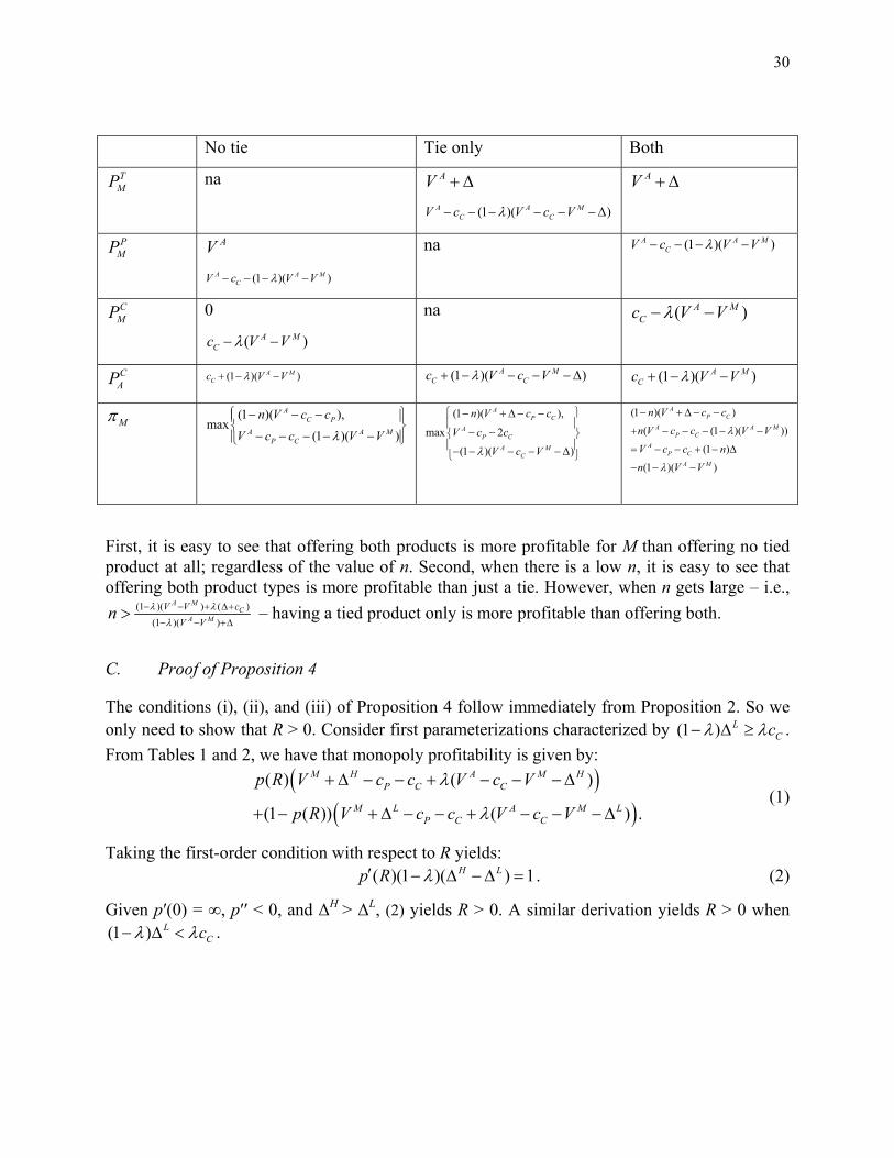
30

No tie Tie only Both T

MP na AV + Δ

(1 )( )A A MC CV c V c Vλ− − − − − −Δ

AV + Δ

PMP AV

(1 )( )A A MCV c V Vλ− − − −

na (1 )( )A A MCV c V Vλ− − − −

CMP 0

( )A MCc V Vλ− −

na ( )A MCc V Vλ− −

CAP (1 )( )A M

Cc V Vλ+ − − (1 )( )A MC Cc V c Vλ+ − − − −Δ (1 )( )A M

Cc V Vλ+ − −

Mπ (1 )( ),max

(1 )( )

AC P

A A MP C

n V c c

V c c V Vλ

⎧ ⎫− − −⎪ ⎪⎨ ⎬

− − − − −⎪ ⎪⎩ ⎭

(1 )( ),

max 2

(1 )( )

AP C

AP C

A MC

n V c c

V c c

V c Vλ

⎧ ⎫− + Δ − −⎪ ⎪

− −⎨ ⎬⎪ ⎪− − − − −Δ⎩ ⎭

(1 )( )

( (1 )( ))

(1 )

(1 )( )

AP C

A A MP C

AP C

A M

n V c c

n V c c V V

V c c n

n V V

λ

λ

− + Δ − −

+ − − − − −

= − − + − Δ

− − −

First, it is easy to see that offering both products is more profitable for M than offering no tied product at all; regardless of the value of n. Second, when there is a low n, it is easy to see that offering both product types is more profitable than just a tie. However, when n gets large – i.e.,

(1 )( ) ( )(1 )( )

A MC

A MV V c

V Vn λ λ

λ− − + Δ+

− − +Δ> – having a tied product only is more profitable than offering both.

C. Proof of Proposition 4

The conditions (i), (ii), and (iii) of Proposition 4 follow immediately from Proposition 2. So we only need to show that R > 0. Consider first parameterizations characterized by (1 ) L

Ccλ λ− Δ ≥ . From Tables 1 and 2, we have that monopoly profitability is given by:

( )

( )( ) ( )

(1 ( )) ( ) .

M H A M HP C C

M L A M LP C C

p R V c c V c V

p R V c c V c V

λ

λ

+ Δ − − + − − −Δ

+ − + Δ − − + − − −Δ (1)

Taking the first-order condition with respect to R yields: ( )(1 )( ) 1H Lp R λ′ − Δ −Δ = . (2)

Given p′(0) = ∞, p′′ < 0, and ΔH > ΔL, (2) yields R > 0. A similar derivation yields R > 0 when (1 ) L

Ccλ λ− Δ < .

31

REFERENCES

Adams, W.J. and J.L. Yellen, “Commodity Bundling and the Burden of Monopoly,” Quarterly Journal of Economics, 1976, 90, pp.475-498.

Bork, R.H., The Antitrust Paradox: A Policy at War with Itself, New York: Basic Books, 1978.

Bowman, W.S., “Tying Arrangements and the Leverage Problem,” Yale Law Review, 1957, 67, pp.19-36.

Carbajo, J., D. de Meza, and D.J. Seidman, “A Strategic Motivation for Commodity Bundling,” Journal of Industrial Economics, 1990, 38, pp.283-298.

Carlton, D.W. and M. Waldman, “The Strategic Use of Tying to Preserve and Create Market Power in Evolving Industries,” Rand Journal of Economics, 2002, 33, pp.194-220.

Carlton, D.W. and M. Waldman, “How Economics can Improve Antitrust Doctrine towards Tie-In Sales,” Competition Policy International, 2005, 1, pp.27-40.

Carlton, D.W. and M. Waldman, “Tying, Upgrades, and Switching Costs in Durable Goods Markets,” mimeo, Cornell University, 2006.

Chen, Y., “Equilibrium Product Bundling,” Journal of Business, 1997, 70, pp.85-103.

Choi, J.P. and C. Stefanadis, “Tying, Investment, and the Dynamic Leverage Theory,” Rand Journal of Economics, 2001, 32, pp.52-71.

Director, A. and E. Levi, “Law and the Future: Trade Regulation,” Northwestern University Law Review, 1956, 51, pp.281-296.

Evans, D. and M. Salinger, “Why do Firms Bundle and Tie? Evidence from Competitive Markets and Implications for Tying Law,” Yale Journal of Regulation, 2005, 22, pp.37-90.

Farrell, J. and M.L. Katz, “Innovation, Rent Extraction and Integration in Systems Markets,” Journal of Industrial Economics, 2000, 48, pp.413-432.

Gans, J.S., “Remedies for Tying in Computer Applications,” mimeo, Melbourne, 2007.

Miao, C., “Bundling, Compatibility and Upgrades,” mimeo, University of South Carolina, 2007.

Nalebuff, B., “Bundling as an Entry Barrier,” Quarterly Journal of Economics, 2004, 119, pp.159-187.

Nash, J.F., “The Bargaining Problem,” Econometrica, 1950, 18, pp.155-162.

Ordover, J.A., A.O. Sykes, and R.D. Willig, “Nonprice Anticompetitive Behavior by Dominant Firms Toward the Producers of Complementary Products,” In F.M. Fisher, ed., Antitrust and Regulation: Essays in Memory of John J. McGowan, Cambridge, MA: MIT Press, 1985.

Posner, R.A., Antitrust Law, An Economic Perspective, Chicago: Univ. of Chicago Press, 1976.

Whinston, M.D., “Tying, Foreclosure, and Exclusion,” American Economic Review, 1990, 80, pp.837-859.

32

Whinston, M.D., “Exclusivity and Tying in US v. Microsoft: What We Know and Don’t Know,” Journal of Economic Perspectives, 2001, 15, pp.63-80.