why is japan's saving rate so apparently high?piketty.pse.ens.fr/files/hayashi86.pdf ·...

This PDF is a selection from an out-of-print volume from the National Bureau of Economic Research

Volume Title: NBER Macroeconomics Annual 1986, Volume 1

Volume Author/Editor: Stanley Fischer, editor

Volume Publisher: MIT Press

Volume ISBN: 0-262-06105-8

Volume URL: http://www.nber.org/books/fisc86-1

Publication Date: 1986

Chapter Title: Why Is Japan's Saving Rate So Apparently High?

Chapter Author: Fumio Hayashi

Chapter URL: http://www.nber.org/chapters/c4247

Chapter pages in book: (p. 147 - 234)

Fumió HayashiOSAKA UNWERSITY, JAPAN

Why Is Japan's Saving RateSo Apparently High?

1. Introduction

The huge U.S. trade deficit with Japan, which totaled $50 billion in 1985and accounts for a thumping one-third of the total U.S. trade deficit, hasworried policy makers and economists alike for some time. The widen-ing trade gap has cost jobs in the United States, particularly in the manu-facturing sector, providing ample ammunition for protettionists. Theidentity in the national income accounts states that the excess of savingover investment equals the trade surplus. The blame for Japan's largetrade surplus with the United States must therefore fall on Japan's highsaving or her slumping investment. The widespread sentiment that theJapanese save too much was even echoed in a 1985 speech by the U.S.Secretary of State.1 The sentiment has some empirical grounds. In 1984the most widely mentioned saving rate—the rate of personal saving—was 16 percent for Japan, a full 10 percentage points higher than that inthe United States.

The purpose of this article is to explore possible factors that contributeto Japan's high saving rate. That Japan's saving rate is high by inter-national standards has been recognized in Japan for more than two de-cades, yet the reason for it is poorly understood: I quote the last sentenceof a recent survey in the Japanese literature. "In any event . . . Japan'shigh personal saving rate remains a mystery to be resolved."2 It is notthat empirical investigations have been hampered by a scarcity of data.Although consistent time series in the Japanese national income ac-counts do not start until 1965, a large amount of micro data on house-

1. George Shultz's speech at Princeton University attracted widespread attention in theJapanese press.

2. Kurosaka and Hamada (1984).

148 HAYASHI

holds is available from various surveys that have been conductedregularly by the Japanese government. Perhaps the issue of Japan's highsaving rate has not attracted enough of the empirical attention itdeserves.

I will begin with very down-to-earth facts about aggregate saving inJapan and the United States. Those are contained in section 2, whichtries to see if the perception of high savings in Japan has any empiricalbasis. It will be argued that some conceptual differences between U.S.and Japanese national accounting explain a substantial portion of the ol,-served differences in the saving rates. Section 3 summarizes the explana-tions that have been offered in the literature, (I will examine them furtherin later sections.) The first theory of saving, to be taken up in section 4, isthe life-cycle hypothesis. After rejecting the life-cycle explanations, Iturn in section 5 to micro data on households analyzed by age groupto locate possible deviations from the life-cycle hypothesis of the actualJapanese saving behavior. It turns out that the cross-section age profile ofsaving in Japan appears to defy any simple life-cycle explanation, includ-ing an explanation based on the high housing-related saving by youngergenerations. Continuing the theme at the end of section 5 that bequestsmight be an important factor, section 6 digresses somewhat to calculatethe aggregate flow of intergenerational transfers that can be inferredfrom the cross-section saving profiles. Other aspects of household be-havior, including the impact of social security, relevant to assessing theimportance of bequests will be analyzed in section 7. Section 8 thentakes up a separate issue, tax incentives for saving. The Japanese tax sys-tem does seem to be geared to promote saving. Taxes, however, are prob-ably not the main factor behind the high saving rate, I argue, becausesaving does not appear to be responsive to interest rates.

2. Facts about Japan's Aggregate Saving Rates2.1. WHICH SAVING RATE?

When comparing saving behavior between the two countries, we mustfirst decide which saving rate to use. The choice of the saving rate hasseveral dimensions. The first is the boundary of the relevant sector.Should we look at the household sector, the private sector, or the nationas a whole? The focus on personal (household) saving is unwarranted ifundistributed profits (corporate saving) are fully reflected in the capitalgains in stock prices that are recognized by households as part of in-come, or if corporations are just an accounting device for individuals to

Japan's Saving Rate 149

receive corporate tax treatment on their income.3 We should then look atprivate saving (the sum of personal and corporate saving). But even pri-vate saving is inappropriate if the private sector can see through the gov-ernment veil and internalize the government budget constraint. TheRicardian Equivalence Thorem states that a government budget deficit isrecognized by the private sector as a tax of the same amount because thepublic debt is just a signal of future increased taxes. The relevant notionof saving then is national saving (the sum of private and government sav-ing). The question of the relevant boundary is one of the basic issues ineconomics yet to be resolved, and in this article we will not commit our-selves to any one particular saving rate. We should, however, bear inmind that the substance of the corporate sector in the Japanese NationalAccounts is somewhat different from corporate business in the U.S. National Income and Product Accounts. At one end of the corporate sectorin the Japanese national accounts there are numerous token corporationsthat are essentially a disguised form of the household sector. At theother end lie most government enterprises (induding the central bank aswell as institutions that are not corporations in the legal sense).'

The second dimension in the choice of the saving rate is the definitionof income. Should we indude in income, and hence in saving, revalua-tion (capital gains/losses) of assets? Perhaps fully anticipated revaluationshould be included, but that is difficult to identify. If revaluation is recog-nized as part of income, private saving is a more meaningful saving con-cept than personal saving.

The third dimension is the scope of assets, which is where the treat-ment of consumer durables is relevant. In principle, any commodity thatis durable should be regarded as an object of saving. But measurement ofthe durability of commodities in general is a difficult task.5 The impor-

3. The top combined national and local personal tax rate is currently 88 percent in Japan.(However, we are told, there is a footnote in the personal tax code that reduces the topmarginal rate to 75 percent.) People in high-income tax brackets can spread their in-come over their spouses and relatives by setting up a token corporation. By paying themhigh wages and by taking advantage of the more generous tax deductibility provisionsin the corporate tax codes, they can understate corporate income and thus avoid doubletaxation at the corporate and personal levels. In 1983 there were about 1.8 million corpo-rations in Japan. The largest 1.2 percent paid close to 70 percent of the total corporationtax. About 60 percent of all corporations reported negative taxable income.

4. The Japanese national accounts also divide the nation into private and public sectors.Government enterprises are included in the public sector. In retrospect, the focus onprivate sector might have been more appropriate. Fortunately, as we shall see later, thedifference between the national and the private saving rates is small compared to thedifference of the personal rate from the private and the national saving rates.

5. A good example is dental services, it is classified as services in the national accounts but

w

150 HAYASHI

tance of consumer durables will be touched upon when we compare thepersonal saving rate between the two countries in figure 2. Dependingon the stand one takes in each of the three dimensions, there can be mul-titudes of saving rates. Only a subset of the possible saving rates will bediscussed in the text. The data appendix to this paper provides informa-Hon necessary for calculating not only the saving rates discussed in thetext but also several others that the reader might care to entertain.

2.2. DATA COMPARABILiTY

Even after the choice of the saving rate is made, there is a measurementproblem that makes international comparison tricky. There are (at least)four major conceptual differences between the United States and Japanin the compilation of national accounts.

1. A very surprising fact about the Japanese national income accountsis that depreciation is valued at historical costs.6 This means that personalsaving is overstated during and after the inflationary period of the1970s.7 Remember that personal disposable income is a net concept—itexdudes depreciation of household assets. Since personal saving is de-fined as personal disposable income minus consumption, it is net of de-preciation. Corporate saving is severely overstated for the same reason.There must, however, be an official estimate of replacement-cost de-preciation floating around within the Economic Planning Agency, thestatistical miU of the Japanese national accounts data, since the stock ofassets is valued at replacement costs in the capital accounts (balancesheets and stock-flow reconciliations) of the Japanese national accounts.Although the official estimate is neither published nor released, we canrecover it fairly accurately from the numbers published in the Annual Re-ports on National Accounts. Detailed descriptions of our calculation proce-dure and our estimate of capital consumption adjustments (the excess ofdepreciation at replacement costs over depreciation at historical costs)are given in the data appendix. The basic idea is to separate out the re-valuation component from the reconciliation accounts and identify theresidual as capital consumption adjustments. The calculation can bedone only for the post-1969 period because the capital accounts start in1970. Since investment goods prices were more or less stable until the

in essence it is a purchase of a durable good of good teeth. Hayashi (1985a) reports usingJapanese data that food is almost the only commodity that exhibits no durability. Recre-ational expenditures are found to be more durable than consumer durables.

6. Inventory valuation adjustments are incorporated in the Japanese national accounting.7. Investment goods prices more than doubled in the 1970s.


first oil crisis of 1973—74, the capital consumption adjustment is not sig-nificant for that period. However, the size of the adjustment to privatedepreciable assets has increased rapidly since then, reaching as muchas 30 percent of reported private saving in several recent years. (Seetable A2.)

2. Unlike most other countries (including Japan), the U.S. National In-come and Product Accounts compiled by the Bureau of Economic Analy-sis (BEA) treat all types of government expenditure as consumption andfail to credit the government for the value of its tangible assets. The BEAdefinition of government saving is therefore the government's budgetsurplus, while government saving in the Japanese national accounts in-cludes in addition the net increase in government tangible assets. Thisconceptual difference also means that even GNP and NNP are not di-rectly comparable because the BEA definition does not include outputservice flows from government tangible assets.

To make matters even more complicated, the Japanese national ac-counts do not depreciate government depreciable assets except buildings.Thus reported depreciation of government assets is very substantiallyunderstated: it is valued at historical costs and it covers only buildings. Inthe data appendix we constructed time series on the stock of governmentdepreciable assets by the perpetual inventory method and the associateddepreciation at replacement costs, so that the saving rate series for whichgovernment assets are included as components of assets can be con-structed for Japan. We decided not to construct such saving rate seriesfor the United States. When we compare the Japanese to the U.S. data, wewill recalculate the Japanese saving rates according to the BEA convention.

Readily available data sources on U.S. government capital accounts areRuggles and Ruggles (1982) and Eisner (1985).8 The definition of govern-ment assets in Ruggles and Ruggles appears comparable to that in theJapanese national accounts, but the data do not extend beyond 1980. Theratio to NNP of net government capital formation for the United Stateswas roughly around 1 percent in the 1970s. Eisner's data encompass amuch broader spectrum of assets and are thus not directly comparable.According to our estimate of government assets, the ratio to NNP of netgovernment capital formation is about 3—5 percent (see table A5). Thusthe exdusion of government capital alone makes a 2—4 percent differ-ence to the BEA definition of the national saving rate. However, it is notdear that all government capital formation should be counted as saving.Government investment projects in Japan, often politically motivated

8. The estimates of government capital in Boskin, Robinson, and Roberts (1985) are for thefederal government only.

-w

152 HAYASHI

and not necessarily justifiable on economic grounds, may be viewed bythe private sector as wasteful and incapable of yielding any useful ser-vice flows. It could even be argued that government capital is inherentlyunobservable, in which case it would be difficult to estimate the useful(as viewed by the private sector) asset lives for municipal buildings,highways, dams, and tunnels.

3. The Japanese national accounts do not adjust after-tax income for"capital transfers" (wealth taxes and lump-sum transfers), so in the capi-tal transactions (saving/investment) accounts the sum of saving, de-preciation, and capital transfers equals the sum of investment in tangibleand financial assets plus a statistical discrepancy. In what follows we in-dude transfers as part of saving, which is consistent with the U.S. prac-tice. For the household sector, capital transfers are negative because theyare mainly bequest and gift taxes. In 1984 these are about 5 percent ofreported personal saving. Almost all of the reduction of personal savingis transferred to corporate saving, making little difference to nationalsaving.

4. (very minor) In the U.S. national accounts personal consumptionand saving do not add up to personal disposable income because interestpaid by households to business and to foreigners is included in personaldisposable income. In what follows that interest component will be sub-tracted from U.S. personal disposable income.9

All the saving rates to be presented are adjusted as described above. Thedata source for Japan is the 1986 Annual Report on National Accounts(which incorporates the latest benchmark revision). For the U.S. NationalIncome and Product Accounts data we use the 1985 Economic Report of thePresident (which does not incorporate the January 1986 benchmark re-vision). It is supplemented by the Balance Sheets for the U.S. Economy,1945—84 (compiled by the Board of Governors of the Federal ReserveSystem) for balance sheet information, without addressing the questionof compatibility between the two sets of U.S. data.

2.3. A LOOK AT AGGREGATE SAVING RATES

The most widely cited evidence in support of the notion that the Japa-nese like to save far more than Americans do is Japan's exceptionally highpersonal saving rate (the ratio of personal saving to personal disposableincome). Is it still higher than the U.S. personal saving rate after theneeded adjustments? Figure 1 shows the adjusted personal saving ratefor Japan and the United States. Japan's personal saving rate in 1984 was

9. If the principal is reduced as a consumer repays loans, that reduction in principal is partof saving.


13.7 percent, about 2.5 percent lower than the personal saving rate re-ported in the national accounts and about 7 percent higher than the U.S.rate. The difference between the adjusted and the reported rate is mainlydue to the capital consumption adjustments. The adjusted personal sav-ing rate still exhibits the same basic pattern: it surges after the first oilcrisis of 1973—74 to a peak in 1976 of 21.1 percent. The U.S. personal sav-ing rate is stationary and has been fluctuating around 6 percent. It isclear that even after the needed adjustments Japan's personal saving rateis substantially higher.

Figure 2 shows the effect of including consumer durables as assets.Personal consumption thus excludes expenditures on durables but in-cludes gross service flows from consumer durables. Personal disposableincome now includes net service flows from consumer durables. A de-predation rate for consumer durables of 19 percent and a constant realrate of 4 percent are used for imputation. (See the data appendix for adetailed description of the imputation process.) It is well known in theUnited States that inclusion of consumer durables raises the personal sav-ing rate by a few percent. That is not the case for Japan—the personalsaving rate is little affected, thus narrowing the gap between the twocountries for 1984 to about 4 percent.

Figure 3 (and column (1) of table 1) displays the private saving rate (theratio of private saving to NNP, where Japan's NNP is calculated accordingto the BEA convention of not including net service flows from govern-ment assets). It does not include consumer durables. The U.S. rate ismore or less stationary. For Japan the behavior of the private saving rateis very different from that of the personal rate. It declines during and afterthe first oil crisis and has a declining trend since 1970. This is broughtabout by the sharp drop in corporate saving depicted in figure 4 whichshows the ratios of personal, corporate, and government saving to NNPfor Japan. (The NNP here includes service flows from government capi-taL) The corporate saving rate declined by 9 percent points from 1973 to1974 in the face of stagnant earnings, increased dividend payments, andincreased depreciation at replacement costs.

The BEA definition of the national saving rate, which excludes govern-ment net capital formation from national saving, is compared in figure 5for the two countries. It reveals a surprising fact about Japan—thoughone that is already apparent from a look at Japan's private saving rate infigure 3—that the national saving rate has declined quite sharply since1970. In the late 1970s there was only a small difference between the na-tional saving rates in the two countries. If one takes the view that private,not national, saving is the relevant saving concept, a good part of the de-

Tab

le 1

NE

T S

AV

ING

AS

PER

CE

NT

OF

NN

P W

ITH

AN

D W

ITH

OU

T R

EV

AL

UA

TIO

N

Japa

nU

nite

d St

ates

Yea

r(1

)(2

)(3

)(4

)(5

)(1

)(2

)(3

)(4

)(5

)

1970

23.8

25.6

2.1

—.4

51.2

7.8

—3.

1—

1.2

1.6

5.2

1971

20.8

28.7

2.0

—.9

50.6

8.6

.4—

2.0

1.3

8.3

1972

21.9

96.5

..1

—.3

118.

27.

77.

6—

.31.

316

.219

7321

.457

.81.

0—

1.0

79.2

9.2

9.4

.62.

421

.6•

1974

15.6

—89

.2.4

—1.

6—

74.7

7.6

4.1

— .4

3.4

14.7

1975

15.2

—13

.1—

3.5

—.4

—1.

8•

8.9

—.2

—4.

61.

85.

919

7617

.0—

8.8

—4.

7—

.23.

47.

77.

8—

2.4

1.6

14.8

1977

16.1

—.8

—4.

8.2

10.7

7.6

15.2

—1.

02.

123

.919

7818

.023

.5—

7.3

—.2

34.0

7.9

21.1

.02.

331

.319

7915

.552

.3—

5.4

.462

.87.

07.

3.7

2.8

17.8

1980

13.8

31.4

—4.

91.

742

.06.

11.

2—

1.3

3.0

8.9

1981

13.7

29.6

—5.

5.5

38.3

6.8

1.8

—1.

02.

19.

819

8212

.917

.4—

4.4

.526

.36.

1—

9.0

—4.

31.

5—

5.7

1983

12.4

1.9

—4.

9.5

9.9

6.7

—1.

0—

4.6

1.0

2.0

1984

12.5

2.0

—2.

6.6

12.4

8.4

—7.

5—

3.8

1.1

—1.

8

Ave

rage

16.7

17.0

—2.

8—

.030

.87.

63.

7—

1.7

1.9

11.5

(I)

Priv

ate

savi

ng.

(2)

Net

rev

alua

tion

(adj

uste

d fo

r ge

nera

l inf

latio

n) o

f pr

ivat

e ta

ngib

le a

nd f

inan

cial

ass

ets.

The

gen

eral

infl

atio

n ra

te d

urin

g th

e ye

ar is

rep

rese

nted

by

the

rate

of c

hang

eof

the

defl

ator

for

con

sum

ptio

n ex

pend

iture

fro

m th

e la

st q

uart

er o

l the

pre

viou

s ye

ar to

the

last

qua

rter

of

the

curr

ent y

ear.

(3)

Gov

ernm

ent b

udge

t sur

plus

.(4

) N

et r

eval

uatio

n of

gov

ernm

ent n

et f

inan

cial

ass

ets.

(5)

Sum

of

(1),

(2)

, (3)

. and

(4)

.

NN

P is

net

of

serv

ice

flow

s fr

om g

over

nmen

t tan

gibl

e as

sets

.

Dat

aA

ppen

dix.

I.

w — —

160 HAYASHI

dine in Japan's national saving rate after 1974 is attributable to the largebudget deficit shown in figure 4. Government saving, the sum of thebudget surplus and net government capital formation, has also beennegative since 1976, while reported government saving (not shown) hasbeen positive for all years.

The saving rates displayed thus far do not allow for revaluation or capi-tal gains/losses. This leads to an understatement of saving by net debtorsin an inflationary environment. Column (2) in table 1 reports net re-valuations—that is, changes in nominal values minus changes in valueattributable to changes in the general price level—on private (tangibleand financial) assets as a percent of NNP for Japan and the UnitedStates.'° (To make the Japanese data comparable to the U.S. data, I use theBEA convention here.) The huge capital gains and losses for Japan comeprincipally from the value of land, which is over 75 percent of the valueof total private assets. Column (3) in table 1 reports the size of the budgetsurplus (government saving under the BEA definition). Net revaluationof government net financial assets is in column (4). It shows the well-known fact that the U.S. government has gained substantially as a netdebtor. Since the ratio of net government financial liabilities to NNPwas low in Japan in the inflationary period of the 1970s (the ratio wasminus 6 percent in 1974) and since the inflation rate has been low in the1980s when the ratio is rapidly rising (it was 30 percent in 1984), net re-valuation for the Japanese government has been small. The total nationalsaving rate inclusive of revaluation is reported in column (5). The numberfor Japan may be overstated, as it is strongly dependent on the estimateof land value in the national accounts. The value of land in the privatesector (exduding government enterprises) at the end of 1984, accordingto the Japanese national accounts, is 858 trillion yen. It is substantiallyhigher than the market value of the U.S. private land of $3.3 trillion re-ported in the Federal Reserve's Balance Sheets.

2.4. MEASUREMENT OF DEPRECIATION

Coming back to the saving rates without revaluation, the impact of capi-tal consumption adjustments for Japan is most dramatically shown infigure 6 where the ratio of national saving to NNP (with government

70. The household and corporate sectors are already consolidated in table 1, because thedata on the market value of equity in the Japanese national accounts seem wholly unre-liable. The value of Tobin's q (the ratio of the value of tangible assets at replacement costto the market value of net financial liabilities) for the corporate sector at the end of 1984is 0.38 (see table A4). The reported market value of net financial liabilities is Less thanthe reported value of inventory. This low estimate is due to the fact that stocks that arenot publidy traded are valued in the Japanese national accounts at their" par" value (amere 50 yen). By consolidating the household and corporate balance sheets, the prob-

HAYASF{J

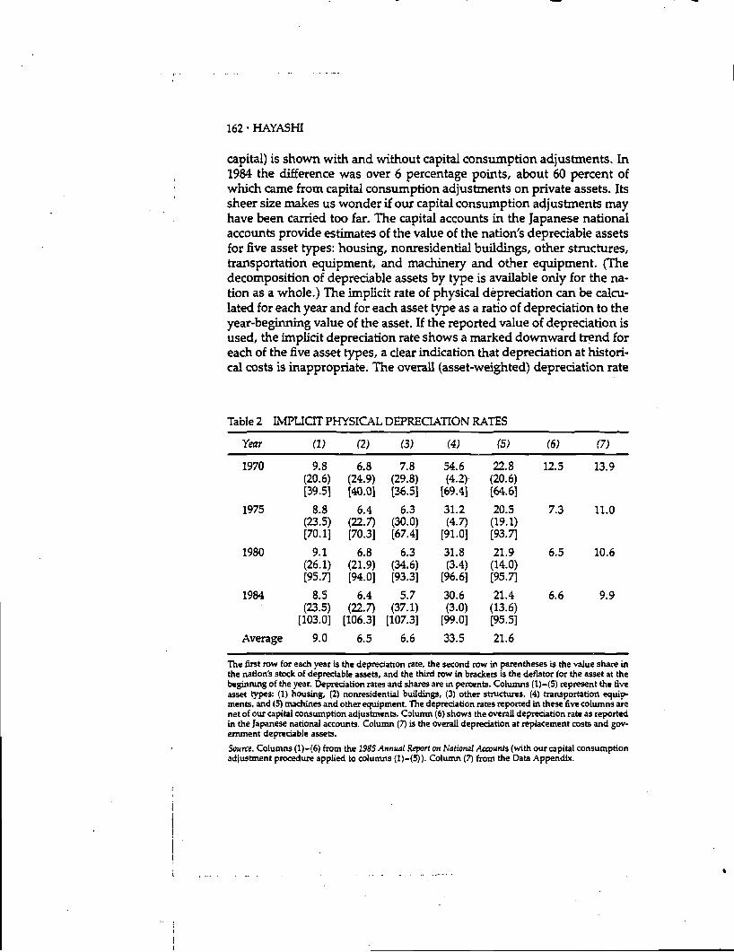
capital) is shown with and without capital consumption adjustments. In1984 the difference was over 6 percentage points, about 60 percent ofwhich came from capital consumption adjustments on private assets. Itssheer size makes us wonder if our capital consumption adjustments mayhave been carried too far. The capital accounts in the Japanese nationalaccounts provide estimates of the value of the nation's depreciable assetsfor five asset types: housing, nonresidential buildings, other structures,transportation equipment, and machinery and other equipment. (Thedecomposition of depreciable assets by type is available only for the na-tion as a whole.) The implicit rate of physical depreciation can be calcu-lated for each year and for each asset type as a ratio of depreciation to theyear-beginning value of the asset. If the reported value of depreciation isused, the implicit depreciation rate shows a marked downward trend foreach of the five asset types, a dear indication that depreciation at histori-cal costs is inappropriate. The overall (asset-weighted) depreciation rate

Table 2 IMPUCIT PHYSICAL DEPREUAflO('sI RATES

Year (1) (2) (3) (4) (5) (6) (7)

1970 9.8(20.6)(39.5]

6.8(24.9)140.01

7.8(29.8)(36.51

54.6(4.2)

[69.4]

22.8(20.6)(64.61

12.5 13.9

1975 8.8(23.5)(70.11

6.4(22.7)(70.31

6.3(30.0)(67.41

31.2(4.7)

[91.01

20.5(19.1)[93.7]

7.3 11.0

1980 9.1(26.1)[95.7]

6.8(21.9)[94.01

6.3(34.6)(93.31

31.8(3.4)

[96.61

21.9(14.0)[95.7]

6.5 10.6

1984 8.5 6.4 5.7 30.6 21.4 6.6 9.9• (23.5)

[103.01(22.7)

[106.31(37.1)

[107.31(3.0)

[99.0](13.6)[95.5]

Average 9.0 6.5 6.6 33.5 21.6

The first row for each year is the depreciation rate, the second row in parentheses is the value share inthe nation's stock of depreciable assets, and the third row in brackets is the deflator for the asset at thebeginning of the year. Depreciation rates and shares are in percents. Columns (1)—(5) represent the fiveasset types: (1) housing, (2) nonresidential buildings, (3) other structures, (4) transportation equip-ments, and (5) machines and other equipment. The depreciation rates reported in these five columns arenet of our capital consumption adjustments. Column (6) shows the overall depreciation rate as reportedin the Japanese national accounts. Column (7) is the overall depreciation at replacement costs and gov.ernment depreciable assets.

Source. Columns(1)—(6) from the 1985 Annual Report on National Accounts (with our capital consumptionadjustment procedure applied to columns (1)—(5)). Column (7) from the Data Appendix.


is reported for selected years in column (6) of table 2. It clearly shows theimpact of the 1973—74 inflation.

If our procedure for capital consumption adjustments, briefly de-scribed above, is applied to the five asset types to obtain depreciation atreplacement cost, we obtain the implicit depreciation rates reported in col-umns (1)—(5) of table 2 along with the asset shares in parentheses andasset price indexes in brackets. The depreciation rate for other structuresstill shows a downward trend, but it may be attributable to the practice

- in the Japanese national accounts of not depreciating government assetsother than buildings, which also distorts the asset shares in table 2in favor of structures. (The depreciation for transportation equipmentshows a steep downward trend for the first three or four years after 1970.We suspect that the 1970 value of the stock of transportation equipmentis understated.) The average depreciation rates in the last rows of col-umns (1)—(5) do not seem totally out of line with, for example, the aver-age implicit BEA rates reported in Hulten and Wykoff (1981, table 2)."Column (7) reports the overall depreciation rate implied by our capitalconsumption adjustment procedure and implicit in all the saving ratesdisplayed so far. It is not strictly the asset-weighted average of columns(1)—(5) because it is based on our estimate of government capital wherethe depreciation rate is constrained to be 6.5 percent. It still shows aclear but mild downward trend. This downward trend, which is notapparent in asset-specific depreciation rates in columns (1)—(5), is at-tributable to the shift in asset value shares in favor of longer-lived assets.This shift in turn is due mainly to the large-scale change in relative assetprices that has continued since at least 1970, shown in brackets. Itappears that our capital consumption adjustments are of reasonablemagnitude.

We conclude that Japan's aggregate saving rate—however defined—isindeed higher than the comparable U.S. saving rate, but not by as muchas is commonly thought. Not only is the level different, but the patternover time of Japan's saving rate with large peaks and well-defined trendsis in sharp contrast to the stationary U.S. pattern. We now turn to thequestion of how one might explain the difference.

lem of a correct valuation of equity can be avoided. This amounts to valuing corporatecapital at replacement cost rather than at the market value observed in the financialmarkets.

11. The average depreciation rates obtained in table 2 are close to the asset life reported inthe 2970 National Wealth Survey. Almost all the available estimates of the capital stock inJapan are based on this periodic official sampling survey of the net capital stock of thenation. The survey has not been conducted since 1970.

HAYASHI

3. A Catalogue of Explanations

That Japan's personal saving rate is one of the highest in the world wasrecognized in Japan as early as 1960. A concise survey of the early litera-ture can be found in Komiya (1966). The most recent and most exhaus-five survey is Horioka (1985b) which lists over thirty possible factors thatmight contribute to Japan's high personal saving rate. A striking featureof the Japanese literature is its lack of a neoclassical perspective: the per-sonal saving rate as a fraction of personal disposable income is the centerof attention. Also, no attention has been given to the measurement ofdepreciation which, as we have seen, is very important. This section isa catalogue of explanations of Japan's high saving rate that have beenoffered in the literature and still enjoy some currency. They will be exam-ined later.

High Income Growth An association of the income growth rate and thesaving rate is consistent with several alternative hypotheses of saving.Both the life-cycle hypothesis (with finite lives) and the permanent in-come hypothesis (with infinite horizon) imply that a temporary rise inthe growth rate raises the saving rate. For a permanent increase in thegrowth rate, the permanent income hypothesis would predict a lowersaving rate (if the real interest rate is unchanged). In the life-cycle hy-pothesis, the initial impact of a permanent increase in the growth rate onthe saving rate is probably to lower it, but the long-run impact is a highersaving rate, because older and dissaving generations are, in the long run,outweighed by younger and wealthier generations. The habit persistencehypothesis predicts a positive response of the saving rate to either a per-manent or a temporary increase in productivity growth. For Japan therelation between the growth rate and the saving rate is far from clear-cut.Figure 7 contains the graph of the GNP growth rate and the personalsaving rate. They tend to move in opposite directions, especially duringand shortly after the first oil crisis. This is inconsistent with the habitpersistence hypothesis. Comparing fIgure 7 with figures 3, 5, and 6, wesee that the private and the national saving rates are more dosely relatedto GNP growth than the personal rate.

The correlation of the saving rate with the growth rate is actually diffi-cult to interpret because there can be a reverse causation running fromsaving to growth through capital accumulation. However, the dear pre-diction by the life-cycle hypothesis that a secularly high growth rateshould be associated with a high saving rate could explain Japan's highersaving rate. This will be examined in the next section where we performa saving rate simulation based on the life-cycle hypothesis.

-4'—

Sav

ing

Rat

e0

Bon

us R

atio

-)'

GN

P

Figu

re 7

PE

RSO

NA

L S

AV

ING

RA

TE

, BO

NU

S R

AT

IO A

ND

GN

P G

RO

WT

H R

AT

E

Pers

onal

Sav

ing

Rat

e, B

onus

Rat

io a

nd G

NP

Gro

wth

Rat

e25 20 '5 l0

C ci) U ci)

0 -5-

65I

II

SS

II

I

6769

7173

7577

7981

83ye

ar

166' HAYASHI

Demographics The proportion of the aged has historically been small inJapan. Also, the life expectancy of the Japanese is now the longest in theworld. According to the life-cycle hypothesis, these demographic factorsshould raise the aggregate saving rate. This, too, will be taken up in thenext section.

Underdeveloped Social Security System The reasoning is that because Ja-pan's social security system is underdeveloped people have strong needsto provide for old by themselves. Japan's social security system hasexpanded rapidly since 1973. If the household sector is the relevantboundary, this explanation is inconsistent with the data because the per-sonal saving rate actually increased after 1973. The decline in the privatesaving rate could be explained by the eniarged social security system.The role of social security will be taken up in section 7.

Bonus System In postwar Japan, workers receive large lump-sum pay-ments twice a year. The bonus system originated in large firms and hasspread to smaller ones. The amount depends on the profitability of thefirm and the industry, although less so in recent years. The evidence thatappears to support this bonus hypothesis is that the ratio of bonuses toregular employee compensation is closely related to the personal savingrate, as shown in figure 7. (The data on the bonus ratio is from Ishikawaand Ueda (1984)). The bonus hypothesis was advanced very early andgained popularity when both the bonus ratio and the personal savingrate rose after 1973 and then slowly started to decline. This fact can,however, be explained straightforwardly by a neoclassical perspectivethat households can see through the corporate veil. Bonuses are a trans-fer of corporate saving to personal saving. If it is private saving thatmatters, the bonus ratio should raise personal saving. The bonus hy-pothesis cannot be an explanation of a high private saving rate.'2

Tax Incentives The Japanese tax system encourages saving because in-come from capital is very lightly taxed at the personal level. This issuewill be examined in section 8.

High Housing/Land Prices As Horioka (1985a) reports: 'The annual Pub-lic Opinion Survey on Saving.. . has consistently found that the fivemost important motives for household saving in Japan are those relatingto illness/unexpected disaster, education and marriage, old age, land/

12. Those who receive bonuses and those who own the company's stock are often differ-ent. The neoclassical reasoning is that they are linked with operative bequest and giftmotives.


housing purchases. and peace of mind. Moreover, a comparison of theJapanese findings and those of a similar U.S. survey shows that the big-gest differences are that the motives relating to education and marriageand land/housing purchases are far more important in Japan, while theold age motive is far more important in the United States." As docu-

in Hayashi, Ito and Slemrod (1985, incomplete), the Japanesehad to accumulate probably as much as 40 percent of the purchase priceof a house while borrowing the remaining fraction from governmentloans (subsidized and therefore rationed) and from private financial in-stitutions. The high ratio and the nondeductibility of in-terest expense for mortgage borrowing may contribute to high savingsby younger generations. Uke the first three explanations above, this ex-planation has life-cycle considerations in mind. Some evidence will bepresented in section 5 to gauge the relevance of high housing prices.

Bequests This is probably the least popular explanation in Japan. Thereis a casual discussion in Shinohara (1983) to the effect that perhaps theJapanese may like to leave large bequests. Horioka (1984), after rejectingthe standard life-cycle hypothesis on the basis of household survey dataand various opinion surveys, also notes at the end the importance of be-quests and their connection to the prevalence of the extended family inJapan. To anticipate, my conclusion is that bequests are probably themost important factor.

Cultural Factors If all else fails, there is a cultural explanation. The Japa-nese are simply different. They are more risk-averse and more patient. Ifthis is true, the long-run implication is that Japan will absorb all thewealth in the world. I refuse to comment on this explanation. Honoka(1985b), after examining various studies that address the cultural issue,concludes that the available evidence is mixed.

4. Explanation by the Life-cycle Hypothesis

The life-cycle hypothesis of saving (Modigliani and Brumberg (1954),Ando and Modigliani (1963)) asserts that, people's saving behavior isstrongly dependent on their age. Aggregate saving can be explained bysuch demographic factors as age distribution and life expectancy, andsuch economic factors as the age proffle of earnings. The hypothesis isattractive because it generates very specific empirical predictions- aboutaggregate saving if data are available on demographics, the age proffle ofearnings, and asset holdings. This section performs a standard "steady-state" simulation of aggregate saving under the life-cycle hypothesis.

168 HAYASHI

The steady-state assumption allows us to impute rather than observe theage profile of asset holdings. The profile of asset holdings by the age of a

- person (rather than by the age of a head of household) is difficult to ob-serve for the case of Japan because of the prevalence of the extendedfamily.

Before getting into the actual simulation, however, a precise defmitionof the life-cycle hypothesis is in order. Its essential feature, eloquentlyexpounded by Modigliaru (1980), is that people are selfish and do notplan to leave bequests. It is this feature which, coupled with the single-peaked age-earnings profile, leads to the prediction that people save toprepare for their retirement. An equally important, but often implicit,assumption is that people can purchase annuities and life insuranceat actuarially fair prices. This means (see Barro and Friedman (1977))there is only one constraint, the lifetime budget constraint, faced by theconsumer:

± r)1c(t + 1,1.' + i)

= + + i,v + i) + A(t,v), (1)

where c(t,v), -w(t,v) and A(t,v) are, respectively, consumption, earningsand initial assets of a consumer aged v at time i. q(t,v,i) is the probabilityat time t that the consumer of age v survives into period t + i. r is thereal rate of return. This version will be referred to as the strict life-cyclemodel.

In the absence of complete annuity markets, perfect insurance, as rep-resented by equation (1), against living "too long" is not available. Invol-untary bequests are the price to be paid to self-insure against longevityrisk. But, as Kotlikoff and Spivak (1981) point out, longevity risk canbe partially insured against if selfish parents "purchase," in exchangefor bequests, a promise by children to provide assistance in old age.This class of models may be called the selfish life-cycle model with im-perfect insurance.

Other models of saving include the strategic bequest model recentlyproposed by Burnheim, Shleifer, and Summers (1985) and the model ofdynastic altruism of Barro (1974) and Becker (1981). In the latter modelparents care about the welfare of their children and thus behave as iftheir planning horizon is infinite. In the former model, parents are notnecessarily altruistic toward their children but use bequests to influencetheir children's action. I do not here intend to confront all these modelswith the Japanese data in a formal fashion. Since most of the explana-

Japan's Saving Rate' 169

tions surveyed in the previous section have the strict life-cycle model inmind, the first order of business is to test it on Japanese data by a simula-tion technique.

If the strict life-cycle model is applicable to Japan, it should for realisticvalues of relevant parameter values generate the aggregate saving rateand the wealth-income ratio as observed in Japan. If we take seriouslythe numbers in the capital accounts of the Japanese national accounts,the ratio of national wealth (including, land) to (capital consumption-adjusted) NNP was about 4 in 1970 and about 6 in 1980 (see fIgure 8,where the inverse of the wealth-NNP ratio is plotted). The inputs to thesimulation are: (i) the actual age-earnings profile (w(t, v)), (ii) the actualage distribution of the population, (iii) survival probabilities (q), and (iv)a constant annual real rate of return of 4 percent. There are two param-eters: the longitudinal consumption growth rate (h) implicit in the age-consumption profile and the secular productivity growth rate (g). Thusthe longitudinal consumption profile is assumed to be

c(t + i,v + 1) = c(t,v)(l + h)1, (2)

and the prospective earnings profile is

w(t + i,v + i) = w(t,v)(1 + g)i. (3)

The potential lifespan is represented by seven ten-year periods. The firstperiod corresponds to ages 20—29 and the last to 80—89. Under thesteady-state assumption that earnings and assets of a consumer of givenage v grow at a constant rate g over time, we can calculate for each com-bination of h and g the aggregate saving rate and wealth-NNP ratio.'4

13. The age-earnings profile is constructed as follows. Earnings by age are taken from theBasic Survey of Wage Structure (the Ministry of Labor). They are multiplied by the laborforce participation rate taken from the Labor Ministry's Labor Force Survey. The earningsfor 50—59-year-olds are then multiplied by a factor of 1.18 to accommodate the re-tirement payments. This factor is calculated from the age-earnings profile displayedin Table 3-24 of the 1985 White Paper on Japanese Economy (Economic Planning Agency).The survival probability for a cohort in year t in a ten-year age group is calculated asthe ratio of the number of the cohort in year t + 10 to year t. For 1980, the survivalprobability is assumed to be the same as in 1970, except for cohorts over 60. Forthe 60—69-year-olds it is set at (1 — 0.01483)10, where the number 0.01483 is thedeath probability for 60—69-year-olds reported in a Ministry of Health and Welfarepublication. Similarly for the 70—79-year-olds the survival probability is set at (1 —o.046045)*lo.

14. Our "steady-state" simulation is a mere replication of the analysis in the second half ofTobin's (1967) paper but using Japanese data on the age-earnings profile and the agedistribution. To be more concrete, equations (1)—(3) are sufficient to give the prospectiveconsumption and asset holdings profile (c(t + i.v + i) and A(t + i,v ÷ i) for all i)

170 HA'YASHI

Table 3 displays the actual age profile, of earnings for 1970 and 1980with the sum normalized to unity, along with the U.S. earnings profile.15For lack of data, earnings for those aged 70 and over are set at zero. Theshare of earnings for ages 20—29 has declined in Japan, mainly due to adecline in the labor force participation rate brought about by the increasein college enrollment. Earnings in Japan peak in the 50—59 age group be-cause of lump-sum retirement payments. It may be argued that the highearnings by thos,e aged 50—59 do not reflect productivity; rather theearnings are a return from implicit saving whose amount equals the ex-cess of true productivity over actual earnings at younger ages. Withoutthe retirement payment adjustment, earnings for groups 40—49 and 50—59 are nearly the same, but the steady-state calculations do not change

for those aged v = 0 in period t because for v = Owe have A(t,O) 0 under the self-ish life-cycle hypothesis. The steady-state assumption implies that assets held byv-year-olds in period t + i are (1 ± g)**i times as large as assets held by v-year.olds in period t. That is, A(t + i,v) ((1 + g)**(_ i)) = A(t,v). This allows us tocalculate prospective consumption and asset holdings profile for those who are v yearsold in period t because their initial assets A(t,v) can be set at A(t + v,v) ((1 +g)**(_v)). The simulation is partial equilibrium in nature, because what is generated isthe supply of saving, that is not guaranteed to equal changes in the capital stock. Alsonote that the aggregate output growth rate depends on the age distribution as well ason the productivity growth rate g. Our simulation does not take taxes and transfersinto account. Proportional income taxes will not affect the saving and wealth-incomeratios. We also do not consider social security, because assumptions about future ex-pected benefits are inevitably arbitrary. If social security is actuarially fair, then it isdear that the size of the social security system does not affect our steady-state calcula-tions of the national saving rate.

15. The U.S. earnings profile is taken from the 1972—73 Consumer Expenditure Survey. Itwould have been preferable to obtain it from labor market data.

Table 3 AGE DISTRIBUTION OF EARNINGS AND POPULATION

Earnings

20—29 30—39 40—49 50—59 60—69 70—79 80—89

Japan, 1970Japan, 1980United States,

1972—73

0.120.09

0.17

0.22 0.28 0.13 0.00.22 0.28 0.29 0.13 0.0

0.24 0.26 0.22 0.11 0.0Population (Fraction of total population)

0.00.0

0.0

20—29 30—39 40—49 50—59 60—69 70—79 80—89

Japan, 1970Japan, 1980

0.190.14

0.16 0.11 0.09 0.06 0.030.17 0.14 0.11 0.07 0.04

0.010.01

See footnote 13 for the source of the Japanese data. The U.S. earnings profile is obtained from the Con-sumer Expenditure Survey, 1972—73, Bureau of Labor Statistics Bulletins 1992 and 1997. Table 3.

Saving rate (%)

Annual productivity growth

0% 5% 10%

3 —81 —68032 28 —8752 66 53

Saving rate (%)


0% 5% 10%

8 —64 —59633 27 5752 68 60

U.S. Earnings Profile, Japanese

Saving rate (%)


0% 5% 10%

7 —50 —40034 30 —4754 70 61

Saving rate (%)


0% 5% 10%.

10 —35 —33034 36 —2353 72 67

Wealth-income ratio


0% 5% 10%

—0.5 —7.8 —30.46.6 1.2 —4.1

10.0 5.0 1.9

Wealth-income ratio


0% 5% 10%

—0.9 —8.9 —35.17.0 1.5 —3.9

• 10.5 5.5 2.3

Age Distribution of Population

Wealth-income ratio


0% 5% 10%

1.1 —5.0 —17.97.5 2.2 —2.3

10.6 5.4 2.3

Wealth-income ratio


0% 5% 10%

1.6 —5.28.5 2.2 —1.9

11.6 6.1 2.8

In Panel B, the actual 1970 Japanese age distribution of population is used for 1970, and the actual 1980Japanese age distribution of population is used for 1980.


Table 4 STEADY-STATE SIMULATION RESULTS

Panel A. Japanese Earnings Profile, Japanese Age Distribution of Population

1970

Annualconsumptiongrowth (h)

h = 0%5%

10%

1980


h = 0%5%

10%

Panel B.

1970


h = 0%5%

10%

1980


h = 0%5%

10%

172 HAYASHI

significantly.'6 Table 3 also shows the actual age distribution of the popu-lation over the seven age groups. The postwar baby boom generation isnow approaching the prime earning ages. There are now more 40—59-year-olds, which should increase the aggregate saving rate.

The steady-state values of the aggregate saving rate and wealth-incomeratio expressed at annual rates are shown in table 4. The table suggestsseveral conclusions: Consumption must rise very rapidly through life forthe selfish life-cycle model to be consistent with the observed values ofthe aggregate saving and wealth-income ratios, because the Japaneseage-earnings profile is much steeper. To isolate the effect of the earningsprofile, Panel B of table 4 displays the simulation result which uses the1972—73 U.S. earnings profile for both the 1970 and 1980 simulations, butstill uses the same actual Japanese age distribution of population. Com-paring the saving rates in Panel B with those in Panel A for the same yearfor each combination of the consumption growth rate and the productiv-ity growth rate, we can see that with the age structure fixed the differ-ence in the earnings profile between the United States and Japan shouldmake the U.S. saving rate higher. Looking at Panel B for 1970 and 1980 andthus holding the age profile of earnings fixed, we see that the Japanesedemographics also work against the life-cyde hypothesis: it predicts arising aggregate Japanese saving rate.

Another surprising conclusion is that the saving rate generally declineswith the productivity growth rate under the Japanese age-earnings pro-file and demographics. This has a clear and simple explanation. Sinceearnings are highly skewed toward older ages, quite contrary to theusual textbook picture of hump saving, saving is done primarily by oldergenerations. As the secular productivity growth rate goes up, aggregatesaving becomes dominated by a younger and wealthier generation whosesaving rate is lower than the saving rate for older generations. It is stilltrue that the very old are dissaving, but their weight in the actual agedistribution is tiny.

Since a primary source of the failure of the life-cyde model to mimicthe observed saving and wealth-income ratios is dissaving by youngergenerations, the introduction of liquidity constraints may alter the con-dusion. The result (not shown) of a simulation in which consumption isconstrained not to exceed the sum of income and initial assets indicatesthat the saving and wealth-income ratios are now higher because thenegative saving by the young is constrained from below, but that the de-

16. This is because what is crucial in the simulation turns out to be the steepness of theJapanese age-earnings profile. See Hashixnoto and Raisian (1985) for a full documenta-tion on the effect of tenure on earnings in Japan and the United States.

Japan's Saving RateS 173

mographics still works dearly against the model and the inverse relationof the aggregate saving rate with the productivity growth rate remains.

5. Evidence from Household Survey Data5.1. HOUSEHOLD SURVEYS

The failure of the steady-state life-cycle simulation to mimic the aggre-gate saving rate and wealth-income ratio means that the actual Japaneseage profiles of consumption and asset holdings differ greatly from thelife-cycle predictions. We now examine them in order to locate possibledeviations of the Japanese saving behavior from the life-cyde models. Tothis end, survey data on households grouped by age of head of house-hold are essential. Several household surveys in tabulated form are pub-licly available in Japan. The Family Income and Expenditure Survey (FIES) isa monthly diary survey of about 8,000 households. It has no informationon assets and imputed rents and no information on income for house-holds other than the so-called worker household (namely, householdswhose head is on a payroll). The Family Saving annually collectsdata on balances and changes in financial assets and liabilities and pre-tax annual income. It has no information on expenditures and physicalassets. The sample size is less than six thousand, insufficient to give reli-able tabulations by age. These two surveys do not èover one-personhouseholds. The National Survey of Family Income and Expenditure (here-after National Survey), conducted every five years since 1959, is a verylarge sample (over 50,000) and covers most types of households (the ex-ceptions are agriculture and fishing). It obtains information through bi-weekly collection of diaries on expenditures on various items, imputedrent, income, taxes, and financial assets. The shortcoming of this surveyis that it covers only three months (September, October, and November)and that except for the pretax income for the twelve-month period end-ing in November no information is available on monthly income andtaxes for nonworker households, which are about 30 percent of thesample. The 1974 and 1979 tapes on individual households have beenextensively analyzed by Ando (1985). Our present study uses only thepublished tabulations in the National Survey Reports.

Table 5A displays some cross-section information for the United States,taken from the 1972—73 Consumer Expenditure Survey. Table 5B containssimilar information for Japan taken from the 1974 National Survey Report.One-person households are counted as a half household in thetion for Japan. Since average monthly income and taxes are not availablefor nonworker households, we show disposable income, ccmsumptionexpenditure and the saving rate separately for worker households. In-

Tab

le 5

A S

EL

EC

TE

D F

AM

ILY

CH

AR

AC

TE

RIS

TIC

S, I

NC

OM

E A

ND

EX

PEN

DIT

UR

E B

Y A

GE

OF

FAM

ILY

HE

AD

, U.S

.,19

72—

73

<24

25—

3435

—44

45—

5455

—64

65+

Impl

ied

aver

age

N1P

Aav

erag

e

Hou

seho

lds

in th

e un

iver

se(m

illio

ns)

6.3

14.2

12.0

13.0

11.5

14.3

71.3

(tot

al)

Fam

ily s

ize

1.8

3.2

4.3

3.5

2.3

1.7

2.9

Pers

ons

65 a

nd o

ver

.0.0

.0.1

.11.

3.3

Perc

ent h

omeo

wne

rs9

4068

7374

6659

•

Dis

posa

ble

inco

me

(tho

usan

ds)

$5.6

$9.9

$12.

2$1

3.3

$10.

6$6

.3$9

.9$1

2.4

Con

sum

ptio

n ex

pend

iture

(tho

usan

ds)

$6.5

$9.4

$11.

0$1

1.1

$8.5

$5.4

$8.8

$10.

9Sa

ving

rat

e (%

)—

155

1017

2013

128

Mar

ket v

alue

of

owne

dho

me

(tho

usan

ds)

$2.2

$11.

3$1

8.7

$19.

4$1

7.1

$12.

1$1

4.3

$11.

1

The

aver

ages

are

the

aver

ages

impl

ied

by th

e N

atio

nal I

ncom

e an

d Pr

oduc

t Acc

ount

s an

d th

e U

.S. B

alan

ce S

heet

s fo

r th

e to

tal n

umbe

r of

hou

seho

lds

of 7

1.3

mill

ion.

The

y ar

e av

erag

ed o

ver

1972

and

197

3.

Sour

ce:C

onsu

mer

Exp

endi

ture

Surv

ey.

1972

—73

. Bur

eau

of L

abor

Sta

tistic

s, B

ulle

tins

1992

and

199

7, T

able

S. 1

985

Eco

nom

ic R

epor

t vi t

hePr

esid

ent.

Bal

ance

She

ets

for

the

LI. S

.E

cono

my,

194

5—84

(Boa

rdof

Gov

erno

rs o

f th

e Fe

dera

l Res

erve

Sys

tem

).

Tab

le 5

B S

EL

EC

TE

D F

AM

ILY

CH

AR

AC

TE

RIS

TIC

S, I

NC

OM

E A

ND

EX

PEN

DIT

UR

E B

Y A

GE

OF

FAM

ILY

HE

AD

, JA

PAN

, 197

4

<24

25—

3435

—44

45—

5455

—64

65 +

Impl

ied

aver

age

NIP

Aav

erag

e

Hou

seho

lds

in th

e un

iver

se(m

illio

ns)

1.0

5.4

6.7

4.9

2.5

1.1

21.6

Fam

ily s

ize

2.2

3.5

4.3

3.9

3.6

3.5

(tot

al)

3.8

No.

of

olde

r pa

rent

s.0

6.1

7.2

5.2

7.3

2.2

7.2

4Pe

rcen

t hom

eow

ners

837

6275

8185

6019

74 p

reta

x in

com

e(m

illio

ns)

Y2.

1Y

2.2

Y2.

6Y

3.2

Y3.

1Y

2.5

Y2.

7Y

3.1

Con

sum

ptio

n ex

pend

iture

(mill

ions

)Y

1.6

Y2.

0Y

2.2

Y2.

0Y

1.7

Y2.

0N

et f

inan

cial

ass

ets

(mill

ions

)Y

.7Y

.9Y

1.3

Y2.

2Y

3.3

Y3.

6Y

1.7

Y3.

3M

arke

t val

ue o

f ow

ned

hom

e (m

illio

ns)

Y3.

1Y

3.6

Y3.

8Y

2.9

Y9.

8

For

wor

ker

hous

ehol

ds:

.

Dis

posa

ble

inco

me

(mill

ions

)Y

2.2

Y2.

3Y

2.5

Y3.

0Y

2.7

Y2.

2C

onsu

mpt

ion

expe

nditu

re(m

illio

ns)

YI.

6Y

1.8

Y2.

0Y

2.3

Y2.

1Y

2.0

Savi

ng r

ate

(%)

2521

2121

2121

21

As

the

Nat

iona

l Sur

vey

does

not

cov

er h

ouse

hold

sin

agric

ultu

re a

nd fi

shin

g, th

e nu

mbe

r of

hou

seho

lds

in th

e un

iver

se is

21.

6 m

illio

n (w

here

sin

gles

are

cou

nted

as

aha

il).

Itis

use

d to

cal

cula

te th

e N

IPA

ave

rage

s. T

he 1

974

pret

ax in

com

e is

(or

the

perio

d fr

om D

ecem

ber

1973

to N

ovem

ber

1974

. The

num

ber

of o

lder

pare

nts

livin

g w

ithth

e he

ad is

for

wor

ker

hous

ehol

ds.

Sour

ce:1

974

Nat

iww

l Sur

vey,

vol

. 1, p

art 1

, Tab

le 6

. 198

6 A

nnua

l Re,

url o

n N

atio

nal A

ccou

nts.

176 HAYASHI

come and expenditure variables are at annual rates.17 The value of àwnedhomes (which includes the value of land) is obtained from data on im-puted rent assuming that the annual real rate of return is 4 percent andthe depreciation rate 1 percent. The definition of disposable income andconsumption expenditure is brought closer to the national income defi-nition by using the following formulas:

consumption expenditure = total consumption expenditure+ income in kind (including imputed

rent), (4)

disposable income = total income (including social security benefitsand pensions)

+ income in kind (including imputed rent)* depreciation on owned home (20 percent of

imputed rent)— interest part of loan repayments (6 percent times

financial liabilities outstanding). (5)

Unless otherwise stated, this is the definition of disposable income andconsumption that we employ throughout the article. Although the re-maining conceptual differences make the comparison with the nationalaccounts data more or less meaningless (see Ando (1985) for detailed dis-cussion) it appears from the last two columns of table 5B that the Na-tional Survey severely underreports asset values.

From the viewpoint that the private sector or the nation is the relevant•boundary, the definition of income should include anticipated capitalgains on stocks. We should bear in mind that the saving rate displayed inthe tabulations is the personal saving rate, exclusive of revaluations. Weknow from table 1 that there were large capital losses on private assets in1974 and large capital gains in 1979. To the extent that some componentsof revaluation were anticipated, the saving rate for 1974 in table 5B isoverstated.

Several differences between the United States and Japan are dearly no-ticeable from tables 5A and 5B. First, the share in the total universe ofhouseholds headed by persons 65 and over is very small in Japan. Sec-ond, the average number of old people living with younger householdsis much higher. Third, home-ownership does not dedine after the house-

17. Monthly figures averaged over the three-month period of September through Novem-ber are converted to annual rates by using the seasonality factors reported in the An-nual Reports of the Family Income and Expenditure Survey.


hold head retires. These are just different aspects of the same importantfact about Japan, emphasized in Ando (1985), that elderly parents ofteninvite one of their children (usually the eldest son) and his family tomove into their house or, less frequently, the parents move into theyounger household. According to the Basic Surveys for Welfare Administra-tion, over 80 percent in 1960 and 67 percent in 1983 of persons 65 or overlived with their children. For persons 80 years or over, the proportionwas 90 percent in 1983. Thus data such as those given in table 5B orga-nized by age of head of household give only a mixture of the saving be-havior by the young and the old. This certainly makes the interpretationof the data less straightforward. We will come back to this issue of house-hold merging shortly.

5.2. HIGH HOUSING/LAND PRICES?

The fourth difference is that the saving rate does not depend very muchon age.18 This could be explained by the saving behavior of the elderlyliving with younger families, but, as we will see (in table 9, Panel A), thepattern is clearly observed for nuclear families as well. This is why thelife-cycle models fail to explain the Japanese saving rate. Fifth, unlikethe United States, there is no indication of dissaving by very younghouseholds. This can be explained by a combination of liquidity con-straints, the extremely high Japanese housing prices, and the high down-payment required to purchase a house.

This brings us to the explanation mentioned in section 3 that the Japa-nese saving rate is high because the Japanese have to save a great deal topurchase a house whose price is several times their annual income. TheNational Survey Reports since 1974 have separate tabulations for thethree largest metropolitan areas. We can therefore calculate the savingrate separately for urban and rural areas. Since housing prices are muchhigher in urban areas, the saving rate must be higher as well. We canactually get more information from the National Survey Reports becausesince 1979 the tabulations are further broken down to three householdtypes: homeowners; renters without a plan to purchase a house withinthe next five years; and renters with such a plan.

Table 6 displays the saving rate by region and household type for 1979and 1984. (As disposable income is not available for nonworker house-

18. This pattern shows up consistently in almost any household survey in Japan for everyyear. We must, however, be careful about the saving rate for the old. The saving rate isfor worker households, which automatically excludes But table 5B indicatesthat, for all households whose head is 65 or over, average annual income is 2.5 millionyen and average expenditure 1.7 million yen. For those households the average tax ratewould be at most 15 percent. Thus their personal saving rate must be over 20 percent.

178 HAYASHI

holds, the saving rate is calculated for worker households only.) As pre-dicted by the housing price hypothesis, the saving rate for renters withpurchase plans is several percent over that for other types of householdsin 1979. However, the saving rate for those who plan to purchase a housein urban areas is about the same as that in rural areas, which suggeststhat the elasticity of substitution between housing and other forms ofconsumption may be close to unity. It is not the price of houses per sethat is driving the saving rate up. More important are the unavailabil-ity of housing loans and the tendency of the Japanese to own, ratherthan rent, houses despite no tax advantages on mortgage payments.Another piece of evidence in the table unfavorable to the housing-pricehypothesis is that the saving rate averaged over household types is,if anything, higher for rural areas, where houses are much cheaper.This underscores the general principle that a high saving rate for theyoung population by itself does not translate into a high aggregate sav-ing rate. If for some reason or other the young are forced to save morethan they otherwise would, the life-cycle hypothesis implies that the in-voluntary saving will be spent in the later stages of life and thus reducethe saving rate for older generations. The high housing price does notseem to have any relevance in very recent years, because the table showsthat for 1984 saving rates are not at all affected by the intent to purchasea house.

5.3. ASSET HOLDINGS BY THE AGED

The prevalence of children living with parents creates two problemsthat must be borne in mind in analyzing Japanese household surveydata. First, as already mentioned, tabulation by age of the householdhead does not fully reveal the life cycle of a typical person, because of

Table 6 SAVING RATES BY AGE, TYPE AND REGION, WORKERHOUSEHOLDS

1979 1984

Urban Rural Urban Rural

1. Homeowners 18 19 18 202. Renters without

purchase plans 19 19 18 203. Renters with •

purchase plans 25 24 19 21

Average 19 19 18 20

Source: 1979 National Surt'ey Report. vol.Survey Report.

1, part I, Table 26, and vol. 1, part 2. Table 18. 1984 National


the presence of the elderly. in the extended family. Second, since thehousehold survey defines the head of a household to be the main in-come earner, there is a sample selection bias, in that heads of extendedfamilies in older age groups are high-income people whose earningsare greater than the earnings of their adult offspring in their prime earn-ing ages.

This sample selection bias is particularly relevant when we examinethe issue of asset decumulation by the aged, a popular test of the selfishlife-cyde models. Table 7 combines two of the tabulations given in Ando's(1985) study. The tableis arranged to make it easy to trace over the five-year period of 1974—79 the asset holdings by cohorts defined by five-yearage groups. The tabulation is for two-or-more-person households whosehead was over 56 in 1974, so both nuclear and extended families are in-cluded. Assets here consist of financial assets (excluding the presentvalue of social security benefits), the market value of any owned home(whose main component, of course, is the value of land), and consumerdurables. They are stated in 1979 prices. The mean asset holdings do notdecline as cohorts age. The essential aspect of the ]ife-cyde models doesnot seem to hold. This, however, is a premature conclusion, for threereasons. The first is probably familiar to American researchers, while theother two are specific to the prevalence of the extended family. First,

Table 7 AGE PROFILE OF ASSET HOLDINGS BY OLDER TWO-OR-MORE-PERSON HOUSEHOLDS, 1974 AND 1979

1974

Age of head in 1974

56—60 61—65 66—70 71—75

Sample size 1572 1418 927 553Mean 1946 1936 1815 1813First quantile 1185 1153 1095 1107Second quantile (median) 1760 1755 1662 1660Third quantile 2455 2456 2293 2323

1979

Age of head in 1979

61—65 66—70 71—75 76—80

Sample sizeMean

16231971

1187 6151839 1865

2451847

First quantile 1160 1038 1080 965Second quantile (median)Third quantile

17852512

1565 16362351 2398

15152291

In ten thousands of 1979 yen.

Source: Ando (1985).

1-IAYASHI

poor people at the lower end of the 1974 asset distribution are morelikely to die and thus disappear from the asset distribution for 1979. Sec-ond, of old nuclear families, poor ones may be more likely to disappearas they are merged into younger households. Third, by the very designof the survey, older household heads of extended families are the oneswho still dominate their sons in terms of income. This is the sample se-lection bias mentioned above.

For these reasons the lower end in the 1974 asset distributions be-comes tapered as time goes on. However, it should still be the case that ifthe old are decumulating, the upper ends of the asset distribution shiftto the left. For those who were 56—60 years old in 1974, there is no attri-tion in the first place because the sample sizes for 1974 and 1979 areabout the same. Thus simply comparing the mean is enough to concludethat there is no asset decumulation. For the 61—65-year-olds in 1974,there is a slight reduction in the sample size (from 1,418 to 1,187), andthe whole upper end seems to have shifted to the left between 1974 and1979. But the shift is very small—averaging across quartiles less than10 percent over five years. For the 66—70-year-olds the sample size de-clines by a third over the five-year period. If assets were neither accumu-lated nor decumulated, the 1979 second quantile should be somewherebetween the 1974 second and third quantiles. But in the table the 1979second quantile is actually less than the 1974 quantile, indicating that as-•set decumulation may have occurred. We get the same conclusion for the71—75-year-olds. Thus, there is some evidence of slight asset decumula-tion by the old. We hasten to add, however, that the conclusion is basedon the assumption of no attrition for the upper end of the asset distri-bution. Also, the sample size for the very old may not be large enough todeem the quantile estimates reliable.

5.4. IMPORTANCE OF BEQUESTS

Thus, the evidence on old persons maintaining independent households -

with or without their children is not very favorable to the selfish life-cycle models. Does the same condusion apply to the elderly living withyounger generations—the majority of the older population in Japan?Ando (1985) claims that there is strong evidence that they decumulateassets. He drew this conclusion from an equation explaining asset hold-ings for preretirement households. The equation shows a positive effecton household assets of the presence of the elderly in the household. Thisby itself is not surprising because when older parents retire they bringpreviously accumulated assets to younger households. What is signifi-cant is that the positive effect rapidly declines as the age of the older per-


son increases. However, it seems that Ando's conclusion is prematurebecause it ignores the role of bequests.

The saving behavior of the elderly living with younger generations canbe inferred from a comparison of the nuclear family with the extendedfamily. Table 8 displays the age profile of pretax income, expenditure,and financial asset holdings for 1979 and 1984. Because the tabulation inthe 1979 and 1984 National Survey Reports by family type (nuclear and ex-tended) do not show income in kind and imputed rent by age, consump-tion expenditure and income in the table are not adjusted for it. Themarket value of owned homes cannot be estimated, either. Taxes also arenot shown because the National Surveys have no data on taxes for non-worker households. The profiles for nuclear families are in Panel A, andthe proffles for extended families (households with adults of more thanone generation) are in Panel B. One-person households are counted ashalf a nuclear household.19 If entries in Panel A are subtracted from thecorresponding entries in Panel B, we obtain Panel C. It therefore con-tains the difference in income, expenditure, and assets brought about bythe presence of older parents. Consistent with Ando's conclusion, finan-cial assets attributable to the elderly start to decline as we move to theright across age groups in Panel C.2° This pattern of asset decumulation bythe elderly, however, is inconsistent with the low expenditure relativeto income shown in Panel C. Although table 8 shows pretax income,similar tabulations (not shown) based on disposable income for workerhouseholds indicate that the average tax rate is somewhere between13 percent and 17 percent depending on age and family type and issomewhat higher for nuclear Thus if the pretax income is multi-plied by 0.85 it serves as a lower bound for the difference in personaldisposable income (though not adjusted for income in kind). Compari-son of this estimate of disposable income and consumption expenditure

19. At the time of writing, the 1984 National Survey Report was not yet published, but Iwas given access to the 1984 tabulations in computer printout form. The tabulation for1984 in table 8 does not take single-person households into, account. It would makelittle difference to the results.

20. The difference in financial assets for the 20—29 age group in Panel C is small for thesample selection bias I have mentioned. Because the survey defines the householdhead to be the main income earner, older persons in a young extended family wherethe household head is the son tend to be low-income people, unable to earn more than20—29-year-olds do. Their contribution to household assets is therefore small. Becausetable 8 is a cross-sectional tabulation of assets, we must also be aware of the cohorteffect due to economic growth that asset holdings by v-year-olds in year t + i are(1 + g) i times as large as asset holdings by v-year-olds in year t, where g is the long-term growth rate. The cross-sectional decline in asset holdings reported in Panel C ofthe table is too steep to be accounted for by the growth factor, however.

Tab

le 8

AG

E P

RO

FIL

E O

F IN

CO

ME

, EX

PEN

DIT

UR

E, A

ND

ASS

ET

HO

LD

ING

S B

Y F

AM

ILY

TY

PE, A

LL

HO

USE

HO

LD

S,19

79 A

ND

198

4

1979

, Pan

el A

(nu

clea

r)20

—29

30—

3940

—49

50—

5960

+

Hou

seho

lds

in th

e un

iver

se (

mill

ions

)Fa

mily

siz

ePr

etax

inco

me

Con

sum

ptio

n ex

pend

iture

Net

fin

anci

al a

sset

s

1.7

3.0

3545

2614

2086

6.1

3.8

4278

2917

1247

5.3

3.9

5356

3515

3052

•

3.1

3.2

6243

3863

6512

1.1

2.5

4917

2865

8604

Pane

l B (

exte

nded

)

Hou

seho

lds

in th

e un

iver

seFa

mily

siz

ePr

etax

inco

me

Con

sum

ptio

n ex

pend

iture

Net

fin

anci

al a

sset

s

0.1

4.6

4792

3016

1851

1.3

5.4

5188

3314

3148

1.5

5.3

5999

3954

4753

0.8

4.5

6728

4005

7326

0.4

5.5

7179

3794

8860

Pane

l C (

Pane

l B —

Pan

elA

)

Fam

ily s

ize

Pret

ax in

com

eC

onsu

mpt

ion

expe

nditu

reN

et f

inan

cial

ass

ets

.

1.6

1247

401

765

1.6

911

397

1901

1.4

643

439

P01

1.4

485

142

814

2.9

2262 92

925

6

1984

, Pan

el A

(nu

clea

r)20

—29

30—

3940

—49

50—

5960

+

Hou

seho

lds

in th

e un

iver

se1.

36.

26.

04.

21.

5Fa

mily

siz

e2.

93.

83.

93.

12.

5Pr

etax

inco

me

.36

5045

5557

4064

4655

50C

onsu

mpt

ion

expe

nditu

re26

2529

5535

6538

4331

48N

et f

inan

cial

ass

ets

1088

829

1967

6177

1017

4

Pane

l B (

exte

nded

)

Hou

seho

lds

in th

e un

iver

se0.

11.

41.

91.

40.

6Fa

mily

siz

e4.

65.

4•

5.4

4.6

5.3

Pret

ax in

com

e48

4256

6264

5269

6069

15C

onsu

mpt

ion

expe

nditu

re32

4933

4838

8740

8534

47N

et f

inan

cial

ass

ets

1304

3224

4489

7124

7841

Pane

l C (

Pane

l B —

Pan

elA

)

Fam

ily s

aze

1.7

1.7

1.5

.1.5

2.8

Pret

ax in

com

e11

9111

0871

251

313

65C

onsu

mpt

ion

expe

nditu

re62

439

332

124

330

9N

et f

inan

cial

ass

ets

215

2395

2522

947

—23

34

Inco

me,

exp

endi

ture

and

ass

ets

in th

ousa

nds

of 1

984

yen.

Inco

me

and

expe

nditu

re a

re n

ot a

djus

ted

for

inco

me

in k

ind.

Pre

tax

inco

me

is fo

r th

e pe

riod

from

Dec

embe

rof

the

prev

ious

yea

r to

Nov

embe

r of

the

curr

ent y

ear.

Sou

rce:

197

9 N

atio

nal

Surv

ey R

epor

t, vo

l.1,

par

t 1, T

able

23.

198

4 N

atio

nalS

urve

y R

epor

t.

HAYASHI

in Panel C indicates that the elderly in younger extended households areaccumulating. Put differently, then, how is it that nuclear families are ac-cumulating assets so rapidly without the help of parents?

Our answer is that nuclear families do receive help from their par-ents—in the form of bequests. As we move to the right across age groupsin Panel C, both parents and children (heads of household) get older.More and more parents die as they get older. If parents in an extendedfamily leave bequests, the extended family turns into a nudear familywith additional assets. Furthermore, as the head of a nuclear family getsolder, more and more parents who maintain independent householdsdie and leave bequests, not to extended families, but to the nuclear fam-ily. In short, for middle-aged and older families, being an extended fam-ily is more like a signal of not yet having received bequests. The nextsection formalizes this argument to arrive at the flow of intergenerationaltransfers.

6. Calculation of Intergenerational Transfers

The sharp contrast between positive saving and dedining assets shownin Panel C suggests a substantial amount of intergenerational transfers.We digress in this section to evaluate the quantitative importance ofbequests. Since saving and asset holdings by age 1979 are given intable 8, we can calculate asset holdings by age in 1984 that would havebeen obtained through saving accumulated over the five-year period1979—84 in addition to the 1979 asset were it not for intergenerationaltransfers. (This calculation becomes rather complicated because withineach age group there are inflows and outflows of households betweenthe nuclear and extended families.) The difference between the actualand predicted 1984 asset holdings is then attributable to transfers. Ag-gregating transfers over age groups of recipients, we arrive at an esti-mate of the aggregate flow of transfers over the 1979—84 period. Clearly,this procedure captures only intergenerational rather than intragenerationaltransfers. It is the former that we are most interested in. And the cap-tured flow of transfers would include bequests as well as gifts inter vivos.

This simple idea cannot be implemented for the 1979—84 period,though. For one thing, table 8 presents data by ten-year age groups,whereas we need tabulations organized by five-year groups. Second, thetable gives no information on real assets. The value of owned homes isby far the most important household wealth in Japan. Fortunately, the1969 and 1974 National Survey Reports do give such needed information,


albeit only for worker The age profiles of disposable in-come, consumption expenditures, and the sum of financial assets andthe market value of owned homes are displayed in table 9 for 1969 and1974. As in table 7, the tabulation for the second year in table 9 is shiftedto the left by five years for tracking cohorts. For example, the saving ratefor a typical nuclear family whose head was 25 to 29 years old in 1969 is17 percent. Moving down vertically in the same column across panels,we see that five years later its saving rate is 21 percent. To eliminate thesample selection bias that parents (who are also the household heads) inolder extended families are rich while parents (who are not the house-hold heads) in younger extended families are relatively poor, extendedfamilies in the 55—59 group are put into the 25—29 group, the 60—64group into the 30—34 group, and the 65-and-over group into the 35—39group. This is why data for 1974 for cohorts in the 50—54 age group in1969 get lost and are not shown in table 9. This means that we cannotcalculate transfers goingto the households in the 1969 50—54 group.

A somewhat detailed description of the calculation of the flow of inter-generational transfers is as follows. Households are classified into threecategories:

(a) young nuclear, whose head was under 55 in 1969 (and under 60 in1974),

(b) young extended, whose younger generation was under 55 in 1969(and hence under 60 in 1974),

(c) old independent, whose head was 55 or over in 1969 (and 60 or overin 1974, or may have disappeared due to death or household mergingby 1974).

As one-person households are counted as a half of (a), all householdsexcept for single-parent households (whose number is small and whichare ignored in our calculation) fall into one of the three categories. House-holds in (a) and (b) are further classified by five-year age groups accord-ing to the age in 1969. Thus table 9 contains the income, consumptionand asset information for (a) and (b). Let W(i,j,t) and S(i,j,t) be the aver-age total wealth and saving (at 1974 prices) of households of type i

21. The tabulations by age and family type (nuclear and extended) in the 1969 and 1974National Survey Reports have no separate listing of imputed rent, although income inkind is listed. The tabulation by age alone does list imputed rent, which shows a moreor less stable proportion to food expenditure across age. This proportion is used toseparate out imputed rent from income in kind. Disposable income and consumptionexpenditure are then calculated by the formulas (4) and (5) in section 5.

Tab

le 9

AG

E P

RO

FIL

E O

F IN

CO

ME

, EX

PEN

DIT

UR

E, A

ND

ASS

ET

HO

LD

ING

S B

Y F

AM

ILY

TY

PE, W

OR

KE

R H

OU

SEH

OL

DS,

1969

AN

D 1

974

1969

, Pan

elA

(nu

ctea

r)

Age

zii

196

9

25-2

930

—34

35—

3940

—44

45—

4950

—54

Hou

seho

lds

in th

e un

iver

se1.

41.

61.

71.

40.

90.

7Fa

mily

siz

e2.

73.

43.

83.

93.

83.

6Pe

rcen

t hom

eow

ners

1529

4151

5663

Dis

posa

ble

inco

me

1765

1729

•19

1321

3323

0224

32C

onsu

mpt

ion

expe

nditu

re14

6014

6016

0617

8619

4520

39Sa

ving

rat

e (%

)17

1616

1616

16T

otal

ass

ets

1640

2574

3124

3805

4027

4894

Pane

l B (

exte

nded

)

Hou

seho

lds

in th

e un

iver

se0.

20.

30.

40.

40.

20.

1Fa

mily

siz

e4.

65.

15.

35.

35.

25.

1Pe

rcen

t hom

eow

ners

7976

7978

7880

Dis

posa

ble

inco

me

2033

2100

2158

2348

2570

2695

Con

sum

ptio

n ex

pend

iture

1791

1899

1867

.20

1622

7123

19Sa

ving

rat

e (%

)12

1013

1412

14T

otal

ass

ets

4921

4844

4866

5209

6073

5799

Pane

! C

(Pa

nel B

—P

ane!

A)

Fam

ily s

ize

1.9

1.7

1.5

1.5

1.4

.1.

4D

ispo

sabl

e in

com

e26

837

124

421

526

926

2C

onsu

mpt

ion

expe

nditu

re33

143

926

123

032

628

0Sa

ving

rat

e (%

)—

24—

18—

7—

7—

21—

7T

otal

ass

ets

3282

2270

1742

1404

2046

905

Age

in 1

969

1974

,P

ane!

A(n

ucle

ar)

25—

2930

—34

35—

3940

—44

45—

4950

—54

Hou

seho

lds

in th

e un

iver

se2.

22.

11.

81.

50.

9—

Fam

ily s

ize

Perc

ent h

omeo

wne

rs3.

6 333.

9 463.

9 563.

7 673.

3 70— —

Dis

posa

ble

inco

me

Con

sum

ptio

n ex

pend

iture

Savi

ng r

ate

(%)

Tot

al a

sset

s

2218

1746 21

2480

2393

1887 21

3048

2641

2064 22

3770

2916

2320 20

4732

2954

2291 22

5237

— — —.

Pane

l B (

exte

nded

)

Hou

seho

lds

in th

e un

iver

se0.

50.

50.

50.

40.

3—

.Fa

mily

siz

ePe

rcen

tho

meo

wne

rs5.

2 885.

5 895.

4 905.

1 914.

8 89— —

Dis

posa

ble

inco

me

Con

sum

ptio

n ex

pend

iture

Savi

ng r

ate

(%)

Tot

al a

sset

s

2854

2206 23

6473

2759

2260 18

6226

2888

2324 20

6528

3205

2554 20

6750

3209

2528 21

7018

— — — —

Pane

l C (

Pane

l B —

Pan

elA

)

Fam

ily s

ize

Dis

posa

ble

inco

me

Con

sum

ptio

n ex

pend

iture

Savi

ng r

ate

(%)

Tot

al a

sset

s

1.6

636

459 28

3993

1.6

366

373

—2

3178

1.5

248

260

—5

2757

1.4

289

234 19

2019

1.4

255

237 7

1782

— — — — —

Inco

me,

exp

endi

ture

and

ass

ets

inth

ousa

nds

of 1

974

yen.

The

num

ber

of h

ouse

hold

s in

nuH

ions

. Inc

ome

and

expe

nditu

re a

re a

djus

ted

for

inco

me

in k

ind

and

impu

ted

rent

.Tot

al a

sset

s ar

e th

e su

m o

f net

finan

cial

ass

ets

and

the

mar

ketv

alue

ofow

ned

hom

es. D

ata

for

the

50—

54 a

ge b

rack

etfo

r 19

74ar

eno

tgiv

en,b

ecau

se th

eyar

ead

ded

to th

e 25

—29

bra

cket

.

Sou

rce:

196

9N

atio

nal S

urve

y R

epor

t, vo

l. 1,

Tab

le 1

7. 1

974

Nat

iona

l Sur

vey

Rep

ort.

vol.

1, T

able

s 6

and

21.

188 HAYASHI

(i = a,b) in age group j (j = 1 for the 25—29 group, j = 2 for the 30—34,and so forth) in year t. Let N(i,j,t) be the number of such households. Ifp(i,k;j) is the fraction of households in the (i,j) cell in year t (= 1969)movinginto the (k,j + 1) cell in t + 1 (= 1974), we have, for each ageband j,

N(a,j + l,t + 1) = N(a,j,t)p(a,a;j) + N(b,j,t)p(b,a;j), (6)

where we assume that young households never disappear. We assumethat the flow of saving in real terms is constant over the five-year periodfor each type of household. If L(i,j,t) is the predicted wealth (stated

a typical household in the (i,f) cell in year t that can beaccounted for by accumulated saving on top of initial assets in year t, itcan be written

L(i,j,t) = 5.0 * S(i,j,t) + W(i,j,t). (7)

Thus the aggregate flow of intergenerational transfers is

TR = + 1,1974)W(a,j + 1,1974)

— ZN(a,j,1969)p(a,a;j)L(a,j,1969)

— 2N(b,j,1969)p(b,a;j)L(b,j,1969), (8)

where all the wealth variables W(a,j + 1,1974), L(a,j, 1969) and L(b,j, 1969)are stated in 1974 prices. The first sum is actual aggregate wealth held inyear t + 1 (= 1974) by all households of type (a). The second sum is thewealth accumulated through saving by households that stayed in (a), andthe third sum represents the wealth of households which moved from(b) to (a) during the 1969—74 period. Here S(b,j,t) and W(b,j,t) are thosethat are attributable to the younger generation in the extended family.Note that intergenerational transfers occur only from (c) to (a) or from(b) to (a).

22. In equation (7) it is not necessary to multiply S(i,j,t) or W(i,j,t) by (1 + r), where r isthe real rate of return, because S(i,j,t) already incorporates the return from assets as itis defined as disposable income less consumption. [1 S( i,j,t) were defined as after-taxlabor income less consumption, then the interest rate adjustment would have been nec-essary. During the early 1970s revaluation of assets was substantial (see table 1). In theactual calculation of L(i,j,t), we multiplied S(i,j,t) by a factor of 2.13. This factor trans-lates net saving to saving inclusive of net revaluation. To calculate this factor, we firstcalculate annual personal net saving and net revaluation at 1974 prices, and then takethe averages over the 1970—74 period. The factor is the ratio of the sum of average realnet saving (14.5 trillion in 1974 yen) and average real net revaluation (16.4 trillion) to theaverage real net saving.


Table 9 gives data on: N(i,j,t) (1 = a,b; t = 1969, 1974), S(a,j,1969)and W(a,j,t) (t = 1969, 1974) for each j. To estimate S(b,j,1969) andW(b,j,1969), we have to divide the saving and wealth of the extendedfamily between the younger generation and the older generation. We as-sume the elderly neither accumulate nor decumulate. Thus their savingis zero (so that S(b,j,1969) = S(a,j,1969) for all j). .For the 25—29 age groupW(b,j, 1969) equals W(a,j,1969), so that from Panel C for 1969 we see theasset holdings by the elderly in the 25—29 group to be 3,282 thousandyen (in 1974 prices). Assuming a productivity growth rate of 5 percent,asset holdings by the elderly in the 30—34 group are then this 3,282 thou-sand multiplied by (1 — .05)**5, which enablesus to calculate W(b,j,t)for this age group, and so forth. Finally, the values for S and Ware blownup to agree with the implied aggregate averages to account for the under-reporting noted in table 5B. Data on p(b,a;f) can be obtained from the 1969mortality table assuming that parents are thirty years older than theirchildren. (If there are two parents in the extended family, p(b,a,j) shouldbe the probability that both parents die within five years.) We are thusassuming that an extended family becomes a nuclear family only whenthe dependent elderly die. Using equation (6), p(a,a;j) can be calculatedfrom p(b,a;f). This completes the description of the calculation procedure.

There is one problem of head counting: the number of nuclear familiesin the 30—39 age group in 1974 is too large to be accounted for by thenumber of extended and nudear families in the 25—34 group in 1969.(We see from table 8 that the same phenomenon happened between 1979and 1984.) Without further information, it is impossible to resolve thequestion of where those extra nuclear families came from. We decided toignore this 1969 25—34 group in the summation in equation (8). We havealready discarded the 1969 50—54 age group. This leaves only three agegroups for 1969: 35—39, 40—44 and 45—49. Thus our aggregation cap-tures only a part of aggregate flow of transfers.

The result is that aggregate wealth held by worker nuclear householdsin 1974 in the 40—54 age group stood at 78.0 trillion yen.u Of that, theamount that was accumulated by saving by those households since 1969in addition to their 1969 wealth holdings was 70.0 trillion yen. The flow

23. From Panel A for 1974 in table 9 the stock of aggregate total assets for the 1974 40—54 age group (i.e., the 1969 35—49 group) is: 1.8 • 3.770 + 1.5 * 4.732 + 0.9 * 5.237= 18.6. 11 this is multiplied by a factor of 3.55, we arrive at 66 trillion yen. The factor of3.55 is to adjust for the underreporting already mentioned. If we compare this factorwith the information given in the last two columns of table 55, the factor seems a bittoo large. The factor one can calculate from table 5B for financial assets is 3.3/1.7 1.9and for houses it is 9.8/2.9 = 3.4. But table SB is for all households. If the similar cal-culation is done for worker households and the asset-weighted average over financialassets and houses is taken, one comes out with the factor of 3.55.

190• HAYASHI

of transfers was thus 8 trillion yen. If this is adjusted by the fraction ofworker households in the universe, we arrive at an annual flow of 11.5 tril-lion. Compared with the 1974 year-end aggregate private wealth of 598trillion, it looks small. Our calculation thus captures only a part of thetotal flow of intergenerational transfers. Moreover, looking at the tabu-lation for 1969 in table 9, we note from Panel C negative savings and not-so-rapidly declining total assets. Thus the year 1969 might have been apoor (though inevitable) choice. Our calculations also rely on the averagetotal asset holdings for the 25—29 age group in 1969. But that averagemay be unreliable, since the estimated number of households in that cellis small. Thus, our estimate should be taken as a very loose lower boundfor the true aggregate flow of intergenerational transfers.

7. Intergenerational Transfers

The evidence already presented points to the importance of intergenera-tional transfers. Their implication for the aggregate saving rate, however,depends critically on whether or not they are based on intergenerationalaltruism. Even if parents are not altruistic toward their children, theystill leave bequests if they die prematurely (accidental bequests); be-quests are used as payments to children for their service rendered to carefor older parents; or parents hold wealth in bequeathable form to influ-ence their children's action. In any of the three models the implicationsof the standard life-cycle model for the saving rate would still hold. Al-though it is difficult to draw a firm conclusion from the data at our dis-posal about the nature of bequests, the following pieces of evidenceseem largely consistent with intergenerational altruism.

Saving by Retirees Japan's social security system was greatly expanded in1973. It is now essentially a pay-as-you-go system. Quite likely, thislarge-scale transfer of resources from the young to the old engineered bythe government was not anticipated. The average annual old age benefitper person covered by the annuity benefit program for those employedin the private sector (Kosei Nenkin, the largest public annuity program)is 538 thousand yen in 1974 and 1,360 thousand in 1983, an increase inreal terms of 53 percent. The model of dynastic altruism predicts thatthis increase will be entirely saved by the old to offset the government-engineered transfer. It is supported by the fact observable from a com-parison of income and consumption in Panel C of table 9 with Panel C oftable 8 that the saving attributable to the elderly in extended families ap-pears to have increased in several recent years. This is inconsistent with


the selfish life-cycle models, which predict that the increase in annuitieswill be consumed.

Does this conclusion favorable to dynastic altruism also apply to olderpersons maintaining independent households? Since 1969 the NationalSurvey Reports have data on pretax annual income, consumption expen-diture, and assets of retired couples where the husband is 65 or over andthe wife is 60 or over. They are shown in table 10. The personal savingrate shows no tendency to increase, which appears inconsistent withdynastic altruism. But for older households revaluation of assets may bean important component of income. For 1974 and 1979, there is a greatdeal of uncertainty in estimating net revaluation (revaluation excludingchange in value attributable to general inflation) that might have beenperceived by the households over the three-month period of Septemberthrough November, because as reported in the table (and also in table 2)price changes were so large. The real price of housing was more or less

Table 10 SAVING BEHAVIOR OF RETIRED OLDER COUPLES

1969 1974 1979 1984

Sample size 242 407 653 951Percent homeowners 80 81 81 86Percent of pension

recipients n.a. n.a. n.a. 94Pretax income 1494 1907 2278 2457Consumption expenditureIncome in kind

1082 1468 1872 1899

(mci. imputed rent) 285 302 n.a. n.a.Value of owned home 4581 5059 n.a. n.a.Net financial assets 4934 5566 6934 8684General inflation rate (%) 5.1 22.9 4.7 2.4Rate of change of deflator

for the stock of houses n.a. 7.7 13.7 2.2Rate of change of deflator

for housing investment 4.1 19.8 12.8 2.3Saving rate (%) 28 23 18 23Saving rate with . .

revaluation 13 ? ? 16

Income, expenditure and assets in thousands of 1984 yen. Income and expenditure are not adjusted forincome in kind. Pension recipients are defined as couples whose main souice of income is a public orprivate pension. The saving rate does not take taxes into account. The saving rate with revaluation in-cludes in income net revaluation of net financial assets. It is not calculated for 1974 and 1979 because ofthe uncertainty about the size of net revaluation of owned homes.

Source: 1969 National Survey Report. vol. 1, Table 24. 1974 National Survey Report, vol. 1, Table 27. 1979National Survey Report, vol. 7, Table 16. 1984 National Survey Report. 1986 Report on National Accounts.

192 HAYASHI

constant in 1969 and 1984, so that net an owned home canbe ignored. If only the net revaluation of financial assets is taken intoaccount, the saving rate is 13 percent in 1969 and 16 percent in 1984. Still,the sharp increase in saving predicted by dynastic altruism is absent.

It may be that, as conjectured in Ando (1985), the saving behavior ofolder persons who maintain independent households is different fromthat of older persons living with their children. This is perhaps not sur-prising. It is hard to imagine that social security has any big impact onthe consumption behavior of the elderly in the extended family, becausethere must be some in-house sense of proportion regarding consump-tion within the extended family. If social security benefits for older par-ents are raised with a simultaneous increase in the social security tax ontheir children living under the same roof, older parents, even without astrong sense of altruism toward their children, would find it morallyhard to raise their spending at their children's expense.

Euler Equation There is another way to examine the impact of social se-curity on the consumption behavior by the aged. Every five years since1959 the National Survey Reports have tabulations by age where the agegroups are also five years. Aswe did in table 9, we can track from year tto t + 1 a cohort in the jth 5-year age group in year t by looking at the(j + 1)th age group in year t + 1. For example, a cohort in the 20—24age group in 1969 was in the 25—29 age group in 1974. If C(j,t) and Y(j,t)are consumption arid disposable income of a representative cohort inage group j in year t, we can get from the National Survey Reports data onC(j,t) and Y(j,t) for j = 1 (20—24-year-olds), 2 (25—29-year-olds), . . .

9 (60—64-year-olds) (nine age groups) and for t = 1959, . . . , 1984 (sixtime points). Thus the synthetic cohort analysis as done by Browning,Deaton and Irish (1985) is feasible here. For each cohort, we assume thatthe Euler equation applies:

€nC(j + 1, t + 1) — enC(j,t) = a + b + e(j,t). (9)

Here, the left-hand side is the growth rate of consumption from year tto t + 1. When interest rates are high, it pays to reduce consumptionnow relative to future consumption. Thus the consumption growth rateshould increase with the expected real rate This is the expectationas of year tof + + where is the nominal rate on a5-year bond and P is the price index. The sum of the first two terms onthe right-hand side, a + fir,, is the planned rate of consumption growth.But actual growth can differ from the planned rate, perhaps because theinterest rate forecast proved to be wrong, or because earnings change un-


expectedly over the period t through t + 1. The last term e(j,t) repre-sents those unexpected developments happening to cohort j. As the1973 expansion of Japan's social security system was an unexpected de-velopment that transferred resources from younger generations to oldergenerations, the selfish life-cycle hypothesis predicts that consumptiongrowth from year 1969 to 1974 for older cohorts should be greater thana + and their e(j,t) positive.

As we have data on C(j,t) for six time points (1959, 1964, 1969, 1974,1979, and 1984), the consumption growth rate can be calculated for fiveconsecutive periods. Thus the sample size for estimating equation (9) is45 (five times nine age groups). Growth rates and interest rates are statedat annual rates. Because the Euler equation presupposes that expen-diture is perishable, we use food expenditure for consumption. Table 11reports various regression results. In all regressions, AGE (1 for 20—24-year-olds, 2 for 25—29-year-olds, and so forth) and AGE squared areincluded to account for possible age differences in the intercept term a inequation (9). Equation (9) is estimated in Regression 1. The actual realrate is used in place of It picked a wrong In Regression 2, to

Table 11 ESTIMATION OF EULER EQUATION ON SYNTHETICCOHORT DATA

Regression#

Realrate ofinterest

Socialsecuritydummy

Log of realdisposable

income R2

Otherincludedvariables

1 —0.14(1.8)

— — 0.55 AGE, AGE2.

2 —0.29(3.0)

—0.024(2.4)

— 0.61 AGE, AGE2

3 —0.027(0.5)

— —0.043(6.8)

0.79 AGE, AGE2

4 —0.098(1.3)

—0.011(1.4)

—0.041(6.2)

0.80 AGE, AGE2

5 — —0.013(1.9)

— 0.84 AGE, AGE2,time dummies

6 — — —0.13(4.9)

0.89 AGE, AGE2,time dummies

7 . — —0.010(1.8)

—0.12(4.7)

0.90 AGE, AGE2,time dummies

AU variables are stated at annual rates. The dependent variable is the growth rate of real food expen.diture over five-year periods. Real disposable income is the ratio of nominal disposable income to thefood component of the CPI. The nominal rate used to construct the real rate is the rate on 5-year dis.count bonds issued by financial institutions. The price index used to calculate the real interest rate is thefood component of the Cl'!. See the text for the definition of the social security dummy. Numbers inparentheses are the t values. The data source is the National Survey Reports.

194 HAYASHI

examine the impact of the unexpected 1973 expansion of the social secu-rity system, a dummy variable which takes a value of unity for cohortsover 44 years of age for the 1969—74 period is added to the equation.It also has a negative coefficient, which means, contrary to the life-cycle prediction, that the 1973 change reduced consumption by oldergenerations.

In regressions 3 and 4, the log of disposable income, €nY(j,t), is in-cluded to test for liquidity constraints with or without the social securitydummy. If people wish to borrow to finance current consumption butare prevented from doing so, a higher level of disposable income leads toan increase in current consumption, thereby reducing the consumptiongrowth over the following five years. Thus if there are liquidity con-straints, the disposable income variable should pick up a negative coeffi-cient, which is what is happening in regressions 3 and 4. The socialsecurity dummy still picks up negative coefficients.

For the expected real rate r1, we have used the actual real rate. Thisamounts to conferring on consumers perfect foresight about futureprices and thus may be unrealistic. Regressions 5—7 use time dummiesin place of the actual real rate. Thus the a + br, term in equation (9) canchange its value over the five periods, reflecting changes in the expectedreal rate and possibly economywide shocks that affect all generationsuniformly. Again, the disposable income coefficients are significantlynegative and the social security dummy picks up the "wrong" sign.

The Extended Family and Bequests Finally, the fact that most older parentsinvite their children to move in has two further implications for theoriesof bequests. First, because if older parents get sick or incapacitated chil-dren would feel obliged to take care of them, accidental bequests areclearly less important. Second, the merging of older and younger house-holds means that long before older parents' death there is a de factotransfer from older parents to the children of housing—by far the mostimportant component of wealth.24 The strategic aspect of bequests looksless significant for Japan.

24. The actual transfer of ownership does not usually occur until the death of the parents.In 1983 taxable bequests were valued at 5.0 trillion yen, while taxable gifts were 0.6 tril-lion (see Annual Statistical Report of the Tax Bureau, the only official source of data ontaxes in Japan). A standard guidebook on Japanese bequest and gift taxes indicates thatbequests are taxed slightly less heavily. The effective bequests tax rate is much lower onhouses than on financial assets, because the assessed value of real estate is often lessthan half the market value. This may explain why the Japanese prefer owning a houseto renting.


8. The Role of Taxes

To examine the only remaining major issue, the effect of taxes on saving,we need to address two issues. One is the effective marginal tax rate onincome from saving, and the other is the so-called (after-tax) interestelasticity of saving. A good deal of work has been done on the first issue.A comprehensive official description of Japan's tax system can be foundin An Outline of Japanese Taxes (various years) by the Ministry of Finance.A good economist's description is in Horioka (1985b, section 4), Shovenand Tachibanaki (1985) and Makin (1985). The treatment of personalinterest and dividend income in the Japanese tax system differs consider-ably from that in the United States. The notorious Maruyu system im-plies that interest income from a principal of up to 6 million yen (about$30 thousand) for "nonsalaried" workers and 12 million yen for "sala-ried" workers is nontaxable. Because abuse of this system is so common,it is difficult to estimate the marginal tax rate on interest income. Capitalgains on stocks are not taxed if the gain is less than a certain amount andif the number of transactions is not large (less than fifty transactions ayear). But this provision, too, can be avoided by trading stocks throughseveral different brokers. The tax rate on dividend income is at most 35percent, as high-income taxpayers can elect to have interest and dividendstaxed separately at that rate, and for many middle- and low-income earn-ers it is substantially less. Since the return from Japanese stocks has beenmainly in the form of capital gains, the average tax rate on income fromequity capital is very low. These facts led Shoven and Tachibanaki (1985)to assume very low marginal personal tax rates on interest income andincome from equity (9.6 percent and 18.1 percent respectively). The verygenerous tax treatment of income from capital at the personal level is insharp contrast to taxes on labor income whose top combined nationaland local statutory marginal rate is close to 80 percent.

At the corporate level, it appears that income is more heavily taxed inJapan than in the United Although there is not much differencein the statutory corporate tax rate, the U.S. treatment of depreciation al-lowances and investment tax credits is more generous, at least in the1980s. So the marginal tax rate on income from new capital at the corpo-rate level in Japan is higher. The generous tax treatment at the personallevel coupled with a relatively heavy tax burden at the corporate levelmust at least in part be responsible for the recent capital outflow fromJapan to the United States.

25. See Ando and Auerbach (1985) for a comparison of the cost of capital in Japan and theUnited States.

196• HAYASHI

The present Japanese tax system is thus geared to encourage saving.The other issue is whether it has been effective in promoting saving. Theconventional approach to analyzing the response of saving to changes inthe after-tax rate of return to saving is the saving function, which relatesaggregate saving to the after-tax interest rate. Because of many seriousproblems, including the Lucas critique, the saving function approachseems to have been discredited by now. The modem approach that re-places it is the Euler equation approach, discussed in the previous sec-tion, which looks at the relation between consumption growth and thereal interest rate. If saving is elastic to the interest rate, it should show upas a positive relation of the real interest rate with the growth rate of con-sumption from one period to the next, because increased current savingmakes the level of current consumption relative to future consumptionlower. The evidence presented in table 11, however, shows no such relá-tion; in fact the sign of the real rate coefficient is the opposite of the theo-retical prediction. Saving does not seem sensitive to the interest rate.

To check the robustness of this conclusion, the same form of the Eulerequation (9) is estimated on monthly aggregate data on food expen-

Table 12 ESTIMATION OF EULER EQUATION ON MONTHLYAGGREGATE DATA

Equation#

Realrate ofinterest

Log of realdisposable

incomeEstimationtechnique

Durbin-Watsonstatistic

la 0.10(1.1)

— forwardfiltering

• —

lb 0.11(4.3)

— OLS 1.3

2a 0.08(0.96)

—0.003(1.3)

forwardfiltering

—

2b 0.12(4.5)

—0.014(3.6)

OLS 1.4

The dependent variable is the growth rate of real food expenditure from the month to the month oneyear ahead, namely, The nominal rate used for constructing the real rate is the rate onone-year time deposits. The food component of the CPI is used to calculate the real rate. The log of realdisposable income is where is disposable income of month t divided by the food component ofthe Cl'!. Because the consumption growth rate is over one-year periods while the sampling interval isamonth, the error term will be a mov:ing average of order 11. The forward filtering technique proposed inHayashi and Sims (1983) is used for equations Ia and 2a. Because the ex-post real rate is potentiallycorrelated with the error term, it is instrumented in equations Ia and by the current one-year nomi-nal rate, current and 12 lags of the monthly food inflation rate, and current and 12 lags of the tog ofmonthly disposable income. They explain about 39 percent of monthly variations in the real rate. Thedata period is from January 1963 through October 1985. Numbers in parentheses are the t values. Thedata on monthly food expenditure and disposable income for worker households are taken fromthe Annual Reports of the Family Income and Expenditure Survey.


diture. The Annual Reports of the Family Income and Expenditure Surveycontain data since 1963 on average monthly expenditure and disposableincome for worker households. For reasons explained in the previoussection, food expenditure is used for the estimation. (For details of theestimation see the nOte to table 12.) The real rate coefficient is now posi-tive (the right sign), but still insignificantly different from zero. Thenegative effect of disposable income suggests the presence of liquidityconstraints, but it too is insignificant. The wrong sign of the real rate co-efficient found in table 11 may be explainable by the correlation betweenthe ex-post real rate (used for the expected real rate) and the error termthat represents unexpected developments (over the five-year periods).On the other hand, the real rate coefficients in table 12, while correctedfor the correlation with the error term, suffer from the possible aggrega-tion bias. The Euler equation holds for each individual. Since each yearthe oldest generations are replaced by new younger generations, it is notnecessarily true that the Euler equation holds for aggregate consump-tion, On the whole, then, there is no strong for a high interestelasticity of saving or for the effectiveness of the tax incentives for saving.

9. Concluding Comments

If one subscribes to the dynastic view of Barro (1974) and Becker (1981),it seems that all the evidence presented in this article—the insensitivityof the aggregate saving rate to demographics, saving rates that are inde-pendent of age, the possibly significant flow of intergenerational trans-fers, the insignificance of the social security dummy, and certainly theprevalence of the extended family—are parsimoniously explainable, al-though we must hasten to add that no direct and formal test of the dy-nastic model against other theories of bequests was given in the article.2'A large flow of bequests by itself does not lead to high saving rates. Onecan easily construct a stationary economy with a zero saving rate inwhich assets are passed on from one generation to the next and in whicheach generation consumes all of its income. The existence of a significantflow of bequests does, however, imply that the infinite horizon assump-tion may be a good approximation. Add to this the fact that Japan had to

26. The existence of liquidity constraints is not inconsistent with the dynastic model. Sup-pose that people do not come to realize the linearity of the family until they reachmiddle Until then the only limits on their consumption are liquidity constraints.Their parents do think about the family. Because of liquidity constraints they can deter-mine their impatient son's consumption through transfers. Thus family consumption iseffectively controlled by the parents. Also, liquidity constraints do not necessarily in-validate the Ricardian doctrine of the equivalence of taxes and deficits. See Hayashi(1985b).

Figu

re 8

NN

P—W

EA

LT

H R

AT

IO A

ND

SA

VIN

G A

ND

IN

VE

STM

EN

T R

AT

ES

4-20

U a) 0-IS30 25

Nat

iona

l Wea

lth, S

avin

g an

d N

et In

vest

men

t

I0 0 70 7

1 72

73

74 7

5 76

77

78ye

ar79

80

81 8

2 83

84


start with a low level of wealth. The infinite horizon optimal growthmodel implies that the economy's response to the low initial wealth is ahigh saving rate that gradually stabilizes to a lower level as wealth ap-proaches its steady-state value. Japan's saving rate has been high becausethe Japanese desire to accumulate wealth in order for their children tolive as well as Americans do.

That this simplistic view is consistent with Japan's experience in thelast fifteen years (though not in the 1960s, which are not included in thefigure) can be seen from figure 8, which includes a plot of the nationalsaving rate and the (reciprocal of) the national wealth—NNP ratio. (If pri-vate saving and private wealth are used one gets a similar picture.) Japanhas come a long way toward the steady state. She still has some room toaccumulate faster than the United States because her per capita income ata current yen/dollar exchange rate is about 85 percent of the U.S. level.Given Japan's track record, it will not take long to fill the gap. If the in-finite horizon view is correct, the rise in the national saving rate thatoccurred in 1984 is not likely to persist. The plot in the figure of net na-tional investment in tangible assets indicates that Japan's large trade sur-plus in the 1980s is due more to slumping investment than to saving,which is not high by historical standards.

The author is grateful to Tsuneo Ishikawa, Takatoshi Ito, Paul Romer, and other conferenceparticipants for discussions and comments on earlier drafts, and especially to AlbertAndo, whose detailed written comments helped to improve the final version of the paper.

REFERENCES

Ando, A. 1985. The savings of Japanese households: A micro study based ondata from the National Survey of Family Income and Expenditure. Universityof Pennsylvania. Mimeo.

Ando, A., and A. Auerbach. 1985. The corporate cost of capital in Japan and theU.S.: A comparison. NBER Working Paper 1762.

Ando, A., and F. Modigliam. 1963. The life cycle hypothesis of saving: Aggregateimplications and tests. American Economic Review 53:55—84.

Barro, R. 1974. Are government bonds net wealth? Journal of Political Economy82:1095—1117.

Barro, R., and J. Friedman. 1977. On uncertain lifetimes. Journal of Political Econ-omy 85:843—49.

Becker, G. 1981. A treatise on the family. Cambridge: Harvard University Press.Boskin, M., M. Robinson, and J. Roberts. 1985. New estimates of federal govern-

ment tangible capital and net investment. NBER Working Paper 1774.Browning, M., A. Deaton, and M. Irish. 1985. A profitable approach to labor

supply and commodity demands over the life-cycle. Econometrica 53:503—44.Burnheixn, D., A. Shleifer, and L. Summers. 1985. The strategic bequest motive.

Journal of Political Economy 93:1045—76.Eisner, R. 1985. The total incomes system of accounts. Survey of Current Business

55:24—48.

200 HAYASHI

Hashimoto, M., and J. Raisian. 1985. Employment tenure and earnings profilesin Japan and the United States. American.Economic Review 75:721—35.

Hayashi, F. 1985a. The permanent income hypothesis and consumption du-rability: Analysis based on Japanese panel data. Quarterly Journal of Economics100:1083—1113.

1985b. Tests for liquidity constraints: A critical survey. NBER WorkingPaper 1720.

Hayashi, F., and C. Sims. 1983. Efficient estimation of time-series models withpredetermined, but not exogenous, instruments. Econometrica 51: 783—98.

Hayashi, F., T. Ito, andJ. Slemrod. 1985. Housing finance imperfection: A simula-tion analysis for a comparison of the U.S. and Japan. University of Minnesota.Incomplete mimeo.

Horioka, C. 1984. The applicability of the life-cycle hypothesis to Japan. KyotoUniversity Economic Review 54 (2): 31—56.

1985a. Household saving in Japan: The importance of target saving foreducation and housing. Kyoto University. Mimeo.

1985b. A survey of the literature on household saving in Japan: Why isthe household saving rate so high in Japan? Kyoto University. Mimeo.

Hulten, C., and F. Wykoff. 1981. The measurement of economic depreciation. InDepreciation, inflation and the taxation of income from capital, ed. C. Hulten,81—125. Washington, D.C.: Urban Institute.

Ishikawa, T., and K. Ueda. 1984. The bonus payment system and Japanese per-sonal savings. In The economic analysis of the Japanese firm, ed. M. Aoki, 133—92.(Contributions to Economic Analysis Series no. 151). Amsterdam: North-Holland.

Komiya, R. 1966. The supply of personal savings. In Postwar economic growth inJapan, ed. R. Komiya, 157—86. (trans. Robert Ozaki). Berkeley: University ofCalifornia Press.

Kotlikoff, L., and A. Spivak. 1981. The family as an incomplete annuities market.Journal of Political Economy 89:372—91.

Kurosaka, Y., and K. Hamada. 1984. Why is the personal saving rate so high? InMacro Keizaigaku to Nihon Keizai [Macroeconomics and the Japanese economy].Tokyo: Nikon Hyoronsha.

Makin, J. 1985. Saving rates in Japan and the United States: The roles of taxpolicy and other factors. Washington, D.C.: American Enterprise Institute.Mimeo.

Modigliani, F. 1980. The life cycle hypothesis of saving twenty years later. In Con-temporary Issues in Economics, ed. M. Parkin, 2—36. Manchester ManchesterUniversity Press.

Modigliani, F., and R. Brumberg. 1954. Utility analysis and the consumptionfunction: An interpretation of cross-section data. In Post-Kcynesian economics,ed. K. Kurihara, 388—436. New Brunswick, N.J.: Rutgers University Press.

Ruggles, R., and N. Ruggles. 1982. Integrated economic accounts for the UnitedStates, 1947—80. Survey of Current Business 52 (5): 1—53.

Shinohara, M. 1983. The determinants of post-war savings behaviour in Japan.In The Determinants of National Saving and Wealth, ed. F. Modigliani andR. Hemming, 143—80. London: Macmillan.

Shoven, J., and T. Tachibanaki. 1985. The taxation of income from capital inJapan. Stanford University. Mimeo.

Japan's Saving Rate • 201

Tobm, J. 1967. Life cycle saving and balanced growth. In Ten economic studies in thetradition of Irving Fisher, ed. W. Feilner, 231—56. New York: Wiley.

DATA APPENDIX

This appendix describes and presents the Japanese aggregate time-seriesdata used in the text. All the raw data come from the 1986 Annual Reporton National Accounts and the Report on Revised National Accounts on theBasis of 1980. The former includes the most recent (1985) benchmarksion with the base year of 1980. The latter is a companion volume thatextends the benchmark revision back to either 1965 or 1970 dependingon the series. The series in the capital transactions (saving/investment)accounts and the capital accounts (balance sheets and reconciliations)currently starts in 1970. The variable labels and their values are displayedin tables Al through A5. They are stated in trillions of current yen. As ageneral rule, variable labels with "_H" are for the household sector (in-cluding private nonprofit institutions serving households), "_C" for thecorporate sector (nonfinancial corporations and financial institutions),and "_G" for government. The value of the stock of assets is at the be-ginning of the year. Revaluations are gross (that is, without adjustmentsfor general inflation). As mentioned in the text, the Japanese national ac-counts report depreciation in the capital transactions accounts at histori-cal costs, do not adjust after-tax income for capital transfers (wealthtaxes and lump-sum transfers), and do not depreciate government de-preciable assets either in the capital transactions accounts or in the capi-tal accounts (except for buildings). Data necessary for correcting theseare available only for the period after 1969. The data presented in thisappendix for 1970—84 are all corrected values unless otherwise noted.The variables listed in the tables can therefore be grouped into four cate-gories: (1) those that are directly available from the National AccountsReports, (2) those that require capital consumption adjustments, (3) thosethat also require adjustments for capital transfers, and (4) those that areinfluenced by our estimate of government depreciable.tangible assets.

(1) The following variables are available directly from the Reports afterconsolidating five sectors into the three sectors (household, corporateand government.)

GM' = gross national product.CON = personal consumption expenditure.PCON = deflator for CON.SVG_BEA = government budget surplus, or net investment in govern-

ment net financial assets. "_BEA" is placed in the label because if we

HAYASHI

take the U.S. Bureau of Economic Analysis (BEA) convention of ignor-ing government tangible assets it should equal government net saving.This is available directly from the government capital transactions ac-counts after 1969. For 1965—69 it is defined as: government net saving+ depreciation — gross government capital formation. This shouldequal net investment in financial assets up to statistical discrepancy.

DEPH_x = reported depreciation in the capital transactions accountsof sector x (x = H,C,G).

DFA_.x = net investment in financial assets in the capital accounts ofsector x (x = H,CIG). After 1969 DFA_G equals SVG_BEA.

FA_x = stock (at the beginning of the year) of net financial assets forsector x (x = H,C,G).

RFA_x = gross revaluation of net financial assets (x = H,C,G).GCD = expenditure on consumer durables.CD = stock of consumer durables at the beginning of the year.KD_B_G = reported value of government depreciable tangible assets.

As the Japanese national accounts has data on the stock of depreciabletangible assets at replacement costs in the capital accounts of the corpo-rate and household sector (but not for the government sector), the fol-lowing stock variables are also directly available from the Reports:

TA_x = stock of tangible assets (depreciable tangible assets, non-reproducible tangible assets, and inventories) for sector x (x = H,C).

KD_x = stock of depreciable tangible assets (x = H,C).

(2) As assets are valued at replacement cost in the capital accounts, de-preciation at replacement cost implicit in the Japanese National Accountscan be estimated as follows. Because depreciation in the capital transac-tions accounts are at historical cost, reconciliations in the capital ac-counts consist of: revaluation, capital consumption adjustments (i.e., theexcess of depreciation at replacement cost over depreciation at historicalcost), and some other minor items (e.g., accidental loss/gain of assets). IfKD(t) is the nominal stock of depreciable assets at the beginning of theyear, P(t) its associated deflator, and N(t) nominal net investment, thenrevaluation in the National Accounts is calculated as:

revaluation = P(t+

1— P(t) KD(t) + PA(t)— P(t)N(t) (Al)

where PA(t) is an average of the deflator over the year (see A Guide tothe Use of the National Economic Accounting, p. 233, Economic Planning


Agency, 1978). Thus capital gains/losses are conferred on assets ac-quired during the year. In our calculation PA(t) is taken to be the simpleaverage of P(t) and P(t + 1). It is unclear whether nominal net invest-ment N(f) is before or after capital consumption adjustments. We use re-ported net investment (before capital consumption adjustments) for N(t).

CCAJ_x, our estimate of capital consumption adjustments for thehousehold and the corporate sector (x = H,C), is calculated from the re-lationship that should hold if the other minor items in reconciliation areignored:

CCAJx = (Al) for sector x — reconciliation on depreciable assetsfor sector x.

For 1965—69, CCAJ_x is set at zero (for lack of data on the capital ac-counts). With this estimate of capital consumption adjustments, thefollowing variables can be calculated for the household and the corporatesector (x = H,C).

DTA_x = net investment in tangible assets, equals the reported valueless CCAJ_x.

DKD_x = net investment in depreciable tangible assets similarlycalculated.

RTA_x = gross revaluation of tangible assets, equals the reportedvalue of reconciliation plus CCAJ_x.

RKDx = gross revaluation of depreciable tangible assets similarlycalculated.

For consumer durables, a different procedure is used because de-preciation is not reported at all. We first calculate using data on the nomi-nal stock (CD) and nominal gross investment (GCD), the depreciationrate 6(t) for each year implicit in the perpetual inventory method:

(P(t)/P(t + 1)) * CD(t + 1) = CD(t) + GCD(t) — 8(t) * CD(t), (A2)

where P(t) here is the deflator for the stock of consumer durables avail-able from the Reports. The implicit depreciation rate for 1970—84 turnedout to be stable over years with a mean of 19.0 percent. Depreciation atreplacement costs on consumer durables is thus calculated as 0.19 timesCD. Gross revaluation of consumer durables is:

RCD = (Al) with KD replaced by CD, N by GCD — 0.19 * CD, and Pby the deflator for CD.

w -

204 HAYASHI

(3) To arrive at net saving, we have to subtract from reported net savingcapital consumption adjustments and then add capital transfers. Thevariables

SVG_x = net saving by the household sector (x = H) and by thecorporate sector (x = C) -

are thus calculated. Capital transfers are positive for the corporate sectorand negative for the household sector for all years since 1970.

(4) As shown in table 2, the average physical rate of depreciation implicitin the capital accounts for buildings is 6.5 percent. Using the beginningof 1970 value of government depreciable assets as the benchmark andusing reported government gross investment series and the reportedvalue of deflator for the stock of government depreciable tangible assets,we generate the stock of depreciable assets by the perpetual inventorymethod (A2). Namely,

KD_G = government depreciable tangible assets generated byperpetual inventory with a depreciation rate of 6.5 percent.

The benchmark 1970 value in the National Accounts is based on the 1970National Wealth Surey which is a sampling survey on the replacementvalue of assets by type, industry and institutional sector.

The remaining variables for the government sector are now easy tocalculate:

TA_G = stock of government tangible assets, equals KD.G plus re-ported value of the stock of inventories and nonreproducible assets.

CCAJ_G = capital consumption adjustments, equals 0.065 * KD_Gminus reported depreciation.

DKD_G = net investment in depreciable tangible assets as reported inthe capital accounts of the government minus

DTA_G = net investment in tangible assets, equals DKD_G plus re-ported net investment in inventories and nonreproducible assets.

RKD_G = gross revaluation of depreciable assets calculated by (Al)with KD replaced by KDG, N by DKD_G and P by reported de-flator for government depreciable tangible assets.

RTA.....G = gross revaluation of government tangible assets, equalsRKD_G plus reported reconciliation on inventories and nonrepro-ducible assets.


SVG_G = government net saving, equals reported net saving minusCCAJ_G minus capital transfers to other sectors.

This leaves GNP_A, NNP_A, GNP_BEA and NNP_BEA. Since inthe National Accounts the value of government output is taken to beequal to the costs of producing it, GNP must be adjusted for the discrep-ancy between the reported value (KD_B_G above) and our estimate ofthe government depreciable assets (KD_G) and depreciation. NNP (netnational product) then is this adjusted GNP less national depreciation atreplacement costs. We use a rate of of 4 percent to impute net ser-vice flows from government tangible assets. Thus:

GNP_A = reported GNP + 0.04 * (KD_G — KD_B_G)+ CCALG.

NNP_A GNP_A - (DEPH_H + DEPH_C + DEPH_G)— (CCAJ_H + CCAJ_C + CCAJ_G).

Neither CCAJ nor KD_G is available for 1965—69. Thus for this periodGNP_A and NNP_A are equal to respective reported values. The defi-nition of GNP and NNP should be altered if government tangible assetsare to be ignored. The BEA definition of Japan's NNP would be:

GNP_BEA = GNP_A — 0.04 * TA_C — DEPH_G - CCAJ_G.NNP_BEA = NNP_A - 0.04 * TA_C.

For 1965—69 data on TA_G and CCAJ_G are not available. We use the1970 ratio of GNP_A to GNP_BEA to extrapolate GNP_BEA for1965—69. The same extrapolation method is used for NNP.

Tab

le A

l OU

TPU

T, E

XPE

ND

ITU

RE

AN

D P

RIC

ES

•Y

ear

GN

PG

NP_

AN

NP_

AG

NP_

BE

AN

NP_

BE

AC

ON

PCO

N

1965

32.7

132

.71

28.3

531

.70

27.8

619

.17

32.8

1966

37.9

937

.99

32.9

736

.82

32.4

022

.06

34.1

1967

44.5

344

.52

38.6

443

.15

37.9

825

.30

35.6

1968

52.7

752

.77

45.8

3.

51.15

45.05

28.92

37.6

1969

62.1

062

.10

53.8

260

.19

52.9

033

.33

39.5

1970

73.1

974

.06

63.2

371

.78

62.1

538

.33

41.5

1971

80.5

981

.65

69.3

478

.94

68.0

543

.23

45.0

1972

92.4

093

.65

79.5

690

.47

78.0

549

.90

47.8

1973

112.

5211

4.14

95.8

711

0.10

93.9

260

.31

50.5

1974

134.

0013

6.43

110.

0013

0.77

107.

3272

.91

57.7

1975

148.

1715

1.33

122.

6314

4.28

119.

4084

.76

70.9

1976

166.

4216

9.81

137.

8416

2.08

134.

3195

.78

76.3

1977

185.

5318

9.44

153.

9718

0.56

149.

9510

7.08

83.2

1978

204.

4720

8.84

170.

3419

8.82

165.

8411

7.92

87.8

.

1979

221.

8222

6.81

183.

9321

5.32

178.

7513

0.08

91.3

1980

240.

1024

5.93

196.

6923

2.44

190.

6014

1.32

95.6

1981

256.

8226

3.41

211.

2524

8.00

204.

2614

9.38

102.

319

8226

9.70

276.

7622

1.77

259.

9721

4.11

159.

6110

5.9

1983

280.

5728

7.92

230.

3227

0.15

222.

1916

7.81

107.

919

8429

8.59

306.

1724

5.81

287.

5923

7.32

176.

1410

9.9

1985

n.a.

n.a.

n.a.

n.a.

n.a.

n.a.

112.

5

GN

P =

gro

ssna

tiona

l pro

duct

,G

NP_

Agr

oss

natio

nal p

rodu

ct w

ith o

ur e

stim

ate

of g

over

nmen

t dep

reci

able

tang

ible

ass

ets,

NN

P_A

net

natio

nal p

rodu

ct w

ith o

ur e

stim

ate

of g

over

nmen

t dep

reci

able

tang

ible

ass

ets,

GN

P_B

EA

= g

ross

natio

nal p

rodu

ct w

ithou

t gov

ernm

ent t

angi

ble

asse

ts,

NN

P_B

EA

= n

etna

tiona

l pro

duct

with

out g

over

nmen

t tan

gibl

e as

sets

.C

ON

= p

erso

nal

cons

umpt

ion

expe

nditu

re,

PCO

Npr

ice

inde

x fo

r C

ON

at t

he 4

th q

uart

er o

f pr

evio

us y

ear.

In tr

illio

n ye

n ex

cept

for

PC

ON

. For

196

5—69

the

num

bers

do

not i

ncor

pora

te c

apita

l con

sum

ptio

n ad

just

men

ts.

Tab

le A

2 D

EPR

EC

IAT

ION

AN

D N

ET

SA

VIN

G

Yea

rD

EPH

_HC

CA

J_H

DE

PH_C

CC

AJ_

CD

EPH

_G C

CA

J_G

SVG

_HSV

G_C

SVG

BE

A

1965

n.a.

n.a.

n.a.

n.a.

n.a.

n.a.

3.34

.83

1.79

.47

1966

n.a.

n.a.

n.a.

n.a.

n.a.

n.a.

3.54

1.81

1.85

.25

1967

n.a.

n.a.

n.a.

n.a.

n.a.

n.a.

3.87

3.17

2.42

.73

1968

n.a.

n.a.

n.a.

n.a.

n.a.

n.a.

5.34

3.65

2.99

.97

1969

na.

n.a.

n.a.

n.a.

n.a.

n.a.

6.08

5.20

3.68

1.30

1970

2.36

.47

7.05

—.2

4.3

3.8

77.

577.

243.

781.

2919

712.

71.5

67.

83—

.22

.37

1.06

8.56

5.59

4.16

1.36

1972

3.19

.66

9.22

—.6

5.4

21.

2510

.10

7.01

4.06

.07

1973

3.87

1.58

10.9

6—

.23

.47

1.63

13.5

46.

605.

68.9

319

744.

792.

7912

.42

3.45

.55

2.42

18.8

8—

2.11

5.52

.46

1975

5.77

2.48

12.5

94.

05.6

73.

1522

.31

—4.

191.

00—

4.13

1976

6.80

3.00

13.1

24.

86.7

93.

4225

.62

—2.

76—

.63

—6.

2819

777.

793.

2114

.33

5.29

.90

3.96

26.1

4—

1.98

— .2

2—

7.16

1978

8.77

3.33

15.1

85.

711.

054.

4527

.48

2.39

—2.

40—

12.1

219

799.

684.

2716

.77

5.85

1.20

5.12

24.3

33.

40—

.83

—9.

6319

8010

.63

5.38

18.7

17.

111.

396.

0125

.02

1.30

— .9

2—

9.41

1981

11.4

65.

0721

.02

6.20

1.60

6.83

27.8

6.0

3—

.07

—11

.26

1982

12.1

15.

0522

.34

6.36

1.75

7.38

25.9

81.

58—

.54

—9.

4319

8312

.67

5.24

23.8

36.

211.

897.

7526

.61

.91

—1.

81—

10.7

819

8413

.28

4.99

25.4

46.

562.

028.

0727

.91

1.65

1.31

—6.

27

DE

PI-I

_x =

depr

ecia

tion

at h

isto

rica

l cos

ts a

s re

port

ed in

the

Japa

nese

nat

iona

l acc

ount

s (x

=H

for

hous

ehol

d, C

for

cor

pora

te, a

nd G

for

gov

ernm

ent)

,C

CA

J_x

= e

xces

sof

dep

reci

atio

n at

rep

lace

men

t cos

ts o

ver

depr

ecia

tion

at h

isto

rica

l cos

ts (

x =

H,C

,G).

SVG

_x =

net

savi

ng in

sec

tor

x af

ter

capi

tal c

onsu

mpt

ion

adju

stm

ents

,SV

G...

...B

EA

=go

vern

men

tsa

ving

in n

et f

inan

cial

ass

ets,

i.e.

, bud

get S

Urp

luS.

The

diff

eren

ce b

etw

een

SVG

G a

nd S

VG

_RE

A is

net

gov

ernm

ent c

apita

l for

mat

ion.

In tr

illio

n ye

n. T

he d

ata

on s

avin

g fo

r 19

65—

69 in

corp

orat

e ne

ither

cap

ital c

onsu

mpt

ion

adju

stm

ents

nor

adj

ustm

ents

on

capi

tal t

rans

lers

.

Tab

le A

3 H

OU

SEH

OL

D C

API

TA

L A

CC

OU

NT

S

Yea

rT

A_H

KD

_HFA

_HD

TA

_HD

KD

_HD

FA_H

RT

A_H

RK

D_H

RFA

_HG

CD

CD

RC

D

1970

119.

1520

.61

40.0

31.

933.

975.

3924

.29

1.29

—1.

122.

358.

74.3

519

7114

5.37

25.8

644

.31

.95

4.11

7.08

27.8

8.8

21.

362.

699.

76.1

619

7217

4.20

30.7

952

.75

1.02

5.37

10.5

269

.65

6.41

112

.48

3.34

10.7

0.2

019

7324

4.88

42.5

675

.74

.66

6.95

8.80

71.5

79.

894.

004.

1512

.09

2.29

1974

317.

1059

.40

88.5

53.

496.

6113

.28

10.5

46.

43—

4.28

4.55

15.9

03.

4719

7533

1.14

72.4

497

.54

4.92

7.22

14.0

920

.30

1.81

—3.

475.

0220

.46

.17

1976

356.

3581

.47

108.

166.

588.

3917

.12

28.4

37.

614.

785.

8721

.99

.49

1977

391.

3797

.47

130.

066.

457.

8318

.47

26.7

02.

58—

.40

6.34

24.1

7.4

919

7842

4.52

107.

8714

8.13

8.41

8.38

19.8

949

.11

4.62

6.21

7.38

26.6

4.5

619

7948

2.04

120.

8817

4.23

6.42

8.62

18.9

488

.27

14.9

23.

848.

2329

.34

.84

1980

576.

7314

4.42

197.

013.

507.

0716

.93

88.4

47.

32—

.55

8.10

32.8

2.9

619

8166

8.67

158.

8021

3.39

2.20

6.09

25.1

379

.07

2.74

1.65

8.60

36.2

0.4

419

8274

9.94

167.

6424

0.16

2.11

5.34

25.6

343

.65

2.06

—3.

239.

2738

.87

—.3

019

8379

5.70

175.

0426

2.57

.64

3.93

25.8

425

.19

.19

7.56

10.0

741

.15

— .1

819

8482

1.53

179.

1629

5.97

.54

3.56

26.4

526

.56

3.56

8.21

10.4

443

.91

.00

1985

848.

6318

6.29

330.

63n.

a.n.

a.n.

a.na

.n.

a.n.

a.n.

a.46

.96

n.a.

TA

=st

ock

year

beg

inni

ng o

f ta

ngib

le a

sset

s,K

D =

stoc

kof

dep

reci

able

tang

ible

ass

ets,

FA =

stoc

kof

net

fin

anci

al a

sset

s,D

TA

=ne

tin

vest

men

t in

tang

ible

ass

ets,

DK

D=

net

inve

stm

ent i

n de

prec

iabl

e ta

ngib

le a

sset

s,D

FAne

t inv

estm

ent i

n ne

t fin

anci

al a

sset

s,R

TA

=gr

oss

reva

luat

ion

(with

out a

djus

tmen

t for

gen

eral

infl

atio

n) o

f ta

ngib

le a

sset

s,R

KD

=gr

oss

reva

luat

ion

of d

epre

ciab

le ta

ngib

le a

sset

s.R

FA =

gros

sre

valu

atio

n of

net

fin

anci

al a

sset

s,G

CD

=du

rabl

esex

pend

iture

,C

D =

stoc

kof

con

sum

er d

urab

les,

RC

D =

gros

sre

valu

atio

n of

con

sum

er d

urab

les.

In tr

illio

n ye

n.

Tab

le A

4 C

OR

POR

AT

E C

API

TA

L A

CC

OU

NT

S

Yea

rT

A_C

KD

_CFA

_CD

TA

_CD

KD

_CD

FA_C

RT

A_C

RK

D_C

RFA

_C

1970

94.7

838

.85

—42

.86

13.3

59.

17—

5.97

9.16

2.24

1.40

1971

117.

3050

.26

—47

.43

12.3

68.

58—

6.44

—8.

598.

191.

12—

1.74

1972

137.

8559

.96

—55

.61

13.5

28.

6823

.93

5.31

—13

.30

1973

175.

3173

.95

—77

.50

18.8

111

.45

—9.

7642

.52

18.1

1—

4.14

1974

236.

6410

3.51

—91

.40

15.1

39.

62—

15.0

719

.58

17.3

84.

4719

7527

1.35

130.

51—

102.

019.

888.

19—

10.1

710

.08

2.12

3.06

1976

291.

3014

0.82

—10

9.12

8.97

7.20

—9.

7618

.57

9.58

—5.

0619

7731

8.84

157.

60—

123.

948.

507.

27—

8.47

10.8

34.

471.

2019

7833

8.17

169.

34—

131.

217.

458.

25—

4.28

21.9

75.

35—

7.25

1979

367.

5918

2.94

—14

2.74

12.9

910

.96

—11

.29

46.8

813

.29

—4.

0919

8042

7.47

207.

19—

158.

1115

.02

12.2

4—

10.0

945

.99

12.8

1—

.91

1981

488.

4823

2.24

—16

9.12

16.1

813

.47

—12

.72

25.0

22.

86—

2.93

1982

529.

6824

8.56

—18

4.77

14.8

913

.10

—14

.42

17.1

32.

054.

8619

8356

1.70

263.

72—

194.

3312

.75

11.8

5—

10.1

07.

30—

.28

—9.

4319

8458

1.75

275.

29—

213.

8515

.68

13.9

9—

11.8

312

.94

3.95

—7.

8719

8561

0.37

293.

24—

233.

55n.

a.n.

a.n.

a.n.

a.n.

a.n.

a.

See

not

e to

tab

le A

3.

Tab

le A

5 G

OV

ER

NM

EN

T C

API

TA

L A

CC

OU

NT

S

Yea

rT

A_G

KD

_GFA

_G•D

TA

_GD

KD

_GD

FA_G

RT

A_G

RK

D_G

RFA

GK

D_B

_G

1970

27.0

118

.40

3.47

2.51

2.08

1.29

2.52

1.45

.05

18.4

019

7132

.12

22.0

14.

813.

232.

631.

362.

251.

04—

.29

21.9

719

7237

.66

25.7

45.

884.

183.

38.0

76.

592.

99.0

925

.84

1973

48.6

232

.30

6.03

5.09

4.27

.93

12.7

48.

57—

.10

32.5

119

7467

.04

45.7

36.

875.

044.

03.4

68.

368.

55—

.11

45.4

919

7580

.83

58.7

17.

225.

114.

02—

4.13

2.16

1.85

.03

58.3

419

7688

.16

64.6

53.

125.

524.

39—

6.28

6.59

5.55

— .0

165

.18

1977

100.

4574

.77

—3.

176.

855.

41—

7.16

5.22

4.33

.17

76.0

719

781.

12.6

884

.67

—10

.16

8.82

7.02

—12

.12

7.64

5.31

—.7

486

.93

1979

129.

3697

.22

—23

.02

9.68

7.71

—9.

6312

.72

8.67

— .3

310

0.53

1980

152.

1111

3.95

—32

.97

9.67

7.28

—9.

4112

.60

8.17

.90

118.

6019

8117

4.65

129.

65—

41.4

89.

807.

22—

11.2

66.

923.

46—

.37

135:

5519

8219

1.47

140.

43—

53.1

09.

186.

55—

9.43

1.51

1.40

.04

148.

2419

8320

3.20

148.

41—

62.4

98.

445.

83—

10.7

80.

651.

02—

.01

158.

3619

8421

2.31

155.

28—

73.2

97.

745.

05—

6.27

2.82

3.03

— .3

516

7.46

1985

222.

9116

3.41

.—

79.9

1n.

a.n.

a.n.

a.n.

a.na

.n.

a.17

8.03

KD

_B_G

=st

ock

of g

over

nmen

t dep

reci

able

tang

ible

ass

ets

as r

epor

ted

in th

e N

atio

nal A

ccou

nts.

For

def

initi

on o

f ot

her

vari

able

s, s

ee n

ote

to ta

ble

A3.

Comment 211

Comment

ALBERT ANDOUniversity of Pennsylvania

Fumio Hayashi has produced a very large article which deals with anumber of complex issues including data problems that arise in thecourse of attempting to understand whether or not the Japanese savingsrate is indeed unusually high, and if so, what may be the reasons for it.Since his discussion is so wide-ranging, I comment on only a few ofthese issues.

How High Is the Japanese Savings Rate?

It is a curious fact that, as Hayashi demonstrates, there is substantialuncertainty on the magnitude of the Japanese saving rate. I believe, forexample, that the saving rate based on the national income and productaccounts of Japan is more subject to doubt than, say, the correspondingUnited States figures. I have no serious disagreement with Hayashi onthe selection of adjustments undertaken to make Japanese figures com-parable to those of the United States. I would be inclined, however, torely mostly on the concept of private saving rather than on national sav-ing for the purposes of characterizing Japanese savings and for com-paring it with the U.S. case. We can always add net government saving toprivate saving to obtain national saving if the latter concept is needed forsome specific purpose, but I believe that private saving is the morebehaviorally meaningful concept than national saving, especially afterrecent U.S. history indicated that sudden and very large changes in gov-ernment saving were not in any way compensated by changes in privatesaving.

It is also helpful to keep in mind the order of magnitude of the aggre-gate net worth—income ratio of the private sector. In table 1, I present theadjusted net worth of the household and its ratio to disposable income ofthe household sector in Japan for selected years between 1970 and 1983.The net worth reported in Japanese national income and product ac-counts was adjusted for two reasons. First, an extraordinarily large pro-portion of the total net worth is the value of land, which is, of course,nonreproducible and hence does not at the aggregate level result fromaccumulation of savings. For our purposes, it seems better to exclude thevalue of land from consideration. Second, for reasons that are too com-plex to go into here, the value of corporate shares owned by the house-hold sector is grossly understated. Since I know of no reliable estimate ofthe market value of shares owned by households, I have replaced figures

212 ANDO

reported in the national income and product accounts by the net repro-duction value of capital owned by nonfinancial corporations less thevalue of shares owned by financial institutions.

The ratio of adjusted net worth to disposable income rises dramaticallyfrom 2.5 in 1970 to 4.0 in 1983. Unfortunately, we do not have data tocompute the same ratio for earlier years, but I offer a conjecture that thisratio declined during the 1960s, at least partly because even the high rateof saving of Japan was not quite enough to generate sufficient accumula-tion of net worth to keep pace with the high rate of growth of income inthe 1960s. The comparable figure for the United States is a little higherthan 4, so that Japan has just caught up with the United States in termsof this ratio. So long as adjustments for the value of land and the value ofcorporate shares are made, this result qualitatively remains for a widevariation in choices of the definition for ratios of this type. This imme-diately establishes two points. First, the high saving rate in Japan is notdue• to the very high asset-income ratio maintained by the Japanesehousehold sector. Second, during the 1970s at least, the high saving rateassisted the recovery of the net worth—disposable income ratio of thehousehold sector from a very low level to the level comparable to thatin the United States, and indications are that the increase of the networth—disposable income ratio has now stopped.

This fact and Hayashi's adjustments to figures in Japanese national in-come and product accounts which lowers the private savings rate notice-ably from those reported in official data should place the whole problemin better perspective. The Japanese savings rate is still significantly higher

Table 1 ADJUSTED NET WORTH OF THE HOUSEHOLD SECTORAND ITS RATIO TO DISPOSABLE PERSONAL INCOME IN JAPAN,SELECTED YEARS (Beginning of the year)

, Ratio of.

Reportednet worth

Less valueof land

Plus adj.for value ofcorp. shares

Adjustednet worth

adjustednet worth todisposable

income

1970 167.3 104.0 52.3 115.6 2.51975 411.0 235.6 162.7 338.1 3.1

. 1980 744.0 394.3 249.1 598.8 3.51981 849.7 ' 283.9 666.9 3.71982 954.4 535.5 306.3' 752.2 3.91983 1031;6 577.3 321.1 775.4 4.01984 1082.0 600.5 312.0 793.5 '

Source: Annual Report on Nationalof Japan.

Accounts, 1985, Economic Planning Agency of the Government

Comment 213

than that for the United States, but it does not appear to be very muchhigher than comparable ratios for at least some European countries, al-though figures for European countries, too, must be carefully reviewedbefore our comparisons are meaningful. Even Hayashi's figures may besubject to further adjustments, and I mention here one item that imme-diately comes to mind: In the nonfinancial corporate sector, where mostof investment takes place, it should be the case that total gross invest-ment less depreciation and retained earnings after taxes should equalthe excess of borrowing over acquisition of financial assets, with a fewwell-defined adjustments. It turns out, however, that in the Japanese na-tional income accounts the former has been substantially larger than thelatter since 1970, and the discrepancy is quite often larger than the totalof retained earnings plus dividends. I have never been able to resolvethis puzzle, but it is possible that there is substantial underestimation ofsavings by the corporate sector in Japan.

I believe that there is an urgent need for the Japanese national incomeand product accounts to be thoroughly examined, and most impor-tantly, much closer communication and exchange of information be-tween officials in charge of these statistics and outside economists.

Hayashi's Theses

After reviewing a number of suggested causes of the high saving rate inJapan, Hayashi analyzes two of them seriously. First, he notes that thelife-cycle theory with its hump-shaped asset accumulation pattern overlife for families would make the saving rate dependent on the rate ofgrowth of average productivity per manhour and the population struc-ture; it is conceivable that the high saving rate in Japan can be explainedby the high growth rate and an unusual demographic structure. The sec-ond hypothesis is the possibility that Japanese families tend to leave verylarge bequests relative to their lifetime earnings. Hayashi arrives at a ten-tative conclusion that the life-cycle hypothesis does not apply to Japan,and that bequests are the dominant motive for saving in Japanese families.

Based on his evidence as well as on my own research on this subject, Iam sympathetic to the view that the theory appears to be onshaky empirical ground in Japan, although I am inclined to say that itprobably has somewhat stronger support in Japan than in other coun-tries. I would agree with Hayashi in recognizing strong indications fromvarious data sources for a substantial portion of accumulated assets byhouseholds being passed along to the next generation, either as inter-vivos gifts or as bequests. I find it hard to interpret the evidence as in-dicating that Japanese families are consciously motivated by the desire toleave bequests, any more than families in the United States or in Europe.

214

In any case, I believe the high rate of growth of real income in Japan since1950 was an important factor contributing to the high saving rate, inde-pendent of the validity of the life-cycle hypothesis.

Hayashi bases his first conclusion on the result of his micro simulationanalysis, reported in table 4 of his article. In particular, he observes thatthe aggregate savings-income ratio and the wealth-income ratio generatedby his simulations have little relation to observed values of these ratios.

In the "steady state", if such a state exists, one would expect that therate of growth of aggregate income and of aggregate wealth would be thesame, and the aggregate wealth-income ratio, a, and the aggregate saving-income ratio, s, would satisfy the relationship s = ga, where g is the rateof growth of aggregate real income. From Hayashi's discussion of his"steady state" simulations given in footnote 14 of his paper, we can seethat he is not requiring results of his simulations to satisfy a conditionsuch as above. It is still somewhat surprising, however, that the pattern ofhis result is so far from this condition, and understanding the reasons forthis divergence is a key to interpreting the result of his simulation analysiscorrectly.

Most of the results reported in table 4, especially some of the morestartling values, are consequences of combining the observed age profileof earnings with the pattern of consumption assumed to grow at a con-stant rate for the entire life of the household. Given the age profile ofearnings presented in table 3 of Hayashi's paper, when the optimal con-sumption growth rate is fairly low, there would be large dissavings byyounger households, substantial savings by the middle-aged households,and dissavings by the elderly. Also the higher productivity growth meansthat younger persons have much larger lifetime earnings than their oldercounterparts, so that their dissavings would be greater and savings of themiddle-aged would be smaller, thus reducing the level of aggregate sav-ings. This mechanism explains the curious result that the savings rate intable 4 appears to decline when the growth rate of productivity increases,contrary to my proposition in the preceding paragraph. The dissaving bythe oldest group matters relatively little, both because there are relativelyfew older persons and because their lifetime earnings are smaller thanthose of younger persons.

The above consideration hints that the problem might be alleviated if thedissaving by younger households is eliminated. Hayashi recognizes thispossibility, and reports at the end of the section 4 of his paper that herepeated the simulation experiments with the constraint on consumptionnot to exceed the algebraic sum of income in the same period and theinitial value of wealth. He further reports briefly a surprising result thateven with such a constraint, the simulation fails to generate the value of

Comment 215

the wealth-income and saving-income ratios that are even remotely closeto observed aggregate ratios, and that the negative relationship betweenthe rate of growth of productivity and the savings-income ratio persists.This is surprising since others have found it fairly easy to generate thewealth-income and saving-income ratios close to observed values throughsimilar simulation experiments once dissavings by younger families areeliminated.

To gain some insights into what is going on, consider an extreme case inwhich the rate of real interest is zero and the optimal consumption path isto consume the same amount throughout the life of a household. Let ussuppose also that the rate of growth of productivity is quite high, saybetween 5% and 10% per year as it has been in Japan since 1950. The cross-section earnings profile given in table 3 of Hayashi's paper would addanother 5% to 10% to the growth rate of income, so that the family's lc.ngi-tudinal growth rate of income is between 10% to 20% per year. If such agrowth rate of income is matched against the zero growth rate of con-sumption; in the absence of the liquidity constraint, the family wouldmake very large dissaving at the beginning of its life, expecting to elimi-nate debts through later savings. When it is subject to the liquidity con-straint, however, it begins its life consuming all its income, maintainingnet wealth position of zero. When it reaches the age at which uncon-strained families would have switched from dissaving to saving, it willcontinue to consume all its income since it has no debts to eliminate.

The liquidity constrained family, under these assumptions, wouldtherefore go through most of its life with zero net wealth, and only shortlybefore the retirement, would save a very large part of its income in order toacquire wealth to cover consumption after retirement. It is also clear fromthis description that the greater the rate of growth of productivity, theshorter the period in which such a family would maintain a positive netwealth position. Hence, the size of net worth held by families averagedover the entire population is very small because only those families justbefore retirement hold any assets, and most families hold zero assets.Furthermore, the greater the rate of growth of productivity, the fewerfamilies there will be with any positive assets, and the smaller the size ofnet wealth averaged over the entire population. Consequently, providedthat the rate of longitudinal growth of income is quite high to begin with(which is insured by the Japanese age-earnings profile), the negative rela-tionship between the aggregate wealth and the rate of growth of produc-tivity can be strong enough to make the relationship between the rate ofgrowth of productivity and the saving rate negative.

These are interesting implications of the model that Hayashi simulates,but it is not at all surprising that the wealth-income and saving-income

ANDO

ratios generated by his model do not correspond to those observed inJapan. In Japan, contrary to the implication of this model, we observe thatvirtually all young families save, and the age profile of savings is quiteeven throughout the working life of the family. This does not necessarilymean that the savings behavior of Japanese households is contrary to thelife-cycle theory, as I am not at all sure how much his simulation and itsconstantly rising consumption at a fixed rate (and others like it used byother authors in recent years) have to do with the life-cycle model visu-alized by those who originally formulated the model. Modigliani, for ex-ample, in his earlier works often used a utility function which is alsoseparable but cornered like a Leontief production function, so that theallocation of total resources to each period in life is predetermined, re-flecting what is considered to be a normal pattern of consumption needsby most families. Logically, I do not see that one is superior to another,and if the utifity function used by Hayashi is so clearly contradicted by the

then perhaps we should consider alternatives.Hayashi seems to conclude from the simuiations not only that the life-

cycle theory does not apply to Japan, but also that the growth rate ofproductivity has little to do with the savings-income ratio. As I have indi-cated before, the relationship between the growth rate of productivityand the aggregate savings-income ratio is by no means unique to the life-cycle theory. Consider, for example, a society in which all householdsalways aim to leave a fixed proportion of total resources available to themduring their lives as bequests to the next generation, and save a fixedproportion of their income throughout their lives to do so, so that thereis no dissaving at any point in their lives. In such a society, the aggregatesavings-income ratio must be strongly and positively correlated with thesum of the rate of growth of productivity and the rate of growth of popu-lation. Indeed, provided that the growth rates are substantial, that is, thesum of the growth rate of productivity and that of population is 3 per-cent or more, the behavior of older persons, whether they dissave theirwealth or leave it to the next generation, makes only a minor differencein the aggregate savings-income ratio and the aggregate wealth-incomeratio.

I nevertheless accept the proposition that a critical test of the life-cycletheory is the presence or absence of some dissaving after retirement, al-though the life-cycle theory can certainly coexist with the presence ofsome bequests, and that the apparent total lack of dissaving by olderhouseholds in Japan is clearly inconsistent with the life-cycle theoryunless this observation is due to some serious biases of sampling ormeasurement. Much of the rest of the Hayashi article deals with thisquestion, and since he contrasts his analysis with some earlier results I

Comment 217

reported elsewhere, I would also like to make a few comments on thisrather technical question.

There is no dispute between Hayashi and me that the majority of thoseolder persons maintaining independent households continue to save,and therefore, they leave most of their accumulated wealth as bequestsor gifts. (The exception is the small group of some elderly single-personfamilies, mostly women, who are very poor and have virtually no wealth,and appear to subsist on welfare paymçnts and gifts from others.) Thebehavior of this group is, therefore, not consistent with the life-cycle the-ory. The problem in Japan is that a larger and larger proportion of olderpersons become dependent members of younger households as theyage. Hayashi reports that in 1983 some 67 percent of persons 65 and overlived with their children. It is generally supposed, and fairly easy todemonstrate, that those older persons remaining independent are likelyto be more active economically as well as wealthier. The critical questiontherefore is what the wealth holdings of those older persons merged intoyounger households look like, but this is a very difficult question to an-swer because we do not have any direct observations on them. The onlyway to infer anything about their wealth-holding behavior is to comparefeatures of those younger households which contain older persons withthose of other younger households which do not contain older persons,and try to get at net contributions of older persons indirectly. This iswhat Hayashi tries to do in his tables 8 and 9.

He draws several conclusions. First, the net contribution of the pres-ence of older persons in the younger family to the total financial assets ofthe extended family appears to decline as the age of the younger head ofthe household increases. One needs to be careful about this proposition.Net financial assets is not total net worth, and in Japan by far the mostimportant item in a family's net worth is the value of the residence, andthe incidence of house-ownership increases very significantly with theage of the head of household. Furthermore, the probability of a familyowning a house is very strongly and significantly affected by the pres-ence of older, persons when the head of the family is very young, but isalmost unaffected when the head of the family is over 50.

Second, Hayashi observes that the net contribution of the presence ofolder persons to a measure of savings available in his table 8 is alwayspositive, for all age groups. Hayashi further infers from these two obser-vations that the only possible way in which the positive savings by olderpersons and the decline in their net financial assets can be reconciled isto suppose that older persons are giving substantial amounts of their as-sets as bequests and gifts.

I have carried out a somewhat similar analysis in an earlier paper, but

218 ANDO

since I had access to individual observations with fairly extensive demo-•

graphic information for the same survey, I tried to work with my ownestimate of total net worth of families rather than financial assets, esti-mated lifetime earned income after taxes rather than current pretaxcome, and attempted to control for both the age of the younger head ofhousehold and the age of the older dependent member of the family.I observed a much clearer decline in total net worth than Hayashi does,which may be due to the differences in definitions used and the explicitcontrol for the age of older persons. The size of the increase in consump-tion expenditure indicated by Hayashi due to the presence of older per-Sons is considerably smaller than mine, but the difference will not maketheir positive contribution to saving into a negative one. I did not at-tempt to estimate income or savings of dependent older persons. Thesurprising feature of his table 8, it seems to me, is the large net contribu-tion to the income of the family by the presence of retired, older per-sons, from 10 percent to as much as 30 percent of the income of youngerhouseholds. Hayashi suggests that I did not take account of the possibil-ity that a part of the net worth of a younger household without an olderperson living in it may have been contributed by older persons who oncelived with them but are now deceased, and that this process is what heis observing. I must confess my skepticism on this very subtle point.I hope that a projected future project using additional data will helpHayashi and me to clarify this.

Hayashi then attempts, through an extremely ingenious scheme, tocompute the size of intergenerational transfers implied by data at his dis-posal, as shown in table 9. He finds it surprising that the size of impliedintergenerational transfers appears to him to be very small in the light ofthe size of total net worth held by all households in the economy.

I am not very surprised. I have found in my own analysis of theU.S. case that of the total existing assets held by the household at anygiven time, the part contributed by bequests from the previous gen-eration is quite small, say less than a third or a quarter of the total,even when one works through a model in which all accumulatedsavingsby households are left as bequests to the next generation, provided thatthe economy has a respectable rate of growth of total real income, say3 percent per year or more. This is because, given the rate of growth,

- assets accumulated by the currently living generation at their higher levelof income are much larger than the assets accumulated by the deceasedgeneration at their much lower level of income. Given that the rate ofgrowth of output for Japan has been extraordinarily high for the pastthirty years, Hayashi's result is clearly in line with what I would haveexpected.

Comment• 219

Some Final Observations

This brings me to the point that I find basic to the understanding of thedifferences in the aggregate savings rate among countries and also itssecular (not cyclical) changes in a single country. As I have suggested,the aggregate savings rate does not depend all that critically on the sav-ings behavior of the older, retired persons, simply because the amount ofwealth these older persons control as a proportion of the total wealth ofthe society is not large, provided that the economy is growing at a re-spectable rate. It depends more critically on the standard pattern of assetaccumulation by individual households while they are still income earn-ers, on whether or not this pattern is fairly stable among individuals andover time, and also on the rate of growth of income.

The dependence of the saving rate on the rate of growth of income isnot a unique feature of the life-cycle theory, certainly not of a very re-strictive version of it. Even when all households in the economy intendto leave all their accumulated savings to the next generation as bequestsand succeed in doing so, the saving rate must be positively related to thegrowth rate. If the bequest motive is to explain variations in the aggre-gate savings rate among countries independent of the growth rate of in-come, then countries with high bequest motives must have not onlyhigh saving rates but also a high wealth-income ratio. I do not believethat we observe a very strong relationship between the savings-incomeratio and the wealth-income ratio among countries. For the explanationof the aggregate savings-income ratio, my view therefore is that we mustfirst pay attention to the pattern of accumulation during the earningperiod of individuals and to the rate of growth of income, and onlysecondarily to the behavior of older, retired persons, independent ofwhether the life-cycle theory or the bequest model is used as the basicdescriptive vehicle. This does not mean that the distinction between thelife-cycle model and the bequest model is never important. For example,it still seems critical in analyzing the effects of a substantial expansion insocial security programs on household behavior.

I still have difficulty in understanding a bequest model that leads tosubstantial intergenerational transfers in the context of continually ris-ing productivity. Individuals in a particular generation know that theirchildren will have very much larger resources. For example, if the rate ofproductivity growth is 2 percent per year, a generation thirty yearsyounger would on average have roughly twice the income of the oldergeneration. If the older generation has a utility function that is separablein time and treats consumption of current and future generations sym-metrically, then the maximization of expected utility subject to the budget

220 ROMER

constraint with an infmite horizon must lead to the transfer of resourcesfrom the younger to the older generation, not the other way around. In-troduction of a very large subjective rate of discount to alleviate thesituation will not do, because it is, in effect, introducing the result as anassumption of the analysis. It seems to me, therefore, that we need tohave a much better-formulated model of the bequest before we can takeit seriously. I am personally more attracted to a model in which individu-als' wealth-holding behavior near the end of their lives is stronglyfected by the uncertainty of the timing of death, and by the possibilitythat they might face a catastrophic situation, and who, as a result, endup leaving a substantial portion of their wealth at the time of their death,although their interest in leaving a bequest to the younger generation islimited. In this context, we may also remember the well-known proposi-tion that the behavior of individuals may substantially deviate from thatpredicted by expected utility theory when the probability of events in-volved is extremely small.

In the case of Japan, I also believe that the role of home ownershipplays an important role in the asset accumulation process, because thevalue of land is so extraordinarily high, but I think we have only scratchedthe surface of this complex question.

I have disagreed with a number of analyses and propositions offeredby Hayashi in his article. Especially because of this fact, I must stresshere that his is a remarkable effort, assembling a vast body of informa-hon in a reasonably well-organized manner, and I have learned a greatdeal from it. Even when I did not like his analysis, it forced me to thinkthrough the problem a little more deeply than I would have done other-wise. Problems that I raised in my comments reflect serious difficultiesfaced by all of us trying to press on with empirical analysis beyond verygeneral observations, and I look forward to learning more about thecharacteristics of the Japanese economy solidly based on empirical re-search from Hayashi's future work.

CommentPAUL M. ROMERUniversity of Rochester

Fumio Hayashi's article on Japanese savings, (Hayashi 1986), starts with adetailed examination of data from the United States and Japan. Beforemoving on to possible explanations for the behavior of savings in Japan,he tries to gauge the accuracy of the widespread perception that the Japa-nese saving rate has been, and continues to be, two to three times higher

Comment . 221

than the U.S. rate. He concludes that a simple comparison of personalsaving rates overstates the difference in true savings behavior and masksa steady decline in the Japanese saving rate since 1970. He then proceedsto examine possible explanations for the remaining difference betweenthe U.S. and Japanese experience and the behavior of Japanese savingsover time.

The first part of the article is valuable because it suggests caution about.how one measures savings and raises questions about the reliability ofthe available data. I heartily agree, and conclude that these difficultiesmake any comparison of the saving rate in the two countries uninfor-mative about the key questions of interest: What is the nature of inter-generational transfers? Does a budget deficit or a social. security systemreduce national savings? However, the time-series behavior of savings inJapan does raise interesting issues of its own, especially when comparedto the growth of GDP. The period of high savings seems to coincide withan unprecedented period of high GDP growth rates, and this coinci-dence may deserve more attention than Hayashi gives it.

The conventional way to approach the definition of savings is throughnational income accounting. Following the usual notation, let Y repre-sent gross domestic product, C private consumption, G government ex-penditure, and X net exports. We can also define government transferpayments R, taxes T, and the budget surplus, B = T — C — R. LetF denote the value of net foreign assets and let r denote the (domes-tic consumption good) coupon rate on foreign bonds. Finally, recallthat the current account surplus CA is net receipts from foreigners,CA = X + rF.

The conventional definition of savings as given in a macroeconomicstextbook is the difference between net private disposable income andprivate consumption. For simplicity, let K denote the aggregate capitalstock and let denote the depreciation rate. Then

(1)

Using the usual income identity and the definitions given above, privatesavings can be written as the sum of net investment and the current ac-count, minus the budget surplus:

S=(I—6K)+ CA—B. (2)

The level of savings can be converted into a saving rate by dividing by netnational income.

This kind of measure of savings is the focus of standard open-economymacroeconomics, but it is only one of many possible measures of ac-

ROMER

cumulation and may not be the one relevant for a given theory. Onealternative measure is dismissed early in the article. Savings given inequation (2) is total private-sector savings, but data for the private sectoris collected separately in the personal and corporate sectors. The per-sonal saving rate in Japan is indeed two to three times as high as personalsavings in the United States, but the difference between private-sectorsavings is smaller and has been steadily diminishing since 1970. A simpleModigliani-Miller argument suggests that the division of private-sectorsavings into corporate and personal savings is only a matter of account-ing and should have no theoretical significance.

Having made this observation, it is natural to pursue this line one stepfurther and consider net national savings, S + B. Adding the budgetsurplus to private savings reinforces the effects caused by the addition ofcorporate savings to personal savings. The net national saving rate inJapan is doser still to the rate in the United States, and the downwardtrend is more pronounced. However, the theoretical justification forchoosing national savings over private savings is more controversial. Thechoice of the measure of savings now depends on the theoretical standone takes on the nature of intergenerational altruism and transfers. As isnow well understood, a Modigliani-Miller argument applies to an in-crease in government debt caused by a shift in tax liabilities from thepresent to the future only if the agents who receive the current tax re-ductions must also pay the increased future taxes. If one believes in alife-cycle theory of savings, a comparison of national saving rates willunderstate the true divergence between the actions of agents in theUnited States and in Japan. From this point of view, the question be-comes not only why private individuals in Japan save more than those inthe United States, but also why government fiscal policy is set to par-tially offset this difference.

As Hayashi goes on to point out, the measure of the budget surplus inthe United States is misleading because it does not distinguish betweenexpenditures on capital goods and consumption goods. Using estimatesby private economists of government capital formation for the UnitedStates, the article offers an additional measure of savings which addsback net capital formation in the government sector. Comparable figuresfor Japan are available from the national accounts. At a theoretical level,it is not clear how to take account of the substantial differences in thenature of government expenditures in the two countries, especially withregard to the military. But at this point, problems with the data appear tooverwhelm the theoretical issues. The official Japanese accounts do notattempt to measure depreciation on most forms of government capital,presumably because of the difficulty of doing so. The data for the United

Comment 223

States do include depreciation on the entire capital stock. The net resultof the correction for government capital formation is to suggest thatnet capital formation by the government in the United States is around1 percent of NNP, but is roughly 5 or 6 percent of NNP in Japan. Inthe absence of some other systematic difference between the activitiesof the two governments—and lam aware of no such difference—militaryexpenditure alone should cause net capital formation in the UnitedStates to be higher. I suspect, and Flayashi seems to agree, that the ap-parent difference results from differences in the accounting conventionsused to generate the estimates for the two countries. If my prior beliefthat the U.S. government has the higher rate of net capital accumulationis correct, this suggests that differences in accounting conventions con-cerning issues like the treatment of depreciation, or simple errors in thesystem of accounts, can lead to differences in reported rates of accumu-lation on the order of 5 percent of NNP.

There is direct evidence that issues of measurement extend beyond thegovernment sector. Hayashi notes that the published savings numbersfrom Japan are derived from a measure of net national product that useshistorical cost data to estimate depreciation. Using other data, he canconstruct a replacement cost estimate of depreciation and reduce the es-timate of net national product accordingly. Since the level of savings iscalculated as a residual, this causes a one-for-one fall in savings and areduction of the savings rates by 2 percentage points during the 1970s.

The U.S. data should also give reason for concern. The national incomeaccounts estimate of personal savings constructed by the BEA has forsome time differed substantially from the estimate constructed by theFederal Reserve Board using balance sheet data. For example, for theyears 1980 through 1983, the FRB measure of savings by individuals ismore than twice the BEA measure of personal savings, at a level of roughly10 percent of NNP versus 5 percent of NNP. (Data taken from Tables B19,B25, and B26 of the 1985 Economic Report of the President.) The influenceof depreciation on the measured rate of savings in Japan is suggestive ofgeneral difficulties. Since the national income accounts measure of sav-ings is a residual, small percentage errors in net income or consumptioncan cause large changes in estimated saving rates. One explanation thathas been offered for the most recent decline in the personal saving rate inthe United States is that the proliferation of deferred compensation plans(e.g. 401k or 403b plans) may have artificially reduced income reported tothe government without affecting measured consumption.

In the case of capital accumulation by the government, skepticismabout the data overwhelms any conceptual issues, and emphasis is placedon measures that do not contain any estimate of this effect. The treatment

224 ROMER

of the government is of course not the only source of suspicious data ortheoretical ambiguity. Even in the absence of any government capital for-mation, a national income account measure of savings does not capture allchanges in wealth, yet wealth is presumably what matters to individuals.This is true whether or not they are inclined to leave bequests. The articlerefers explicitly to changes in wealth associated with depreciation in thereal value of outstanding U.S. government debt, but the issues here go farbeyond this case. To make this point, consider a simple model that is ca-pable of allowing for general gains and losses.

Let denote the amount of capital of vintage s—that is, capitalproduced at date s—stil in service at date t. Using the notation fromabove, can be expressed as gross domestic product minus privateconsumption, government consumption, and net exports:

= Y — C — G — X. (3)

Let p5(t) denote the price at time t of vintage s capital. By the natureof the technology, must be equal to 1, but can differ from 1.Using these prices as weights, define a measure of the aggregate capitalstock K as:

K(t) =

Finally, suppose that all vintages suffer the same exponential rate ofphysical depreciation, 8. Differentiating K with respect to time yields

K(t) = + ft,. +

Because of the exponential depreciation, the second term is equal to—6K(t). The last term represents capital gains on capital, and will be de-noted as rK. Thus, we can write

K = k,(t) — 6K + "K (4)

• Measured private sector wealth is the value of all traded assets. Let Ldenote the stock of land (or of any other input in fixed supply), let Fdenote the net quantity of foreign bonds, and let q and m denote corre-sponding prices. Then marketable wealth is

W(t) = K(t) + q(t)L + m(t)F(t), (5)

and the rate of change of wealth is

141(t) = + q(t)L + th(t)F(t) + m(t)E(t). (6)

Comment• 225

Following the notation from above, let denote capital gains on land,4(t)L, and let denote increases in the market value of foreign bonds,nz(t)F(t). Using equation (4) and the fact that rn(t)P(t) equals the currentaccount surplus, equation (6) becomes

(7)

Finally, using the expression from equation (2) for national savingsS + B and from equation (3) for we have

14' = (S + B) + FK + rL + rF. (8)

Thus, national savings differs from the rate of accumulation of wealth be-cause it neglects capital gains on marketable wealth.

Whether the rate of change of wealth should be used in place of a na-tional income account measure of savings for normative or positive pur-poses is not clear. Even if the capital gains terms in equation (8) could bemeasured accurately, it is not necessarily the case that they should be in-cluded. The article motivates consideration of changes in wealth basedon the observation that the fall in the real value of outstanding U.S. gov-ernment debt represents a true increase in future national consumptionpossibilities. For economic purposes, the division of the returns frombond holding into coupon income and appreciation is irrelevant; yetunder the accounting arrangements described here, if the U.S. gov-ernment were to refinance the outstanding debt held by foreignerswith zero coupon bonds, the budget surplus and the current accountsurplus would increase immediately. Thus gains such as f1 should surelybe included.• An opposing accounting argument arises because the coverage of thismeasure of wealth is incomplete. Recent increases in, say, the valueof land or of corporate assets in the United States may simply reflectchanges in taxation like the reduction in the average effective tax rate forcorporations or the introduction of the exemption from taxation of gainsfrom the sale of owner-occupied housing. If the resulting reduction intax revenue from these sources was recovered by an increase in the taxon labor income, the increase in the value of marketable assets.will havebeen largely offset by a fall in the value of human capital. Since there areno market prices for human capital, it can not be included in W and 14rwill show a net increase in wealth.

This is not to argue that all or most measured capital gains arise purelyfrom accounting conventions. Simple arguments suggest that real gainsmay be quite important. Consider a production function for GDP that

226 ROMER

can be written as a stationary function f multiplied by a term ert whichcaptures exogenous technological change. The function f will depend onland L, labor N, and all vintages of capital:

= f(k. for sE(—csi, t],L,N). (9)

If all arguments of f stayed constant over time, the term would causethe marginal products, and hence the rental prices, of all inputs to in-crease, leading to capital gains that represent real increases in welfare.Of course, one would not expect all inputs to stay constant. New capitalk1(t) would continue to be added over time. If different vintages of capi-tal are sufficiently good substitutes, this will lead to a compensating de-crease in the marginal product and price of older capital. Technologicalchange that leads to the introduction of a new megabyte computer mem-ory chip does not in and of itself reduce the marginal product of existingchips; but if the cost of the new chip is low, the total number of bytes ofmemory in use will increase and the old chips will indeed suffer a capi-tal loss. In the classical case where all vintages are perfect substitutes,these effects will cancel, the price of all capital goods is always 1, and nocapital gains on capital take place. But if f(K,L,N) is homogeneous of de-gree one, the marginal product DKI(K,L,N) is homogeneous of degreezero and

LDKJ + (10)

Thus, the decrease in the rental price of capital, caused by an increase inthe stock of capital, is offset by an increase in the rental price of someother input. To the extent that this increases the marginal productivity ofland (or of any other marketable factor in fixed supply), technical changewill still be captured in changes in wealth. If different types of capital arenot perfect substitutes, gains on capital could still be observed; think forexample of the effect of cheaper computer memory chips on the value ofall of the patents and proprietary software held by IBM. To the extentthat the gains accrue to labor, they will not be captured in a measure ofincreases in wealth. If the size of the work force were truly fixed at somelevel N, increases in the value of human capital would show up in highrates of growth of productivity; but in the United States, for example,employment has increased dramatically in the last fifteen years, so thiseffect must be estimated as part of a larger simultaneous system.

A national income accounting measure of accumulation captures thatpart of growth in income that is explained by growth in the stock of in-puts in a growth accounting exercise. Capital gains correspond to the

Comment 227

unexplained residual. Most growth accounting type exercises suggestthat the technology residual is relatively large. For example, Kendrick(1976) estimates that a large fraction of the increase in per capita growthof output over the period 1929 to 1969 can not be accounted for by growthin a broadly defined set of tangible and intangible inputs to production.If technological change occurred at a uniform rate across countries, thiswould be of little import for the kind of cross-country comparative analy-sis undertaken here, but given our level of ignorance about this residual,this kind of argument should not offer much comfort.

This exercise may partially help explain why the estimates like the FRBmeasure of private savings that are based on balance sheet data differfrom national income account estimates. Balance sheet data will pick upcapital gains; national income account estimates do not. The problem isthat the discrepancy seems too large to be explained entirely by the in-fluence of capital gains. The FRB measure of savings in 1982 is $296 bil-lion, equal to 11 percent of NNP in that year. The personal saving ratefrom the BEA is only 5 percent, and the private saving rate is 6 percent(Hayashi, table 1). Even if all corporate savings in the BEA sense (e.g.,undistributed profits)show up as capital gains for individuals and henceare captured in the FRB measure of savings by individuals, this leaves5 percent attributable to true capital gains on tangible assets in a yearthat was not noted for the robust performance of asset markets.

Ultimately, the article focuses primarily on the behavior of nationalsavings S + B without making any correction for government capitalaccumulation. The choice seems to be based on a mixture of simple the-ory and the degree of confidence in the data. Personal savings is notused because it neglects the substantial differences between corporatesavings behavior in the two countries. National savings is chosen overprivate savings on less clear grounds, but the qualitative behavior ofthese two series is similar. Government capital accumulation and capitalgains are neglected, apparently because they cannot be measured withany accuracy.

There is clearly a limit to how much can be done in a study of this sizeto reconcile, evaluate, and correct official data. Hayashi's article doesquite a lot, especially given that its main focus is on explaining the data,not uncovering them. Nonetheless, it is perhaps worth emphasizinghow much room there is for improvement in the data and how muchwork remains to be done before we can confidently take them as givenand use them to refine our theories. Reliable data on national incomeaccount savings and on the rate of accumulation of wealth that are inter-nally consistent and consistent across countries would offer a far morecomplete picture of how rapidly different countries are accumulating, of

228 ROMER

how rapidly future consumption possibilities are expanding. Whetherthis kind of data would alter our perspective on relative rates of growthacross different countries is an open question. In the comparison be-tween the United States and Japan, it seems quite unlikely that such datawould alter the perception that the Japanese are saving more and grow-ing rich faster, although it could change our estimate of the magnitudeof the difference. In a comparison between Western Europe and theUnited States, such a reversal could indeed take place. At the presenttime, policy discussions focus on the low rate of savings in the UnitedStates relative to Western Europe, with its ominous implications for lowrelative rates of growth and accumulation of wealth in the United States;and focus simultaneously on the contrast between robust employmentgrowth in the United States and persistent stagnation in Europe. In theabsence of better data, it seems highly unlikely that we will be able to usecross-country comparisons to learn anything useful about the major out-standing questions concerning the extent to which the government bud-getary policies and transfer programs affect rates of accumulation andgrowth. The number of data points is too small and the amount of noisein the data too large.

Presumably there is some consistency to the way savings is calculatedin each country, so that the time-series properties of official savings dataare likely to contain useful information about the true behavior of accu-mulation. Thus, one can still ask why the private and national savingrates in Japan have fallen since 1970. Given that there is fragmentary evi-dence that the saving rate in Japan during the 1950s and 1960s was alsohigh relative to historical levels, one can also ask why it rose as it did.

The one piece of evidence about which there seems to be little roomfor dispute is that growth rates in postwar Japan have been astonishinglyhigh. As is illustrated in Figure 1, the postwar growth rates are unprece-dented in the prewar era. The figure plots the logarithm of an index ofthe level of real GDP for Japan and the United States, with the logarithmof each index equal to zero in 1885. To give information about the levels,Figure 2 plots the ratio of total and per capita GD? in the two countries.Whether one uses total GD? or per capita GD?, growth in the two coun-tries prior to World War II is very similar. If anything, growth in theUnited States is higher. Income in the two countries increases by virtu-ally the same factor in the fifty years from 1885 to 1935; even then, Japa-nese growth catches up with growth in the United States only becauseJapan was not significantly affected by the slowdown in the first half ofthe 1930s. In the postwar period, Japanese growth is uniformly higherthan U.S. growth, which continues at approximately its prewar rate. By1960, Japanese GD? had returned to the level that one would predict

Comment 229

from an extrapolation of prewar levels using the prewar growth rate, butrapid growth continues for the next twenty years, slowing somewhatduring the 1970s. From 1960 to 1978, the ratio of Japanese to U.S. percapita GOP doubles from roughly .35 to .70.

Figure 3 plots the growth rates and the net national saving rate forJapan. The casual impression from this graph is that savings tracks thebroad movements in GOP growth. Although the data in the article goback only to 1965, Albert Ando reports that a study done for the Bank ofJapan (cited in Ando (1985)) indicates that savings in prewar Japan didnot occur at the high postwar levels, and was not notably different fromsavings in other countries.

Taken together, this evidence suggests that the problem for theory is..toexplain why savings and growth are simultaneously high. One of thekey contributions of Hayashi's article is to emphasize that in the contextof the standard life-cycle model, the rapid growth rate cannot explain the

Figure 1 REAL GDP GROWTH, US AND JAPANLog of GDP index set to 0 for 1885

VC

0

0

0-J

1880 1900 1920 (940 (960 1980Raw data on GD? and prices for GD? comparisons are taken from Maddison (1982), Observations aretaken every five years with two exceptions: observations for 1944 and 1947 are used in place of a 1945data point, and 1979 is the last data point.

ROMER

saving rate. His simulations show that the late peak in the age-earningsprofile in Japan should cause the life-cycle saving rate to decrease withthe productivity growth rate. (Moreover, it should cause the saving rateto be lower than the rate in the United States.) Demographic changesalso suggest that in contrast to the observed downward trend, savings inJapan should be higher in 1980 than in 1970.

The article takes an ambivalent attitude toward one possible explána-tion for the coincidence of high growth and high savings. Under thestandard optimizing growth model, the positive response of the savingrate to interest rates causes a country with low capital, hence high inter-est rates, to grow faster. This is the basis for the usual convergence to asteady-state level or to a steady-state growth rate driven by exogenoustechnological change. This argument cannot offer. a complete explana-

Figure 2 RATIO OF JAPANESE TO US GDPLevels and Per Capita

01880 1900 1920 1940 1960 1980

Raw data on GD[' and prices for CDI' comparisons are taken from Maddison (1982). Observations aretaken every five years with two exceptions: observations for 1944 and 1947 are used in place of a 1945data point, and 1979 is the last data point.

Comment• 231

tion for the rapid growth after the war because it should apply with evenmore force to prewar Japan, and for that matter to all other countriesstarting from low levels of per capita capital. Something else is needed toexplain the postwar acceleration in growth. But given that it took place, itmust be true that ex post returns to investment were quite high duringthe 1950s and 1960s, falling somewhat since then. Assuming that thesereturns were foreseen and that the degree of intertemporal substitutionof consumption was sufficiently large, growth and savings would havemoved together. Given enough intertemporal substitution, this shouldbe true in a model with either dynastic families or with life-cycle individ-uals. Note that the entire postwar era is roughly the time in the laborforce for a single individual. -

Hayashi suggests the classical theory of diminishing marginal produc-tivity as an explanation for the recent slowdown, but also notes that hisEuler equation estimates imply a very low degree of intertemporal sub.stitution. Since these estimates are based only on consumption of food,

Figure 3 GROWTH AND SAVINGS IN JAPAN 1965 to 1979

0.260,240.22

0.2

0.180.160.14

0.12

0.l0.080.060.04Q02

0-0.02

1965 1967 1969 1971 1973 1975 1977 979GOP data are from Maddison (1982). The saving rate is the national saving rate under the flEAtions for government expenditure from table I in Hayashi (1986).

232 ROMER

for which intertemporal subtitution may indeed be quite small, this does• not offer decisive evidence about the overall degree of intertemporal sub-

stitution in consumption. Moreover, estimates of this kind have to be• treated with caution because in any overall test of its implications, the

underlying model is typically rejected by the data.In addition to the qualification that the saving rate must be responsive

to the interest rate, this explanation for the behavior of savings requiresthat the high postwar rates of return and growth were foreseen. (Notethat this assumption of foresight is also made in the steady-state simu-lations given in the article for the life-cycle model.) Given the unpre-cedented nature of growth during this period, this is a very strongassumption. By 1960, it should have been clear to even the most naivethat things were going extremely well, but the relevant question was howlong this could be expected to last. An alternative line of attack on thisproblem might be to consider the effect of a long string of positive sur-prises in rates of return and in the rate of growth of labor income in ei-ther a life-cyde or infinitely lived agent model. Under the usual form ofadditively separable preferences, the entire consumption profile in-creases immediately in response to positive wealth shocks. But anyadded element in preferences or any adjustment cost that causes anagent to want to smooth the rate of change of consumption as well as thelevel of consumption will imply that the rate of growth of consumptionwill lag behind the rate of growth of income, especially if currentgrowth are not expected to be sustained indefinitely.

In summary, whether or not one believes in dynastic families or life-cycle individuals, it is possible to argue that high growth rates in Japanwere responsible for high saving rates. What seems to be crucial is notthe form of intergenerational transfers, but rather the degree of foresightthat can be presumed in this extraordinary period, and .the nature of in-tertemporal preferences for an individual—that is, whether the savingrate is responsive to the rate of interest and whether there is any ten-dency toward smoothing in the rate of growth of consumption as well asin the level.

This conclusion is based on the premise that causality runs fromgrowth to savings rather than vice versa. Given the enormous culturaland social changes that took place in postwar Japan, one cannot com-pletely dismiss the possibility of an exogenous increase in the savingrate, but I find it difficult to offer an explanation for why it might havetaken place. It also seems implausible that double-digit rates of growthcan be explained simply by an exogenously high rate of saving. From1950 to 1970, GDP and population in. Japan grew at annual average com-pound rates of 9.5 percent and 1.1 percent per year respectively. Using

Comment 233

estimates of the relative share of capital in total income ranging from ½ to1/4, these growth rates imply that the net stock of capital in Japan had togrow at an average annual compound rate of between 25 and 30 percentper year; that is, by 1970, the stock of capital would have had to haveincreased to 150 times its level in 1950. I suspect that a growth account-ing exercise for postwar Japan would find a large residual.

In principle, one must also allow for the possibility that there is nodirect causal relationship between the time path for saving and growthrates, each being the result of some third influence; or for the possibilitythat there is no causal relation at all. But I would find it quite surprising ifpostwar savings and growth in Japan were not intimately linked.

REFERENCES

Ando, A. 1985. The savings of Japanese households: A micro study based ondata from the National Survey of Family Income and Expenditure. Universityof Pennsylvania. Mimeo.

Hayashi, F. 1986. Why is Japan's saving rate so apparently high. (this volume)Kendrick, J. 1976. The formation and stocks of total capital. New York: NBER.Maddison, A. 1982. Phases of capitalist development. Oxford: Oxford University

Press.

Discussion

Fumio Hayashi, in responding to his discussants, expanded on the dif-ference between intentional and accidental bequests; in his article, heargued that bequests were intentionally large. The rapid expansion ofthe social security system in 1973 provided some evidence on whetherthe finite-life life-cycle model holds. If parents are not altruistic, then in-creased social security benefits would lead them to increase their con-sumption. If the dynastic view of the family is a good approximation, theelderly should increase their saving. The data show little change in thesaving rate of the elderly.

James Poterba suggested that the savings behavior of the elderly re-ceived too much attention. The major difference between savings behav-ior in Japan and the United States appears to be in the behavior of theyoung, not the old, and it is that difference that should be the focus ofthe study.

Takatoshi Ito argued that much of Japanese saving may be for cata-strophic events, despite the fact that the saving rate changed little afterthe introduction of the social security system. People may not trust thesocial security system very much, since many believe it will ultimately

234 DISCUSSION

go bankrupt; they may be saving for the day the social security systembreaks down. Ito also commented that Hayashi dismissed the life-cyclehypothesis too quickly. Hayashi tested the steady-state implications ofthe life-cyde hypothesis, but the Japanese economy may not have beenin a steady state. Another possible explanation of the high Japanese sav-ing rate is the target wealth hypothesis. This would explain the high sav-ing rate from 1973 to 1975, since people have to increase their saving tomaintain the target asset-income ratio in the presence of high inflation,which depreciates the assets. Finally, he questioned the validity of thedata in the interest elasticity calculation. The nominal rate was regulatedduring the estimation period.

Lawrence Summers suggested cultural differences between Japaneseand Americans as a possible explanation of the high saving rate in Japan.He cited a work based on survey data for Japanese-Americans by one ofhis students. The research showed that Japanese-Americans' saving rateis 5 percent higher than that of other groups, and that there is no system-atic relation between the saving rate and the number of generations theJapanese-American has lived in this country. Albert Ando commentedthat the cultural difference explanation may not work, since the savingrate was not high in prewar Japan.

Martin Feldstein raised some questions. If the Japanese hide some oftheir assets for tax purposes using the Maruyu system, how honestly dothey report the data in the survey used in Hayashi's article? How does thepattern of growth affect saving in the life-cycle hypothesis? What is thereason for the decline in national saving in Japan? For what purpose doJapanese accumulate bequests on the scale suggested by Hayashi?

Stephen Zeldes commented that the economy may exhibit altruisticcharacteristics even if' not all of each bequest is intentional. He alsopointed out that the current account deficit in Japan in the 1960s wasconsistent with an economy having effectively an infinite horizon: thelow capital-output ratio in Japan meant that investment was highly prof-itable, so that investment may have driven the current account.

Paul Romer asked how one can reconcile the existence of systematicgovernment transfers from the young to the old with the altruistic dy-nastic family view.

why is japan's saving rate so apparently high?piketty.pse.ens.fr/files/hayashi86.pdf ·...

Documents