Journal of Monetary Economics 33 (1994) 157-199. North-Holland

Why exchange rate bands?

Monetary independence in spite of fixed exchange rates

Lars E.O. Svensson” IIES, Stockholm Uniwrsity, 10691 Stockholm. Sweden Nationul Bureau of‘ Economic Research, Cambridge, MA 02138. USA CEPR, London WIX ILB. UK

Received October 1992, final version received November 1993

The paper argues that the reason real world fixed exchange rate regimes usually have finite bands, instead of completely fixed exchange rates between realignments, is that exchange rate bands, counter to the textbook result, give central banks some monetary independence, even with free international capital mobility. The nature and amount of monetary independence is specified, informally and in a formal model, and quantified with Swedish krona data. Altogether the amount of monetary independence appears sizable. For instance, an increase in the Swedish krona band from zero to about i2 percent may reduce the krona interest rate’s standard deviation by about a half.

Keq’ words: Target zones; Interest rates; Monetary policy

JEL cluss$cution: F31; F33; F41; F42

1. Introduction

Real world fixed exchange rate regimes usually do not have completely fixed exchange rates. First, fixed exchange rates are occasionally adjusted by a dis- crete realignment, that is, a devaluation or revaluation. Second, even between

Correspondence to: Lars E.O. Svensson, Institute for International Economic Studtes, Stockholm University, S-106 91 Stockholm, Sweden,

*I thank Avinash Dixit for previous discussions about the linear-quadratic problem with forward- looking variables; Giuseppe Bertola, Avinash Dixit, Harry Flam, Marvin Goodfriend, Lars Horngren, Hans Lindberg, Marcus Miller, Maurice Obstfeld, Torsten Persson, Andrew Rose, Paul Siiderlind, Danny Quah, and participants in seminars at the Board of Governors of the Federal Reserve System, Free University of Brussels, IIES, Sveriges Riksbank, and the CEPR International Macroeconomics Programme Meeting for comments on a previous version; and Molly Akerlund and Kerstin Blomquist for secretarial and editorial assistance.

0304-3932/94/$07.00 0 1994--Elsevier Science B.V. All rights reserved

158 L.E.O. Svensson, Why exchange rate bands?

realignments the exchange rates are not completely fixed but allowed to fluctu- ate in exchange rate bands around central parities. For instance, the bands within the ERM (the exchange rate mechanism of the European Monetary System) were 22.25 percent around a central parity ( +6 percent for some currencies), whereas the bands within the Bretton Woods System were f 1 percent around dollar parities. The Swedish krona had a f 1.5 percent band around a central parity against the ecu, the European currency unit.

What is the purpose of the bands in fixed exchange rate regimes? Why not have completely fixed exchange rates between realignments? This paper suggests that the best explanation for the existence of exchange rate bands is that they give central banks some national monetary independence, that is, some control over domestic(-currency) interest rates. This monetary independence arises in spite of free international capital mobility, hence counter to the textbook result that a fixed exchange rate regime with international capital mobility implies a complete loss of monetary independence.

The reason why exchange rate bands allow some monetary independence is that central-bank-controlled exchange rate movements within the band result in expectations of currency depreciation within the band that affect the domestic interest rate. This idea goes back at least to Keynes’ (1930, pp. 319-331) discussion of the gold standard.’ He argued that the significance of the gold points, that is, central banks’ buying and selling prices for gold, was precisely to provide some national monetary independence, and he suggested that the distance between the gold points should be increased to about 2 percent in order to give sufficient monetary independence and allow the domestic interest rate to be set with a view towards domestic conditions. This paper clarifies the nature and amount of this monetary independence, both informally and in a formal model of optimal central bank intervention. The paper also uses data from the Swedish krona exchange rate band to quantify the tradeoff between the amount of monetary independence and the exchange rate bandwidth.

Other reasons for exchange rate bands have been suggested. Williamson (1985) and Williamson and Miller (1987) argue that irrational behavior and destabilizing speculation in foreign exchange markets result in ‘excess volatility’ of the real exchange rate, and they advocate as a remedy fairly wide (say + 10 percent) bands for the real exchange rate around a target level. The excess- volatility argument for exchange rate bands has recently been expressed in formal models by Corbae, Ingram, and Mondino (1990) and Krugman and Miller (1992). Although the excess volatility argument may be important for understanding the G3 nations’ attempts to stabilize the dollar in the 1980s [Krugman and Miller (1992)], it does not seem relevant to the narrow exchange rate bands in most fixed exchange rate regimes. Another reason for exchange

‘I thank Maurice Obstfeld for the reference to Keynes’ work

L.E.O. Svenmm, Why exchange rate bands? 159

rate bands in the ERM, discussed in De Grauwe (1992), is that sufficiently wide bands and sufficiently small realignments (less than the bandwidth) allow realignments with overlapping bands and hence without discrete jumps in exchange rates. That should reduce the amount of speculation and the volatility of interest rate differentials when realignments are expected to be imminent. Although this reason for bands may be important for the early period of the ERM, it does not seem to be relevant to exchange rate regimes where the announced policy is to have no realignments or where actual realignments are larger than the bandwidth when they occur (as for instance for Norway and Sweden during the 198Os).’

Section 2 of the paper provides an informal discussion of the monetary independence in an exchange rate band and its limitations. It also explains the

apparent contradiction with the textbook result that fixed exchange rates and free capital mobility implies a complete loss of national monetary independence. Section 3 lays out a formal model of optimal central bank interventions in an exchange rate band. Section 4 presents results on the tradeoff between monetary independence and exchange rate bandwidth for the Swedish krona. Section 5 shows some simulations of optimal intervention policies for the Swedish krona and contrasts them with the actual outcome for the period January 1986 to February 1992. Section 6 concludes. Two appendices include technical details.

2. Monetary independence in exchange rate bands

That monetary independence can arise in a fixed exchange rate regime with free capital mobility may be a surprise to many readers, given the standard textbook result that a fixed exchange rate and free capital mobility implies a complete loss of monetary independence, in the sense that the central bank cannot then set the domestic interest rate at a level different from the foreign

2As discussed in Vredin (1988), exchange rate bands may cause some monetary independence for a different reason. Exchange rate variability within the band may make domestic- and foreign- currency denominated assets imperfect substitutes by creating a significant foreign exchange risk premium. Then the central bank can in principle affect the differential between domestic and foreign interest rates by open market operations that changes the relative supply of domestic- and foreign-currency assets. This is of course the circumstances under which sterilized foreign exchange intervention has effects through the ‘portfolio balance’ channel. FOF two reasons, I believe that this kind of monetarv independence is not empirically relevant, First, there is little or no empirical evidence that steiilized intervention has any effect through the portfolio balance channel [Obstfeld (1990)]. Second, for narrow target zones, Svensson (1992a) finds that the foreign exchange risk premium is likely to be small, also when there is realignment risk. Third, even if the foreign exchange risk premium is sizable, it is unlikely to be sufficiently sensitive to the relatively small changes in relative supply of assets that result from foreign exchange intervention (portfolios are unlikely to be sufficiently inelastic with respect to changes in the interest rate differential).

160 L.E.O. Svenssan, Why exchange rate bands?

interest rate. Let me first explain the textbook result, then show how it is modified with nonzero exchange rate bands3

Consider a small open economy with free international capital mobility. Start from the equilibrium condition on the international capital market that the domestic(-currency) interest rate of a given maturity equals the sum of the foreign(-currency) interest rate of the same maturity, the expected (average) rate of domestic currency depreciation over the maturity, and the foreign exchange risk premium for the maturity,

ii = i;“’ + Et[sl+, - s,]/zdt + r:, (2.1)

where ii and i$’ are the domestic and foreign(-currency) interest rates in period t for r-period maturity (measured as the log of one plus the interest rate), E, denotes expectations conditional upon information available in period t, s, is the exchange rate in period t (measured as the log of the number of domestic currency units per foreign currency unit), dt is the length of the unit period, and r: is the foreign exchange risk premium in period t for z-period maturity. [The unit period will be one week (dt = l/52 year), then a 4-period maturity (z = 4) expressed in years is zdt = 4152 year.]

In the textbook case of a fixed exchange rate regime there is no exchange rate band and the exchange rate is identical to the central parity, s, = c,, where c, denotes the (log) central parity. Also, the foreign exchange risk premium is disregarded. Then we can write the equilibrium condition (2.1) as

i: = it*’ + E,[c,+, - c,]/zdt. (2.2)

That is, the domestic interest rate equals the foreign interest rate plus

&Ccl+, - c,]/zdt, the expected (average) rate of realignment during the matur- ity.4 Then the domestic central bank has no choice but to let the domestic interest rate fulfill (2.2). If it tries to set a lower domestic interest rate, there will be a capital outflow because investors shift their investment to the foreign currency, and a loss of foreign exchange reserves will force the central bank to raise the interest rate. If it tries to set a higher domestic interest rate, there will be a capital inflow because international investors shift their investment to the domestic currency, and an increase in foreign exchange reserves will increase

3For simplicity I disregard that for technical reasons the minimum bandwidth is not exactly equal to zero but a small positive number, since the bandwidth must exceed the normal interbank bid-asked for exchange rates if the central bank does not want to take over all currency trade. The normal spread is very small though, say around 0.04 percent.

4The expected rate of realignment can be interpreted as the product of two factors, the probability per unit of time of a realignment and the expected size of a realignment if it occurs.

liquidity in the economy and force the domestic interest rate down. This is the textbook case of a complete loss of monetary autonomy.’

With a nonzero band the exchange rate can deviate from the central parity, and we can write

where x, denotes the exchange rate’s (log) deviation from central parity, what I shall call the exchange rate relative to central parity, It follows that the expected rate of currency depreciation in (2.1), E,[s,+, - s,]/~dt, can now be written as the sum of t~90 components, the expected rate realjgnme~t,

&Cc,+, - c,]/tdr, and the expected rate of (domestic currency) depreciation relative to central parity, Et[xr.+r - xIj/~ dt. Then we can write the equilibrium condition (2.1) as

i: = i:’ -t E,[ct+, - r,],‘zdt + E,[x,+, - .w,]/zdz + r:. (2.4)

That is, the domestic interest rate equals the sum of the foreign interest rate, the expected rate of realignment, the expected rate of depreciation relative to central parity, and the foreign exchange risk premium.

With a nonzero band, the expected rate of currency depreciation relative to central parity need not always be zero. This is what gives the central bank some control over the domestic interest rate. Suppose that initially the exchange rate is at central parity, that the expected rate of depreciation relative to central parity is zero, and that the domestic interest rate is at a level given by (2.4) with the third term on the right-hand side equal to zero. Suppose now that the central bank lowers the domestic interest rate below that level. Investors then prefer to increase their relative hoidings of foreign currency assets and an incipient capital outflow results. In the textbook case without an exchange rate band the central bank has to intervene in order to prevent the domestic currency from depreciat- ing, and it will start loosing reserves. With an exchange rate band the central bank need not intervene, but can allow the exchange rate to increase above central parity. If the exchange rate is expected to return to central parity in the future, a negative expected depreciation relative to central parity results, which reduces the right-hand side of (2.4). The exchange rate will increase above centra1 parity until the expected rate of depreciation relative to central parity has become so negative as to match the initial fall in the domestic interest rate.

‘We see that the domestic interest rate equals the foreign interest rate only if the expected rate of realignment is zero, that is, if the exchange rate regime is completely credible. Also, technically the central bank can still control the domestic interest rate if it can manipulate the expected rate of realignment.

162 L.E.O. Svensson. Why exchange rate bands?

Similarly, increasing the domestic interest rate above the initial equilibrium leads to a fall in the exchange rate relative to central parity such that the expected rate of depreciation relative to central parity matches the initial increase in the domestic interest rate.

The central bank is simply exploiting the mean reversion of the exchange rate relative to central parity towards its long-run mean, the central parity. For simplicity the argument above assumes that the long-run mean coincides with the central parity; the argument is easily modified if the long-run mean differs from the central parity. (The simplest way is to interpret central parity as ‘actual’ rather than ‘official’ central parity.)

The amount of monetary independence that the central bank can achieve in this way is limited for several reasons. First, it is limited by the exchange rate bandwidth, since the magnitude of the depreciation relative to central parity is restricted by the bandwidth. Even so, a narrow exchange rate band still allows for a sizable expected rate of depreciation relative to central parity. Suppose the exchange rate’s deviation from central parity is only 1 percent, and that it is expected to drift back to central parity in six months. This means an expected appreciation relative to central parity of 2 percent per year, which is a sizable reduction of the six-month domestic interest rate. Second, the monetary inde- pendence is only temporary, since unless expectations are systematically vio- lated the exchange rate must eventually revert back towards central parity. Put differently, the central bank cannot affect the average domestic interest rate over a longer period, since the average expected depreciation relative to central parity must over a longer period be zero. Third, the monetary independence is limited to interest rates of short maturities. For long maturities the expected rate of depreciation relative to central parity is by necessity small, since the amount of depreciation is bounded by the bandwidth and the rate is constructed by dividing by a long maturity. Fourth, the monetary independence is reduced (or even vanishes) if realignment expectations are endogenous and increasing in the exchange rate’s deviation from central parity. Then, even if an increase in the exchange rate relative to central parity causes an expected future appreciation relative to central parity, which by itself reduces the domestic interest rate, this is countered by an increase in the expected rate of realignment which by itself increases the domestic interest rate.

The monetary independence that remains in spite of these limitations allows the central bank some freedom to adjust the domestic interest rates to local conditions. For instance, the central bank may attempt to stabilize output and inflation by lowering the domestic interest rate in a recession and increasing it during a boom. This would result in the domestic interest rate being positively correlated with output (or inflation) (and the exchange rate relative to central parity being negatively correlated with the same variables).

The monetary independence can also be exploited in order to smooth domestic interest rates, a behavior often attributed to central banks in general

L.E.O. Suensson. Wh_v exchange rate bonds.? 163

[Goodfriend (1987, 1991)] and recently attributed to Sveriges Riksbank [Hiirngren and Lindberg (1992)]. Suppose there is an increase in the foreign interest rate, or the expected rate of realignment. Everything else being equal the domestic interest rate has to increase by the same amount. But the central bank can dampen the effect on the domestic interest rate and reduce its variability by allowing the exchange rate to increase relative to central parity, and this way create an expected currency appreciation relative to central parity. This results in the exchange rate relative to central parity being positively correlated with the foreign interest rate and the expected rate of realignment. The variability of the domestic interest rate can be reduced more the larger the exchange rate band- width. Thus, there is a tradeoff between domestic interest rate variability and exchange rate bandwidth.

This is as about as far as we can get without a formal model and some data. In the rest of the paper I shall present a formal model in which the amount of monetary independence can be specified. With data from the Swedish krona exchange rate band I shall also try to quantify the amount of monetary independence and specify the tradeoff between it and the exchange rate band- width.

3. The model

We noted above that the monetary independence in an exchange rate band can be used in different ways, for instance to stabilize output and inflation or to smooth domestic interest rates. Here I shall illustrate the amount of monetary independence by focusing on interest rate smoothing and the tradeoff between interest rate smoothing and the bandwidth. Focusing on interest rate smoothing makes it possible to use existing daily and weekly data on exchange rates and interest rates, allows a comparison between actual policy and optimal policy, and allows the use of a simple flexprice monetary model. Focusing on output or inflation stabilization is problematic since daily and weekly data on output and inflation are not available, and it requires the use of a sticky-price model, which implies several difficult modeling choices. Regardless of the data problem an extension to real effects on output seems a desirable future extension, though.6

6Three related papers that focus on output and price stability are Gros (1990), Beetsma and van der Ploeg (1992), and Sutherland (1992). Gros (1990) studies how an exchange rate band constrains national monetary policy, where the objective of monetary policy is to minimize the variance of output, subject to a ‘soft’ exchange rate band constraint, namely a constraint on the probability of the exchange rate falling outside the band. This leads to linear intramarginal (that is, within the band) interventions and in fact a linear managed float. The model has a flexprice surprise supply function with wages set one period in advance so as to give full employment in expectation. Monetary policy depends on the exchange rate only, since individual shocks are not observed. The optimal monetary policy depends on the relative variability of monetary and real shocks. Whether

164 L.E.O. Swnsson, Why exchange rate bands?

Thus, I attempt to model the tradeoff between interest rate smoothing and exchange rate bandwidth, or exchange rate variability. For this purpose 1 will set up a model of optimal intervention policy in a small open economy where the central banks minimizes a weighted sum of interest rate and exchange rate variability. By varying the weights the tradeoff can be traced.7

Including an explicit bandwidth leads to a difficult nonlinear optimization problem. Fortunately, recent research on exchange rate target zones indicates that actual exchange rate band regimes can be closely approximated with a linear ‘managed float’ model with ‘leaning-against-the-wind’ interventions and no explicit bands. The goodness of such an approximation has been documented for the Swedish krona by Lindberg and Siiderlind (1992). A linear managed float

the exchange rate band constrains monetary policy depends on to what extent fiscal policy can be used to stabilize output,

Beetsma and van der Ploeg (1992) examine the optimal monetary accommodation in an exchange rate band and in a managed float. They use a variant of the sticky-price Miller and Weller (1991) model (which in turn is a variant of the Dornbusch ‘overshooting’ model) with the money supply rule being a linear function of the price level. The objective function is a weighted sum of unconditional variances of output and the price level. The model has (supply) shocks to the price level only (additional disturbances make the model too complicated to handle), and the price level is the model’s only state variable. The optimal degree of monetary accommodation to price level changes depends on the relative weights on output and price level stability. An exchange rate band leads to a welfare loss compared to a managed float.

Sutherland (1992) compares a completely fixed exchange rate, an exchange rate band and a free float, and derives resulting variances of output and prices. The model has flexible prices, with goods supply a function of the price level only (a long-run nonvertical Phillips curve). The model has only marginal (that is, at the edges of the band) interventions. The exchange rate band sometimes results in lower variances of output and prices than a completely fixed exchange rate or a free float.

These papers show different alternatives when modeling effects on output. The surprise supply functions with predetermined wages require wages to be set more than one period in advance if the period, as in the present paper, is as short as a week. The models are clearly special cases, with restricted number of disturbances and with the number of state variables limited to one. The intervention rules are consequently very simple. Disturbances in foreign interest rates and realign- ment expectations, which are very important for small open economies with exchange rate bands, are disregarded. The present paper will allow for several different disturbances and several state variables, which will result in optimal interventions that respond differently to different distur- bances. The present paper makes a serious attempt to quantify the amount of monetary mdepen- dence in an exchange rate band with the use of data. The present paper also notices a quantitatively important time-consistency problem for the intervention policy that is disregarded by the three papers mentioned.

‘Svensson (1991) examines the tradeoff between interest rate variability and exchange rate bandwidth. The somewhat counterintuitive results in that paper depend very much on the specific Krugman (1991) target zone model used, which has no realignment expectations, exclusively marginal central bank interventions and Brownian motion disturbances. I consider the present paper an improvement in many respects, for instance, in having optimal and realistic intramarginal interventions, time-varying realignment expectations, estimated autoregressive disturbances to the foreign interest rate and the expected rate of realignment, and explicit central bank preferences over exchange rate and interest rate variability, including ‘weekly’ variability. I believe the results are more general in the present paper.

L.E.O. Saensson. Why exchange rate bands? 165

model without an explicit band has the great advantage that the powerful stochastic linear-quadratic optimization framework can be applied. An implicit exchange rate band can then be inferred from the resulting exchange rate variability, for instance by convention equal to + 3 standard deviations of the exchange rate, which implies (for a normal distribution) that the probability of the exchange rate falling outside the exchange rate band is a meager 0.27 percent.

Why is a linear managed float without an explicit band a good approximation to a nonlinear exchange rate band model? The reason is that central banks in reality defend exchange rate bands mainly with intramarginal ‘leaning-against- the-wind’ interventions rather than marginal interventions, that is, mainly with interventions that occur in the interior of exchange rate bands rather than interventions that occur at the edges. Furthermore, central banks normally keep the exchange rate quite a bit from the edges. The result is that nonlinearities caused by expectations of marginal interventions at the edges are insignificant, since such interventions occur with very low probability. For practical purposes, a fixed exchange rate regime is therefore very similar to a managed float with a target exchange rate level, the central parity, and without explicit bands.8

Consequently I shall use a standard loglinear flexprice monetary model for exchange rate determination in a small open economy. Equilibrium in the money market in period t (t = , - 1, 0, 1, . ) is represented by the equation

m, - pt = KY, - ai, - d,, (3.1)

where m,, pt, and y, are, respectively, the (logs of the) money supply, the domestic price level, and output, i, is the (log of one plus the) (nominal) (one-period) domestic(-currency) interest rate, 0, is (the log of) a velocity shock, c( and K are positive constants, and the right-hand side of (3.1) is the money demand function. The (log of the) real exchange rate, qt, fulfills

qt = P: + St - Pt, (3.2)

where p: and s, are, respectively, (the logs of) the foreign price level and the exchange rate expressed in units of domestic currency per unit of foreign currency. The domestic interest rate fulfills the equilibrium condition

i, = i: + E,[s t+i - s,lldt + ~1, (3.3)

where i: is the (log of one plus the) (nominal) (one-period) foreign(-currency) interest rate, dt is the length of the period, and r1 is a nominal one-period foreign

*See Svensson (1992b) for further discussion

166 L.E.O. Svensson. Why exchange rate bands?

exchange risk premium. In this system we shall regard m, as being controlled by the central bank; s,, i,, and pt as endogenous; and the rest of the variables as exogenous.

‘Interventions’, that is, changes in the money supply through either non- sterilized foreign exchange interventions or open market operations, are used by the central bank to keep the exchange rate close to the (log) central parity c,. Recall that the exchange rate’s (log) deviation from central parity is denoted

x, = s, - cr, (3.4)

and informally called the exchange rate relative to central parity. The central parity is a jump process that is constant except at realignments

when it takes a discrete jump. Market participants have realignment expecta- tions that are represented by an expected rate of realignment, E,[c,+ 1 - c,]/dt. The expected rate of realignment is assumed to be the sum of two components. One component, denoted gt, is exogenous to the central bank and the bank considers it an exogenous stochastic process. It may for instance depend on variables like unemployment, relative competitiveness, the current account, etc., that are exogenous to the model. The other component is included in order to allow some endogeneity of the expected rate of realignment, more specifically some positive dependence on the exchange rate relative to central parity, x,. For simplicity it is assumed to be proportional to x,. The expected rate of realign- ment is hence given by

&Cc,+, - ctlldt = st + YX,, (3.5)

where y is a nonnegative constant9 Identity (3.4) should be interpreted as describing how private expectations of

realignments are formed, and not necessarily a behavior rule for the central bank. Since the focus of the paper is the amount of monetary independence that arises in an exchange rate band, and not the amount of monetary independence that arises from realignments, the actual dynamics of the central parity and the optimal realignment policy is not important (although expectations of realign- ments are). The rest of the analysis can be done with a stochastic jump process for central parity that is consistent with (3.5), but it is easiest to just hold the central parity constant. This can be interpreted as representing a situation when the central bank is firmly committed to a constant central parity but is unable to communicate this commitment convincingly to the market participants, which

‘The decomposition of the expected rate of realignment into an exogenous and an endogenous component, the latter being a linear function of the exchange rate’s deviation from central parity, is borrowed from Bertola and Svensson (1993).

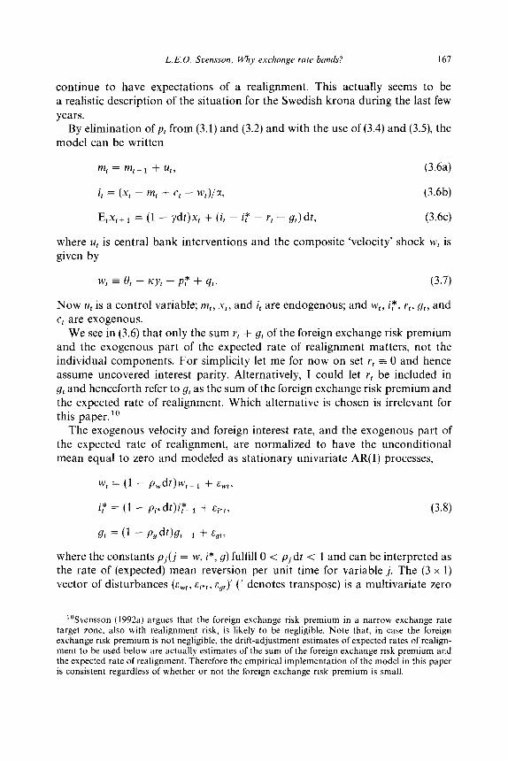
L.E.O. Svensson, Why exchange rate bands? 167

continue to have expectations of a realignment. This actually seems to be a realistic description of the situation for the Swedish krona during the last few

years. By elimination of pt from (3.1) and (3.2) and with the use of (3.4) and (3.9, the

model can be written

m, = mtml + u,, (3.6a)

i, = (x, - m, + c, - w,)/x, (3.6b)

W,+I = (1 - ydt)x, + (i, - i: - r, - gt) dt,

where U, is central bank interventions and the composite ‘velocity’ shock w, is given by

W, = 8, - Kyt - /I; + qt. (3.7)

Now u, is a control variable; m,, x,, and i, are endogenous; and w,, i;“, r,, gt, and c, are exogenous.

We see in (3.6) that only the sum rt + g1 of the foreign exchange risk premium and the exogenous part of the expected rate of realignment matters, not the individual components. For simplicity let me for now on set r, z 0 and hence assume uncovered interest parity. Alternatively, I could let rt be included in gt and henceforth refer to gr as the sum of the foreign exchange risk premium and the expected rate of realignment. Which alternative is chosen is irrelevant for this paper. ’ O

The exogenous velocity and foreign interest rate, and the exogenous part of the expected rate of realignment, are normalized to have the unconditional mean equal to zero and modeled as stationary univariate AR(l) processes,

w, = (1 - Pwdt)w,- 1 + &,t,

i:: = (1 - pi* dt)i,*_ 1 + Ei*t,

st = (1 - Psdt)g,-1 + s,,>

(3.8)

where the constants pj(j = w, i*, g) fulfill 0 < Pj dt < 1 and can be interpreted as the rate of (expected) mean reversion per unit time for variable j. The (3 x 1) vector of disturbances (E,,,~, .sief, egt)) (’ denotes transpose) is a multivariate zero

“Svensson (1992a) argues that the foreign exchange risk premium in a narrow exchange rate target zone, also with realignment risk, is likely to be negligible. Note that, in case the foreign exchange risk premium is not negligible, the drift-adjustment estimates of expected rates of realign- ment to be used below are actually estimates of the sum of the foreign exchange risk premium and the expected rate of realignment. Therefore the empirical implementation of the model in this paper is consistent regardless of whether or not the foreign exchange risk premium is small.

168 L.E.O. Svensson. Why exchange rate bands,?

mean white noise process with variances and covariances denoted by var[sjt] = of dt, cov[sjt, skt] = oj,dt, (j,k = W, i*, 9).

It remains to specify the central bank’s preferences, in line with the focus on interest rate smoothing, and in order to specify the tradeoff between interest rate variability and exchange rate variability (or implicit bandwidth). Therefore I allow the central bank to have several competing targets with interventions in the money supply as the only instrument. By varying the weights on these separate targets the relevant tradeoffs can be found. Consequently, one target is to minimize the exchange rate’s ‘level’ variability: more precisely the expected discounted sum of squared future exchange rates relative to central parity. A second target is to minimize the domestic interest rate’s level variability, more precisely the expected discounted sum of squared future interest rate deviations from the interest rate’s long-run mean. A third target is to minimize the exchange rate’s one-period ‘weekly’ variability, more precisely the expected discounted sum of squared future weekly exchanges in the exchange rate relative to central parity (the unit period dt will be one week in the empirical implemen- tation of the model). A fourth target is to minimize the domestic interest rate’s weekly variability, more precisely the expected discounted sum of squared future weekly changes in the interest rate. A fifth target, finally, is to minimize the interventions, more precisely the expected discounted sum of squared future weekly changes in the money supply. The overall objective is then to minimize a weighted sum of these five targets. Since the focus is on interest and exchange rate stabilization and not on inflation and output stabilization, the latter targets are not included.

This setup gives sufficient flexibility for the present purpose. ‘Interest rate smoothing’ can then be interpreted as referring to both level and weekly variability of the interest rate [cf. Goodfriend (1987, 1991)]. Similarly, ‘exchange rate stability’ refers both to level and weekly variability of the exchange rate relative to central parity [cf. Horngren and Lindberg (1992)]. By varying the weights the five-dimensional tradeoff between the targets can be traced out. In fact I shall concentrate on the tradeoff between level variability of the interest rate and the exchange rate relative to central parity, although the weights on weekly variability of the interest rate and the exchange rate relative to central parity will in some cases be important for that tradeoff. The weight put on minimizing interventions can either be interpreted as representing an actual intervention cost (in which case the weight is bound to be very small) or just representing the central bank’s aversion to interventions (in which case the weight could be large). In the actual computations below, however, the weight on interventions will be zer0.r’

“Since the weight on interventions is set equal to zero, there is no need to discuss what precise measure of interventions the central bank may be concerned about, like frequency of separate interventions, gross or net volume per unit of time, etc.

L.E.O. Svensson, Why exchange rate bands? 169

It is practical to introduce the notation

x, E(Wt,i;F,St,rn,-1,x,-l,i,-1)’ (3.9)

for the (6 x 1) vector of the six predetermined variables at time t. The optimal value of the optimization problem can then be written

+ q&f - i,p ,)‘/dt + q,u:/dt] dt 1 (3.10)

where the minimization is subject to (3.6) and (3.8) and X1 is given [note that (3.5) has been incorporated in (3.6) and is therefore not a separate restriction]. In (3.10), p(O < p < 1) is a discount factor; qj 2 0 (j = x, i, dx, Ai, u) are given weights. The first-differences are scaled by l/dt, and the whole objective function by dt, to make them (approximately) invariant to changes in the period length dt. We exploit that the unconditional mean of the home currency interest rate is equal to zero by the normalization of the exogenous variables.

This is a standard linear-quadratic problem, except that one component, x,, of the state-variable vector is not predetermined but forward-looking and depends on expected future variables. A solution to that variant of the linear-quadratic problem is presented in Backus and Driffill (1986), and their solution is used here. Details are reported in appendix 1.

Commitment vs. discretion

With forward-looking variables in optimization problems ‘time-consistency’ problems usually arise, and this is the case here. Indeed, the solution depends on whether or not the central bank can commit itself to a rule for its interventions. If the central bank can commit to a rule, (3.6) and (3.8) are the only constraints for the problem. Under this situation, ‘commitment’, the optimal intervention policy can be shown to imply that the interventions in future periods t, u,, will be a (linear) function of the predetermined variables in period t, X,, and the exchange rate relative to central parity in period t, x,.

If there is no commitment technology by which the central bank can commit itself to follow the rule, after the first period the central bank usually has an incentive to exercise its right to deviate from the rule, reoptimize, and announce a new rule. This is one example of ‘time-inconsistent’ behaviour. Thus, in the absence of a commitment technology, under ‘discretion’ the central bank re- optimizes each period. Intuitively, we can say that the central bank chooses each

170 L.E.O. Svensson, Why exchange rate bands?

period the exchange rate to minimize its objective function, regardless of what it has previously announced and promised to do. As a consequence the interven- tions in each period can no longer depend on the exchange rate, but only on the predetermined variables in that period. In particular, the exchange rate relative to central parity will be a function only of the predetermined variables in that period. In a rational expectations equilibrium, private agents’ expectations incorporate this restriction. It follows that the forward-looking variables for this period will only depend on this period’s predetermined variables, and that expectations of the next period’s forward-looking variables will only depend on expectations about the next periods predetermined variables. Formally, this means that under discretion the restriction

E,x,+ 1 = CE,X,+ 1 and x, = CX, (3.11)

will be imposed in addition to (3.6) and (3.8) where the endogenous matrix C in our case is a 1 x 6 row vector (in the linear-quadratic framework the dependence is linear). The solution is reported in Oudiz and Sachs (1985) and Backus and Driffill (1986), and reproduced in appendix 1.

Since there are no apparent ways in which a central bank can commit to a particular intervention rule with regard to its interventions within the ex- change rate band, I find the discretion case more realistic and relevant. There- fore the treatment below will concentrate on the discretion solutions and only briefly mention the commitment solutions. l2

4. Results: The trade off between exchange rate and interest rate variability

4.1. Parameters

The parameter values are displayed in table 1. The period length dt is one week. The parameter CY is set equal to 0.5 year. Estimates of it in target zone models are imprecise and fall in the interval from 0.1 to 1 [see Flood, Rose, and Mathieson (1991) and Lindberg and Soderlind (1992)]. The results here do not seem sensitive to some variation in a, say between 0.2 and 1. Even though the model uses weekly interest rates, interest rates of any maturity are easily derived with the expectations hypothesis for the term structure of interest rates (see appendix 2). To facilitate comparison with actual one-month interest rates I shall report results for four-week interest rates (it is practical to choose the

“Note that the time-consistency problem discussed here concerns the intervention policy within the band, rather than the much discussed time-consistency problem with respect to the realignment policy.

L.E.O. Svensson. Wh_v exchange rate bands? 171

Table 1

Parameter values.

dt = l/52 year

r = 0.5 year

z = 4 weeks

pW = 0.2 per year

p,. = 0.417 per year

ps = 5.14 per year

1 - p,dt = 0.996

1 - pi.dt = 0.992

1 - psdt = 0.901

0:. = 15 basis points (0.15 percent) per year

o,? = 1.64 basis points per year3

c$ = 74.2 basis points per year3

cjj = 0 (i, j = w, i*, g, i fj)

y = 0,0.7, or 1.4 per year

/I = 0.9 (annualized), 8”’ = 0.9980

4” = 0

maturity an integer multiple of the period length). The constant z, the maturity in periods, is therefore set equal to four.

The rate of mean reversion ~7 and the rate of variance c’* for i: are equal to estimates from a univariate AR(l) regression (with one week’s lag) on a one- month currency basket interest rate (sample period January 1986 to February 1992; Swedish krona basket weights of one-month Euro interest rates before May 17,1991, when Sweden switched to an ecu basket, thereafter theoretical ecu weights of one-month Euro interest rates). The mean reversion ps and the rate of variance 0.92 of g1 are equal to estimates from a univariate AR(l) regression (with a week’s lag) on one-month expected rates of devaluation of the Swedish krona that have in turn been estimated with the ‘drift-adjustment’ method.‘3,i4 The

13The drift-adjustment method was suggested by Bertola and Svensson (1993), and empirically implicated by Rose and Svensson (1991) and Lindberg, Stiderlind, and Svensson (1993).

14The estimated variances in the AR(l) regressions are divided by df in order to be expressed as rates of variances, and scaled by the factor [(l - (1 - pjdt)‘)/(sp,dt)]’ (for j = i*, g) in order to apply to one-week interest rates and expected rates of realignment (see appendix 2).

In the first stage of the drift-adjustment estimates of expected rates of realignment, the estimated expected rates of depreciation relative to central parity are found to depend not only on the current exchange rate’s deviation from central parity but also on the one-month domestic and foreign interest rates. This finding is different from that of Lindberg, Sdderlind, and Svensson (1993) and seems to be the result of the current sample including more recent observations.

172 L.E.O. Suensson, Why exchange rate bands?

parameters p,,, and gi for w, are a guess, but these parameters do not affect the results since the interventions, as we shall see, will always cancel the effect of w, (as long as intervention costs are zero). The AR(l) coefficients for w,, i:, and gt(l - pjdt, j = w, i*, g) are also reported in table 1. The rates of covariance between the exogenous variables are for simplicity set equal to zero.

Three values of y, the sensitivity of the expected rate of realignment to the exchange rate’s deviation from central parity, are used: 0, 0.7 per year, and 1.4 per year. Empirical estimation of y in (3.5) results in an identification problem since the exchange rate is correlated with the expected rate of realignment even if y is zero. An OLS as well as an instrumental variables regression of drift- adjustment estimated expected rates of realignment on the exchange rate results in an estimate of y equal to about 1.4 per year; this could be interpreted as providing an upper limit since then all of the covariation of the exchange rate and the expected rate of realignment is attributed to y.

The annualized discount factor fl is set to 0.9, which corresponds to

B . r”’ = 0 9980 for a week. The objective function weight q,, on interventions is set equal to zero, corresponding to the assumption that intervention costs are negligible and that the central bank has no aversion to intervening. As we shall see, the resulting interventions are rather modest compared to reasonable measures of actual interventions. A small positive weight does not change results much. A large weight implies that the parameters and realization of the stochas- tic process for w, will significantly affect the solution.

4.2. The tradeof between exchange rate and interest rate level variability

The tradeoff between theoretical unconditional level standard deviations [that is, computed via (A.26) and (A.27) or (A.41) in appendix l] of the exchange rate and four-week interest rate is illustrated in fig. 1. The thick curve refers to commitment, the thin curves to discretion. Solid curves refer to the case when y = 0, that is, when the expected rate of realignment is independent of the exchange rate’s deviation from central parity. Long dashes refer to the case when y = 0.7 per year, and short dashes refer to the (upper-limit) case when y = 1.4 per year. Markers like C3.3 and D3.2 refer to Commitment case (3.3) and Discretion case (3.2), where the objective function weights and the value of y for the different cases are reported in table 2. The actual empirical standard deviations of the Swedish krona exchange rate and the one-month Swedish krona Euro interest rate for the sample period January 1986 to February 1992 are marked by A. The corresponding standard deviations of the exchange rate and the interest rate are at the lower left corner of each marker.

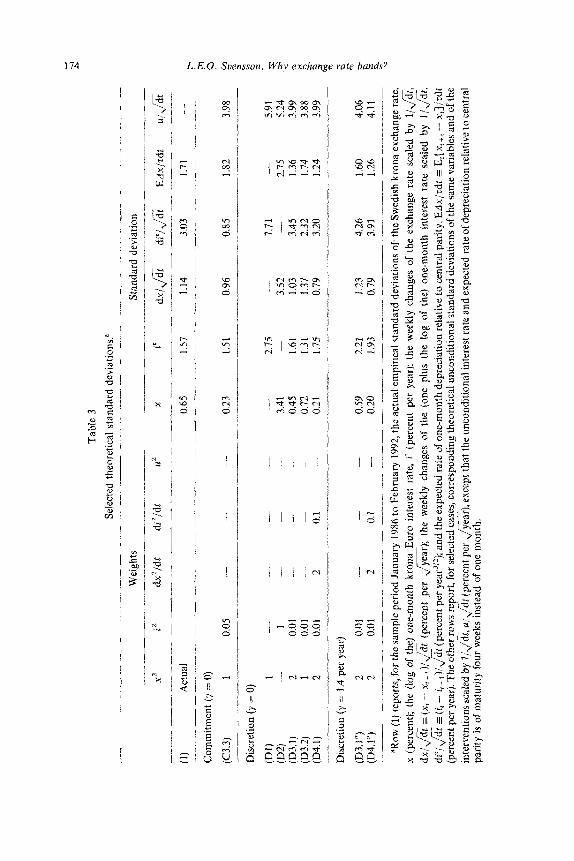
Table 3 reports for selected cases the theoretical unconditional standard deviations of the exchange rate, x, (percent), the four-week interest rate,

ii (percent per year), the weekly changes of the exchange rate scaled by l/Jdt,

L.E.O. Sumsson, Why e.uchange rate bands? 173

32

,D3 2” 28 /

, /

/ ,

24 / /

- Commitment y=o - Dlscretlon y”=o

- - Dlscretlon r=o 7/yr

_-- Dlrcretion r= 1 4/yr !

Fig. 1. The tradeoff between exchange rate (x) and interest rate (i’) standard deviations; A = actual standard deviations.

Table 2

List of cases in fig. 1.

(1) (2) (3.1)

(3.1’) (3.1”) (3.2) (3.2’) (3.2”) (3.3) (3.3’) (4.1)

(4.1”)

X2

1

2

2 2 1 1 1 1 1 2

2

i2

1 0.01

0.01 0.01 0.01 0.01 0.01 0.05 0.05 0.01

0.01

Weights dx=ldt

-

- -

-

2

2

di’ldt

0.1

0.1

u2

-

- -

-

- - -

(per ;ear)

0.7 1.4

0.7 1.4

1.4 - 1.4

dxl&t 3 (x, - x,_ 1 )/&it (p ercent per &), the weekly changes of the

four-week interest rate scaled by I/$, di’/Jdt = (it - it_ ,)/$ (percent per year3’2), the expected rate of four-week expected depreciation relative to central parity, Edx/z = Et[xt+r - xt]/Tdt (percent per year), and the interventions

Tab

le 3

Sele

cted

the

oret

ical

st

anda

rd

devi

atio

ns.’

_

_ _

-_._

_ ___

_I__

_

~_

_ __

__

l.l..”

_

- ._

-._

- _l

__-

__._

~

Wei

ghts

St

anda

rd

devi

atio

n ._

-__

----

- _.

.. l.l

”.-_

_-_l

--

_ -_

--

____

-,__

_

X2

i2

dxZ

/dr

dP/&

u=

X

i’

f

dxj.,

, dt

di

r/,/%

E

dxJr

dc

u/J&

_,

^__

~.

___

____

__ _

~_

_ __

.__

_ _

._.“

.___

. _~

____

_-_.

^_ _

.._ __

--

._

.__

- -

~I._

-.

___

.-_

____

___

(1)

Act

ual

0.65

1.

57

1.14

3.

03

1.71

-

___

~ __

~ _

____

~^

__

_ -.

ll_l_

-_

- __

___-

.--

-

--

_.-_

____

-.

-.-.

_ ._

-

.- __

.__

(C3.

3)

1 0.

05

--

- -

0.23

1.

51

0.96

0.

85

1.82

3.

98

~_--

~ ~-

_-

--__

_ --

~ __

l_l_

--

----

- -l

..-__

_

Dis

cret

ion

(r =

0)

I;$

1 -

- -

- -.

_ 2.

75

- 7.

71

- 5.

91

_._-

1

_^_

- 3.

41

- 3.

52

--~

2.75

5.

24

(D3.

1)

2 0.

01

- -

- 0.

45

1.61

L

O3

3.45

1.

36

3.99

(l

I3.2

) :

0.01

-

- 0.

72

1.31

1.

37

2.32

1.

74

3.88

(D

4.1)

0.

01

2 0.

1 -

0.21

1.

75

0.79

3.

20

1.24

3.

99

- ~-

- -_

____

-l_l

l-.-

~-__

---,

.-_

Dis

cret

ion

Ip =

I.4

per

yea

r)

Com

mitm

ent

(7 =

0)

(D3.

1”)

2 0.

01

--

- -

0.59

2.

21

1.23

4.

26

1.60

4.

06

(D4.

1”)

2 0.

01

2 0.

1 -

O*2

0 1.

93

0.79

3.

91

1.26

4.

11

_ ._

_ -_

l-_l

”__

._

_I

--.

--~

-. _1

^1.-

- .-.

__

__

.---

--.-

-

“Row

(1)

repo

rts,

for

the

sam

ple

peri

od J

anua

ry

1986

to F

ebru

ary

1992

, the

act

ual

empi

rica

l st

anda

rd

devi

atio

ns

of: t

he S

wed

ish

kron

a ex

chan

ge r

ate,

x

(per

cent

);

the

(lag

of

the)

one

-mon

th

kron

a E

uro

inte

rest

ra

te,

i’ (

perc

ent

pet

year

); t

he

wee

kly

chan

ges

of t

he

exch

ange

ra

te

scal

ed

by

l/J&

, dx

/&

E (

x, -

xI

__ L

)j.&

(p

erce

nt

per

,&};

th

e w

eekl

y ch

ange

s of

the

(o

ne

plus

th

e lo

g of

the

) on

e-m

onth

in

tere

st

rate

sc

aled

by

l/J

&,

dir/

,/&

= (

i, -

ii- ,

)/$%

(p

erce

nt

per

year

3’2]

; and

the

exp

ecte

d ra

te o

f o

ne-

mo

nth

dep

reci

atio

n re

lativ

e to

cen

tral

par

ity,

lEdx

]sdt

z

E,[

x~,.,

-

x,tjz

ddr

(per

cent

per

yea

r). T

he o

ther

row

s re

port

, fo

r se

lect

ed c

ases

, co

rres

pond

ing

theo

retic

al

unco

nditi

onal

st

anda

rd

devi

atio

ns

of th

e sa

me

vari

able

s an

d of

the

inte

rven

tions

sc

aled

by

l/,/&

u/,/%

(p

erce

nt p

er &

),

exce

pt t

hat

the

unco

nditi

onal

in

tere

st r

ate

and

expe

cted

rat

e of

dep

reci

atio

n re

lativ

e to

cen

tral

pa

rity

is

of m

atur

ity

four

wee

ks i

nste

ad

of o

ne m

onth

.

L.E.O. Svensson. Why exchange rate bands? 175

scaled by l/a, u/& (percent per 6)” Row 1 in table 3 reports the actual empirical standard deviations for the sample period January 1986 to February 1992 (one-month instead of four-week interest rate). The other rows report the theoretical standard deviations for selected cases.

The implicit band for the exchange rate can be operationally defined as +3 times its standard deviation, that is, k3.0.65 = _+ 1.95 percent for the actual exchange rate. The probability of being outside this band is (for a normally distributed exchange rate) a meager 0.27 percent, which on the average would occur on less than five days of the approximately 1600 market days in the six years and two months long sample.16

Let us return to fig. 1. Let us first consider the situation when the expected rate of realignment does not depend on the exchange rate relative to central parity (y = 0). The thick solid curve shows the tradeoff under commitment, when the central bank gives weight to the variability of exchange rate and interest rate levels only but not to the weekly variability. The thin solid curve shows the tradeoff under the same conditions but under discretion. Except at the edges, the think curve is above and to the right of the thick curve; the tradeoff under discretion is less favorable than under commitment. The actual standard deviations (marked by A) are outside both curves; an optimal intervention policy can reduce the standard deviations of both the exchange rate and the interest rate, also under discretion. Commitment case C3.3 can reduce the exchange rate standard deviation from the actual 0.65 percent by about 2/3 to 0.23 percent (from an implicit exchange rate band of + 1.95 percent to kO.69 percent), at roughly unchanged interest rate standard deviation. Discretion case D3.1 can reduce the exchange rate standard deviation by l/3 to 0.45 percent (the implicit band from + 1.95 percent to _+ 1.35 percent), at roughly unchanged interest rate standard deviation.

Discretion not only makes the tradeoff less favorable than commitment; for given objective function weights it also biases the tradeoff against exchange rate variability. We see this by comparing, for instance, commitment case C3.3 with discretion case D3.3, which both have the same weights on exchange rate and interest rate variability, qX = 4i = 1. The discretion case results in much larger exchange rate standard deviation and lower interest rate standard deviation.

l5The weekly changes and the interventions are scaled by l/J& because the corresponding variances are then linear in the period length. The scaling has the practical advantage that the variances and standard deviations are of the same order of magnitude.

r6Lindberg and Soderlind (1992) cannot reject the hypothesis that the unconditional distribution of the Swedish krona’s deviation from central parity is normal. Note also that the standard deviation of a normal distribution that is truncated beyond 13 standard deviations is 98.5 percent of the untruncated distribution’s standard deviation, so the bias in reported standard deviations caused by the approximation is negligible.

176 L.E.O. Soensson, Why exchange rate bands?

4.3. The extreme cases

At the edges, the commitment and discretion cases coincide. The exchange rate can be completely stabilized with an interest standard deviation of 2.75 percent per year (Cl = Dl). The interest rate can be completely stabilized to its long-run mean with an exchange rate standard deviation of 3.41 percent, that is, an implicit exchange rate band of about + 10 percent (C2 = D2).

Understanding the extreme cases at the edges is the clue to an intuitive understanding of the results reported above and of the optimal intervention policy. Let us therefore consider these cases more thoroughly. Fortunately, these cases have simple closed form solutions: We rewrite (3.6b)-(3.6c) as

1 x, = ___ h, + a E,[x,+~ - x,]/dt

1 + ccy 1 + ay

1 h +

a/dt

= 1 + a/dt - ccy 1 + a/dt - ay ES,+ I (4.1)

where the (composite) fundamental h, is given by

h, 5 m, + w, + CX($ + gt)

= m,-, + u, + w, + a(iF + gr) (4.2)

(we have set c, = 0), and where we exploited that limj_, E,x,+j equals the unconditional mean E[x,] which is zero. We also note that the interest rate fulfils

i, = i: + g1 + E,[x,+l - x,l/dt. (4.3)

Let us first take case (Cl = Dl) when the exchange rate is constant and equal to zero. It follows from (4.1) that h, must be constant and equal to zero. Hence, from (4.2),

m, = - w, - cc(it* + gt), (4.4)

U, = - w, - cL(i,* + gt) - m,_ 1. (4.5)

It follows that the interventions are simply chosen so as to fully cancel the innovations in w, + a($ + gt).

L.E.O. Swnsson, Why exchange rate bands.? 177

Furthermore, from (4.3) follows that the interest rate is simply given by

i, = i: + gr, (4.6)

the sum of the foreign interest rate and the expected rate of realignment, since the expected rate of depreciation relative to central parity is zero.

In case (C2 = D2) when the interest rate is held constant and equal to zero, it follows from (4.3) that

xc = {i: + E,[c,+ 1 - c,]/dt} dt + E,x,+,

= (i: + yxt + g,)dt + E,x,+l

=$&it + gt)dt + L E,x,+l 1 - ydt (4.7)

= & Et $I0 (&J (iF+j + gt+j)dt

If y < pi* and y < ps, the sums above converge. Then we can write

xt = ifl(Pi* - Y) + gtl(Pg - Y).

From (3.6b) and i, = 0 follows that

(4.8)

m, = - w, + xt = - w, + if/(pi. - y) + g,/(p, - y).

Hence the interventions are given by

(4.9)

U,= -Wwt+i:/pi*+g,/p,--m,-l. (4.10)

The intuition for the two cases (Cl = Dl) and (C2 = D2) is then easy. In case (Cl = Dl), with a constant exchange rate, the interventions simply cancel the shocks to w, + a(ij+ + gt) and are hence strongly ‘leaning-against-the-wind’. With a zero expected rate of depreciation relative to central parity, the interest rate is simply the sum of the foreign interest rate and the expected rate of realignment.

In case (C2 = D2), with a constant interest rate, the interventions still cancel shocks to w,. That is always optimal in all cases as long as intervention costs are zero. But now, from (4.3) we see that an innovation to ij+ + gt must result in an opposite innovation to the expected rate of depreciation relative to central

178 L.E.O. Svensson, Why exchange rate bands.7

parity, in order to hold the domestic interest rate constant. An increase in i* must be countered by a decrease in the expected depreciation relative to central parity. This is achieved by an instantaneous increase of the exchange rate, which decreases the expected future depreciation. The instantaneous increase in the exchange rate requires a positive intervention, that is, an increase in the money supply. Therefore, in (4.10) the interventions are increasing in if and gt, ‘leaning-with-the-wind’. Furthermore, we see in (4.8) and (4.10) that the more persistent the innovations in i: and g1 are (the smaller pi* and ps are), the more ‘overshooting’ there is in the interventions and the exchange rate.

As discussed in section 3, under discretion the current exchange rate and interest rate must only depend on the current predetermined variables. The reason the commitment and discretion cases (Cl = Dl) and (C2 = D2) are identical is that the solution indeed is such that the exchange rate [in case (C2 = D2)] and interest rate [in case (Cl = Dl)] can be written as functions of only the predetermined variables; see (4.6) and (4.8). Put differently, the con- straint (3.11) is not binding. For other objective function weights, the constraint (3.11) is binding under discretion, and the discretion and commitment solutions are different with a less favorable tradeoff between exchange rate and interest rate variability under discretion.

4.4. The expected rate of realignment sensitive to the exchange rate relative to parity

The effect on the tradeoff of a positive y is shown for the discretion case by the curves with long dashes (y = 0.7 per year) and short dashes (y = 1.4 per year). The dashed curves are above the thin curve. As discussed in section 2, intuitively it is more difficult to stabilize the domestic interest rate if expected rates of realignment increase with the exchange rate relative to central parity.17

“Counter to simple intuition, under commitment the tradeoff between interest rate and exchange rate variability actually improves with y. If we had plotted dashed curves for the commitment case they would be below the thick curve, in contrast to the discretion case. Why does y have such different effects under commitment and discretion?

One way to understand this is to look at (3.6~). That equation shows that the central bank can control the nominal interest rate i, by control over the the current exchange rate x, and the expected future exchange rate, E,x, + I. Under commitment the central bank can affect the expected future exchange rate to a considerable extent and use that to control the nominal interest rate. A larger 7 is then an advantage; with a smaller coefficient (1 - ydt) multiplying the current exchange rate, the current exchange rate can be moved around with only a small effect on the nominal interest rate.

Under discretion the central bank has much less power to influence the expected future exchange rate, since that is constrained by (3.11) to depend only on expected future predetermined variables. Let us simplify by taking the expected future exchange rate as given. Then the central bank can only use the current exchange rate to control the interest rate. Now, a larger 7 is a disadvantage; a smaller coefficient (1 - ydt) means that the exchange rate has to be moved more in order to control the nominal interest rate.

L.E.O. Svensson. Why exchange rate bands? 179

In order to completely stabilize the interest rate, y must be less than both pi* and ps, as we noted when deriving (4.8). With our parameters this is not the case for y = 0.7 or 1.4 per year, since pi* = 0.417 per year. Therefore the dashed curves do not intersect the horizontal axis in fig. 1.

4.5. With discretion, more targets can improve the outcome

Fig. 1 and table 3 reveal that, under discretion, adding weights on the weekly variability of exchange rates and interest rates may improve the outcome. Case D4.1 differs from case D3.1 only in that weights on the weekly variabilities have been added, but case D4.1 is much closer to the commitment tradeoff. The improvement from case D3.1” to D4.1” (when y = 1.4 per year) is even larger. This illustrates the complexity in the discretion case. Under discretion there is an inherent nonconvexity in the problem, due to the restriction (3.11). In the commitment problem, adding weights on additional targets make it more difficult to fulfill the initial ones. The opposite may be the case under discretion, as a comparison between D3.1” and D4.1” shows. Let me try to provide some intuition for this.

If only level exchange rate and interest rate variability matters, under discre- tion there is an incentive to deviate and bring the forward-looking exchange rate and interest rates immediately to their long-run means. We shall see this in simulations below, where the optimal exchange rate and interest rate start out at central parity and the long-run mean, respectively, even though the initial values (set equal to the actual historical values) are different. The market understands this incentive, and its incorporation implies a severe restriction on the problem. Now, if the central bank also has targets for weekly exchange rate and interest rate variability, it is less inclined to deviate by suddenly moving the exchange rate and interest rate all the way to their long-run means. Incorporating the incentive therefore implies less of a constraint, and the outcome becomes better. Having more targets is like ‘tying one’s hands’, which often improves the situation when there is a time-consistency problem. Perhaps this result can provide a new justification for the use of intermediate targets, namely as ‘instruments of commitment’.

5. Simulations

Simulations of the Swedish krona target zone are done for the period January 1986 to February 1992. The simulations use the parameters displayed in table 1. As exogenous realizations for the foreign interest rate and expected rate of realignment I use weekly observations of the (log of one plus the) actual one-month foreign interest rate and the drift-adjustment estimated expected rate of realignment, each variable scaled to correspond to one-week interest rates

180 L.E.O. Swnsson. Why exchange rate bands?

and expected rates of realignment.’ * The realizations of the exogenous variable w, are generated, but with zero intervention costs they do not affect the equilibrium aside from the interventions.

The results of the simulations are displayed in table 4 and in five figs. 2a-e, named by the corresponding cases: Dl, D2, . . , D4.1”. Row 1 in table 4 shows the actual empirical standard deviations. The other rows show, for the different cases, the simulated standard deviations, the sample standard deviations of the series generated by the simulations [rather than the theoretical unconditional standard deviations in table 3 and fig. 1 generated by (A.22) with (A.26) and (A.41) in appendix 11. The figures show for each case the exchange rate deviation from the central parity, x, with the + 1.5 percent band (percent; thin curve: actual empirical; thick curve: optimal simulated); the (log of one plus the) domestic-currency interest rate, i’ (percent per year; thin curve: actual one- month krona Euro rate; thick curve: optimal four-week krona rate); the (log of one plus the) foreign-currency interest rate, i*r (percent per year; one-month weighted Euro rate); the expected rate of realignment, g’ (percent per year; thin curve: actual four-week exogenous part; when y is positive: medium curve: actual total four-week expected rate of realignment, thick curve: optimal four-week expected rate of realignment); the expected rate of depreciation relative to central parity, E,[x,+, - x,]/zdt (percent per year; thin curve: actual one-

month; thick curve: optimal four-week); and the innovations scaled by l/Jdt,

U/G (percent per 6). First we consider simulations when the expected rate of realignment does not

depend on the exchange rate (y = 0). Fig. 2a, discretion case Dl (which coincides with commitment case Cl), with weight only on exchange rate variance, has a completely fixed exchange rate. The krona interest rate is the sum of the foreign interest rate and the expected rate of realignment. Its standard deviation is larger than the actual. The interventions are strongly leaning-towards-the- wind. Some fairly large interventions are needed to counter the increase in the expected rate of realignment in early and late 1990.

Before going further, let us consider what a realistic intervention size is. Take

a large intervention in fig. 2a, u,Jfi = 20 percent/&, which corresponds

to u, = 0.2/a z 2.8 percent. What is a typical real world intervention? It is not obvious how to measure actual interventions and open market operations and translate these into the framework of this model [see Lindberg and Soderlind (1992)]. One possibility is to use weekly changes in the monetary base. The Swedish monetary base is around 200 billion kronor (about $33 billion around 1990). A weekly change of 20 billion kronor is not rare. Such a 10 percent change should be compared to the 2.8 percent change derived above.

‘*See footnote 15 for the scaling factors

Tab

le

4

Sim

ulat

ed

stan

dard

de

viat

ions

.”

__~

~-~

x2

iz

(1)

Act

ual

Dis

cret

ion

(y =

0)

Wei

ghts

St

anda

rd

devi

atio

n .~

d.x*

jdt

di’l

dt

U2

x

i’ d

xJJ;

i;

dir/

,,&

EA

x/T

dt

ulfi

-~

__

~__~

__

~

0.65

1.

57

1.14

3.

03

1.71

__

_

(Dl)

1

_ 2.

55

7.16

-

5.63

(D

2)

1 2.

86

3.06

2.

55

5.12

(D

3.1)

2

0.0

1 0.

40

1.41

0.

9 1

3.00

1.

35

3.88

(D

4.1)

2

0.01

2

0.1

_ 0.

22

1.57

0.

72

0.72

1.

25

4.01

_~

__

~___

~_

_ ~_

__

--__

Dis

cret

ion

(;I =

1.

4 pe

r ye

ar)

(D4.

1”)

2 0.

01

2 0.

1 0.

19

1.46

0.

68

3.30

1.

15

~ -~

__

~__

-~

__

“See

not

e to

ta

ble

3, e

xcep

t th

at

row

s ot

her

than

ro

w

(I)

refe

r to

si

mul

ated

ra

ther

th

an

theo

retic

al

unco

nditi

onal

st

anda

rd

devi

atio

ns.

4.09

182 L.E.O. Svmsson, Why exchange rate bands?

87 88 a9 90 91 92 53

07 88 89 90 91 92 43

-&? I37 88 89 90 91 92 53

0

“B 87 88 89 90 91 92 63

I

86 87 88 89 90 91 92 §3

Fig. 2a. Case D1 = Cl. qx = 1.00, qi = 0.00, qdx = 0.00, qd, = 0.00, 4. = 0.00, y = O.O/year, 5 = 4 weeks; thin curve = actual, thick curve = optimal, dashed line = mean.

Such a comparison leads me to believe that the intervention sizes that result in the simulations are not larger than actual ones, even though a zero objective function weight on interventions is assumed.

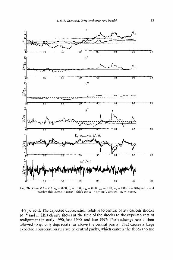
Fig. 2b, discretion case D2 (which coincides with commitment case C2), with weight only on interest rate variance, has a completely fixed interest rate. This requires a much wider implicit exchange rate band than the actual one, almost

L.E.O. Scensson, Why exchange rate bands? 183

a7 88 69 90 91 92 g3

*

67 88 69 90 91 92 G3

3

I 8 67 68 89 90 91 92 53

Fig. 2b. Case I)2 = C2. yx = 0.00, qi = 1.00, qnx = 0.00, qdi = 0.00, qu = 0.00, 7 = O.O/year, ‘L = 4 weeks; thin curve = actual, thick curve = optimal, dashed line = mean.

rt 9 percent. The expected depreciation relative to central parity cancels shocks to i* and LJ. This clearly shows at the time of the shocks to the expected rate of realignment in early 1990, late 1990, and late 1992: The exchange rate is then allowed to quickly depreciate far above the central parity. That causes a large expected appreciation relative to central parity, which cancels the shocks to the

tl7 88 09 90 91 $ja §3

.*T z

3

86 87 88 89 90 9t 92 ?a

Fig. 2c. Case 03.1. 4% = 2.00, qL = 0.01, qdlr: = 0.00, qni = 0.00, qU = 0.00,~ = O.O/year, T = 4 weeks; thin curve = actual, thick curve = optimal, dashed line = mean.

expected rate of realignment and keeps the nominal interest rate constant. Interventions are leaning-with-t~~~~ind for shocks to i* and g.

Fig. 2c, discretion case D3.1, is a considerable improvement upon the actual historical outcome. The variability for both the exchange rate and the interest rate are lower (see table 4). In fig. 2d, discretion case D4.1, weights on the weekly variability of the exchange rate and interest rate are added. This remits in less

L.E.O. Svensson, Why exchange rate bands? 185

87 88 BY 90 91 92 53

w k-

-A RO

736 a7 88 a9 90 91 92 §3

a8

0

7% 87 a8 a9 90 91 92 §3

a7 a8 a9 90 91 92 3

Fig. 2d. Case 04.1. qx = 2.00, qi = 0.01, qnz = 2.00, qdi = 0.10, qu = 0.00, y = O.O/year, T = 4 weeks; thin curve = actual, thick curve = optimal, dashed line = mean.

variability of the exchange rate and a somewhat farger variability of the interest rate. Compared to the actual case, the exchange rate standard deviation is only a third, without any increase in the interest rate standard deviation. This illustrates that, under discretion, having more targets may improve the outcome, as we discussed in section 3.

186 L.E.O. Svensson, Why exchange rate bands?

The simulations show that the incentive to deviate by moving the exchange rate and interest rate immediately to their long-run means is weakened by weights on weekly variability of the exchange rates and interest rate: When there is no weight on weekly exchange rate and interest rate variability, as in fig. 2c, case D3.1, the optimal exchange rate and interest rate starts out from zero (at period 1, the first week of 1986) even if the predetermined values (set equal to the

-& a7 aa a9 90 91 92 53

i’,

%6 a7 aa 69 90 Yl 92 93

2 I

g’ (Thin) Et[~t+,-c~]/~dt (Medium: actual, Thick: optimal)

II

3

‘Uxt+T -ZJ/7&

a7 88 as 90 91 92 53

1 86 a7 68 09 90 91 92 53

Fig. 2e. Case 04.1”. qx = 2.00, q3 = 0.01, qnx = 2.00, qdi = 0.10, q. = 0.00, y = 1.4/year, 5 = 4 weeks; thin curve = actual, thick curve = optimal, dashed line = mean.

L.E.O. Svensson. Why exchange rate bands? 187

actual exchange rate and interest rate in period 1) are very different. When there is a weight on weekly variabilities, as in fig. 2d, case D4.1, the optimal exchange rate and interest rate no longer start at zero but are affected by the predeter- mined values.

A comparison between the simulated standard deviations in table 4 and the theoretical ones in table 3 reveals that in several cases the simulated standard deviations are smaller than the theoretical. This indicates that the theoretical tradeoffs in fig. 1 may be a bit biased towards being less favorable than the ‘true’ tradeoff.

There are some conspicuous deviations between the actual outcome for the exchange rate and interest rate and the simulated optimal outcome for different objective weights. One such deviation is in 1989, when the actual exchange rate was lower and the nominal interest rate was higher than the simulated (see for instance fig. 2d). Sveriges Riksbank has publicly declared that it indeed con- sciously kept the krona strong during that period in order to induce a high domestic interest rate to counter the overheating of the Swedish economy at the time. Another such deviation may be evident in the second half of 1991, when the krona was kept rather week, possibly in an attempt to induce a low domestic interest rate to counter the recent recession in the Swedish economy. Indeed, the actual domestic interest rate was lower than the optimal one during this period, although not by very much. These instances indicate that there are probably other targets for the central bank than to stabilize domestic interest rates, for instance to stabilize output or inflation.

Interestingly, the effect on the domestic interest rate of such deviations of the exchange rate from the optimal solutions is dampened if the expected rates of realignment are sensitive to the exchange rate’s deviation from central parity. This is apparent in fig. 2e, case D4.1” (with y = 1.4 per year), where the difference between the actual and optimal exchange rate during 1989 is smaller than in fig. 2d (with y = 0). Naturally, with a positive y a strong krona reduces the expected rate of realignment which reduces the domestic interest rate.

6. Conclusions, qualifications, and extensions

The paper has examined the amount of monetary independence that arises in an exchange rate band. The monetary independence arises since the central bank has some control over the domestic(-currency) interest rate. The central bank can exercise this control by allowing exchange rate movements within the band that result in an expected rate of future depreciation relative to central parity that is consistent with a desired level of the domestic interest rate. The control over the domestic interest rate is limited to short-maturity interest rates and to short-term fluctuations in these interest rates. The monetary indepen- dence can be exploited in different ways, for instance in order to stabilize output,

188 L.E.O. Svensson, Wh_v exchange rate bands?

inflation, or the domestic interest rate (interest rate smoothing). The paper has focused on the last possibility, and has specified the tradeoff between exchange rate and interest rate variability. A wider exchange rate band allows the central bank to reduce domestic interest rate variability.

’ The tradeoff between exchange rate and interest rate variability is less favor- able if the central bank cannot commit to an intervention policy rule, that is, under ‘discretion’. Even so, for realistic parameters fig. 1 (for instance case D3.2 in table 3, or even the actual outcome marked by A) shows that under discretion the central bank can reduce the standard deviation of the domestic interest rate by about a half by increasing the exchange rate standard deviation from zero to about 0.7 percent (that is, by extending the implicit exchange rate band from zero to about k 2 percent around central parity). If the central bank gives weight to the weekly stability of exchange rate and interest rate, the tradeoff under discretion improves and may be close to the favorable tradeoff under commitment. If expected rates of realignment are sensitive to the exchange rate’s position in the band, the amount of monetary independence is reduced. How- ever, with weights on weekly stability of the exchange rate and interest rate the monetary independence may still be sizable.

The intuition for the intervention policy is fairly straightforward: The central bank should always lean strongly against the wind for all shocks excepts shocks to the foreign interest rate, to the expected rate of realignment, and to the foreign exchange risk premium. If the central bank is mainly concerned about reducing exchange rate variability, it should lean against the wind also for these latter shocks. If the central bank is mainly concerned about reducing interest rate variability, it should lean with the wind for these latter shocks, in order to depreciate the current exchange rate and create an expected future depreciation of the exchange rate relative to central parity that dampens the shock to the domestic interest rate.

The monetary independence arises since the central bank can exploit the mean reversion of the exchange rate relative to central parity. As noticed by Horngren and Lindberg (1992) this is an interesting example of the character- istic of successful central banks that is emphasized in Bernanke and Mishkin’s (1992) survey of a monetary policy in six countries. According to Bernanke and Mishkin successful central banks have long-term credibility in the form of an expected long-run mean reversion of the monetary variables the banks are concerned about. This long-run credibility give the banks considerable short- term discretion. As we have seen, an exchange rate band may give a similar combination of long-run mean reversion and short-run discretion.

I found the amount of monetary independence in an exchange rate band to be larger than I anticipated when I started working on this paper. Although I believe that this monetary independence is probably the best explanation why central banks prefer current-size bands to (almost) zero bands, I hasten to add that it does not follow that central banks should exploit the monetary

L.E.O. Svensson. Why exchange rate bands? 189

independence available in an exchange rate band. First, the monetary indepen- dence that I have chosen to quantify only concerns interest rate smoothing. Even if interest rate smoothing may be a realistic assumption about central bank behavior, it is by no means clear that interest rate smoothing is a socially desirable objective. In order to judge that, the real effects of interest rate smoothing need to be established. Second, interest rate smoothing is not the only concern of central banks; they are often directly concerned about the real effects of their policies on investment, output, and employment. Hence this also asks for an explicit study of the real monetary independence that may result from exchange rate band, in the sense of influence over real variables, which as mentioned is a desirable future extension of the present framework. It may be that what appears as a sizable monetary independence with regard to the domestic interest rate actually has insignificant effects on real variables. Third, it may be that expected rates of realignment are related in a complex way to the intervention policy within the band. The Austrian and Dutch central banks have in recent years conspicuously abstained from exploiting any monetary indepen- dence and kept their exchange rates very close to central parities relative to the Deutsche mark. After that policy was instituted, interest rate differentials rela- tive to the Deutsche mark have all but vanished, and drift-adjustment estimates of expected rates of realignment against the Deutsche mark are not significantly different from zero. Thus, voluntarily abstaining from exploiting the monetary independence in an exchange rate band may in some cases contribute to increasing the credibility of the exchange rate band.”

The analysis presumes that the different shocks can be identified by the central bank and market participants. Foreign interest rates are directly observ- able, and the sum of expected rate of realignment and the foreign exchange risk premium (if any) can be estimated day-by-day with the drift-adjustment method. What about the third shock in the model, the composite velocity shock? This shock can be interpreted as a shock to the liquidity of the banking system. Forecasting changes in liquidity and countering them by repurchase agreement and open market operations is part of the daily routine at Sveriges Riksbank. Private banks also routinely forecast liquidity shocks in order to plan their overnight balances. The assumption of observability of the third shock is therefore perhaps not farfetched. Nevertheless, the shocks to composite velocity and the expected rate of realignment may not be perfectly observable, and a possible future extension of the model is certainly to consider imperfectly observed shocks, for instance with Kalman filter methods.

We should recall that the managed float model without explicit bands and without any marginal interventions used here is only an approximation to

190n the other hand, Sveriges Riksbank has kept the krona very close to its central parity since spring 1992, which did not prevent the speculative attacks and eventual collapse of the fixed exchange rate regime in November 1992.

190 L.E.O. Svensson. Why exchange rate bands?

a situation with explicit band and with marginal interventions. It remains to be seen if future work beyond Lindberg and Siiderlind (1992) will support the goodness of the approximation, although that seems rather likely.

Among possible extensions, it should be possible to do a Generalized Method of Moments estimation of the parameters of the model. Even a Maximum Likelihood estimation may be feasible, since the linearity of the model will imply normal distributions as long as the exogenous shocks are normal. It should be possible to infer the implicit weights in central bank objective functions and the resulting optimal intervention policy. Having access to actual intervention data would of course be extremely useful.

It is already clear from the model that the optimal intervention policy generally is more complicated than simple leaning towards the wind. This implies that the modeling of intramarginal interventions in target zone models as in Delgado and Dumas (1991) and Lindberg and Sdderlind (1992) is probably not quite right, although the simple leaning against the wind may still be a good approximation when exchange rate stability dominates over interest rate stabil- ity in central banks’ objectives.

The results on exchange rate dynamics with optimal intervention policies have some implications for the drift adjustment method to estimate expected rates of realignments. The results imply that the expected future exchange rate relative to central parity, and hence the expected rate of future exchange rate depreciation relative to central parity, is not generally a function of the current exchange rate only. Therefore, when estimating the expected rate of depreciation relative to central parity, at least the domestic- and foreign-currency interest rate should routinely be included among the independent variables. One possibility is certainly to do Monte Carlo experiments with the present model and examine how well the drift-adjustment method succeeds in estimating the expected rate of realignment.

Appendix 1: The solution to the linear-quadratic optimization problem with forward-looking variables

With the notation 2, = (X,, x,)’ for the 7 x 1 vector of state variables, in- cluding the nonpredetermined (forward-looking) exchange rate, and Ext =

(Gvt3 &i*r, &gt, 0, 0,O)’ for the 6 x 1 vector of disturbances to the predetermined variables, the model can be rewritten as the linear-quadratic problem

J(X,) = rnn$ El f p”- lJdt [Z;QZ, + Z; Uu, + u;U’Z, + u;Ru,] dt ,

t=1 1 (A.la)

L.E.O. Suensson, Why exchange rate bands? 191

with the linear restrictions

wt+1

i;“+ I

St+1

mt

Xt

4

_J%,+, _

l-p,dt 0 0

0 1 -Pi*dt 0

0 0 1 - psdt

= 0 0 0

0 0 0

- l/G! 0 0

- dtja - dt - dt

r Wt - 0

i: 0

St 0

. m,-1 + 1 4 +

XC- 1 0

L 1 - I/@.

_ xr - dtlcx

or, in condensed notation,

0 0 0 0

0 0 0 0

0 0 0 0

1 0 0 0

0 0 0 1

-l/cc 0 0 l/a

- dtl& 0 0 1 + dtla - ccy

Gv.r.1

Ei*.f+ 1

6,. t + 1

0 , 0

0

0

t = 1,2,. . , (A. 1 b)

192 L.E.O. Svensson, Why exchange rate bands?

with X1 given. The matrices Q (7 x 7), U (7 x l), and R (1 x 1) are given by

Q=

(++:),/a2 o o (ili+z),/a2 0 q,,/adt -(%+~),/a2

0 0 0 0 0 0

0 0 0 0

a2 0 q,x/adt a2

qnxldt 0 - q,,,ladt

a,i/dt - qnildt

/c(’ + q,/dt.

This is a standard linear-quadratic problem, except that one component, x,, of the state variable vector is not predetermined but forward-looking and depends on expected future variables. A solution to that variant of the linear-quadratic problem is presented in Backus and Driffill (1986), and their solution is used here.

Commitment

As demonstrated by Backus and Driffill (1986), the solution by dynamic programming when all components of the vector Z, is temporarily regarded as predetermined is

J(Z,) = (Z; V,Z, + W,)dt

= min { (Z;QZ, + Z; Uu, + ui U’Z, + u; Ru,) dt Ut

+ Bd%[IZ;+, ~~+IZ,+I + W+,ldt}. 64.2)

L.E.O. Svensson,

The first-order conditions result in

Why exchange rate bands? 193

ut = - F,Z,, (A.3)

where

F, = (j3d’B’V,+1B + R)-‘(pd’B’Vt+lA + U’).

Substitution and identification of the terms in (A.2) results in2’

P’, = P(A - BF,)‘v,+ 1(A - BF,) + Q - UF, - F;U’ + F:RF,,

W, = /jdt W,+ 1 + /jdt trace( V, + 1 Zzz),

(A.4)

(A.5)

(A.6)

where Czz is the (7 x 7) covariance matrix of the innovations .sZr in 2,. A station- ary solution F, W, V, is given by the limit of F,, VI, W, when t + - co, that is, when t runs backwards.

Backus and Driffill(1986) show how to modify the solution when some of the components of Z, are forward-looking. First, decompose V according to the decomposition of Z, = (X,, x,), where x, is the vector whose components are forward-looking and hence not predetermined,

Then, form the matrix

v* = VI, - Vr,Vz;l V,,.

The optimal value of the problem is then given by

B dt J(X,) = x; v*x* + ___ tracer V*Cxx],

1 - /P’

(A.7)

(A.81

(A.9)

where V* is a 6 x 6 matrix and the 6 x 6 matrix Cxx is the covariance matrix of

&Xi,

C,x = EC~,&tl.

“‘The trace of an n x n matrix is the sum of the n diagonal elements of the matrix.

(A.10)

194 L.E.O. Svensson, Why exchange rafe bands?

To express the optimal solution, form the matrices

T= I 0

[ 1 v21 v22 ’

(A.1 1)

ti = T(A - BF)T-‘, (A.12)

L = [L, L2-j = [ - V,;’ V,, V;;], (A.13)

iv= [NI, g2] = -FT-‘. (A.14)

The matrix I is the 6 x 6 identity matrix. The solution can be expressed in terms of X, and the shadow price P, of x,. The shadow price fulfills

P, = 1/21x, + v,,x,. (A.15)

The solution can then be written

where X, is given and P1 = 0. Furthermore,

(A.16)

(A.17)

In order to write the solution in terms of Z, = (X,, xf)‘, (A.15) can be sub- stituted into (A.16). Form the matrices

(A.18)

h4= Ml1 + Ml2 v2, a2 v22

L1wL + fil2 V2,) + Lz(G21 + k,, V2,) w&2 + L2622W22 1 ’

(A.19)

N = [fir + fi2 V,, fi2 V,,]. (A.20)

L.E.O. Svensson, Why e.whange rate bands? 195

Then the solution is

2, = MZ,-1 + czt, (A.21a)

I &z* = I 1 Li

Ext > (A.21b)

u, = NZ,. (A.22)

The initial value Z1 is given by

(A.23)

The unconditional means of the state variables and the interventions are obviously zero,

E[Z,] = 0 and E[u,] = 0, (A.24)

since the exogenous variables have been normalized to have zero means. The 7 x 7 unconditional covariance matrix for the state variables,

czz = E[Z,Z;], can be found as the solution to the matrix equation

- - C,, = MCzzM’ + Czz, (A.29

where Czz = E[sZt&] is the 7 x 7 covariance matrix of the innovations sZ2 and can be written

czz = I c L,:x

cxx L; I LCXXL; (A.26)

Discretion

Under discretion the central bank reoptimizes each period. As a consequence the interventions in each period will only depend on the predetermined variables in that period. In a rational expectations equilibrium private agents’ expecta- tions incorporate this restriction. It follows that the forward-looking variables for this period will only depend on this period’s predetermined variables. Formally, this means that in a stationary solution the restriction

x, = cx, (A.27)

196 L.E.O. Svensson. Why exchange rate bands?

will be imposed, where the endogenous matrix C in our case is a 1 x 6 row vector. The stationary solution is reported in Oudiz and Sachs (1985) and Backus and Driffill (1986). In our case it is

B dt J(X,) = X; l’*Xdt + 7 trace( V*Cxxdt),

1-P (A.28)

xt = (A* - B*F*)X,_ 1 + Ext, (A.29)

IAt= -FF*X f? (A.30)

x, = cx,, (A.3 1)

[the matrix V* in (A.28) is different from that in (A.9)]. This solution is derived by substituting (A.27) into (A.lb) and (A.2). More

specifically, the matrices V *, A *, B *, F *, C are the limits of the sequence of VT, A:, B:, F,* , C, when t + - co , that is, t runs backwards. For given V;k+ 1 and C t+1, the levels of V:, A:, B,*, F,*, C, in the next step are constructed by the following algorithm:

First, the matrices A, Q, and B are decomposed according to the decomposi- tion of Z, = (X,, x,)I:

Second, given C, + r the matrices D, and G, are formed:

D, = (Au - C,+,A,,)-‘(C,+,A,, - Azl),

G, = (AZ - C,+IAIJ~(G+IBI - W

From these, the matrices A: and BT are given by

Bf = A12Gt + B,.

Third, the matrices Q: , U:, RF are formed:

Q: = QII + QIZ& + D:Qzl + DJQ22Dr,

(A.32)

(A.33)

(A.34)

(A.35)

RF = R + G;Qz2G, + G;U2 + U;G,.

L.E.O. Svensson, Why exchange rate bands? 197

Given V,*+r the matrices F: and V: are found as the solution to the dynamic

programming problem

J(X,) = (X; V:X, + W:)dt

= min {(X;Q*X, + 2X;U*u, + u;R*u,)dt Uf

+ Pd’EtCX:+l f’,*+IX,+l + w,+,ldt), (A.36)

subject to

X t+1 = A,*& + *:ut + &x,1+1.

This results in

(A.37)

F: = (pd’B:‘V;+lB; + RF)-' (pd’B:‘V,*+lA: + U:‘),

P’: = /?d’(A: - B:F:)'V,*+ ,(A: - B,*F:) + Q: - U,*F; (A.38)

- F:‘U;’ + F,*‘R:F:,

W: = /?“I W]E+ 1 + /3”‘trace( V,*, 1 Cxx),

Finally, C, is given by

C, = D, - G,F,*. (A.39)

This complicated algorithm seems to converge without difficulty. The scalar W,* converges to pd’/(l - /Id’) trace( V*C,,), giving rise to the constant term in the value function in (A.28).

The solution can be written on the same form as (A.21):

Z, = MZtp1 + ~zt

A*-B*F* OJzt_l+[~]Ext. C(A* -B*F*) 0

(A.40)

The matrix of unconditional covariances zzz is computed as in (A.25) except that Czz is now instead of (A.26) given by

czz = i c

C,gx ZXX C’

1 CC,,C . (A.41)

198 L.E.O. Svensson, Why exchange rate bands?

Appendix 2: Interest rates with maturity more than one period

Under the expectations hypothesis for the term structure of interest rates the (log of one plus the) foreign interest rate it*’ of z-period maturity is a weighted average of expected future (log of one plus) foreign one-period interest rates.

i*‘I = E, t i it*+j_l/T =

1 - (1 - pi* dt)’ i* f >

j=l Zpi* dt (A.42)

where the AR(l) assumption of i: has been exploited. Similarly, the exogenous part of the expected rate of realignment g: for a t-period horizon is given by

g; = E, i gt+j_l/r = ’ - (’ - pgdt)’ gt j=l TP~ dt

(A.43)

The expected future exchange rate depreciation relative to central parity for a z-period horizon is given by

EtCxt+r - x,1/~ dt = {CM'.%. - x,}W, (A.44)

where [ ]j. denotes the jth row of the matrix in brackets. The expected rate of realignment for a z-period horizon is given by

ErCct+r - ct]/zdt = Y i Etxt+j- l/r + Si j=l

= y i [Mj-‘Z,],./r + g: (A.45) j=l

(here the foreign exchange risk premium vi for a t-period maturity has been set equal to zero). The (log of one plus the) domestic-currency interest rate ii of z-period maturity fulfills

it = E, C it+j_l/T = M,. 2 M’-‘Z,/T. (A.46) j=l j=l

References

Backus, D. and J. Driffill, 1986, The consistency of optimal policy in stochastic rational expectations models, CEPR discussion paper no. 124.

Beetsma, R.M.W.J. and F. van der Ploeg, 1992, Exchange rate bands and optimal monetary accommodation under a dirty float, Working paper (University of Amsterdam, Amsterdam).

L.E.O. Svensson, Why exchange rate bands? 199

Bernanke, B. and F. Mishkin, 1992, Central bank behavior and the strategy of monetary policy: Observations from six industrialized countries, NBER Macroeconomics Annual 1992, 183-228.

Bertola, G., 1991, Continuous-time models of exchange rates and intervention, Princeton working paper no. G-91-01, forthcoming in: F. van der Ploeg, ed., Handbook of international macroeco- nomics (Basil Blackwell, Oxford).

Bertola, G. and L.E.O. Svensson, 1993, Stochastic devaluation risk and the empirical fit of target zone models, Review of Economic Studies 60, 689-712.

Corbae, D., B. Ingram, and G. Mondino, 1990, On the optimality of exchange rate band policies, Working paper (University of Iowa, Iowa City, IO).

De Grauwe, P., 1992, The economics of monetary integration (Oxford University Press, Oxford). Delgado, F. and B. Dumas, 1991, Target zones, broad and narrow, in: P. Krugman and M. Miller,

eds., Exchange rate targets and currency bands (Cambridge University Press, Cambridge). Flood, R.P., A.K. Rose, and D.J. Mathieson, 1991, An empirical exploration of exchange-rate target

zones, Carnegie-Rochester Series on Public Policy 35, 7766. Goodfriend, M., 1987, Interest rate smoothing and price level trend-stationarity, Journal of Mone-

tary Economics 19, 335348. Goodfriend, M., 1991, Interest rates and the conduct of monetary policy, Carnegie-Rochester Series

on Public Policy 34, 7-30. Gros, D., 1990, Stabilization policy with bands, Working paper no. WP/90/49 (IMF, Washington,

DC). Horngren, L. and H. Lindberg, 1992, Has the Swedish krona turned into a hard currency?, Working

paper (Sveriges Riksbank, Stockholm). Keynes, J.M., 1930, A treatise on money, Vol. II: The applied theory of money (MacMillan, London). Krugman, P., 1991, Target zones and exchange rate dynamics, Quarterly Journal of Economics 106,

3 1 l-325. Krugman, P. and M. Miller, 1992, Why have a target zone?, CarnegieeRochester Series on Public

Policy, forthcoming. Lindberg, H. and P. Soderlind, 1992, Target zone models and the intervention policy: The Swedish

case, Seminar paper no. 496 (IIES, Stockholm). Lindberg, H., P. Soderlind, and L.E.O. Svensson, 1993, Devaluation expectations: The Swedish

krona 1982-1992, Economic Journal 103, 117&1179. Miller, M. and P.A. Weller, 1991, Exchange rate bands with price inertia, Economic Journal 101,

1380-1399. Obstfeld, M., 1990, The effectiveness of foreign exchange intervention: Recent experience,

1985-1988, in: W.H. Branson, J.A. Frenkel, and M. Goldstein, eds., International policy coor- dination and exchange rate fluctuations (University of Chicago Press, London).

Oudiz, G. and J. Sachs, 1985, International policy coordination in dynamic macroeconomic models, in: W.H. Buiter and R.C. Marston, eds., International economic policy coordination (Cambridge University Press, Cambridge).

Rose, A.K. and L.E.O. Svensson, 1991, Expected and predicted realignments: The FF/DM exchange rate during the EMS, Seminar paper no. 485 (IIES, Stockholm),

Sutherland, A., 1992, Monetary and real shocks and the optimal target zone, Working paper (University of York, York).

Svensson, L.E.O., 1991, Target zones and interest rate variability, Journal of International Econo- mics 31, 27754.

Svensson, L.E.O., 1992a, The foreign exchange risk premium in a target zone model with devalu- ation risk, Journal of International Economics 33, 2140.

Svensson, L.E.O., 1992b, An interpretation of recent research on exchange rate target zones, Journal of Economic Perspectives 6-4, 119-144.

Vredin, A., 1988, Capital mobility and monetary autonomy, Ch. 2 in: A. Vredin, Macroeconomic policies and the balance of payments (Stockholm School of Economics, Stockholm).

Williamson, J., 1985, The exchange rate system (Institute for International Economics, Washington, DC).

Williamson, J. and M.H. Miller, 1987, Targets and indicators: A blueprint coordination of economic policy (Institute for International Economics, Washington, DC).