why do we observe stockless operations on the internet ... · purposes, the most relevant previous...
TRANSCRIPT

Why Do We Observe Stockless Operations on the
Internet? - Stockless Operations under Competition∗
Forthcoming in Production and Operations Management
Daewon Sun†
University of Notre Dame
Jennifer K. Ryan‡
University College Dublin
Hojung Shin§
hojung [email protected]
Korea University
∗The authors are grateful for valuable comments on earlier drafts of this work from conference participantsat Seventeenth Annual Conference of POMS (2006). The first author acknowledges partial funding in supportof this work from the Center for Supply Chain Research at Pennsylvania State University.
†Mailing Address: Daewon Sun, Room 366, Mendoza CoB, Notre Dame, IN 46556; Telephone: 574-631-0982; Fax: 574-631-5127.
‡Mailing Address: Jennifer K. Ryan, Management Department, UCD School of Business, UniversityCollege Dublin, Belfield, Dublin 4, Ireland.
§Mailing Address: Hojung Shin, Department of LSOM, Business School, Korea University, Anam-dong,Seongbuk-gu, Seoul 136-701, Korea; Telephone: +82-2-3290-2813.

Why Do We Observe Stockless Operations on the Internet? - Stockless
Operations under Competition
Abstract
Due to the proliferation of electronic commerce and the development of Internet
technologies, many firms have considered new pricing-inventory models. In this paper,
we study the role of stockless (i.e., zero-inventory) operations in online retailing by
considering duopoly competition in which two retailers compete to maximize profit by
jointly optimizing their pricing and inventory decisions. In our model, the retailers are
allowed to choose either an in-stock policy or stockless operations with a discounted
price. We first present the characteristics and properties of the equilibrium. We then
demonstrate that the traditional outcome of asymmetric Bertrand competition is ob-
served under head-to-head competition. However, when the two firms choose different
operational policies, with corresponding optimal pricing, they can share the market
under certain conditions. Finally, we report interesting observations on the interaction
between pricing and inventory decisions obtained from an extensive computational
study.
Keywords: Online Retailing, Stockless Operation, Duopoly Competition, Pricing, In-
ventory Management
1 Introduction
One of the main advantages of electronic retailing, compared to traditional “bricks and mor-
tar” retailing, is the ability to operate the firm with reduced inventory levels. Increasingly,
whether through the use of drop shipping or quick response programs, electronic retailers
such as buy.com and hardwarestreet.com are choosing to operate with little or no inventory
(Karpinski 1999, Vargas 2000). While there are clear cost advantages that can be obtained
from such stockless (i.e., zero-inventory) operations, such a strategy can also lead to increased
customer dissatisfaction and decreased demand due to longer order fulfillment times. This is
especially true under competition, i.e., when consumers have multiple options for obtaining
a particular good. Electronic retailing, in particular, allows consumers to quickly compare
multiple sources across multiple dimensions, such as price and order fulfillment time. Thus,
in this paper we consider the question of when stockless operations will be a feasible and
profitable inventory strategy for a firm operating in a competitive e-retailing market.
Specifically, we study how an e-retailer in a competitive market will choose between an in-
stock inventory policy, in which he seeks to eliminate all backorders, and a stockless strategy,
in which he chooses to hold no inventory. We do so by considering a duopoly model in which
two firms sell an identical product and compete on both price and customer waiting time,
i.e., the time it takes to fulfill an order. In this model, each firm must make a sequence of
decisions. First, at the strategic level, each firm must determine whether it will pursue an in-
stock or stockless strategy. Clearly, the stockless policy has the benefit of drastically reducing
inventory costs relative to the in-stock policy. This reduction in inventory costs, however,
may result in decreased demand for the product since we assume that consumers choose
among the products based on both price and waiting time. Thus, in order to compensate for
the increased waiting time associated with the stockless policy, a firm may need to decrease
its selling price for the product. This strategy of offering a price reduction to customers who
1
face a delay in order fulfillment is known as stock-out compensation (see Bhargava, Sun, and
Xu (2006)).
Once the firm has made a strategic choice between the in-stock and stockless policies, it
must make the operational decisions of selling price and inventory policy. We assume deter-
ministic total market demand and the presence of economies of scale in production/ordering,
and therefore we use a standard economic order quantity (EOQ) inventory model. Thus,
in addition to choosing its selling price, each firm must also choose its inventory reorder
interval. For a firm following an in-stock policy, orders will be placed whenever the inven-
tory level reaches zero (thus eliminating backorders). For a firm following a stockless policy,
orders will be placed whenever a certain level of backorders is achieved. This order will be
just enough to satisfy the existing backorders.
Our model will reflect the reality that on-line consumers have demonstrated great diver-
sity in their willingness to tolerate a delay in order fulfillment. To do so, we assume that
the market share seen by a given firm is sensitive to both the price and waiting time offered
by that firm. Specifically, customers will choose between the firms by maximizing their net
utility, which is modeled as a decreasing function of both price and average customer waiting
time. The sensitivity of customers to waiting time is modeled as a random variable whose
distribution represents the distribution (i.e., heterogeneity) of waiting time sensitivity across
the market.
We develop a game theoretic model to capture the interactions between the firms. The
game consists of two stages: the strategic stage, in which each firm chooses between the
stockless and in-stock policies, and the operational stage, in which each firm chooses its
price and reorder interval. For the latter, we adopt the basic framework of Bertrand price
competition. A typical asymmetric Bertrand competition model is a pure price game in which
the firm with the lowest price ends up capturing all of the market. Our modeling approach
is distinctive in that the firms make joint decisions on pricing and reorder intervals, and that
2
each firm’s market share is determined by the dynamics of price and waiting time. For the
former, i.e., the strategic stage, the game can be presented using a standard 2 × 2 pay-off
table, with two strategies (stockless vs. in-stock) available to each firm. Thus, the system
equilibrium can be easily determined once each of the four subcases has been analyzed.
The objective of this paper is to investigate the following questions: 1) Can the stockless
policy be a feasible business model for electronic retailers in competitive environments? and
2) Under what conditions will each player choose in-stock or stockless retailing? To answer
these questions, in §3 we formulate the problem described above. Then, in §4, we analyze
the equilibrium behavior of the system for each combination of strategic choices. Specifically,
in §4.1 and §4.2, we consider two forms of head-to-head competition (i.e., in-stock vs. in-
stock and stockless vs. stockless). We demonstrate that, as in typical asymmetric Bertrand
competition, the low-cost firm will serve the market and the high-cost firm will be out of
business. In §4.3, we consider the two cases in which the firms choose different strategies
(in-stock vs. stockless). We show that the equilibrium solution for these cases is such that
either a) both firms will serve the market or b) only the low-cost firm serves the market.
Finally, in §4.4 we analyze an alternative incumbent-entrant version of the game.
In order to study the nature of the system equilibrium and to understand when a firm will
choose to operate under a stockless policy, we performed a comprehensive numerical study
for the strategic level game. The results are presented in §5. We find that, in most cases,
both firms will serve the market. However, the firms will avoid head-to-head competition by
choosing different inventory strategies, i.e., in all cases one firm will choose a stockless policy
while the other chooses an in-stock policy. In addition, we find that the stockless firm will
always practice stock-out compensation, i.e., will offer a lower price compared to the in-stock
firm in order to compensate for the longer order fulfillment times. Thus, the stockless policy
in our model is best referred to as stockless operations with stock-out compensation. Finally,
§6 provides conclusions and presents future research directions.
3

2 Literature Review
This paper extends the basic EOQ inventory model to incorporate the impact of pricing and
customer waiting time on end-customer demand in a two-firm, competitive environment.
We divide the relevant previous literature into two major categories. We first consider single
location models which capture the impact of price and waiting time on inventory decisions
(for a comprehensive review, see Bhargava, Sun, and Xu (2006)). We then consider multi-
location inventory models in which the independent locations compete on the basis of price
and/or waiting time.
2.1 Single Location Models
There has been a vast literature considering inventory management when demand is a func-
tion of price. See Chan, Shen, Simchi-Levi, and Swann (2004) for a detailed review. For our
purposes, the most relevant previous work considers joint pricing and inventory decisions in
an EOQ framework, e.g., Whitin (1955) and Kunreuther and Richard (1971).
While many authors have studied the joint inventory and pricing problem, few have
considered inventory management when demand is a decreasing function of customer waiting
time. Bhargava, Sun, and Xu (2006) consider stock-out compensation for a single firm model
similar to the model considered in this paper. They demonstrate that a hybrid operation, i.e.,
an inventory strategy somewhere in between the stockless and in-stock strategies, is more
efficient than either of the pure strategies. Majumder and Groenevelt (2001) investigate
the optimality of periodic availability when the demand rate changes due to the waiting
period; they do not consider price as a decision variable. Cheung (1998) considers a model
in which the retailer can issue a price discount to motivate customers to accept delayed
delivery. Numerous authors have considered the related problem of inventory management
when demand is a decreasing function of customer service, e.g., Schwartz (1970), Caine and
4
Plaut (1976), Ernst and Cohen (1992), and Ernst and Powell (1995).
2.2 Inventory Competition among Multiple Firms
Several authors have considered models in which multiple independent firms compete on
inventories, e.g., Parlar (1988), Lippman and McCardle (1997), and Mahajan and van Ryzin
(2001). However, all of these papers assume that price is fixed and exogenous, and thus the
firms compete only on their inventory levels. Since the current paper considers a duopoly
model in which firms compete on both price and customer waiting time, here we focus on
those papers in which multiple firms compete on price and/or waiting time (or, alternatively,
customer service).
We consider competition between retailers assuming that each uses an EOQ inventory
policy. There have been relatively few papers that consider inventory competition in an EOQ
setting, the most relevant being Bernstein and Federgruen (2003). However, the authors
assume no backordering and thus waiting time is not an issue and the retailers compete only
on price. Similarly, Cachon and Harker (2002) consider an EOQ game in which the firms
compete only on price.
Another stream of research considers firms which compete on waiting or delivery time.
These models generally assume a fixed, exogenously specified price. The most relevant is the
work by Li (1992), who considers an oligopoly racing market. In this model, customers will
choose to purchase from the firm with the earliest delivery time. Price is fixed and not a basis
for competition. Sensitivity to delivery time is captured by assuming that the customer’s
utility decreases linearly in the waiting time. The author demonstrates that firms are more
likely to choose a make-to-stock strategy, as opposed to make-to-order, under competition
than under monopoly. Gans (2002) considers a model in which customers choose among
competing suppliers on the basis of “quality”, which may include expected waiting time.
Hall and Porteus (2000) consider the impact of stock-outs on customer demand in a multi-
5

firm environment. Both papers assume, however, that price is exogenous, and hence the
firms compete only on quality / stock-outs, but not on price.
A few papers have attempted to capture competition on both price and service level /
delivery speed. Li and Lee (1994) consider a duopoly model in which firms compete on
price, quality and delivery speed. However, an equilibrium analysis is performed only for the
case in which firms compete solely on price, with quality and speed taken as fixed. Dana
and Petruzzi (2001) present an inventory model which attempts to capture the impact of
both price and stock-out potential on customer demand. However, they consider only a
single firm, with competition captured through the introduction of an exogenous outside
option for customers. Cachon and Harker (2002) consider competition between two firms
with economies of scale in their inventory decisions. The firms compete on both price and
operational performance. As a special case, the authors consider a queueing game in which
operational performance is defined as expected waiting time. Bernstein and Federgruen
(2004) consider an N period model with stochastic demand in which retailers compete on
both price and fill rate.
3 Model
In this section, we present our models of the firm and of consumer choice for the problem
described above.
3.1 Model of the Firm
We consider duopoly competition in which two on-line retailers compete to attract customers.
Recent developments in technology enable a firm to monitor an on-line competitor’s price
and to react instantaneously to a competitor’s price change. Thus, we will use a Bertrand
competition model in which firms make decisions on price rather than quantity.
6

Two firms, i ∈ {l, h}, sell an identical product. The firms are homogeneous in the sense
that they incur an identical fixed ordering cost (A) and use the economic order quantity
model to determine their inventory policy. However, the firms are heterogeneous in the
sense that they have different unit purchasing costs (i.e., ch > cl). Thus, we refer to firm h
as the high-cost firm and firm l as the low-cost firm. Inventory holding costs are equal to
a fixed fraction of the unit purchasing costs (i.e., γ · ci where 0 < γ < 1). Note that this
implies that the two firms incur different inventory holding costs. As in the standard EOQ
model, we assume that the constant market demand rate for the product is d. We use di to
represent the demand rate seen by firm i, i ∈ {l, h}, where di ≤ d. Finally, we assume there
are no order lead times. However, as in the standard EOQ model, the model can easily be
extended to incorporate fixed lead times.
Each firm makes both strategic and operational decisions. At the strategic level, a firm
must choose between a stockless policy, in which inventory is never kept on site and all
demands are backordered, and an in-stock policy, in which the firm always holds positive
inventory and no demands are backordered1. The latter case is equivalent to the standard
EOQ model in which backorders are not allowed (e.g., Hadley and Whitin (1963), Zipkin
(2000)). Thus, if firm i follows an in-stock policy, it will order Qi units every Ti time, where
Qi = Ti di. In the former case, i.e., the stockless case, firm i will accumulate backorders and
place an order for Qi units only when the backorders reach some fixed level. When the order
arrives, all backorders will be filled and the firm will be left with zero inventory. As in the
usual EOQ model, the time between orders, Ti, will be fixed and will satisfy Qi = Ti di.
Given the strategic choice, i.e., stockless or in-stock strategy, each firm must make two
key operational decisions: selling price and reorder interval. Firm i will choose its price (pi)
and reorder interval (Ti) in order to maximize its profit per unit time (which we will refer to
1In order to focus our analysis on the feasibility of pure stockless operations, we do not consider thein-between case in which, in each reorder cycle, the firm spends some time with positive inventory followedby sometime with backorders.
7
as simply the profit), πi, i ∈ {l, h}. For a firm that chooses an in-stock policy, we can write
the profit, πIi , as a function of the pricing and inventory decisions at both firms, pi, pj, Ti, Tj,
i, j ∈ {l, h}, as follows:
πIi (pi, pj, Ti, Tj) = (pi − ci) di −
A
Ti
−(
γci di
2
)
Ti. (1)
For a firm that chooses a stockless policy, we can write the profit, πSi , as a function of the
pricing and inventory decisions at both firms, pi, pj, Ti, Tj, i, j ∈ {l, h}, as follows:
πSi (pi, pj, Ti, Tj) = (pi − ci) di −
A
Ti
. (2)
Notice that a firm using a stockless policy will incur no holding costs.
3.2 Consumer Choice Model
Given two firms offering identical products, customers will choose between the firms on the
basis of price and the average waiting time for an order to be filled. When a customer places
an order, he will not be told the exact waiting time, but instead will be quoted the average
waiting time for all orders. For a firm choosing an in-stock policy, the product is always
available in-stock and thus the average waiting time is zero. For a firm choosing a stockless
policy, orders are placed every Ti time, so the average waiting time is Ti
2.2
We use a consumer choice model in which customers seek to maximize their net utility.
Customers earn some positive utility from purchasing the product, but also experience a de-
crease in utility, i.e., a disutility, when forced to wait before obtaining the purchased product.
We assume that all customers receive an identical utility, v > 0, from the purchase of the
2We assume throughout the paper that the actually delivery time for the product, i.e., the time betweenwhen the product becomes available to the firm and when that product arrives at the customer, is the samefor both firms and is negligible. Hence, we do not include that delivery time in our model.
8

product. We assume that the disutility associated with waiting consists of two components,
one fixed and the other time-based. In addition, we assume heterogeneity in this disutility
across the market. Specifically, if a customer expects a wait of t > 0 before acquiring a
purchased product, then his disutility will be equal to b (t + α), where b t represents the
time-based sensitivity to waiting and b α represents the fixed component of the disutility
(e.g., due to the hassle or frustration caused by a backorder). In other words, a customer
who must wait before obtaining the product will incur a one-time fixed disutility (b α) re-
gardless of the length of the wait, plus an additional disutility (b) for each unit of time he
expects to wait. The parameter b, which we sometimes refer to as the waiting sensitivity, is
modeled as a random variable in order to capture the heterogeneity of the market. We let
G denote the cumulative distribution function (cdf) of b. In order to ensure tractability, for
all of the analytical results presented in this paper, we will assume that G is Uniform[0,1].
Analogously, without loss of generality, we normalize the scale and set v = 1. While we
consider a linear disutility function throughout this paper, in the appendix we discuss how
our analysis and results might change under more general disutility functions.
Customers will choose to purchase the product from the firm that offers the highest net
utility, as long as that net utility is positive. Thus, if firm i offers price pi and average waiting
time ti, while firm j offers price pj and average waiting time tj, i, j ∈ {l, h}, then a customer
with waiting time sensitivity b will choose to purchase from firm i if
v − pi − b [ti + αI(ti > 0)] > v − pj − b [tj + αI(tj > 0)], (3)
and
v − pi − b [ti + αI(ti > 0)] ≥ 0, (4)
where I(·) is the indicator function. Thus, if we let θi denote the fraction of the market
9

captured by firm i, for i ∈ {l, h}, we can write
θi = Pr{v − pi − b [ti + αI(ti > 0)] ≥ max (0, v − pj − b [tj + αI(tj > 0)])}. (5)
The demand rate seen by firm i is then di = d θi. Finally, we assume that pi ≤ v for
i ∈ {l, h}, i.e., no firm will set a price higher than the utility earned by the customer from
the purchase of the product with no waiting time.
If firm i chooses a stockless policy, the average waiting time for all customers is ti = Ti
2.
Thus, the net utility for a customer who purchases from firm i will be v−pi − b (Ti
2+α). On
the other hand, if firm i chooses an in-stock policy, the average waiting time for all customers
is ti = 0. In this case, the net utility for a customer who purchases from firm i will be v−pi.
Thus, the demand rate, di, seen by firm i will not be a function of Ti, and firm i can choose
Ti to minimize its EOQ inventory costs. Therefore, if firm i uses an in-stock policy, the
optimal reorder interval will be T ∗i =
√
2Adiγci
, and Eq. (1) can be rewritten as:
πIi (pi, pj, Ti, Tj) = (pi − ci) di −
√
2Aγcidi. (6)
Table 1 summarizes the notation used in this paper.
4 Analysis of Various Competitive Strategies
The game considered in this paper consists of decisions at two levels: strategic and opera-
tional. At the strategic level, each firm chooses between the in-stock and stockless policies.
This decision is taken as fixed when considering the operational level, in which each firm
chooses its price and reorder interval. Thus, at the operational level, there are four possible
cases to consider:
10
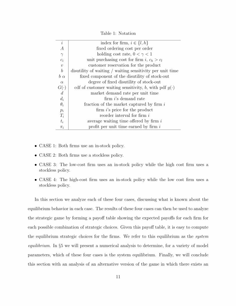
Table 1: Notation
i index for firm, i ∈ {l, h}A fixed ordering cost per orderγ holding cost rate, 0 < γ < 1ci unit purchasing cost for firm i, ch > cl
v customer reservation for the productb disutility of waiting / waiting sensitivity per unit time
b α fixed component of the disutility of stock-outα degree of fixed disutility of stock-out
G(·) cdf of customer waiting sensitivity, b, with pdf g(·)d market demand rate per unit timedi firm i’s demand rateθi fraction of the market captured by firm i
pi firm i’s price for the productTi reorder interval for firm i
ti average waiting time offered by firm i
πi profit per unit time earned by firm i
• CASE 1: Both firms use an in-stock policy.
• CASE 2: Both firms use a stockless policy.
• CASE 3: The low-cost firm uses an in-stock policy while the high cost firm uses astockless policy.
• CASE 4: The high-cost firm uses an in-stock policy while the low cost firm uses astockless policy.
In this section we analyze each of these four cases, discussing what is known about the
equilibrium behavior in each case. The results of these four cases can then be used to analyze
the strategic game by forming a payoff table showing the expected payoffs for each firm for
each possible combination of strategic choices. Given this payoff table, it is easy to compute
the equilibrium strategic choices for the firms. We refer to this equilibrium as the system
equilibrium. In §5 we will present a numerical analysis to determine, for a variety of model
parameters, which of these four cases is the system equilibrium. Finally, we will conclude
this section with an analysis of an alternative version of the game in which there exists an
11
incumbent firm and a potential new entrant to the market.
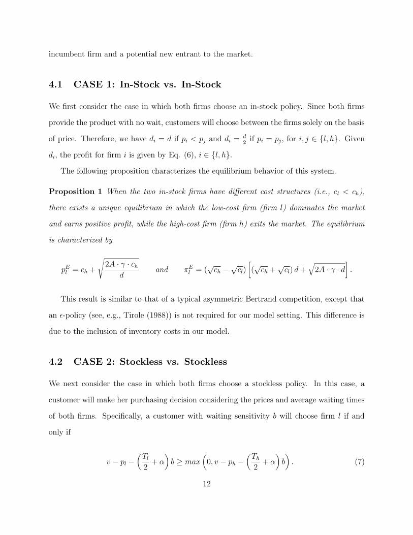
4.1 CASE 1: In-Stock vs. In-Stock
We first consider the case in which both firms choose an in-stock policy. Since both firms
provide the product with no wait, customers will choose between the firms solely on the basis
of price. Therefore, we have di = d if pi < pj and di = d2
if pi = pj, for i, j ∈ {l, h}. Given
di, the profit for firm i is given by Eq. (6), i ∈ {l, h}.
The following proposition characterizes the equilibrium behavior of this system.
Proposition 1 When the two in-stock firms have different cost structures (i.e., cl < ch),
there exists a unique equilibrium in which the low-cost firm (firm l) dominates the market
and earns positive profit, while the high-cost firm (firm h) exits the market. The equilibrium
is characterized by
pEl = ch +
√
2A · γ · ch
dand πE
l = (√
ch −√
cl)[
(√
ch +√
cl) d +√
2A · γ · d]
.
This result is similar to that of a typical asymmetric Bertrand competition, except that
an ε-policy (see, e.g., Tirole (1988)) is not required for our model setting. This difference is
due to the inclusion of inventory costs in our model.
4.2 CASE 2: Stockless vs. Stockless
We next consider the case in which both firms choose a stockless policy. In this case, a
customer will make her purchasing decision considering the prices and average waiting times
of both firms. Specifically, a customer with waiting sensitivity b will choose firm l if and
only if
v − pl −(
Tl
2+ α
)
b ≥ max
(
0, v − ph −(
Th
2+ α
)
b
)
. (7)
12
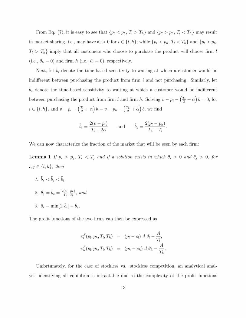
From Eq. (7), it is easy to see that {pl < ph, Tl > Th} and {pl > ph, Tl < Th} may result
in market sharing, i.e., may have θi > 0 for i ∈ {l, h}, while {pl < ph, Tl < Th} and {pl > ph,
Tl > Th} imply that all customers who choose to purchase the product will choose firm l
(i.e., θh = 0) and firm h (i.e., θl = 0), respectively.
Next, let b̃i denote the time-based sensitivity to waiting at which a customer would be
indifferent between purchasing the product from firm i and not purchasing. Similarly, let
b̃s denote the time-based sensitivity to waiting at which a customer would be indifferent
between purchasing the product from firm l and firm h. Solving v − pi −(
Ti
2+ α
)
b = 0, for
i ∈ {l, h}, and v − pl −(
Tl
2+ α
)
b = v − ph −(
Th
2+ α
)
b, we find
b̃i =2(v − pi)
Ti + 2αand b̃s =
2(pl − ph)
Th − Tl
.
We can now characterize the fraction of the market that will be seen by each firm:
Lemma 1 If pi > pj, Ti < Tj and if a solution exists in which θi > 0 and θj > 0, for
i, j ∈ {l, h}, then
1. b̃s < b̃j < b̃i,
2. θj = b̃s = 2(pl−ph)Th−Tl
, and
3. θi = min[1, b̃i] − b̃s.
The profit functions of the two firms can then be expressed as
πSl (pl, ph, Tl, Th) = (pl − cl) d θl −
A
Tl
,
πSh (pl, ph, Tl, Th) = (ph − ch) d θh −
A
Th
.
Unfortunately, for the case of stockless vs. stockless competition, an analytical anal-
ysis identifying all equilibria is intractable due to the complexity of the profit functions
13
and the interactions among the four decision variables. Thus, to investigate the equilibria
numerically, we first set up the profit maximization problem for the individual firm as a
nonlinear optimization problem using GAMS. The GAMS program adopts a systematical
and exhaustive search algorithm. We then use a standard iterative approach to determine
the equilibrium:
1. Given firm j’s decision variables, i.e., pj, Tj, firm i determines its optimal decision
variables, i.e., p∗i (pj, Tj), T ∗i (pj, Tj). In doing so, two options are considered:
• Firm i may choose to serve those customers who are more sensitive to waiting
time by choosing pi > pj, Ti < Tj.
• Firm i may choose to serve those customers who are less sensitive to waiting time
by choosing pi < pj, Ti > Tj.
2. Given firm i’s optimal decision variables, p∗i , T ∗
i , firm j determines its optimal decision
variables in a similar manner.
3. The program terminates when a given firm cannot deviate (or improve its profit) from
one iteration to the next.
For each set of problem parameters considered, we implemented this iterative approach
for a wide range of initial values for pj and Tj. Specifically, we considered 5 initial prices (i.e.,
ch+ 1−ch
6·n, where n = 1 . . . 5) and 5 initial reorder intervals (i.e., T ∗
h ·n, where n = 1 . . . 5 and
T ∗h is the optimal reorder interval for a monopoly firm following a stockless policy). In sum,
the GAMS program considers 25 initial starting points for each set of problem parameters.
After conducting a comprehensive numerical study in which we varied numerous model
parameters (refer to §5 for further details), we find that there exists only one type of equi-
librium for the case of stockless vs. stockless competition. Specifically, in all cases we find
that firm l will serve the market, while firm h will exit the market. This result suggests that
14
the main result of the typical asymmetric Bertrand competition model, in which the firms
compete only on price, also applies to the case in which two stockless firms compete on both
price and customer waiting time.
4.3 CASE 3: Low-cost Firm with In-stock Policy vs. High-cost
Firm with Stockless Policy
We next consider the case in which the two firms choose different inventory policies. We will
start by considering the case in which firm l chooses an in-stock policy and firm h chooses a
stockless policy. Analogous results, although not presented here, will apply for the reverse
case (CASE 4). All of the analytical results for CASE 4 can be derived by interchanging the
key subscripts (i.e., l and h) in the propositions in this section.
We first note that, for any set of prices and reorder intervals, there are three possible
outcomes: i) all customers prefer the high-cost stockless firm; ii) all customers prefer the
low-cost in-stock firm; or iii) the customers’ preferences are split between the two firms. We
will investigate the equilibrium behavior for each of these cases, starting with the case in
which the firms split the market.
4.3.1 High-cost and Low-cost Firm Split the Market
In this section we consider the case in which each firm captures some portion of the market.
We are interested in determining whether or not there exists an equilibrium in which both
firms will make positive profit (a necessary requirement for both firms to participate in the
market). If such an equilibrium exists, we then would like to determine the equilibrium
values of ph, Th and pl, which we denote by pEh , TE
h and pEl , respectively. Recall that the
in-stock firm, i.e., firm l, will always choose T El =
√
2Adlγcl
.
Since pi ≤ v for i ∈ {l, h}, a customer with waiting time sensitivity b will choose to
15
purchase the product from firm h if v − ph −(
Th
2+ α
)
b > v − pl. Thus, the fraction of the
market that will purchase from firm h, θh, can be written as
θh = Pr
{
b <2(pl − ph)
Th + 2α
}
= max
[
0, min
[
1,2(pl − ph)
Th + 2α
]]
. (8)
Since all customers will purchase the product (because pl < v), we have θl = 1 − θh.
We want to consider the case in which the firms split the market, i.e., 0 < θi < 1 for i ∈
{l, h}. From Eq. (8), this will hold only under the following condition: ph < pl < ph+α+ Th
2.
Therefore, we will start our analysis by considering the optimal policy for the high-cost firm
given pl, where pl satisfies ph < pl < ph + α + Th
2.
Let p∗h(pl) and T ∗h (pl) denote the optimal price and reorder interval for the high-cost firm
given the price, pl, offered by the low-cost firm. Similarly, we define θ∗h(pl) and πS∗
h (pl) to
be the optimal market share and profit for the high-cost firm given pl, respectively. The
following proposition presents our key results on the behavior of these functions.
Proposition 2 If ch +√
2Ad
< pl < ch +√
2Ad
+ 2α, then
i) p∗h(pl) =1
2(pl + ch), ii) T ∗
h (pl) =−4α
√A
2√
A −√
2d√
(ch − pl)2> 0,
iii) 0 < θ∗h(pl) < 1, iv) πS∗h (pl) > 0, and v)
dπS∗h
dpl
> 0.
We are interested in the profit earned by the low-cost firm given that the high-cost firm
uses the optimal parameters p∗h(pl) and T ∗
h (pl), as defined above. We use πIl (pl|p∗h, T ∗
h ) to
denote this profit function. We next demonstrate that this profit will be positive when
ch +√
2Ad
< pl < ch +√
2Ad
+ 2α.
Proposition 3 For pl satisfying ch +√
2Ad
< pl < ch +√
2Ad
+ 2α, πIl (pl|p∗h, T ∗
h ) > 0.
Together, Propositions 2 and 3 present conditions under which, acting optimally, the
16
high-cost firm will choose a price and reorder interval such that the two firms will split
the market (0 < θ∗h(pl) < 1) and both firms will earn positive profits (πS∗h (pl) > 0 and
πIl (pl|p∗h, T ∗
h ) > 0).
Finally, the following proposition demonstrates the conditions under which there will be
a unique equilibrium solution for this case.
Proposition 4 If ch +√
2Ad
< pl < ch +√
2Ad
+ 2α, when the low-cost firm uses an in-stock
policy and the high-cost firm uses a stockless policy, there exists a unique equilibrium.
Further context for the results of Propositions 2, 3, and 4 is provided in the next section.
4.3.2 Only One Firm Serves the Market
In the previous section, we considered the case in which the low-cost in-stock firm and the
high-cost stockless firm split the market. We next consider the two extreme cases: (1) only
the high-cost stockless firm serves the market and (2) only the low-cost in-stock firm serves
the market.
The first extreme case (all customers prefer the high-cost stockless firm) implies θh = 1,
which is equivalent to the condition pl ≥ ph + Th
2+ α. For this case, we can show that an
equilibrium does not exist.
Proposition 5 There is no equilibrium that satisfies i) the low-cost firm chooses an in-stock
policy, ii) the high-cost firm chooses a stockless policy, and iii) pl ≥ ph + Th
2+ α.
The second extreme case (all customers prefer the low-cost in-stock firm) implies θh =
0, which (since Th > 0) directly implies that pl ≤ ph. In the following proposition, we
characterize the equilibrium solution for this case.
17
Proposition 6 When i) the low-cost firm chooses an in-stock policy, ii) the high-cost firm
chooses a stockless policy, and iii) pl ≤ ph, there exists an equilibrium characterized by
pEl = ch +
√
2Ad
if ch +√
2Ad
< v,
pEl = v otherwise,
TEl =
√
2Adlγcl
.
To summarize, Propositions 2, 3, and 4 characterize an equilibrium in which two firms
will serve some fraction of the market and make positive profit, while Propositions 5 and 6
demonstrate that an equilibrium might occur at the extreme point in which only the low-cost
firm serves the market, but not at the other extreme in which only the high-cost firm serves
the market. The type of equilibrium is determined by the low-cost firm because the price
given in Proposition 6 does not allow the firm high-cost firm to take any fraction of the
market with positive profit. Specifically, we can determine the nature of the equilibrium for
CASE 3 as follows: Using Proposition 2, we can write the profit for the low cost firm as a
function of pl, given that ph and Th are chosen optimally. We can then find the value of pl
that maximizes this profit. If this value satisfies ch +√
2Ad
< pl < ch +√
2Ad
+ 2α, then both
firms stay in the market; otherwise, only the low cost firm serves the market. In other words,
for any set of problem parameters, we can determine whether the equilibrium for CASE 3
will satisfy the conditions of Propositions 2 - 4 or of Proposition 6.
4.4 An Incumbent-Entrant Game
So far in our analysis, we have assumed that each firm may choose either the in-stock policy
or the stockless policy. In this subsection, we consider an important alternative formulation
in which there exists in the market an incumbent firm, assumed to be the low-cost firm
(perhaps due to economies of scale or learning curve effects) which follows a traditional in-
18
stock policy. A new high-cost firm is considering entering the market and must make several
decisions: whether or not to enter the market, whether to use an in-stock or stockless policy,
and how to set the price and reorder interval.
We can easily use the analytical results obtained in this section to characterize the equi-
librium solution for this problem. From Proposition 1, we know that if the high-cost entrant
attempts to enter the market using an in-stock policy, he will be forced from the market by
the incumbent low-cost firm. Thus, any new entrant will choose a stockless policy and the
results of §4.3 (CASE 3) will apply. Finally, using the approach outlined above (in the final
paragraph of §4.3.2), we can easily determine the nature of the resulting equilibrium, i.e.,
we can determine whether or not the entrant will remain in the market.
5 Analysis of Firms’ Strategic Choices
In this section, we conduct a series of numerical analyses in order to better understand how
the two firms make their strategic choices, i.e., choose between the in-stock and stockless
policies, and how a variety of experimental parameters affect the profits of both firms.
The values of the experimental parameters used in the analysis are summarized as
follows: 1) fixed ordering cost per order (A ∈ {1, 3, 5}), 2) inventory holding cost rate
(γ ∈ {0.1, 0.2, 0.3}), 3) unit purchasing cost (ci ∈ {0.2, 0.3, 0.4}), 4) demand rate (d ∈
{100, 500, 1000}), and 5) degree of fixed disutility of stock-out (α ∈ {0.01, 0.2, 0.4, 0.6, 0.8}).
This parameter setting results in 405 (= 3 × 3 × 3 × 3 × 5) unique experimental problems.
5.1 Analysis of System Equilibrium
In this section, we present the results of our numerical study on the nature of the system
equilibrium, as defined in §4. As noted in §4, we find the system equilibrium by solving a
strategic game with a 2 × 2 payoff table.
19
We find that 303 out of 405 problems (74.8%) have a unique Nash equilibrium. Among
these, only one firm serves the market (refer to Proposition 6) in 87 instances (28.7%), while
the two firms split the market in the remaining 72.3% (216 out of 303) of these problems.
For the problems in which a single firm serves the market, the surviving firm is the low-cost
firm and the strategic choice is an in-stock policy. For the problems in which the two firms
split the market, we know from the analysis in Sections 4.1 and 4.2 that an equilibrium does
not exist in which both firms serve the market and use the same strategy, i.e., stockless vs.
stockless or in-stock vs. in-stock cannot be an equilibrium. Thus, in all of the problems
with a single equilibrium in which both firms serve the market, we find that CASE 3 is the
equilibrium, i.e., the low-cost firm chooses an in-stock policy and the high-cost firm chooses
a stockless policy. Intuitively, the high-cost firm chooses a stockless policy in an attempt to
reduce its costs to a competitive level.
In 102 out of 405 problems (25.2%), two Nash equilibria exist; in each, one firm chooses
an in-stock policy and the other firm chooses a stockless policy. Two equilibria will exist
when the profit earned by the low-cost firm in CASE 4 (low-cost firm is stockless, high-cost
firm is in-stock) are greater than those earned in CASE 1 (low-cost firm is in-stock, high-cost
firm is in-stock, and only the low cost firm survives in the market), i.e., when the benefits of
stockless operations (relative to using an in-stock policy) for the low-cost firm outweigh the
benefits of having a monopoly. In this case, in addition to having CASE 3 (low-cost firm is
in-stock, high-cost firm is stockless) as an equilibrium, CASE 4 (low-cost firm is stockless,
high-cost firm is in-stock) becomes an equilibrium. Intuitively, the low cost firm will prefer
CASE 4 to CASE 1 when the holding cost rate is high and the ordering cost is small (these
conditions make the stockless policy more attractive relative to the in-stock policy) and when
the demand rate is large (this condition enables a firm that splits the market to achieve some
of the economies of scale that would be enjoyed by a monopoly). We also find that the low
cost firm will prefer CASE 4 to CASE 1 when the degree of fixed disutility (α) is moderate.
20

0
0.05
0.1
0.15
0.2
0.25
0.3
0.35
0.4
0 0.2 0.4 0.6 0.8 1
Degree of Fixed Disutility
Diff
. in
Pri
ce
(a) Difference in Price (i.e., pl − ph)
0
0.2
0.4
0.6
0.8
1
1.2
0 0.2 0.4 0.6 0.8 1
Degree of Fixed Disutility
Pri
ce
Firm l Firm h
(b) Equilibrium Prices
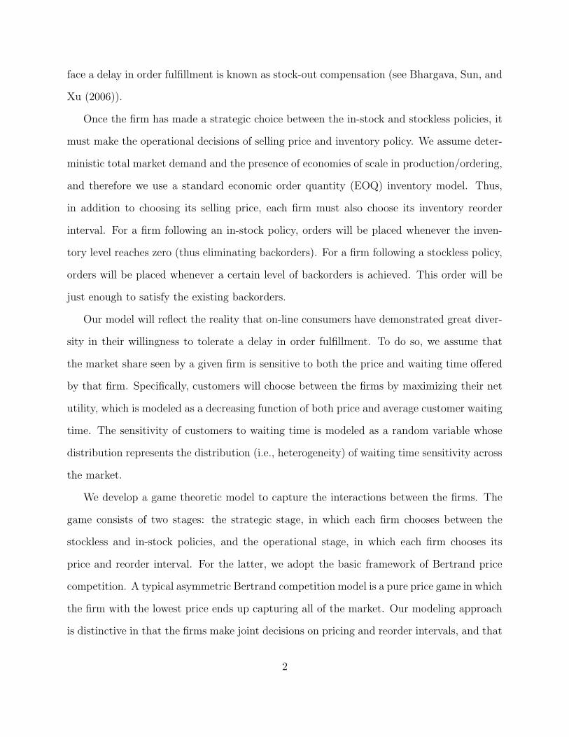
Figure 1: Effect of Degree of Fixed Disutility (A = 3, γ = 0.2, cl = 0.2, ch = 0.3, d = 500)
This behavior will be explained in detail later in this section. Thus, in summary, problems
with two equilibria are more likely when the holding cost rate is high, the ordering cost is
small, demand is large, and the degree of fixed disutility is moderate.
In the remainder of this section, we will focus our analysis on the case in which two firms
remain in the market, with the low-cost firm choosing an in-stock policy and the high-cost
firm choosing a stockless policy. As noted above, this is the most common outcome of our
model.
5.2 Favorable Conditions for Stockless Operations
We find that the firm that chooses an in-stock policy primarily dominates in the market. In
other words, at the Nash equilibria, the firm that chooses an in-stock policy maintains the
higher price and captures the greater market share. Thus, a firm which operates under a
stockless policy must practice stockout compensation, i.e., must offer a reduced price relative
to the competing in-stock firm. This result is demonstrated in Figure 1, which shows that
the price charged by the low-cost, in-stock firm is always higher than the price charged by
the high-cost, stockless firm. Thus, the stockless policy is in our model is best referred to
as stockless operations with stock-out compensation since stockless operations by itself, i.e.,
21

0
100
200
300
400
500
600
0 0.2 0.4 0.6 0.8 1
Degree of Fixed Disutility
Firm
l's
Pro
fitd=100 d=500 d=1000
(a) Firm l’s Equilibrium Profit
0
20
40
60
80
100
120
140
0 0.2 0.4 0.6 0.8 1
Degree of Fixed Disutility
Firm
h's
Pro
fit
d=100 d=500 d=1000
(b) Firm h’s Equilibrium Profit
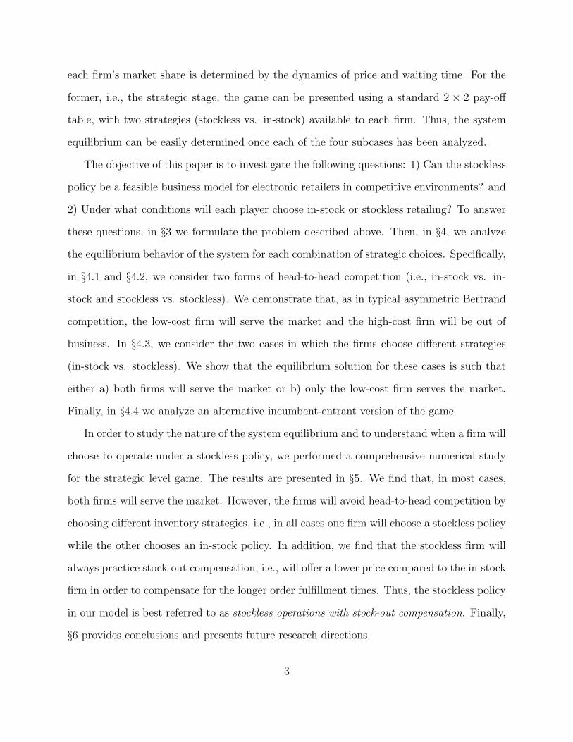
Figure 2: Equilibrium Profits (A = 3, γ = 0.2, cl = 0.2, ch = 0.3)
without stock-out compensation, is not a feasible strategy.
This observation leads to a key practical question: Under what environmental conditions
can a firm’s stockless policy be relatively profitable? From our comprehensive numerical
study, we found that a stockless policy can be favorable when there exist a high demand
rate, high inventory holding cost, low fixed ordering cost, medium degree of fixed disutility,
and a relatively small difference in purchasing costs between the two firms. In the following
discussion, we attempt to explain why these conditions are necessary for stockless operations
to be profitable by evaluating the impact of the key experimental parameters on both firm’s
optimal prices and profits.
Figure 1(b) illustrates the main effect of the degree of fixed disutility (α) on the optimal
prices. As the disutility increases, both firms’ optimal prices increase. In other words, as
α increases, customers prefer to purchase from the low-cost firm with the in-stock policy.
Under these circumstances, the low-cost firm would increase its price to maximize its profits,
which would lead the high-cost firm to increase its price, mimicking the low-cost firm’s high
price policy.
The interaction between the demand rate (d) and the degree of fixed disutility (α) can
be seen in Figure 2. As seen in the figure, the combination of a high rate of demand and
a high degree of fixed disutility creates favorable conditions for the low-cost firm. However,
22
00.05
0.10.15
0.20.25
0.30.35
0.40.45
0.5
0 0.2 0.4 0.6 0.8 1
Degree of Fixed DisutilityM
arke
t Sha
re
d=100 d=500 d=1000
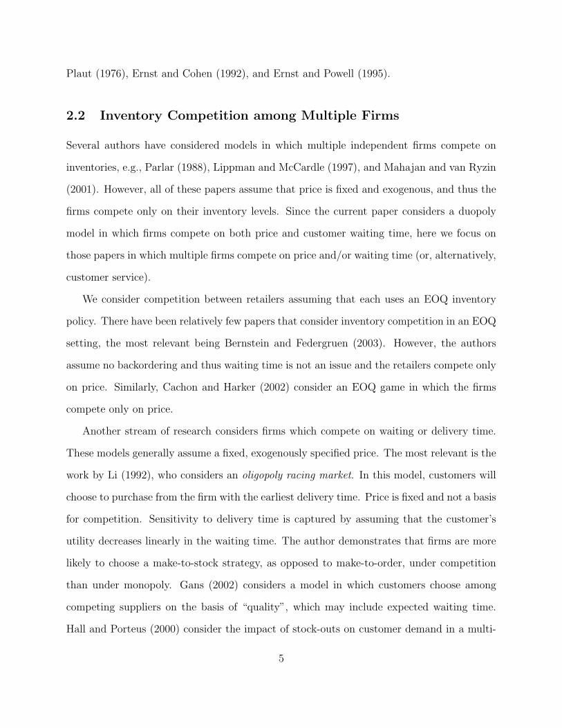
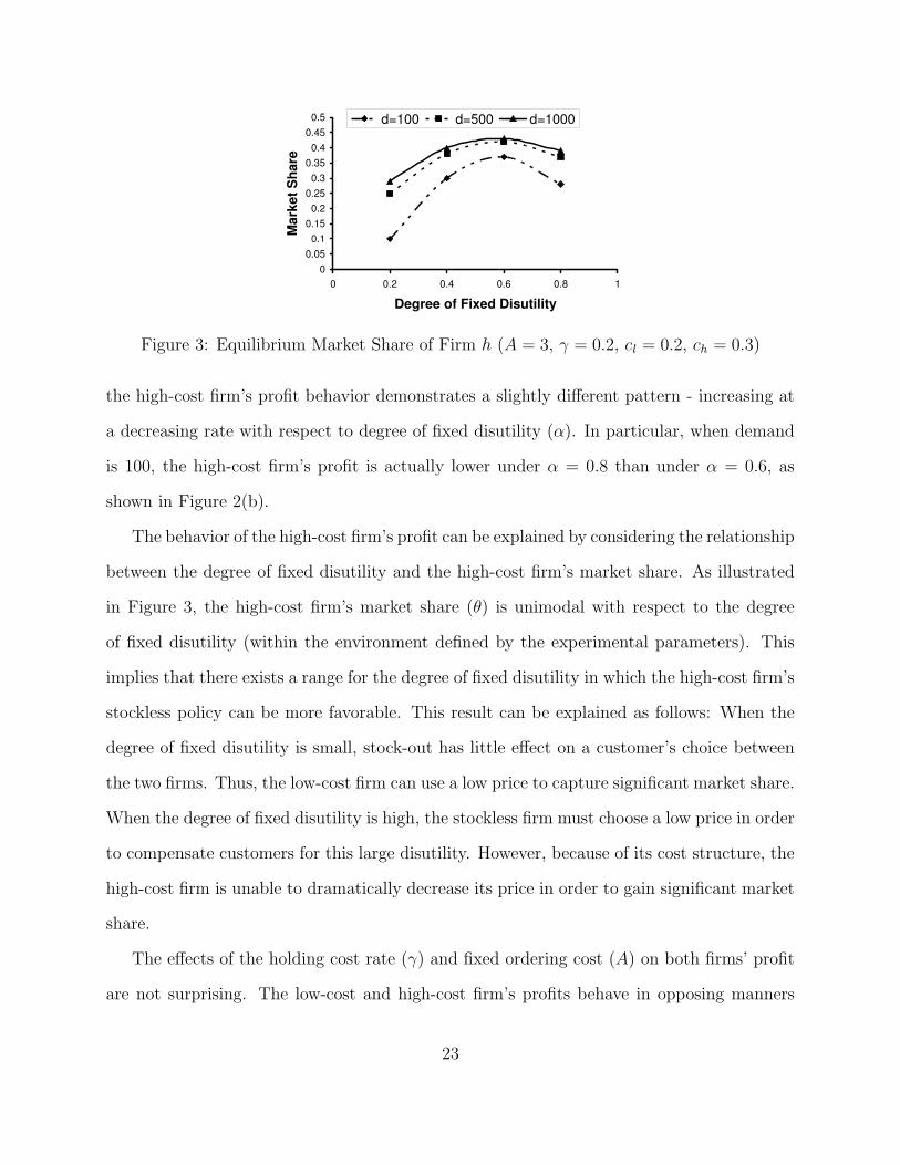
Figure 3: Equilibrium Market Share of Firm h (A = 3, γ = 0.2, cl = 0.2, ch = 0.3)
the high-cost firm’s profit behavior demonstrates a slightly different pattern - increasing at
a decreasing rate with respect to degree of fixed disutility (α). In particular, when demand
is 100, the high-cost firm’s profit is actually lower under α = 0.8 than under α = 0.6, as
shown in Figure 2(b).
The behavior of the high-cost firm’s profit can be explained by considering the relationship
between the degree of fixed disutility and the high-cost firm’s market share. As illustrated
in Figure 3, the high-cost firm’s market share (θ) is unimodal with respect to the degree
of fixed disutility (within the environment defined by the experimental parameters). This
implies that there exists a range for the degree of fixed disutility in which the high-cost firm’s
stockless policy can be more favorable. This result can be explained as follows: When the
degree of fixed disutility is small, stock-out has little effect on a customer’s choice between
the two firms. Thus, the low-cost firm can use a low price to capture significant market share.
When the degree of fixed disutility is high, the stockless firm must choose a low price in order
to compensate customers for this large disutility. However, because of its cost structure, the
high-cost firm is unable to dramatically decrease its price in order to gain significant market
share.
The effects of the holding cost rate (γ) and fixed ordering cost (A) on both firms’ profit
are not surprising. The low-cost and high-cost firm’s profits behave in opposing manners
23

with respect to inventory holding cost and ordering cost. Since the high-cost firm’s total
inventory cost is just the sum of the fixed ordering costs, its profit decreases as the fixed
ordering cost increases. Thus, a high ordering cost is in favor of the low-cost firm with in-
stock policy. In contrast, as the holding cost rate increases, the low-cost firm’s profit declines
and the high-cost firm’s profit increases. Because the high-cost firm does not hold inventory,
the increased holding cost rate only affects the low-cost firm’s profit. Therefore, a higher
rate of inventory holding cost favors the high-cost firm.
6 Concluding Remarks
In this paper we have considered a duopoly model in which two electronic retailers compete
to capture a larger market share using alternative pricing-inventory strategies (in-stock vs.
stockless). The objective of our analysis was to investigate whether the stockless policy can
be a viable online business model in the presence of competition. Based on the analytical
models developed in this paper, along with the corresponding computational study, we found
that, unlike the typical outcome of asymmetric Bertrand price competition in which one firm
is always driven out of competition, two retailers can coexist in the market by choosing a
policy (for example, a stockless policy) which differs from their competitor’s policy (for
example, an in-stock policy).
There are several significant contributions made in this paper. First, we show that the
stockless policy is a legitimate option for a firm which intends to avoid head-to-head com-
petition with the existing dominant player in the traditional market. In other words, it
is possible for a firm to establish a profitable business by creating virtual stores to attract
customers who may be less sensitive to waiting time for product delivery. Second, we demon-
strate that a stockless firm must offer a reduced price relative to the competing in-stock firm.
Thus, in practice, the stockless policy becomes stockless operations with stock-out compen-
24
sation. Third, we identify a set of conditions that may help stockless policies become more
profitable. These conditions include a high demand rate, a medium degree of fixed disutility,
a low ordering cost, a high inventory holding cost rate, and a purchasing cost comparable to
that of other retailers.
Finally, there are numerous ways in which this research can be extended and improved
upon. As discussed above, there are many reasons why a firm may choose to use a zero
(or very low) inventory policy. One important reason not captured in this paper is demand
uncertainty. It is well known that high demand uncertainty can lead to high inventory
requirements and significant inventory costs. Thus, a stockless operation, coupled with
stock-out compensation, may prove to be a profitable alternative for firms facing high demand
uncertainty. Further research in this direction would be an interesting extension of our work.
In addition, in this paper we assume that a firm must choose a single mode of competition
(either in-stock or stockless policy) since our objective was to provide clear comparisons
between the two policies under investigation. We have also used the Uniform distribution to
represent the customers’ heterogeneity in their sensitivity to waiting. Future research will
improve upon the present study by allowing the possibility that a firm can choose a policy
in between the extreme in-stock and stockless policies and by considering more general
probability distributions to represent the customers’ sensitivity to waiting.
References
Bernstein, F., and A. Federgruen (2003): “Pricing and Replenishment Strategies in aDistribution System with Competing Retailers,” Operations Research, 51, 409–426.
(2004): “A General Equilibrium Model for Industries with Price and Service Com-petition,” Operations Research, 52, 868–886.
Bhargava, H. K., D. Sun, and S. H. Xu (2006): “Stockout Compensation: Joint Inven-tory and Price Optimization in Electronic Retailing,” INFORMS Journal on Computing,18(2), 255–266.
25
Cachon, G. P., and P. T. Harker (2002): “Competition and Outsourcing with ScaleEconomies,” Management Science, 48, 1314–1333.
Caine, G. J., and R. H. Plaut (1976): “Optimal Inventory Policy when Stock-outs AlterDemand,” Naval Research Logistics Quarterly, 23, 1–13.
Chan, L. M. A., Z. J. M. Shen, D. Simchi-Levi, and J. Swann (2004): “Coordinationof Pricing and Inventory Decisions: A Survey and Classification,” in Handbook of Quan-titative Supply Chain Analysis: Modeling in the E-Business Era, ed. by D. Simchi-Levi,S. D. Wu, and Z. J. M. Shen, pp. 335–392. Kluwer Academic Publishers.
Cheung, K. L. (1998): “A Continuous Review Inventory Model with a Time Discount,”IIE Transactions, 30, 747–757.
Dana, J. D., and N. C. Petruzzi (2001): “The Newsvendor Model with EndogenousDemand,” Management Science, 47, 1488–1497.
Ernst, R., and M. A. Cohen (1992): “Coordination Alternatives in a Manufac-turer/Dealer Inventory System under Stochastic Demand,” Production and OperationsManagement, 1, 254–268.
Ernst, R., and S. G. Powell (1995): “Optimal Inventory Policies under Service-SensitiveDemand,” European Journal of Operational Research, 87, 316–327.
Gans, N. (2002): “Customer Loyalty and Supplier Quality Competition,” ManagementScience, 48, 207–221.
Hadley, G., and T. M. Whitin (1963): Analysis of Inventory Systems. Prentice HallInc., Englewood Cliffs, NJ.
Hall, J., and E. Porteus (2000): “Customer Service Competition in Capacitated Sys-tems,” Manufacturing & Service Operations Management, 2, 144–165.
Hassin, R. (1986): “Consumer Information in Markets with Random Product Quality: theCase of Queues and Balking,” Econometrica, 54(5), 1185–1196.
Karpinski, R. (1999): “The logistics of e-business? Web commerce demands new approachto inventory, shipping,” InternetWeek, http://internetweek.cmp.com/lead/lead052799.htm.
Kunreuther, H., and J. F. Richard (1971): “Optimal Pricing and Inventory Decisionsfor Non-Seasonal Items,” Econometrica, 39, 173–175.
Lederer, P. J., and L. Li (1997): “Pricing, Production, Scheduling, and Delivery-TimeCompetition,” Operations Research, 45(3), 407–420.
Li, L. (1992): “The Role of Inventory in Delivery-Time Competition,” Management Science,38, 182–197.
26

Li, L., and Y. S. Lee (1994): “Pricing and Delivery-Time Performance in a CompetitiveEnvironment,” Management Science, 40, 633–646.
Lippman, S. A., and K. F. McCardle (1997): “The Competitive Newsboy,” OperationsResearch, 45, 54–65.
Mahajan, S., and G. van Ryzin (2001): “Inventory Competition under Dynamic Con-sumer Choice,” Operations Research, 49, 646–657.
Majumder, P., and H. Groenevelt (2001): “Inventory Policy Implications of OnlinePurchase Behavior,” Working Paper, Simon School, University of Rochester, Rochester,NY.
Parlar, M. (1988): “Game Theoretic Analysis of the Substitutable Product InventoryProblem with Random Demand,” Naval Research Logistics, 35, 397–409.
Schwartz, B. L. (1970): “Optimal Inventory Policies in Perturbed Demand Models,”Management Science, 16, B509–B518.
Stidham, S. (1970): “On the Optimality of Single-Server Queuing Systems,” OperationsResearch, 18(4), 708–732.
Tirole, J. (1988): The Theory of Industrial Organization. MIT Press, Cambridge, MA.
Van Ackere, A., and P. Ninios (1993): “Simulation and Queueing Theory Applied toa Single-server Queue with Advertising and Balking,” The Journal of the OperationalResearch Society, 44(4), 407–414.
Vargas, M. T. (2000): “Decisions, Decisions, retail e-fulfillment,” Retail Industry,http://retailindustry.about.com/library/weekly/aa000718a.htm.
Whitin, T. M. (1955): “Inventory Control and Price Theory,” Management Science, 2,61–68.
Zipkin, P. H. (2000): Foundations of Inventory Management. McGraw Hill, Boston.
A Discussion of Disutility of Waiting
In this paper, we have considered a linear disutility of waiting, i.e., the disutility increases
linearly in t, the expected time to have an order filled. The idea that customers are delay-
sensitive and that the disutility of waiting is linear has been expressed by several other
authors. For example, Van Ackere and Ninios (1993), Hassin (1986), Li (1992), Li and Lee
27

(1994) and Stidham (1970) model the disutility of waiting in a similar, but more limited,
manner compared to our model. Specifically, they assume that all customers have the same
unit waiting cost, b, per unit time (i.e., customers are homogeneous and the disutility is
linear). In Lederer and Li (1997), the disutility of waiting is heterogeneous (as in our model).
However, a linear form is still assumed.
While most of the existing literature has assumed a linear form, it is quite possible that,
for some consumers, the disutility would follow a more complex form. For example, one
can imagine situations in which the disutility would be increasing and convex, reflecting the
fact that consumers will tolerate small waits, but become increasingly distressed by long
waits. Unfortunately, we have found that for even quite simple non-linear convex disutility
functions, our analytical model becomes intractable. Here we briefly demonstrate the main
difficulty in the analysis. Let g(t) be a general function of t (the expected waiting time) so
that the disutility of waiting for a customer with waiting sensitivity b is b(g(t)+α). Following
the procedures described in the paper, we have
θh = Pr
{
b <pl − ph
g(t) + α
}
= max
[
0, min
[
1,pl − ph
g(t) + α
]]
.
To analyze CASE 3 (low-cost firm with in-stock policy vs. high-cost firm with stockless
policy), we follow the procedures described in the proof of Proposition 2. Specifically, it is
easy to see that the condition∂πS
h
∂ph
= 0 is independent of Th. Thus, the optimal ph can be
set independently of Th. Solving∂πS
h
∂ph
= 0, we obtain p∗h(pl) = 12(pl + ch).
We next consider the first order conditions for Th. Using the fact that p∗h(pl) = 1
2(pl + ch)
for any Th, we have
∂πSh
∂Th
= −(pl − ch)2d
4
g′(
Th
2
)
(
g(
Th
2
)
+ α)2 +
A
T 2h
= 0
28
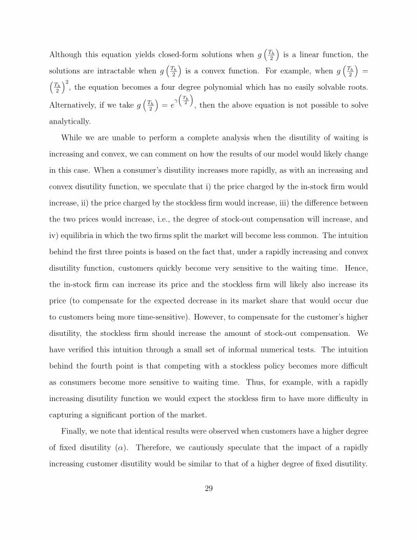
Although this equation yields closed-form solutions when g(
Th
2
)
is a linear function, the
solutions are intractable when g(
Th
2
)
is a convex function. For example, when g(
Th
2
)
=(
Th
2
)2, the equation becomes a four degree polynomial which has no easily solvable roots.
Alternatively, if we take g(
Th
2
)
= eγ
(
Th
2
)
, then the above equation is not possible to solve
analytically.
While we are unable to perform a complete analysis when the disutility of waiting is
increasing and convex, we can comment on how the results of our model would likely change
in this case. When a consumer’s disutility increases more rapidly, as with an increasing and
convex disutility function, we speculate that i) the price charged by the in-stock firm would
increase, ii) the price charged by the stockless firm would increase, iii) the difference between
the two prices would increase, i.e., the degree of stock-out compensation will increase, and
iv) equilibria in which the two firms split the market will become less common. The intuition
behind the first three points is based on the fact that, under a rapidly increasing and convex
disutility function, customers quickly become very sensitive to the waiting time. Hence,
the in-stock firm can increase its price and the stockless firm will likely also increase its
price (to compensate for the expected decrease in its market share that would occur due
to customers being more time-sensitive). However, to compensate for the customer’s higher
disutility, the stockless firm should increase the amount of stock-out compensation. We
have verified this intuition through a small set of informal numerical tests. The intuition
behind the fourth point is that competing with a stockless policy becomes more difficult
as consumers become more sensitive to waiting time. Thus, for example, with a rapidly
increasing disutility function we would expect the stockless firm to have more difficulty in
capturing a significant portion of the market.
Finally, we note that identical results were observed when customers have a higher degree
of fixed disutility (α). Therefore, we cautiously speculate that the impact of a rapidly
increasing customer disutility would be similar to that of a higher degree of fixed disutility.
29

To summarize, while the main findings of this paper are derived assuming a linear disu-
tility of waiting, we believe that our main result, i.e., that using a stockless operation with
stock-out compensation can be a profitable alternative in a competitive market, will still
hold.
B Technical Details & Proofs
Proof of Proposition 1. Let πI,1i and π
I,2i be firm i’s profit with market domination and
market sharing. First, note that
πI,1l (pi) − π
I,1h (pi) = (ch − cl)d +
√
2A · γ · d · (√ch −√
cl) > 0,
πI,2l (pi) − π
I,2h (pi) = (ch − cl)
d
2+√
A · γ · d · (√ch −√
cl) > 0,
and that all four of these profit functions are strictly increasing-linear functions of pi. There-
fore, the rest of the proof follows standard proof procedures of Bertrand competition (see,
e.g., Tirole (1988)). Here we demonstrate why the equilibrium price does not cause any de-
viation. Note that at the equilibrium price, firm h’s profit is zero with market domination.
Since this price is also acceptable to firm l, firm l serves the market. Now, firm h needs to
exit the market because it will have negative profit if it shares the market at the equilibrium
price.
Proof of Lemma 1. Let NSi(bk) be net surplus of a customer with waiting sensitivity
bk from purchasing a product from firm i (i.e., v−pi−(
Ti
2+ α
)
bk). First, note that NSi(bk) is
a linear-decreasing function of bk. Therefore, combining the precondition ({pl > ph, Tl < Th}
or {pl < ph, Tl > Th}) and the linearity implies that there exists at most one intersection
(i.e., b̃s) on bk. Next, the precondition of strictly positive market share implies b̃s < 1, which
implies that NSl(bk) and NSh(bk) intersect where bk < 1.
30
Now consider the case where pl > ph and Tl < Th. Under this case, we see that NSh(bk) >
NSl(bk) where bk < b̃s and NSh(bk) < NSl(bk) where bk > b̃s. Therefore, it is easy to see
that 1) b̃s < b̃h < b̃l, 2) customers whose waiting sensitivity is less than b̃s prefer firm h,
and 3) the other customers whose waiting sensitivity is greater than b̃s AND net surplus
is greater than 0 prefer firm l. The proof of the other case {pl < ph, Tl > Th} is exactly
identical to this procedure.
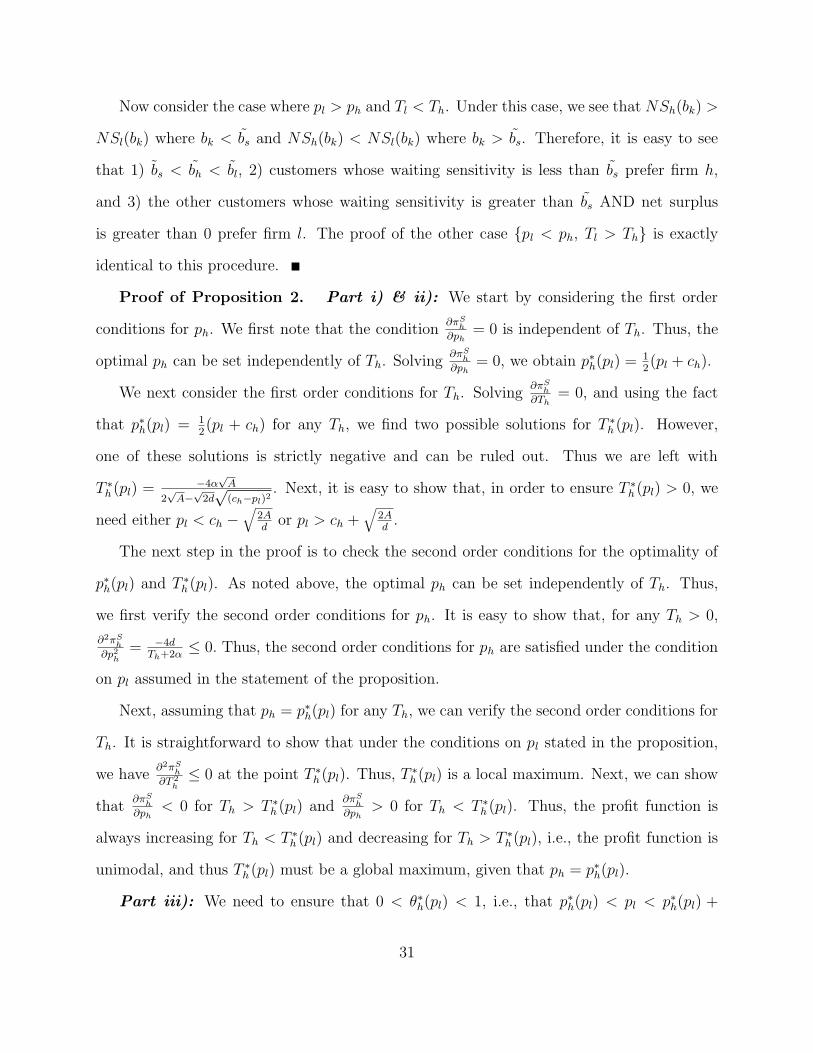
Proof of Proposition 2. Part i) & ii): We start by considering the first order
conditions for ph. We first note that the condition∂πS
h
∂ph
= 0 is independent of Th. Thus, the
optimal ph can be set independently of Th. Solving∂πS
h
∂ph
= 0, we obtain p∗h(pl) = 12(pl + ch).
We next consider the first order conditions for Th. Solving∂πS
h
∂Th
= 0, and using the fact
that p∗h(pl) = 12(pl + ch) for any Th, we find two possible solutions for T ∗
h (pl). However,
one of these solutions is strictly negative and can be ruled out. Thus we are left with
T ∗h (pl) = −4α
√A
2√
A−√
2d√
(ch−pl)2. Next, it is easy to show that, in order to ensure T ∗
h (pl) > 0, we
need either pl < ch −√
2Ad
or pl > ch +√
2Ad
.
The next step in the proof is to check the second order conditions for the optimality of
p∗h(pl) and T ∗h (pl). As noted above, the optimal ph can be set independently of Th. Thus,
we first verify the second order conditions for ph. It is easy to show that, for any Th > 0,
∂2πS
h
∂p2
h
= −4dTh+2α
≤ 0. Thus, the second order conditions for ph are satisfied under the condition
on pl assumed in the statement of the proposition.
Next, assuming that ph = p∗h(pl) for any Th, we can verify the second order conditions for
Th. It is straightforward to show that under the conditions on pl stated in the proposition,
we have∂2πS
h
∂T 2
h
≤ 0 at the point T ∗h (pl). Thus, T ∗
h (pl) is a local maximum. Next, we can show
that∂πS
h
∂ph
< 0 for Th > T ∗h (pl) and
∂πS
h
∂ph
> 0 for Th < T ∗h (pl). Thus, the profit function is
always increasing for Th < T ∗h (pl) and decreasing for Th > T ∗
h (pl), i.e., the profit function is
unimodal, and thus T ∗h (pl) must be a global maximum, given that ph = p∗h(pl).
Part iii): We need to ensure that 0 < θ∗h(pl) < 1, i.e., that p∗h(pl) < pl < p∗h(pl) +
31

α +T ∗
h(pl)
2. To ensure that pl > p∗h(pl) = 1
2(pl + ch), we need pl > ch. To ensure that
pl < p∗h(pl) + α +T ∗
h(pl)
2= 1
2(pl + ch) + α +
T ∗
h(pl)
2, we need pl < ch + T ∗
h (pl) + 2α. If
we plug in T ∗h (pl), using the fact that pl > ch, we find that pl < p∗h(pl) + α +
T ∗
h(pl)
2will
hold only if pl < ch +√
2Ad
+ 2α. Thus, we have shown that 0 < θ∗h(pl) < 1 will hold if
ch < pl < ch +√
2Ad
+ 2α.
The conditions required for T ∗h (pl) > 0 are pl < ch −
√
2Ad
or pl > ch +√
2Ad
, while the
conditions required for 0 < θ∗h(pl) < 1 are ch < pl < ch +√
2Ad
+ 2α. Combining these two
sets of conditions, we obtain ch +√
2Ad
< pl < ch +√
2Ad
+ 2α, as assumed in the statement
of the proposition.
Part iv): We next show that, under the condition on pl in the statement of the propo-
sition, πS∗h (pl) > 0. We can write πS∗
h (pl) = (p∗h(pl)− ch)d θ∗h(pl)− AT ∗
h(pl)
= d2
(pl−ch)2
T ∗
h(pl)+2α
− AT ∗
h(pl)
,
where the last step follows from the fact that pl − p∗h(pl) = 12(pl − ch). The condition
πS∗h (pl) > 0 can now be rewritten as
T ∗
h(pl)
T ∗
h(pl)+2α
> 2Ad(pl−ch)2
.
Plugging in for T ∗h (pl) and simplifying, we obtain
T ∗
h(pl)
T ∗
h(pl)+2α
=√
2Ad
1√(ch−pl)2
. Thus, the
condition πS∗h (pl) > 0 requires that
√
2Ad
1√(ch−pl)2
> 2Ad(pl−ch)2
. Simplifying and using the fact
that pl > ch, we obtain pl > ch +√
2Ad
. Thus, under the condition on pl in the proposition,
πS∗h (pl) > 0.
Part v): We next show that πS∗h (pl) is an increasing function of pl. Taking the derivative
with respect to pl, we have:
∂πS∗h
∂pl
=d(pl − ch)
T ∗h (pl) + 2α
+
(
A
T ∗2h (pl)
− d
2
(pl − ch)2
(T ∗h (pl) + 2α)2
)
dT ∗h (pl)
dpl
.
Using the proof of Part iv), we can show that(
AT ∗2
h(pl)
− d2
(pl−ch)2
(T ∗
h(pl)+2α)2
)
= 0. Thus, pl > ch
implies that∂πS∗
h
∂pl
> 0.
Proof of Proposition 3. To prove this proposition, we proceed in two steps: i) we
show that πIl (pl|p∗h, T ∗
h ) = 0 when pl = ch +√
2Ad
and ii) we prove that∂πI
l(pl|p∗h,T ∗
h)
∂pl
> 0 if
32

ch +√
2Ad
< pl < ch +√
2Ad
+ 2α. Together, these two results ensure that πIl (pl|p∗h, T ∗
h ) > 0
for pl satisfying ch +√
2Ad
< pl < ch +√
2Ad
+ 2α.
To prove Part i), we first write πIl (pl|p∗h, T ∗
h ) = (pl−cl)d(1−θ∗h(pl))−√
2Aγcld(1 − θ∗h(pl)),
where θ∗h(pl) =2(pl−p∗
h)
T ∗
h+2α
implies that 1 − θ∗h(pl) = 12α
(
1 −√
2Ad
1pl−ch
)
. Next, note that pl =
ch +√
2Ad
implies that 1pl−ch
=√
d2A
. Thus, when pl = ch +√
2Ad
, we have 1 − θ∗h(pl) = 0.
Therefore, when pl = ch +√
2Ad
, we have πIl (pl|p∗h, T ∗
h ) = 0.
Next, to prove Part ii), we plug 1 − θ∗h(pl) into πIl (pl|p∗h, T ∗
h ), take the derivative with
respect to pl, and simplify to get∂πI
l(pl|p∗h,T ∗
h)
∂pl
= d2α
(
1 −√
2Ad
1pl−ch
(
1 − pl−cl
pl−ch
))
. Finally, using
the facts that pl > ch and ch > cl, we know that 1pl−ch
> 0 and (1 − pl−cl
pl−ch
) < 0. Therefore,
∂πI
l(pl|p∗h,T ∗
h)
∂pl
> d2α
> 0, which completes the proof.
Proof of Proposition 4. We show that πIl (pl|ph, Th) is a unimodal function of pl,
where πIl (pl|ph, Th) = (pl − cl)d(1 − θh(pl)) −
√
2Aγcld(1 − θh(pl)), where θh(pl) = 2(pl−ph)Th+2α
.
We take the first derivative, set it equal to 0, and rewrite the first order condition as
d
(
1 − 2(pl − ph)
Th + 2α
)
+ (pl − cl) · d(
− 2
Th + 2α
)
= − 2Aγcld
(Th + 2α)
√
(
1 − 2(pl−ph)Th+2α
)
. (9)
The LHS of Eq. (9) is a decreasing linear function of pl, while the RHS is a decreasing
concave function. We evaluate two functions at pl = 0, and see that LHS|pl=0 > 0 and
RHS|pl=0 < 0. Combining these two observations implies that Eq. (9) has at most two real
solutions.
When there exists no solution or two identical solutions, it is easy to see that∂πI
l(pl|ph,Th)
∂pl
≥
0, which implies that πIl (pl|ph, Th) is a strictly increasing function. Now, consider the case
in which there are two different real solutions. We note that∂πI
l(pl|ph,Th)
∂pl
|pl=0 > 0 and
∂πI
l(pl|ph,Th)
∂pl
|pl=pU
l
= −d(Th+2α+2(ph−cl)Th+2α
< 0, where pUl =
(
ph + Th
2+ α
)
is an upper bound
on pl derived from 2(pl−ph)Th+2α
≤ 1. This implies that pUl is located between two stationary
points. Therefore, πIl (pl|ph, Th) is a unimodal function of pl in [0, pU
l ]. This completes the
33
proof.
Proof of Proposition 5. We prove this result by contradiction. Suppose that there
is an equilibrium that satisfies pEl ≥ pE
h +T E
h
2+ α (by implication, πI
l = 0), πSh > 0, and
the other conditions of Proposition 5. Let pL,Ml be the lower bound of firm l’s price under a
monopolistic setting with an in-stock policy (i.e., πI,Ml (pL,M
l ) = 0).
First, consider pEh > p
L,Ml . For this case, we construct a pricing policy that generates
positive profit for firm l. To this end, note that firm l can set pl = pEh and make positive
profit, since all customers prefer firm l (i.e., b̃s = 0 & πI,Ml (pL,M
l + ε) > 0).
Second, consider the other case in which pEh ≤ p
L,Ml , and suppose that there exists an
equilibrium. We show that firm h is unable to generate positive profit. To this end, we solve
max πSh (ph, Th) = (ph − ch) · d · max
[
2(1 − ph)
Th + 2α, 1
]
− A
Th
s.t. ph ≤ pL,Ml = cl +
√
2Aγcl
d,
ph +Th
2+ α ≤ pL
l = ch +
√
2A
d.
The second constraint is derived from the fact that if firm h sets pEh +
T E
h
2+ α > pL
l , then
firm l would deviate by setting pl =(
pEh +
T E
h
2+ α
)
− ε and have positive profit (refer to
Propositions 2 and 3). First, note that the second constraint implies that max[
2(1−ph)Th+2α
, 1]
= 1.
Hence, πSh (ph, Th) becomes (ph − ch) · d − A
Th
. In addition, we see that the second constraint
is binding, i.e., ph = ch +√
2Ad−(
Th
2+ α
)
. Now, we rewrite the problem as
max πSh (ph, Th) =
√
2A
d−(
Th
2+ α
)
d − A
Th
s.t. 2
ch +
√
2A
d−
cl +
√
2Aγcl
d
− α
ph ≤ Th.
Solving for the optimal solutions, the unconstrained problem has two stationary points, i.e.,
34

T ∗i =
√
2Ad
or T ∗i = −
√
2Ad
. It is easy to see that T ∗i =
√
2Ad
is a global maximum. By
plugging into the profit function and simplifying, we have πSh (ph, Th) = −d · α. Therefore,
firm h cannot make positive profit in this range. This contradicts the equilibrium assumption
and completes the proof.
Proof of Proposition 6. Note that the equilibrium should satisfy pEl ≤ pE
h (by
implication, πSh = 0 & πI
l > 0). Next, let pLl and pU
l be the two bounds of Proposition 2,
i.e., pLl = ch +
√
2Ad
and pUl = ch +
√
2Ad
+ 2α. Since pLl < pU
l , we consider three scenarios:
Scenario 1: pUl ≤ pE
l : Note that there is no equilibrium that satisfies the preconditions of
Proposition 6 in this region, because firm h can reduce ph sufficiently so that it can dominate
the market.
Scenario 2: pLl < pE
l < pUl : There exists a unique solution so that two firms share the market
(refer to Proof of Proposition 2), but note that the solution does not satisfy pEl ≤ pE
h .
Scenario 3: pEl ≤ pL
l : Suppose that firm l sets pl = pLl . Then, firm h can consider two
strategies: dominating or sharing the market. Since dominating the market is not feasible
(see Proof of Proposition 5), we only need to consider sharing the market. We demonstrate
that firm h cannot make positive profit with this strategy. To this end, we solve
max πSh (ph, Th|pL
l ) = (ph − ch) · d · 2(pLl − ph)
Th + 2α− A
Th
s.t.2(pL
l − ph)
Th + 2α≤ 1,
where pLl = ch +
√
2Ad
. By taking the first derivative with respect to ph and setting it
equal to 0, we have p∗h =pL
l+ch
2. Simplifying the profit function with p∗
h and pLl , we have
πSh (Th|p∗h, pL
l ) = − 2AαTh(Th+2α)
, which implies that firm h is unable to make positive profit.
35