Why do tornados and hail storms rest on weekends?

ABSTRACT:

Daniel Rosenfeld and Thomas L. Bell Submitted to J. Geophys. Res.-Atmos.

When anthropogenic aerosols over the eastern USA during summertime are at their weekly mid-week peak, tornado and hail storm activity there is also near its weekly maximum. The weekly cycle in storm activity is statistically significant and unlikely to be due to natural variability. The pattern of variability supports the hypothesis that air pollution aerosols invigorate deep convective clouds in a moist, unstable atmosphere, to the extent of inducing production of large hailstones and tornados. This is caused by the effect of aerosols on cloud-drop nucleation, making cloud drops smaller, delaying precipitation-forming processes and their evaporation, and hence affecting cloud dynamics.

POPULAR SUMMARY: Human production of atmospheric pollution changes with the day of the week. In particular, production of particulate pollution (aerosols) in the U.S. is largest during the middle of the workweek and at a minimum on Sundays. Previous research on weather over the southeast U.S. during the summer months has shown that storms, on average, grow larger during the middle of the week, produce more clouds and rain, and are accompanied by more lightning activity. This behavior can be explained by the effect aerosols have on cloud formation: more aerosols provide more nuclei around which cloud droplets form, resulting in smaller cloud water droplets. Smaller droplets are lighter and, instead of falling from the cloud as rain, rise to greater heights where they freeze, releasing more heat that drives the cloud to even higher altitudes than they would normally reach. This has been verified by the Tropical Rainfall Measuring Mission (TRMM) satellite.

This theory predicts that storms formed in polluted air have stronger updrafts and generate more ice aloft. Such conditions favor formation of large hail stones. The invigorated storms generate tornados more readily. This paper examines data collected by the Storm Prediction Center of the National Weather Service to see if there are indeed more reported tornados and more hail storms in the middle of the week. Just as the theory of aerosol effects on storms predicts, we find that there are more summertime tornados and hail storms over the southeast U.S. during the middle of the week than on weekends. The theory also predicts that there should be less of an aerosol effect on storm behavior in the western half of the U.S. and during non-summer months, and our analysis of the data confirms this, too. The average aerosol concentrations in the atmosphere vary with the day of the week by only about 10%, and tornado and hail-storm frequencies vary only by about 10%. But what is the background level of aerosol pollution doing to our weather? The amounts and kinds of aerosol pollution have steadily changed over the past century. This research raises the possibility that we may be experiencing different levels of severe storm activity in recent decades compared with pre-industrial times because of aerosol pollution.

Author Information: Thomas L. Bell, Code 613.2 (Emeritus Scientist) NASAlGSFC Email: Thomas.L.Bell@nasa.gov

https://ntrs.nasa.gov/search.jsp?R=20110015368 2020-03-29T15:16:02+00:00Z

Why do tornados and hail storms rest on weekends?

Daniel Rosenfeld I * and Thomas L. Be1l2

ABSTRACT

This study shows for the first time statistical evidence that when anthropogenic aerosols

over the eastern USA during summertime are at their weekly mid-week peak, tornado and

hail storm activity there is also near its weekly maximum. The weekly cycle in

summertime storm activity for 1995-2009 was found to be statistically significant and

unlikely to be due to natural variability. It correlates well with the weekly cycle of other

previously observed measures of storm activity. The pattern of variability supports the

hypothesis that air pollution aerosols invigorate deep convective clouds in a moist,

unstable atmosphere, to the extent of inducing production of large hailstones and

tornados. This is caused by the effect of aerosols on cloud-drop nucleation, making cloud

drops smaller and hydrometeors larger. According to simulations the larger ice

hydrometeors contribute to more hail. The reduced evaporation from the larger

hydrometeors produces weaker cold pools. Simulations showed that too cold and fast

expanding pools inhibit the formation of tornados. The statistical observations suggest

that this might be the mechanism by which the weekly modulation in pollution aerosols is

causing the weekly cycle in severe convective storms during summer over the eastern

USA.

1 The Hebrew University of Jerusalem, Institute of Earth Sciences, Jerusalem 91904, Israel. 2 NASA/GSFC, Climate and Radiation Branch, Greenbelt, MD 20771, USA. *To whom correspondence should be addressed. E-mail: daniel.rosenfeld@huji.ac.il

2

1. Introduction

This study puts to a statistical test the hypothesis that air pollution increases the chance of

severe convective storms. The motivation for posing this question is based on physical

considerations that are described in Section 1.2 of the Introduction. These considerations

have already been partially supported by the observations of a weekly cycle in rainfall,

storm heights, and large-scale vertical winds, made by Bell et al [2008]. We believe this

hypothesis does two things: 1) it provides a framework for understanding the

observations originally reported by Bell et at. [2008]; and 2) it has been a very successful

tool for predicting weekly cycles in other meteorological quantities, some of which have

been reported elsewhere [e.g., lightning activity [Bell et al, 2009a], and fractional cloud

cover and cloud-top temperatures [mentioned in Bell et al, 2009b)], and some of which

(weekly cycles in hailstorm and tornado activity) are reported here.

We believe that a strong observational case is made in this paper for the existence of

a weekly cycle in hailstorm and tornado activity over the eastern U.S. during the summer.

We would not have looked for such evidence had we not had the physical theory we

present below to guide us. Nevertheless, we should emphasize that the observations we

report here only show a correlation in hailstorm and tornado activity with the well­

established weekly cycle in pollution over the same area, and correlations do not prove

causality. These observations provide the impetus for more detailed observational studies

and advances in modeling of the effects of aerosols on storm development that will be

capable of establishing the causal connection, a connection we can only present as a

hypothesis here.

3

1.1 The weekly cycle in rain intensity and lightning activity

The weekly cycle of working weekdays and resting weekends is associated with

weekly-varying levels of particulate air pollution [e.g., Bell et al., 2008]. This cycle has

been shown to be associated with weekly cycles of midweek rainfall amounts, stonn

heights [Bell et aI., 2008; Bell et al. 2009b], and lightning activity [Bell et al., 2009a] in

the wann and moist climate of summer months in the southeast USA. It was

hypothesized that this is caused by mid-week enhanced particulate air pollution

invigorating convective storms, as will be described in Section 1.2. Theoretical

considerations and cloud simulations, described in Section 1.3, support this hypothesis.

1.2 The physical basis for aerosols invigorating convective clouds

Particulate air pollution can invigorate convective storms whose cloud bases are

warm enough that the cloudy air has to rise several km before reaching the freezing level.

In clouds forming in pollution-free air, rain can develop and precipitate from the lower

parts of the cloud without freezing. This early rain can be inhibited by the pollution

aerosol particles that act as cloud drop condensation nuclei (CCN) and nucleate greater

concentrations of smaller cloud drops that are slower to coalesce into rain drops [Gunn

and Phillips, 1957]. In clouds with wann cloud-base temperatures the freezing level is

several km above cloud base, so that rain can develop and fall from the rising air in the

cloud. Because the effect of aerosols is to suppress coalescence, rain is delayed and a

larger fraction of the cloud water ascends above the O°C isotherm level, where it is

accreted on ice precipitation particles that fall and melt at lower levels [MaUnie and

Pantikis, 1995; Andreae et aI., 2004]. The additional release oflatent heat of freezing

4

aloft and reabsorbed heat at lower levels by the melting ice implies greater upward heat

transport for the same amount of surface precipitation in the more polluted atmosphere.

In addition, greater evaporative cooling of the cloud water in the downdrafts transfers

even more heat downward [Lee et ai., 2010]. This means that more instability is

consumed for the same amount of rainfall. The inevitable outcome is invigoration of the

convective clouds [Rosenfeid et ai., 2008]. Cloud simulations have supported this

hypothesis by showing that updrafts increase in warm-base clouds (- 20°C) with added

aerosols that suppress the warm-rain processes [Khain et ai., 2004, 2005, 2008; Khain

and Lynn, 2009; Wang, 2005; Tao et al., 2007; Lee et ai., 2008a; van den Heever et ai.

2006; van den Heever and Cotton 2007; Ntelekos et ai. 2009]. According to these

simulations, invigoration was not necessarily associated with added rainfall amounts.

Enhanced rainfall was simulated only in warm, moist, unstable and low shear

environments [Khain et ai., 2008; Lee et ai., 2008b; Fan et al., 2007 and 2009]. The

stronger updrafts and downdrafts resulted in more coherent organization of the simulated

convection that feeds back into the intensity of the storms [Nteiekos et ai. 2009; Lee et

ai., 2010]. The invigoration was supported also by observations of more polluted

convective clouds growing taller [Koren et ai., 2005, 2008 and 2010].

1.2 The physical basis for aerosols enhancing lightning, hail and tornadoes

The invigorated updrafts with added supercooled water and ice hydrometeors

provide the conditions for enhanced cloud electrification [Molinie and Pontikis, 1995;

Williams et ai., 2002; Andreae et ai., 2004]. However, the observational evidence was

questioned due to the difficulty in separating the roles of meteorology and aerosols

[Lyons et ai., 1998; Williams and Stanfill, 2002; Williams et ai., 2002; Williams, 2005].

5

Critical supporting observational evidence for the validity of the invigoration hypothesis

was obtained very recently, where volcanic aerosols, whose variability was completely

independent of meteorology, were observed to invigorate deep convective clouds over the

northwest subtropical Pacific Ocean and more than double the lightning activity [Yuan et

ai., 2011; Langenberg, 2011].

The greater amount of supercooled cloud water in polluted situations means greater

growth rate of ice hydrometeors. The stronger updrafts mean that larger hail stones can

be suspended in the cloud before falling to the ground. Therefore, it is reasonable to

expect that clouds in more polluted air would produce larger hail stones. This is

supported by some observations [Andreae et ai., 2004; Wang et ai., 2009] and

simulations [Storer et ai., 2010; Khain et ai., 2011].

The dynamics of convective storms respond to the initial changes in precipitation by

changes in the downdrafts and their evaporative cooling, which feed the cold pools and

their gust fronts. Early simulations [Gilmore et ai., 2004; van den Reever and Cotton,

2004] showed that storm dynamics was very sensitive to changes in hydrometeor size,

such that smaller hydrometeors created larger cold pools and stronger gust fronts that fed

back to the storm dynamics. Colder downdrafts would produce a faster moving gust front

that would tend to cause faster propagation of the squall line. A supercell can be regarded

as quasi steady state convective storm, where the gust front is not outrunning and

undercutting the updraft in the feeder clouds. Therefore, less evaporative cooling into the

downdraft would reduce the cooling and extent of the cold pool. A slower moving gust

6

front with respect to its originating cell would drive the convective system closer to a

state of a supercell, which is the typical cloud type that produces large hail and tornadoes.

Ludlam [1963] proposed that air parcels within the downdraft tended to be less

negatively buoyant (warmer) in tornadic vs. nontornadic supercells. Tornadic vortices

increased in intensity and longevity as downdraft parcel buoyancy increased, because

colder parcels were more resistant to lifting. This was supported by observational and

numerical modeling studies [Markowski et al., 2002 and 2003]. Simulations of the

sensitivity of tornadogenesis to the hydrometeor size distribution, done at the high

resolution of 100 m [Snook and Xue, 2008], showed that by merely increasing the

hydrometeor size an EF2 intensity tornado was produced by the model. When the cold

pool is strengthened by decreasing the hydrometeor sizes, the updraft is tilted rearward by

the strong, surging gust front, causing a disconnection between low-level circulation

centers near the gust front and the mid-level mesocyclone.

Clouds with smaller drops were observed to produce larger rain drops for the same

rain intensity [Rosenfeld and Ulbrich, 2003]. This was confirmed by simulations of warm

rain [Altaratz et al., 2008] and mixed phase clouds [Khain et al., 2011]. Incorporating

this effect in simulations of an idealized supercell thunderstorm [Lerach et al., 2008]

showed that the added aerosols suppressed the precipitation and produced larger and

fewer hailstones and raindrops. This produced an EF-I tornado. The unpolluted

simulation produced more evaporative cooling, and thus a stronger surface cold pool that

surged and destroyed the rear flank downdraft structure. This resulted in a single gust

front that propagated more rapidly away from the storm system, separating the low-level

vorticity source from the parent storm and thus hindering the tornadogenesis process.

7

In this brief review we have shown that there is a physical basis for the hypothesis

that added aerosols can contribute to the occurrence of large hail and tornadoes. In the

next sections the hypothesis that the weekly cycle in pollution aerosols is associated with

a similar cycle in the hail and tornadoes will be tested using observational data for hail

and tornado activity.

2. The data

Based on the physical considerations above, we expect that the occurrences of severe

convective storms would be enhanced in a more polluted atmosphere during the summer

months in the eastern USA, where the convective storms occur in a warm and moist

atmosphere and are least forced by synoptic weather systems such as cold fronts. In order

to test whether there is a weekly cycle, daily counts of tornados or hail, categorized by

intensity, were analyzed.

Data for tornado and hail observations were obtained from the web site of the Storm

Prediction Center [SPC] of the National Oceanic and Atmospheric Administration

[Carbin, 2010]. The observational data maintained by the SPC are based on reports

collected by local National Weather Service Forecast Offices from a wide variety of

sources (trained spotters, emergency personnel, the media, the general public, etc.). The

assignment of tornado strength on the enhanced Fujita scale [EF] for a tornado probably

reflects both estimates of the intrinsic strength of the tornado and valuations of the level

of property damage found along the path of the tornado. A characteristic hailstone size is

assigned to hail storm events. The NOAA Warning Coordination Meteorologist attempts

to identify duplicate observations and storms that span several jurisdictions. The data we

used were current as of 16 March 2010.

8

Schaeffer and Edwards [1999] suggest a number of possible biases in these data:

tornados generally go unreported where no one lives; both population and population

awareness has increased over the years; and the adoption of warning systems has made

people more alert to tornados. More tornados are observed near populated areas than

away from them. Storms that are particularly severe are probably missed less often,

however. The total numbers of tornados and of hail storms have generally trended

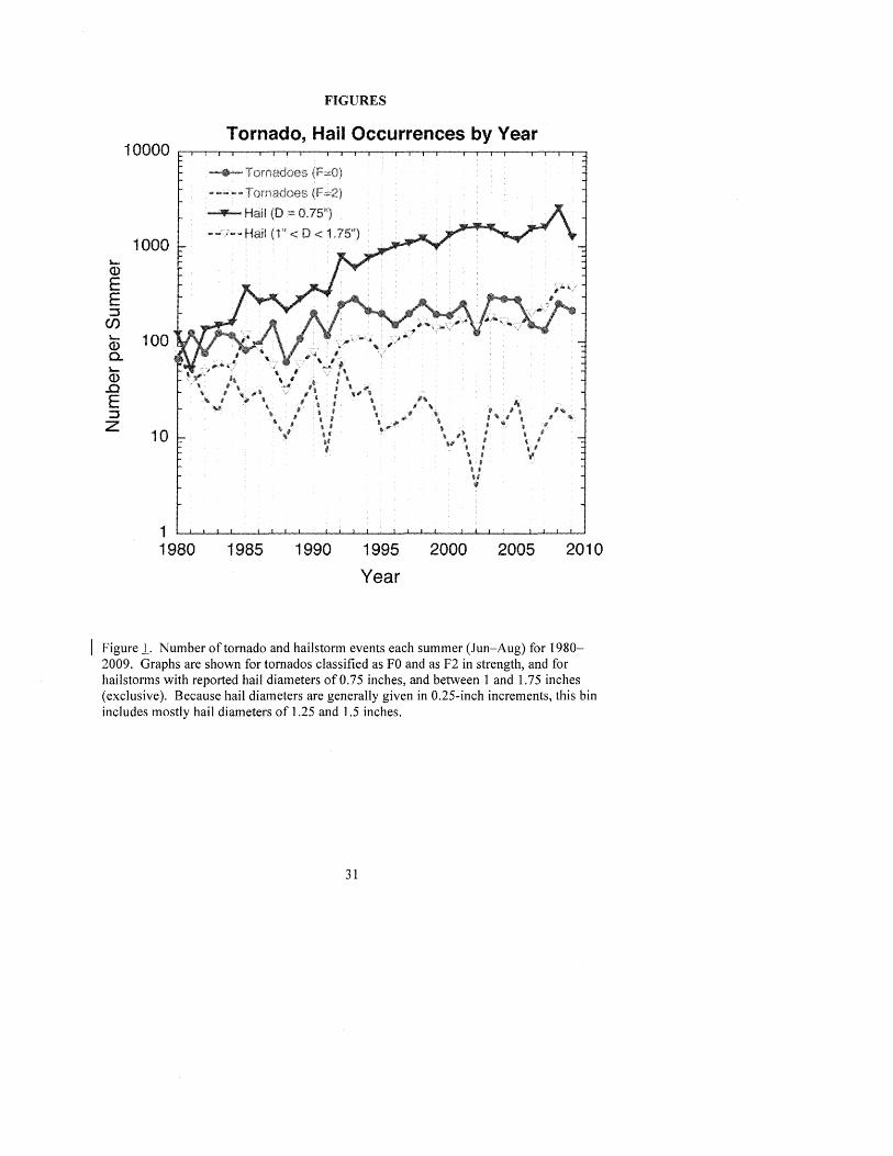
upwards with the years (Figure 1), but the conventions for attributing a given Fujita scale

to a storm have also evolved. Rapid increases in the numbers reported may be due to the

introduction of new technology: implementation of the WSR-88D radars with Doppler

capability in about 1991, for example, may have led to increased reporting of tornados

after that date. An analysis by Ray et al. [2003] suggests that tornados are reported more

often near population centers and that tornado occurrences prior to 1992 may have been

underestimated by about 40%. Contrariwise, Aguirre et al. [1993, 1994] conclude that

some of these "biases" may in fact be caused by environmental changes imposed by

human habitation.

The observational biases that may be present in the data can easily be imagined to

change with the day of the week. Weekly changes in media coverage are possible, for

instance. We argue later in the paper that both the lack of a weekly cycle in the less

populated western half of the U.S. and during the spring season in the eastern half, and

the agreement of the weekly cycle in tornado and hail activity seen in the eastern half

with the weekly cycle seen in other indicators of severe storm activity (indicators that are

not subject to the same concerns about weekly biases in the observational system)

9

suggest that the weekly variations in tornado and hail activity are mostly real and not the

result of weekly shifts in coverage by the observational network.

In preparing the data for analysis, we edited a small fraction of the data entries based

on the recommendations accompanying the data provided by the SPC and on the need to

resolve various ambiguities. Entries with missing state identifications were ignored.

Entries with either zero latitude or longitude locations were ignored. Entries with

negative Fujita scales or hail diameters were ignored. Apparently misidentified time

zones were corrected. Multiple entries associated with a single tornado event were

consolidated into one entry (not an issue in the hail dataset). Tornados that crossed state

boundaries were treated as two separate events, however. Fifteen entries of hail sizes of

0.25 and 0.5 inches in 2007 were pooled with the entries for 0.75 inches. In total, fewer

than 2% of the tornado dataset entries required editing. A far smaller percentage of hail

data entries required editing. The number of tornado events for 1980-2009 in our edited

dataset was approximately 33,000, while the number of hail events was approximately

235,000.

3. The data analysis

In the following subsections we provide details about the assumptions and methods

used in the statistical analysis of the tornado and hailstorm data.

3.1. Statistical model of data under the null hypothesis

10

Testing the data for the presence of a weekly cycle requires a description of the

statistics of the data under the null hypothesis, which is that the frequency of tornados or

hailstorms does not vary cyclically with the day of the week. In modeling the statistics of

hailstorms and tornado occurrences under the null hypothesis, we try to accommodate the

known variations in statistics with the season and year. Our goal is not to determine the

"true" seasonal cycle or decadal trend but simply to produce something likely to be closer

to the truth than ignoring the seasonal cycle or year-by-year trend altogether.

We used the average seasonal cycle over the years 1980-2009 to represent the

modulation of the expected count with the seasons (Le., with the day of the year).

Though we used 15 years of data (1980-1994) prior to the period we are concentrating on

(1995-2009), they were used only to help establish the background seasonal cycles and

decadal-scale trends, and for the bootstrap statistical analysis described later. The

seasonal cycle estimated from 30 years of data is smoother than the cycle estimated using

15 years (1995-2009), as would be expected, but is not substantially different. We

believe that using data prior to 1995-2009 to increase the stability of our estimate of the

seasonal cycle increases the overall robustness of our statistics, but that if we had

confined our averaging to the years 1995-2009 our conclusions would not be changed in

any substantial way.

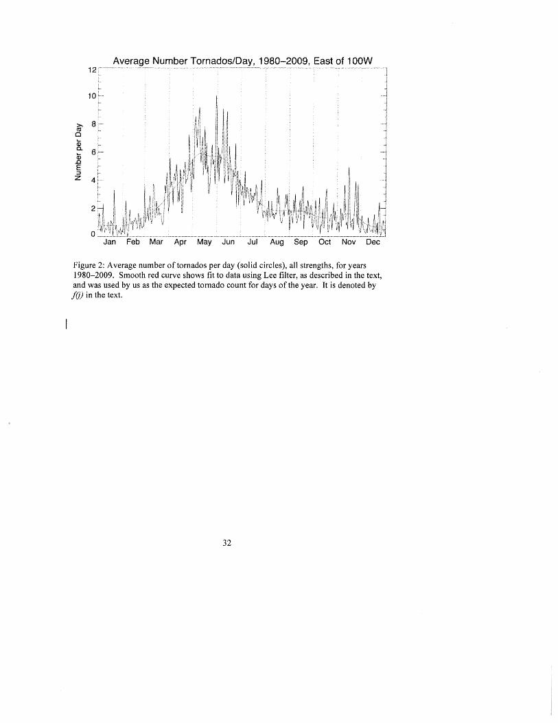
We show in Figure 2 the average number of reported tornados for each day of the

year. The averages for each day of the year in Figure 2 exhibit quite a lot of variability

from day to day, almost certainly due to the sample size (30 samples, one for each year)

in the daily averages. Rather than trying to build a smoother, parameterized model for

the seasonal cycle, we applied a kind of running average to the 365 daily averages (leap

11

years treated as having 365 days). The filter devised by Lee [1986] produced a

satisfactory curve when we applied the filter twice with a window size of 11 days (on

either side of the central value), as shown in Figure 2. The Lee filter produces a smooth

fit to the data but tries also to capture sudden jumps in the local mean.

The annual counts for each year from 1980 to 2009 vary quite a bit from year to year

(e.g., see Figure 1), possibly attributable to large-scale influences such as ENSO or to

sample sizes, but there appears to be a decadal trend in the counts as well. Some of these

trends can be explained by changes in the methods of collecting the data, as mentioned

above.

The seasonal cycles of the different tornado strengths are very similar, we found, as

are the seasonal cycles for different hail sizes, except for overall normalization.

In order to test whether the tornado/hailstorm statistics differ significantly from what

would be expected under the null hypothesis that there is no weekly cycle, we need a

statistical model for the expected number of storms under the null hypothesis. Since we

only test data from particUlar seasons rather than from a full year, we take this into

account in constructing the model. We assume that the expected number of tornado/hail

events for a given day and season/year is proportional to the total number of storms for

that season (thus capturing the interannual variability in Figure 1) and to the average

number of storms for the given day of the year (as represented by the smooth curve in

Figure 2). If there is a weekly cycle, we assume that the cycle is described by a

sinusoidal oscillation multiplying the expected number (Equation 3 below).

12

To represent the expected number of tornados no(y,)) in year y and day j for

summertime tornados (June 1 August 31, i.e., 152 ~j ~ 243) under the null hypothesis,

then, we assume that the number is proportional to the number of tornados that summer

n(y) and to the seasonal cyclefO) represented by the smooth curve in Figure 2. Thus,

. f( j) nOr y,j) = n( y) 243

~ )'-152 f( j')

(1)

If n(y,)) is the actual number of observed storm occurrences in year y for day j,j = 1, ... ,

365 (or 366 in a leap year), we define the ratio variable

r( y,j) = n( y,j)/ nO(y,j), (2)

which has an average very near 1 when averaged over all years of data, or when averaged

over allj, by construction.

A plot (not shown) of the variance of the ratio variable (2) over the 92 days of each

summer vs. the number of tornados for that summer indicates that the variance is fairly

uniform over the years and doesn't seem to vary in a consistent way with the number of

tornados that summer. This suggests that it is reasonable to treat the statistics of the ratio

variable (2) as stationary from year to year.

3.2. Statistical model of weekly cycle

We determine whether there is a weekly cycle in the ratio variable r(y,)) by fitting

the time-dependent data r(t) to a 7-day sinusoid

r(t) = ro + 17 cos[W?( t - Cfi7)] + £(t) (3)

with m-, = 2Jt/(7 days), where ro is the mean of the ratio variable, r7 is the amplitude of the

cycle, and cp, is the time during the week when the weekly cycle peaks. The error in the

13

fit is denoted by crt). The time t is measured in days starting from an arbitrary date

(Tuesday, 1 January 1980, for instance).

It is perhaps worth reminding the reader here that by fitting the data to a pure

sinusoid (Equation 3) we are not assuming that this is in fact an exact description of the

weekly cycle in the data. A periodic signal with period 7 days can always be expressed

as a sum of sinusoids with periods of 7 days and their higher harmonics. The higher

harmonics tend to be noisier and harder to estimate from small amounts of data, and we

have chosen not to examine them. Moreover, because the sinusoid is fit using data from

all days of the week, the sinusoid makes much better use of the data (with more robust

statistics) than a search for a weekly cycle that uses only averages of data from single

days of the week, a practice that is fairly common in searches for weekly cycles in data.

3.3 Statistical tests for weekly cycle

By writing r7 COS[107(t l.p,)] C7 COS(107t) + S7 sin(107t) and using linear-least-squares fits

to this expanded version ofEq. (3) for each week of data, we can use the variance of the

coefficients C7 and S7 from week to week to estimate the overall uncertainty 07 in the

amplitude r7, assuming that the correlation of the coefficients from week to week is

negligible and the number of samples (weeks) for variance estimates is large enough that

.the coefficients are approximately normally distributed. (Time correlations of the fitted

amplitudes from week to week were found to be consistent with the assumed correlation

0.) The ratio (r7/a7i then has a Fisher-Snedecor F distribution with two degrees of

freedom,in the numerator and the number of weeks in the data series in the denominator.

Details of this approach can be found in Bell et ai. (2008). The quantity r7/ a7 is used as a

measure of the signal strength (signal-to-noise ratio). The significance level p of the

14

that

Comment: DANNY: I'll look up a reference as soon as I can get to the library, The distribution is just the classic "F· distribution", r didn't know it was called this until I read a web site about it. Maybe we'll end up calling it the "Fisher" distribution in the

amplitude r7, under the null hypothesis that there is no weekly cycle, can be calculated

from this ratio as

2 P = exp[-(ry /07) ] (4)

as explained in Bell et al. (2008). For example, this means that the probability p that r7 is

larger than 1.73 07 is p 0.05.

Because of the normalization of the observed number n(y,j) by the expected number

no(y,j) in Eq. (2), the value of ro in (3) obtained by the fitting procedure is typically very

close to 1. [It is not exactly 1 because the seasonal cycle f(j) is based on an average over

all years (1980-2009).]

The statistical significance of the amplitude r7 is estimated both by the method

described above and by a second method. The second method of estimating the statistical

significance of the fitted amplitude r7 uses a bootstrap approach in which the original data

are re-sampled in chunks II-days long in a way that destroys any 7-day periodicity in the

original data. Chunk sizes of 11 days are used based on the belief that the correlation of

weekly-cycle fits to the chunks from one chunk to the next is small. Where we have

checked, it is indeed small. To randomize with respect to the day of the week, chunks

are selected that are displaced from the original chunk anywhere from 7 days before to 6

days after the original chunk (i.e., whose starting point is chosen from within a 14-day

window). We choose chunks from prior or future seasons up to 5 years away, instead of

confining ourselves to data from the same year, to increase the number of replacement

choices. Thus, for example, if the chunk we are replacing starts on 10 August 2001, we

may randomly select a chunk from the original dataset beginning anywhere from August

15

3 to August 16 and from any year from 1996 to 2006. This tends to generate simulated

datasets with statistics that change with the day of the year in the same way as the

original dataset, as far as preserving the seasonality of the statistics and decadal trends,

but having no real weekly cycles. Note that because we have access to years prior to

1995, we may select random chunks from years as early as 1990 when a chunk from year

1995 is being replaced. Note that because the statistics of the ratio variable r(y,j) seem to

be fairly constant from year to year, we create simulated datasets starting with the

original dataset for r(y,j) rather than of n(y,j) itself, thereby minimizing the impact of

seasonal and interannual variability on the statistics of the simulated datasets.

Synthesized datasets assembled from the II-day chunks are used to estimate values

of r7 for each dataset, and the statistical significance of the value of r7 obtained from the

original dataset is set at the fraction of synthesized datasets with r7 larger than that of the

original value. We found that the two methods produced comparable significance levels

p (the probability that the value of r7 could equal or exceed its value under the null

hypothesis r7 = 0).

4. Analysis Results

In accordance with the hypothesis that the impact of air pollution on invigorating severe

storms would be greatest in a moist and warm atmosphere, we follow our previous

geographic partitioning [Bell et ai., 2008 and 2009a],. and examine data for the summer

months, June-August, and areas east of lOOW for all latitudes within the USA (our

earlier studies were constrained by the latitudinal coverage of the satellite data we used).

The longitude of 100W separates the moist air mass to the east, where invigoration can be

16

expected, from the dry air masses to the west, where cloud bases are too high and cold to

be substantially invigorated by added aerosols. This is evident in the map of climatic

mean dew point temperature for July, shown in Figure 3a.

Hail and tornado data are available from 1950, but their quality has evolved over

time. The completeness of the coverage has been improving, especially for the weaker

and thus less noticeable events. Observational coverage of tornados seems to have

stabilized since the mid 1990's, whereas coverage of hail appears to have grown

continuously (see Figure 1). We have therefore focused our search on the period 1995-

2009.

A weekly cycle in the aerosol impacts on clouds depends on the existence of a

weekly cycle in anthropogenic aerosols. Such a cycle is observed clearly in Figure 4, in

both PMI0 and PM2.5 (particulate matter concentrations for particle diameters greater

than lO/-lm and 2.5/-lm respectively). The data are collected by the Environmental

Protection Agency (EPA) and are discussed in Bell et al. [2008]. The weekly cycle of hail

and tornadic storms for the years 1995-2009, also shown in Figures 4 and 5, behaves very

similarly to the cycle in the aerosols, with a distinct minimum on weekends.

The temporal and spatial distribution of the weekly cycle matches the distribution of

the warm, moist and unstable conditions in which aerosols have the strongest tendency to

invigorate deep convective clouds [Rosenfeld et al., 2008]. During summer, the longitude

of 100W coincides with the transition from the moist climate to the east of it to the hot

and dry climate to the

17

Comment: I think that it is now fine the way it is. But you are welcome to try your hand and i improve it further. i

Comment: DANNY (4/24/11): Do we need this last sentence here? It refers to figures out of order, and we make the same point later. Also, the following paragraph continues the idea raised in the previous paragraph-if you ignore the last sentence about the behavior of storms west of lOOW, I would suggest deleting this sentence and interchanging Figures 8 and 9, and using the weekly cycles for data west of 100W in Fig, 9 only in the discussion on page 20, about whether there is a weekly bias in observations (as well as pointing out that the lack of a weekly cycle is

with

Deleted: Even though there is a pronounced weekly cycle in aerosols measured by ground­based EPA stations (Figure 7), no significant weekly cycle is apparent to the west of lOOW

Figure~).

The moisture peaks in the months of June, July and August and reaches the northeast

USA, but starts to retreat southward during late August and September. The aerosol

invigoration effect can become apparent in moist atmospheres when synoptic forcing is

less dominant. In cool base clouds (i.e, temperature of about lOoe or less) the effect

might even reverse [Roserifeld et al., 2008]. This is in agreement with the spatial and

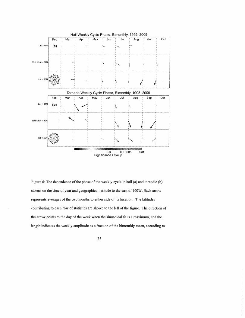
temporal distribution of the weekly cycle, as depicted in Figure 6. The figure shows the

state of the weekly cycle over three latitudinal bands east of lOOW as a function of the

time of year. Each arrow represents the statistics for a bimonthly period and the years

1995-2009. The length of the arrow shows the amplitude of the weekly cycle r7 as a

fraction of the mean rD. The direction indicates the day of the week when the sinusoidal

fit peaks. The color indicates the significance level p of the fit, reflecting the signal-to­

noise ratio of the fit. The figure shows that the transition from the synoptically forced

storms in the ---c.c ........ :: ... : .•.....•.•••• : .. ~ ...•.....•.. ~~ ..••..•.•..... : •.•.••.•.. :: •. : .........•..•••.•.•• ~: •• : ...•.•..•.•....•.•. to the more

locally unstable storms that form in a moist unstable air mass in the summer is

accompanied by an increase in the weekly cycle modulation tending to have a mid-week

maximum. The return of the synoptic forcing and not as moist air in the early fall to the

north part of the domain is similarly associated with a decrease of the weekly cycle there.

Note that the weekly cycle of tornados only becomes established sometime in June, even

though tornadic activity is reaching its peak well before then (See Figure 2). The

consistency of these patterns of occurrence of the weekly cycle in time and space and the

predictions of the hypothesis that the pollution aerosols are the cause of the observed

weekly cycle in severe convective storms lend additional credence to the hypothesis.

18

The overall statistical significance of the weekly cycles of tornado and hail activity

for the IS-year period 1995-2009 is quite high (see caption to Figure 4). We can also

examine the weekly cycle for individual summers based on sinusoidal fits to the data for

each summer alone, though the results are noisy given that there are only 13 weeks in a

summer. The results of such an analysis were displayed in earlier papers as "clock plots"

for rainfall [Bell et al., 2008] and for lightning [Bell et al., 2009a]: the phase and

amplitude of sinusoidal fits were used to plot a point on a clock dial running from

Saturday to Friday and with the distance of the plot point from the center of the plot

proportional to the" signal-to-noise ratio" of the amplitude. The" noise" 07 is

determined from the variance of weekly fits to the data. The signal to noise ratio r7/07 is

given (See Eq. 4) by [-log(P)]112, where p is the significance level of the amplitude r7, i.e.,

the probability that an amplitude this large could have occurred by chance, due to small­

sample effects, when there is in fact no weekly cycle present.

Despite the small number of samples in each summer of data, it was found [Bell et

al., 2009a] that the phases of the weekly cycles in lightning activity for summers between

1998 and 2009 fell year after year in the non-weekend sectors of the clock plot. This

strongly suggests that the weekly cycle in the data has a period of exactly 7 days and is

not an atmospheric wave with a period "in the neighborhood" of 7 days. Because tornado

and hail events are not nearly as numerous as lightning events, and the tornadolhail

observational coverage not nearly as dense, we would expect the year-by-year clock plots

of hail and tornado weekly cycles to be noisier than for lightning. The clock plots for hail

and tornados are shown in Figure,Z. They cover the years 1995-2009. In order to

maximize the weekly cycle signal, only data from the afternoons (1200-2400 local solar

19

9

time), when convective instability is highest, are used in these plots. Though the phases

do not avoid the weekend sectors as completely as the lightning weekly-cycle phases did,

there is still a clear tendency for the weekly cycles of hail storms and tornados to peak in

the middle of the week. When the phase falls on weekends, the signal-to-noise ratio is

quite low, implying that the statistical uncertainty in the determination of the phase is

large. Note that the hail data contain about 7 times as many events as the tornado data

and therefore have more stable statistics, and the phases are more consistent in avoiding

the weekend sectors (Figure 7a).

4.2. Results for tornados west of 100W

not expect to find then: evidence of

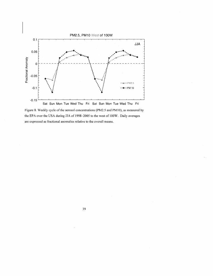
weekly storm invigoratiol\. ~Y€!I1!h()llgh!h€!r€!is(lpr()n()tll1c:e4w€!eklycycle il1 (ler()§()ls ...

measured by ground-based EPA stations west of 100W (Figure 8), no significant weekly

cycle is apparent to the west of 100W (Figure 9).

5. Discussion

The results are in agreement with our previous reports of similar weekly cycles in the

rainfall [Bell et al., 2008] and lightning [Bell et al., 2009a] over the USA. The cycle was

ascribed there to aerosols invigorating deep convective clouds in a warm, moist

atmosphere. It is therefore not too surprising to find that the invigorated clouds also

produce more hail and tornados.

We show in Figure9~Jhat the hail and tornado data are consistent with earlier results

for rain and lightning at the SE U.S. in another respect: when the phase cj>-, and signal

20

Deleted: 9

strength r7 for each summer of data for the years 1995-2009 are displayed on a "clock

plot", there is a clear tendency for the phases to avoid the weekend period, despite the

fact that there are only 13 weeks of data in a single summer and estimates of the weekly

cycle are quite noisy. It is not surprising that the avoidance is not as clear as it was for

the lightning data [Bell et al., 2009a], since lightning occurs far more frequently than hail

storms and tornados and the effective sample size for lightning is far larger.

It is conceivable that the storm data could be affected by a weekly bias in the

observations of storms. However, it is shown in Figures!'~il:il:l1~y)Jthil:tl1()sigl1()fil:

statistically significant weekly cycle in tornado or hail occurrence is visible in the data

west of lOOW. If there is a weekly-varying bias in storm reports it would have to be

present in the eastern half of the U.S. and absent in the western half to explain our results.

Furthermore, the weekly cycle from March to May over the eastern USA (see Figure 6),

is not statistically significant, and no longer point~;ft()allli~:--\V~ek111il:)(ill1111l1~Ifil:l1ythil1g1

it is pointing more towards the weekend, but without any statistical significance. The

signal is too weak to support the possibility of reversal in the convective invigoration

effect in cool base clouds, as hypothesized by Rosenfeld et al. [2008]. The lack of a clear

weekly cycle in the spring along with its existence in the summer, plus the clear

correspondence of the weekly cycle we see in the summer storm data with the cycles

observed in other variables with no possible weekly-varying observational bias, suggests

that the weekly cycle in storms is a real one and not an artifact of the data collection

methods.

The weekly cycle we see is firmly pegged to the work week. It is not plausible that it

is a reflection of a quasi-periodic 7-day cycle in atmospheric dynamics, whose phase

21

would surely wander from year to year something we do not see in any ofthe clock

plots. Kim et al. [2010] recently raised the possibility that the weekly cycle can occur

due to natural random variability [Kim et al., 2010]. This might be the case for a weekly

cycle that is found in general upper tropospheric synoptic features that have no clear

hypothesis to the way that they might be linked to anthropogenic effects [Stinov, 2010].

However, this is not likely to be the case here, based on the lack of evidence of a weekly

cycle in the synoptic properties that correlate with lightning activity that was presented in

the supporting online materials of Bell et al. [2009a]. Previous reports of a weekly cycle

of hail in Southern France [Dessens et al., 2001] did not show a change in hail frequency,

but showed a larger kinetic energy of the hailstones oli weekends. It was postulated that

ice forming nuclei (IFN) emitted during the weekend from the local industry was creating

larger number of ice hydro meteors and therefore decreasing the hailstone sizes due to

greater competition on the available supercooled water. There is no information whether

IFN have a weekly cycle in the eastern USA.

This study has shown a clear relation between the weekly cycle of anthropogenic

aerosols and the occurrences of severe convective storms, which is very unlikely to be a

result of natural variability. The observed associations cannot serve as proof for causality.

However, the results are consistent with the hypothesis that air pollution aerosols

invigorate deep convective clouds in moist and unstable atmosphere, and the possibility

that they can even induce the storms to produce large hail and tornados. Therefore, these

results support this hypothesis. It is worth pointing out that if a roughly 10% weekly

variation in pollution levels is resulting in a simi~ar change in severe storm activity, then

the "background" aerosol level, which is elevated with respect to the pre-industrial level

22

even during weekends, is also likely to be changing the storm frequency we experience

today.

Acknowledgements

Research by DR is an outcome of the European Community-New and Emerging

Science and Technologies (contract 12444 (NEST)-ANTISTORM). Research by TLB

was supported by the Science Mission Directorate of the National Aeronautics and Space

Administration as part of the Precipitation Measurement Mission program under Ramesh

Kakar.

References

Aguirre, B. E., R. Saenz, J. Edmiston, N. Yang, E. Agramante, and D. L. Stuart (1993),

The human ecology of tornadoes, Demography, 30(4), 623-633.

Aguirre, B. E., R. Saenz, J. Edmiston, N. Yang, D. Stuart, and E. Agramante (1994),

Population and the detection of weak tornadoes, Int. 1. Mass Emerg. Disasters,

12(3),261-278.

Andreae M. 0., D. Rosenfeld, P. Artaxo, A. A. Costa, G. P. Frank, K. M. Longo, and M.

A. F. Silva-Dias (2004), Smoking rain clouds over the Amazon. Science, 303, 1337-

1342.

23

Altaratz, 0., 1. Koren, T. Reisin, A. Kostinski, G. Feingold, Z. Levin, and Y. Yin (2008),

Aerosols' influence on the interplay between condensation, evaporation and rain in

warm cumulus cloud. Atmos. Chern. Phys., 8, 15-24.

Bell, T. L., and D. Rosenfeld (2008), Comment on "Weekly precipitation cycles? Lack

of evidence from United States surface stations" by D. M. Schultz et al. Geophys.

Res. Lett .. 35, L09803, doi : 1O.l029/2007GL033046.

Bell, T. L., D. Rosenfeld, K.-M. Kim, 1.-M. Yoo, M.-I. Lee, and M. Hahnenberger

(2008), Midweek increase in U.S. summer rain and storm heights suggests air

pollution invigorates rainstorms, 1. Geophys. Res., 113, D02209,

doi: 10.102912007 lD008623 .

Bell, T. L., D. Rosenfeld, and K.-M. Kim (2009a), Weekly cycle of lightning: Evidence

of storm invigoration by pollution. Geophys. Res. Lett., 36, L23805,

doi: 10.1 029/2009G L040915

Bell, T. L., 1.-M. Yoo, and M.-J. Lee (2009b), Note on the weekly cycle of storm heights

over the southeast United States, 1. Geophys. Res., 114, D15201,

10.1 029/20091DO 12041.

Carbin, G. (2010), Storm Prediction Center WCM Page, URL:

http://www.spc.noaa.gov/wcm/index.htmll\#data.

Dessens, 1., R. Fraile, V. Pont, and 1. L. Sanchez (2001), Day-of-the-week variability of

hail in southwestern France, Atmos. Res., 59, 63-76.

EF: http://www.spc.noaa.gov/efscaie/.

Fan, 1., T. Yuan, 1. M. Comstock, S. Ghan, A. Khain, L. R. Leung, Z. Li, V. 1. Martins,

and M. Ovchinnikov (2009), Dominant role by vertical wind shear in regulating

24

aerosol effects on deep convective clouds, J. Geophys. Res., 114, D22206,

doi: 1 0.1 029/2009JDO 12352.

Fan J, R. Zhang, G. Li, and W.-K. Tao (2007), Effects of aerosols and relative humidity

on cumulus clouds. J. Geophys. Res. 112(D14): D14204.

Foote, G. B. (1984), A study of hail growth utilizing observed storm conditions, J. Clim.

Appl. Meteorol., 23, 84-101.

Gunn R. and B. B. Phillips (1957), An experimental investigation on the effect of air

pollution on the initiation of rain. J. Meteorol. 14,272.

Khain, A. and A. Pokrovsky (2004), Simulation of Effects of Atmospheric Aerosols on

Deep Turbulent Convective Clouds Using a Spectral Microphysics Mixed-Phase

Cumulus Cloud Model. Part II: Sensitivity Study, J. Atmos.ScL, 24, 2983-3001.

Khain, A., D. Rosenfeld, and A. Pokrovsky, (2005), Aerosol impact on the dynamics and

microphysics of deep convective clouds, Q. J. Roy. Meteor. Soc., 131,2639-2663.

Khain, A., N. BenMoshe, and A. Pokrovsky (2008), Factors determining the impact of

aerosols on surface precipitation from clouds: Attempt of classification, J. Atmos.

ScL, 65,1721-1748.

Khain, A., L. R. Leung, B. Lynn, and S. Ghan (2009), Effects of aerosols on the

dynamics and microphysics of squall lines simulated by spectral bin and bulk

parameterization schemes, J. Geophy. Res., 114, D22203,

doi:10.1029/2009JDOl1902.

Khain, A. and B. Lynn (2009), Simulation of a supercell storm in clean and dirty

atmosphere using weather research and forecast model with spectral bin

microphysics, J. Geophy. Res., 114, D19209, doi:l0.1029/2009JDOl1827.

25

Khain, A., O. Rosenfeld, A. Pokrovsky, U. Blahak and A. Ryzhkov (2011), The role of

CCN in precipitation and hail in a mid-latitude storm as seen in simulations using a

spectral (bin) microphysics model in a 20 dynamic frame. Atmos. Res. 99, 129-146.

Kim, K.-Y., R. 1. Park, K.-R. Kim, and H. Na (2010), Weekend effect: Anthropogenic or

natural? Geophys. Res. Lett., 37, L09808, 10.1029/201OGL043233.

Koren 1., Y. 1. Kaufman, O. Rosenfeld, L. A. Remer, Y. Rudich (2005), Aerosol

invigoration and restructuring of Atlantic convective clouds. Geophys. Res. Lett., 32,

L14828, doi: 10.1029/2005GL023187.

Koren 1., 1. V. Martins, L.A. Remer, H. Afargan (2008), Smoke invigoration versus

inhibition of clouds over the Amazon. Science, 15 August, Vol. 321. no. 5891, pp.

946 949.

Koren, 1., L. A. Remer, O. Altaratz, 1. V. Martins, and A. Oavidi (2010), Aerosol-induced

changes of convective cloud anvils produce strong climate warming. Atmos. Chern.

Phys. 10 5001-5010.

Langenberg H. (2011), Triggered lightning. In "news and views", Nature Geosceince, 4,

140.

Lee, 1 .-S. (1986), Speckle suppression and analysis for synthetic aperture radar images,

Opt. Engineer., 25(5), 636-643.

Lee, S. S., L. 1. Donner, and 1. E. Penner (2010), Thunderstorm and stratocumulus: how

does their contrasting morphology affect their interactions with aerosols? Atmos.

Chern. Phys., 10,6819-6837.

26

Lee, S. S., L. J. Donner, V. T. J. Phillips, and Y. Ming (2008a), Examination of aerosol

effects on precipitation in deep convective clouds during the 1997 ARM summer

experiment, Q. J. Roy. Meteor. Soc., l34, 1201-1220.

Lee, S. S., L. J. Donner, V. T. J. Phillips, and Y. Ming (2008b), The dependence of

aerosol effects on clouds and precipitation on cloud system organization, shear and

stability, J. Geophys. Res., 113, D16202, doi: 10.102912007JD009224.

Lerach, D. G., B. J. Gaudet, and W. R. Cotton (2008), Idealized simulations of aerosol

influences on tornadogenesis, Geophys. Res. Lett., 35, L23806,

doi: 10.1029/2008GL035617.

Ludlam, F. H. (1963), Severe local storms: A review, in Severe Local Storms, Meteorol.

Monogr., vol. 27, pp. 1 - 30, Am. Meteorol. Soc., Boston, Mass.

Lyons, W. A., T. E. Nelson, E. R. Williams, J. A. Cramer, and T. R. Turner (1998),

Enhanced positive cloud-to-ground lightning in thunderstorms ingesting smoke from

fires, Science, 282(5386), 77-80, doi:l0.l126/science.282.5386.77.

Markowski, P. M., J. M. Straka, and E. N. Rasmussen (2002), Direct surface

thermodynamic observations within the rear-flank downdrafts ofnontornadic and

tornadic supercells, Mon. Weather Rev., l30, 1692-1721.

Markowski, P. M., J. M. Straka, and E. N. Rasmussen (2003), Tornadogenesis resulting

from the transport of circulation by a downdraft: Idealized numerical simulations, J.

Atmos. ScL, 60, 795- 823.

Molinie J., C. Pontikis (1995), A climatological study of tropical thunderstorm clouds

and lightning frequencies on the French Guyana coast, Geophys. Res. Lett. 22,

1085-1088.

27

Ntelekos, A. A., J. A. Smith, L. Donner, 1. D. Fast, W. I. Gustafson Jr., E. G. Chapman,

and W. F. Krajewski (2009), The effects of aerosols on intense convective

precipitation in the northeastern United States. Quart. J. Roy. Meteor. Soc., 135,

1367-1391.

Ray, P. S., P. Bieringer, X. F. Niu, and B. Whissel (2003), An improved estimate of

tornado occurrence in the Central Plains of the United States, Mon. Weather Rev.,

131(5), 1026-1031.

Rosenfeld D. and C. W. Ulbrich (2003), Cloud microphysical properties, processes, and

rainfall estimation opportunities. Chapter 10 of" Radar and Atmospheric Science: A

Collection of Essays in Honor of David Atlas". Edited by Roger M. Wakimoto and

Ramesh Srivastava. Meteorological Monographs 52, 237-258, AMS.

Rosenfeld D., U. Lohmann, G.B. Raga, C.D. O'Dowd, M. Kulmala, S. Fuzzi, A. Reissell,

M.O. Andreae (2008), Flood or Drought: How Do Aerosols Affect Precipitation?

Science, 321, 1309-1313.

Schaefer, J. T., and R. Edwards (1999), The SPC Tornado/Severe Thunderstorm

Database, in Preprints of the 11th Con/. Appl. Climatology, Dallas, TX.

Snook N., M. Xue (2008), Effects of microphysical drop size distribution on

tornadogenesis in supercell thunderstorms. Geophys. Res. Lett., 35, L24803,

doi: 1O.1029/2008GL035866.

SPC data: http://www.spc.noaa.gov/wcm/index.htmllldata

Stinov S. A. (2010), Weekly cycle of meteorological parameters over Moscow region,

Doklady Earth Sciences, 431,507-513. DOl 10.1 134/S1028334XI0040203.

28

Storer, Rachel L., Susan C. van den Heever, Graeme L. Stephens (2010), Modeling

Aerosol Impacts on Convective Storms in Different Environments. J. Atmos. Sci.,

67, 3904-391S. doi: 10.117S/20101AS3363.1

Tao, W.-K., X. Li, A. Khain, T. Matsui, S. Lang, and 1. Simpson (2007), The role of

atmospheric aerosol concentration on deep convective precipitation: cloud-resolving

model simulations, 1. Geophys. Res., 112, D24S18, doi:l0.1029/2007JD008728.

van den Heever, S. C., and W. R. Cotton (2004), The impact of hail size on simulated

superceII storms, J. Atmos. Sci., 61, 1596- 1609.

van den Heever, S. c., G. G. Carrie, W. R. Cotton, P. J. DeMott, and A. J. Prenni (2006),

Impacts of nucleating aerosol on Florida storms. Part I: Mesoscale simulations. 1.

Atmos. Sci., 63,1752-1775.

van den Heever, S. c., and W. R. Cotton (2007), Urban aerosol impacts on downwind

convective storms. 1. Appl. Meteor. ClimatoI., 46, 828-850

Wang, C. (2005), A modeling study of the response of tropical deep convection to the

increase of cloud condensation nuclei concentration: 1. Dynamics and microphysics,

1. Geophys. Res., 110, D21211, doi:l0.l029/2004JD005720.

Wang 1., S. C. van den Heever, 1. S. Reid (2009), A conceptual model for the link

between Central American biomass burning aerosols and severe weather over the

south central United States. Environ. Res. Lett. 4 01S003 doi: 10.1088/1748-

9326/4/1/01S003.

Williams, E. R. (2005), Lightning and climate: A review, Atmos. Res., 76(1-4), 272-287,

doi:10.1016/j.atmosres.2004.11.014.

29

Williams, E., O. Rosenfeld, M. Madden et al. (2002), Contrasting convective regimes over the

Amazon: Implications for cloud electrification. J. Geophys. Res., 107 (020),8082,

doi: 10.1029/2001 J 0000380.

Williams, E., and S. Stanfill (2002), The physical origin of the land-ocean contrast in lightning

activity, C. R. Phys., 3(10), 1277-1292, doi:10.1016/S1631-0705(02)01407-X.

Yuan T., L. A. Remer, K. E. Pickering, and H. Yu (2011), Observational evidence of aerosol

enhancement of lightning activity and convective invigoration. GRL, 38, L04701,

doi: 1 0.1 029/201 OGL046052.

30

:0-

m E E :J

C/) :0-

m a. :0-

m ..0 E :J Z

FIGURES

Tornado, Hail Occurrences by Year 10000 ~~~~~~~~~~~~~~~~~~

1000

100

10

1 1980 1985 1990 1995

Year

2000 2005 2010

Figure Number of tornado and hailstorm events each summer (Jun-Aug) for 1980-2009. Graphs are shown for tornados classified as FO and as F2 in strength, and for hailstorms with reported hail diameters of 0.75 inches, and between 1 and 1.75 inches (exclusive). Because hail diameters are generally given in 0.25-inch increments, this bin includes mostly hail diameters of 1.25 and 1.5 inches.

31

Average Number Tornados/Day, 1980-2009, East of 100W 12,

~ 10 L __ --J

~ 8 cu 0 (5 0. 6 .... ~ E ::J Z 4

2

0

Figure 2: Average number of tornados per day (solid circles), all strengths, for years 1980-2009. Smooth red curve shows fit to data using Lee filter, as described in the text, and was used by us as the expected tornado count for days of the year. It is denoted by 10) in the text.

32

:J

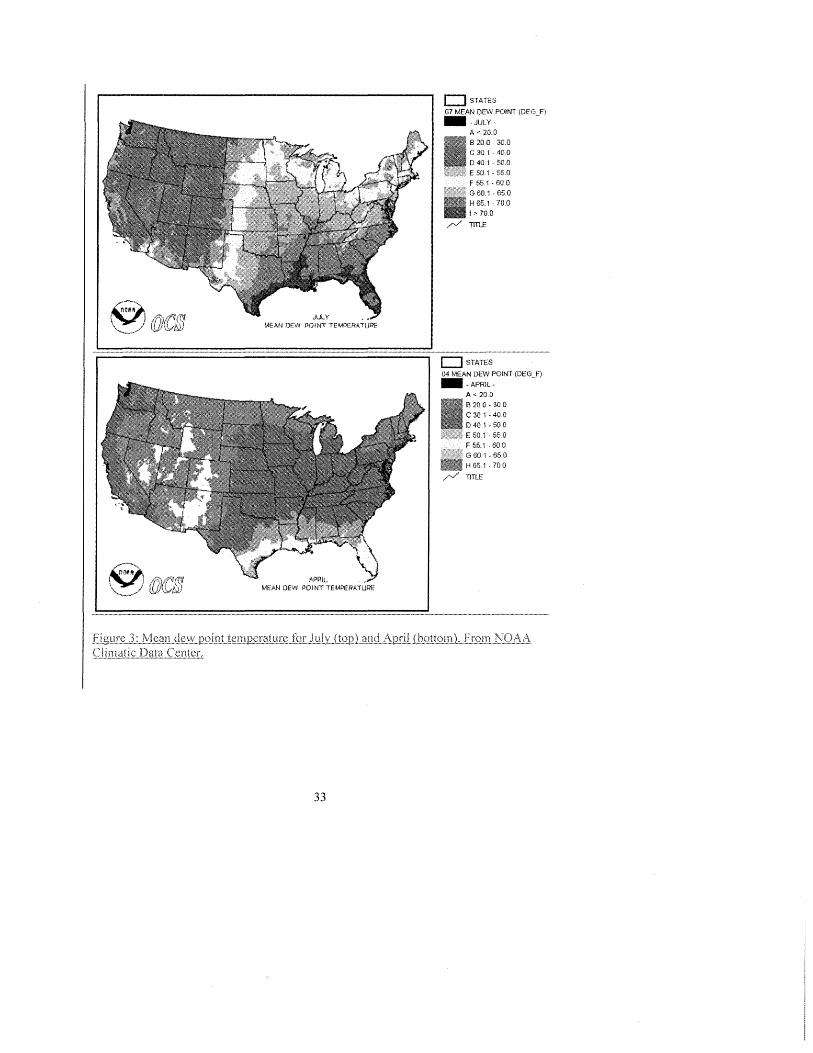
33

CJ POINT 01 MEAN -A <:: 2(10 B

Figure 1: A weekly cycle of the aerosols (PM2.5 and PMIO), as measured by the EPA

over the USA during JJA of 1998-2005 to the east of 100W, along with the associated

weekly cycle of the SPC-reported hail storms and tornados over the same area averaged

over JJA for 1995-2009. The significance levelp for the weekly cycle of tornados is p =,

0.011 (F-test) and p 0.033 (bootstrap test). The significance level for the hail data is p

= 0.00013 (F-test) and p = 0.0008 (bootstrap test with 104 simulated datasets).

34

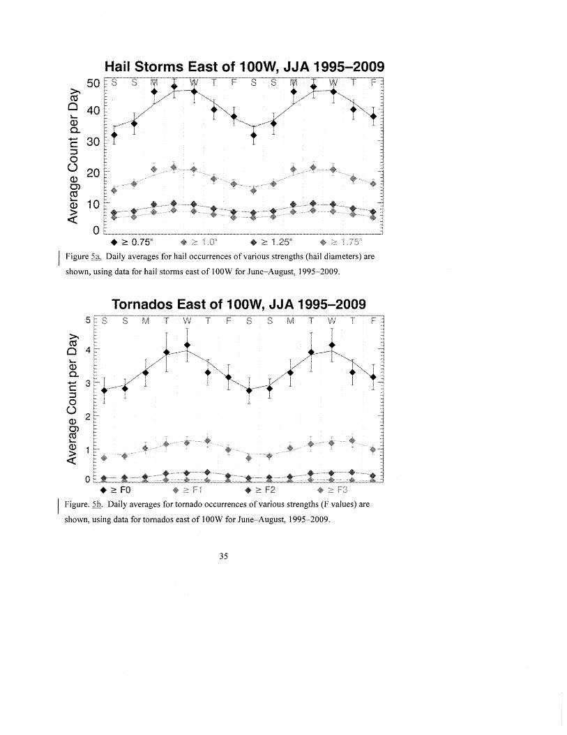
Hail Storms East of 100W, JJA 1995-2009 50

~ co 0 40 \-(j) a.. .... 30 c:: :::J 0 () 20 (J.) 0) ctS \-

10 (j)

~ 0

.;::: 0.7511 ,. ~ 1

Figure Daily averages for hail occurrences of various strengths (hail diameters) are

shown, using data for hail storms east of lOOW for June-August, 1995-2009.

Tornados East of 100W, JJA 1995-2009 5

~ co Cl 4 l....

<D a.. ....... 3 c: :::J 0 ()

2 <D g \-

<D

~ 0

Figure. Daily averages for tornado occurrences of various strengths (F values) are

shown, using data for tornados east of 100W for June-August, 1995-2009.

35

Hail 1995-2009 Feb Mar Aug Sep Oct

Figure 6: The dependence of the phase of the weekly cycle in hail (a) and tomadic (b)

storms on the time of year and geographical latitude to the east of lOOW. Each arrow

represents averages of the two months to either side of its location. The latitudes

contributing to each row of statistics are shown to the left of the figure. The direction of

the arrow points to the day of the week when the sinusoidal fit is a maximum, and the

length indicates the weekly amplitude as a fraction of the bimonthly mean, according to

36

the key at the bottom left of the figures. The radius of the outermost circle in the key

represents a fractional anomaly of 0.15. The arrows are colored according to their

significance level, with the color_bar below indicating the significance level assigned to

each color.

37

Annual Phase, Significance of Hail Weekly Cycle

(a) Sun

Tornado Weekly Cycle (b) Sun

Fri Tue

1995-2009 Afternoon

Figure 7: The phase (day of the week) and amplitude of the weekly cycle (Eq. 1) of data

for each summer for the years 1995-2009. The amplitude is represented by the distance

from the origin and is proportional to the signal-to-noise ratio of the amplitude, r7/a;.

The last two digits of the year are shown in the colored balloons. The probability p that

the amplitude of the weekly cycle could exceed a given radius, under the null hypothesis

r7 0, is shown by the circles labeled by the corresponding value ofp. (a) Hail data. (b)

Tornado data.

38

PM2.5, PM10 of 100W 0.1

JJA

0.05"

>. 1i3 E 0 0 c «

1i3 c 0 ·0.05 13 ~ u..

-0.1

-0.15 Sat Sun Mon Tue Wed Thu Fri Sat Sun Mon Tue Wed Thu Fri

Figure 8. Weekly cycle of the aerosol concentrations (PM2.5 and PMIO), as measured by

the EPA over the USA during JJ A of 1998-2005 to the west of 1 OOW. Daily averages

are expressed as fractional anomalies relative to the overall means.

39

of 100W, JJA 1995-2009 20

~ co 0 '- 15 (]) 0. ...... c: :::J 10 0 0 (]) 0> co 5 t.-(]) > «

0 • ;::: 0.75" 1.2511

Figure 9a. Daily averages for hailstorm occurrences of various strengths (hail diameters)

are shown, using data for hail storms west of lOOW in JJA and for 1995-2009. The

weekly cycles are not statistically significant.

~ 1.5 CO o t.-(])

0. 1.0 ...... c: :::J o o (]) 0> 0.5 CO t.-O)

~

of 100W, JJA 1995-2009

Figure 9b. Daily averages for tornado occurrences of various strengths (EF values) are

shown, using data for tornados west of lOOW in JJA and for 1995-2009. The weekly

cycles are not statistically significant.

40