why are we learning/developing this mathematics?
TRANSCRIPT
Why are we learning/developing this
mathematics?
Two major scientific developments of the past 50 years:
• Complexity of nonlinear dynamical systems
• Development of information technologies
1

Structural stability is not generic
Homoclinic tangencies
• Newhouse Phenomenon - strange attractors and arbitrarily
long stable periodic orbits intertwined in parameter space.
2

Structures or patterns at multiple scales
• Chaos
• Continuously changing patterns
3

Structures or patterns at multiple scales
• Turbulence - spatial-temporal chaos
4

Structures or patterns at multiple scales
• Fractals - topography
5
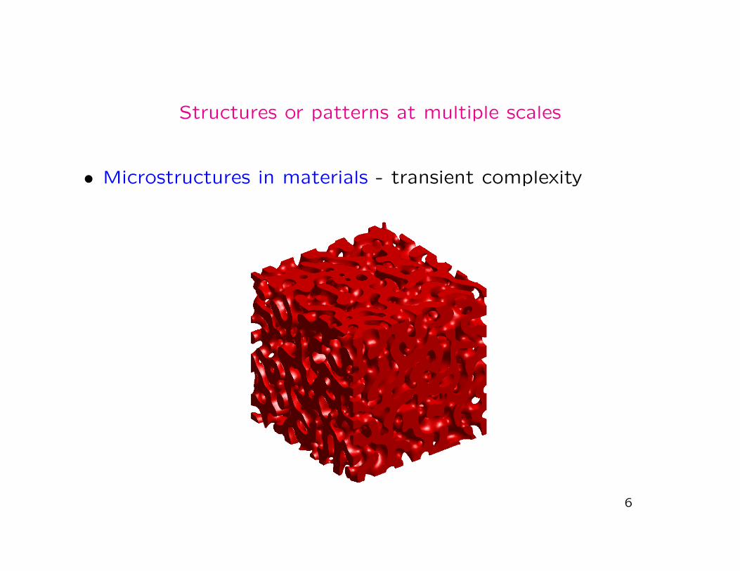
Structures or patterns at multiple scales
• Microstructures in materials - transient complexity
6
We need rigorous mathematical techinques that can do two
things:
• Capture those structures that persist under perturbation.
• Identify structures down to a particular scale.
7

Conley theory (topological generalization of Morse theory) pro-
vides us with appropriate tools.
8

Conley theory (topological generalization of Morse theory) pro-
vides us with appropriate tools.
I. Structure Theorems
• Existence of periodic orbits
9
Conley theory (topological generalization of Morse theory) pro-
vides us with appropriate tools.
1. Structure Theorems
• Existence of periodic orbits
• Structure of connecting orbits
10

Conley theory (topological generalization of Morse theory) pro-
vides us with appropriate tools.
1. Structure Theorems
• Existence of periodic orbits
• Structure of connecting orbits
• Existence of symbolic dynamics
11
Conley theory (topological generalization of Morse theory) pro-
vides us with appropriate tools.
1. Structure Theorems
• Existence of periodic orbits
• Structure of connecting orbits
• Existence of symbolic dynamics
• Existence of homoclinic tangencies
12
Conley theory (topological generalization of Morse theory) pro-
vides us with appropriate tools.
1. Structure Theorems
• Existence of periodic orbits
• Structure of connecting orbits
• Existence of symbolic dynamics
• Existence of homoclinic tangencies
• Singular perturbations
13

Conley theory (topological generalization of Morse theory) pro-vides us with appropriate tools.
1. Structure Theorems
• Existence of periodic orbits
• Structure of connecting orbits
• Existence of symbolic dynamics
• Existence of homoclinic tangencies
• Singular perturbations
• Time series14
2. Bifurcation Theorems
• Homoclinic and heteroclinic orbits
15

2. Bifurcation Theorems
• Homoclinic and heteroclinic orbits
• Resolution or Data Compression
16
2. Bifurcation Theorems
• Homoclinic and heteroclinic orbits
• Resolution or Data Compression
• Computer Graphics
17

18

Limiting factors in applying the Conley index
1. Finding index pairs
19

Limiting factors in applying the Conley index
1. Finding index pairs
2. Computing the Conley index
20
Computer Assisted Proof in Dynamics
1. Chaotic dynamics in Lorenz equations
21
Computer Assisted Proof in Dynamics
1. Chaotic dynamics in Lorenz equations
2. Homoclinic tangencies in Henon
22

Computer Assisted Proof in Dynamics
1. Chaotic dynamics in Lorenz equations
2. Homoclinic tangencies in Henon
3. Infinite Dimensional Systems
• Bifurcation diagrams (Swift-Hohenberg, Kuramoto-Sivashinsky,
FitzHugh-Nagumo)
23

0.3 0.4 0.5 0.6 0.7 0.8 0.9 10
0.05
0.1
0.15
0.2
0.25
0.3
0.35
0.4
0.45
0.5
M(1+)
M(2+)
M(0)
ut = E(u) =
ν −(1 +
∂2
∂x2
)2u − u3, u(·, t) ∈ L2
(0,
2π
L
),
u(x, t) = u
(x +
2π
L, t
), u(−x, t) = u(x, t), ν > 0, (1)
24
Computer Assisted Proof in Dynamics
1. Chaotic dynamics in Lorenz equations
2. Homoclinic tangencies in Henon
3. Infinite Dimensional Systems
• Bifurcation diagrams (Swift-Hohenberg, Kuramoto-Sivashinsky,
FitzHugh-Nagumo)
• Global attractors for gradient systems (Swift-Hohenberg)
25

Computer Assisted Proof in Dynamics
1. Chaotic dynamics in Lorenz equations
2. Homoclinic tangencies in Henon
3. Infinite Dimensional Systems
• Bifurcation diagrams (Swift-Hohenberg, Kuramoto-Sivashinsky,
FitzHugh-Nagumo)
• Global attractors for gradient systems (Swift-Hohenberg)
• Chaotic dynamics (Kot-Schaffer)
26

Computer Assisted Proof in Dynamics
1. Chaotic dynamics in Lorenz equations
2. Homoclinic tangencies in Henon
3. Infinite Dimensional Systems
• Bifurcation diagrams (Swift-Hohenberg, Kuramoto-Sivashinsky,FitzHugh-Nagumo)
• Global attractors for gradient systems (Swift-Hohenberg)
• Chaotic dynamics (Kot-Schaffer)
4. Geometric approximations of vector fields.
27

Conley Index
f : X → X a continuous function on a locally compact metric
space
S ⊂ X is invariant if for every x ∈ S there exists a full trajectory
γx : Z → S such that
γx(0) = x, and γx(n + 1) = f(x).
N ⊂ X is an isolating neighborhood if
Inv(cl(N), f) := {x ∈ N | ∃ γx : Z → N} ⊂ int(N)
28

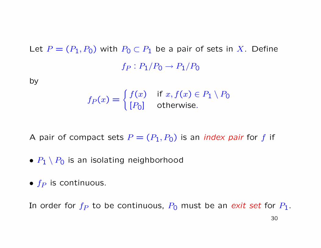
Let P = (P1, P0) with P0 ⊂ P1 be a pair of sets in X. Define
fP : P1/P0 → P1/P0
by
fP (x) =
{f(x) if x, f(x) ∈ P1 \ P0
[P0] otherwise.
29
Let P = (P1, P0) with P0 ⊂ P1 be a pair of sets in X. Define
fP : P1/P0 → P1/P0
by
fP (x) =
{f(x) if x, f(x) ∈ P1 \ P0
[P0] otherwise.
A pair of compact sets P = (P1, P0) is an index pair for f if
• P1 \ P0 is an isolating neighborhood
• fP is continuous.
In order for fP to be continuous, P0 must be an exit set for P1.
30

Theorem: (Wazewski Principle) If fP is not homotopically trivial,
then
Inv(cl(P1 \ P0), f) 6= ∅.
31

Theorem: (Wazewski Principle) If fP is not homotopically trivial,
then
Inv(cl(P1 \ P0), f) 6= ∅.
Remark: Homotopy theory is hard to compute with.
32
Theorem: (Wazewski Principle) If fP is not homotopically trivial,
then
Inv(cl(P1 \ P0), f) 6= ∅.
Remark: Homotopy theory is hard to compute with.
Theorem: (Wazewski Principle) If
fP∗ : H∗(P1/P0, [P0]) → H∗(P1/P0, [P0])
is not nilpotent, then
Inv(cl(P1 \ P0), f) 6= ∅.
33

Shift Equivalence
The homology Conley index of Inv(cl(P1 \ P0), f) is the shift
equivalence class of fP∗ : H∗(P1/P0, [P0]) → H∗(P1/P0, [P0]).
Two group homomorphisms f : X → X and g : Y → Y are shift
equivalent if there exist group homomorphisms r : X → Y and
s : Y → X and a natural number m such that
r ◦ f = g ◦ r, s ◦ g = f ◦ s, r ◦ s = gm, s ◦ r = fm
34

Prop: Let f : X → X and g : Y → Y be group homomorphisms
that are shift equivalent. Then f is nilpotent if and only if g is
nilpotent.
Proof: Assume f is not nilpotent. Since s◦ r = fm, neither r nor
s are trivial. Assume that gk = 0. Then
r ◦ f = g ◦ r,
s ◦ r ◦ f ◦ (s ◦ r)k = s ◦ g ◦ r ◦ (s ◦ r)k,
fm ◦ f ◦ (fm)k = s ◦ g ◦ (r ◦ s)k ◦ r,
fm(k+1)+1 = s ◦ g ◦ (gm)k ◦ r,
fm(k+1)+1 = 0.
This contradicts the assumption that f is not nilpotent.
Exercise: f(x) = 2x is not shift equivalent to g(x) = x.
35