!

WHY ARE POOR COUNTRIES POOR? !

Daniel Cohena and Marcelo Sotob

First version: October 2002This version: December 2003

ABSTRACT

We attempt to explain why standard explanations of the poverty of nations areunsatisfactory. We first argue that human capital is low in poor countries because its productionhas increasing returns with respect to life expectancy. We then show that the reason why capitaldoes not flow to poor countries (the Lucas paradox) can readily be explained once market pricesrather than PPP prices are used to assess the return to capital. We finally argue that PPPcalculations bias downwards the measured TFP of poor countries, which may in part explain theirlower productivity. The message of hope is that education can shoot up as life expectancyincreases, while physical capital could flow in as the real exchange rate appreciates.

JEL classification: F21; J24; O47; P36

"""""""""""""""""""""""""""""""""""""""""""#" The authors would like to thank Paul David, Kenneth Rogoff and Jorge Braga de Macedo for stimulatingdiscussions on the ideas presented here. The views expressed in this paper do not necessarily represent those of theOECD.

a Ecole Normale Supérieure and OECD Development Centre. E-mail : dcohen@elias.ens.fr

b Institute for Economic Analysis. E-mail : marcelo.soto@iae.csic.es

$

I. Introduction

Why are poor countries poor? A wide ranging number of answers have been offered to thisquestion. Within the Solow framework, three usual suspects have been rounded up: physicalcapital, human capital, and total factor productivity. Scarcity of physical capital, first, has beenrapidly disregarded as a cause of poverty because no externalities seem to exist and capitalmobility worldwide would meet capital shortage (see, among others, Easterly, 1999). Humancapital has also been progressively discarded: again, externalities seem to be very low orinexistent (see Heckman and Klenow, 1997, or Krueger and Lindahl, 2001) and the contributionof human capital to growth appears to be too small to explain the gap between rich and poornations (see, among others, Bils and Klenow, 2000). One could also add that migrant workersearn much more in rich countries than in their home countries, so that human capital cannot be, inisolation, the reason why poor countries are poor. Eventually, only one suspect appears to survive:total factor productivity, which lends itself to the analysis of other kinds of explanatory variablessuch as institutions or “social infrastructure” as they are called in Hall and Jones (1999).

However, in our view, there is no single factor explaining poverty. Rather than looking forthe one big story about the roots of poverty, one needs to explain each of the bits of thedevelopment puzzle. In section II we show that while the middle- and low-income countriesexcluding sub-Saharan Africa have one third of the rich countries’ income per head, each of thethree items of the production function –physical capital, human capital and total factorproductivity– represent on average 70 per cent of the levels attained by rich countries. Similarly,sub-Saharan African countries stand at about one tenth of the rich countries’ income level. Yeteach of the three items are worth about 50 per cent of the rich countries’ levels. This is why weargue that poverty cannot be understood by focusing on just one item but rather we have toaddress the handicaps in each of these items. In the paper we attempt to explain the origins ofthese handicaps.

We first address human capital. A Becker/Mincer model would characterize education asan investment that should critically depend on the time horizon on which it is recouped, namelyon life expectancy. However, a simple calculation shows that since 1960, every year increase inlife expectancy is associated with a rise of more than half a year of schooling in rich countries, butonly one third of a year of schooling in poor countries. So, why the reduction of worldwideinequalities in life expectancy has not been channelled into a convergence of educationalattainment across the world (the Becker paradox, as we shall call it)? The answer is relativelystraightforward: both the theory and the data point to a non-linear relationship between educationand life expectancy. In section III we show that in a standard Mincerian approach the decision onschooling is a convex function of life expectancy, which is why the marginal propensity to investin education rises with life expectancy. In section IV we show empirically that this is indeed thecase, with education rising significantly only when life expectancy at the age of 5 is above 50years. As a result, the poorest countries are only in the early stage of their educational formation.

In section V we address the Lucas paradox, i.e. the fact that in spite of capital mobility andapparent differences in the rates of return between rich and poor countries, capital does not flowto poor countries. We argue that the paradox arises from a misuse of the Summers-Heston data.

%

While these data are certainly very useful for analysing income per head, they cannot be used forgauging the return to physical capital. The proper way to calculate the relative return of capital isto use domestic prices instead of PPP prices. Indeed, the use of PPP prices overestimates the valueof marginal productivity of physical capital in poor countries. As we shall see in Section V, thecapital output ratios are actually amazingly similar across the world when market prices are used.In other words, there is simply no Lucas paradox when the returns to capital are appropriatelymeasured. By this we do not mean that other factors such as country risk are not important indetermining the return to capital. Instead we argue that a proper measure of the returndramatically reduces differences across countries.

Finally, one additional implication that we shall draw from this analysis refers to totalfactor productivity. We will argue that growth accounting based on Summers-Heston data is likelyto bias the measurement of TFP. Indeed, to the extent that the efficient allocation of resources in apoor country is channelled towards the sector which has a relative high market price, this countrywill not necessarily allocate its resources in the sectors that would be dictated by PPP prices,hence a low TFP level. The inefficiency revealed by TFP may then be exaggerated.

The message of hope that one may then draw from this paper is that a virtuous circle maywell be starting sometime soon in poor countries. The progress of life expectancy, if (a big if) itwas to be maintained, would increase the investment in education. This would have larger effectson human capital accumulation than it did in the past as non-linearities start to operate.Furthermore, as these countries get richer, the price of non-traded goods would rise. This priceincrease would raise the profitability of capital, thus eventually attracting more investment fromabroad. In the next section we show that factor accumulation is indeed important for economicdevelopment, as opposed to the findings of the recent literature.

II. THE ROLE OF FACTOR ACCUMULATION

II.1 Income levels

Let us write aggregate output ( itQ ) of country i at time t as a Cobb-Douglas function of

human and physical capital ( itH and itK respectively) and total factor productivity ( itA ):

α−α= 1itititit HKAQ (1)

This equation is now the received workhouse of growth models. Before analysing thedeterminants of each of these three items, it is useful to look at the gaps in these items betweenrich and poor nations implied by the production function. The earlier literature has done thisaccording to different approaches. Our preferred approach amounts to write output per head as theproduct of three terms: human capital, the ratio of physical to human capital with an exponent ofα and total factor productivity (we explore other alternatives below). Setting α = 1/3 and the

&

average of high-income countries in each of one these terms equal to one!, we obtain thefollowing results:

Table II.1a Contribution of Human and Physical Capitaland Total Factor Productivity to Income

Output per head Human CapitalPhysicalCapital

Total FactorProductivity

Rich countries 1 1 1 1Middle- and low-income countries excluding SSA 0.35 0.65 0.69 0.75Sub-Saharan Africa (SSA) 0.11 0.49 0.41 0.48

Note: According to the decomposition LHHKALQ /3/1

)/(/ = in which Q/L is output per head, H is human capital, K is

physical capital: each term is divided by the average of rich countries’ levels.Source: Cohen and Soto (2001), for Human Capital; Easterly and Levine (2001), for physical capital; Penn World Table 5.6 for output.

Table II.1a is an amazing illustration of the power of multiplication. While the middle- andlow-income countries excluding sub-Saharan Africa stand at about one third of the rich countries’income per head, each of the three items are about 70 per cent (only) of the level of rich countries.But 70 per cent to the power of three is 35 per cent! Similarly, the average income level in sub-Saharan Africa is only one tenth of rich countries’ income level. However each of the threecomponents of the production function is between 40% and 50% the levels observed in richcountries. Multiplying small or relatively benign handicaps can yield a dramatic effect on acountry’s income. This decomposition explains why, in our view, single factor explanations of thepoverty of nations are usually found to be unsatisfactory. Neither human nor physical capitalalone can explain much. This is also why many authors have argued that differences in total factorproductivity are the main source of disparities in income across countries. Table II.1 suggestsinstead why the “transpiration” strategy of Singapore, which focused on human and physicalcapital, worked: by fixing two out of three items, a country can go a long way towards solving itsdevelopment problem. Krugman (1994) referred to the “transpiration” strategy of Singaporeechoing Edison’s famous remark that it takes more transpiration than inspiration to innovate.Singapore’s strategy is indeed one in which most of the growth has appeared to be driven byfactor accumulation (in human and physical capital) rather than by total factor productivity (seeYoung, 1995). The table also gives a hint on why migrant workers do well abroad: their humancapital allows them to double their income as they move from middle- and low-income countries(excluding sub-Saharan Africa) to rich countries, and to multiply it by five if they come from sub-Saharan Africa.

The income decomposition presented above gives a lower role to TFP than most readers ofthe Hall and Jones (1999) paper would expect. One reason is that our decomposition is slightlydifferent from the one presented by Hall and Jones, who prefer to rewrite the output per worker asa function of the capital-output ratio:

)/()/(/ 1/1/1ititititititit LHQKALQ ααα −−=

"""""""""""""""""""""""""""""""""""""""""""1 Table A1 in the appendix shows the countries used in this paper

'

Table II.1b. Decomposition à la Hall-Jones

Q/L (K/Q)0.5 H A1.5

Rich Countries 1 1 1 1Middle- and low-income countries excluding SSA 0.35 0.81 0.65 0.67Sub-Saharan Africa (SSA) 0.11 0.60 0.49 0.35

However, Hall and Jones’s decomposition inflates the role of total factor productivity inexplaining differences in output across countries (Table II.1b). This is so because they raise theTFP to the power 1.5 and make comparisons with this new definition of TFP. This obviouslyexacerbates differences in productivity across countries. Hall and Jones argue that decomposing interms of the capital-output ratio is more relevant than the capital-labour ratio because in the longrun the capital-output ratio is constant. As our discussion of the Lucas paradox will show, this isnot the case.

At any rate, our decomposition is not widely different from the one used by Hall and Jone.Taking physical and human capital together, factor accumulation has a larger explanatory powerthan TFP in explaining the poverty of nations. This contradicts the now received idea that factoraccumulation could not explain growth. The earlier and most influential papers on this areBenhabib and Spiegel (1994), Bils and Klenow (2000), Klenow and Rodriguez-Clare (1997), andEasterly and Levine (2001). We review critically the arguments given against the role humancapital in a companion paper (Cohen-Soto, 2001). There we argue, along Krueger and Lindahl(2001), that measurement errors are too large, which is why increases in education do not seem tobe significant in growth regressions.

The tables above presented describe the average differences in each of the three terms ofthe production function between countries. But averages may mask the underlying causes ofpoverty. For instance, some developing countries may have a relatively high TFP and others arelatively low one, which would result in an average TFP “not so different” from rich countries’.Therefore, instead of looking at averages, one could compare the richest country with the poorestones, as Hall and Jones (1999) do. But this is an extreme way to proceed too. An intermediaryapproach to evaluate the contribution of factor accumulation is through the variancedecomposition of the output level, as done by Klenow and Rodriguez-Clare (1997) and Easterlyand Levine (2001). Klenow and Rodriguez-Clare make a variance decomposition of the incomelevel across countries similar to:

( ) ( )( ) ( )( ) ( ) ( )( ) ( )( )itititititit qLogVarTFPLogqLogCovqLogVarxLogqLogCov ;;1 += (2)

where lowercases represent variables in per worker terms and xit is an aggregate of total factoraccumulation per worker, defined as:

3/23/1 hkx =

(

Decomposition (2) is different from the one used by Klenow and Rodriguez-Clare (1997).There the production function is expressed in terms of the capital-output ratio. Suchdecomposition would be justified if the capital-output ratio were constant. However it is a well-known fact that, at PPP prices, rich countries tend to have higher capital-output ratios than poorcountries. In addition, the estimation of the contribution of the capital-output ratio in total outputwill be necessarily biased downwards. For these reasons we opt for decomposing incomeaccording to the expression (2). As Klenow and Rodriguez-Clare point out, the first term of thisexpression corresponds to the coefficient obtained in an OLS regression of log(xit)t on log(qit) anda constant and so it can be interpreted as the expected increase in log(xit) given and increase inlog(qit). Table II.2 shows the results of this decomposition. The numbers are qualitatively similarto those of Table II.1. Namely, factor accumulation explains more than 60% of the variance of theoutput level. Moreover, this figure has been fairly stable over the period 1960-1990.

Table II.2. Variance decomposition of the income level per worker

Decomposition à la Klenow-Rodriguez Decomposition à la Easterly-Levine

Factor Accumulation TFP FactorAccumulation

TFP Covariance

1960 0.64 0.36 0.48 0.20 0.32

1970 0.63 0.37 0.47 0.20 0.33

1980 0.65 0.35 0.49 0.19 0.32

1990 0.62 0.38 0.44 0.19 0.37

Easterly and Levine (2001) further decompose (2) in order to account for the covariancebetween factor accumulation and TFP. This is important because part of the contribution of factoraccumulation may be induced by TFP improvements. We consider the covariance in the followingexpression2,

( )( ) ( )( ) ( )( ) ( )( )( ) ( )( ) ( )( )ititit

itititit

qLogVarTFPLogxLogCov

qLogVarTFPLogVarqLogVarxLogVar

;2

1

×++=

(3)

The last three columns of Table II.2 present the main results of the Easterly-Levinedecomposition. The variance of factor accumulation alone explains between 40% and 50% of the

"""""""""""""""""""""""""""""""""""""""""""2 Easterly and Levine assume decreasing returns in x, which implies a slightly different formulation for (3). Howeverthe hypothesis of decreasing returns is rejected by the data (see Soto, 2002).

)

output variance. TFP alone explains around 20% and the remaining 30% to 40% is explained bythe covariance between factors and TFP. Overall, it is hard to argue from these numbers that TFPis the main determinant of income differences across countries. The role of factors of productionis at least as important as TFP’s.

II.2 Income growth

Traditionally the literature has emphasised the differences in output growth rather thandifferences in the output level. Pritchett (2001) and Easterly and Levine (2001) have argued thatdiscrepancies in the growth rate of human and physical capital are not able to explaindiscrepancies in the growth rate of output per worker across countries. This may be in part due tomeasurement error (Krueger and Lindahl, 2001) or collinearity between both types of capital(Soto, 2002). We explore here the significance of the change in capital stocks with a simpleregression of output growth on ∆x and time dummies over the period 1960-1990 (data are for thebeginning of each decade). Column 1 of Table II.3 shows the OLS estimate, which results in acoefficient 50% higher than the value that could have been expected (i.e. one). This is due to theendogeneity of factor accumulation. The R2 is also very high, but it is certainly biased upwards forthe same reason. The second column is obtained by using lagged changes of x as instruments. Weget a coefficient which perfectly fits the expected value, namely one. Columns 3 and 4 replicatethe regressions but constraining the coefficient on ∆x to one. The R2 is still high, although it fallsslightly when the time dummies are dropped (column 4). Globally, these simple regressions showthat factor accumulation is a significant determinant of output growth.

Table II.3. Regression of income growth on factor accumulation (1960-1990)(Dependent variable is dlog(output per worker))

(OLS)(1)

(IV)*(2)

(OLS; constrained)(3)

(OLS; constrained)(4)

Factor Accumulation1.57

(0.142)1.02a

(0.536)1.00 1.00

R2 0.601 - 0.553 0.439

Observations 230 147 230 230

83 countries; data at the beginning of each decade; time dummies included, except for column 4; WhiteHeteroskedasticity-consistent standard errors in parentheses*Instruments are lagged change of factor accumulation and time dummies.a P-value = 5.7%

However significance does not mean relevance. Easterly and Levine present selectedgrowth accounting results from individual countries in order to measure the share of growth thatcan be explained by capital growth. Their approach consists in calculating the ratio of capitalgrowth over output growth so that:

*

( ) itititititit LogQTFPLogQLogLLogQLogK ∆∆+∆∆−+∆∆= αα 11

where α is the share of physical capital. Note that this expression omits human capital, and so itimplicitly assigns any increase in human capital to improvements in total factor productivity.From this exercise the authors draw the conclusion that “detailed growth accounting examinationssuggest that TFP growth frequently accounts for the bulk of growth in output for worker”. Wereproduce their growth accounting results, in per worker terms, in Table II.4.

Table II.4. Growth Accounting per worker(% of growth explained by Capital Accumulation and by TFP)

Growth explained by PhysicalCapital Accumulation

Growth explained by HumanCapital Accumulation and TFP

Latin America (1940-1980) (1) 23 77

Latin America (1960-1990) (2) 63 37

East Asia (1966-90) (3) 71 29

Notes: Latin America: Argentina, Brazil, Chile, Mexico and Venezuela.East Asia: Hong-Kong; Singapore, South Korea, Taiwan.

Source: Rows (1) and (3): Easterly and Levine (2001) and authors’ calculations. Row (2): authors’ calculations.

During the period 1940-1980, physical capital accumulation explains a relatively modestshare of growth, with almost 80% being explained by TFP and human capital changes. The lackof information on human capital accumulation during that period prevents us from drawing moreconclusions about the role of TFP. But we can see that during the period 1960-1990 the share ofgrowth explained by physical capital accumulation increases dramatically. Similarly, Easterly andLevine report a large share of growth explained by capital growth in East Asia. From this table itbecomes apparent that capital accumulation explains a large share of growth.

As mentioned before, growth accounting exercises amount to explain average outputgrowth by average factor and TFP growth, which are not necessarily representative of allcountries. Besides, another argument raised by Easterly on why factor accumulation cannot be thedriver of growth is that factor accumulation is highly serially correlated over time, while growth isnot (see Easterly et al., 1993). In itself this empirical observation does not tell us more than the factthat TFP is very volatile on a decade long basis. So TFP may be driving the volatility of growth, butnot its secular trend. To see this more clearly we have carried out a variance decomposition ofincome growth analogous to the one presented in equations (2) and (3). The main results arepresented in Table II.5. We have considered three different time frames. With 10-year growthobservations, the variance of factor accumulation represents between 25% and 35% of the varianceof growth (according to the Klenow and Rodriguez-Clare decomposition). But in the full 1960-1990period the variance of factor accumulation accounts for 44% of the variance of growth.

+

The decomposition of Easterly and Levine results in a lower (but rising with the timehorizon) contribution of factor growth. Interestingly the contribution of the covariance betweenfactor growth and TFP growth also increases with the time horizon analysed. However this resulttells us nothing about causality. It may be very well the case that human capital is affecting TFPgrowth.

Table II.5. Variance decomposition of growth per worker

Decomposition a la Klenow-Rodriguez Decomposition à la Easterly-Levine

Factoraccumulation

TFPgrowth

FactorAccumulation

TFPgrowth

Covariance

1960-1970

1970-1980

1980-1990

0.35

0.30

0.25

0.65

0.70

0.75

0.23

0.17

0.16

0.53

0.57

0.66

0.24

0.26

0.18

1960-1980

1970-1990

0.41

0.37

0.59

0.63

0.26

0.23

0.44

0.49

0.30

0.28

1960-1990 0.44 0.56 0.28 0.40 0.32

Source: authors’ calculations.

To conclude, we see that the idea that factor accumulation does not matter for growth is too farfetched. Easterly and Levine put it bluntly: “and if it was factor accumulation, it would remain tobe explained why they have not improved more”. We address this issue in the next section.

III. THE BECKER PARADOX

We first investigate the reason why education has not converged across the world despitethe worldwide improvement of life expectancy. Building on Becker and Mincer, the off the shelvemodel presents education as an investment that critically depends on life expectancy. This wouldimply that life expectancy and schooling growth together. Table III.1 presents the rough trends ofthese two variables.

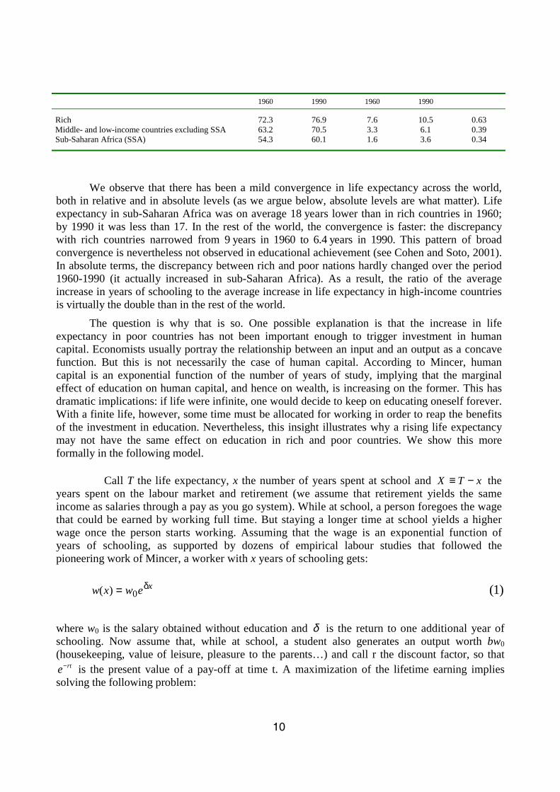
Table III.1. Life expectancy and education

Life Expectancyat age 5 (L5)

Average years ofschooling (YS)

∆YS/∆L5

!,

1960 1990 1960 1990

Rich 72.3 76.9 7.6 10.5 0.63Middle- and low-income countries excluding SSA 63.2 70.5 3.3 6.1 0.39Sub-Saharan Africa (SSA) 54.3 60.1 1.6 3.6 0.34

We observe that there has been a mild convergence in life expectancy across the world,both in relative and in absolute levels (as we argue below, absolute levels are what matter). Lifeexpectancy in sub-Saharan Africa was on average 18 years lower than in rich countries in 1960;by 1990 it was less than 17. In the rest of the world, the convergence is faster: the discrepancywith rich countries narrowed from 9 years in 1960 to 6.4 years in 1990. This pattern of broadconvergence is nevertheless not observed in educational achievement (see Cohen and Soto, 2001).In absolute terms, the discrepancy between rich and poor nations hardly changed over the period1960-1990 (it actually increased in sub-Saharan Africa). As a result, the ratio of the averageincrease in years of schooling to the average increase in life expectancy in high-income countriesis virtually the double than in the rest of the world.

The question is why that is so. One possible explanation is that the increase in lifeexpectancy in poor countries has not been important enough to trigger investment in humancapital. Economists usually portray the relationship between an input and an output as a concavefunction. But this is not necessarily the case of human capital. According to Mincer, humancapital is an exponential function of the number of years of study, implying that the marginaleffect of education on human capital, and hence on wealth, is increasing on the former. This hasdramatic implications: if life were infinite, one would decide to keep on educating oneself forever.With a finite life, however, some time must be allocated for working in order to reap the benefitsof the investment in education. Nevertheless, this insight illustrates why a rising life expectancymay not have the same effect on education in rich and poor countries. We show this moreformally in the following model.

Call T the life expectancy, x the number of years spent at school and xTX −≡ theyears spent on the labour market and retirement (we assume that retirement yields the sameincome as salaries through a pay as you go system). While at school, a person foregoes the wagethat could be earned by working full time. But staying a longer time at school yields a higherwage once the person starts working. Assuming that the wage is an exponential function ofyears of schooling, as supported by dozens of empirical labour studies that followed thepioneering work of Mincer, a worker with x years of schooling gets:

xewxw δ= 0)( (1)

where w0 is the salary obtained without education and δ is the return to one additional year ofschooling. Now assume that, while at school, a student also generates an output worth bw0

(housekeeping, value of leisure, pleasure to the parents…) and call r the discount factor, so thatrte− is the present value of a pay-off at time t. A maximization of the lifetime earning implies

solving the following problem:

!!

00

wdteedtebMaxx T

x

rtxrt

x

+∫ ∫ −δ− (2)

The first order condition is:

TXXr er

ber

e δ−δ−δ+−

δ+

δ−δ=)( (3)

This is the expression of an interior solution, which requires that 0>x or,equivalently, TX < . In the simple case when b = 0, this last condition is met if and only if:

δ−δ<− r

e rT

or,

mTr

Logr

T ≡

δ−−> 1

1

This means that if life expectancy is not long enough, a person would acquire no educationand spend all her life working. If b > 0, the threshold value of T required to investing a positivefraction of the time in education would be lower than Tm, since the opportunity cost of studyingwould be relatively low. By contrast, if b < 0, the minimum value of life expectancy needed tojustify some investing in education would be higher than Tm.

Let us now compute how the working time X varies with T. Deriving (3) with respect to T,we obtain,

TXXr breT

Xer

T

Xer δ−δ−δ+− +

∂∂−δ=

∂∂δ+ )()( )( .

Substituting ( )Xre δ+− by (3) and rearranging terms, we get:

( ) ( ) XT

T

ererb

be

T

Xδ−δ−

δ−

−δ+δ+δ=

∂∂

Then, recalling that xTX −≡ , we have:

( ) ( ) xerrb

b

T

Xδ−δ+δ+

δ=∂∂ (4)

!$

In the particular case when b=0, 0=∂∂

T

X (this can be deduced directly from (3)). This

means that any increase in life expectancy is channelled into education, provided that T is

sufficiently large. In the general case with b>0, T

X

∂∂

is positive but smaller than 1. This implies

that x increases with T, and so T

X

∂∂

is a decreasing function of T. Asymptotically, as T tends to

infinity, T

X

∂∂

tends towards zero, which means that any marginal increase of T is fully channelled

into education. So we have a non-linear relationship between life expectancy and education suchthat the marginal propensity to allocate time to education rises towards one. This is represented inFigure 1.

Figure 1. Incremental Schooling to Life Expectancy

T

dx/

dT

1

T*

There is a critical value T* below which life is entirely channelled into work life: noschooling takes place below that level. For small values of T > T* the level of education risesmildly with life expectancy. For large values of T, virtually any additional increase in lifeexpectancy is assigned to studying.

!%

IV. Empirical Estimates

This section analyses the empirical relationship between education and life expectancy. Themodel of section III predicts a positive relationship between these two variables, with a slopetending towards one. Figure 2 plots life expectancy at the age of 5 in 1990, against the averageyears of schooling of the population aged 25 to 29 in 2000. These are imperfect measures of thevariables implied by the model (the number of years of schooling planned life expectancy at themoment in which the planning is made). We use life expectancy at the age of 5 instead of themore commonly used measure of life expectancy at birth since it reflects better the time horizonfaced by a child at the moment she starts the formal education. Similarly, we prefer to use theaverage years of schooling of the population aged 25 to 29 in 2000 since it gauges better the finaleducational attainment of the generation under consideration%. The figure shows that for lowlevels of life expectancy the curve is almost flat, but as life expectancy increases the slopebecomes steeper. This is exactly what the model predicts.

Figure 2. Life Expectancy and Schooling

0

2

4

6

8

10

12

14

16

0 10 20 30 40 50 60 70 80 90Life expectancy at 5

(1990)

Yea

rs o

f sc

hoo

ling

(Pop

ula

tion

age

d 2

5-29

in 2

000)

"""""""""""""""""""""""""""""""""""""""""""3 It would be even better to use the years of schooling of population aged 25-29 in 2010 but we do not have thatinformation yet!

!&

Next, we proceed to the econometric estimation of the model. The model predicts thatschooling is a positive function of life expectancy, with an increasing slope. Table IV.3 presentsthe results for the estimation of the equation:

iti2

10-it210-it10it uL5L5YS +η+π+π+π= (4)

where YSit is years of schooling of population aged 25-29, L5it is life expectancy at age 5, ηi is acountry-specific effect and uit is a time-varying residual. The equation is estimated for t = 2000. Inmost of the regressions, life expectancy is highly significant. The OLS estimates of column 1suggest that, on average, countries reach a minimum level of education when life expectancy at 5is 55.3 years. To better illustrate these results, consider the case of Uganda. This country had in1990 one of the lowest levels of life expectancy at 5 (53.8 years) in the sample. Ten years later YSis estimated at 4.1, whereas the predicted value from column 1 is 3.9. The constrained estimates ofcolumn 2 — where the threshold for L5 yielding minimum education levels is fixed at 55 — donot vary substantially.

Table IV.3 Dependent Variable is Years of Schooling of Population 25-29 in 2000

OLS OLS GMM GMM(1) (2) (3) (4)

Observations 74 74 72 72Constant 50.3 50.49 59.95 62.28

(18.29) (3.46) (44.24) (12.19)L51990 −1.679 −1.873

(0.551) (1.323)(L51990)^2 1.52e-2 1.60e-2

(0.51e-2) (0.98e-2)L51990×(L51990 - C) 1.53e-2 1.65e-2

(0.13e-2) (0.38e-2)R2 0.672 0.672 0.647 0.647F-statistic (Prob. Value) <1% <1%Sargan (Prob. value) 95%

Note: Standard errors in parenthesis. Instruments for GMM are: constant, latitude, and lagged change of life5. C = 110in column (2) and 117.4 in column 4.

Yet, the OLS estimates are likely to have a positive bias since they do no account for thepresence of the country specific effect ηi. Arguably, ηi is correlated with L5it, hence the source ofinconsistency in OLS estimates. Column 3 reports the results obtained by GMM estimation. Inaddition to a constant, the instruments used are latitude and the 10-year change of L5it-10. Therationale for selecting the latitude of a country as an instrument is that countries with lowerlatitudes are prone to tropical diseases, an important factor determining life expectancy. At thesame time, it is hard to imagine that the latitude may have an impact on years of schooling otherthan through its effect on life expectancy. So latitude is likely to be a suitable instrument (this istested later).

The other instrument is L5i1990 - L5i1980. Taking life expectancy in differences removes thecountry-specific effect and so the source of endogeneity present in this variable disappears. Sincethe change in life expectancy is correlated with its level, changes are suitable instruments for

!'

levels. We also tried L5i1980 as an instrument, but its exogeneity was rejected by Sargan tests. Thisis a clear sign that country-specific effects are present in the dynamics of L5.

Column 3 presents unrestricted estimates of equation (4). As expected, the coefficients arelower than those obtained with OLS, and incidentally, they are not significant. In fact, the GMMestimation reported in column 3 is just identified (we use two instruments for two endogenousregressors), and so the estimation is inefficient. Column 4 presents the constrained version ofequation (4), where the threshold life expectancy is set at 54.85 years (this value is obtained fromcolumn 3). The constrained estimation reduces the number of regressors and makes possible anefficient estimation. As a result, the coefficient on L51990 is now highly significant. An F-test forthe first stage instrumental variable regression shows that the instruments used are alsosignificant. Finally, a Sargan test shows that the instruments are exogenous.

Using the parameters of column 4, we find that when life expectancy at 5 is worth 72.3(as in the average of high income countries in 1960), the equation predicts that 45 per cent of lifeimprovement will be channelled into schooling. When life expectancy is worth 63.2 (middle- andlow-income countries excluding in 1960) the number falls to 15 per cent. At the levels of lifeexpectancy of sub-Saharan Africa in 1960, virtually no education takes place (the average lifeexpectancy in sub-Saharan Africa has increased since then, which may explain the positive thoughmodest increase in schooling). These numbers understate the actual increase in the ∆YS/∆L5"ratioreported in Table III.1, but they are nevertheless consistent with the notion that schoolingattainment in countries with lower levels of life expectancy are less responsive to improvementsin the later.

V. THE LUCAS PARADOX

In order to analyse the Lucas paradox, it should first be emphasised that, in the Cobb-Douglas production function (1), it does not matter how one interprets itA (provided, as we

postulate, that there are no externalities). Depending on whether technical progress is Harrod,Solow or Hicks Neutral, the interpretation will differ on which remedies are called for in order toimprove productivity. Yet, the return to capital accumulation will always be simply driven by thederivative of output with respect to aggregate capital, i.e. as:

it

it

it

itit K

Q

K

Qr α=

∂∂

=

In the Cobb-Douglas case, as is well known, differences on the rate of return of capitalaccumulation are simply reflected in differences in average values of the output to capital ratio. Insuch a framework, the potential for capital mobility is huge as shown in Table V.1 below.

!(

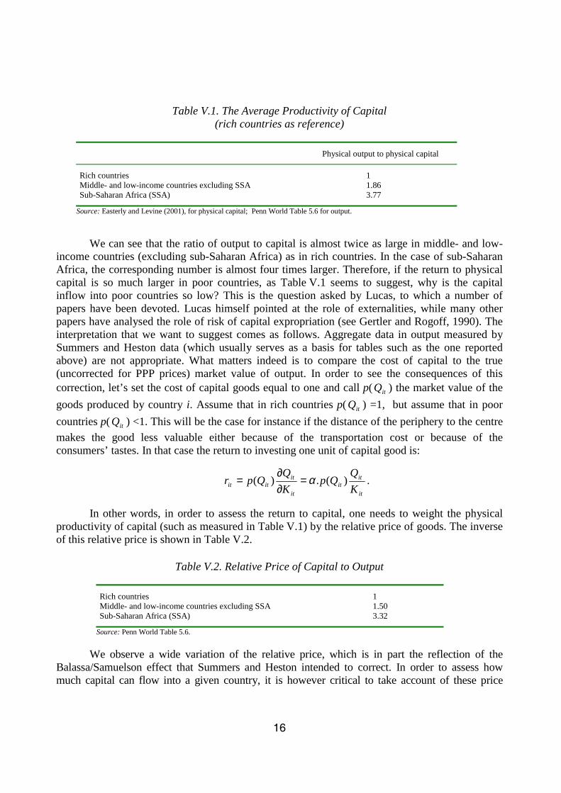
Table V.1. The Average Productivity of Capital(rich countries as reference)

Physical output to physical capital

Rich countries 1Middle- and low-income countries excluding SSA 1.86Sub-Saharan Africa (SSA) 3.77

Source: Easterly and Levine (2001), for physical capital; Penn World Table 5.6 for output.

We can see that the ratio of output to capital is almost twice as large in middle- and low-income countries (excluding sub-Saharan Africa) as in rich countries. In the case of sub-SaharanAfrica, the corresponding number is almost four times larger. Therefore, if the return to physicalcapital is so much larger in poor countries, as Table V.1 seems to suggest, why is the capitalinflow into poor countries so low? This is the question asked by Lucas, to which a number ofpapers have been devoted. Lucas himself pointed at the role of externalities, while many otherpapers have analysed the role of risk of capital expropriation (see Gertler and Rogoff, 1990). Theinterpretation that we want to suggest comes as follows. Aggregate data in output measured bySummers and Heston data (which usually serves as a basis for tables such as the one reportedabove) are not appropriate. What matters indeed is to compare the cost of capital to the true(uncorrected for PPP prices) market value of output. In order to see the consequences of thiscorrection, let’s set the cost of capital goods equal to one and call p( itQ ) the market value of the

goods produced by country i. Assume that in rich countries p( itQ ) =1, but assume that in poor

countries p( itQ ) <1. This will be the case for instance if the distance of the periphery to the centre

makes the good less valuable either because of the transportation cost or because of theconsumers’ tastes. In that case the return to investing one unit of capital good is:

it

itit

it

ititit K

QQp

K

QQpr )(.)( α=

∂∂

= .

In other words, in order to assess the return to capital, one needs to weight the physicalproductivity of capital (such as measured in Table V.1) by the relative price of goods. The inverseof this relative price is shown in Table V.2.

Table V.2. Relative Price of Capital to Output

Rich countries 1Middle- and low-income countries excluding SSA 1.50Sub-Saharan Africa (SSA) 3.32

Source: Penn World Table 5.6.

We observe a wide variation of the relative price, which is in part the reflection of theBalassa/Samuelson effect that Summers and Heston intended to correct. In order to assess howmuch capital can flow into a given country, it is however critical to take account of these price

!)

differences. This is done below, using the Easterly-Levine (2201) figure for physical capital, andcorrecting by the relative price of physical capital to output.

Table V.3. Relative Return to Capital

Rich countries 1Middle- and low-income countries excluding SSA 0.98Sub-Saharan Africa (SSA) 1.10

Note: Output per unit of capital, measured at market prices.

We see here that correcting by the relative price of capital wipes out the discrepancies inthe return to capital of Table V.1. Once the correction is made, the return to capital (measured asoutput per unit of capital, at market prices) is fairly equivalent in the three groups of countries.The ratio is marginally higher in sub-Saharan Africa, but it is well within the measurement errorof such type of exercise.

These results should clearly be interpreted with great caution. Many measurementproblems remain and the relative returns to capital of Table V.3 are constructed through themacroeconomics of the Cobb-Douglas production function, rather than through directmicroeconomic evidence. Direct evidence on the returns to foreign investment in sub-SaharanAfrica is reported in a number of papers. The overall picture is itself mixed. In Collier andGunning (1999), for instance, it is argued that the return on capital in sub-Saharan Africa up to theearly 1990s was on average about a third below the average of other emerging countries.Bhattacharya et al. (1996) report instead that returns on FDI are in the range of 24-32 per cent insub-Saharan Africa, while they are in the 16-18 per cent range for other developing countries. Butin a thought provoking paper based on macro data of Tanzania, Devarajan et al. (1999) argue thatsub-Saharan Africa’s low investment rate is due to its low return to capital. Collier and Patillo(2000) refer to all these points and argue quite convincingly that political risk is a majordeterminant of low investment in sub-Saharan Africa.

Yet, our interpretation on the apparent differences is not opposed to the existence ofpolitical risk. Furthermore, if our intuition is correct, we should find that when the analysis isrestricted to the manufacturing sector –which is essentially a tradable sector– we should notobserve the kind of capital shortage that we observe in macro PPP data (since the prices of goodsin the manufacturing sector are more less the same across countries). Using UNIDO data onmanufacturing, we computed capital output ratio across the world. We obtain the followingresults.

!*

Table IV.4. Capital- output ratio in the manufacturing sector(rich countries as reference)

Physical Capital to Physical Output

Rich countries 1Middle- and low-income countries excluding SSA 1.37Sub-Saharan Africa (SSA) 1.78

Source:UNIDO and author’s calculation.

This table shows that in poor countries there is no shortage of capital. In fact, we find thatthese countries have excess of capital as compared to the average of rich countries. This is exactlythe opposite of what we observe with aggregate PPP data and contradicts the Lucas Paradox.Overall, the fact that in the industrial sector we observe excess rather than lack of capital in poorcountries supports the view that PPP measures seriously distort the return of capital in aggregatedata.

VI. A comment on TFP

Before closing, it may be interesting to highlight in this section the simple fact that theefficient allocation of resources in a poor country is channelled towards the sector with a highlocal market price. Summers-Heston (SH) data, which are based on PPP prices, will necessarilypoint to a lower efficiency in poor countries simply because the allocation of resources in thosecountries will always appear to be sub-optimal since, to repeat, these are not the true prices underwhich countries operate. Imagine for instance that the economy consists of two sectors, one traded(say manufacturing) and one which is not traded internationally. Summers and Heston data assigna common relative price to these two sectors, the idea being that a hairdresser performs the sametask in New York and in Rio. Yet, if the market price of hairdressing is low, because the countryitself is poor, the return to investing physical capital in hairdressing will be low as well: thehairdressing sector will be capital-poor, and so will labour productivity. At SH prices, this will becounted as poor TFP, when it needs not be.

VII. Conclusion

Because non-traded activities are not valued at the price that they would receive in a richcountry, the profitability of capital is low, hence no investment takes place. This keeps theaggregate productivity of workers low. One implication of our analysis is to give support to the“transpiration” model pursued by Singapore (Young, 1995, and Krugman, 1994). Countries canbenefit more than is usually thought by simply raising human and physical capital stocks. Indeed,despite the huge differences in income across countries, a typical firm in a developing countrydoes not perform so badly compared to a firm in a rich country: it is not too far from the frontierof total productivity, nor is it too far from the level of human and physical capital either observed

!+

in rich countries. So, small progress in each of these items may lead the typical developingcountry substantially closer to the income level of rich countries. The message of hope is thatincreases in life expectancy may trigger economic development by pulling human capitalaccumulation and thus increasing the productivity of physical capital. The increased productivitycould eventually attract investment. By contrast, countries suffering from a deterioration of healthconditions will very likely, if not already, suffer from a serious decline of their income levels as aconsequence of the fall in human and physical accumulation.

$,

Appendix: countries used

Table A1

Rich countries Low- and middle-income countriesexcluding SSA

Sub-Saharan Africa (SSA)

Australia Algeria BeninAustria Argentina Burkina FasoBelgium Bangladesh BurundiCanada Bolivia CameroonCyprus Brazil Central African RepublicDenmark Chile GabonFinland China GhanaFrance Colombia Cote d'IvoireGreece Costa Rica KenyaIreland Dominican Republic MadagascarItaly Ecuador MalawiJapan Egypt, Arab Rep. MaliNetherlands El Salvador MauritiusNew Zealand Fiji NigeriaNorway Guatemala SenegalPortugal Guyana Sierra LeoneSingapore Honduras South AfricaSpain Hungary UgandaSweden India ZambiaSwitzerland Indonesia ZimbabweUnited Kingdom Iran, Islamic Rep.United States Jamaica

JordanKorea, Rep.MalaysiaMexicoMoroccoNicaraguaPanamaParaguayPeruPhilippinesSyrian Arab RepublicThailandTrinidad and TobagoTunisiaTurkeyUruguayVenezuela, RB

$!

Bibliography

ACEMOGLU, D. and F. ZILIBOTTI (2001), “Productivity Differences”, The Quarterly Journal of Economics, May,Vol. 116, pp. 563-606.

BHATTACHARYA, A, P. MONTIEL and S. SHARAM (1996), “Private Capital Flows to Sub-Saharan Africa”, ResearchDepartment, International Monetary Fund, Washington, D.C.

BILS, M. and P. KLENOW (2000), “Does Schooling Cause Growth?”, American Economic Review, (90)5, pp. 1160-83.

COE, D., E. HELPMAN and A. HOFFMAISTER (1997), “North-South R&D Spillovers”, Economic Journal, 107(440).

COHEN, D. (2002), “Fear of Globalization: The Human Capital Nexus”, Annual World Bank Conference onDevelopment Economics, pp. 69-93.

COHEN, D. and M. SOTO (2001), “Growth and Human Capital: Good Data, Good Results”, CEPR Working Paper,No. 3100, Centre for Economic Policy Research, London.

COLLIER, P. and J.W. GUNNING (1999) « Explaining African Economic Performance » Journal of EconomicLiterature, 37 (1), 64-111.

COLLIER, P. and C. PATILLO (eds.) (2000), Investment and Risk in Africa, Macmillan Press, London.

DEVARAJAN, S., W. EASTERLY and H. PACK (1999), “Is Investment in Africa Too High or Too Low? Macro andMicro Evidence”, World Bank, mimeo, Washington, D.C.

EASTERLY, W. (1999), “The Ghost of Financing Gap: Testing the Growth Model Used in the International FinancialInstitutions”, Journal of Development Economics, 60(2), December, pp. 423-38.

EASTERLY, W., M. KREMER, L. PRITCHETT and L. SUMMERS (1993), “Good Policies or Good Luck? CountryPerformances and Temporary Shocks”, Journal of Monetary Economics, 32(3), pp. 459-83.

EASTERLY, W. and R. LEVINE (2001), “It’s Not Factor Accumulation: Stylized Facts and Growth Models”, The WorldBank Economic Review, 15(2), pp. 177-219.

GERTLER, M. and K. ROGOFF (1990), “North South Lending and Endogenous Domestic Policies Inefficiencies”,Journal of Monetary Economics, 26, pp. 245-266.

HALL, R.E. and C.I. JONES (1999), “Why Do Some Countries Produce So Much More Output Per Worker ThanOthers?”, The Quarterly Journal of Economics, 114(1), pp. 83-116.

HECKMAN, J. and P. KLENOW (1997), “Human Capital Policy”, mimeo, University of Chicago.

KLENOW, P. and A. RODRIGUEZ-CLARE (1997), “The Neo-Classical Revival in Growth Economics: Has it Gone TooFar?”, NBER Macroeconomics Annual, National Bureau of Economic Research, Cambridge, Massachusetts.

KRUGMAN, P. (1994), “The Myth of Asia's Miracle”, Foreign Affairs, 73(6), Nov.-Dec., pp. 62-78.

KRUEGER, A. and M. LINDAHL (2001), “Education for Growth: Why and For Whom”, Journal of EconomicLiterature 39(4), 1101-1136.

LUCAS, R. (1988), “On the Mechanics of Economic Development”, Journal of Monetary Economics, 22, pp. 3-42.

MINCER, J. (1974), Schooling, Experience, and Earnings, Columbia University Press, New York.

SOTO, M. (2002), “Rediscovering Education”, TP 202, OECD Development Centre, Paris.

YOUNG, A. (1995), “The Tyranny of Numbers: Confronting the Statistical Realities of the East Asian GrowthExperience”, The Quarterly Journal of Economics, 110(3), pp. 641-680.

$$