WHT Marconi boards optimisation procedures

C.Jackman 10 May 2005Corrected: R. J. Pit, 24 Jul 2017

Setting up and adjusting the Marconi Analogue Processing Boards (APB)

Introduction

The function of the APB is to take analogue rate demands from either the counter board (CTB) or manual input controlson the engineering console and process these with angular velocity inputs from the tacho generators to provide stablecontrol of the telescope’s axes and other drives. With the exception of some TTL logic for controlling relays the signalprocessing on this board is wholly analogue. An APB is used to control the motion of each telescope drive (includingrotators) as well as the linear motion of the focus drive. Different moments of inertia (I) on each axis and the dynamicnature of azimuth axis (remember ‘I’ changes with telescope elevation) implies that each APB must be adjusted foroptimum performance on the telescope whilst controlling the intended load. There is little advantage therefore ofadjusting these boards off the telescope even if the necessary test fixtures were constructed, the only exception might beto isolate total failure of a component.

The range of loads APBs must accommodate means some fixed components must be selected before tuning the APBwith the intended load. It might also be necessary to select some components on test if the necessary adjustment cannotbe made using the range of the pot. It should be noted that this requirement has some bearing on the spares andmaintenance philosophy that can be adopted by the operations group. The best situation would be to have pre-tunedAPBs available as spares for each station. However, some relaxation ideal is possible without undue risk. In the author’sexperience nasmyth APBs can be interchanged without adjustment despite some possible difference in load, it should benoted that not all nasmyth loads are identical in any case e.g. changing between a derotator prism and Integral. Indesperate times other changes could be contemplated with care but an inappropriate board substituted in the azimuthposition is unlikely to operate at all telescope elevations.

Preparing and tuning an APB for a particular station

The component value table for all the APB's are listed in a seperate document which can be found hereThis procedure assumes that adjustments will be made on a board that either has not been used before or one that has anuncertain history. If an operational board is adjusted in an attempt to improve performance, but is subsequentlydiscovered to have components with different values to those indicated in the table, reasonable engineering judgementmust be exercised before substituting the ‘nominal’ value components the table.

Using the value table, configure an APB by inserting the appropriate fixed components for the particular station

Some Notes on differences between the first generation (old) APBoards, manufactured by Marconi,and the copies made RGO:

1. The circuitry around IC17, designed to introduce a test signal, has been elimanated on theRGO copies (new), and replaced by resistors and Switch 1.

2. R64 on the old boards has been renumbered R46 on the new boards. Resistor is in parallelwith R49.

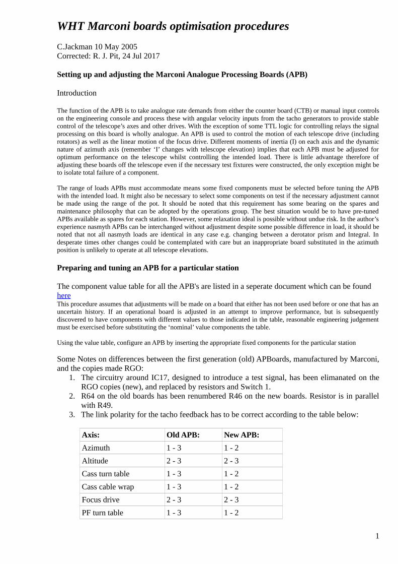
3. The link polarity for the tacho feedback has to be correct according to the table below:

Axis: Old APB: New APB:

Azimuth 1 - 3 1 - 2

Altitude 2 - 3 2 - 3

Cass turn table 1 - 3 1 - 2

Cass cable wrap 1 - 3 1 - 2

Focus drive 2 - 3 2 - 3

PF turn table 1 - 3 1 - 2

1

Nasmyth turn table 2 - 3 2 - 3

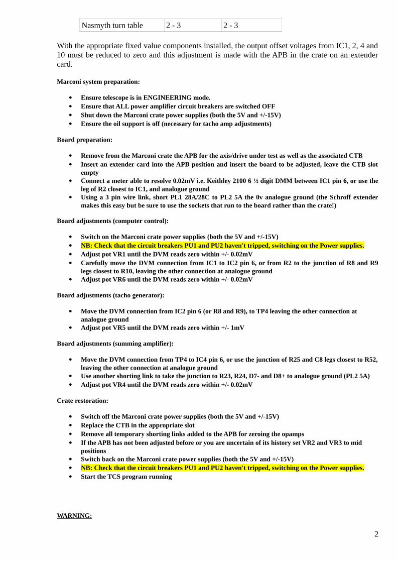
With the appropriate fixed value components installed, the output offset voltages from IC1, 2, 4 and10 must be reduced to zero and this adjustment is made with the APB in the crate on an extendercard.

Marconi system preparation:

Ensure telescope is in ENGINEERING mode. Ensure that ALL power amplifier circuit breakers are switched OFF Shut down the Marconi crate power supplies (both the 5V and +/-15V) Ensure the oil support is off (necessary for tacho amp adjustments)

Board preparation:

Remove from the Marconi crate the APB for the axis/drive under test as well as the associated CTB Insert an extender card into the APB position and insert the board to be adjusted, leave the CTB slot

empty Connect a meter able to resolve 0.02mV i.e. Keithley 2100 6 ½ digit DMM between IC1 pin 6, or use the

leg of R2 closest to IC1, and analogue ground Using a 3 pin wire link, short PL1 28A/28C to PL2 5A the 0v analogue ground (the Schroff extender

makes this easy but be sure to use the sockets that run to the board rather than the crate!)

Board adjustments (computer control):

Switch on the Marconi crate power supplies (both the 5V and +/-15V) NB: Check that the circuit breakers PU1 and PU2 haven't tripped, switching on the Power supplies. Adjust pot VR1 until the DVM reads zero within +/- 0.02mV Carefully move the DVM connection from IC1 to IC2 pin 6, or from R2 to the junction of R8 and R9

legs closest to R10, leaving the other connection at analogue ground Adjust pot VR6 until the DVM reads zero within +/- 0.02mV

Board adjustments (tacho generator):

Move the DVM connection from IC2 pin 6 (or R8 and R9), to TP4 leaving the other connection at analogue ground

Adjust pot VR5 until the DVM reads zero within +/- 1mV

Board adjustments (summing amplifier):

Move the DVM connection from TP4 to IC4 pin 6, or use the junction of R25 and C8 legs closest to R52,leaving the other connection at analogue ground

Use another shorting link to take the junction to R23, R24, D7- and D8+ to analogue ground (PL2 5A) Adjust pot VR4 until the DVM reads zero within +/- 0.02mV

Crate restoration:

Switch off the Marconi crate power supplies (both the 5V and +/-15V) Replace the CTB in the appropriate slot Remove all temporary shorting links added to the APB for zeroing the opamps If the APB has not been adjusted before or you are uncertain of its history set VR2 and VR3 to mid

positions Switch back on the Marconi crate power supplies (both the 5V and +/-15V) NB: Check that the circuit breakers PU1 and PU2 haven't tripped, switching on the Power supplies. Start the TCS program running

WARNING:

2

During the subsequent parts of this set-up procedure the telescope drive being adjusted may oscillate or run outof control. It is important to ensure all personnel not involved with this activity are aware what may happen andare not close to moving machinery (nasmyth or prime rotators) or moving structures (altitude, azimuth axes orcassegrain rotator).

It is also important to be aware of the way the drive is behaving, and be in a position to use the emergency stopsor other controls to quickly bring the system to the previously stable state (i.e. switching back to engineering).

In the early stages of adjustment it is not a good idea to have more power amplifiers on than are necessary forthe test. Only when it is reasonably certain the drive being adjusted is stable should other drives be powered andslewing and tracking scenarios sent from the TCS.

Testing with manual control:

Switch on the appropriate power amplifiers for the test Check that the drive being adjusted is not oscillating or drifting Turn the manual demand control to minimum (altitude and azimuth) Using the buttons and manual rate controls check that the drive can be moved in either direction. It

should be noted that when performing this test on the azimuth or altitude axis it is very easy to trip the circuit breakers at the bottom of the Marconi rack by applying excessive acceleration. This should not necessarily be taken as indicating abnormal performance, simply that more care is needed when increasing the demand

If the drive drifts away without any demand try increasing the tacho feedback, increase VR3

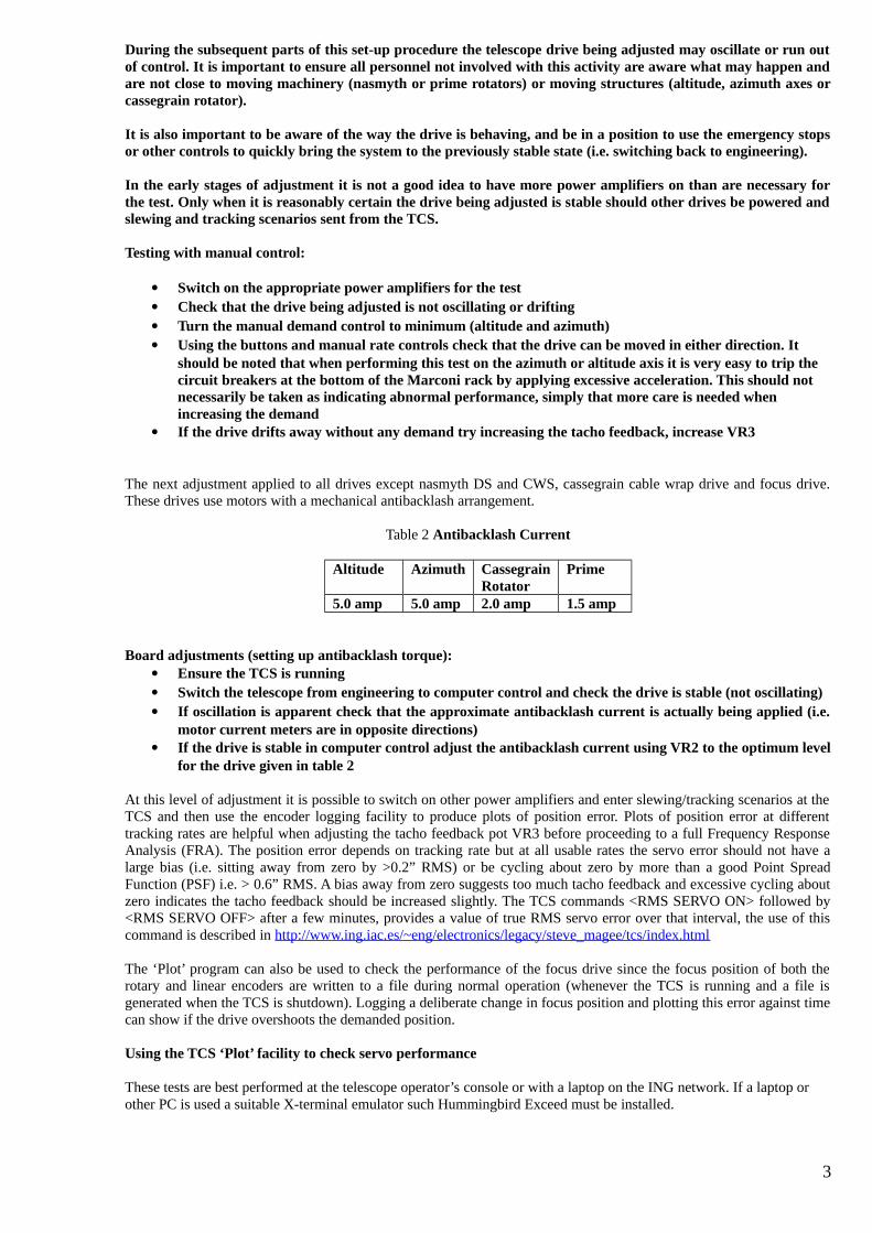
The next adjustment applied to all drives except nasmyth DS and CWS, cassegrain cable wrap drive and focus drive.These drives use motors with a mechanical antibacklash arrangement.

Table 2 Antibacklash Current

Altitude Azimuth CassegrainRotator

Prime

5.0 amp 5.0 amp 2.0 amp 1.5 amp

Board adjustments (setting up antibacklash torque): Ensure the TCS is running Switch the telescope from engineering to computer control and check the drive is stable (not oscillating) If oscillation is apparent check that the approximate antibacklash current is actually being applied (i.e.

motor current meters are in opposite directions) If the drive is stable in computer control adjust the antibacklash current using VR2 to the optimum level

for the drive given in table 2

At this level of adjustment it is possible to switch on other power amplifiers and enter slewing/tracking scenarios at theTCS and then use the encoder logging facility to produce plots of position error. Plots of position error at differenttracking rates are helpful when adjusting the tacho feedback pot VR3 before proceeding to a full Frequency ResponseAnalysis (FRA). The position error depends on tracking rate but at all usable rates the servo error should not have alarge bias (i.e. sitting away from zero by >0.2” RMS) or be cycling about zero by more than a good Point SpreadFunction (PSF) i.e. > 0.6” RMS. A bias away from zero suggests too much tacho feedback and excessive cycling aboutzero indicates the tacho feedback should be increased slightly. The TCS commands <RMS SERVO ON> followed by<RMS SERVO OFF> after a few minutes, provides a value of true RMS servo error over that interval, the use of thiscommand is described in http://www.ing.iac.es/~eng/electronics/legacy/steve_magee/tcs/index.html

The ‘Plot’ program can also be used to check the performance of the focus drive since the focus position of both therotary and linear encoders are written to a file during normal operation (whenever the TCS is running and a file isgenerated when the TCS is shutdown). Logging a deliberate change in focus position and plotting this error against timecan show if the drive overshoots the demanded position.

Using the TCS ‘Plot’ facility to check servo performance

These tests are best performed at the telescope operator’s console or with a laptop on the ING network. If a laptop or other PC is used a suitable X-terminal emulator such Hummingbird Exceed must be installed.

3

Generating an encoder file: -

Once the telescope is tracking steadily, type the command <log enc on> and accept the 15 min default After 2 min terminate the logging by typing <log enc off> and note the name of the file generated (e.g.

DISK$LOGS: [WHT.DATA.ENCODER]enc050507.dat;1)

From the TO console:

Using the ‘terminal’ pull down menu establish a new LAT session with LPAS4 Either of two accounts can be used for running PLOT, genuser or tcsmgr, the former is a captive account

that can only be used for PLOT and another program called PAIRS. The latter is less restrictive and better if data needs to be exported to a PC to be analysed with other applications such as Excel or Matlab

Enter the appropriate password

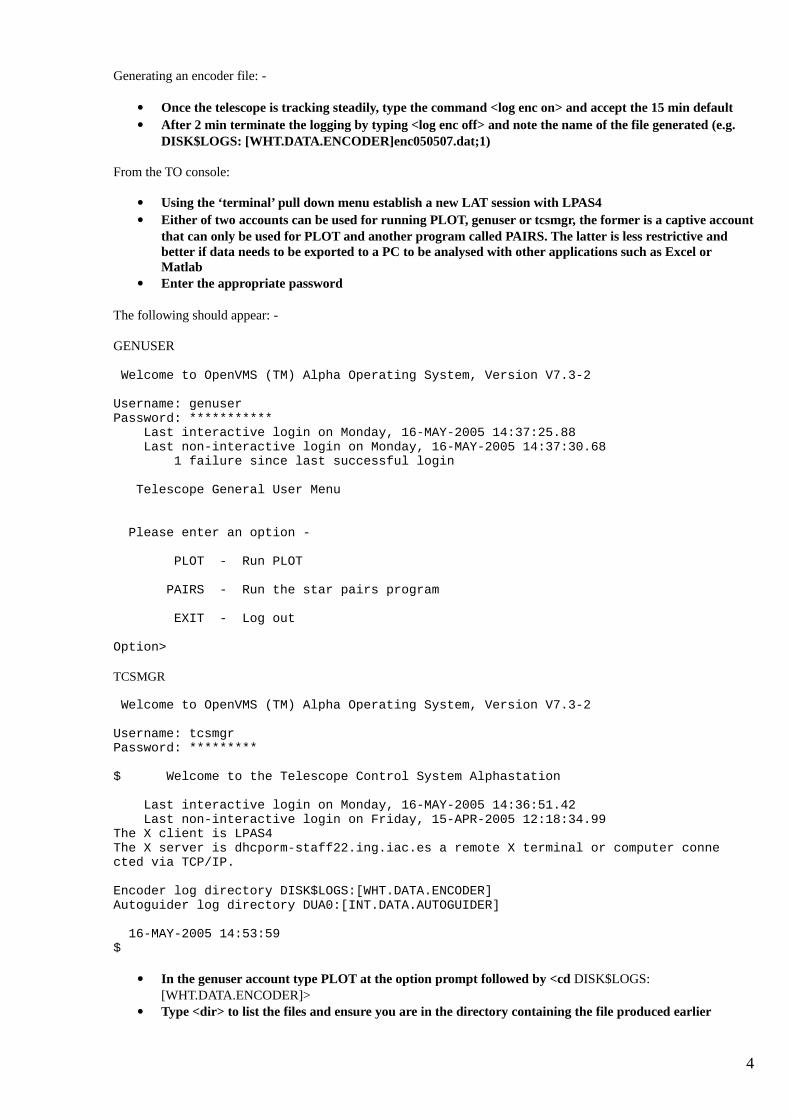
The following should appear: -

GENUSER

Welcome to OpenVMS (TM) Alpha Operating System, Version V7.3-2

Username: genuserPassword: *********** Last interactive login on Monday, 16-MAY-2005 14:37:25.88 Last non-interactive login on Monday, 16-MAY-2005 14:37:30.68 1 failure since last successful login

Telescope General User Menu

Please enter an option -

PLOT - Run PLOT

PAIRS - Run the star pairs program

EXIT - Log out

Option>

TCSMGR

Welcome to OpenVMS (TM) Alpha Operating System, Version V7.3-2

Username: tcsmgrPassword: *********

$ Welcome to the Telescope Control System Alphastation

Last interactive login on Monday, 16-MAY-2005 14:36:51.42 Last non-interactive login on Friday, 15-APR-2005 12:18:34.99The X client is LPAS4The X server is dhcporm-staff22.ing.iac.es a remote X terminal or computer connected via TCP/IP.

Encoder log directory DISK$LOGS:[WHT.DATA.ENCODER]Autoguider log directory DUA0:[INT.DATA.AUTOGUIDER]

16-MAY-2005 14:53:59$

In the genuser account type PLOT at the option prompt followed by <cd DISK$LOGS:[WHT.DATA.ENCODER]>

Type <dir> to list the files and ensure you are in the directory containing the file produced earlier

4

In the tcsmgr account it is a good practice to first change to the DISK$LOGS:[WHT.DATA.ENCODER] directory by typing <set def DISK$LOGS:[WHT.DATA.ENCODER]> before starting the program by typing PLOT at the $ prompt. Instructions that follow are the same in either account from the PLOT> prompt. At the prompt it is always possible to <help> and list the available commands with definitions and examples.

To plot the file in the example enc050507.dat;1

At the PLOT> prompt, type <data enc050507.dat;1> and a record of available variables that can be plotted is listed.

PLOT>data enc050412.dat;1WHT 20050412Encoder log fileNumber of data fields = 32

Key 1 Key 2 Label

UTC TimeAZIMUTH ABS Azimuth AbsoluteAZIMUTH GEAR Azimuth GearAZIMUTH ROLL Azimuth RollerAZIMUTH TAPE1 Azimuth Tape 1AZIMUTH TAPE2 Azimuth Tape 2AZIMUTH TAPE3 Azimuth Tape 3AZIMUTH TAPE4 Azimuth Tape 4ALTITUDE ABS Elevation AbsoluteALTITUDE GEAR Elevation GearALTITUDE ROLL Elevation RollerFOCUS ABS Focus AbsoluteDOME ABS Dome AbsoluteAZIMUTH POSERR Azimuth pos errorALTITUDE POSERR Altitude pos errorCASS POSERR Cassegrain pos errorFOCUS POSERR Focus pos errorDOME POSERR Dome pos errorAZIMUTH VEL_DEM Azimuth demandALTITUDE VEL_DEM Altitude demandCASS VEL_DEM Cassegrain demandDOME VEL_DEM Dome demandFOCUS VEL_DEM Focus demandCASS ABS Cassegrain AbsoluteCASS INC Cass Incremental HORDIS1 Horiz Displacement 1 HORDIS2 Horiz Displacement 2 SECPOS1 Secondary Position 1 SECPOS2 Secondary Position 2 SECPOS3 Secondary Position 3 AZMOTOR1 Az Drive Motor 1 AZMOTOR2 Az Drive Motor 2 1200 records in the data filePLOT>

When tuning APBs rather than investigating suspected telescope faults or poor tracking reports, plotting one of the fourPOSERR parameters against UTC are the most useful.

Type <read 1 UTC> to plot time along the x-axis Type <read 2 AZIMUTH POSERR> to plot azimuth position error up the y-axis Type <dev xwin> to define the plotting device as an xterminal window, there are other plotting options

such as PS printers use <help> and <device> to see what is available Type <lim> to set plotting limits Type <plot> to plot the graph in an xwindow in this example

An APB set up correctly should have a trace that appears symmetrical about zero and only cycles through zero with asmall amplitude. Fig1 is an example of azimuth tracking with a large (-1.28”) offset suggesting that the tacho feedbackshould be decreased. Fig2 illustrates good tracking, the servo error trace is symmetrical about zero and the RMSamplitude is much smaller than a typical PSF in fact even the highest peaks are between ~-0.2” and 0.2”. Even with a

5

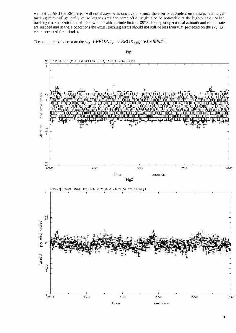
well set up APB the RMS error will not always be as small as this since the error is dependent on tracking rate, largertracking rates will generally cause larger errors and some offset might also be noticeable at the highest rates. Whentracking close to zenith but still below the usable altitude limit of 89 o.8 the largest operational azimuth and rotator rateare reached and in these conditions the actual tracking errors should not still be less than 0.3” projected on the sky (i.e.when corrected for altitude).

The actual tracking error on the sky ERRORSKY=ERRORRMS cos( Altitude)

Fig1

Fig2

6

This procedure is intended to be sufficient when preparing a new APB board for use as an operational spare. If thesubstituted board will remain in place after the faulty board is repaired then it is advisable to perform frequencyresponse measurements on the drive and compare the results with previous measurements made with the original board.This ensures that the dominant resonant frequencies have not changed significantly as a result of the board substitution.It should also be remembered that any major changes to the rotating mass of the telescope might also alter the torsionalresonance. The procedure for taking and analysing these measurements is given in detail in a document by MartinFisher “WHT visit report May 2003_appendices”. The part of the report describing the use of both the Solartrontransfer function analyser and Siglab for making FRA measurements has been extracted and added as an appendix tothis document.

Appendix 1

Frequency Response Analysis Measurements

Principle of measurement:

The purpose of measuring a system’s Transfer Function (TF) is to determine its stability and optimise its performance.Measurements could be made open loop in order to determine the response in closed loop but this is not necessary whenit is known that the closed loop system is stable. In fact it is more convenient to make closed loop measurements andplot them on the closed loop coordinates of the Nicholls chart. This is valid if the system is of second order or thedominant poles of the transfer function are sufficiently 'dominant'. It is then easy to estimate the compensationnecessary to optimise the response. The general method for obtaining frequency response measurements using a TFanalyser is to inject a disturbance signal, usually a sine wave, at a summing junction at some point in the circuit andthen to measure the response at some point, usually just before the injection. The amplitude and phase of the injectedand feedback signals are then compared or correlated to produce a transfer function. Usually the average of a number ofmeasurements is made in order to improve the coherence.

Equipment needed:SiglaborSolartron 1250 Transfer Function Analyser ( TFA ) plus an Oscilloscope and optionally a PC or printer with serial I/F.The setting up instructions for the Solartron FRA are shown below in detail.Solartron System

Setting up:The generator output of the TFA is connected to the injection point through a suitable resistor so as to preserve unityscaling of output/input signals. The generator output is also connected to channel l of the analyser section while thefeedback signal is input to channel 2. Thus the analyser can be set to provide direct results by choosing to measureCh2/Chl. In order that non-linearities do not interfere with the measurement it is usual to bias the motion of thetelescope with a constant offset demand and then modulate this with a signal whose amplitude does not exceed the bias.There are a number of ways of doing this but the preferred methods depend on the measurement to be performed andare described below.

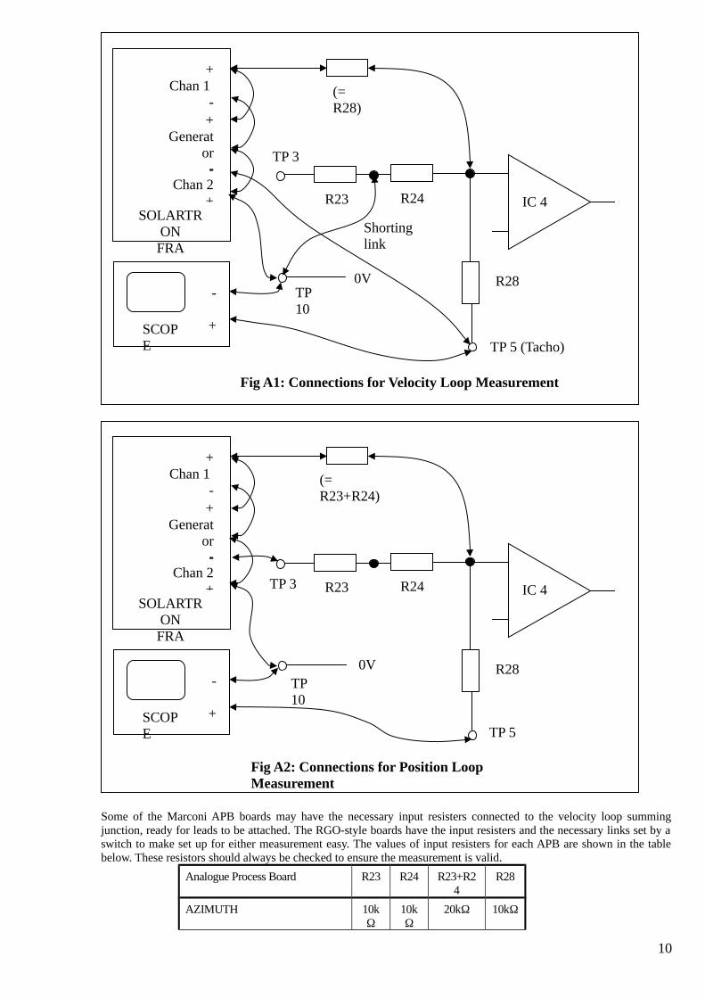
Measurement of closed position loop:Connections for this are shown in Fig A1. The TFA generator output is connected to the summing junction of thevelocity loop at IC4 through a resistor equal to the sum of the resistors that connect the integrated position error to thesame point. This ensures unity gain between the injected disturbance signal and the measured response at TP3, which isthe position error. If this is not done then the change in gain must be taken into account. The generator signal is alsoconnected to channel 1 and the response is connected to channel 2 so that the complex ratio of Ch2/Chl gives the systemresponse directly. Note that the Ch2 inputs are inverted. This is because of the negative feedback connection of theposition loop and in order to display the correct phase relationship it is necessary to re-invert the response signal. Ascope is connected to the tacho signal in order to monitor the behaviour of the drive and ensure that the drive does notreverse or saturate on application of the disturbance signal. For this test the bias is applied via the control computersince any bias applied by the generator would be counteracted by action of the closed loop servo trying to maintainposition - a battle which bias cannot win! It is also necessary that the T/S is operating in computer mode so that anti-backlash torque is applied.The drive can be set up to slew at a constant low velocity by changing the software velocity limit to a suitably low valueand then commanding a slew to a position far enough away to allow time for the measurement to be made. The changeto the velocity limit is made in the TCS using the Global Section editor "gsexam" and the procedure described later.With the drive slewing slowly the stimulus or disturbance can be applied in small increments until a desirable level is

7

reached. Note that the response will vary with frequency and a check must be made at each measurement to ensure thebias is not being overcome by a high signal level or that the response is so low as to cause coherence problems for theanalyser. A suitable integration time should be chosen such that results are consistent. This depends on the S/N of theresponse and the linearity of the system under test. On the WHT integration over 10 cycles has been adequate. On theINT an integration of l00 cycles may be required although this is tedious at 0.1 Hz!Warning: care must be taken not to over-excite the system under test as this can cause damage let alone producemeaningless results. The stimulus should be kept small. Care with entering the amplitude and frequencyparameters is needed and a close watch kept on the tacho voltage signal on the oscilloscope so as to avoidproblems with resonances of the system.

Connections for velocity loop measurement:In this case signal injection is at the same point but via a resistor of the same value as the tacho feedback resistor fromTP5 (R28). The response signal is measured at the (TP5) and again the Ch2 connections are reversed. For this test, theposition loop must be disabled for the measurements to be valid otherwise the position loop fights the velocity loop.The position loop is disabled without disabling the anti-backlash current by shorting the position error signal at thejunction of R23 and R24 to ground. The velocity bias can now be applied using the TFA and increased until anappropriate rate is indicated by the tacho output. The system is still in computer mode for the test even though theposition loop is disabled. All the precautions mentioned above are still applicable.

8

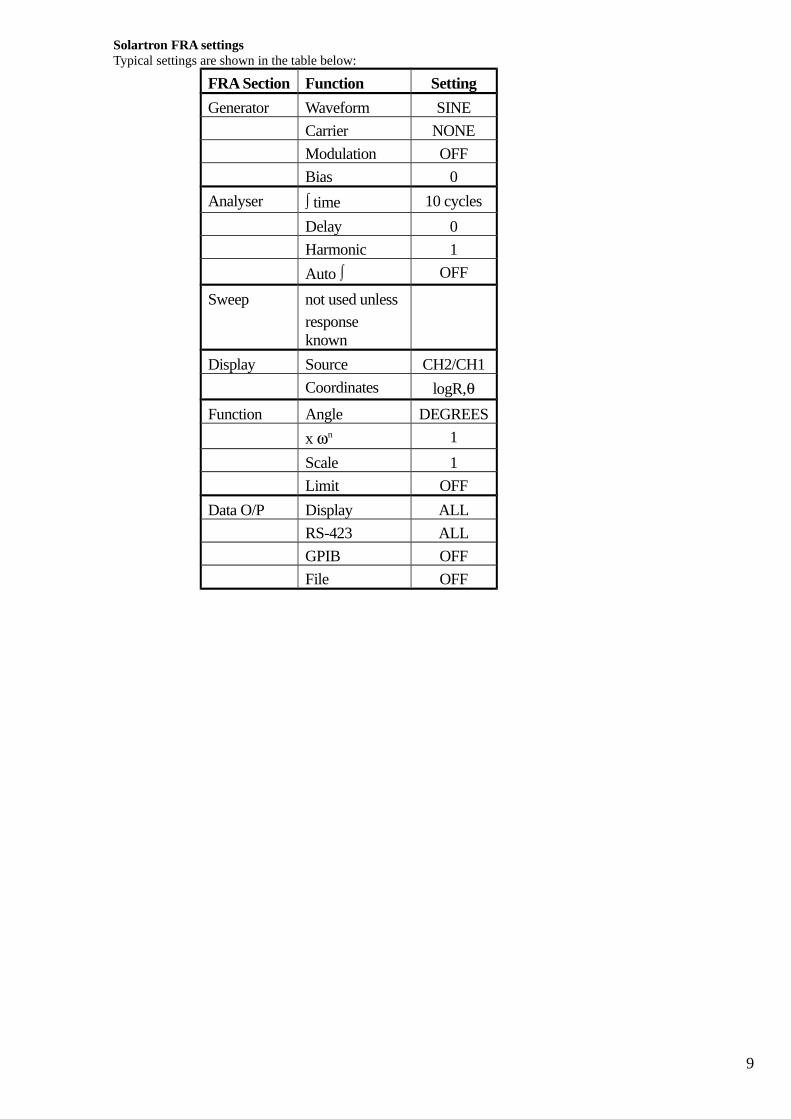
Solartron FRA settingsTypical settings are shown in the table below:

FRA Section Function Setting

Generator Waveform SINE

Carrier NONE

Modulation OFF

Bias 0

Analyser time 10 cycles

Delay 0

Harmonic 1

Auto OFF

Sweep not used unless

response known

Display Source CH2/CH1

Coordinates logR,Function Angle DEGREES

x n 1

Scale 1

Limit OFF

Data O/P Display ALL

RS-423 ALL

GPIB OFF

File OFF

9

Some of the Marconi APB boards may have the necessary input resisters connected to the velocity loop summingjunction, ready for leads to be attached. The RGO-style boards have the input resisters and the necessary links set by aswitch to make set up for either measurement easy. The values of input resisters for each APB are shown in the tablebelow. These resistors should always be checked to ensure the measurement is valid.

Analogue Process Board R23 R24 R23+R24

R28

AZIMUTH 10kΩ

10kΩ

20kΩ 10kΩ

10

+Chan 1

-

-Chan 2

+

+Generat

or-

SOLARTRONFRA

-

+

IC 4

(= R23+R24)

R23 R24

R280V

SCOPE TP 5

TP 3

TP 10

Fig A2: Connections for Position Loop Measurement

Shorting link

+Chan 1

-

-Chan 2

+

+Generat

or-

SOLARTRONFRA

-

+

IC 4

(= R28)

R23 R24

R280V

SCOPE TP 5 (Tacho)

TP 3

TP 10

Fig A1: Connections for Velocity Loop Measurement

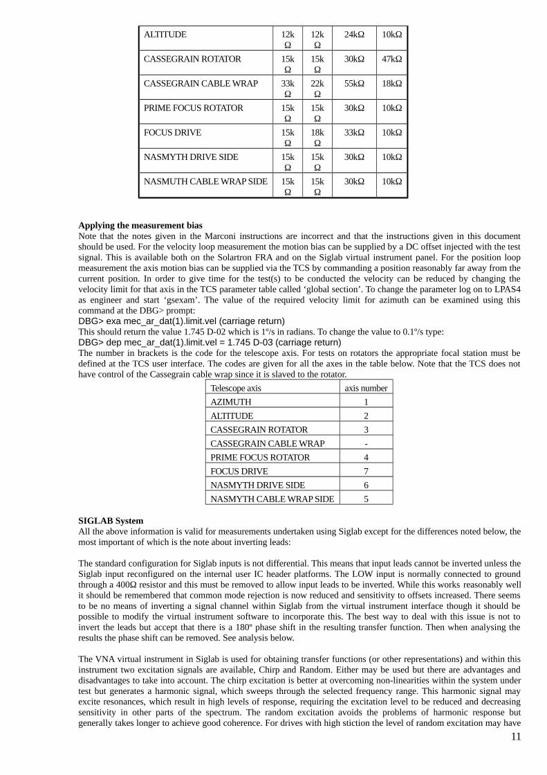
ALTITUDE 12kΩ

12kΩ

24kΩ 10kΩ

CASSEGRAIN ROTATOR 15kΩ

15kΩ

30kΩ 47kΩ

CASSEGRAIN CABLE WRAP 33kΩ

22kΩ

55kΩ 18kΩ

PRIME FOCUS ROTATOR 15kΩ

15kΩ

30kΩ 10kΩ

FOCUS DRIVE 15kΩ

18kΩ

33kΩ 10kΩ

NASMYTH DRIVE SIDE 15kΩ

15kΩ

30kΩ 10kΩ

NASMUTH CABLE WRAP SIDE 15kΩ

15kΩ

30kΩ 10kΩ

Applying the measurement biasNote that the notes given in the Marconi instructions are incorrect and that the instructions given in this documentshould be used. For the velocity loop measurement the motion bias can be supplied by a DC offset injected with the testsignal. This is available both on the Solartron FRA and on the Siglab virtual instrument panel. For the position loopmeasurement the axis motion bias can be supplied via the TCS by commanding a position reasonably far away from thecurrent position. In order to give time for the test(s) to be conducted the velocity can be reduced by changing thevelocity limit for that axis in the TCS parameter table called ‘global section’. To change the parameter log on to LPAS4as engineer and start ‘gsexam’. The value of the required velocity limit for azimuth can be examined using thiscommand at the DBG> prompt:DBG> exa mec_ar_dat(1).limit.vel (carriage return)This should return the value 1.745 D-02 which is 1º/s in radians. To change the value to 0.1º/s type:DBG> dep mec_ar_dat(1).limit.vel = 1.745 D-03 (carriage return)The number in brackets is the code for the telescope axis. For tests on rotators the appropriate focal station must bedefined at the TCS user interface. The codes are given for all the axes in the table below. Note that the TCS does nothave control of the Cassegrain cable wrap since it is slaved to the rotator.

Telescope axis axis number

AZIMUTH 1

ALTITUDE 2

CASSEGRAIN ROTATOR 3

CASSEGRAIN CABLE WRAP -

PRIME FOCUS ROTATOR 4

FOCUS DRIVE 7

NASMYTH DRIVE SIDE 6

NASMYTH CABLE WRAP SIDE 5

SIGLAB SystemAll the above information is valid for measurements undertaken using Siglab except for the differences noted below, themost important of which is the note about inverting leads:

The standard configuration for Siglab inputs is not differential. This means that input leads cannot be inverted unless theSiglab input reconfigured on the internal user IC header platforms. The LOW input is normally connected to groundthrough a 400Ω resistor and this must be removed to allow input leads to be inverted. While this works reasonably wellit should be remembered that common mode rejection is now reduced and sensitivity to offsets increased. There seemsto be no means of inverting a signal channel within Siglab from the virtual instrument interface though it should bepossible to modify the virtual instrument software to incorporate this. The best way to deal with this issue is not toinvert the leads but accept that there is a 180º phase shift in the resulting transfer function. Then when analysing theresults the phase shift can be removed. See analysis below.

The VNA virtual instrument in Siglab is used for obtaining transfer functions (or other representations) and within thisinstrument two excitation signals are available, Chirp and Random. Either may be used but there are advantages anddisadvantages to take into account. The chirp excitation is better at overcoming non-linearities within the system undertest but generates a harmonic signal, which sweeps through the selected frequency range. This harmonic signal mayexcite resonances, which result in high levels of response, requiring the excitation level to be reduced and decreasingsensitivity in other parts of the spectrum. The random excitation avoids the problems of harmonic response butgenerally takes longer to achieve good coherence. For drives with high stiction the level of random excitation may have

11

to be high to get a consistent response in which case harmonic excitation is likely to be the better option. Both methodsshould be tried unless the preferred method has already been established.

SIGLAB analysisOnce a Siglab test has been completed it should be saved to a .vna file but also exported to a text file by selecting‘export’ and ‘transfer function’. The text file contains headers, which describe the instrument setup and so are useful butmay get in the way when importing them to Matlab. One way to deal with this is to edit the text file by placing a ‘%’ atthe start of each line to be ignored by Matlab. Some data lines at the start of the measurement also may need to beexcluded because they contain spurious measurements at very low frequency. With the file in Matlab workspace theresponse can then be plotted as desired. To automate this process an m-file has been developed which loads the editedtext file, allows the user to apply gain or phase modifications and prepares the data for plotting within the LTI viewer. Itdoes this by converting the frequency response data into complex form, applying the inverse Nichols function toconvert the closed loop response to an open loop response and then taking both these responses and converting them toa system so that it can be imported as such into the LTI viewer or directly plotted using standard control system toolboxplot commands. The m-file is called clo2op.m and is shown below. The script does not produce plots but prepares thedata for plotting. It also includes a function for interpolating between data points which is useful when only a few pointsare available so in general one should use olsys as the import or plot data and only use iolsys if required. The Nicholsplot requires open loop frequency response data since it uses those coordinates in its plot routine. The open and closedloop data is useful for Bode plots.Typical set up appearance for the Siglab VNA instrument is also shown below in examples of both chirp and randomexcitation performed on the azimuth axis of the WHT for tube vertical and tube at 45º zenith distance. The instrumentsetup window is shown together with the resulting frequency response window for each case. Note the similarity of theresponse for chirp and random excitation but also the noisier high frequency response using chirp. Note also thedifferent response between different tube elevations.

12

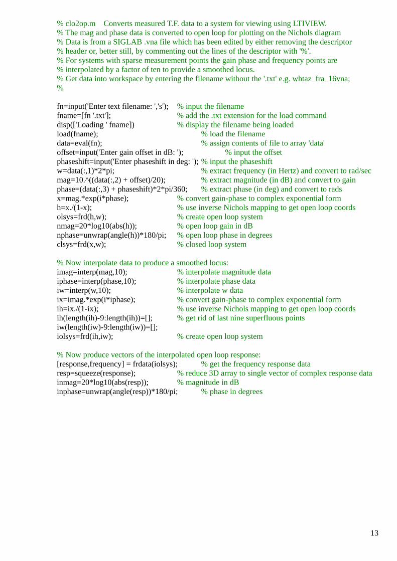
% clo2op.m Converts measured T.F. data to a system for viewing using LTIVIEW.% The mag and phase data is converted to open loop for plotting on the Nichols diagram% Data is from a SIGLAB .vna file which has been edited by either removing the descriptor% header or, better still, by commenting out the lines of the descriptor with '%'.% For systems with sparse measurement points the gain phase and frequency points are % interpolated by a factor of ten to provide a smoothed locus.% Get data into workspace by entering the filename without the '.txt' e.g. whtaz_fra_16vna;%

fn=input('Enter text filename: ','s'); % input the filenamefname=[fn '.txt']; % add the .txt extension for the load commanddisp(['Loading ' fname]) % display the filename being loadedload(fname); % load the filenamedata=eval(fn); % assign contents of file to array 'data'offset=input('Enter gain offset in dB: '); % input the offsetphaseshift=input('Enter phaseshift in deg: '); % input the phaseshiftw=data(:,1)*2*pi; % extract frequency (in Hertz) and convert to rad/secmag=10.^((data(:,2) + offset)/20); % extract magnitude (in dB) and convert to gainphase=(data(:,3) + phaseshift)*2*pi/360; % extract phase (in deg) and convert to radsx=mag.*exp(i*phase); % convert gain-phase to complex exponential formh=x./(1-x); % use inverse Nichols mapping to get open loop coordsolsys=frd(h,w); % create open loop systemnmag=20*log10(abs(h)); % open loop gain in dBnphase=unwrap(angle(h))*180/pi; % open loop phase in degreesclsys=frd(x,w); % closed loop system

% Now interpolate data to produce a smoothed locus:imag=interp(mag,10); % interpolate magnitude dataiphase=interp(phase,10); % interpolate phase dataiw=interp(w,10); % interpolate w dataix=imag.*exp(i*iphase); % convert gain-phase to complex exponential formih=ix./(1-ix); % use inverse Nichols mapping to get open loop coordsih(length(ih)-9:length(ih))=[]; % get rid of last nine superfluous pointsiw(length(iw)-9:length(iw))=[];iolsys=frd(ih,iw); % create open loop system

% Now produce vectors of the interpolated open loop response:[response,frequency] = frdata(iolsys); % get the frequency response dataresp=squeeze(response); % reduce 3D array to single vector of complex response datainmag=20*log10(abs(resp)); % magnitude in dBinphase=unwrap(angle(resp))*180/pi; % phase in degrees

13

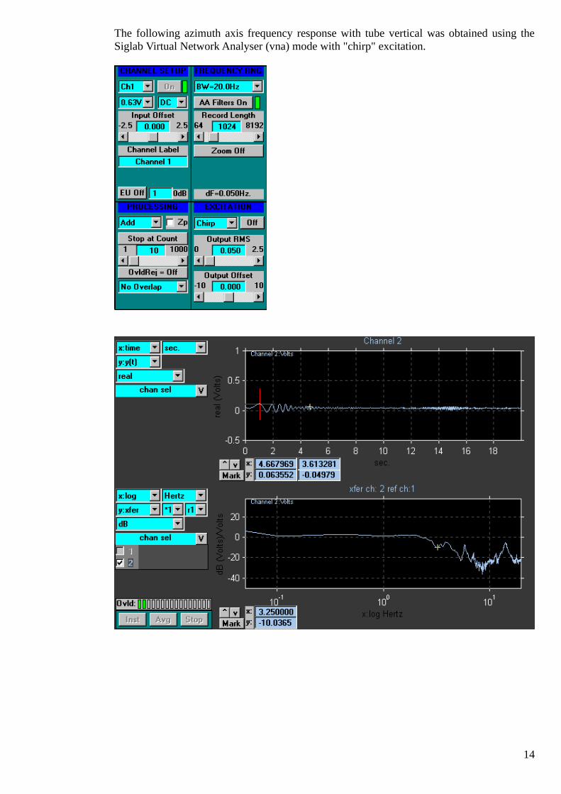
The following azimuth axis frequency response with tube vertical was obtained using theSiglab Virtual Network Analyser (vna) mode with "chirp" excitation.

14

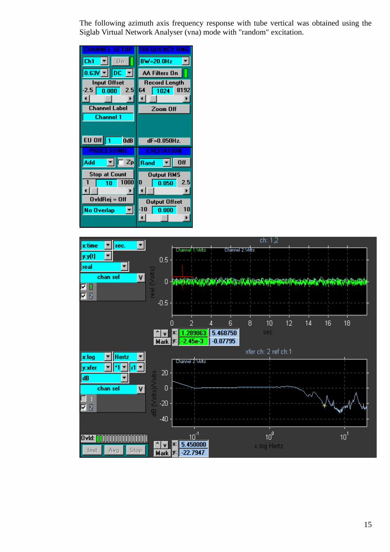
The following azimuth axis frequency response with tube vertical was obtained using theSiglab Virtual Network Analyser (vna) mode with "random" excitation.

15

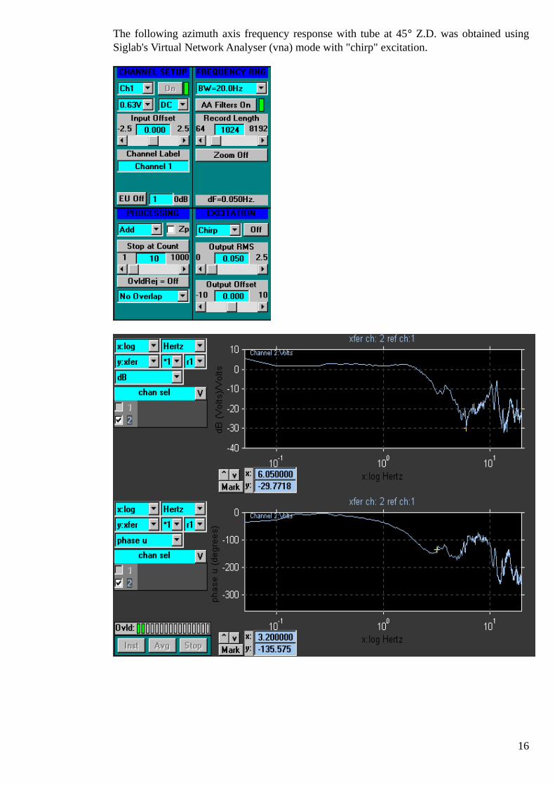
The following azimuth axis frequency response with tube at 45 Z.D. was obtained usingSiglab's Virtual Network Analyser (vna) mode with "chirp" excitation.

16

Tuning:Should this ever need to be re-done then the basic points are covered below. It is not a procedure that can beautomatically followed, one has to understand both the theory and practice of control systems to be able to analyse andassess the system under test and be on the lookout for indications of problems which are not of a tuning nature e.g. non-linearities, regular disturbances such as torque ripple or significant high-order terms which should not be ignored.

The Marconi system is a nested loop control system. The velocity loop should be tuned first to give good response overa wide bandwidth. The higher the loop gain and bandwidth in the velocity loop the better will be the disturbancerejection provided there is no saturation introduced in the loop. However this loop will affect the characteristics of theouter rate or digital loop and too much gain will cause problems for stability. Increasing the velocity loop gain willintroduce phase lead into the rate or position loop but also increase the high frequency gain. A compromise needs to befound which provides the best disturbance rejection properties with the optimum bandwidth and stability properties ofthe position loop.

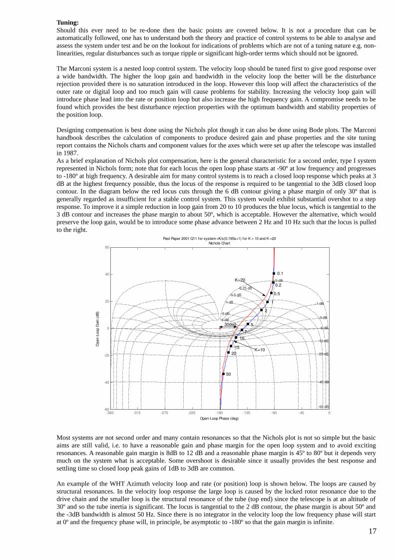
Designing compensation is best done using the Nichols plot though it can also be done using Bode plots. The Marconihandbook describes the calculation of components to produce desired gain and phase properties and the site tuningreport contains the Nichols charts and component values for the axes which were set up after the telescope was installedin 1987.As a brief explanation of Nichols plot compensation, here is the general characteristic for a second order, type I systemrepresented in Nichols form; note that for each locus the open loop phase starts at -90º at low frequency and progressesto -180º at high frequency. A desirable aim for many control systems is to reach a closed loop response which peaks at 3dB at the highest frequency possible, thus the locus of the response is required to be tangential to the 3dB closed loopcontour. In the diagram below the red locus cuts through the 6 dB contour giving a phase margin of only 30º that isgenerally regarded as insufficient for a stable control system. This system would exhibit substantial overshot to a stepresponse. To improve it a simple reduction in loop gain from 20 to 10 produces the blue locus, which is tangential to the3 dB contour and increases the phase margin to about 50º, which is acceptable. However the alternative, which wouldpreserve the loop gain, would be to introduce some phase advance between 2 Hz and 10 Hz such that the locus is pulledto the right.

Nichols Chart

Open­Loop Phase (deg)

Ope

n­Lo

op G

ain 

(dB

)

­360 ­315 ­270 ­225 ­180 ­135 ­90 ­45 0­60

­40

­20

0

20

40

60

 ­6 dB

 3 dB

 6 dB

 ­40 dB

 0.25 dB

 0.5 dB

 1 dB

 ­3 dB

 ­20 dB

 0 dB

 ­1 dB

 ­12 dB

 ­60 dB

Past Paper 2001 Q11 for system =K/s(0.195s+1) for K = 10 and K =20 

0.1 

0.2 

0.5 

1 

2 

5 

7 10 

15 20 

50 

30deg 

K=10 

K=20 

Most systems are not second order and many contain resonances so that the Nichols plot is not so simple but the basicaims are still valid, i.e. to have a reasonable gain and phase margin for the open loop system and to avoid excitingresonances. A reasonable gain margin is 8dB to 12 dB and a reasonable phase margin is 45º to 80º but it depends verymuch on the system what is acceptable. Some overshoot is desirable since it usually provides the best response andsettling time so closed loop peak gains of 1dB to 3dB are common.

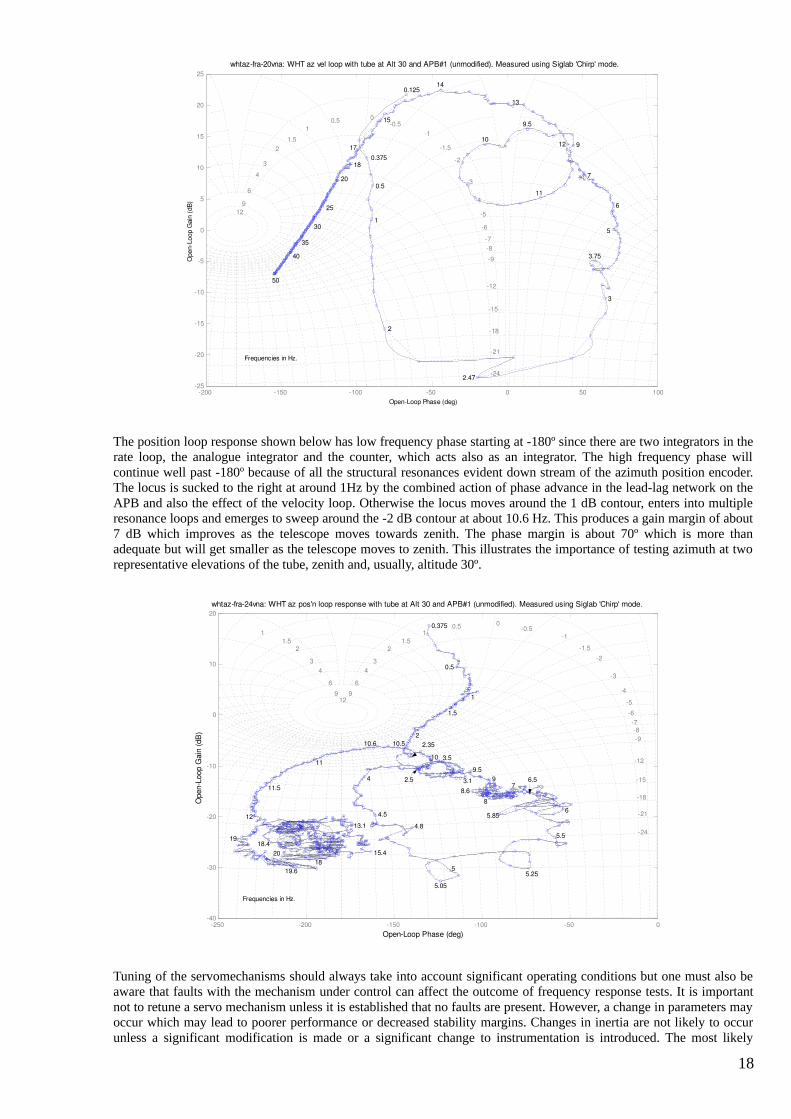
An example of the WHT Azimuth velocity loop and rate (or position) loop is shown below. The loops are caused bystructural resonances. In the velocity loop response the large loop is caused by the locked rotor resonance due to thedrive chain and the smaller loop is the structural resonance of the tube (top end) since the telescope is at an altitude of30º and so the tube inertia is significant. The locus is tangential to the 2 dB contour, the phase margin is about 50º andthe -3dB bandwidth is almost 50 Hz. Since there is no integrator in the velocity loop the low frequency phase will startat 0º and the frequency phase will, in principle, be asymptotic to -180º so that the gain margin is infinite.

17

Open­Loop Phase (deg)

Ope

n­Lo

op G

ain 

(dB

)

whtaz­fra­20vna: WHT az vel loop with tube at Alt 30 and APB#1 (unmodified). Measured using Siglab 'Chirp' mode.

­200 ­150 ­100 ­50 0 50 100­25

­20

­15

­10

­5

0

5

10

15

20

25

129

6

4

3

21.5

10.5 0

­0.5­1

­1.5

­2

­3

­4

­5

­6

­7­8

­9

­12

­15

­18

­21

­24

0.125 

0.375 

1 

0.5 

2 

2.47 

3 

3.75 

5 

6 

7 

9 

9.5 

10 

11 

12 

13 

14 

15 

17 

18 

20 

25 

30 

35 

40 

50 

Frequencies in Hz. 

The position loop response shown below has low frequency phase starting at -180º since there are two integrators in therate loop, the analogue integrator and the counter, which acts also as an integrator. The high frequency phase willcontinue well past -180º because of all the structural resonances evident down stream of the azimuth position encoder.The locus is sucked to the right at around 1Hz by the combined action of phase advance in the lead-lag network on theAPB and also the effect of the velocity loop. Otherwise the locus moves around the 1 dB contour, enters into multipleresonance loops and emerges to sweep around the -2 dB contour at about 10.6 Hz. This produces a gain margin of about7 dB which improves as the telescope moves towards zenith. The phase margin is about 70º which is more thanadequate but will get smaller as the telescope moves to zenith. This illustrates the importance of testing azimuth at tworepresentative elevations of the tube, zenith and, usually, altitude 30º.

Open­Loop Phase (deg)

Ope

n­Lo

op G

ain 

(dB

)

whtaz­fra­24vna: WHT az pos'n loop response with tube at Alt 30 and APB#1 (unmodified). Measured using Siglab 'Chirp' mode.

­250 ­200 ­150 ­100 ­50 0­40

­30

­20

­10

0

10

20

1299

66

4433

221.51.5

110.5 0

­0.5­1

­1.5

­2­2

­3­3

­4­4

­5­5

­6­6­7­7­8­8­9­9

­12­12

­15­15

­18­18

­21­21

­24­24

0.375 

0.5 

1 

1.5 

2 2.35 

2.5  3.1 

3.5 

4 

4.5 

4.8 

5 

5.05 

5.25 

5.5 

6 5.85 

6.5 7 

8 

8.6 

9 9.5 

10 

10.5 10.6 

11 

11.5 

12 

15.4 

13.1 

18 20 

19 

19.6 

18.4 

Frequencies in Hz. 

Tuning of the servomechanisms should always take into account significant operating conditions but one must also beaware that faults with the mechanism under control can affect the outcome of frequency response tests. It is importantnot to retune a servo mechanism unless it is established that no faults are present. However, a change in parameters mayoccur which may lead to poorer performance or decreased stability margins. Changes in inertia are not likely to occurunless a significant modification is made or a significant change to instrumentation is introduced. The most likely

18

change to be encountered is an increase or decrease in friction and the effect depends very much on the type andlocation of the friction. A change in static friction may introduce limit cycles in systems. A change in viscous frictioncan change the damping and hence make a system more or less stable. Another thing to beware off is the addition of asmall inertia through a large gear ratio or change in friction of a small device like an encoder which also couplesthrough a large gear ratio.

Initial problems may be identified through tracking tests, looking for evidence of encoder malfunction or of ‘new’frequencies being introduced which increase with velocity and therefore indicate gearing, motor or encoder problems.Frequencies which don’t shift with velocity may be structural resonances or may be due to closed loop peak responseexcitation produced by a shift in frequency response locus due to parameter changes. Simple tests can help todistinguish between these problems and are worth carrying out and analysing before committing to frequency responseanalysis.

19