Who Profits from Patents?

Rent-Sharing at Innovative Firms*

Patrick Kline

UC-Berkeley

Neviana Petkova

US Department of Treasury

Heidi Williams

MIT

Owen Zidar

Princeton

October 31, 2018

Abstract

This paper analyzes how patent-induced shocks to labor productivity propagate into worker compensationusing a new linkage of US patent applications to US business and worker tax records. We infer the causal effectsof patent allowances by comparing firms whose patent applications were initially allowed to those whose patentapplications were initially rejected. To identify patents that are ex-ante valuable, we extrapolate the excessstock return estimates of Kogan et al. (2017) to the full set of accepted and rejected patent applications basedon predetermined firm and patent application characteristics. An initial allowance of an ex-ante valuable patentgenerates substantial increases in firm productivity and worker compensation. By contrast, initial allowancesof lower ex-ante value patents yield no detectable effects on firm outcomes. Patent allowances lead firms toincrease employment, but entry wages and workforce composition are insensitive to patent decisions. On aver-age, workers capture roughly 30 cents of every dollar of patent-induced surplus in higher earnings. This shareis roughly twice as high among workers present since the year of application. These earnings effects are con-centrated among men and workers in the top half of the earnings distribution, and are paired with correspondingimprovements in worker retention among these groups. We interpret these earnings responses as reflecting thecapture of economic rents by senior workers, who are most costly for innovative firms to replace.

*We are very grateful to Joey Anderson, Ivan Badinski, Jeremy Brown, Alex Fahey, Sam Grondahl, Stephanie Kestelman, Tamri Mati-ashvili, Mahnum Shahzad, Karthik Srinivasan, and John Wieselthier for excellent research assistance, and to Daron Acemoglu, LawrenceKatz, Bentley MacLeod, John Van Reenen, four anonymous referees and seminar participants at Brown, Dartmouth, the LSE/IFS/STICERDseminar, Michigan, Michigan State, MIT, NBER Labor Studies, NBER Productivity, Northwestern, NYU, Princeton, Stanford, the ToulouseNetwork for Information Technology, UC-Berkeley, UC-Irvine, UIUC, Chicago Booth, and the Washington Center for Equitable Growthfor helpful comments. The construction of some of the data analyzed in this publication was supported by the National Institute on Agingand the NIH Common Fund, Office of the NIH Director, through Grant U01-AG046708 to the National Bureau of Economic Research(NBER); the content is solely the responsibility of the authors and does not necessarily represent the official views of the NIH or NBER.This work/research was also funded by the Ewing Marion Kauffman Foundation; the contents of this publication are solely the responsi-bility of the Grantee. Financial support from the Alfred P. Sloan Foundation, NSF Grant Numbers 1151497 and 1752431, the WashingtonCenter for Equitable Growth, the Kathryn and Grant Swick Faculty Research Fund, and the Booth School of Business at the University ofChicago are also gratefully acknowledged. Opinions expressed in the paper do not necessarily represent the views and policies of the USDepartment of the Treasury. Corresponding author: Williams; MIT Department of Economics; 50 Memorial Drive; E52-440; CambridgeMA 02142; heidiw@mit.edu.

1 Introduction

Competitive models of labor markets are predicated on the notion that firms have no power to set wages. How-

ever, there is mounting empirical evidence that firms contribute substantially to wage inequality among identically

skilled workers (Card, Heining, and Kline 2013; Card, Cardoso, and Kline 2016; Song et al. 2016; Sorkin 2018;

Jäger 2016; Goldschmidt and Schmieder 2017; Helpman et al. 2017; Abowd, McKinney, and Zhao 2018; Barth et

al. 2016). This emerging evidence has renewed interest in mechanisms through which variation in firm productivity

can influence worker pay (see Lentz and Mortensen 2010; Manning 2011 for reviews).

While a sizable empirical literature has documented that fluctuations in firm performance and worker com-

pensation are strongly related (Card et al., 2018), these correlations are open to widely varying interpretations.

Early studies (e.g., Christofides and Oswald 1992; Blanchflower, Oswald, and Sanfey 1996) estimated industry-

level relationships that could simply reflect competitive market dynamics. A second generation of studies (Van

Reenen 1996; Hildreth 1998; Abowd, Kramarz, and Margolis 1999) used firm-level data to study how shocks to

firm performance translate into worker pay, but was unable to adjust for potential changes in worker composition.

More recent work (Guiso, Pistaferri, and Schivardi 2005; Card, Devicienti, and Maida 2014; Card, Cardoso, and

Kline 2016; Carlsson, Messina, and Skans 2016; Lamadon 2016) adjusts for composition biases by examining

the comovement between changes in firm productivity and the wage growth of incumbent workers. However,

observational fluctuations in standard labor productivity measures are likely to reflect a number of factors (e.g.,

market-wide fluctuations in product demand, changes in non-pecuniary firm amenities, or drift in labor market

institutions) that can influence wages without necessarily signaling a violation of price-taking behavior by firms.

In this paper, we analyze how patent-induced shocks to firm performance propagate into worker compensation.

Patent allowances offer a useful source of variation because they provide firms with well-defined monopoly rights

that can yield a prolonged stream of potentially substantial economic rents. Standard models of frictional labor

markets (e.g., Pissarides 2000; Hall and Milgrom 2008; Pissarides 2009) suggest that these product market rents

will be shared with workers whenever the employment relationship is (re-)negotiated, yet surprisingly little is

known about how broadly patent-generated rents are shared in practice.

Our analysis relies on a new linkage of two datasets: (i) the census of published patent applications submitted

to the US Patent and Trademark Office (USPTO) between roughly 2001 and 2011 and (ii) the universe of US

Treasury business tax filings and worker earnings histories drawn from W2 and 1099 tax filings. The business

tax filings data offers a uniquely high-quality set of firm-level variables, from which we are able to construct

multiple measures of firm performance. Likewise, the business and worker tax filings provide a unique window

into compensation outcomes for many different types of workers, including firm officers and owners, who prevail

at the top of the income distribution (Smith et al., 2017).

1

We infer the causal effect of patent allowances by comparing firms whose applications were initially allowed

to those whose applications were initially rejected. Within so-called “art units” (technological areas designated by

the USPTO), firms with initially allowed and initially rejected applications submitted in the same year are found

to exhibit similar levels and trends in outcomes prior to their initial patent decision. We also document that initial

patent decisions are difficult to predict based on firm characteristics or geography, corroborating the view that these

decisions constitute truly idiosyncratic — as opposed to market level — shocks.

It is well-known that most patents generate little ex-post value to the firm (Pakes 1986; Hall, Jaffe, and Trajten-

berg 2001). We build on insights from two recent studies to identify a subsample of valuable patents that induce

meaningful shifts in firm outcomes at the time the patents are allowed. First, following the work of Farre-Mensa,

Hegde, and Ljungqvist (2017), we restrict our analysis to firms applying for a patent for the first time, for which

patent decisions are likely to be more consequential. Second, among this sample of first-time applicants, we build

on the analysis of Kogan et al. (2017) who use event studies to estimate the excess stock market return realized

on the grant date of US patents assigned to publicly traded firms. Specifically, we develop a methodology for

extrapolating Kogan et al.’s patent value estimates to the non-publicly traded firms in our sample, and to firms

whose patent applications are never granted. We use characteristics of firms and their patent applications that are

fixed at the time of application as the basis for extrapolating patent values, and show that these value estimates

are strong predictors of treatment effect heterogeneity in our sample. These value estimates also provide us with

an additional validation of our research design: patents with low predicted value are found to have economically

small and statistically insignificant effects on firm performance and worker compensation.

Using these data, we then investigate the consequences of obtaining an ex-ante valuable patent allowance for

firm performance and worker compensation, and relate our findings to different explanations for the propagation

of firm-specific shocks into worker wages. Corroborating recent research based on US Census data (Balasubrama-

nian and Sivadasan 2011), we find that firm size and average labor productivity rise rapidly in response to initial

allowances of ex-ante valuable patents. The average wage and salary income of workers at these firms rises in

tandem with measures of average labor productivity. An allowance of a patent application in the top quintile of

ex-ante predicted value raises firm-level surplus — defined as the sum of W2 earnings and business earnings before

interest, taxes, and depreciation — by roughly $12,400 per W2 employee per year, while W2 earnings at the firm

rise by approximately $3,700 per worker per year.

Patent allowances not only raise average earnings at assignee firms, but also exacerbate within-firm inequality

on a variety of margins. Earnings impacts are heavily concentrated among employees in the top quartile of the

within-firm earnings distribution and among employees listed on firm tax returns as “firm officers.” Likewise, we

find that the earnings of owner-operators rise more than those of other employees. Earnings of male employees rise

strongly in response to a patent allowance, while the earnings of female employees are less responsive to patent

2

decisions.

A handful of previous studies have investigated how inventor wages change in response to patent applications

or patent grants (Toivanen and Väänänen 2012; Depalo and Di Addario 2014; Bell et al. 2016; Aghion et al.

2017). Consistent with these results, we find that the earnings of “inventors” — defined as employees ever listed

as inventors on a patent application as in Bell et al. (2016) — respond to patent allowance decisions. Inventor

earnings are more responsive to patent allowance decisions than are the earnings of non-inventors, similar to

the findings presented in contemporaneous work by Aghion et al. (2018) which analyzes how inventor and non-

inventor earnings in Finnish firms evolve before and after patent applications are filed.

While these impacts on firm aggregates could, in principle, be confounded by compositional changes, we find

no evidence that innovative firms upgrade the quality of their workforce in response to patent allowances. Although

patent allowances lead firms to expand by hiring slightly younger workers, the average prior earnings of both new

hires and firm separators is unaffected by patent decisions, suggesting that there are no major changes in the skill

composition of worker inflows to or outflows from the firm on a year-to-year basis.

Different theoretical frameworks offer divergent predictions about how firm-specific shocks will affect the

wages of new and incumbent workers. Empirically, the earnings of workers who were employed by the firm in the

year of application respond very strongly to patent decisions. Having a valuable patent allowed raises the average

earnings of these “firm stayers” by roughly $7,800 — or approximately 11% — per year. These gains appear to be

concentrated among firm stayers who, in the year of application, were located in the top half of the firm’s earnings

distribution. We also find that the earnings of male firm stayers respond more strongly to patent allowances than

those of female firm stayers, which are estimated to be positive, albeit somewhat imprecise. By contrast, we are

unable to detect any response of entry wages to patent allowances, which is inconsistent with the predictions of

both static wage posting models and traditional bargaining models involving Nash-style surplus splitting at the time

of hiring (Pissarides 2000; Hall and Milgrom 2008; Pissarides 2009). While some dynamic wage posting models

(e.g., Postel-Vinay and Robin 2002) can generate drops in entry wages in response to a productivity increase, these

models predict greater wage growth for new hires, a phenomenon for which we also find no evidence. A candidate

explanation for such “insider/outsider” distinctions in earnings impacts is that the wage fluctuations of incumbent

workers represent changes in market perceptions of a worker’s underlying ability (Gibbons and Murphy 1992;

Holmström 1999). However, we find much smaller and statistically insignificant earnings effects on workers who

leave the firm, suggesting that our results are unlikely to be driven by public learning about worker quality.

To interpret our findings, we sketch a simple model in which incumbent workers are imperfectly substitutable

with new hires. As in Becker (1964), Stevens (1994), and Manning (2006), this mechanism provides an avenue for

incumbents to extract rents from the firm in the form of wage premia. Motivated by this framework, we fit a series of

“rent-sharing” specifications analogous to standard cost-price pass-through specifications used to study imperfect

3

competition in product markets (Goldberg and Hellerstein, 2013; Weyl and Fabinger, 2013; Gorodnichenko and

Talavera, 2017). Using patent decisions as an instrument for firm surplus, we find that worker earnings rise by

roughly 29 cents of every dollar of patent allowance-induced surplus, with an approximate elasticity of 0.35,

which is comparable to the earlier estimates of Abowd and Lemieux (1993) and Van Reenen (1996) that were

based on firm-level aggregates. Importantly, failing to instrument for surplus yields smaller elasticities, closer

to those in the recent studies reviewed by Card et al. (2018) that assume statistical innovations to average labor

productivity constitute structural productivity shocks. Consistent with our model, rent-sharing with firm stayers is

more pronounced than it is with average workers: stayers capture roughly 61 cents of every dollar of surplus for an

approximate elasticity of 0.56. When we exclude employees ever listed as inventors on a patent, pass-through to

firm stayers falls to roughly 48 cents with a corresponding elasticity of 0.5. Though this elasticity estimate is larger

than what has been found by most previous studies, its 90% confidence interval encompasses many estimates in

the literature.

In our model, firms share rents with incumbent workers to increase the odds of retaining them. We provide

event study evidence that retention rises in response to patent allowances, with larger responses among workers in

the top half of the earnings distribution. The fact that groups experiencing the largest earnings responses exhibit

the largest retention responses strongly suggests that the earnings fluctuations we measure constitute rents, rather

than, say, risk-sharing arrangements that hold workers to a participation constraint (Holmström 1979, 1989). Using

the patent decision as an instrument for wages, we estimate a retention-wage elasticity of roughly 1.2, with a 90%

confidence interval ranging from 0.46 to 3.1. When converted to a separation-wage elasticity, our point estimate

lies near the middle of the range of quasi-experimental estimates reviewed in Manning (2011).

Viewed through the lens of our model, our point estimates imply that incumbent workers capture roughly 73%

of their replacement costs in wage premia. We also estimate that the marginal replacement cost of an incumbent

worker at a firm receiving a patent allowance is roughly equal to a new hire’s annual earnings. These findings

suggest that separations of key personnel can be extremely costly to innovative firms, even when these employees

are not themselves inventors. More broadly, our results suggest that the influence of firm conditions on worker

wages depends critically on their degree of replaceability, which may be influenced both by the duration of the

relationship between the worker and firm and by a worker’s position within the firm hierarchy, issues which have

been emphasized in recent empirical studies of wage setting at European firms by Buhai et al. (2014), Jäger (2016),

and Garin and Silverio (2017). In contrast with European settings, however, the legal barriers to hiring and firing

workers are comparatively minimal for the set of newly innovative US firms which are the focus of our analysis.

The fact that seniority appears to mediate the propagation of firm shocks into worker earnings even in this sample

of firms strongly suggests an important role for relationship-specific investments in the generation of labor market

rents.

4

2 Interpreting Wage Fluctuations

In this section, we sketch a simple model of wage determination designed to interpret the propagation of firm-

specific productivity shocks into wages. Our model is tailored to the newly-innovative firms that are the focus of

our empirical analysis. For the purposes of motivating our model, two features of these firms are notable. First,

these firms are relatively small: the median firm in our estimation sample employs 17 workers in the year of

its first patent application.1 Such firms seem unlikely to possess significant market power over new hires or to

have reputations that allow them to credibly commit to backloaded compensation schemes. Second, the innovative

work conducted at these firms is necessarily specialized and proprietary in nature, likely making it costly to replace

incumbent employees with new hires. As in Becker (1964), Stevens (1994), and Manning (2006), the imperfect

substitutability of incumbent workers with new hires provides an avenue for incumbents workers to extract rents

from the firm in the form of wage premia.

Our model yields a linear wage-setting rule similar to those found in many search models with multi-lateral

bargaining (Pissarides 2000; Cahuc and Wasmer 2001; Acemoglu and Hawkins 2014), as well as in much of

the classic literature on union wage bargaining (Brown and Ashenfelter 1986). We use this framework to motivate

standard empirical “rent-sharing” specifications and to clarify the endogeneity problems that arise when estimating

the transmission of firm-specific shocks to wages. We then discuss the assumptions under which patent allowance

decisions can facilitate the identification of economic parameters of interest.

2.1 Preliminaries

We work with a one period model. Each firm j ∈ {1, ...,J} begins the period with I j incumbent workers and

a non-wage amenity value A j capturing factors such as geographic location and work environment. The firm can

hire as many new workers as desired at competitive market wage wmj = wm (A j). As in classic hedonic models

(e.g., Rosen, 1986), the wage demanded by new hires will tend to be decreasing in the value of these amenities(i.e., ∂

∂A jwm (A j)≤ 0

), which leads entry wages to vary by firm despite the perfectly competitive nature of this

market.

Hiring N j new workers requires paying a training and recruiting cost c(N j, I j). The function c(., .) exhibits

constant returns to scale, which implies

c(N j, I j) = c(N j/I j) I j.

We assume c(.) is twice differentiable and convex.

1While the firms in our sample are small relative to, e.g., firms included in the Compustat data, they should not be thought of asanomalously small in size. Axtell (2001) finds using Economic Census data that the modal US firm size is 1 employee, and the median is 3(4 if size 0 firms are not counted).

5

The firm chooses a wage wIj ≥ wm

j for incumbent workers at the beginning of the period. After the wage is

posted, incumbent workers receive outside job offers. These offers are non-verifiable, in part because they may

involve non-wage amenities, and therefore cannot be matched. However, the firm knows the offers have wage-

equivalent values drawn from the following translated Beta distribution

G j (ω) =

(ω−wm

j

w̄ j−wmj

)η

for ω ∈[wm

j , w̄ j],

where w̄ j > wmj is the maximum value of an outside offer. As η grows, offers become concentrated around w̄ j,

while, as η tends towards zero, offers become concentrated around wmj .

Workers receiving outside offers with value greater than the incumbent wage separate from the firm. Conse-

quently, G j

(wI

j

)I j incumbent workers are retained for production activities. Note that η can therefore be inter-

preted as the elasticity of worker retention with respect to the incumbent wage premium wIj−wm

j .

At the end of the period, the firm produces Q j = TjL j units of output where L j = N j +G j

(wI

j

)I j gives the

number of retained workers and Tj gives the firm’s “physical” productivity. Output is sold on a monopolistically

competitive product market with inverse product demand Pj (Q j) = P0j Q−1/ε

j where P0j > 0 is a firm-specific con-

stant capturing the firm’s product market power and ε > 1 gives the elasticity of demand. After selling its output

and paying the retained workers, the firm shuts down.

2.2 The firm’s problem

The firm chooses the number of new hires N j and an incumbent wage wIj to maximize profits. Formally, its

problem is to:

max{wI

j,N j}P0

j[Tj(G j(wI

j)

I j +N j)]1−1/ε︸ ︷︷ ︸

revenue

−c(N j/I j) I j︸ ︷︷ ︸training cost

−wmj N j−wI

jG(wI

j)

I j︸ ︷︷ ︸wage bill

.

At an optimum, the firm equates the marginal cost of a new hire to her marginal revenue product (MRPj):

wmj + c′ (N j/I j) = (1−1/ε)

P(Q j)Q j

L j≡MRPj. (1)

Note that the marginal cost of a hire exceeds the market wage by the amount of the training/recruiting cost

c′ (N j/I j), which is increasing in the gross hiring rate N j/I j.

For incumbent wages, the first order condition can be written:

MRPj = wIj +

(wI

j−wmj)/η︸ ︷︷ ︸

inframarginal wage cost

. (2)

6

As in monopsony models, the firm equates the marginal revenue product of an incumbent worker to her marginal

factor cost, which consists of her wage wIj plus a term capturing the costs of raising wages for inframarginal

incumbents. As the retention elasticity η approaches infinity, this term collapses to the standard neoclassical

requirement that the marginal revenue product of an incumbent worker equal her wage.

2.3 Rent Sharing

Subtracting equations (1) and (2), we arrive the following expression for the incumbent wage premium:

wIj−wm

j =η

1+ηc′ (N j/I j) . (3)

Incumbents are paid a premium over new hires in proportion to their marginal training/recruiting costs c′ (N j/I j).

When c′ (N j/I j) = 0 incumbent workers are replaceable. In this case, the firm views new hires and incumbents as

perfect substitutes and pays them equivalently. The fraction η

1+η∈ [0,1] plays the role of the exploitation index in

classic monopsony models (Manning, 2011) where η would correspond to a firm-specific labor supply elasticity.

As the retention elasticity η approaches infinity, incumbents capture their full (marginal) replacement cost in the

form of elevated wages. As η tends towards zero, the outside options of incumbents deteriorate, allowing the firm

to retain them at the market wage wmj and capture the rents in the employment relationship.

Plugging (3) into (1) yields an expression for the incumbent wage that is useful for motivating our empirical

rent-sharing specifications:

wIj =

11+η

wmj +

η

1+ηMRPj (4)

= (1−θ)wmj +θMRPj

where θ = η

1+η. Workers are paid a θ -weighted average of their marginal productivity and the market wage wm

j .

Rewriting θ =wI

j−wmj

MRPj−wmj

illustrates the link to models with Nash wage bargaining in which θ gives the fraction

of marginal match surplus paid out in wage premia.2 As the retention elasticity η increases, θ rises and workers

capture more of the surplus.

The parameter θ has a clear causal interpretation: a dollar increase in marginal productivity yields a θ -cent pay

increase for incumbents. It is useful to review briefly why marginal products can vary in this model. In the special

case where incumbents are replaceable (c′ (N j/I j) = 0), (1) implies the marginal revenue product would be pinned

2Stole and Zwiebel (1996) propose a multilateral bargaining framework where workers and firms also bargain over infra-marginalproducts. This bargaining concept is embedded in a search and matching framework by Acemoglu and Hawkins (2014). Given ourassumption of a constant product demand elasticity, the wage rule that results from the Stole-Zwiebel approach is analogous to equation (4)with the modification that the weights on the reservation wage and marginal revenue product need not sum to 1.

7

to the market wage wmj . Hence, there would be no scope for fluctuations in MRPj other than due to shifts in the

amenity vector A j. But when incumbents are not replaceable, MRPj will also respond to fluctuations in “revenue

productivity” P0j Tj. As described below, our empirical approach uses variation in patent allowances to isolate the

variation in MRPj that arises due to exogenous fluctuations in revenue productivity.

2.4 Estimating pass-through

We can operationalize equation (4) by plugging in the definition of MRPj to get:

wIj = (1−θ)wm

j +θ

(1− 1

ε

)PjQ j

L j

= (1−θ)wmj +πS j. (5)

The last line of this expression is a standard empirical rent-sharing specification relating incumbent wages at the

firm to a measure of average labor productivity S j =PjQ j

L j, which we refer to as gross surplus per worker.

The parameter π = θ(1− 1

ε

)governs pass-through of gross surplus to wages and can be thought of as the labor

market analog of cost-price pass-through coefficients often used to study imperfect competition in product markets

(Goldberg and Hellerstein 2013; Weyl and Fabinger 2013; Gorodnichenko and Talavera 2017). The term(1− 1

ε

)is an adjustment factor that converts average labor productivity to marginal labor productivity. While π is our

primary parameter of interest, we also explore calibrations of ε and consider the implied values of the structural

rent-sharing coefficient θ .

Card et al. (2018) review several studies that use panel methods to assess the relation between the wage growth

of incumbent workers and fluctuations in various measures of firm surplus. Equation (5) suggests such specifi-

cations will suffer from omitted variables bias whenever surplus fluctuations are correlated with changes in the

market wage wmj . For example, shocks to firm productivity may contain a market-wide component. If all firms

in a market become more productive, market wages will rise. This possibility would lead to a misattribution of

market-level wage adjustments to rent-sharing and a corresponding upward bias in OLS estimates of π .

A different class of potential biases arises from unobserved shocks to the amenity value of a firm. Suppose the

work environment at a firm improves and leads to a decrease in wmj . This improvement will lead, ceteris paribus,

to an increase in firm scale, which will tend to depress average labor productivity through drops in the product

price Pj (Q j). Consequently, such shocks will induce a positive covariance between wmj and S j = P0T 1−1/ε

j L−1/ε

j

and hence lead to an overstatement of the degree of rent-sharing. However, unobserved amenity shocks could also

exert a direct effect on productivity. For example, a recent empirical literature finds that variation in management

practices affects both worker morale and productivity (Bloom and Van Reenen 2007; Bender et al. 2018). A

new manager who motivates workers could plausibly raise total factor productivity Tj while lowering the market

8

wage wmj via increases in the amenity value A j of the firm. This possibility would lead to an under-estimate of

rent-sharing as the productivity shock is accompanied by an unobserved amenity shock.

2.5 Instrumenting with Patent Decisions

To circumvent these endogeneity problems, we use the initial decision of the US Patent and Trademark Office

(USPTO) on a firm’s first patent application as an instrument for the firm’s surplus.3 Patents could influence

average labor productivity through two channels, both of which provide valid identifying variation. First, a patent

grant could raise a firm’s product price intercept P0j by creating a barrier to competition by rival firms.4 Second, a

patent grant could raise a firm’s TFP Tj by making it profitable for the firm to implement the patented technology.

We document below that within observable strata, the USPTO’s initial decision on a given patent application

is unrelated to trends in firm performance, implying that initial patent decisions are as good as randomly assigned

with respect to counterfactual changes in firm outcomes. Consistent with this evidence, we also document below

that it is hard to predict initial decisions using firm characteristics in the year of application. Finally, we assume

that patent decisions are uncorrelated with fluctuations in the market wage wmj . In the model above, this condition

is sufficient to ensure that instrumenting S j with the patent allowance isolates exogenous variation in revenue

productivity P0j Tj and identifies the pass-through parameter π .

The assumption that patent decisions are uncorrelated with fluctuations in wmj merits further discussion in our

setting as several violations of this condition are conceivable, most of which are not explicitly modeled in the above

framework. A first concern is that patent allowances might lead the firm to demand more hours from workers, in

which case wmj would rise. However, we would expect this to be a short-run phenomenon that dissipates as the

firm expands towards its new target size, and we find no evidence of such wage dynamics in the data. A different

sort of violation would occur if patents shift expectations about firm growth and therefore about the future earnings

growth of workers. This sort of mechanism arises in dynamic wage posting models with offer matching (Postel-

Vinay and Robin 2002) and would imply that wmj falls in response to an allowance. However, such a violation

would also imply that initial allowances should raise the wage growth of new hires, an assertion for which we find

no empirical support.

A second concern is that initial allowance decisions might be geographically correlated, in which case in-

strumenting with initial allowances might pick up market-wide fluctuations in wmj . We show below however that

3Van Reenen (1996) also investigated patents as a source of variation, but found them to be a relatively weak predictor of firm profitsin his sample of firms (see his footnote 11). This finding is in keeping with the notion that most patents generate little ex-post value to thefirm (Pakes 1986), motivating our focus on ex-ante valuable patent applications as described in Section 5. A natural alternative empiricalstrategy in our setting would be to use the leniency of the patent examiner assigned to review the patent application as an instrument, as inSampat and Williams (forthcoming). Unfortunately, this strategy reduces the precision of our estimates to the point of being uninformative.

4Perhaps the classic example is patents on branded small molecule pharmaceuticals. In the absence of patents, many branded pharma-ceuticals would experience near-immediate entry of generic versions which compete with branded pharmaceuticals at close to marginalcost prices.

9

the intra-class correlation of initial patent allowances within geography and sector is indistinguishable from zero,

which suggests that allowances are best thought of as truly firm-specific shocks. We also find no impact of patent

allowances on the earnings of workers in their first year of employment with a firm, which should provide a

reasonable proxy of the market wage wmj . Since all of the above concerns involve correlations between patent

allowances and fluctuations in the market wage wmj , this provides a strong corroboration of the exogeneity of the

patent allowance instrument.

A final concern is that firms may respond to patent decisions by changing the composition of their workforce.

By leveraging the panel structure of our data, we can directly investigate whether firms change their composition

of new hires (or separations) in response to patent allowances. We also address this concern by analyzing the wage

growth of incumbent workers, which by construction differences out any selection on time invariant characteristics.

In practice, we find that such adjustments have little effect on our estimates of the pass-through parameter π .

3 Data and Descriptive Statistics

To conduct our empirical analysis, we construct a novel linkage of several administrative databases, which

provides us with panel data on the patent filings, patent allowance decisions, and outcomes of US firms and

workers.

3.1 USPTO Patent Applications

We begin with public-use administrative data on the universe of patent applications submitted to the US Patent

and Trademark Office (USPTO) since late 2000.5 We link these published US patent applications with several

USPTO administrative datasets. Because published patent applications are not required to list the assignee (owner)

of the patent, approximately 50% of published patent applications were originally missing assignee names. We

worked with the USPTO to gain access to a separate public-use administrative data file that allows us to fill in

assignee names for most of these applications. The public-use USPTO PAIR (Patent Application Information

Retrieval) administrative data records the full correspondence between the applicant and the USPTO, allowing us

to infer the timing and content of the USPTO’s initial decision on each patent application as well as other measures

of USPTO and applicant behavior. Details on these and the other patent-related data files that we use are included

in Appendix A.

Panel A of Table 1 describes the construction of our patent application sample. Our full sample consists of

5The start date of our sample is determined by the American Inventors Protection Act of 1999, which required publication of nearly thefull set of US patent applications filed on or after 29 November 2000. We say “nearly” because our sample misses patent applications thatopt out of publication; Graham and Hegde (2014) use internal USPTO records to estimate that around eight percent of USPTO applicationsopt out of publication.

10

the roughly 3.6 million USPTO patent applications filed on or after 29 November 2000 that were published by

31 December 2013; we restrict attention to applications filed on or before 31 December 2010 in order to limit the

impact of censoring. We drop around 400,000 applications that are missing assignee names and therefore cannot

be matched to business tax records. We also limit our sample to standard (so-called “utility”) patents.6

To focus on a subset of firms for which patent allowances are most likely to induce a meaningful shift in firm

outcomes, we make several restrictions that aim to limit our sample to first-time patent applicants. First, we drop

so-called “child” applications that are derived from previous patent applications. Second, we retain the earliest

published patent application observed for each assignee in our sample.7 Finally, we exclude assignees which we

observe to have had patent grants prior to the start of our published patent application sample.8 Ideally, we would

exclude assignees that had patent applications (not just patent grants) prior to the start of our published patent

application sample, but unsuccessful patent applications filed before 29 November 2000 are not publicly available.

These restrictions leave a sample of around 96,000 patent applications, which we then attempt to match to our US

Treasury business tax files.

3.2 Treasury Tax Files

We link US Treasury business tax filings with worker-level filings. Annual business tax returns record firm

outcomes from Form 1120 (C-Corporations), 1120S (S-Corporations), and 1065 (Partnership) forms, and cover

the years 1997-2014. The key variables that we draw from the business tax return filings are revenue, value added,

EBITD (earnings before interest, taxes, and deductions), and labor compensation; each of these is defined in more

detail in Appendix A.

We link these business tax returns to worker-level W2 and 1099 filings in order to measure employment and

compensation for employees (e.g., wage bill) and independent contractors, respectively, at the firm-year level. The

relevant variables are defined in more detail in Appendix A. We winsorize all monetary values in the tax files from

above and below at the five percent level, which is standard when working with the population of US Treasury

business tax files (see, for example, DeBacker et al. 2016; Yagan 2015). Since our analysis focuses on per-worker

outcomes, we winsorize outcomes on a per-worker basis.

To distinguish employment and compensation for inventors and non-inventors, we use Bell et al.’s (2016)

merge of inventors listed in patent applications to W2 filings. Inventors are defined as individuals ever appearing

6Utility patents, also known as “patents for invention,” comprise approximately 90% of USPTO-issued patent documents in recent years;see https://www.uspto.gov/web/offices/ac/ido/oeip/taf/patdesc.htm for details.

7Because USPTO procedure assigns application numbers sequentially, we break ties in the cases in which a given assignee submitsmultiple applications on the same day by taking the smallest application number.

8We search for such patent grants going back to 1976, the date with electronic patent grant records are most easily available. Given thefirms in our sample, the likelihood that a firm had a patent granted prior to 1976 seemed sufficiently small not to warrant a more extensiveattempt to match to earlier patent grants.

11

in the Bell et al. (2016) patent application-W2 linkage, rather than individuals listed as inventors on the specific

patent application relevant to a given firm in our sample.

3.3 Linkage Procedure

We build on the name standardization routine used by the National Bureau of Economic Research (NBER)’s

Patent Data Project (https://sites.google.com/site/patentdataproject/) to implement a novel firm

name-based merge of patent assignees to firm names in the US Treasury business tax files. Specifically, we

standardize the firm names in both the patent data and (separately) the US Treasury business tax files in order

to infer that, e.g., “ALCATEL-LUCENT U.S.A., INC.,” “ALCATEL-LUCENT USA, INCORPORATED,” and

“ALCATEL-LUCENT USA INC” are all in fact the same firm. We then conduct a fuzzy merge of standardized

assignee names to standardized firm names in the business tax files using the SoftTFIDF algorithm based on a

Jaro-Winkler distance measure. This merge is described in more detail in Appendix A.

To assess the quality of our merge, we conducted two quality checks: first, we validate against a hand-coded

sample; and second, we validate against the inventor-based linkage of Bell et al. (2016). As described in Appendix

A, the results of these validation exercises suggest that our merge is of relatively high quality, with type I and II

error rates on the order of five percent.

Panel B of Table 1 describes our linkage between the USPTO patent applications data and the US Treasury

business tax files. Of the around 96,000 patent applications we attempt to match to the US Treasury business tax

files, we match around 40,000 patent applications. The USPTO estimates that in 2015 approximately 49.6% of

USPTO patent grants were filed by US-based assignees, which implies our match rate to US-tax-paying entities is

on the order of 83%.9 These 40,000 patent applications are matched to around 40,000 standardized firm names in

the US Treasury business tax files, which corresponds to 82,000 firms (employer identification numbers, or EINs).

We build the analysis sample from these 82,000 EINs in four steps. Our goal here is to construct a unique and

well-defined match between patent applications and firms in a subset of firms for which patent allowances are most

likely to induce a meaningful shift in firm outcomes. First, we attempt to restrict our post-merge tax analysis sample

to first-time patent applicants by retaining the earliest-published patent application observed for each EIN, and by

excluding EINs which we observe to have had patent grants prior to the start of our published patent application

sample. Second, in cases in which there are multiple EINs for a standardized name in the tax files, we keep the EIN

with largest revenue in the year that the patent application was filed. Third, we restrict attention to “active” firms,

defined as EINs that have a positive number of employees in the year of application and non-zero, non-missing

total income or total deductions in the year the patent application was filed and in the three previous years. This

9These USPTO estimates, which are based on the reported location of patent assignees, are available here: https://www.uspto.gov/web/offices/ac/ido/oeip/taf/own_cst_utl.htm.

12

restriction allows us to investigate pre-trends in our outcome variables among economically relevant firms. Fourth,

we limit attention to EINs with less than 100 million in revenue in 2014 USD in the year of patent application.

This step, which eliminates firms in the top centile of the firm size distribution, allows us to avoid complexities

related to the largest multinational companies and focus on firms for whom patent allowance decisions are more

likely to be consequential.10 These restrictions leave us with a sample of 9,732 patent applications, each uniquely

matched to one EIN in the US Treasury business tax files. It is worth noting that focusing on such a small subset of

firms is common in analyses such as ours. For example, Kogan et al. (2017) start with data on 7.8 million granted

patents, which they winnow down to a final sample of 5,801 firms with at least one patent.

3.4 Measuring Surplus

As described in Card et al. (2018), empirical rent-sharing estimates are often sensitive to a number of measure-

ment issues, the most prominent of which is the choice of rent measure. In keeping with equation (5), we rely on a

gross surplus measure of rent that differs from “match surplus” due to the absence of data on workers’ reservation

wages. Letting Π j denote the firm’s economic profits, the model of Section 2 implies the firm’s total gross surplus

can be written:

S jL j = wmj N j +wI

jG(wI

j)

I j︸ ︷︷ ︸wage bill

+ Π j︸︷︷︸profits

+ c(N j/I j) I j︸ ︷︷ ︸training/recruiting costs

.

To measure this theoretical concept in the tax data, we use the sum of the firm’s W2 earnings in a year and

its earnings before interest, tax, and depreciation (EBITD). Though firms sometimes report negative EBITD, this

surplus measure is usually positive and provides a plausible upper bound on the flow of resources capable of being

captured by workers. Note that this measure is theoretically justified by the presumption that firms do not claim

deductions on training costs; i.e., that EBITD captures the sum Π j + c(N j/I j) I j.11

For comparison with past work, we also report results that use a value added measure of surplus. Our approx-

imation to value added comes from line 3 of Form 1120, which deducts from gross sales, returns and allowances,

and the cost of goods sold. This measure suffers from the disadvantage that it may include a number of additional

unobserved firm costs including rents, advertising, and financing fees that that are likely unavailable for capture by

workers.10Statistics for firm size distribution are from Smith et al. (2017). Specifically, in the full population of C-corporations, S-corporations,

and Partnerships with positive sales and positive W2 wage bills, $100 million in revenue in 2014 USD falls in the top one percent of firms.11Unlike some other capital expenses and costs related to intangibles, which can be amortized, firms typically can not amortize and deduct

costs related to training. Specifically, section 197 on intangibles includes workforce in place (e.g., “experience, education, or training”’)and business books and records (e.g., “intangible value of technical manuals, training manuals or programs”) in the list of assets that cannotbe amortized for most firms. See https://www.irs.gov/pub/irs-pdf/p535.pdf for additional details.

13

3.5 Summary Statistics

Table 2 tabulates summary statistics on our firm and worker outcomes in each of two samples: our analysis

sample of matched patent applications/firms (N=9,732), and our sub-sample of matched patent applications/firms

for which the patent applications are in the top quintile of predicted value (N=1,946), which will be defined in the

next section. All summary statistics are as of the year the patent application was filed.

Panel A documents summary statistics on firm-level outcomes. In our analysis sample, the median firm gen-

erated around three million dollars in revenue, employed 17 workers, and reported roughly $7,000 in EBITD per

worker. Approximately 8% of patent applications are initially allowed. Panel B documents summary statistics

on worker-level outcomes. The median firm in our analysis sample paid $48,000 in annual earnings per W2 em-

ployee, employed a workforce that is approximately 75% male, and issued 2.5% of its W2s to individuals listed

as inventors on at least one patent application. Contract work turns out to be relatively uncommon in this sample,

with 1099s constituting only about 10% of the sum of W2 and 1099 employment for the median firm.

4 Institutional Context: Initial Patent Decisions

The US Patent and Trademark Office (USPTO) is responsible for determining which — if any — inventions

claimed in patent applications should be granted a patent. Patentable inventions must be patent-eligible (35 U.S.C.

§101), novel (35 U.S.C. §102), non-obvious (35 U.S.C. §103), useful (35 U.S.C. §101), and the text of the appli-

cation must satisfy the disclosure requirement (35 U.S.C. §112). When patent applications are submitted to the

USPTO, they are routed to a central office which directs the application to an appropriate “art unit” that special-

izes in the technological area of that application. For example, art unit 1671 reviews applications related to the

chemistry of carbon compounds, whereas art unit 3744 reviews applications related to refrigeration. The manager

of the relevant art unit then assigns the application to a patent examiner for review. If the examiner issues an initial

allowance, the inventor can be granted a patent. If the examiner issues an initial rejection, the applicant has the op-

portunity to “revise and resubmit” the application, and the applicant and examiner may engage in many subsequent

rounds of revision (see Williams 2017 for more details).

Our empirical strategy focuses on contrasting firms that receive an initial allowance to other firms that applied

for a patent but received an initial rejection. Empirically, most patent applications receive an initial decision within

three years of being filed (see Appendix Figure C.1). While some applications that are initially rejected receive

a patent grant relatively quickly, the modal application that is initially rejected is never granted a patent (see

Appendix Figure C.2).

Because our empirical strategy will contrast firms whose applications are initially allowed to those whose

applications are initially rejected, having some sense of what predicts initial allowance decisions is useful. Table

14

3 reports least squares estimates of the probability of an initial allowance as a function of firm characteristics in

the year of application. Column (1a) shows that predicting initial allowances is surprisingly difficult. Applications

from firms with more W2 employees are somewhat less likely to be initially allowed, as are those from firms with

higher value added per worker. Jointly, the covariates are statistically significant. Column (1b) adds art unit by

application year fixed effects that control for technology-specific changes over time. This simple addition renders

all baseline covariates statistically insignificant both individually and jointly, which provides some assurance that

initial patent decisions are not strongly dependent on baseline firm performance. Given this empirical evidence,

we proceed by assuming that any remaining selection is on time-invariant firm characteristics that can be captured

by firm fixed effects.

A separate concern has to do with whether initial allowances are best thought of as idiosyncratic or market-level

shocks. Seminal work by Jaffe, Trajtenberg, and Henderson (1993) demonstrated that patent citations are highly

localized geographically. To test whether initial allowances are also geographically clustered, we fit linear random

effects models to the initial allowance decision. Appendix Table C.1 reports intraclass correlations at various levels

of geography before and after subtracting off art unit by application year mean allowance rates. In either case, the

within-state correlation is estimated to be zero, while the correlation within five-digit ZIP codes is quite low (0.07-

0.10) and statistically indistinguishable from zero. These findings indicate that initial allowances are best thought

of as truly idiosyncratic firm-specific shocks that are unlikely to elicit market-wide wage responses.

5 Detecting Valuable Patents

The value distribution of granted patents is heavily skewed (Pakes 1986), which suggests that low-value patent

applications — if granted — are unlikely to generate meaningful shifts in firm outcomes. Constructing a measure

of the ex-ante value of patent applications enables us to focus our analysis on patent applications that are likely to

induce changes in firm behavior.

A variety of metrics have been proposed as measures of the value of granted patents, including forward patent

citations (Trajtenberg 1990), patent renewal behavior (Pakes 1986; Schankerman and Pakes 1986; Bessen 2008),

patent ownership reassignments (Serrano 2010), patent litigation (Harhoff, Scherer, and Vopel 2003), and excess

stock market returns (Kogan et al. 2017). These value measures encounter three challenges in our empirical context.

First, these measures are only defined for granted patents, whereas we would like to take advantage of data on patent

applications, including those that are ultimately unsuccessful. Second, most of these measures arguably correspond

to a measure of social value — or social spillovers, in the sense of social value minus private value — whereas

we are more interested in measuring firms’ private value of a patent. This issue arises most sharply with forward

patent citations, which are typically used as a measure of spillovers (e.g., Bloom, Schankerman, and Van Reenen

15

2013). Third, all of these measures are defined ex-post: citations, renewals, reassignments, and litigation are often

measured many years after the initial patent award. But in our context — as in Kogan et al. (2017) — what is

arguably more relevant is the expected private value of the patent at the time of the patent application or patent

grant.

To this end, we build on the recent analysis of Kogan et al. (2017) (henceforth, KPSS), who measure the

high-frequency response of stock prices around the date of patent grant announcements to estimate the value of

patent grants that are awarded to publicly traded companies. We estimate a simple statistical model designed to

extrapolate their estimates to non-publicly traded companies and to non-granted patent applications in our analysis

sample.

We model the KPSS patent value ξ j for each firm-patent application j in our data as obeying the following

conditional mean restriction:

E [ξ j|X j,A j] = exp(X ′jδ +νA j

),

where X j denotes a vector of baseline firm and patent application covariates and A j denotes the art unit to

which the application was assigned. The exponential functional form underlying this specification is designed

to accommodate the fact that the KPSS values are non-negative and heavily skewed. Because we have, on av-

erage, only 2.3 applications with non-missing ξ j per art unit, some penalization is required to avoid overfit-

ting. Accordingly, we treat the art unit effects {νa} as i.i.d. draws from a normal distribution with unknown

variance σ2ν rather than fixed parameters to be estimated. The model is fit via a random effects Poisson maxi-

mum likelihood procedure. As described in Appendix B, this procedure exploits the conditional mean restriction

E [ξa|Xa] =∫

exp(X ′aδ +ν)ωa (ν)dν where ξa is the vector of KPSS values in an art unit a, Xa is the corresponding

vector of baseline application and firm predictors, and ωa (ν) is the posterior distribution of νa given the observed

data (ξa,Xa).

Table 4 reports the Poisson parameter estimates. Applications submitted to more countries (“patent family

size”) tend to be of higher value, as do applications with more claims and applications submitted by firms with

larger revenues.12 We also document substantial variability of patent value across art units: a standard deviation

increase in the art unit random effect is estimated to raise mean patent values by 127 log points. This variability

finding is of interest in its own right as it suggests that patent decisions involve much higher stakes in some USPTO

art units than others.

We use our estimates of the parameters (δ ,σν) to compute Empirical Bayes predictions ξ̂ j of ξ j for every

12The number of countries to which an application was submitted, often referred to as patent “family size,” is defined as a set of patentapplications filed with different patenting authorities (e.g., the US, Europe, Japan) that refer to the same invention; work starting withPutnam (1996) has argued that firms should be willing to file more privately valuable patents in a larger number of countries. Patents list“claims” over specific pieces of intellectual property, and work starting with Lanjouw and Schankerman (2001) has argued that patents witha larger number of claims may be more privately valuable. See Appendix A for details on both these measures.

16

patent application in our analysis sample, including those that lack a KPSS value either because the application

is assigned to a privately held firm, or because the application is never granted a patent.13 Empirically, these

predictions are highly accurate: a least squares fit of ξ j to ξ̂ j yields a slope of 1.12 and an R2 of 68%. Figure 1

shows that binned average KPSS values track the Empirical Bayes predictions very closely. Appendix Table C.2

lists mean predicted values by subject matter area.

The ultimate test of ξ̂ j is whether it predicts treatment effect heterogeneity: that is, do allowances of patent

applications of higher predicted value result in larger shifts in firm outcomes? To investigate this question, we fit a

series of interacted difference-in-differences models of the following form:

Yjt = α j +κt,k( j)+Post jt ·

[5

∑b=1

sb

(ξ̂ j

)· (ψ̃b + τ̃b · IA j)

]+ r jt (6)

where Yjt is an outcome for firm (EIN) j in year t, α j are firm fixed effects, and κt,k( j) are calendar year fixed

effects that vary by art-unit/application year cell k ( j). The variable Post jt is an indicator for having received an

initial patent decision, IA j is an indicator for whether the patent application is initially allowed, and {sb (.)}5b=1 is

a set of basis functions defining a natural cubic spline with five knots.14 Intuitively, this specification compares

initially allowed and initially rejected applications in the same art unit by application year cell, before and after the

date of the initial decision. The spline interactions allow the effects of an initial allowance to vary flexibly with the

predicted patent value ξ̂ j.

Of primary interest is the “dose-response” function d (x; τ̃)≡ ∑5b=1 sb (x) τ̃b, which gives the effect of an initial

allowance for a patent with predicted value x. Figure 2 plots our estimates of this function for a grid of values

x when Yjt is either surplus per worker or wage bill per worker. In both cases, we find evidence of an S-shaped

response: impacts of initial allowances on both wages and surplus are small and statistically insignificant at low

predicted value levels, corroborating both the exclusion and random assignment assumptions underlying our re-

search design. Patents with ex-ante predicted patent values above $5 million in 1982 USD — roughly the 80th

percentile of the predicted value distribution — have larger, statistically significant treatment effects that increase

rapidly before stabilizing at values near $12 million in 1982 USD.15

Given the S-shaped pattern of treatment effect heterogeneity documented in Figure 2, our empirical analysis

pools the bottom four quintiles together and focuses on estimating the impacts of patents in the top quintile of

ex-ante predicted patent value. Reassuringly, columns (2a) and (2b) of Table 3 show that initial allowances are

13In cases where no valid KPSS values are present in the entire art unit, we form our prediction by imputing an art unit random effect ofzero.

14The natural cubic spline is a cubic b-spline that imposes continuous second derivatives everywhere but allows the third derivative tojump at the knots (see Hastie, Tibshirani, and Friedman 2016 for discussion). Following Harrell (2001), we space knots equally at the 5th,27.5th, 50th, 72.5th, and 95th percentiles of the distribution of patent values, which correspond to dollar values of roughly $0.1M, $0.7M,$1.7M, $4.1M, and $19.0M 1982 USD respectively. The spline is constrained to be linear below the 5th and above the 95th percentiles.

15We reference 1982 dollars because those are the units used by KPSS.

17

equally difficult to predict with baseline characteristics within the top quintile of predicted value, especially after

art unit by application year fixed effects have been included. Likewise, columns (3a)-(4b) of Appendix Table C.1

show that among top-quintile applications, initial allowances continue not to exhibit spatial correlation.

6 Reduced Form Estimates

The treatment effect heterogeneity documented in Figure 2 demonstrates that firms experience economically

and statistically significant increases in profitability and wages when valuable patent applications are allowed.

However, a natural concern is that these findings could reflect pre-existing trends rather than causal effects of the

patent decisions themselves. To investigate this concern, we estimate a series of “event study” specifications of the

following form:

Yjt = α j +κt,k( j)+Q5 j ·

[∑

m∈MDm

jt · (ψ5,m + τ5,m · IA j)

](7)

+(1−Q5 j) ·

[∑

m∈MDm

jt · (ψ<5,m + τ<5,m · IA j)

]+ r jt

where Q5 j is an indicator for the firm’s patent application being in the top quintile of predicted ex-ante value, Dmjt

is an indicator for firm j’s decision having occurred m years ago, and the set M = {−5,−4,−3,−2,0,1,2,3,4,5}

defines the five-year horizon over which we study dynamics.16 The coefficients {ψ̂5,m, ψ̂<5,m}m∈M summarize

trends in mean outcomes relative to the date of an initial decision, which may differ by the firm’s ex-ante patent

value quintile. Of primary interest are the coefficients {τ̂5,m, τ̂<5,m}m∈M , which summarize the differential trajec-

tory of mean outcomes for initially allowed and initially rejected firms by time relative to the initial decision for

top-quintile and lower-quintile value observations, respectively.

Figure 3 plots the coefficients {τ̂5,m, τ̂<5,m}m∈M from equation (7) for our main firm outcome variable, surplus.

The estimated coefficients illustrate that, among firms with patent applications in the top quintile of the predicted

value distribution, firms whose applications are initially allowed exhibit similar trends in surplus per worker to

those whose applications are initially rejected in the years prior to the initial decision. However, surplus per

worker rises differentially for allowed firms in the wake of an initial allowance, and remain elevated afterwards.

Firms with lower predicted value applications, by contrast, exhibit no detectable response of surplus per worker

to an initial allowance. Figure 4 documents similar patterns in our main worker outcome variable, wage bill per

worker. As expected, the wage response to an initial allowance is muted relative to the surplus response; the ratio

of these two impacts provides a crude estimate of the pass-through coefficient π of roughly one-third.

16We “bin” the endpoint dummies so that D5jt is an indicator for the decision having occurred five or more years ago and D−5

jt is anindicator for the decision being five or more years in the future.

18

While wages and surplus respond rather immediately to top-quintile initial allowances, Figure 5 reveals that

firm size (as measured by the log number of employees) responds more slowly in response to a patent allowance,

taking roughly three years to scale to its new level. The fact that earnings impacts remain stable over this horizon

casts doubt on the possibility that the impacts in Figure 3 are driven primarily by an increase in hours worked

(which we cannot observe in tax data) rather than an increase in hourly wages. The nearly immediate response of

surplus and wages to initial allowances may signal that our panel of relatively small innovative firms was initially

credit constrained. Evidence from Farre-Mensa, Hegde, and Ljungqvist (2017), who document that patent grants

are strongly predictive of access to venture capital financing, corroborates this view. Access to venture capital and

other forms of financing is a plausible additional channel through which patent decisions could quickly affect the

marginal revenue product of labor and consequently worker wages.17

As background for interpreting the magnitude of these results, Figure 6 documents that an initial allowance

raises the probability of having the patent application granted by roughly 50% in the year after the decision, with

gradual declines afterwards. The probability of receiving a patent grant jumps by less than 100% for two reasons.

First, some initially allowed applications are not pursued by applicants, possibly because the assignee went out of

business while awaiting the initial decision, or because the applicant learned new information since filing which led

them to believe that the patent was not commercially valuable. Second, as described in Section 4, many initially

denied applications reapply and eventually have their applications allowed. Our estimates in Figure 6 suggest

that the initial impact of initial allowances on patent grants is somewhat smaller for higher-value patents, more

of which would be approved shortly after a rejection; a pooled difference-in-difference estimate of the impact on

the grant probability of high-value patents is approximately one third. Hence, the impact of high-value patent

grants on firm outcomes is likely to be roughly three times the impact of an initial allowance on firm outcomes,

though it is possible that allowances influence firm outcomes independent of grant status if allowances relieve

credit constraints before a patent has actually been granted. In what follows, we continue to report the reduced

form impacts of allowances as our ultimate goal is to instrument for surplus rather than for patent grants.

17As a robustness check we fit a version of (7) allowing linear interactions of D0jt and IA j ·D0

jt with the week of the patent decision. Wefind that the contemporaneous surplus impacts we observe are increasing in the number of days that have elapsed since the initial decision.We find no contemporaneous effect of initial patent allowances decided in late December on either surplus or wages, which reassures usthat the effect is not abnormally immediate.

19

6.1 Impacts on Firm Averages

Table 5 pools pre- and post-application years and quantifies the average effects displayed in the event study

figures by fitting simplified difference-in-differences models of the following form:

Yjt = α j +κt,k( j)+Q5 j ·Post jt · (ψ5 + τ5 · IA j) (8)

+(1−Q5 j) ·Post jt · (ψ<5 + τ<5 · IA j)+ r jt .

The parameters reported in Table 5 are τ5 and τ<5, which respectively govern the effects of top-quintile and lower-

quintile value patents being initially allowed.

Column 1 of Table 5 documents that initial allowances have no effect on the probability of firm survival, as

proxied by the presence of at least one W2 employee. Given this result, the remainder of the columns in this table

focus on outcomes conditional on firm survival as measured by the presence of at least one W2 employee (hence

the smaller sample sizes in subsequent columns). Column 2 of Table 5 reports the impact of an initial allowance

on the log of firm size, as measured by the number of W2 employees at the firm.18 Having a top-quintile patent

allowed leads the firm to expand by roughly 22%. Notably, initial allowances of patents with lower predicted value

have no detectable impact on firm survival, firm size, or any other outcome that we examine; these results suggest

that differential trends for initially allowed and initially rejected patents are unlikely to confound our analysis.

An allowance of a high-value patent application is associated with roughly $37,000 in additional revenue per

worker (Column 3 of Table 5) and roughly $16,000 in value added per worker (Column 4 of Table 5). EBITD

per worker rises by roughly $9,000 (Column 5 of Table 5), which we interpret as income to firm owners, while

wage bill per employee rises by roughly $3,600 (Column 6 of Table 5). Our surplus measure, which sums EBITD

and wage bill, rises by $12,400 per worker (Column 7 of Table 5).19 As described in Section 3, we interpret our

estimated effects on surplus as the impact on total operating cash flow at the firm. In this paper, our central interest

is in estimating how this surplus measure is divided between workers and firm owners.

Table 5 also reports impacts on various measures of labor compensation. A successful top-quintile patent

application is associated with an increase in firm-level deductions for labor-related expenses of around $4,000

(Column 8 of Table 5), which is roughly comparable to what we found for wage and salary compensation based

on W2 wage bills. On the other hand, pooling W2 earnings with 1099 earnings yields an impact of only $2,800

per worker (Column 9 of Table 5). In percentage terms, these impacts are fairly close: labor compensation per W2

rises by roughly 7.7%, while W2 + 1099 earnings per W2 rise by 6.2%. However, these results suggest that 1099

18We work with logarithms for firm size because this variable is not winsorized and is very heavily skewed.19The sum of the per-worker impacts on EBITD and wage bill does not exactly match the impact on surplus per worker because the

variables are winsorized separately.

20

compensation is, if anything, less responsive to shocks than W2 wages and salaries.

Finally, the last column of Table 5 reports impacts on a measure of the average individual income tax burden

per worker.20 An initial allowance of a high-value patent is estimated to yield $770 of additional tax revenue per

worker. Although this figure is statistically indistinguishable from zero, the point estimate implies an effective

marginal tax rate of 21% on the $3,600 of extra W2 earnings reported in Column 6 of Table 5, which is roughly

the average US marginal tax rate found in TAXSIM (Feenberg and Coutts, 1993) over our sample period.21 In

percentage terms, an initial allowance of a high-value patent raises tax revenue per worker by 5% — slightly below

the proportional impact on W2 earnings per worker. This finding suggests the presence of an important fiscal

externality between corporate tax treatment of innovation and income tax revenue.22

Panel B of Table 5 repeats the above impact analysis on the subset of “closely held” firms registered as part-

nerships or S-corporations. Because these businesses rarely offer stock compensation, wage responses are likely

to provide a more comprehensive measure of rent sharing in this subsample (see Smith et al., 2017). Among

closely-held firms we find somewhat larger impacts on revenue, value added, and EBITD per worker accompanied

by commensurately larger impacts on average wages and labor compensation. In our pooled sample the ratio of the

impact on wage bill per worker to the impact on surplus per worker is 29 cents, whereas the ratio at closely-held

firms is 27 cents; the close similarity of these two estimates suggests that the inability to offer stock options does

not dramatically alter the pass-through from firm-specific shocks to worker wages. Appendix Table C.3 shows that

patent allowances also have similar effects on firms in the top and bottom half of the distribution of initial firm

sizes.

6.2 Impacts on Workforce Composition

A difficulty with interpreting impacts on firm-level aggregates is that firms may alter the skill mix of their

employees in response to shocks, in which case changes in wages could simply reflect compositional changes

rather than changes in the compensation of similar employees. We investigate the possibility of such compositional

changes in Table 6.

Columns 1 and 2 of Table 6 reveal that neither the share of employees who are women nor the share of

employees who are inventors changes appreciably in response to an allowance. We also find little evidence that

the quality of new hires (“entrants”), as proxied by their earnings in the year prior to hiring (Column 3 of Table

20Our measure, which is the main tax variable in the databank (the main panel dataset used by researchers using the US Treasury taxfiles), captures “tentative” tax burden before accounting for the Alternative Minimum Tax. It is not available in a small number of cases,which is why Column 10 has slightly fewer observations than the per W2 worker columns.

21See http://users.nber.org/~taxsim/allyup/ally.html for annual estimates.22One specific implication of this finding is that patents influence the revenue raised from both business and individual income taxes.

Consequently, so-called “patent box” proposals, which are designed to exempt the rents associated with patent grants from business taxes,are likely also to impact the revenue collected from individual income taxes.

21

6), rises in response to an initial patent allowance. Likewise, the earnings of those workers who choose to separate

from the firm appear to be unaffected by the allowance (Column 4 of Table 6).

Examining “firm stayers” who were present in the year of application and are currently employed by the firm

provides a different window into potential changes in workforce composition. We find no appreciable effect on

the application year earnings of stayers (Column 5 of Table 6), suggesting little change in the quality of retained

workers. Finally, the average age of W2 employees drops by roughly a year in response to a valuable patent

allowance (Column 6 of Table 6), which is in keeping with our finding that firms grow in response to valuable

allowances and the fact that job mobility declines with age (Farber 1994).

Columns 7 and 8 report impacts on a pair of indices of worker “quality.” Each index gives the firm’s average

in that year of the predicted log earnings of its employees. The first index forms predictions from a regression

of individual log W2 earnings on a quartic in age fully interacted with gender and inventor status plus controls

for tax year fixed effects (which are not used to form the prediction). The second index adds a polynomial in

workers’ earnings on the previous job as a predictor along with an indicator for whether this is the worker’s first

job. Impacts on both quality measures are statistically indistinguishable from zero. Taken together, these results

provide no evidence of skill upgrading responses and hint that mild skill downgrading (primarily through age

declines) is a more likely possibility.

6.3 Impacts on Within-Firm Inequality

Figure 7 analyzes the impact of initial allowances on various measures of within-firm inequality. The under-

lying estimates used to construct these figures are reported in Appendix Tables C.4 and C.5. Consistent with the

literature on gender differences in rent-sharing (e.g., Black and Strahan 2001; Card, Cardoso, and Kline 2016),

we find that initial allowances exacerbate the gender earnings gap. While male earnings rise by roughly $6,000

(or roughly 10%; Column 1 of Table C.4) in response to a valuable patent allowance, female earnings appear

unresponsive to initial allowances (Column 2 of Table C.4). Among firms that employ both genders, the gender

earnings gap increases by roughly $7,000 in response to a valuable initial allowance, or roughly 30% (Column 3

of Table C.4).

The earnings gap between inventors and non-inventors also widens in response to an initial allowance. Column

4 of Table C.4 shows that the earnings of inventors rise by roughly $17,000 in response to an initial allowance.

The earnings of non-inventors rise by only around $2,000. Focusing on firms that employ both inventors and

non-inventors, we find that the inventor-non inventor earnings gap increases by roughly $15,000 in response to a

valuable initial allowance, or roughly 18% (Column 6 of Table C.4). The gender and inventor gaps are overlapping,

but not identical phenomena. Figure 7 shows that the earnings of non-inventor males rise by roughly $4,000 —

22

less than all males, but more than all non-inventors.

Another important within-firm contrast is between firm officers and other workers. All US businesses are

required to list officer pay separately from the pay of non-officers when filing taxes. Officers are employees

who have the authority to delegate tasks and to hire employees for the jobs that need performing, and typically

correspond to high-level management executives. We find that an initial allowance raises average officer earnings

per W2 by roughly $3,700, enough to explain nearly the entire W2 earnings response reported in Table 5. By

contrast, non-officer earnings exhibit no appreciable response to initial allowances, though we cannot rule out

small increases. As shown in Appendix Table C.7, the components of labor compensation other than officer

earnings also fail to respond to patent allowances, suggesting that profit-sharing and employee benefit programs

do not respond strongly to patents.

Finally, to provide a composite measure of within-firm earnings inequality, we break workers in each firm-year

with at least four W2s into quartiles based on their annual earnings. We find no effect of an initial allowance on the

average earnings of workers in the bottom three quartiles of the firm-specific earnings distribution, but the mean

earnings of top-quartile workers rises by roughly $8,000 per worker. The pay gap between top and bottom quartile

workers rises by roughly the same amount (Column 10 of Table C.4).

6.4 Impacts on Earnings by Timing of Worker Entry and Exit

Our results in Section 6.2 suggested that initial allowances are not associated with major changes in workforce

composition. However, an alternative way to hold constant the quality of the workforce is to study the impact of a

patent allowance on the earnings of a fixed cohort of workers.

Column 1 of Table 7 documents that the average earnings of the cohort of workers present in the year of the

patent application rise by roughly $4,000 or about 7% in response to an initial allowance. These effects are con-

centrated in the subset of the cohort that remains with the applicant firm (“stayers”), whose earnings are estimated

to rise by $8,000 (around 11%) per year in response to an initial allowance (Column 2 of Table 7). Members of the

application cohort who leave the firm, by contrast, have earnings that fall statistically insignificantly in response to

an initial allowance (Column 3 of Table 7). The concentration of earnings effects on stayers casts some doubt on

reputational (or “career concerns”) explanations for firm-specific wage fluctuations (Harris and Holmström 1982;

Gibbons and Murphy 1992; Holmström 1999), as firm leavers appear to be unable to transport their patent-induced

wage gains to new employers.

The model of Section 2 interpreted wage fluctuations as rent sharing with incumbent workers. Consistent with

that model, we find an economically small and statistically insignificant effect of initial allowances on the average

earnings of entrants (Column 4 of Table 7). Given our finding in Section 6.2 that the composition of entrants

23

does not seem to have changed in response to initial allowances, the discrepancy between our measured impacts of

initial allowances on the earnings of entrants and on the earnings of firm stayers suggests that the order in which

workers are hired plays an independent role in the transmission of firm shocks to wages.23 Column 10 of Appendix

Table C.3 shows that the differential earnings response of firm stayers to patent allowances is not confined to small

firms.

As mentioned in Section 2, some dynamic models (e.g., Postel-Vinay and Robin 2002) can generate a drop

in entry wages in response to a firm productivity increase because wage growth rates increase. Such an elevation

of wage growth rates should eventually impact earnings levels. However, Column 5 of Table 7 reveals a negative

(“wrong-signed”) and statistically insignificant impact of initial allowances on the earnings of workers hired within

the last three years. A shift in growth rates, in conjunction with stable entry wages, should also lead to an escalating

pattern of pooled wage impacts. However, we saw in Figure 4 that wage impacts are roughly stable after the initial

decision. Hence, we conclude there is no evidence of a permanent impact on earnings growth rates.24

Columns 6 through 8 of Table 7 adjust for possible compositional changes by subtracting from the various

earnings measures an average earnings level of the same group of workers in the year of application, which adjusts

for any time-invariant heterogeneity in worker quality. Column 6 (which can be compared to Column 2) shows that

subtracting the average application year earnings of the firm stayers has little effect on the estimates. The estimates

in Columns 7 and 8 (analogous to Columns 3 and 4) remain statistically equal to zero, suggesting that these other

groups’ earnings are relatively insensitive to the patent decision.

Finally, Figure 8 reports impacts of high-value initial allowances on the average earnings of various groups of

firm stayers. Initial allowances exacerbate the gender earnings gap among stayers, but the impacts on the earnings

of female stayers are now estimated to be positive at around $2,700. Appendix Table C.6 shows that the impact of

an initial allowance on the earnings gap between male and female firm stayers is roughly $9,000 (around 23%) and

statistically distinguishable from zero. As one point of comparison, we find that the earnings of male firm stayers

respond roughly 2.9 times as much as their female colleagues, which is slightly below the corresponding ratio of 4

found by Black and Strahan (2001) in their study of banking deregulation using firm aggregates. Likewise, earnings

of inventor-stayers are estimated to increase by far more than those of non-inventors. However, the estimated

impacts on non-inventor stayers are clearly distinguishable from zero and amount to a roughly 9% increase. This

responsiveness of non-inventor earnings but larger response of inventor earnings echoes the findings presented in

contemporaneous work by Aghion et al. (2018), who estimate that in Finnish firms inventor earnings are around

23Related work by Buhai et al. (2014) shows that worker seniority exerts an independent effect on wages even after netting out firm-wideshocks.

24We have also directly computed impacts on earnings growth rates for workers hired within the last three years, but this led to highlyimprecise estimates. Specifically, we estimate an impact of negative one percentage point on the three-year growth rate of the earnings ofnew hires, with a standard error of seven percentage points.

24

twice as responsive to patent application filings as are non-inventor earnings.

The bottom of Figure 8 reports impacts on average earnings by the worker’s position in the firm’s earnings

distribution at the time of the patent application. Large earnings gains, amounting to roughly 6-8% increases, are

present for firm stayers initially in the top half of the firm-specific earnings distribution. In our estimation sample,

firms with high value patents have, in an average year, roughly ten stayers in the top initial earnings quartile and

nine in the third quartile. Because earnings impacts are clearly present among third quartile workers, our pooled

impacts on stayer earnings are unlikely to solely represent the capture of rents by CEOs or other top executives.

By contrast, the earnings response of firm-stayers initially in the bottom half of the distribution exhibit relatively

muted responses, that are statistically indistinguishable from zero.

7 Pass-Through Estimates

Table 8 reports rent-sharing specifications based on equation (5) that relate earnings outcomes to surplus per

worker. As discussed in Section 3.4, our preferred approach uses the sum of wages and EBITD to measure surplus.

However, for comparison with past literature, we also report in Panel B specifications proxying surplus with our

measure of value added.

Column 1a of Panel A shows that regressing average wage bill per worker on our preferred measure of surplus

per worker, together with our standard set of (firm and art-unit by application year by calendar year) fixed effects

yields an estimated pass-through coefficient π̂ of 0.16. Instrumenting surplus with the interaction of a post-decision

indicator and an indicator for the application being initially allowed increases the estimated coefficient to 0.29,

implying that workers capture 29 cents of each additional dollar of surplus. Because our first stage F statistic is

near the benchmark of 10, we also provide a weak-identification robust confidence interval, which reveals that we

can reject values of π below 0.1 or above 0.57 at the 10% level.25 For comparison with the prior literature, we also

convert our estimates of π to elasticities using the means of surplus and wages among firms with top quintile patent

applications. While OLS estimation yields a pass-through elasticity of 0.19, IV yields an estimated elasticity of

0.35. A plausible candidate explanation for the larger IV estimates is that wages respond more strongly to lower

frequency fluctuations in surplus (Guiso, Pistaferri, and Schivardi 2005); however, in Appendix Table C.8 we

document that using three-year averages of surplus yields very small increases in estimates of π .

Columns 1a and 1b of Panel B show the corresponding results when value added per worker is treated as the

endogenous variable. This yields lower pass-through coefficients, which is in keeping with the notion that value

25These confidence intervals, which are two-way clustered on art unit and application year by decision year, employ the minimumdistance variant of the Anderson-Rubin test statistic (Anderson and Rubin, 1949) described in Section 5.1 of Andrews, Stock, and Sun(2018). The endpoints of the confidence interval are defined by quadratic inequalities, which we solved analytically. We thank Liyang Sunfor suggesting this approach.

25

added includes a number of extraneous cost components that cannot be captured by workers. In elasticity terms,

however, using value added yields larger elasticities because value added has a greater mean than our preferred

surplus measure. A useful point of comparison comes from Van Reenen (1996) who reports an elasticity of

average wages with respect to quasi-rents of 0.29 (Table III, Row 2). Card et al. (2018) suggest doubling quasi-

rent elasticities to make them roughly comparable to a value added elasticity. Applying this rule of thumb to Van

Reenen’s study yields a value added equivalent elasticity of 0.58, which is slightly above our instrumented value

added elasticity estimate of 0.47. On the other hand, our value added pass-through coefficient of 0.23 is directly

comparable to the firm-level pass-through estimates of Abowd and Lemieux (1993) who report an identical pass-

through coefficient of 0.23 (Table III, Col 8).

Columns 2 and 3 of Panel A change the dependent variable to be the earnings of various subgroups of workers

employed by most firms.26 OLS estimates indicate that the earnings of men are slightly more sensitive to surplus

fluctuations than are the earnings of workers in general. However, instrumenting surplus with initial allowances

dramatically raises this point estimate, indicating that men capture 53 cents of every dollar of surplus per worker,

roughly 80% higher than was found for the pooled estimate. By contrast, non-inventor earnings responses are

relatively muted, indicating such workers capture only 19 cents of every dollar of surplus per worker.

Column 4 of Panel A restricts attention to firm stayers, who were present in the year of application. OLS

estimates indicate that stayer earnings are more sensitive to surplus fluctuations in levels (relative to the sample of

all workers), but the elasticity is the same as was found for the average earnings of all workers (0.19). Instrumenting

the surplus changes this conclusion dramatically: stayers are estimated to capture 61 cents of every dollar of

surplus, with a corresponding elasticity of 0.56. Remarkably, the 90% confidence interval for π in this subgroup

ranges from 0.21 to 1, indicating we cannot reject that firm stayers capture the entirety of their replacement costs in

higher earnings. Column 5 adjusts stayer earnings for potential changes in workforce composition by subtracting

off their earnings in the application year, which should difference out any selection on time invariant worker skills.

As expected given our results in Section 6.2, this adjustment has minor effects on the results — lowering, for

instance, the instrumented pass-through of surplus to earnings from 61 cents to 51 cents on the dollar.

Finally, Column 6 shows that our pass-through results are not driven exclusively by workers listed as inventors

on patent applications: the instrumented value of π among non-inventor stayers is 0.48. Though the standard errors

for Column 6b are somewhat smaller than the estimates in Column 4b, the first stage is somewhat weaker, which

leads the lower limit of the 90% confidence interval for π among non-inventor stayers to be nearly identical to

that of all stayers. Because most previous studies of rent-sharing do not focus on innovative firms, this estimate is

arguably most comparable to the work reviewed in Card et al. (2018).

In sum, we find that the earnings of workers, particularly those who were present in the year of application,

26Table 8 omits estimates for subgroups (e.g. female inventors) that have sample sizes too small to produce reliable estimates.

26

are quite sensitive to fluctuations in surplus. On average, a dollar increase in surplus is estimated to yield a 29 cent

increase in worker earnings and a 61 cent increase in the earnings of firm stayers. Using value added instead of our

preferred surplus measure yields uniformly lower pass-through estimates but tends to raise elasticities substantially.

In elasticity terms, our pooled estimates are larger than the bulk of recent studies reviewed by Card et al. (2018),

but align closely with the estimates of Abowd and Lemieux (1993) and Van Reenen (1996) which exploit firm

aggregates.

Our finding of larger elasticities may, in part, be attributable to our use of external instruments. Abowd and

Lemieux (1993), Van Reenen (1996), and Garin and Silverio (2017) all find that instrumenting value added yields

large increases in rent-sharing estimates. Garin and Silverio (2017) estimate a pooled elasticity of 0.15 (Table 6,

column 4) in Portuguese data using exposure to exchange rate shocks as an instrument, and find a much larger

elasticity of 0.28 (Table 9, Column 2) in industries with low separation rates. Because measuring the level of

surplus is particularly difficult at small firms, we are somewhat less confident in our elasticity estimates than we

are in the more theoretically motivated pass-through coefficients, which are robust to mismeasurement of the level

of surplus. Nevertheless, our 90% confidence interval for π permits corresponding surplus elasticities as low as

0.19 for firm stayers.27

Another plausible explanation for our finding of strong earnings sensitivity to surplus shocks is our focus on

innovative firms, which are likely to rely heavily on the specific human capital of their workforce. This interpreta-

tion is consistent both with the close agreement of our findings with those of Van Reenen (1996), who also studied

innovative firms.Our finding of very large wage pass-through to early cohorts of workers is consistent with the

notion that early employees, some of whom may be “founders”, are particularly difficult for such firms to replace.

8 Retention Estimates

The wage posting model of Section 2 interpreted earnings responses to firm-specific shocks as attempts to

retain incumbent workers. Figure 9 provides event study estimates of the impact of patent allowances on the

logarithm of the fraction of the application cohort working at the firm, split by whether the worker was in the

top or bottom half of the firm-specific earnings distribution in the year of application. Recall from Figure 8 that

the earnings responses to initial allowances were concentrated in the top half of the distribution of firm stayers.

Consistent with the notion that these earnings movements capture rent sharing, the retention of “above median”

firm stayers (right-hand side panel of Figure 9) responds strongly to initial allowances while the retention of “below

median” stayers (left-hand side panel of Figure 9) exhibits a very weak and statistically insignificant response to

27This figure comes from multiplying the lower limit of the confidence interval for π , which is 0.21, by the ratio of mean stayer wages tosurplus among firms with high value patent applications, which is 0.56

0.61 ≈ .92.

27

allowances. Interestingly, the retention response stabilizes by three years after the initial decision date. This pattern

suggests the earnings response, which from Figure 4 manifests rather quickly, serves to retain incumbent workers

who would have otherwise separated over the first three years after an initial rejection.

Table 9 scales the retention responses of various groups of workers present in the application year by the

impact on their log earnings to obtain IV estimates of the incumbent retention-wage elasticity. Instrumenting stayer

wages with the initial allowance decision yields an estimated retention-wage elasticity of 1.2, or equivalently, a

separation-wage elasticity of -1.7. This estimate is well within the range of separation elasticities reported in

Manning (2011)’s review of quasi-experimental studies but is somewhat larger in magnitude than the short run

elasticities reported in Dube, Giuliano, and Leonard (2018). However, Dube, Giuliano, and Leonard (2018) report

nine month elasticities, while we interpret our estimates as representing three year elasticities, which we would

expect to be a bit larger. Despite a first stage F statistic below the benchmark of 10, our weak-identification robust

confidence interval indicates that we can reject retention elasticities below 0.44 at the 10% level.

We find little evidence of heterogeneity in the retention elasticity, though our analysis is hampered by a weak

first stage for some subgroups. Among “above median” stayers, the retention elasticity rises slightly to 1.4, but

we cannot reject that the elasticity is the same as in the pooled sample, which is in keeping with the notion that

the pooled results are driven primarily by the above median stayers. We do not report estimates for below median

stayers because the first stage is extremely weak, which leads to erratic estimates. Male retention elasticities are

estimated to be somewhat below female elasticities, but the female estimates are imprecise to the point of being

indistinguishable from zero. Finally, non-inventors are estimated to have a retention elasticity of 1.3, nearly iden-

tical to what we found in our pooled analysis. The finding of a stable retention elasticity across groups reinforces

the evidence in Figure 9 that the groups experiencing the largest earnings responses also exhibit the largest reten-

tion responses. This corroborates our model-based interpretation of the earnings impacts we measure as reflecting

economic rents, a view we consider in more quantitative detail in Section 9.

9 Model-based interpretation

In the model of Section 2, the retention wage elasticity can be written:

d lnG(

wIj

)d lnwI

j= η

wIj

wIj−wm

j= η

wIj/wm

j

wIj/wm

j −1.

Hence, we require a calibration of wIj/wm

j to recover η from the estimates in Table 9. From Table 2, workers hired

within the three years prior to the year of application earn roughly $43,500, which we take as a measure of the

entry wage wmj . By contrast, workers who have been at the firm for four or more years earn roughly $79,000, which

28

we take as a measure of wIj. Hence, we calibrate wI

j/wmj = 79/43.5≈ 1.8.

In Table 9, we found a pooled retention elasticity of approximately 1.2. Hence, our estimate of η is 1.2×1.80.8 ≈2.7. Recall from equation (3) that in the model of section 2 workers are offered a fraction θ = η

1+ηof their

marginal replacement costs as a wage premium. Our retention elasticity estimate therefore implies that incumbent

workers capture roughly 73% of their replacement costs in wage premia.

We can also use our estimates to quantify these marginal replacement costs. Rearranging equation 3, we havec′(N j/I j)

wmj

=[wI

j/wmj −1

]/θ = .8/.73 ≈ 1.1. Hence, our calibration suggests that the marginal replacement cost

of an incumbent worker is roughly equal to the annual earnings of a new hire. This replacement cost estimate is

higher than is usually found in simple linear-quadratic models of employment adjustment (Hamermesh and Pfann

1996; Bloom 2009; Cooper and Willis 2009) . However, we study fairly large shocks to small firms which, with

convexity in hiring / training costs, should lead to correspondingly large replacement costs on the margin.

We can also use our estimates to compute an implied elasticity of product demand ε . In Table 8 we found

that incumbent workers captured 61 cents of every dollar of patent induced surplus. Taking π = .61 =(

ε−1ε

)θ

and using our estimate of θ = .73 implies that ε ≈ 6.0, which corresponds to a 20% markup of product price over

marginal cost. This finding is in line with recent work that has used values of ε ranging from 4.5 (Suárez Serrato

and Zidar 2016) to 7 (Coibion, Gorodnichenko, and Wieland 2012).

Appendix Table C.9 reports some alternative calibrations of model inputs that set the pass-through and retention

elasticities to different values along with the incumbent wage premium. Interestingly, some calibrations yield

invalid values of the structural parameters, suggesting our model can be used to rule out some configurations of

parameters falling within our confidence intervals. The general theme of this sensitivity exercise is that, across a

wide range of potential rationalizations of the data, workers capture a large fraction of their marginal replacement

costs in wage premia and that those costs are substantial.

It is worth remarking briefly on how our model rationalizes the gender differences in earnings pass-through

reported in Figure 8. The model suggests two possible explanations for these differences. A first potential explana-

tion is that men and women might face different distributions of outside offers, which would manifest in different

retention elasticities and consequently different pass-through coefficients. However, the results of Table 9 provide

little support for this conjecture. If anything, women exhibit slightly higher retention elasticities than men, which

should yield greater earnings pass-through for them.

A second potential explanation for gender differences in earnings pass-through is that the marginal replacement

costs of men could — on average — exceed those of women. Concentration of women in occupations involving

smaller training and recruiting costs, for example, could plausibly generate such differences. Recall that earnings

impacts are concentrated among firm “officers” who are likely difficult to replace because of the specific capital

embedded in their relationships with subordinate workers. Unfortunately, because of the way in which officer

29

earnings are reported (as aggregates in the firm-level data, rather than as a variable in our worker micro-data) we

do not know what fraction of officers are women. However, for the average firm in our sample, the fraction of

women in the top quartile of earnings distribution in the year of initial patent application is only 11.5%, a fact

that is consistent with a broad range of evidence suggesting that US women tend to be employed in lower paying

occupations than men (Goldin 2014).

10 Conclusion

This paper analyzes how patent-induced shocks to labor productivity propagate into worker earnings using a

new linkage of US patent applications to US business and worker tax records. Our baseline estimates suggest

that on average every patent-induced dollar of surplus yields roughly 30 cents of additional earnings; this share is

roughly twice as high for incumbent workers present since the year of application. Among non-inventors present

since the year of application, who are arguably the group most comparable to the recent studies reviewed by

Card et al. (2018), we find a both a pass-through rate and elasticity of roughly a half. These estimates provide

some of the first evidence, along with Jäger (2016), that truly idiosyncratic variability in firm performance is an

important causal determinant of worker pay. Given that firm productivity is highly variable and persistent (Luttmer

2007; Foster, Haltiwanger, and Syverson 2008), it is plausible that firm-specific shocks contribute substantially to

permanent earnings inequality among identically skilled workers.

We document several sources of heterogeneity in the pass-through of patent-induced shocks to workers. First,

patent allowances have no effect on the earnings of new hires. This finding may be specific to the small firms

we study, which are unlikely to exhibit market power over new hires. Nevertheless, this finding implies that

patent shocks “stretch” the firm’s pay scale by increasing inequality between new hires and incumbent workers.

Second, among incumbent workers, patent allowances exacerbate the within-firm gender earnings gap. The gender

differences in earnings pass-through found here are larger than those estimated by Card, Cardoso, and Kline (2016)

and Garin and Silverio (2017) in Portuguese data, but smaller than those reported by Black and Strahan (2001) in

US data. Third, while the earnings of both inventors and non-inventors respond to patent decisions, the earnings of

inventors are substantially more responsive, which is notable because previous studies of pass-through to inventors

have studied settings where inventor compensation is mandated by law.28 Finally, earnings impacts are strongly

concentrated among employees in the top quartile of the within-firm earnings distribution, among firm “officers,”

and among firm stayers initially in the top half of the earnings distribution.

Two aspects of these heterogeneous earnings estimates are worth emphasizing. First, these impacts appear

28For example, Aghion et al. (2018) analyze how inventor and non-inventor earnings change before and after patent applications amongFinnish firms, but Finland — like many other European countries — has a law that requires firms to pay inventors for inventions producedwhile they are employed. See the discussion in Toivanen and Väänänen (2012).

30

to mirror heterogeneity in the costs of replacing different types of workers. Substituting new hires for high-

skilled incumbents is particularly difficult. Our retention results corroborate this view: worker retention rises

most strongly among groups of workers with the largest earnings increases. This pattern suggests, via revealed

preference, that these earnings fluctuations constitute economic rents. A quantification of our model finds that

incumbent workers capture the majority of their replacement costs in wage premia. The pairing of incumbent rents

of this magnitude with stable new hire earnings highlights the importance of seniority and specific investments in

wage determination — themes emphasized by, among others, Becker (1964), Stevens (1994), and Manning (2006).

Second, our findings strongly suggest that firm shocks play an important role in generating earnings inequality not

only across but also within workplaces. Understanding the extent to which heterogeneity in pass-through across

workers contributes to overall earnings inequality is an important topic for future research.

31

References

Abowd, John and Thomas Lemieux, “The Effects of Product Market Competition on Collective BargainingAgreements: The Case of Foreign Competition in Canada,” Quarterly Journal of Economics, 1993, 108 (4),983–1014.

, Francis Kramarz, and David Margolis, “High Wage Workers and High Wage Firms,” Econometrica, 1999,67 (2), 251–333.

, Kevin McKinney, and Nellie Zhao, “Earnings Inequality and Mobility Trends in the United States: NationallyRepresentative Estimates from Longitudinally Linked Employer-Employee Data,” Journal of Labor Economics,2018, 26 (S1), S183–S300.

Acemoglu, Daron and William Hawkins, “Search with Multi-Worker Firms,” Theoretical Economics, 2014, 9(3), 583–628.

Aghion, Philippe, Ufuk Akcigit, Ari Hyytinen, and Otto Toivanen, “Living the American Dream in Finland:The Social Mobility of Inventors,” 2017. Working paper.

, , , and , “On the returns to invention within firms: Evidence from Finland,” AEA Papers and Proceed-ings, 2018, 108, 208–12.

Anderson, Theodore W and Herman Rubin, “Estimation of the parameters of a single equation in a completesystem of stochastic equations,” The Annals of Mathematical Statistics, 1949, 20 (1), 46–63.

Andrews, Isaiah, James Stock, and Liyang Sun, “Weak Instruments in IV Regression: Theory and Practice,”Technical Report 2018. MIT Working Paper.

Axtell, Robert L, “Zipf distribution of US firm sizes,” Science, 2001, 293 (5536), 1818–1820.

Balasubramanian, Natarajan and Jagadeesh Sivadasan, “What Happens When Firms Patent? New Evidencefrom U.S. Economic Census Data,” Review of Economics and Statistics, 2011, 93 (1), 126–146.

Barth, Erling, Alex Bryson, James Davis, and Richard Freeman, “It’s Where You Work: Increases in EarningsDispersion across Establishments and Individuals in the U.S.,” Journal of Labor Economics, 2016, 34 (S2),S67–S97.

Becker, Gary S, Human Capital Theory, New York, NY: Columbia University Press, 1964.

Bell, Alex, Raj Chetty, Xavier Jaravel, Neviana Petkova, and John Van Reenen, “The Lifecycle of Inventors,”2016. Working paper.

Bender, Stefan, Nicholas Bloom, David Card, John Van Reenen, and Stefanie Wolter, “Management Practices,Workforce Selection and Productivity,” Journal of Labor Economics, 2018, 36 (S1), S371–S409.

Bessen, James, “The Value of U.S. Patents by Owner and Patent Characteristics,” Research Policy, 2008, 37 (5),932–945.

Black, Sandra and Philip Strahan, “The Division of the Spoils: Rent-Sharing and Discrimination in a RegulatedIndustry,” American Economic Review, 2001, 91 (4), 814–831.

Blanchflower, David, Andrew Oswald, and Peter Sanfey, “Wages, Profits, and Rent-Sharing,” Quarterly Journalof Economics, 1996, 111 (1), 227–251.

Bloom, Nicholas, “The Impact of Uncertainty Shocks,” Econometrica, 2009, 77 (3), 623–685.

32

and John Van Reenen, “Measuring and Explaining Management Practices Across Firms and Countries,” Quar-terly Journal of Economics, 2007, 122 (4), 1351–1408.

, Mark Schankerman, and John Van Reenen, “Identifying Technology Spillovers and Product Market Ri-valry,” Econometrica, 2013, 81 (4), 1347–1393.

Brown, James and Orley Ashenfelter, “Testing the Efficiency of Employment Contracts,” Journal of PoliticalEconomy, 1986, 94 (3), S40–S87.

Buhai, I. Sebastian, Miguel A. Portela, Coen N. Teulings, and Aico van Vuuren, “Returns to Tenure or Senior-ity,” Econometrica, 2014, 82 (2), 705–30.

Cahuc, Pierre and Etienne Wasmer, “Does Intrafirm Bargaining Matter in the Large Firm’s Matching Model?,”Macroeconomic Dynamics, 2001, 5 (5), 742–747.

Card, David, Ana Rute Cardoso, and Patrick Kline, “Bargaining, Sorting, and the Gender Wage Gap: Quan-tifying the Impact of Firms on the Relative Pay of Women,” Quarterly Journal of Economics, 2016, 131 (2),633–686.

, , Jörg Heining, and Patrick Kline, “Firms and Labor Market Inequality: Evidence and Some Theory,”Journal of Labor Economics, 2018, 36 (S1), S13–S70.

, Francesco Devicienti, and Agata Maida, “Rent-Sharing, Holdup, and Wages: Evidence from Matched PanelData,” Review of Economic Studies, 2014, 81 (1), 84–111.

, Jörg Heining, and Patrick Kline, “Workplace Heterogeneity and the Rise of West German Wage Inequality,”Quarterly Journal of Economics, 2013, 128 (3), 967–1015.

Carlsson, Mikael, Julián Messina, and Oskar Nordstrom Skans, “Wage Adjustment and Productivity Shocks,”Economic Journal, 2016, 126 (595), 1739–1773.

Christofides, Louis and Andrew Oswald, “Real Wage Determination and Rent-Sharing in Collective BargainingAgreements,” Quarterly Journal of Economics, 1992, 107 (3), 985–1002.

Cohen, William, Pradeep Ravikumar, and Stephen Fienburg, “A Comparison of String Distance Metrics forName-Matching Tasks,” in “IIWeb” 2003, pp. 73–78.

Coibion, Olivier, Yuriy Gorodnichenko, and Johannes Wieland, “The Optimal Inflation Rate in New KeynesianModels: Should Central Banks Raise Their Inflation Targets in Light of the Zero Lower Bound?,” Review ofEconomic Studies, 2012, 79 (4), 1371–1406.

Cooper, Russell and Jonathan L Willis, “The Cost of Labor Adjustment: Inferences from the Gap,” Review ofEconomic Dynamics, 2009, 12 (4), 632–647.

DeBacker, Jason Matthew, Bradley Heim, Shanthi Ramnath, and Justin Ross, “The Impact of State Taxes onPass-Through Businesses: Evidence from the 2012 Kansas Income Tax Reform,” 2016. Working paper.

Depalo, Domenico and Sabrina Di Addario, “Shedding light on inventors’ returns to patents,” Technical Report2014. IRLE Working Paper #115-14.

Dube, Arindrajit, Laura Giuliano, and Jonathan Leonard, “Fairness and frictions: The impact of unequalraises on quit behavior,” Technical Report, National Bureau of Economic Research 2018.

Farber, Henry, “The Analysis of Interfirm Worker Mobility,” Journal of Labor Economics, 1994, 12 (4), 554–593.

33

Farre-Mensa, Joan, Deepak Hegde, and Alexander Ljungqvist, “What Is a Patent Worth? Evidence from theU.S. Patent ‘Lottery’,” 2017. NBER working paper no. 23268.

Feenberg, Daniel and Elisabeth Coutts, “An Introduction to the TAXSIM Model,” Journal of Policy Analysisand Management, 1993, 12 (1), 189–194.

Feigenbaum, James, “Automated Census Record Linking: A Machine Learning Approach,” 2016. Working paper.

Foster, Lucia, John Haltiwanger, and Chad Syverson, “Reallocation, Firm Turnover, and Efficiency: Selectionon Productivity or Profitability?,” American Economic Review, 2008, 98 (1), 394–425.

Frakes, Michael and Melissa Wasserman, “Is the Time Allocated to Review Patent Applications Inducing Ex-aminers to Grant Invalid Patents? Evidence from Micro-Level Application Data,” Review of Economics andStatistics, 2017, 99 (3), 550–563.

Garin, Andrew and Filipe Silverio, “How Does Firm Performance Affect Wages? Evidence from IdiosyncraticExport Shocks,” Technical Report, Working Paper 2017.

Gibbons, Robert and Kevin J. Murphy, “Optimal Incentive Contracts in the Presence of Career Concerns: The-ory and Evidence,” Journal of Political Economy, 1992, 100 (3), 468–505.

Goldberg, Pinelopi Koujianou and Rebecca Hellerstein, “A Structural Approach to Identifying the Sources ofLocal Currency Price Stability,” Review of Economic Studies, 2013, 80 (1), 175–210.

Goldin, Claudia, “A Grand Gender Convergence: Its Last Chapter,” American Economic Review, 2014, 104 (4),1091–1119.

Goldschmidt, Deborah and Johannes Schmieder, “The Rise of Domestic Outsourcing and the Evolution of theGerman Wage Structure,” Quarterly Journal of Economics, 2017, 132 (3), 1165–1217.

Gorodnichenko, Yuriy and Oleksandr Talavera, “Price Setting in Online Markets: Basic Facts, InternationalComparisons, and Cross-Border Integration,” American Economic Review, 2017, 107 (1), 249–282.

Graham, Stuart and Deepak Hegde, “Do Inventors Value Secrecy in Patenting? Evidence from the AmericanInventor’s Protection Act of 1999,” 2014. Unpublished USPTO mimeo.

Guiso, Luigi, Luigi Pistaferri, and Fabiano Schivardi, “Insurance Within the Firm,” Journal of Political Econ-omy, 2005, 113 (5), 1054–1087.

Hall, Bronwyn, Adam Jaffe, and Manuel Trajtenberg, “The NBER U.S. Patent Citations Data File: Lessons,Insights, and Methodological Tools,” 2001. NBER working paper no. 8498.

Hall, Robert and Paul Milgrom, “The Limited Influence of Unemployment on the Wage Bargain,” AmericanEconomic Review, 2008, 98 (4), 1653–1674.

Hamermesh, Daniel S and Gerard A Pfann, “Adjustment costs in factor demand,” Journal of Economic Litera-ture, 1996, 34 (3), 1264–1292.

Harhoff, Dietmar, Frederic Scherer, and Katrin Vopel, “Citations, Family Size, Opposition, and the Value ofPatent Rights,” Research Policy, 2003, 32 (8), 1343–1363.

Harrell, Frank, Regression Modeling Strategies: With Applications to Linear Models, Logistic Regression, andSurvival Analysis, corrected ed., New York, NY: Springer, 2001.

Harris, Milton and Bengt Holmström, “A Theory of Wage Dynamics,” The Review of Economic Studies, 1982,49 (3), 315–333.

34

Hastie, Trevor, Robert Tibshirani, and Jerome Friedman, The Elements of Statistical Learning: Data Mining,Inference, and Prediction, 2nd ed., New York, NY: Springer, 2016.

Helpman, Elhanan, Oleg Itskhoki, Marc-Andreas Muendler, and Stephen Redding, “Trade and Inequality:From Theory to Estimation,” Review of Economic Studies, 2017, 84 (1), 357–405.

Hildreth, Andrew, “Rent-Sharing and Wages: Product Demand or Technology Driven Premia,” Economics ofInnovation and New Technology, 1998, 5 (2-4), 199–226.

Holmström, Bengt, “Moral Hazard and Observability,” The Bell Journal of Economics, 1979, 10 (1), 74–91.

, “Agency Costs and Innovation,” Journal of Economic Behavior & Organization, 1989, 12 (3), 305–327.

, “Managerial Incentive Problems: A Dynamic Perspective,” The Review of Economic Studies, 1999, 66 (1),169–182.

Jaffe, Adam, Manuel Trajtenberg, and Rebecca Henderson, “Geographic Localization of KnowledgeSpillovers as Evidenced by Patent Citations,” Quarterly Journal of Economics, 1993, 108 (3), 577–598.

Jäger, Simon, “How Substitutable Are Workers? Evidence from Worker Deaths,” Technical Report 2016.

Kogan, Leonid, Dimitris Papanikolaou, Amit Seru, and Noah Stoffman, “Technological Innovation, ResourceAllocation, and Growth,” Quarterly Journal of Economics, 2017, 132 (2), 665–712.

Lamadon, Thibaut, “Productivity Shocks, Long-Term Contracts and Earnings Dynamics,” 2016. Working paper.

Lanjouw, Jean and Mark Schankerman, “Characteristics of Patent Litigation: A Window on Competition,”RAND Journal of Economics, 2001, 32 (1), 129–151.

Lemley, Mark and Bhaven Sampat, “Is the Patent Office a Rubber Stamp?,” Emory Law Journal, 2008, 58,181–203.

and , “Examining Patent Examination,” Stanford Technology Law Review, 2010, (4), 1–11.

Lentz, Rasmus and Dale Mortensen, “Labor Market Models of Worker and Firm Heterogeneity,” Annual Reviewof Economics, 2010, 2, 577–602.

Luttmer, Erzo, “Selection, Growth, and the Size Distribution of Firms,” Quarterly Journal of Economics, 2007,122 (3), 1103–1144.

Manning, Alan, “A Generalised Model of Monopsony,” Economic Journal, 2006, 116 (508), 84–100.

, “Imperfect Competition in the Labor Market,” in Orley Ashenfelter and David Card, eds., Handbook of LaborEconomics, Vol. 4B, North Holland, 2011, pp. 973–1041.

Pakes, Ariel, “Patents as Options: Some Estimates of the Value of Holding European Patent Stocks,” Economet-rica, 1986, 54 (4), 755–784.

Pissarides, Christopher, Equilibrium Unemployment Theory, 2nd ed., Cambridge, Mass: The MIT Press, 2000.

, “The Unemployment Volatility Puzzle: Is Wage Stickiness the Answer?,” Econometrica, 2009, 77 (5), 1339–1369.

Postel-Vinay, Fabien and Jean-Marc Robin, “Equilibrium Wage Dispersion with Worker and Employer Hetero-geneity,” Econometrica, 2002, 70 (6), 2295–2350.

35

Putnam, Jonathan, “The Value of International Patent Rights,” 1996. Yale PhD dissertation.

Rosen, Sherwin, “The Theory of Equalizing Differences,” in Orley Ashenfelter and Richard Layard, eds., Hand-book of Labor Economics, Vol. 1, North Holland, 1986, pp. 641–692.

Sampat, Bhaven and Heidi Williams, “How Do Patents Affect Follow-on Innovation? Evidence from the HumanGenome,” forthcoming. American Economic Review.

Schankerman, Mark and Ariel Pakes, “Estimates of the Value of Patent Rights in European Countries Duringthe Post-1950 Period,” Economic Journal, 1986, 96 (384), 1052–1076.

Serrano, Carlos, “The Dynamics of the Transfer and Renewal of Patents,” RAND Journal of Economics, 2010, 41(4), 686–708.

Smith, Matthew, Danny Yagan, Owen Zidar, and Eric Zwick, “Capitalists in the Twenty-First Century,” 2017.Working paper.

Song, Jae, David Price, Fatih Guvenen, Nicholas Bloom, and Till von Wachter, “Firming Up Inequality,” 2016.NBER working paper no. 21199.

Sorkin, Isaac, “Ranking firms using revealed preference,” Quarterly Journal of Economics, 2018, 133 (3), 1331–1393.

Stevens, Margaret, “A theoretical model of on-the-job training with imperfect competition,” Oxford economicpapers, 1994, pp. 537–562.

Stole, Lars and Jeffrey Zwiebel, “Intra-Firm Bargaining under Non-Binding Contracts,” The Review of EconomicStudies, 1996, 63 (3), 375–410.

Suárez Serrato, Juan Carlos and Owen Zidar, “Who Benefits from State Corporate Tax Cuts? A Local LaborMarkets Approach with Heterogeneous Firms,” American Economic Review, 2016, 106 (9), 2582–2624.

Toivanen, Otto and Lotta Väänänen, “Returns to Inventors,” Review of Economics and Statistics, 2012, 94 (4),1173–1190.

Trajtenberg, Manuel, Economic Analysis of Product Innovation: The Case of CT Scanners, Cambridge, MA:Harvard University Press, 1990.

Van Reenen, John, “The Creation and Capture of Rents: Wages and Innovation in a Panel of U.K. Companies,”Quarterly Journal of Economics, 1996, 111 (1), 195–226.

Weyl, Glen and Michal Fabinger, “Pass-Through as an Economic Tool: Principles of Incidence under ImperfectCompetition,” Journal of Political Economy, 2013, 121 (3), 528–583.

Williams, Heidi, “How Do Patents Affect Research Investments?,” Annual Review of Economics, 2017, 9, 441–469.

Wooldridge, Jeffrey, Econometric Analysis of Cross Section and Panel Data, 2nd ed., Cambridge, MA: MITPress, 2010.

Yagan, Danny, “Capital Tax Reform and the Real Economy: The Effects of the 2003 Dividend Tax Cut,” AmericanEconomic Review, 2015, 105 (12), 3531–3563.

36

Figure 1: KPSS Value (ξ ): Predicted Versus Actual

β: 1.03se: .12

020

4060

8010

012

0T

rue

ξ va

lues

0 20 40 60 80 100 120Fitted ξ values

Line of best fit 45 degree line

Notes: This figure is a binned scatterplot of actual versus predicted values of the KPSS measure of patent value ξ

in millions of 1982 dollars. The sample is the subset of patent applications with non-missing values for the KPSSmeasure of patent value ξ . Predictions are formed based on estimates from the random effects Poisson modeldescribed in Section 5. The data in this figure have been grouped into twenty equal-sized bins. In the microdata,the slope is 1.12, as reported in the text. Here, the coefficient β instead reports the two-stage least squares slopeusing twenty bin dummies as instruments for predicted values and “se” reports the associated standard error.

37

Figure 2: Impacts by Predicted Patent Value: Surplus and Wage Bill

-20

020

40T

hous

ands

of 2

014

US

D p

er w

orke

r

0 4 8 12 16 20Predicted patent value (millions of 1982 USD)

Surplus per worker Wage bill per worker

Notes: This figure shows the impact of an initial patent allowance on surplus per worker and wage bill per workeras a function of predicted patent value in our analysis sample. The vertical, red line is the cut-off value for thetop-quintile predicted patent value subsample, and is equal to 5.3 million in 1982 USD. Values along the x-axisfor the surplus series are offset from their integer value to improve readability. Surplus is EBITD (earnings beforeinterest, tax, and depreciation) + W2 wage bill. 95% confidence intervals shown based upon standard errors two-way clustered by (1) art unit, and (2) application year by decision year.

38

Figure 3: Event Study Estimates: Surplus (EBITD+Wage Bill) per Worker

-20

-10

010

2030

Tho

usan

ds o

f 201

4 U

SD

per

wor

ker

≤-5 -4 -3 -2 -1 0 1 2 3 4 ≥5Years since initial decision

High value (Q5) Lower value (<Q5)

Notes: This figure plots the response of surplus per worker following an initial patent allowance, separately for highand low ex-ante valuable patent applications, in our analysis sample. Regressions include art unit by applicationyear by calendar year fixed effects and firm fixed effects, as in equation (7). Standard errors are two-way clusteredby (1) art unit, and (2) application year by decision year. The horizontal short-dashed, red line is the pooleddifferences-in-differences estimate of the impact of winning a valuable patent on surplus per worker from Table5. Surplus is EBITD (earnings before interest, tax, and depreciation) + wage bill. Q5 is quintile five of predictedpatent value. < Q5 are the remaining four quintiles. 95% confidence intervals shown. Q5 coefficients are offsetfrom their integer x-axis value to improve readability.

39

Figure 4: Event Study Estimates: Wage Bill per Worker

-50

510

15T

hous

ands

of 2

014

US

D p

er w

orke

r

≤-5 -4 -3 -2 -1 0 1 2 3 4 ≥5Years since initial decision

High value (Q5) Lower value (<Q5)

Notes: This figure plots the response of wage bill per worker following an initial patent allowance, separatelyfor high and low ex-ante valuable patent applications, in our analysis sample. Regressions include art unit byapplication year by calendar year fixed effects and firm fixed effects, as in equation (7). Standard errors are two-way clustered by (1) art unit, and (2) application year by decision year. The horizontal short-dashed, red line isthe pooled differences-in-differences estimate of the impact of winning a valuable patent on wage bill per workerfrom Table 5. Q5 is quintile five of predicted patent value. < Q5 are the remaining four quintiles. Q5 coefficientsare offset from their integer x-axis value to improve readability. 95% confidence intervals shown.

40

Figure 5: Event Study Estimates: log(employees)

-.4

-.2

0.2

.4.6

log(

thou

sand

s of

em

ploy

ees)

≤-5 -4 -3 -2 -1 0 1 2 3 4 ≥5Years since initial decision

High value (Q5) Lower value (<Q5)

Notes: This figure plots the response of the logarithm of employees per worker following an initial patent al-lowance, separately for high and low ex-ante valuable patent applications, in our analysis sample. Regressionsinclude art unit by application year by calendar year fixed effects and firm fixed effects, as in equation (7). Standarderrors are two-way clustered by (1) art unit, and (2) application year by decision year. The horizontal short-dashed,red line is the pooled differences-in-differences estimate of the impact of winning a valuable patent on the loga-rithm of the number of employees at the firm in thousands of people. Q5 is quintile five of predicted patent value.< Q5 are the remaining four quintiles. 95% confidence intervals shown. Values along the x-axis for the differencein Q5 are offset from their integer value to improve readability.

41

Figure 6: Event Study Estimates: Probability of Patent Grant

0.2

.4.6

Pro

babi

lity

of p

aten

t gra

nt

≤-5 -4 -3 -2 -1 0 1 2 3 4 ≥5Years since initial decision

High value (Q5) Lower value (<Q5)

Notes: This figure plots the response of the probability of patent grant following an initial patent allowance,separately for high and low ex-ante valuable patent applications, in our analysis sample. Regressions include artunit by application year by calendar year fixed effects and firm fixed effects, as in equation (7). Standard errors aretwo-way clustered by (1) art unit, and (2) application year by decision year. The horizontal short-dashed, red lineis the pooled difference-in-differences estimate of the impact of winning a valuable patent on the probability ofthe patent having been granted. Values along the x-axis for the difference in Q5 are offset from their integer valueto improve readability. Q5 is quintile five of predicted patent value. < Q5 are the remaining four quintiles. 95%confidence intervals shown.

42

Figure 7: Within-Firm Inequality

Q4 earnings

Q3 earnings

Q2 earnings

Q1 earningsQuartiles:

Non-officer earnings

Officer earningsOfficers:

Female earnings

Male earningsNon-inventors:

Non-inventor earnings

Inventor earningsInventors:

Female earnings

Male earningsGender:

-5 0 5 10 15 20 25

Coefficient (1K 2014 USD per worker)Percent Impact

Notes: This figure reports difference-in-differences coefficient and percent impact estimates of the effect of initialpatent allowances on within-firm inequality measures, for high ex-ante valuable patent applications, in our analysissample. Point estimates in the "Coefficients" panel correspond to coefficients on interactions of the designatedvalue category with a post-decision indicator and an indicator for the application being initially allowed. Controlsinclude main effect of value category interacted with a post-decision indicator, firm fixed effects, and art unit byapplication year by calendar year fixed effects, as in equation (8). 95% confidence intervals were constructed fromstandard errors two-way clustered by (1) art unit, and (2) application year by decision year. "Percent Impacts" pointestimates correspond to the percent change in the outcome variable at the outcome variable’s mean for winning apatent allowance for a high ex-ante valuable patent application.Some confidence intervals were truncated to easevisualization. Officers earnings are derived from each firm’s tax filings, where firms are required to list officer andnon-officer pay. Quartiles refer to within-firm wage quartiles (e.g., "Q1 earnings" measures the average wage billin within-firm wage quartile one). Earnings are measured in thousands of 2014 USD.

43

Figure 8: Within-Firm Inequality Among Stayers

Q4 earnings

Q3 earnings

Q2 earnings

Q1 earnings

Quartiles:

Non-inventor earnings

Inventor earnings

Inventors:

Female earnings

Male earnings

Gender:

-5 0 5 10 15 20 25

Coefficient (1K 2014 USD per worker)Percent Impact

Notes: This figure reports difference-in-differences coefficient and percent impact estimates of the effect of initialpatent allowances on within-firm stayer inequality measures, for high ex-ante valuable patent applications, in ouranalysis sample. Stayers are defined as those who were employed by the same firm in the year of application. Pointestimates in the "Coefficients" panel correspond to coefficients on interactions of the designated value categorywith a post-decision indicator and an indicator for the application being initially allowed. Controls include maineffect of value category interacted with a post-decision indicator, firm fixed effects, and art unit by applicationyear by calendar year fixed effects, as in equation (8). 95% confidence intervals were constructed from standarderrors two-way clustered by (1) art unit, and (2) application year by decision year. Some confidence intervals weretruncated to ease visualization. Officers earnings are derived from each firm’s tax filings, where firms are requiredto list officer and non-officer pay. Quartiles refer to within-firm wage quartiles (e.g., "Q1 earnings" measures theaverage wage bill in within-firm wage quartile one). Earnings are measured in thousands of 2014 USD.

44

Figu

re9:

Eve

ntSt

udy

Est

imat

es:E

mpl

oyee

Ret

entio

nR

ate

byA

pplic

atio

nY

earE

arni

ngs

-.4-.20.2.4

≤-5

-4-3

-2-1

01

23

4≥5

≤-5

-4-3

-2-1

01

23

4≥5

Bel

ow m

edia

n ea

rnin

gs w

orke

rsA

bove

med

ian

earn

ings

wor

kers

Hig

h va

lue

(Q5)

Low

er v

alue

(<

Q5)

log(retention rate)

Yea

rs s

ince

initi

al d

ecis

ion

Not

es:

Thi

sfig

ure

plot

sth

ere

spon

seof

log

rete

ntio

nra

tefo

llow

ing

anin

itial

allo

wan

ce,s

epar

atel

yfo

rhig

han

dlo

wex

-ant

eva

luab

lepa

tent

appl

icat

ions

,in

oura

naly

sis

sam

ple.

Reg

ress

ions

incl

ude

artu

nitb

yap

plic

atio

nye

arby

cale

ndar

year

fixed

effe

cts

and

firm

fixed

effe

cts,

asin

equa

tion

(7).

Stan

dard

erro

rsar

etw

o-w

aycl

uste

red

by(1

)art

unit,

and

(2)a

pplic

atio

nye

arby

deci

sion

year

.“B

elow

med

ian

wag

ew

orke

rs”

and

“Abo

vem

edia

nw

age

wor

kers

”re

spec

tivel

yre

fert

om

embe

rsof

the

appl

icat

ion

coho

rtw

hoea

rned

belo

wan

dab

ove

that

firm

’sm

edia

nin

the

appl

icat

ion

year

.V

alue

sal

ong

the

x-ax

isfo

rth

edi

ffer

ence

inQ

5ar

eof

fset

from

thei

rin

tege

rva

lue

toim

prov

ere

adab

ility

.Q

5is

quin

tile

five

ofpr

edic

ted

pate

ntva

lue.

<Q

5ar

eth

ere

mai

ning

four

quin

tiles

.95%

confi

denc

ein

terv

als

show

n.

45

Table 1: Sample Construction

Application-assignee

pairs Applications Assignees EINs

Panel A: USPTO sampleFull sample 3,737,351 3,601,913 317,370 —Filed between 2000 and 2010 3,063,980 2,954,507 279,936 —Non-missing assignees 2,708,829 2,599,373 279,935 —Non-child applications 1,341,843 1,295,649 130,619 —Utility applications 1,339,146 1,293,054 130,113 —First application by assignee 130,113 125,018 130,113 —No prior grant to assignee 99,871 95,767 99,871 —

Panel B: USPTO-tax merge — 39,452 39,814 81,934First application by EIN — 37,714 — 81,877No prior grant to EIN — 35,643 — 78,291EIN with largest revenue — 35,643 — 35,643Active firms — 9,732 — 9,732

Notes: This table describes the construction of our analysis sample. When selecting the first application by eachassignee by date of filing (“First application by assignee”), ties are broken by taking the smallest applicationnumber. When selecting the first application for each EIN (“First application by EIN”), we drop EINs with morethan one first application. When removing assignees (“No prior grant to assignee”) and EINs (“No prior grant byEIN”) with prior grants, we do so by checking against the assignees and EINs for the census of patents grantedsince 1976 and filed before 29 November 2000. When selecting the EIN with the largest revenue (“EIN with largestrevenue”), we compare based on the revenue in the year of the application. Active firms are defined as EINs withnon-zero/non-missing total income or total deductions in the application year and in the three previous years, apositive number of employees in the application year, and revenue less than 100 million in 2014 USD.

46

Tabl

e2:

Sum

mar

ySt

atis

tics

1.A

naly

sis

sam

ple

2.To

pqu

intil

edo

sage

sam

ple

Mea

np1

0p5

0p9

0M

ean

p10

p50

p90

Pane

lA:fi

rmou

tcom

es

Rev

enue

9,84

122

6.35

3,23

229

,082

12,9

4535

3.01

4,89

139

,614

Val

uead

ded

3,95

211

7.63

1,30

010

,456

5,28

917

3.36

1,95

514

,430

EB

ITD

104.

05-9

16.4

787

.27

1,97

912

.88

-1,8

3711

0.46

2,74

1E

mpl

oym

ent

45.6

52

17.0

711

7.17

61.4

92.

925

.26

152.

37V

alue

adde

dpe

rwor

ker

116.

3915

.66

84.7

228

7.36

120.

1614

.46

86.8

731

5.3

EB

ITD

perw

orke

r0.

82-7

0.88

6.85

69.5

30.

72-7

5.86

6.93

77.6

4Pr

edic

ted

pate

ntva

lue

4,92

121

91,

749

10,9

4218

,104

6,08

910

,502

36,6

51%

Pate

nts

initi

ally

allo

wed

8.4

..

.7.

7.

..

Pane

lB:w

orke

rou

tcom

es

Lab

orco

mpe

nsat

ion

2,13

267

.88

703.

445,

410

3,08

810

6.7

1,11

18,

310

Wag

ebi

ll2,

412

71.4

840.

866,

487

3,37

511

6.08

1,36

19,

425

Lab

orco

mpe

nsat

ion

perw

orke

r57

.22

10.6

43.1

213

6.34

60.7

412

.02

47.4

614

8.32

Wag

ebi

llpe

rwor

ker

54.9

817

.94

47.9

410

9.33

58.4

222

.35

51.5

511

5.04

Ave

rage

W2

earn

ings

(<4

yrs

atfir

m)

43.5

512

.39

35.1

194

.44

46.4

614

.41

37.4

810

1.09

Ave

rage

W2

earn

ings

(4+

yrs

atfir

m)

78.9

829

.66

63.8

114

7.87

82.1

635

.14

66.2

215

0.94

%Fe

mal

eem

ploy

men

t30

.20

25.6

66.1

29.8

026

.362

.6%

Con

trac

tors

18.4

010

.553

.017

.80

11.0

50.3

%E

ntra

nts

28.8

024

.662

.929

.90

25.3

62.9

%In

vent

ors

11.4

02.

536

.410

.50

3.3

32.3

firm

obse

rvat

ions

9,73

21,

946

Not

es:

Thi

sta

ble

tabu

late

ssu

mm

ary

stat

istic

son

firm

(Pan

elA

)and

wor

ker(

Pane

lB)o

utco

mes

fore

ach

oftw

osa

mpl

es:o

uran

alys

issa

mpl

eof

mat

ched

pate

ntap

plic

atio

n-fir

mpa

irs,

and

our

sub-

sam

ple

ofpa

tent

appl

icat

ion-

firm

pair

sin

the

anal

ysis

sam

ple

for

whi

chth

epa

tent

appl

icat

ions

are

inth

eto

pqu

intil

eof

pred

icte

dva

lue

(“do

sage

”).

All

sum

mar

yst

atis

tics

are

mea

sure

din

the

year

inw

hich

the

pate

ntap

plic

atio

nw

asfil

ed.

For

each

vari

able

inea

chpa

nelf

orea

chsa

mpl

e,w

eta

bula

teth

em

ean,

10th

perc

entil

e,50

thpe

rcen

tile

(med

ian)

,and

90th

perc

entil

e;to

prot

ectt

axpa

yera

nony

mity

,p10

,p50

,an

dp9

0re

fer

toce

ntile

mea

ns.

Ent

rant

sar

ede

fined

asth

ose

empl

oyee

sw

how

ere

note

mpl

oyed

atth

efir

min

the

prev

ious

year

.E

BIT

Dis

earn

ings

befo

rein

tere

st,t

axes

,and

dedu

ctio

ns.

Rev

enue

,val

uead

ded,

EB

ITD

,lab

orco

mpe

nsat

ion,

wag

ebi

ll,en

tran

twag

esan

din

cum

bent

wag

esar

ere

port

edin

thou

sand

sof

2014

USD

.Pre

dict

edpa

tent

valu

eis

repo

rted

inth

ousa

nds

of19

82U

SD.A

llpe

rcen

tor

“per

wor

ker”

outc

omes

inPa

nelB

are

per

W2

empl

oyee

exce

ptfo

r“%

Con

trac

tors

”w

hich

ispe

rW2

empl

oyee

+10

99in

depe

nden

tcon

trac

tor.

Fora

llot

herv

aria

ble

defin

ition

s,pl

ease

see

the

text

ofth

epa

pera

ndA

ppen

dix

A.

47

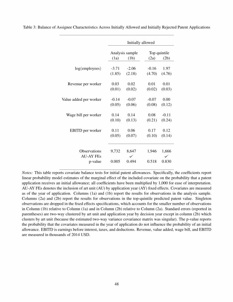
Table 3: Balance of Assignee Characteristics Across Initially Allowed and Initially Rejected Patent Applications

Initially allowed

Analysis sample Top quintile(1a) (1b) (2a) (2b)

log(employees) -3.71 -2.06 -0.16 1.97(1.85) (2.18) (4.70) (4.76)

Revenue per worker 0.03 0.02 0.01 0.01(0.01) (0.02) (0.02) (0.03)

Value added per worker -0.14 -0.07 -0.07 0.00(0.05) (0.06) (0.08) (0.12)

Wage bill per worker 0.14 0.14 0.08 -0.11(0.10) (0.13) (0.21) (0.24)

EBITD per worker 0.11 0.06 0.17 0.12(0.05) (0.07) (0.10) (0.14)

Observations 9,732 8,647 1,946 1,666AU-AY FEs

p-value 0.005 0.494 0.518 0.830

Notes: This table reports covariate balance tests for initial patent allowances. Specifically, the coefficients reportlinear probability model estimates of the marginal effect of the included covariate on the probability that a patentapplication receives an initial allowance; all coefficients have been multiplied by 1,000 for ease of interpretation.AU-AY FEs denotes the inclusion of art unit (AU) by application year (AY) fixed effects. Covariates are measuredas of the year of application. Columns (1a) and (1b) report the results for observations in the analysis sample.Columns (2a) and (2b) report the results for observations in the top-quintile predicted patent value. Singletonobservations are dropped in the fixed effects specifications, which accounts for the smaller number of observationsin Column (1b) relative to Column (1a) and in Column (2b) relative to Column (2a). Standard errors (reported inparentheses) are two-way clustered by art unit and application year by decision year except in column (2b) whichclusters by art unit (because the estimated two-way variance covariance matrix was singular). The p-value reportsthe probability that the covariates measured in the year of application do not influence the probability of an initialallowance. EBITD is earnings before interest, taxes, and deductions. Revenue, value added, wage bill, and EBITDare measured in thousands of 2014 USD.

48

Table 4: Prediction of KPSS Patent Value Based on Patent Application and Assignee Characteristics

KPSS value (ξ )

1(patent family size = 1) 0.28 (0.06)

log(patent family size) 0.23 (0.04)

1(number of claims = 1) 0.68 (0.19)

log(number of claims) 0.30 (0.03)

1(revenue = 0) 1.42 (0.14)

log(revenue) 0.14 (0.02)

1(employees = 0) 0.45 (0.07)

log(employees) -0.01 (0.02)

Application year -0.03 (0.05)

(Application year)2 -0.01 (0.01)

Decision year 0.30 (0.06)

(Decision year)2 -0.03 (0.01)

Constant -1.40 (0.21)

log(σ) 0.24 (0.05)

Observations 596Art units 260

χ2 10,353

Notes: This table reports the relationship between KPSS ξ patent value, and patent application and firm level co-variates. Coefficient estimates are from a Poisson model with art unit random effects. The sample is the subsampleof granted patents for which the Kogan et al. (2017) measure of patent value is available in our analysis sample,except we retain firms with more than 100 million in 2014 revenue (unlike in our analysis sample) in order tomaximize sample size (N=596). The dependent variable is the KPSS measure of patent value ξ in millions of1982 dollars. Standard errors are reported in parentheses. Patent family size measures the number of countries inwhich the patent application was submitted. Number of claims measures the number of claims in the published USpatent application. Revenue (in thousands of 2014 dollars) and number of employees are measured as of the yearthe US patent application was filed. log(σ ) reports the log of the estimated variance of the art unit random effects.χ2 reports the results of a likelihood ratio test statistic against a restricted Poisson model without art unit randomeffects; this test has one degree of freedom.

49

Tabl

e5:

Impa

cts

onFi

rmA

ggre

gate

s

(1)

(2)

(3)

(4)

(5)

(6)

(7)

(8)

(9)

(10)

Posi

tive

empl

oy-

men

tL

ogfir

msi

ze

Rev

enue

per

wor

ker

Val

uead

ded

per

wor

ker

EB

ITD

per

wor

ker

Wag

ebi

llpe

rw

orke

r

Surp

lus

per

wor

ker

Lab

orco

mp

per

wor

ker

W2

+10

99pe

rw

orke

r

Inco

me

tax

per

wor

ker

Pane

lA:a

llfir

ms

Hig

hva

lue

(Q5)

0.00

0.22

36.7

515

.74

9.11

3.65

12.4

13.

942.

800.

77(0

.04)

(0.0

9)(1

4.92

)(5

.25)

(3.8

3)(1

.55)

(3.5

6)(2

.79)

(1.5

3)(0

.68)

Mea

nof

outc

ome

(Q5)

0.69

2.84

286.

0011

0.70

9.07

52.4

962

.72

51.2

545

.48

16.1

1%

Impa

ct(Q

5)-0

.612

.814

.210

0.4

7.0

19.8

7.7

6.2

4.8

Low

erva

lue

(<Q

5)0.

000.

03-9

.68

0.84

-1.4

20.

80-0

.26

1.32

0.52

0.74

(0.0

1)(0

.04)

(8.4

0)(3

.82)

(1.7

7)(0

.90)

(2.0

5)(1

.65)

(0.8

6)(0

.56)

Obs

erva

tions

155,

646

103,

437

103,

437

103,

437

103,

437

103,

437

103,

437

103,

437

107,

789

103,

159

Pane

lB:c

lose

lyhe

ldfir

ms

Hig

hva

lue

(Q5)

-0.0

40.

3379

.75

32.7

221

.84

8.49

31.1

17.

135.

172.

21(0

.08)

(0.1

4)(2

4.60

)(8

.24)

(6.0

8)(3

.42)

(7.4

4)(1

.38)

(1.9

8)(1

.64)

Mea

nof

outc

ome

(Q5)

0.70

2.80

283.

8011

1.80

18.6

746

.47

66.1

744

.22

40.5

316

.34

%Im

pact

(Q5)

-5.2

28.1

29.3

117.

018

.347

.016

.112

.813

.6

Low

erva

lue

(<Q

5)-0

.02

0.02

-3.2

9-0

.70

0.71

0.30

0.53

0.34

-0.1

11.

23(0

.02)

(0.0

5)(1

3.95

)(6

.19)

(3.1

9)(1

.51)

(4.0

3)(2

.55)

(1.4

1)(1

.07)

Obs

erva

tions

75,1

3249

,943

49,9

4349

,943

49,9

4349

,943

49,9

4349

,943

51,9

9849

,808

Not

es:

Thi

sta

ble

repo

rts

diff

eren

ce-i

n-di

ffer

ence

ses

timat

esof

the

effe

ctof

initi

alpa

tent

allo

wan

ces

onfir

man

dw

orke

rou

tcom

es,

sepa

rate

lyfo

rhi

ghan

dlo

wex

-ant

eva

luab

lepa

tent

appl

icat

ions

,in

our

anal

ysis

sam

ple.

Pane

lBre

plic

ates

Pane

lA,b

utre

stri

cts

the

anal

ysis

toS-

corp

orat

ions

and

part

ners

hips

(“cl

osel

yhe

ld”

firm

s).

Est

imat

esco

rres

pond

toco

effic

ient

son

inte

ract

ions

ofth

ede

sign

ated

valu

eca

tego

ryw

itha

post

-dec

isio

nin

dica

tor

and

anin

dica

torf

orth

eap

plic

atio

nbe

ing

initi

ally

allo

wed

.Con

trol

sin

clud

em

ain

effe

ctof

valu

eca

tego

ryin

tera

cted

with

apo

st-d

ecis

ion

indi

cato

r,fir

mfix

edef

fect

s,an

dar

tuni

tby

appl

icat

ion

year

byca

lend

arye

arfix

edef

fect

s,as

ineq

uatio

n(8

).St

anda

rder

rors

(rep

orte

din

pare

nthe

ses)

are

two-

way

clus

tere

dby

(1)a

rtun

it,an

d(2

)app

licat

ion

year

byde

cisi

onye

ar.P

anel

Bdo

cum

ents

impa

cts

oncl

osel

yhe

ldfir

ms.

EB

ITD

isea

rnin

gsbe

fore

inte

rest

,ta

xes,

and

dedu

ctio

ns.

Surp

lus

isE

BIT

D+

wag

ebi

ll.L

abor

com

pens

atio

nm

easu

res

tota

lded

uctio

nsfo

rla

bor

expe

nses

clai

med

byth

efir

m.

“W2

+10

99”

mea

sure

sto

the

sum

ofW

2an

d10

99ea

rnin

gsdi

vide

dby

the

sum

ofth

enu

mbe

rofW

2’s

and

1099

’sfil

ed.“

Inco

me

tax

perw

orke

r”is

the

aver

age

wor

ker’

sin

divi

dual

inco

me

tax

liabi

lity.

Rev

enue

,val

uead

ded,

EB

ITD

,wag

ebi

ll,su

rplu

s,la

bor

com

pens

atio

n,an

dW

2+

1099

pay

are

repo

rted

inth

ousa

nds

of20

14U

SD.

50

Tabl

e6:

Wor

kfor

ceC

ompo

sitio

n

(1)

(2)

(3)

(4)

(5)

(6)

(7)

(8)

Shar

efe

mal

eSh

are

inve

ntor

s

Avg

entr

ant

earn

ings

(yrb

efen

t)

Avg

sepa

rato

rea

rnin

gs(y

rbef

sep)

Avg

stay

erea

rnin

gs(i

nap

pyr

)A

vgag

eL

ogqu

ality

Log

qual

ity(e

xpan

ded)

Hig

hva

lue

(Q5)

-0.0

1-0

.01

-0.8

40.

721.

29-1

.10

-0.0

2-0

.01

(0.0

1)(0

.01)

(2.0

5)(1

.11)

(1.5

8)(0

.56)

(0.0

3)(0

.03)

Mea

nof

outc

ome

(Q5)

0.31

0.09

24.4

228

.19

66.5

941

.74

10.4

310

.56

%Im

pact

(Q5)

-1.9

-12.

5-3

.42.

61.

9-2

.6-0

.2-0

.1

Low

erva

lue

(<Q

5)-0

.01

-0.0

10.

490.

001.

010.

080.

00-0

.01

(0.0

1)(0

.01)

(0.7

0)(0

.53)

(1.1

9)(0

.22)

(0.0

1)(0

.01)

Obs

erva

tions

103,

437

103,

437

70,0

7975

,524

99,5

5810

3,43

410

3,43

797

,786

Not

es:

Thi

sta

ble

repo

rts

diff

eren

ce-i

n-di

ffer

ence

ses

timat

esof

the

effe

ctof

initi

alpa

tent

allo

wan

ces

onw

ithin

-firm

wor

kfor

ceco

mpo

sitio

nm

easu

res,

sepa

rate

lyfo

rhi

ghan

dlo

wex

-ant

eva

luab

lepa

tent

appl

icat

ions

,in

our

anal

ysis

sam

ple.

Est

imat

esco

rres

pond

toco

effic

ient

son

inte

ract

ions

ofth

ede

sign

ated

valu

eca

tego

ryw

itha

post

-dec

isio

nin

dica

tor

and

anin

dica

tor

for

the

appl

icat

ion

initi

ally

allo

wed

.C

ontr

ols

incl

ude

mai

nef

fect

ofva

lue

cate

gory

inte

ract

edw

itha

post

-dec

isio

nin

dica

tor,

firm

fixed

effe

cts,

and

artu

nitb

yap

plic

atio

nye

arby

cale

ndar

year

fixed

effe

cts,

asin

equa

tion

(8).

Stan

dard

erro

rs(r

epor

ted

inpa

rent

hese

s)ar

etw

o-w

aycl

uste

red

by(1

)ar

tuni

t,an

d(2

)ap

plic

atio

nye

arby

deci

sion

year

.“A

vgen

tran

tear

ning

s(y

rbe

fen

t)”

mea

sure

sth

eea

rnin

gsof

entr

ants

inth

eye

arbe

fore

they

join

edth

efir

m.“

Avg

sepa

rato

rear

ning

s(y

rbef

sep)

”m

easu

res

the

earn

ings

ofse

para

tors

inth

eye

arbe

fore

they

leav

eth

efir

m.S

taye

rsar

ede

fined

asth

ose

who

wer

eem

ploy

edby

the

sam

efir

min

the

year

ofap

plic

atio

n.E

ntra

nts

are

defin

edas

thos

eem

ploy

ees

who

wer

eno

tem

ploy

edat

the

firm

inth

epr

evio

usye

ar.“

Avg

age”

mea

sure

sth

eav

erag

eag

eof

alle

mpl

oyee

sat

the

firm

.Ear

ning

sar

em

easu

red

inth

ousa

nds

of20

14U

SD.“

Log

qual

ity”

give

spr

edic

ted

log

wag

eba

sed

onw

orke

rde

mog

raph

ics

and

inve

ntor

stat

us.

“Log

qual

ity(e

xpan

ded)

”in

clud

esw

age

onpr

evio

usjo

bin

pred

ictiv

em

odel

.See

text

ford

etai

ls.

51

Tabl

e7:

Ear

ning

sIm

pact

sby

Yea

rofE

ntry

/Exi

t

Cha

nge

sinc

eap

plic

atio

nye

ar

(1)

(2)

(3)

(4)

(5)

(6)

(7)

(8)

Avg

coho

rtea

rnin

gs

Avg

stay

erea

rnin

gs

Avg

leav

erea

rnin

gs

Avg

entr

ant

earn

ings

Avg

rece

nten

tran

tea

rnin

gs

Avg

stay

erea

rnin

gs

Avg

leav

erea

rnin

gs

Avg

entr

ant

earn

ings

Hig

hva

lue

(Q5)

3.96

7.78

-1.5

40.

11-2

.71

6.50

2.77

0.95

(2.2

9)(2

.93)

(1.9

4)(1

.64)

(1.8

1)(3

.10)

(5.6

5)(1

.80)

Mea

nof

outc

ome

(Q5)

57.3

972

.56

50.5

730

.13

38.9

372

.56

50.5

730

.13

%Im

pact

(Q5)

6.9

10.7

-3.0

0.4

-7.0

9.0

5.5

3.2

Low

erva

lue

(<Q

5)0.

342.

480.

900.

310.

781.

48-3

.87

-0.1

8(1

.18)

(1.5

9)(1

.39)

(0.7

9)(1

.01)

(1.6

3)(2

.40)

(0.7

0)

Obs

erva

tions

151,

892

99,5

5810

9,16

970

,079

68,6

9199

,558

109,

169

70,0

79

Not

es:

Thi

sta

ble

repo

rts

diff

eren

ce-i

n-di

ffer

ence

ses

timat

esof

the

effe

ctof

initi

alpa

tent

allo

wan

ces

onw

orke

rout

com

esfo

rem

ploy

ees

who

stay

,ent

er,

and

exit

ξ̂,

sepa

rate

lyfo

rhi

ghan

dlo

wex

-ant

eva

luab

lepa

tent

appl

icat

ions

.E

stim

ates

corr

espo

ndto

coef

ficie

nts

onin

tera

ctio

nsof

the

desi

gnat

edva

lue

cate

gory

with

apo

st-d

ecis

ion

indi

cato

rand

anin

dica

torf

orth

eap

plic

atio

nbe

ing

initi

ally

allo

wed

.Con

trol

sin

clud

em

ain

effe

ctof

valu

eca

tego

ryin

tera

cted

with

apo

st-d

ecis

ion

indi

cato

r,fir

mfix

edef

fect

s,an

dar

tuni

tby

appl

icat

ion

year

byca

lend

arye

arfix

edef

fect

s,as

ineq

uatio

n(8

).St

anda

rder

rors

(rep

orte

din

pare

nthe

ses)

are

two-

way

clus

tere

dby

(1)

artu

nit,

and

(2)

appl

icat

ion

year

byde

cisi

onye

ar.

“Avg

coho

rtea

rnin

gs”

mea

sure

sth

eW

2ea

rnin

gsof

wor

kers

empl

oyed

byth

efir

min

the

year

ofap

plic

atio

n.“A

vgst

ayer

earn

ings

”m

easu

res

the

W2

earn

ings

ofw

orke

rsem

ploy

edby

the

firm

inth

eye

arof

appl

icat

ion

who

are

also

empl

oyed

inth

epr

esen

tyea

r.“A

vgle

aver

earn

ings

”m

easu

res

the

W2

earn

ings

ofw

orke

rsem

ploy

edby

the

firm

inth

eye

arof

appl

icat

ion

who

are

note

mpl

oyed

inth

epr

esen

tyea

r.“A

vgen

tran

tear

ning

s”m

easu

res

the

W2

earn

ings

ofem

ploy

ees

who

wer

eno

tem

ploy

edby

the

firm

inth

epr

evio

usye

ar.“

Avg

rece

nten

tran

tear

ning

s”tr

acks

the

aver

age

earn

ings

ofem

ploy

ees

hire

dby

the

firm

with

inth

epa

stth

ree

year

s.“C

hang

esi

nce

appl

icat

ion

year

”co

lum

nsar

eea

rnin

gsin

the

curr

enty

ear(

Col

umns

6an

d7)

,and

year

ofen

try

(Col

umn

8)m

inus

the

resp

ectiv

eva

lues

inth

eap

plic

atio

nye

ar.S

taye

rsar

ede

fined

asth

ose

who

wer

eem

ploy

edby

the

sam

efir

min

the

year

ofap

plic

atio

n.E

ntra

nts

are

defin

edas

thos

eem

ploy

ees

who

wer

eno

tem

ploy

edat

the

firm

inth

epr

evio

usye

ar.E

arni

ngs

are

mea

sure

din

thou

sand

sof

2014

USD

.

52

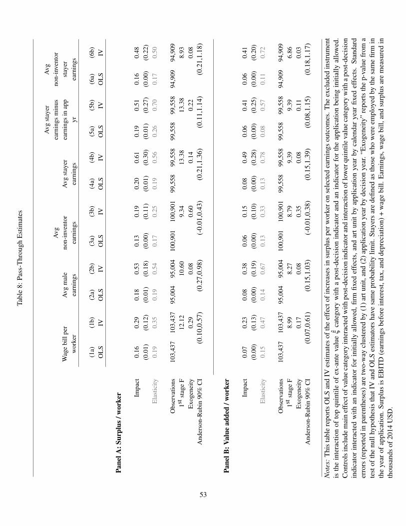
Tabl

e8:

Pass

-Thr

ough

Est

imat

es

Wag

ebi

llpe

rw

orke

rA

vgm

ale

earn

ings

Avg

non-

inve

ntor

earn

ings

Avg

stay

erea

rnin

gs

Avg

stay

erea

rnin

gsm

inus

earn

ings

inap

pyr

Avg

non-

inve

ntor

stay

erea

rnin

gs

(1a)

(1b)

(2a)

(2b)

(3a)

(3b)

(4a)

(4b)

(5a)

(5b)

(6a)

(6b)

OL

SIV

OL

SIV

OL

SIV

OL

SIV

OL

SIV

OL

SIV

Pane

lA:S

urpl

us/w

orke

r Impa

ct0.

160.

290.

180.

530.

130.

190.

200.

610.

190.

510.

160.

48(0

.01)

(0.1

2)(0

.01)

(0.1

8)(0

.00)

(0.1

1)(0

.01)

(0.3

0)(0

.01)

(0.2

7)(0

.00)

(0.2

2)E

last

icity

0.19

0.35

0.19

0.54

0.17

0.25

0.19

0.56

0.26

0.70

0.17

0.50

Obs

erva

tions

103,

437

103,

437

95,0

0495

,004

100,

901

100,

901

99,5

5899

,558

99,5

5899

,558

94,9

0994

,909

1st s

tage

F12

.12

10.6

09.

3413

.38

13.3

88.

93E

xoge

neity

0.29

0.08

0.60

0.14

0.22

0.08

And

erso

n-R

ubin

90%

CI

(0.1

0,0.

57)

(0.2

7,0.

98)

(-0.

01,0

.43)

(0.2

1,1.

36)

(0.1

1,1.

14)

(0.2

1,1.

18)

Pane

lB:V

alue

adde

d/w

orke

r

Impa

ct0.

070.

230.

080.

380.

060.

150.

080.

490.

060.

410.

060.

41(0

.00)

(0.1

3)(0

.00)

(0.1

9)(0

.00)

(0.1

0)(0

.00)

(0.2

8)(0

.00)

(0.2

5)(0

.00)

(0.2

0)E

last

icity

0.15

0.47

0.14

0.67

0.13

0.33

0.13

0.78

0.08

0.57

0.11

0.72

Obs

erva

tions

103,

437

103,

437

95,0

0495

,004

100,

901

100,

901

99,5

5899

,558

99,5

5899

,558

94,9

0994

,909

1st s

tage

F8.

998.

278.

799.

399.

396.

86E

xoge

neity

0.17

0.08

0.35

0.08

0.11

0.03

And

erso

n-R

ubin

90%

CI

(0.0

7,0.

61)

(0.1

5,1.

03)

(-0.

01,0

.38)

(0.1

5,1.

39)

(0.0

8,1.

15)

(0.1

8,1.

17)

Not

es:

Thi

sta

ble

repo

rts

OL

San

dIV

estim

ates

ofth

eef

fect

ofin

crea

ses

insu

rplu

spe

rwor

kero

nse

lect

edea

rnin

gsou

tcom

es.T

heex

clud

edin

stru

men

tis

the

inte

ract

ion

ofto

pqu

intil

eof

ex-a

nte

valu

eξ̂

cate

gory

with

apo

st-d

ecis

ion

indi

cato

ran

dan

indi

cato

rfo

rth

eap

plic

atio

nbe

ing

initi

ally

allo

wed

.C

ontr

olsi

nclu

dem

ain

effe

ctof

valu

eca

tego

ryin

tera

cted

with

post

-dec

isio

nin

dica

tora

ndin

tera

ctio

nof

low

erqu

intil

eva

lue

cate

gory

with

apo

st-d

ecis

ion

indi

cato

rin

tera

cted

with

anin

dica

tor

for

initi

ally

allo

wed

,firm

fixed

effe

cts,

and

artu

nitb

yap

plic

atio

nye

arby

cale

ndar

year

fixed

effe

cts.

Stan

dard

erro

rs(r

epor

ted

inpa

rent

hese

s)ar

etw

o-w

aycl

uste

red

by(1

)art

unit,

and

(2)a

pplic

atio

nye

arby

deci

sion

year

.“E

xoge

neity

”re

port

sth

ep-

valu

efr

oma

test

ofth

enu

llhy

poth

esis

that

IVan

dO

LS

estim

ator

sha

vesa

me

prob

abili

tylim

it.St

ayer

sar

ede

fined

asth

ose

who

wer

eem

ploy

edby

the

sam

efir

min

the

year

ofap

plic

atio

n.Su

rplu

sis

EB

ITD

(ear

ning

sbe

fore

inte

rest

,tax

,and

depr

ecia

tion)

+w

age

bill.

Ear

ning

s,w

age

bill,

and

surp

lus

are

mea

sure

din

thou

sand

sof

2014

USD

.

53

Tabl

e9:

Ret

entio

nof

appl

icat

ion

coho

rt

(1)

(2)

(3)

(4)

(5)

All

Abo

vem

edia

nM

enW

omen

Non

-inv

ento

rs

Ret

entio

nel

astic

ity1.

221.

410.

801.

171.

31(0

.58)

(0.6

5)(0

.35)

(0.8

0)(0

.68)

Sepa

ratio

nel

astic

ity-1

.74

-2.9

1-1

.23

-1.8

8-1

.79

Obs

erva

tions

99,5

5881

,728

88,1

0071

,591

94,9

091s

t sta

geF

7.81

5.80

31.1

33.

616.

74E

xoge

neity

0.03

40.

029

0.04

10.

060

0.04

7A

nder

son-

Rub

in90

%C

I(0

.459

,3.0

80)

(0.5

97,4

.091

)(0

.283

,1.5

24)

(0.2

33,8

.687

)(0

.422

,3.6

55)

Not

es:

Thi

sta

ble

repo

rts

IVes

timat

esof

the

effe

ctof

incr

ease

sin

sele

cted

earn

ings

mea

sure

son

the

rete

ntio

nof

empl

oyee

s.T

heex

clud

edin

stru

men

tis

the

inte

ract

ion

ofto

pqu

intil

eof

ex-a

nte

valu

eξ̂

cate

gory

with

apo

st-d

ecis

ion

indi

cato

ran

dan

indi

cato

rfo

rth

eap

plic

atio

nbe

ing

initi

ally

allo

wed

.C

ontr

olsi

nclu

dem

ain

effe

ctof

valu

eca

tego

ryin

tera

cted

with

post

-dec

isio

nin

dica

tora

ndin

tera

ctio

nof

low

erqu

intil

eva

lue

cate

gory

with

apo

st-d

ecis

ion

indi

cato

rin

tera

cted

with

anin

dica

tor

for

initi

ally

allo

wed

,firm

fixed

effe

cts,

and

artu

nitb

yap

plic

atio

nye

arby

cale

ndar

year

fixed

effe

cts.

Stan

dard

erro

rs(r

epor

ted

inpa

rent

hese

s)ar

etw

o-w

aycl

uste

red

by(1

)ar

tun

it,an

d(2

)ap

plic

atio

nye

arby

deci

sion

year

.“S

epar

atio

nel

astic

ity”

repo

rts

the

elas

ticity

ofth

eou

tcom

ere

tent

ion

mea

sure

with

resp

ectt

oth

eas

soci

ated

earn

ings

mea

sure

atth

em

ean

ofth

eou

tcom

ean

dth

em

ean

earn

ings

mea

sure

.“E

xoge

neity

”re

port

sp-

valu

efo

rtes

tofn

ullh

ypot

hesi

sth

atIV

and

OL

Ses

timat

ors

have

sam

epr

obab

ility

limit.

“Abo

vem

edia

n”re

fers

tom

embe

rsof

the

appl

icat

ion

coho

rtw

hoea

rned

abov

eth

atfir

m’s

med

ian

inth

eap

plic

atio

nye

ar.S

taye

rsar

ede

fined

asth

ose

who

wer

eem

ploy

edby

the

sam

efir

min

the

year

ofap

plic

atio

n.E

arni

ngs

are

mea

sure

din

thou

sand

sof

2014

USD

.

54

A Appendix: Data

A.1 Description of patent data

Our patent data build draws on several sources. Three identification numbers are relevant when using thesedatasets. First, publication numbers are unique identifiers assigned to published patent applications. Second,application numbers are unique identifiers assigned to patent applications that in practice are quite similar topublication numbers, but sometimes one application number is associated with multiple publication numbers.Finally, patent grant numbers are unique identifiers assigned to granted patents. Note that one patent applicationnumber can be associated with more than one granted patent.

Traditionally, unsuccessful patent applications were not published by the USPTO. However, as part of theAmerican Inventors Protection Act of 1999, the vast majority of patent applications filed in the US on or after 29November 2000 are published eighteen months after the filing date. There are two exceptions. First, applicationsgranted or abandoned before eighteen months do not appear in this sample unless the applicant chooses to askfor early publication. Lemley and Sampat (2008) estimate that about 17 percent of patents are granted beforeeighteen months, of which about half (46 percent) are published pre-patent grant. Second, applications pendingmore than eighteen months can “opt out" of publication if they do not have corresponding foreign applications, orif they have corresponding foreign applications but also have priority dates predating the effective date of the lawrequiring publication (Lemley, and Sampat 2008).29

1. Census of published USPTO patent applications. We observe the census of published (accepted and rejected)patent applications published by the US Patent and Trademark Office (USPTO). Our source for this data is aset of bulk XML files hosted by Google.30 The underlying XML file formats were often inconsistent acrossyears, so in the process of parsing these XML files to flat files we attempted to validate the data against otherUSPTO administrative data wherever possible. These records are at the publication number level.

2. Census of granted USPTO patents. For the published USPTO patent applications in our data, we wish toobserve which of those applications were granted patents. Our source for this data is a set of bulk XMLfiles hosted by Google.31 As with the published USPTO patent applications data, the underlying XML fileformats were often inconsistent across years, so in the process of parsing these XML files to flat files weattempted to validate the data against other USPTO administrative data wherever possible. As one specificexample, even though patent numbers uniquely identify patent grants, there are twenty-one patent numbersin this data that appear in the data twice with different grant dates. Checking these patent numbers on theUSPTO’s online Patent Full Text (PatFT) database reveals that in each of these cases, the duplicated patentnumber with the earlier grant date is correct.32 Accordingly, we drop the twenty-one observations with thelater grant dates.

3. USPTO patent assignment records. Some of our published patent applications are missing assignee informa-tion. (Applicants are not required to submit assignee information to the USPTO at the time of application.)Based on informal conversations with individuals at the USPTO, we fill in missing assignee names to theextent possible using the USPTO Patent Assignment data. The USPTO Patent Assignment data records as-signment transactions, which are legal transfers of all or part of the right, title, and interest in a patent orapplication from one or more existing owner to one or more recipient. The dataset is hosted on the USPTO

29For more details, see http://www.uspto.gov/web/offices/pac/mpep/s1120.html and the discussion in Lemley and Sampat(2010). Most applications not published eighteen months after filing are instead published sixty months after filing.

30See http://www.google.com/googlebooks/uspto-patents-applications-biblio.html.31See http://www.google.com/googlebooks/uspto-patents-grants-text.html.32PatFT can be accessed at http://patft.uspto.gov/.

55

website.33 Each transaction is associated with a patent number, application number, and/or publicationnumber (wherever each is applicable). The patent assignment records include both initial assignments andre-assignments, but only the former is conceptually appropriate for our analysis since we want to measureinvention ownership at the time of application. We isolate initial assignments by taking the assignment fromthis database with the earliest execution date. If a given assignment has more than one execution date (e.g.,if the patent application is assigned to more than one entity), we use the latest execution date within thatassignment as the transaction execution date. Using these initial assignments, we fill in assignee organiza-tion name as well as assignee address information where possible when these variables are missing from ourpublished patent applications data.

4. USPTO patent document pre-grant authority files. A very small number (1,025 total) of published USPTOpatent applications are “withdrawn,” and these observations tend to be inconsistently reported across thevarious datasets we analyze. The USPTO patent document pre-grant authority files — an administrativedata file hosted on the USPTO website — allows us to exclude all withdrawn applications for consistency.34

Our versions of these files were downloaded on 24 March 2014 and are up to date as of February 2014.These records are at the publication number level.

5. USPTO PAIR records. We analyze several variables, such as the date of initial decisions, from the USPTOPatent Application Information Retrieval (PAIR) data, which we draw from an administrative dataset calledthe Patent Examination Research Dataset (PatEx).35 With the exception of 264 published patent applications,these data are available for our full sample of published USPTO patent applications. These records are at theapplication number level.

6. Examiner art unit and pay scale data. Frakes and Wasserman (2017) generously provided us with examinerart unit and General Schedule (GS) pay scale data they received through FOIA requests. These data allowus to identify which examiners were active in each art unit in each year.

7. Thomson Innovation database. All of the databases listed above record information obtained directly fromthe USPTO. One measure of patent value that cannot be constructed based on the USPTO records alone isa measure of patent family size, as developed in Jonathan Putnam’s dissertation (Putnam 1996). Generallystated, a patent “family” is defined as a set of patent applications filed with different patenting authorities(e.g., the US, Europe, Japan) that refer to the same invention. The key idea is that if there is a per-countrycost of filing for a patent, firms will be more likely to file a patent application in multiple countries ifthey perceive the patent to have higher private value. Past work — starting with Putnam (1996) — hasdocumented evidence that patent family size is correlated with other measures of patent value. The ThomsonReuters Innovation database collects non-US patent records, and hence allows for the construction of such afamily size measure.36 We purchased a subscription to the Thomson Innovation database, and exported datafrom the web interface on all available variables for all published USPTO patent applications. To constructour family size measure, we take the DWPI family variable available in the Thomson Innovation database(which lists family members), separate the country code from the beginning of each number (e.g., “US” in“US20010003111”), and then count the number of unique country codes in the family. These records are atthe publication number level.

8. Hall, Jaffe, and Trajtenberg (2001) NBER data. Hall, Jaffe, and Trajtenberg (2001) constructed a matchbetween US patents granted between January 1963 and December 1999 with the Compustat data. As part

33Available at: https://www.uspto.gov/learning-and-resources/electronic-data-products/patent-assignment-dataset.

34See http://www.uspto.gov/patents/process/search/authority/.35See http://www.uspto.gov/learning-and-resources/electronic-data-products/patent-examination-research-dataset-public-pair;

for the underlying PAIR data, see: http://portal.uspto.gov/pair/PublicPair.36See http://info.thomsoninnovation.com/.

56

of that work, the authors constructed technology categories to describe the broad content area of differentpatents, based on categorizations of the patent technology class and subclass variables.37 We match on thesetechnology categories, and hand-fill the small number of cases in which classes or subclasses appear in ourdata but not in the crosswalk constructed by Hall and co-authors. These records are at the patent class level.

9. Kogan et al. (2017) patent value data. Kogan et al. (2017) provide their final estimates of patent value fortheir sample of granted patents at https://iu.app.box.com/v/patents/. In particular we downloadedthe “patents.zip” file, which contains a linkage between USPTO patent grant numbers and the estimate ofthe patent value ξ . These data were downloaded on — and are accurate as of — 7 August 2016. To developa measure of patent value at the application number level, we associate each application with its potentiallynumerous patent numbers. We then sum the values of ξ by application number to obtain a measure of theex-post value of granted applications.

10. USPTO technology center data. Technology centers are groupings of examiner art units. The USPTOhosts a listing of all technology centers and associated examiner art units at http://www.uspto.gov/patent/contact-patents/patent-technology-centers-management. We use these groupings to ex-amine heterogeneity in predicted patent value by area of invention in Appendix Table C.2.

A.2 Construction of patent application sample

We restrict the sample to USPTO patent applications filed on or after 29 November 2000 (the date when“rejected” applications started to be published), and ends with applications published on 31 December 2013. Weimpose a few additional sample restrictions:

• We exclude a very small number of “withdrawn” patent applications (1,025 total) given that these observa-tions tend to be inconsistently reported across datasets. As noted above, the withdrawn applications wereidentified using the USPTO patent document pre-grant authority files.

• Six publication numbers are listed in the USPTO patent document pre-grant authority files but are not avail-able in any of our other datasets;38 we exclude these observations from our sample.

• Four publication numbers are missing from the Thomson Innovation database.39 We include these observa-tions in the sample, but they are missing data for all variables drawn from the Thomson Innovation data.

• Based on the kind code variable listed on the USPTO published patent applications,40 we exclude a smallnumber of patent applications that are corrections of previously published applications: corrections of pub-lished utility/plant patent applications (kind codes A9/P9; 3,156 total), and second or subsequent publica-tions of the same patent application (kind codes A2/P4; 1,182 total). These kind codes more generally allowus to confirm that our sample does not include various types of documents: statutory invention registrationdocuments (kind code H1), reexamination certificates (kind codes Bn/Cn/Fn for n=1-9), post grant reviewcertificates (kind codes Jn for n=1-9), inter parties review certificates (kind codes Kn for n=1-9), or deriva-tion certificates (kind codes On for n=1-9). Our final sample includes only utility patent applications (kindcode A1; 3,597,787 total) and plant patent applications (kind code P1; 4,196 total).

Finally, there are two data inconsistencies that we have resolved as follows:

37See http://www.nber.org/patents/.38Specifically, these publication numbers are: US20010003111; US20020011585; US20020054271; US20020084413; US20020084764;

and US20020103782.39Specifically, these publication numbers are: US20010020331; US20010020666; US20010021099; and US20010021102.40For a summary of USPTO kind codes, see: http://www.uspto.gov/patents/process/search/authority/kindcode.jsp.

57

• Seven observations appear to be missing from Google’s XML files of the published patent applications.41 Wewere able to hand-code the required variables for these observations based on the published patent applica-tions posted at http://patft.uspto.gov for all but three of these observations (specifically, publicationnumbers US20020020603; US20020022313; US20020085735). For those three observations, we hand-coded the required variables based on the information available at http://portal.uspto.gov/pair/PublicPair/; for these, we assumed that the appropriate correspondent addresses were those listed inthe “Address and Attorney/Agent” field under Correspondence Address.

• The applications data contain 67 applications that were approved SIR (statutory invention registration) statusbut have the kind code “A1,” instead of “H1” (as we would expect). We changed the kind code to “H1” forthese applications, and they are therefore dropped from our sample.

A.3 Description of US Treasury tax files

All firm-level variables are constructed from annual business tax returns over the years 1997-2014: C-Corporations(Form 1120), S-Corporations (Form 1120S), and Partnerships (Form 1065). Worker-level variables are constructedfrom annual tax returns over the years 1999–2014: Employees (form W2) and contractors (form 1099).42

Variable Definitions

To define firm-level variables using the US Treasury files, we use the following line items from the 2010business tax forms: 1120 for C-corporations, 1120S for S-corporations, and 1065 for partnerships. Note that thetax form line numbers can sometimes change slightly if, for example, a line is added for a new deduction.

• Revenue

– Line 1c of Form 1120 for C-Corporations, Form 1120S for S-Corporations, and Form 1065 for part-nerships. When 1c is not available, we use 1a, which is gross receipts. We replace negative revenueentries, which are very rare, with missing values.

• Total Income

– For C-Corporations, line 11 on Form 1120. Note that this subtracts COGS from revenues and includesincome from a variety of sources (e.g., dividends, royalties, capital gains, etc). For S-Corporations,line 6 on Form 1120S. For partnerships, line 8 on Form 1065.

• Total Deductions

– For C-corporations, line 27 on Form 1120. For S-corporations, line 20 on Form 1120S. For partner-ships, line 21 on Form 1065.

• Labor Compensation

– For C-Corporations, sum of lines 12, 13, 24, and 25 on Form 1120.43 For S-Corporations, sum oflines 7, 8, 17, and 18 for Form 1120S. For partnerships, sum of lines 9, 10, 18, and 19 on Form 1065.These lines are compensation to officers, salaries and wages, retirement plans, and employment benefitprograms, respectively.44

41Specifically, the missing publication numbers are: US20010020331; US20010020666; US20010021099; US20010021102;US20020020603; US20020022313; US20020085735.

42W2 data are not available in 1997–1999.43Ideally, we could also add Schedule A line 3, which is the cost of labor on the COGS Form 1125-A, but these data are not available.

However, the W2-based measure of compensation avoids this issue.44For partnerships, the compensation to officers term is called “Guaranteed payments to partners.”

58

• Value Added

– Gross receipts minus the difference between cost of goods sold and cost of labor.

– For C-Corporations, line 3 on Form 1120. For S-corporations, line 3 on Form 1120S. For partnerships,line 3 on Form 1065.45

• Profits

– Yagan (2015) defines operating profits as revenues less Costs of Goods Sold and deductions wheredeductions are total deductions other than compensation to officers, interest expenses, depreciation,and domestic production activities deduction. We do not add back compensation to officers.

– For C-Corporations, we define operating profits as the sum of lines 1c, 18, and 20, less the sum of 2and 27 on Form 1120. We set profits to missing if 1c, 18, 20,2, and 27 are all equal to zero.

– For S-Corporations, operating profits are the sum of lines 1c, 13, and 14 less the sum of 2 and 20 onForm 1120S.

– For partnerships, operating profits are the sum of lines 1c, 15, and 16c less the sum of 2 and 21 onForm 1065.

• EBITD

– EBITD is total income less total deductions (other than interest and depreciation).

– For C-Corporations, it is the sum of lines 11, 18, and 20, less 27 on Form 1120.

– For S-Corporations, it is the sum of lines 1c, 13, and 14 less 20 on Form 1120S.

– For partnerships, it is the sum of lines 1c, 15, and 16c less 21 on Form 1065.

• Employment

– Number of W2s associated with an Employer Identification Number (EIN).

• Wage bill per worker

– Sum of W2 box 1 payments divided by number of W2s for a given EIN.

• Surplus

– Sum of EBITD and Wage bill, which is the sum of W2 box 1 payments for a given EIN.

• Inventor earnings per inventor

– Wage bill per worker for workers who are identified as inventors by Bell et al. (2016).

• Cohort earnings per worker

– Wage bill per worker for workers who were employed at the firm in the year of application regardlessof whether or not they stay at the firm.

• Stayer earnings per worker

45Line 3 is calculated as line 1c minus line 2.

59

– Stayers are cohort earning per worker for the set of workers who are still at the firm.

• Leaver earnings per worker

– Leavers are cohort earning per worker for the set of workers in the initial cohort who are no longer atthe firm, i.e., are no longer receiving a W2 associated with the original firm that applied for a patent.

• Earnings Gap Q4-Q1

– Average earnings within quartile four and quartile one of a firm’s wage distribution.

• Separators

– The number of workers who left the EIN in the previous year.

• Entrants

– The number of workers who joined the EIN relative to the previous year.

• State

– Uses the state from the business’s filing address.

• Entity Type

– Indicator based on tax-form filing type.

• Industry

– NAICS codes are line 21 on Schedule K of Form 1120 for C-Corporations, line 2a Schedule B of Form1120S for S-Corporations, and Box A of Form 1065 for partnerships.

• Active Firm

– An active firms has non-zero and non-missing total income and non-missing total deductions.

60

A.3.1 Deflator to convert to 2014 USD

Table A.1: Deflator to convert to 2014 USD

Year 1 / 2014 CPI Year 1 / 2014 CPI

1993 1.503062988 2004 1.2196638171994 1.47180133 2005 1.1816491821995 1.441698831 2006 1.1464160651996 1.415894851 2007 1.1166426961997 1.391942424 2008 1.0955068641998 1.377006398 2009 1.086941999 1.357571973 2010 1.0737755122000 1.327317133 2011 1.0520640762001 1.297761328 2012 1.0330165372002 1.278151458 2013 1.0164492452003 1.253173459 2014 1

Notes: This table shows the deflators used to convert our dollar amounts from current dollars into 2014 USD.Deflators were calculated using price data from BEA Table 1.1.4 (“Price Indexes for Gross Domestic Product”).

A.4 Description of merge between patent applications data and US Treasury tax files

Our analysis relies on a new merge between published patent applications submitted to the US Patent andTrademark Office (USPTO) and US Treasury tax files. Below we describe the details of this merge, which relieson a fuzzy matching algorithm to link USPTO assignee names with US Treasury firm names.

A.4.1 Creating standardized names within the patent data

Published patent applications list an assignee name, which reflects ownership of the patent application. Dueto, e.g., spelling differences, multiple assignee names in the USPTO published patent applications data can cor-respond to a single firm. For example, “ALCATEL-LUCENT U.S.A., INC.”, “ALCATEL-LUCENT USA, IN-CORPORATED,” and “ALCATEL-LUCENT USA INC” are all assigned the standardized name “alcatel lucentusa corp”.

We employed a name standardization routine as follows. Starting with names in unicode format, we transformthe text into Roman alphabet analogs using the “unidecode” library to map any foreign characters into their appli-cable English phonemes, and then shift all characters to lowercase.46 We then standardize common terms that takemultiple forms, such as “corp.” and “corporation”; these recodings were built on the name standardization routineused by the National Bureau of Economic Research (NBER)’s Patent Data Project, with modifications as we sawopportunities to improve that routine.47 We additionally eliminate any English articles (such as “a” or “an”), sincethese appeared to be uninformative in our attempts to uniquely identify entities. We then tokenize standardizednames by splitting on natural delimiters (e.g., spaces and commas), after which we remove any non-alphanumericpunctuation. Finally, sequences of single-character tokens are merged into a combined token (e.g., “3 m corp”

46The unidecode library is available at https://github/com/iki/unidecode, and is a direct Python port of the Text::Unidecode Perlmodule by Sean M. Burke.

47The NBER Patent Data Project standardization code is available at https://sites.google.com/site/patentdataproject/Home/posts/namestandardizationroutinesuploaded.

61

would become “3m corp”). The resultant ordered list of tokens constitutes our standardized entity name. We referto the USPTO standardized firm name as SNAMEUSPTO.

A.4.2 Creating standardized names within the US Treasury tax files

In the US Treasury tax files, firms are indexed by their Employer Identification Number (EIN). Each EIN isrequired to file a tax return for each year that it is in operation. Specifically, we restrict our analysis to firms withvalid 1120, 1120S, or 1065 filings over the years 1997–2014. We apply the same name standardization algorithmto the Treasury firm names that was applied to the USPTO names. We refer to the Treasury standardized firm nameas SNAMETreasury.

A.4.3 Merging standardized names across the USPTO data and the US Treasury tax files

We then conduct a fuzzy merge of SNAMEUSPTO to SNAMETreasury using the SoftTFIDF algorithm, which isdescribed below. We use this algorithm to allocate each SNAMEUSPTO to a single SNAMETreasury, provided thatmatch quality lies within a specified tolerance. To choose the tolerance we used a hand coded match of applicationsto Compustat firms as a validation dataset (see Section A.4.4). The tolerance (and other tuning parameters) werechosen to minimize the sum of Type I and II error rates associated with matches to Compustat firms. The resultingfirm-level dataset has one observation per SNAMETreasury in each year. However, there are some cases in whichmultiple EINs are associated with a given SNAMETreasury. In those cases, we chose the EIN with the largesttotal income in the year of application in order to select the most economically active entity associated with thatstandardized name.48

SoftTFIDF algorithm Our firm name matching procedure of name a∈ SNAMEUSPTO to name b∈ SNAMETreasury

works as follows. Among all the words in all the firm names in SNAMEUSPTO that are close to a given word in b,we pick the word with the highest SoftTFIDF index value, which is a word-frequency weighted measure of simi-larity among words. We do this for each word in the firm’s name. For instance, American Airlines Inc would havethree words. We then take a weighted-sum of the index value for each word in the firm name where the weightsare smaller for frequent words like "Inc." This weighted sum is the SoftTFIDF value at the level of firm-names(as opposed to words in firm names). We assign a to the firm name b with the highest SoftTFIDF value abovea threshold; otherwise, the name a is unmatched. Because of computational limitations, we limit comparisons tocases in which both a and b start with the same letter. Therefore we will miss any matches that do not share thesame first letter. This subsection provides details on this procedure and example matches.

SoftTFIDF of firm names A score between groups of words X ,Y is given by

SoftTFIDF(X ,Y ) := ∑w∈X

weight(w,X) ·α(w,Y )

where weight(w,X) is a word frequency-based importance weight and α(w,Y ) is a word match score that uses aword similarity index. Specifically, the importance weight for the word w in the set of words Z is: weight(w,Z) :=

tfidf(w,Z)√∑w′∈Z tfidf(w′,Z)2

, where

• tfidf(w,Z) := tf(w,Z)× idf(w,Z ),

• tf(w,Z) := n(w,Z)∑w′∈Z n(w′,Z) ,

• idf(w,Z ) := log(

|Z ||{Z∈Z | w∈Z}|

),

48For example, if two EINs shared the same standardized name SNAMETreasury but one EIN made 50 million in total income and theother showed three million in total income, we chose the EIN that earns 50 million.

62

• n(w,Z) is the number of occurrences of word w in a set of words Z,

• Z is the set of all words in either SNAMEUSPTO or SNAMEIRS.

We compute the word match score α(w,Y ) for words that are close to those in SNAMEUSPTO. To determine whichnames are close, we use a Jaro-Winkler distance metric to measure the distance between two strings.

Jaro-Winkler metric of distance between strings We use this metric since it has been shown to perform betterat name-matching tasks (Cohen, Ravikumar, and Fienburg 2003) than other metrics such as Levenshtein distance,which assigns unit cost to every edit operation (insertion, deletion, or substitution). A key component of theJaro-Winkler metric is the Jaro metric. The Jaro metric depends on the length of SNAMEUSPTO, the length ofSNAMETreasury, the number of shared letters, and the number of needed transpositions of shared letters.

Specifically, consider strings s = s1 . . .sK and t = t1 . . . tL and define H = min{|s|,|t|}2 , which is half the smaller of

K and L. We say a character si is in common with t if ∃ j ∈ [i−H, i+H] s.t. si = t j. Let s′, t ′ be the ordered setsof in-common characters (hence we will re-index). Then define Ts′,t ′ := 1

2 |{i | s′i 6= t ′i}|. The similarity metric isgiven by

Jaro(s, t) :=13·(|s′||s|

+|t ′||t|

+|s′|−Ts′,t ′

|s′|

).

The Jaro-Winkler metric is given by

Jaro-Winkler(s, t) := Jaro(s, t)+P′

10· (1− Jaro(s, t)),

where P as the longest common prefix of t and s and then P′ = max{P,4}, which is the normalization used inCohen, Ravikumar, and Fienburg (2003).

Word match score α(w,Z) We define the word match score as follows:

α(w,Z) =

0 if closest(θ ,w,Z) = /0max

w′∈closest(θ ,w,Z)weight(w′,Z) · Jaro-Winkler(w,w′) otherwise

where

closest(θ ,w,Z) :={

v ∈ Z | ∀v′ ∈ Z, (Jaro-Winkler(w,v)≥ Jaro-Winkler(w,v′)) ∧ Jaro-Winkler(w,v)> θ}.

In words, we select the word w that is the closest importance-weighted match among words that are close to theword w in Z given closeness threshold θ . The accuracy of this matching procedure, which has also recently beenused by Feigenbaum (2016), will likely become clearer after reviewing the following examples and discussing howwe selected the tuning parameters (such as the closeness threshold θ ).

Example

63

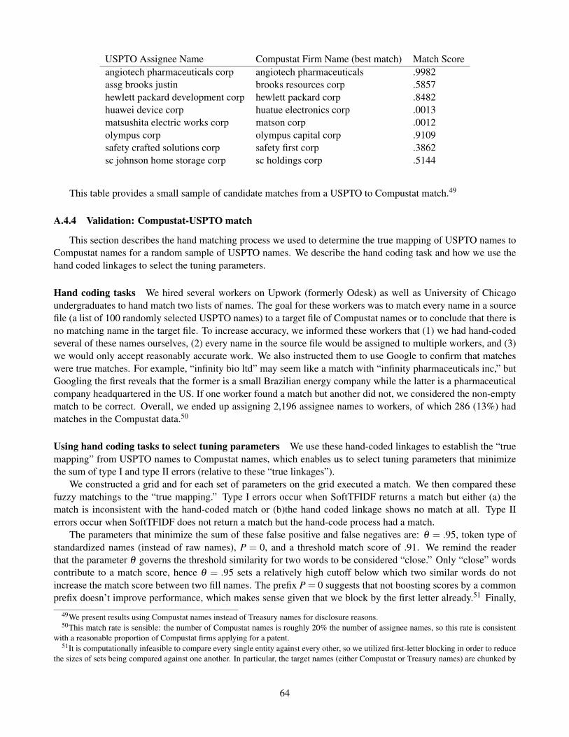
USPTO Assignee Name Compustat Firm Name (best match) Match Scoreangiotech pharmaceuticals corp angiotech pharmaceuticals .9982assg brooks justin brooks resources corp .5857hewlett packard development corp hewlett packard corp .8482huawei device corp huatue electronics corp .0013matsushita electric works corp matson corp .0012olympus corp olympus capital corp .9109safety crafted solutions corp safety first corp .3862sc johnson home storage corp sc holdings corp .5144

This table provides a small sample of candidate matches from a USPTO to Compustat match.49

A.4.4 Validation: Compustat-USPTO match

This section describes the hand matching process we used to determine the true mapping of USPTO names toCompustat names for a random sample of USPTO names. We describe the hand coding task and how we use thehand coded linkages to select the tuning parameters.

Hand coding tasks We hired several workers on Upwork (formerly Odesk) as well as University of Chicagoundergraduates to hand match two lists of names. The goal for these workers was to match every name in a sourcefile (a list of 100 randomly selected USPTO names) to a target file of Compustat names or to conclude that there isno matching name in the target file. To increase accuracy, we informed these workers that (1) we had hand-codedseveral of these names ourselves, (2) every name in the source file would be assigned to multiple workers, and (3)we would only accept reasonably accurate work. We also instructed them to use Google to confirm that matcheswere true matches. For example, “infinity bio ltd” may seem like a match with “infinity pharmaceuticals inc,” butGoogling the first reveals that the former is a small Brazilian energy company while the latter is a pharmaceuticalcompany headquartered in the US. If one worker found a match but another did not, we considered the non-emptymatch to be correct. Overall, we ended up assigning 2,196 assignee names to workers, of which 286 (13%) hadmatches in the Compustat data.50

Using hand coding tasks to select tuning parameters We use these hand-coded linkages to establish the “truemapping” from USPTO names to Compustat names, which enables us to select tuning parameters that minimizethe sum of type I and type II errors (relative to these “true linkages”).

We constructed a grid and for each set of parameters on the grid executed a match. We then compared thesefuzzy matchings to the “true mapping.” Type I errors occur when SoftTFIDF returns a match but either (a) thematch is inconsistent with the hand-coded match or (b)the hand coded linkage shows no match at all. Type IIerrors occur when SoftTFIDF does not return a match but the hand-code process had a match.

The parameters that minimize the sum of these false positive and false negatives are: θ = .95, token type ofstandardized names (instead of raw names), P = 0, and a threshold match score of .91. We remind the readerthat the parameter θ governs the threshold similarity for two words to be considered “close.” Only “close” wordscontribute to a match score, hence θ = .95 sets a relatively high cutoff below which two similar words do notincrease the match score between two fill names. The prefix P = 0 suggests that not boosting scores by a commonprefix doesn’t improve performance, which makes sense given that we block by the first letter already.51 Finally,

49We present results using Compustat names instead of Treasury names for disclosure reasons.50This match rate is sensible: the number of Compustat names is roughly 20% the number of assignee names, so this rate is consistent

with a reasonable proportion of Compustat firms applying for a patent.51It is computationally infeasible to compare every single entity against every other, so we utilized first-letter blocking in order to reduce

the sizes of sets being compared against one another. In particular, the target names (either Compustat or Treasury names) are chunked by

64

the threshold match score of .91 shows that we should only consider names a match if they are very close by oursimilarity metric. With these parameters, Type I and II errors are each below six percent.

A.4.5 Validation: Individual-inventor match

The Bell et al. (2016) inventor-level merge between patent applications and W2 reports in theory can — via theEINs provided on W2 reports — provide a linkage between patent applications and firms, but ex-ante we expectthis inventor-based match to measure something conceptually different from a firm-based match. For example,many inventors work at firms that are not the assignee of their patents, in which case we would not expect ourassignee-based merge to match to the same EIN as the Bell et al. (2016) inventor-based merge. However, theBell et al. (2016) merge nonetheless provides a very valuable benchmark for assessing the quality of our assignee-based merge. Bell et al. generously agreed to share their inventor-based merge with us, and our preliminaryresults comparing the two linkages provide a second set of evidence supporting the quality of our assignee-basedlinkage. In the simplest comparison, around 70% of patent applications are associated with the same EIN in thetwo linkages. The characteristics of this match also look sensible, e.g., the match rates are higher if we limit thesample to patent applications that Bell et al. (2016) match to inventors who all work at the same firm. Given thatwe do not expect a match rate of 100% for the reasons detailed above, we view the results of this second validationexercise as quite promising.

the first letter of their standardized names and grouped with the source (USPTO) names with the same first letter. Hence, we will miss anymatches that differ on the first letter.

65

B Appendix: Poisson model of patent value

Recall that the probability mass function for a Poisson distributed outcome Y with mean λ can be written:

p(Y |λ ) = exp(Y λ − exp(λ ))/Y !

Let Ya = (Y1, ...,Yma) and Xa = (X1, ...,Xma) denote the vectors of outcomes and covariates respectively in an

art unit a. Supposing Yj|Xaiid∼ Poisson

(X ′jδ +νa

)where νa is a scalar art unit effect, we can write:

ln p(Ya|Xa,νa) =ma

∑j=1

ln p(Yj|X ′jδ +νa

)=

ma

∑j=1

Yj(X ′jδ +νa

)− exp

(X ′jδ +νa

)− ln(Yj!)

The random effects Poisson likelihood of an art unit a can be written:

L(Ya|Xa) =1√

2πση

∫exp{

ln p(Ya|Xa)−12

ν2

σ2ν

}dν

By independence across art units, the full log likelihood can be written ∑a lnL(Ya|Xa).The first order condition for the coefficient vector δ is:

ddδ

∑a

lnL(Ya|Xa) = ∑a

∫ (∑

maj=1

[Yj− exp

(X ′jδ +ν

)]X j

)exp{

ln p(Ya|Xa,ν)− 12

ν2

σ2ν

}dν∫

exp{

ln p(Ya|Xa,ν)− 12

ν2

σ2ν

}dν

= ∑a

ma

∑j=1

[Yj−

∫exp(X ′jδ +ν

)ωa (ν)dν

]X j = 0

where the weighting function ωa (z) =exp{

ln p(Ya|Xa,z)− 12

z2

σ2ν

}∫

exp{

ln p(Ya|Xa,ν)− 12

ν2

σ2ν

}dν

is the posterior density of ν given the observables

in art unit a. Note that this is a shrunken version of the usual Poisson orthogonality condition that is robust tomisspecification of features of the conditional distribution other than the mean (Wooldridge 2010). The weights,however, rely on the exponential nature of the Poisson density function which, if misspecified, will yield inconsis-tency in small art units. In large art units, however, the posterior will spike around the “fixed effect” estimate of ν ,which is again robust to misspecification of higher moments of the conditional distribution.

The first order condition for the variance σν is:

∑a

ddσν

lnL(Ya|Xa) = ∑a

− 1ση

+

∫η2

σ3η

exp{

ln p(Ya|Xa,ν)− 12

ν2

σ2ν

}dν∫

exp{

ln p(Ya|Xa,ν)− 12

ν2

σ2ν

}dν

=

1σ3

η

∑a

[∫ωa (ν)ν

2dν−σ2ν

]= 0.

This simply says that the posterior variance of ν in each art unit should average across art units to σ2ν .

66

C Appendix: Additional figures and tables

Figure C.1: Years Until Initial Decision

0.1

.2.3

.4P

ropo

rtio

n

0 1 2 3 4 5+Decision year minus application year

Notes: This figure plots a histogram of the years until the initial patent application decision for the sample of patentassignees by application pairs in the bottom row of Panel A of Table 1 (N=99,871).

Figure C.2: Years Until Patent Grant for Initially Rejected Patent Applications

0.1

.2.3

.4.5

Pro

port

ion

Zero

One Two

Three

Four

Five Six

Seven

Eight

NineTen

+

Never

/cens

ored

Notes: This figure plots a histogram of the years until a patent grant for the subsample of patent assignee byapplication pairs in the bottom row of Panel A of Table 1 (N=99,871) which receive an initial rejection (N=88,298).

67

Figure C.3: Industry Composition of Firms

0.20.20.20.30.60.60.9

0.60.80.60.50.8

0.50.91.21.3

0.61.4

1.81.5

3.12.2

1.53.2

4.14.5

5.45.3

4.66.6

17.716.7

25.223.3

31.230.1

0 10 20 30Industry Share of Firms (% of Sample Total)

UtilitiesEducational Services

MiningArts, Entertainment, and Recreation

Management of Companies and EnterprisesAgriculture, Forestry, Fishing and Hunting

Transportation and WarehousingHealth Care and Social Assistance

Finance and InsuranceReal Estate Rental and Leasing

Accommodation and Food ServicesInformation

ConstructionOther

Retail TradeWholesale Trade

Professional Scientific and Technical ServicesManufacturing

Full Sample Initially Allowed

Notes: This figure plots the distribution of firms in our sample by industry. “Winners” are firms whose patentapplication is initially granted.

68

Tabl

eC

.1:T

estin

gfo

rSpa

tialC

orre

latio

nin

Initi

alA

llow

ance

Dec

isio

ns

Initi

ally

allo

wed

Stat

eZ

ip4-

DN

AIC

S4-

DN

AIC

S×

Stat

e(1

a)(1

b)(2

a)(2

b)(3

a)(3

b)(4

a)(4

b)

Pane

lA:a

naly

siss

ampl

e

Intr

a-cl

ass

corr

elat

ion(ρ

)0.

000

0.00

00.

068

0.05

80.

000

0.00

00.

000

0.00

0p-

valu

e1.

000

1.00

00.

297

0.46

51.

000

1.00

01.

000

1.00

0

Obs

erva

tions

9,73

28,

647

9,73

28,

647

9,73

28,

647

9,73

28,

647

Num

bero

fcat

egor

ies

5151

4,50

14,

231

355

347

3,37

63,

185

AU

-AY

FEs

Pane

lB:t

opqu

intil

e

Intr

a-cl

ass

corr

elat

ion(ρ

)0.

113

0.13

20.

000

0.00

00.

000

0.00

00.

000

0.04

6p-

valu

e0.

165

0.18

41.

000

1.00

01.

000

1.00

01.

000

0.41

6

Obs

erva

tions

1,94

61,

666

1,94

61,

666

1,94

61,

666

1,94

61,

666

Num

bero

fcat

egor

ies

4949

1,25

21,

113

250

242

1,11

91,

013

AU

-AY

FEs

Not

es:

Thi

sta

ble

repo

rts

the

resu

ltsof

test

sfo

rw

heth

erin

itial

pate

ntal

low

ance

sar

ege

ogra

phic

ally

clus

tere

d,se

para

tely

for

the

anal

ysis

sam

ple

and

fort

heto

p-qu

intil

epr

edic

ted

pate

ntva

lue

sam

ple.

“Int

ra-c

lass

corr

elat

ion(ρ

)”re

port

sth

era

tioof

ara

ndom

effe

cts

estim

ate

ofth

ege

ogra

phic

vari

ance

com

pone

ntto

the

sum

ofth

ege

ogra

phic

and

idio

sync

ratic

vari

ance

com

pone

nts.

The

p-va

lue

repo

rts

aB

reus

ch-P

agan

Lag

rang

em

ultip

lier

test

ofth

enu

llhy

poth

esis

that

ρ=0

.AU

-AY

FEs

deno

tes

the

incl

usio

nof

Art

Uni

t(A

U)b

yap

plic

atio

nye

ar(A

Y)fi

xed

effe

cts.

69

Table C.2: Mean ξ̂ by Technology Center

Technology center ξ̂ N Technology center ξ̂ N

Business Methods - Finance 15.079 152 Telecomms: Analog Radio 3.080 43Electronic Commerce 10.237 365 Mining, Roads, & Petroleum 2.991 518Databases & File Mgmt 9.726 261 Microbiology 2.983 83Tires, Adhesives, Glass, & Plastics 8.035 134 Semiconductors, Circuits, & Optics 2.903 2372180: Computer Architecture 8.029 68 Molec Bio & Bioinformatics 2.891 68Combust & Fluid Power Systems 7.803 111 Amusement & Education Devices 2.780 236Aero, Agriculture, & Weaponry 7.129 224 Static Structures & Furniture 2.627 560Selective Visual Display Systems 6.387 200 Fuel Cells & Batteries 2.437 177Computer Graphic Processing 6.012 299 Business Methods 2.416 193Optics 5.650 341 2110: Computer Architecture 2.163 50Organic Chemistry & Polymers 5.622 116 Software Development 2.141 76Organic Compounds 5.316 115 Medical Instruments 2.110 132Organic Chemistry 4.913 62 Multiplex & VoIP 1.990 72Manufact Devices & Processes 4.870 443 Metallurgy & Inorganic Chemistry 1.980 102Memory Access & Control 4.865 49 Chemical Apparatus 1.947 171Selective Communication 4.674 294 Semiconductors & Memory 1.936 185Surface Transportation 4.428 294 Cryptography & Security 1.898 76Electrical Circuits & Systems 4.090 266 Medical & Surgical Instruments 1.823 118Coating, Etching, & Cleaning 3.615 83 Computer Networks 1.733 145Misc. Computer Applications 3.459 129 Radio, Robotics, & Nucl Systems 1.597 85Material & Article Handling 3.248 255 Receptacles, Shoes, & Apparel 1.444 470Graphical User Interface 3.217 152 Kinestherapy & Exercising 1.330 138Refrigeration & Combustion 3.084 265 Fluid Handling 0.706 188

Notes: This table reports the mean predictions of ex-ante value ξ̂ by USPTO technology center of the application;technology centers are administrative groupings of art units designated by the USPTO. The sample is observationsfrom our analysis sample whose application belongs to a technology center with more than 20 observations in theanalysis sample (N=6,402). ξ̂ is measured in millions of 1982 USD.

70

Tabl

eC

.3:H

eter

ogen

eity

acro

ssla

rger

and

smal

lerfi

rms

(1)

(2)

(3)

(4)

(5)

(6)

(7)

(8)

(9)

(10)

Posi

tive

empl

oy-

men

tlo

g(Fi

rmsi

ze)

Rev

enue

per

wor

ker

Val

uead

ded

per

wor

ker

EB

ITD

per

wor

ker

Wag

ebi

llpe

rw

orke

r

Surp

lus

per

wor

ker

Lab

orco

mp

per

wor

ker

W2

+10

99pe

rw

orke

r

Ave

rage

stay

erea

rnin

gs

Pane

lA:l

arge

firm

s

Hig

hva

lue

(Q5)

0.05

0.20

39.3

614

.04

8.89

2.16

10.6

71.

691.

986.

81(0

.03)

(0.0

7)(1

7.51

)(6

.95)

(5.3

8)(2

.73)

(6.2

6)(3

.74)

(2.1

0)(3

.13)

Mea

nof

outc

ome

(Q5)

0.74

3.87

263.

7096

.66

7.87

53.4

261

.94

46.8

248

.20

67.8

0%

Impa

ct(Q

5)7.

35.

214

.914

.511

2.9

4.0

17.2

3.6

4.1

10.0

Low

erva

lue

(<Q

5)0.

01-0

.07

1.71

4.78

-0.0

3-0

.18

0.25

2.10

-0.4

6-1

.48

(0.0

2)(0

.05)

(11.

48)

(5.1

3)(2

.64)

(1.1

5)(3

.08)

(1.7

9)(1

.32)

(2.3

2)

Pane

lB:s

mal

lfirm

s

Hig

hva

lue

(Q5)

-0.1

00.

2819

.59

16.5

68.

825.

1513

.28

7.37

2.99

7.52

(0.0

8)(0

.15)

(25.

06)

(7.6

8)(4

.03)

(3.0

8)(5

.18)

(4.4

1)(3

.69)

(6.6

8)M

ean

ofou

tcom

e(Q

5)0.

651.

6431

2.10

127.

2010

.47

51.3

963

.64

56.4

342

.35

64.5

5%

Impa

ct(Q

5)-1

5.8

16.8

6.3

13.0

84.2

10.0

20.9

13.1

7.1

11.7

Low

erva

lue

(<Q

5)-0

.02

0.13

-22.

21-3

.57

-2.9

31.

81-0

.89

0.49

1.48

6.88

(0.0

2)(0

.06)

(14.

07)

(5.5

7)(1

.95)

(1.2

6)(2

.36)

(2.3

5)(0

.98)

(2.2

3)

Obs

erva

tions

155,

646

103,

437

103,

437

103,

437

103,

437

103,

437

103,

437

103,

437

107,

789

99,5

58

Not

es:

Thi

sta

ble

repo

rts

diff

eren

ce-i

n-di

ffer

ence

ses

timat

esof

the

effe

ctof

initi

alpa

tent

allo

wan

ces

inte

ract

edw

ithla

rge

and

smal

lfirm

size

onfir

man

dw

orke

rout

com

es,s

epar

atel

yfo

rhig

han

dlo

wex

-ant

eva

luab

lepa

tent

appl

icat

ions

,in

oura

naly

sis

sam

ple.

Lar

gefir

ms

are

thos

eab

ove

med

ian

base

line

empl

oym

ent,

and

smal

lfirm

sar

eth

ose

belo

wm

edia

nba

selin

eem

ploy

men

t.E

stim

ates

corr

espo

ndto

coef

ficie

nts

onin

tera

ctio

nsof

the

desi

gnat

edva

lue

cate

gory

with

apo

st-d

ecis

ion

indi

cato

r,an

indi

cato

rfo

rth

eap

plic

atio

nbe

ing

initi

ally

allo

wed

,and

whe

ther

the

empl

oym

ento

fth

efir

mw

asab

ove

orbe

low

med

ian

base

line

empl

oym

ent.

Con

trol

sin

clud

em

ain

effe

ctof

valu

eca

tego

ryin

tera

cted

with

apo

st-d

ecis

ion

indi

cato

r,fir

mfix

edef

fect

s,an

dar

tun

itby

appl

icat

ion

year

byca

lend

arye

arfix

edef

fect

s.St

anda

rder

rors

(rep

orte

din

pare

nthe

ses)

are

two-

way

clus

tere

dby

(1)a

rtun

it,an

d(2

)app

licat

ion

year

byde

cisi

onye

ar.P

anel

Are

port

sthe

estim

ates

fort

hela

rge

firm

indi

cato

rint

erac

ted

with

apo

st-d

ecis

ion

indi

cato

rand

anin

itial

allo

wan

cein

dica

tor.

Pane

lBre

port

sth

ees

timat

esfo

rth

esm

allfi

rmin

tera

cted

with

apo

st-d

ecis

ion

indi

cato

ran

dan

initi

alal

low

ance

indi

cato

r.E

BIT

Dis

earn

ings

befo

rein

tere

st,t

axes

,and

dedu

ctio

ns.S

urpl

usis

EB

ITD

+w

age

bill.

Stay

ersa

rede

fined

asth

ose

who

wer

eem

ploy

edby

the

sam

efir

min

the

year

ofap

plic

atio

n.L

abor

com

pens

atio

nm

easu

res

tota

lded

uctio

nsfo

rla

bor

expe

nses

clai

med

byth

efir

m.

“W2

+10

99”

mea

sure

sto

the

sum

ofW

2an

d10

99ea

rnin

gsdi

vide

dby

the

sum

ofth

enu

mbe

rof

W2’

san

d10

99’s

filed

.“%

Impa

ct”

repo

rts

the

perc

entc

hang

ein

the

outc

ome

atth

em

ean

for

win

ning

anin

itial

allo

wan

ce.R

even

ue,v

alue

adde

d,E

BIT

D,w

age

bill,

surp

lus,

earn

ings

,lab

orco

mpe

nsat

ion,

and

W2

+10

99pa

yar

ere

port

edin

thou

sand

sof

2014

USD

.

71

Tabl

eC

.4:W

ithin

-Fir

mIn

equa

lity

(1)

(2)

(3)

(4)

(5)

(6)

(7)

(8)

(9)

Avg

mal

eea

rnin

gs

Avg

fem

ale

earn

ings

Gen

der

earn

ings

gap

Avg

inve

ntor

earn

ings

Avg

earn

ings

ofno

n-in

vent

ors

Inve

ntor

earn

ings

gap

Wag

ebi

llpe

rw

orke

r(Q

1)

Wag

ebi

llpe

rw

orke

r(Q

4)

Wag

ebi

llpe

rwor

ker

(Q4−

Q1)

Hig

hva

lue

(Q5)

5.88

0.15

6.90

16.8

72.

2414

.92

-0.0

48.

068.

12(1

.97)

(1.5

1)(1

.97)

(8.4

7)(1

.43)

(7.7

5)(1

.01)

(2.8

5)(2

.56)

Mea

nof

outc

ome

(Q5)

60.9

736

.69

24.4

213

0.20

47.6

481

.49

16.6

111

0.70

94.1

7%

Impa

ct(Q

5)9.

70.

428

.313

.04.

718

.3-0

.37.

38.

6

Low

erva

lue

(<Q

5)0.

35-0

.49

-0.0

6-1

.24

0.47

-1.7

20.

052.

822.

77(1

.16)

(0.5

1)(1

.06)

(4.6

0)(0

.81)

(4.7

0)(0

.32)

(2.4

2)(2

.34)

Obs

erva

tions

95,0

0484

,562

80,2

2252

,471

100,

901

50,0

4582

,750

81,5

3681

,536

Not

es:

Thi

sta

ble

repo

rts

diff

eren

ce-i

n-di

ffer

ence

ses

timat

esof

the

effe

ctof

initi

alpa

tent

allo

wan

ces

onw

ithin

-firm

ineq

ualit

ym

easu

res,

sepa

rate

lyfo

rhi

ghan

dlo

wex

-ant

eva

luab

lepa

tent

appl

icat

ions

,in

our

anal

ysis

sam

ple.

Est

imat

esco

rres

pond

toco

effic

ient

son

inte

ract

ions

ofth

ede

sign

ated

valu

eca

tego

ryw

itha

post

-dec

isio

nin

dica

tora

ndan

indi

cato

rfor

the

appl

icat

ion

bein

gin

itial

lyal

low

ed.C

ontr

ols

incl

ude

mai

nef

fect

ofva

lue

cate

gory

inte

ract

edw

itha

post

-dec

isio

nin

dica

tor,

firm

fixed

effe

cts,

and

artu

nitb

yap

plic

atio

nye

arby

cale

ndar

year

fixed

effe

cts,

asin

equa

tion

(8).

Stan

dard

erro

rs(r

epor

ted

inpa

rent

hese

s)ar

etw

o-w

aycl

uste

red

by(1

)ar

tuni

t,an

d(2

)ap

plic

atio

nye

arby

deci

sion

year

.“G

ende

rea

rnin

gsga

p”m

easu

res

the

diff

eren

cebe

twee

nav

erag

em

ale

and

fem

ale

earn

ings

atfir

ms

whe

rebo

thge

nder

sar

epr

esen

t.“I

nven

tore

arni

ngs

gap”

mea

sure

sth

edi

ffer

ence

betw

een

aver

age

inve

ntor

and

non-

inve

ntor

earn

ings

atfir

ms

whe

rebo

thin

vent

ors

and

non-

inve

ntor

sar

epr

esen

t.“W

age

bill

per

wor

ker(Q

1)”

mea

sure

sth

eav

erag

ew

age

bill

inw

ithin

-firm

wag

equ

artil

eon

e.“W

age

bill

per

wor

ker(Q

4)”

mea

sure

sth

eav

erag

ew

age

bill

inw

ithin

-firm

wag

equ

artil

efo

ur.

“Wag

ebi

llpe

rw

orke

r(Q

4−

Q1)

”m

easu

res

the

diff

eren

cebe

twee

nav

erag

eQ

4an

dQ

1ea

rnin

gs.

Stay

ers

are

defin

edas

thos

ew

how

ere

empl

oyed

byth

esa

me

firm

inth

eye

arof

appl

icat

ion.

Ent

rant

sar

ede

fined

asth

ose

empl

oyee

sw

how

ere

note

mpl

oyed

atth

efir

min

the

prev

ious

year

.Ear

ning

san

dw

age

bill

are

mea

sure

din

thou

sand

sof

2014

USD

.

72

Tabl

eC

.5:W

ithin

-Fir

mIn

equa

lity

(Usi

nga

Bal

ance

dSa

mpl

e)

(1)

(2)

(3)

(4)

(5)

(6)

(7)

(8)

(9)

Avg

mal

eea

rnin

gs

Avg

fem

ale

earn

ings

Gen

der

earn

ings

gap

Avg

inve

ntor

earn

ings

Avg

earn

ings

ofno

n-in

vent

ors

Inve

ntor

earn

ings

gap

Wag

ebi

llpe

rw

orke

r(Q

1)

Wag

ebi

llpe

rw

orke

r(Q

4)

Wag

ebi

llpe

rw

orke

r(Q

4−

Q1)

Hig

hva

lue

(Q5)

7.11

0.21

6.90

14.4

4-0

.48

14.9

2-0

.06

8.06

8.12

(1.7

9)(1

.54)

(1.9

7)(7

.59)

(1.8

6)(7

.75)

(1.0

1)(2

.85)

(2.5

6)M

ean

ofou

tcom

e(Q

5)61

.45

37.0

324

.42

132.

3050

.76

81.4

916

.55

110.

7094

.17

%Im

pact

(Q5)

11.6

0.6

28.3

10.9

-1.0

18.3

-0.3

7.3

8.6

Low

erva

lue

(<Q

5)-0

.23

-0.1

8-0

.06

-1.3

50.

37-1

.72

0.05

2.82

2.77

(1.1

2)(0

.45)

(1.0

6)(4

.91)

(1.1

8)(4

.70)

(0.3

2)(2

.42)

(2.3

4)

Obs

erva

tions

80,2

2280

,222

80,2

2250

,045

50,0

4550

,045

81,5

3681

,536

81,5

36

Not

es:

Thi

stab

lere

plic

ates

Tabl

eC

.4us

ing

aco

mm

onsa

mpl

efo

reac

hco

mpa

riso

ngr

oup.

Eac

hco

lum

nre

port

sdiff

eren

ce-i

n-di

ffer

ence

sest

imat

esof

the

effe

ctof

initi

alpa

tent

allo

wan

ces

onw

ithin

-firm

ineq

ualit

ym

easu

res,

sepa

rate

lyfo

rhi

ghan

dlo

wex

-ant

eva

luab

lepa

tent

appl

icat

ions

,in

asu

bsam

ple

ofou

ran

alys

issa

mpl

ew

here

the

com

posi

tion

offir

ms

ishe

ldco

nsta

ntac

ross

the

rela

ted

outc

ome

colu

mns

.E

stim

ates

corr

espo

ndto

coef

ficie

nts

onin

tera

ctio

nsof

the

desi

gnat

edva

lue

cate

gory

with

apo

st-d

ecis

ion

indi

cato

ran

dan

indi

cato

rfo

rth

eap

plic

atio

nbe

ing

initi

ally

allo

wed

.C

ontr

ols

incl

ude

mai

nef

fect

ofva

lue

cate

gory

inte

ract

edw

itha

post

-dec

isio

nin

dica

tor,

firm

fixed

effe

cts,

and

artu

nitb

yap

plic

atio

nye

arby

cale

ndar

year

fixed

effe

cts.

Stan

dard

erro

rs(r

epor

ted

inpa

rent

hese

s)ar

etw

o-w

aycl

uste

red

by(1

)ar

tun

it,an

d(2

)ap

plic

atio

nye

arby

deci

sion

year

.“G

ende

rea

rnin

gsga

p”m

easu

res

the

diff

eren

cebe

twee

nav

erag

em

ale

and

fem

ale

earn

ings

atfir

ms

whe

rebo

thge

nder

sar

epr

esen

t.“I

nven

tor

earn

ings

gap”

mea

sure

sth

edi

ffer

ence

betw

een

aver

age

inve

ntor

and

non-

inve

ntor

earn

ings

atfir

ms

whe

rebo

thin

vent

ors

and

non-

inve

ntor

sar

epr

esen

t.“W

age

bill

per

wor

ker

(Q1)

”m

easu

res

the

aver

age

wag

ebi

llin

with

in-fi

rmw

age

quar

tile

one.

“Wag

ebi

llpe

rwor

ker(

Q4)

”m

easu

res

the

aver

age

wag

ebi

llin

with

in-fi

rmw

age

quar

tile

four

.“W

age

bill

perw

orke

r(Q

4−

Q1)

”m

easu

res

the

diff

eren

cebe

twee

nav

erag

eQ

4an

dQ

1ea

rnin

gs.“

%Im

pact

”re

port

sth

epe

rcen

tcha

nge

inth

eou

tcom

eat

the

mea

nfo

rwin

ning

anin

itial

allo

wan

ce.E

arni

ngs

and

wag

ebi

llar

em

easu

red

inth

ousa

nds

of20

14U

SD.

73

Tabl

eC

.6:E

arni

ngs

Impa

cts

bySt

ayer

Subg

roup

s

(1)

(2)

(3)

(4)

(5)

(6)

Avg

mal

est

ayer

earn

ings

Avg

fem

ale

stay

erea

rnin

gsSt

ayer

gend

erea

rnin

gsga

pA

vgin

vent

orst

ayer

earn

ings

Avg

non-

inve

ntor

stay

erea

rnin

gsSt

ayer

inve

ntor

earn

ings

gap

Hig

hva

lue

(Q5)

13.8

32.

738.

8917

.41

5.75

9.27

(2.7

4)(1

.95)

(3.5

1)(1

1.21

)(1

.72)

(8.3

5)M

ean

ofou

tcom

e(Q

5)85

.03

48.3

537

.77

156.

0064

.37

91.8

5%

Impa

ct(Q

5)16

.35.

723

.511

.28.

910

.1

Low

erva

lue

(<Q

5)2.

170.

70-0

.83

0.58

2.03

-2.7

8(1

.96)

(0.8

3)(1

.80)

(6.3

1)(1

.26)

(6.9

1)

Obs

erva

tions

88,1

0071

,591

66,2

7047

,063

94,9

0942

,640

Not

es:

Thi

sta

ble

repo

rts

diff

eren

ce-i

n-di

ffer

ence

ses

timat

esof

the

effe

ctof

initi

alpa

tent

allo

wan

ces

onw

ithin

-firm

ineq

ualit

ym

easu

res,

sepa

rate

lyfo

rhi

ghan

dlo

wex

-ant

eva

luab

lepa

tent

appl

icat

ions

,in

asu

bsam

ple

ofou

ran

alys

issa

mpl

ew

here

the

com

posi

tion

offir

ms

ishe

ldco

nsta

ntac

ross

the

rela

ted

outc

ome

colu

mns

.E

stim

ates

corr

espo

ndto

coef

ficie

nts

onin

tera

ctio

nsof

the

desi

gnat

edva

lue

cate

gory

with

apo

st-d

ecis

ion

indi

cato

ran

dan

indi

cato

rfo

rth

eap

plic

atio

nbe

ing

initi

ally

allo

wed

.C

ontr

ols

incl

ude

mai

nef

fect

ofva

lue

cate

gory

inte

ract

edw

itha

post

-dec

isio

nin

dica

tor,

firm

fixed

effe

cts,

and

artu

nitb

yap

plic

atio

nye

arby

cale

ndar

year

fixed

effe

cts.

Stan

dard

erro

rs(r

epor

ted

inpa

rent

hese

s)ar

etw

o-w

aycl

uste

red

by(1

)ar

tuni

t,an

d(2

)app

licat

ion

year

byde

cisi

onye

ar.“

Stay

erge

nder

earn

ings

gap”

mea

sure

sth

edi

ffer

ence

betw

een

aver

age

mal

est

ayer

and

fem

ale

stay

erea

rnin

gsat

firm

sw

here

both

gend

ers

are

pres

ent.

“Sta

yeri

nven

tore

arni

ngs

gap”

mea

sure

sth

edi

ffer

ence

betw

een

aver

age

inve

ntor

stay

eran

dno

n-in

vent

orst

ayer

earn

ings

atfir

ms

whe

rebo

thin

vent

ors

and

non-

inve

ntor

sar

epr

esen

t.“%

Impa

ct”

repo

rts

the

perc

entc

hang

ein

the

outc

ome

atth

em

ean

forw

inni

ngan

initi

alal

low

ance

.St

ayer

sar

ede

fined

asth

ose

who

wer

eem

ploy

edby

the

sam

efir

min

the

year

ofap

plic

atio

n.E

arni

ngs

are

mea

sure

din

thou

sand

sof

2014

USD

.

74

Tabl

eC

.7:E

arni

ngs

ofO

ffice

rs/O

wne

rs

All

firm

sPa

ss-t

hrou

ghen

titie

s

(1)

(2)

(3)

(4)

(5)

(6)

(7)

(8)

(9)

Offi

cer

earn

ings

perW

2

Wag

esan

dsa

lari

espe

rW2

Non

-of

ficer

com

ppe

rW

2

Offi

cer

earn

ings

perW

2

Wag

esan

dsa

lari

espe

rW

2N

on-o

ffice

rco

mp

perW

2

Avg

earn

ings

ofow

ner-

empl

oyee

s

Avg

pay

ofow

ner-

empl

oyee

s

Avg

W2

earn

ings

ofno

n-ow

ner-

empl

oyee

s

Hig

hva

lue

(Q5)

3.81

0.13

-0.0

57.

17-1

.43

-1.6

742

.87

84.0

85.

99(1

.31)

(1.8

9)(2

.10)

(3.2

7)(1

.66)

(1.5

6)(1

7.01

)(4

1.36

)(2

.41)

Mea

nof

outc

ome

(Q5)

15.8

935

.07

38.9

114

.86

27.8

531

.25

149.

7024

6.60

41.7

6%

Impa

ct(Q

5)24

.00.

4-0

.148

.3-5

.1-5

.428

.634

.114

.4

Low

erva

lue

(<Q

5)-0

.83

1.46

1.97

-1.2

80.

461.

22-0

.28

-3.7

10.

66(0

.94)

(1.0

1)(1

.02)

(1.3

8)(1

.31)

(1.4

9)(5

.45)

(18.

72)

(0.8

4)

Obs

erva

tions

103,

437

103,

437

103,

437

49,9

4349

,943

49,9

4331

,962

45,3

1843

,531

Not

es:

Thi

sta

ble

repo

rts

diff

eren

ce-i

n-di

ffer

ence

ses

timat

esof

the

effe

ctof

initi

alpa

tent

allo

wan

ces

onof

ficer

and

non-

offic

erea

rnin

gsm

easu

res

for

allfi

rms

and

pass

-thr

ough

entit

ies.

Est

imat

esco

rres

pond

toco

effic

ient

son

inte

ract

ions

ofth

ede

sign

ated

valu

eca

tego

ryw

itha

post

-dec

isio

nin

dica

tor

and

anin

dica

torf

orth

eap

plic

atio

nin

itial

lyal

low

ed.C

ontr

ols

incl

ude

mai

nef

fect

ofva

lue

cate

gory

inte

ract

edw

itha

post

-dec

isio

nin

dica

tor,

firm

fixed

effe

cts,

and

artu

nitb

yap

plic

atio

nye

arby

cale

ndar

year

fixed

effe

cts.

Stan

dard

erro

rs(r

epor

ted

inpa

rent

hese

s)ar

etw

o-w

aycl

uste

red

by(1

)art

unit,

and

(2)a

pplic

atio

nye

arby

deci

sion

year

.“%

Impa

ct”

repo

rts

the

perc

entc

hang

ein

the

outc

ome

atth

em

ean

forw

inni

ngan

initi

alal

low

ance

.E

arni

ngs

are

mea

sure

din

thou

sand

sof

2014

USD

.The

outc

ome

vari

able

sar

ede

fined

asfo

llow

s.(1

)Offi

cere

arni

ngs

perW

2is

the

offic

erco

mpe

nsat

ion

com

pone

ntof

labo

rco

mpe

nsat

ion

that

we

defin

ein

A.3

.Sp

ecifi

cally

,the

num

erat

orof

(1)

isL

ine

12on

C-c

orpo

ratio

nfo

rm11

20,l

ine

7on

S-co

rpor

atio

nfo

rm11

20S,

and

line

10on

Part

ners

hip

form

1065

.E

ach

ofth

ese

line

num

bers

corr

espo

nds

toth

e20

10IR

Sfo

rms.

Sim

ilarl

y,th

enu

mer

ator

ofC

olum

n(2

)is

the

sala

ries

and

wag

esco

mpo

nent

ofla

bor

com

pens

atio

n,w

hich

islin

e13

,8,a

nd9

onth

eC

-cor

pora

tion,

S-co

rpor

atio

n,an

dpa

rtne

rshi

pfo

rms,

resp

ectiv

ely.

The

num

erat

orof

colu

mn

(3)

isla

bor

com

pens

atio

nle

ssof

ficer

com

pens

atio

n,so

itin

clud

esth

eot

her

com

pone

nts

ofla

bor

com

pens

atio

n(i

.e.,

itin

clud

essa

lari

esan

dw

ages

,pen

sion

profi

t-sh

arin

gpl

ans,

and

empl

oyee

bene

fitpr

ogra

ms)

.O

nfo

rm11

20,f

orex

ampl

e,th

ese

are

lines

13,2

3,an

d24

.C

olum

ns(4

)-(6

)re

stri

ctth

esa

mpl

eto

only

S-co

rpor

atio

nsan

dPa

rtne

rshi

ps,b

utha

veth

esa

me

defin

ition

s,re

spec

tivel

y,as

Col

umns

(1)-

(3).

Col

umn

(7)

isth

eav

erag

eW

2w

age

earn

ings

that

goto

firm

owne

rs,w

hich

was

cons

truc

ted

usin

gm

atch

edfir

m-o

wne

rda

tafr

omSm

ithet

al.(

2017

).Sp

ecifi

cally

,for

each

S-co

rpor

atio

nan

dpa

rtne

rshi

p,w

eca

lcul

ate

the

sum

ofW

2w

ages

that

accr

ueto

itsow

ners

and

divi

deth

issu

mby

the

num

ber

ofow

ners

who

also

getp

ositi

veW

2in

com

efr

omth

efir

m.C

olum

n(8

)is

aver

age

owne

rpay

,whi

chis

the

sum

ofW

2w

age

earn

ings

that

accr

ueto

owne

rspl

usth

eirb

usin

ess

inco

me

divi

ded

byth

enu

mbe

rofo

wne

rs.E

ach

owne

rs’b

usin

ess

inco

me

com

esfr

omSm

ithet

al.(

2017

)’s

linka

gebe

twee

nfir

ms

and

owne

rs,w

hich

was

cons

truc

ted

usin

gSc

hedu

leK

1of

form

1120

Sfo

rS-

corp

orat

ions

and

form

1065

for

Part

ners

hips

.B

eing

able

toid

entif

ybu

sine

ssow

ners

dire

ctly

ison

lypo

ssib

lefo

rS-

corp

orat

ions

and

part

ners

hips

,so

only

aggr

egat

efir

m-l

evel

busi

ness

inco

me

isav

aila

ble

for

C-c

orpo

ratio

ns(o

nlin

e28

offo

rm11

20).

Fina

lly,C

olum

n(9

)is

the

tota

lW2

earn

ings

forn

on-o

wne

rsdi

vide

dby

the

num

bero

fnon

-ow

nerW

2s.

75

Tabl

eC

.8:P

ass-

Thr

ough

Est

imat

es:T

hree

-Yea

rAve

rage

ofSu

rplu

spe

rWor

ker

Wag

ebi

llpe

rw

orke

rA

vgm

ale

earn

ings

Avg

non-

inve

ntor

earn

ings

Avg

stay

erea

rnin

gs

Avg

earn

ings

ofst

ayer

sm

inus

earn

ings

inap

pyr

Avg

non-

inve

ntor

stay

erea

rnin

gs

(1a)

(1b)

(2a)

(2b)

(3a)

(3b)

(4a)

(4b)

(5a)

(5b)

(6a)

(6b)

OL

SIV

OL

SIV

OL

SIV

OL

SIV

OL

SIV

OL

SIV

Surp

lus

/wor

ker

0.20

0.35

0.23

0.70

0.16

0.31

0.26

0.66

0.25

0.61

0.21

0.60

(0.0

1)(0

.15)

(0.0

1)(0

.25)

(0.0

1)(0

.14)

(0.0

1)(0

.34)

(0.0

1)(0

.32)

(0.0

1)(0

.28)

Ela

stic

ity0.

243

0.42

30.

242

0.72

90.

215

0.41

10.

253

0.64

1.

.0.

224

0.65

1

Obs

erva

tions

83,2

1283

,212

77,0

6677

,066

81,6

3281

,632

81,0

7581

,075

81,0

7581

,075

77,9

3977

,939

1st s

tage

F8.

006.

216.

388.

588.

585.

97E

xoge

neity

0.28

40.

045

0.25

70.

179

0.21

60.

072

Not

es:

Thi

stab

lere

port

sOL

San

dIV

estim

ates

ofth

eef

fect

ofin

crea

sesi

nsu

rplu

sper

wor

kero

nse

lect

edea

rnin

gsou

tcom

esus

ing

thre

e-ye

arav

erag

esof

surp

lus

perw

orke

r.T

heex

clud

edin

stru

men

tis

the

inte

ract

ion

ofto

pqu

intil

eof

ex-a

nte

valu

eξ̂

cate

gory

with

apo

st-d

ecis

ion

indi

cato

rand

anin

dica

tor

for

the

appl

icat

ion

bein

gin

itial

lyal

low

ed.

Con

trol

sin

clud

em

ain

effe

ctof

valu

eca

tego

ryin

tera

cted

with

post

-dec

isio

nin

dica

tor

and

inte

ract

ion

oflo

wer

quin

tile

valu

eca

tego

ryw

itha

post

-dec

isio

nin

dica

tor

times

anin

dica

tor

for

initi

ally

allo

wed

,firm

fixed

effe

cts,

and

artu

nitb

yap

plic

atio

nye

arby

cale

ndar

year

fixed

effe

cts.

Stan

dard

erro

rs(r

epor

ted

inpa

rent

hese

s)ar

etw

o-w

aycl

uste

red

by(1

)art

unit,

and

(2)a

pplic

atio

nye

arby

deci

sion

year

.“E

xoge

neity

”re

port

sp-

valu

efo

rtes

tofn

ullh

ypot

hesi

sth

atIV

and

OL

Ses

timat

ors

have

sam

epr

obab

ility

limit.

Stay

ers

are

defin

edas

thos

ew

how

ere

empl

oyed

byth

esa

me

firm

inth

eye

arof

appl

icat

ion.

Surp

lus

isE

BIT

D(e

arni

ngs

befo

rein

tere

st,t

ax,a

ndde

prec

iatio

n)+

wag

ebi

ll.E

arni

ngs,

wag

ebi

ll,an

dsu

rplu

sar

em

easu

red

inth

ousa

nds

of20

14U

SD.

76

Tabl

eC

.9:S

ensi

tivity

anal

ysis

ofre

tent

ion

estim

ates

and

mod

elba

sed

inte

rpre

tatio

n

(1)

(2)

(3)

(4)

(5)

(6)

Bas

elin

eL

owin

cum

bent

prem

ium

Hig

hre

tent

ion

elas

ticity

Low

rete

ntio

nel

astic

ityH

igh

pass

-th

roug

hra

teL

owpa

ss-

thro

ugh

rate

Pane

lA.C

alib

rate

dw

age

prem

ium

Cal

ibra

ted

inpu

tsw

I j/w

m j1.

81.

21.

81.

81.

81.

8

dln

G( w

I j) /dln

wI j

1.2

1.2

1.8

0.6

1.2

1.2

π0.

610.

610.

610.

610.

910.

31

Mod

el-b

ased

outp

uts

η2.

77.

34.

01.

42.

72.

7c′(N

j/I j)/

wm j

1.1

0.2

1.0

1.4

1.1

1.1

θ0.

730.

880.

800.

590.

730.

73ε

6.0

3.3

4.2

--

1.7

Pane

lB.C

alib

rate

del

astic

ityof

prod

uctd

eman

dC

alib

rate

din

puts

ε6.

06.

06.

06.

0

dln

G( w

I j) /dln

wI j

1.8

0.6

1.2

1.2

π0.

610.

610.

910.

31

Mod

el-b

ased

outp

uts

wI j/

wm j

2.9

1.3

--

η2.

72.

7-

0.6

c′(N

j/I j)/

wm j

2.6

0.4

--

θ0.

730.

73-

0.37

Not

es:

Thi

sta

ble

repo

rts

estim

ates

ofm

odel

-bas

edpa

ram

eter

sun

der

diff

eren

tca

libra

tions

ofth

ere

tent

ion

elas

ticity

and

pass

-thr

ough

rate

.Pa

nel

Aal

low

sfo

rdi

ffer

entc

alib

ratio

nsof

the

incu

mbe

ntw

age

prem

ium

wI j/

wm j

.C

olum

n(1

)re

port

sou

rba

selin

eca

libra

tion,

whe

reth

ew

age

prem

ium

isth

era

tioof

the

aver

age

earn

ings

ofin

cum

bent

wor

kers

toav

erag

eea

rnin

gsof

rece

nten

tran

tsin

the

year

ofap

plic

atio

n.T

heba

selin

ere

tent

ion

elas

ticity

dln

G( w

I j) /dln

wI j

ises

timat

edin

Tabl

eC

.1an

dth

epa

ss-t

hrou

ghra

teis

estim

ated

inTa

ble

8.C

olum

n(2

)re

calib

rate

sal

lm

odel

-bas

edpa

ram

eter

sas

sum

ing

alo

wer

wag

epr

emiu

mof

1.2.

Col

umns

(3)

and

(4)

reca

libra

teas

sum

ing

the

rete

ntio

nel

astic

ityis

one

stan

dard

devi

atio

nab

ove

and

belo

wth

eba

selin

e,re

spec

tivel

y.C

olum

ns(5

)an

d(6

)re

-est

imat

eth

em

odel

-bas

edpa

ram

eter

sas

sum

ing

the

pass

-thr

ough

rate

ison

est

anda

rdde

viat

ion

abov

ean

dbe

low

the

base

line,

resp

ectiv

ely.

Pane

lBho

lds

the

base

line

elas

ticity

ofpr

oduc

tdem

and

εco

nsta

ntan

dal

low

sth

ew

age

prem

ium

tova

ry.C

olum

n(1

)in

Pane

lBw

ould

repl

icat

eth

eba

selin

ere

sults

,so

itw

asex

clud

edfr

omth

ista

ble.

Col

umn

(2)

isno

trep

orte

din

Pane

lBas

itre

port

sth

ere

sults

ofca

libra

ting

the

incu

mbe

ntw

age

prem

ium

.D

ashe

sde

note

case

sin

whi

chth

epa

ram

eter

valu

elie

sou

tsid

ea

feas

ible

rang

e.Se

eSe

ctio

n2

for

how

the

para

met

ers

are

calc

ulat

ed.

77