who leaves and who stays? outmigration of estonian
TRANSCRIPT

Who leaves and who stays? Outmigration
of Estonian immigrants from Finland and
its impact on economic assimilation of
Estonian immigrants in Finland
Mari Kangasniemi and Merja Kauhanen
NORFACE MIGRATION Discussion Paper No. 2013-01
www.norface-migration.org

1
Who leaves and who stays? Outmigration of Estonian immigrants from Finland and itsimpact on economic assimilation of Estonian immigrants in Finland1
Mari Kangasniemi and Merja KauhanenLabour Institute for Economic ResearchPitkänsillanranta 3 A 00530 HelsinkiFinland
Abstract
This paper investigates the outmigration of Estonian immigrants from Finland and their economic
assimilation. We use a register-based panel data set on new Estonian immigrants from the years
2000 to 2006 to analyse the determinants of outmigration in a duration model framework and to
examine the economic assimilation of Estonian immigrants in terms of wages and employment. The
results show that earnings have a negative coefficient in the estimated hazard function, in particular
when interacted with the second to the fourth years of migration spells. In terms of employment,
there is a considerable employment differential between immigrants and natives in the first year of
immigration spells, but this gap narrows over time even in the longest observed durations.
Employment assimilation also occurs within individual work histories. For wages, the initial
immigrant-native gap is heavily dependent on the age at arrival and gender. Though immigrants
initially gain in terms of wage, this trend fades after a few years. When we exclude those who are
identified as outmigrants we observe qualitatively similar patterns.
Keywords: migration, temporary migration, immigrant assimilation, employment, earnings
JEL code: J15, J61
1 This study is part of the project ‘Migrant Diversity and Regional Disparity in Europe’ funded by NORFACE.(NORFACE-496, MIDIREDIE). Financial support from NORFACE research programme on Migration in Europe -Social, Economic, Cultural and Policy Dynamics is gratefully acknowledged. We also thank the participants of the 2011Summer Meeting of Finnish economists in Jyväskylä, ERSA 2011 conference, 3rd NORFACE Migration conference inMannheim and the seminar of the Labour Institute for Economic Research for useful comments. Any errors remain oursole responsibility.

2
1. Introduction
Permanent migration and its consequences have been widely researched in the economic literature.
Although temporary migration is a significant phenomenon of migration behaviour, i.e. many of the
immigrants leave the host country after some time2, the role of outmigration has been frequently
neglected in the analysis of the economic consequences of immigration. In particular, less attention
has been paid in empirical literature to the selective nature of outmigration, i.e. those migrants who
leave the host country are not randomly selected. Yet outmigration patterns may have significant
consequences for the overall contribution of immigrants to the host country (Constant and Massey,
2003). The timing of emigration and the profiles of those who leave and those who stay have an
impact on immigrants’ contribution to the tax base and welfare participation (Reagan and Olsen,
2000). If outmigrants are non-randomly selected, outmigration may also distort measures of
assimilation. It is also important to take selective emigration into account when one is measuring
the economic effect of immigration on natives: temporary migration may lead to heterogeneity in
assimilation patterns, as well as across immigrants, which cannot be captured by the standard set of
human capital variables. Understanding factors that influence outmigration are also important for
designing immigration policies.
The purpose of this paper is to study the determinants of the outmigration of Estonian immigrants in
Finland, and to study the economic assimilation of immigrants as measured by the convergence of
earnings and employment in comparison with working-age natives and also to observe the impact
of selective outmigration. We utilise a register-based panel data set of new Estonian immigrants in
Finland from the years 2000 to 2007 and we attempt to control for unobserved heterogeneity in our
analyses by using the standard panel methods. We also contribute to the earlier literature by
providing new information about re-migration and economic assimilation patterns among
immigrants in the context of East-West migration. We focus on Estonian immigrants who constitute
the second largest immigrant group in Finland and of which group a non-negligible number re-
migrate within a couple of years of their arrival. The Estonian-Finnish country-pair provides an
interesting case for analysing re-migration patterns: Finland and Estonia represent neighbouring
countries with similar languages, but the wage and welfare gaps are of significant magnitude. As
2 A large proportion of economic migrations are temporary, and immigrants are inclined to return to their countries oforigin. Return migration is the most common form of temporary migration. The other sub-categories of temporarymigration are contract, circulatory and transient migration (Dustmann et al. 2003).

3
our data covers the time before and after Estonia joined the EU, we are also able to observe the
impact of Estonia’s EU membership on Estonian immigrants’ outmigration behaviour.
Our results show that outmigration may be partly explained by poor labour market performance:
being outside the labour force has a positive coefficient in the estimated hazard of outmigration, and
higher labour-related income has a negative coefficient in certain years. Employment assimilation
profiles indicate that employment rates of immigrants increase fairly consistently over the duration
of their stay, though not every year. A similar pattern is not observed in wages. For those employed,
the initial wage gap depends on the age at arrival as well as gender, being non-existent for males
who arrive at the age of 19-24, and very large for those arriving at age 45-40 and generally wider
for women. Immigrants’ wages increase during the first years of migration spells compared with
natives’, but the growth subsides after year four. We are not able to control for education levels,
which may have implications for the size of the wage gap in different age groups. Naturally we
cannot identify all future leavers, but excluding known outmigrants from the sample does not
qualitatively change these assimilation patterns.
The structure of this paper is the following. In section two we briefly survey the earlier theoretical
and empirical literature on outmigration and its determinants, as well as on the economic
assimilation of immigrants. In section three we describe the data used and provide a descriptive
analysis of the groups analysed. In section four we investigate the determinants of the outmigration
of Estonian immigrants in a duration-analysis framework. In section five we investigate the
economic assimilation of Estonian immigrants in comparison with natives. Section six concludes.
2. Earlier literature
Reasons for outmigration
The theoretical work on immigrants’ outmigration/ temporary migration indicates several reasons,
such as the optimal life cycle, asymmetric information, erroneous decisions, preferred consumption
at home, favourable purchasing power parity and human capital accumulated abroad, that can
induce a migrant to return home. Borjas and Bratsberg (1996) show that return migration is a part of
the optimal life-cycle if it is profitable for an individual to move abroad to accumulate savings and
human capital, and then migrate back to the country of origin. Alternatively, return migration can

4
occur if the initial migration decision was based on erroneous information about economic
opportunities in the destination country. Theoretical work has also attributed the decision to return
to motives such as home consumption preferences, the advantages of the higher purchasing power
of the host country’s currency in the home country, higher returns to human capital acquired abroad
in the home country (Dustmann and Weiss, 2007), concern for the well-being of children
(Dustmann, 2003), and capital market imperfections (Mesnard, 2004).
Constant and Massey (2003) point out that return migrants are inherently more prone to move
because they have already moved once. They also have more accurate information concerning the
wage distribution, the language, the culture, and the climate in both the origin and destination
countries. Constant and Massey also stress that the role of familial and cultural considerations might
be relatively more important in return decisions compared with higher wages and employment
opportunities. According to an Estonian survey among return migrants to Estonia, over half of the
people who were surveyed stated family reasons as the primary reasons for returning (Krusell,
2009).
As different migrants face different incentives to return, the temporary nature of migrations can
reinforce existing migration selection, thus making positive selection more positive and negative
selection more negative (Borjas and Bratsberg, 1996). Their theoretical analysis argues that the
direction of selection in out-migration depends on whether immigrants were originally positively or
negatively selected. If immigrants were positively selected initially, then return immigrants tend to
be the worst of the best; but if they were negatively selected, they tend to be the best of the worst.
Most studies on return migration using longitudinal data indicate that those returning are less
successful in the host country’s labour market than the permanent stayers are. Edin et al. (2000)
found with Swedish data that among economic immigrants those who return are the least successful
economically, i.e. they earn less and participate less in the labour market. According to Constant
and Massey’s (2003) results with German data, emigrants are negatively selected with respect to
occupational prestige and stable full-time employment. The range and nature of social attachments
to Germany and countries of origin also strongly influence the probability of return migration.
Borjas and Bratsberg (1996) examined the quality of outmigrants from the USA, using the wages of
remaining immigrants as a proxy for return selection. They find that outmigration decreases the
wages of the remaining immigrants if they originate from a country where return to skills is higher
(i.e. higher income inequality) than in the USA. Outmigration to countries where income inequality
5
is lower increases the wages of the remaining immigrants, which indicates that those who return to
more equal western countries are negatively selected.
Economic assimilation of immigrants
Bellemare (2003) points out that earnings assimilation can be considered as an important policy
parameter, as the economic benefits of immigration for the host country crucially depend on the
earnings differentials of natives and immigrants. Successful assimilation might also narrow
earnings inequality in the host country. Assimilation also serves as an indicator that the host country
is able to absorb the labour force expansion that results from immigration.
Beginning with Chiswick’s seminal study (1979), the mainstream/classical way of testing the
assimilation of immigrants has relied on a definition that equates the concept of economic
assimilation with the rate of convergence between immigrants and natives in the host country
(Borjas 1999). This assimilation hypothesis states that immigrants suffer an initial earnings
disadvantage compared with natives because they have lower host country-specific human capital.
With years of residence in the host country this gap should narrow because immigrants obtain host
country experience, learn the local labour market customs, and learn the local language (e.g.
Chiswick 1978, Borjas 1999). The speed of assimilation depends on how much immigrants invest
in this human capital. According to Dustmann (1993, 1994) the intended length of stay and
language proficiency are good predictors of economic assimilation. Friedberg (1992) has
emphasised the importance of controlling for the age at which the immigrant arrives in the country
for the relative earnings development.
A different definition of economic assimilation has been proposed by LaLonde and Topel (1992),
where assimilation occurs if it is discovered that, of two equivalent foreign-born persons who have
been observed between two dates, the one who has spent a longer time in the host country earns
more The comparison group in this case is the immigrant himself instead of the native. (Borjas
1999)
Research on the labour market assimilation of immigrants has evolved from earlier studies of
economic assimilation based on a single cross-section data set to studies of repeated cross-sections
(‘quasi-panels’), and increasingly in recent years to the use of longitudinal data (Kaushal, 2011,
323). Based on a single cross-section, 1970 US Census, Chiswick’s seminal research (1978) found

6
that immigrants’ earnings were assimilated to those of native US workers after 15 years. Borjas
(1985), using repeated cross-sections of the same census, did not find as strong assimilation impact
when taking into account the cohort quality of immigrants. The synthetic cohort framework
proposed by Borjas has thereafter been widely adopted in studies on the economic assimilation of
immigrants.
The analyses using quasi-panel data have also been recognized as suffering from shortcomings
owing to the non-random outmigration of immigrants, changes in the composition of samples over
time, and the difficulty of disentangling longitudinal changes from the period effects (Borjas 1994,
Chiswick et al. 2002, Hu 2000).
The wider availability of longitudinal data sets has made it possible to take these factors into
account, such as the bias caused by the selective outmigration of immigrants. The results based on
longitudinal data in comparison with quasi panel data regarding the economic assimilation of
immigrants have usually found a slower rate of assimilation. Muchof this research is related to the
earnings assimilation of immigrants in comparison with natives in the US labour market (e.g.
Borjas 1988, Hu 2000, Duleep and Dowhan 2002, Lubotsky 2007). Hu’s (2000) results for earnings
growth with a fixed effects model suggest that using longitudinal data for immigrants gives a more
pessimistic portrait of immigrants’ economic success in the US labour market. Lubotsky (2007)
compared the earnings assimilation of immigrants in the USA by using both repeated cross-sections
from the decennial census and real longitudinal data. In the same way as Duleep and Dowhan
(2002), for example, he allowed varying earnings growth across cohorts. His results from using
longitudinal data indicate that the closing of the earnings gap between immigrants and natives is
half as fast as the results from the repeated cross-sections.
Similar results of slower assimilation when longitudinal data is used instead of quasi-panel data
have been obtained from earnings assimilation studies from other countries as well, such as Edin et
al. (2000) with Swedish data, Hum and Simpson (2004) with Canadian data, and Fertig and Schurer
(2007) with German data, to give a few examples. An exception is Picot and Piraino (2011), who do
not find a similar upward bias in the immigrant-native born earnings gap computed from repeated
cross-sections compared with true longitudinal data using Canadian data3.
3 In addition, Longva’s (2000) results for Norway and Constant and Massey’s (2003) cross-sectional analysis forGermany suggest that the exclusion of the outmigrants did not alter the predicted earnings profile of immigrants.

7
3. Data and profiles of Estonian outmigrants
This paper uses a representative micro-level register data set of newly arrived Estonian working-age
immigrants and similar data on Finnish working-age natives from the years 2000 to 2007. The
original data consists of 154,944 observations and 22,145 individuals, though some exclusions are
made in the analysis.
The data was constructed as follows. A random sample (40%) of the new Estonian immigrants
during 2000-2006 was extracted from the Finnish population register and this sample was followed
from their entry to the year 2007 or to the possible exit. As the Finnish population register includes
information about those immigrants whose stay in Finland lasts at least for a year, short-term
temporary immigrants are not included in our data. Register data on Estonian immigrants’ labour
market status, income and social security transfers etc. while staying in Finland was collected from
different Finnish registers such as the employment register, the tax register and the register of
Social Insurance Institution by Statistics Finland and matched to the sample. For comparison
purposes a random sample (0.5%) was drawn of the native Finnish working-age population.
We define outmigrants as those Estonian immigrants who leave our sample, i.e. cease to be
observed. This may be due to their return to Estonia, migration to a third country, or death. The data
do not allow us to distinguish between these groups. The overall re-migration rate of the migrants in
our data is approximately 12 per cent. In the duration and regression analyses where we need to
identify leavers, the observations for the year 2007 are excluded. Identifying outmigrants is based
on observing whether they occur in the data the following year, and for the last year of the panel
this is not possible.
Table 1 presents descriptive statistics of the key variables for the working-age Finnish natives, for
all Estonian immigrants, and Estonian immigrants divided into stayers and outmigrants. On the
basis of descriptive statistics Estonian immigrants are, on average, younger than the Finnish natives
in the sample, are less often married, and have fewer children under 18 years of age. The average
monthly earnings of immigrants are lower compared with the Finnish natives and they also have
fewer working months annually.
A separate descriptive analysis for those immigrants who stay and who outmigrate implies that the
outmigrants might be a selected group. Those immigrants who outmigrate from Finland are more

8
often males, younger, not married, and have fewer children under 18 years compared to those who
stay in Finland. On the basis of average annual earnings (including zero income) and working
months per year, outmigrants seem to be less attached to employment compared to the group of
stayers, as their average earnings and the number of average working months are lower. Compared
with the stayers a larger share of the outmigrants also belong to the lowest earnings quartile. They
also experience more unemployment. Based on these descriptive statistics it would therefore seem
that those immigrants who are less attached to the labour market and belong more often to the lower
earnings quartiles leave Finland.
Figure 1 shows the survival probabilities for each cohort of Estonian immigrants in the data. It is
obvious that a non-negligible share of Estonian immigrants re-migrate during this period. Between
2003 and 2004 there was a steep drop in the share of survivors, or an increase in the share of
outmigrants. This phenomenon is obvious for all cohorts that were present in 2003.
Figure 1. Survival rates of different migrant cohorts.
The most likely reason for the increase in re-migration is Estonia’s membership of the European
Union, which commenced in June 2004. After this date the entry of Estonians into Finland and
other EU countries was significantly facilitated. Completely free mobility of labour between the
two countries was not implemented until 2006, but on the basis of free mobility of services it
became very easy to enter Finland for short-term working spells. Migrants from the new member

9
countries, including Estonia, were also given priority over non-EU migrants in the granting of work
permits. Temporary migrants are not included in the data, but the changes may have encouraged
some individuals to return and take up permanent residence in Estonia and continue working in
Finland on a short-term basis. The easing of entry into Finland may also have increased the return
migration of those who wish to work and reside in Finland in the long run but experience temporary
push-or-pull factors such as difficulties in finding employment or increased opportunities in
Estonia. They may have decided to return to Estonia with the aim to relocate back to Finland later.
Some re-migration may have been directed to the other EU countries.
Figure 2 presents the average real monthly earnings (including wages and entrepreneurial income
but not social security and other income transfers) by years since immigration for individuals who
have not been observed to leave Finland during the period that the data cover (stayers) and those
who re-migrate4. Individuals with no earnings or missing information (which in most cases implies
that they have not been employed at all) are included as zeroes. Those who return have generally
lower monthly earnings with the exception of those who re-migrated after six years. The number of
observations for re-migrants, however, is reduced quite significantly over time, so the values for
high durations are relatively unreliable
Figure 2. Average monthly wages and entrepreneurial income of stayers andoutmigrants.
4 Each point includes all observations of individuals observed at that duration.

10
If we only include values larger than zero, the picture changes (Figure 3). There is a visible
difference between stayers and re-migrants only at the duration of seven years where the earnings of
outmigrants are very low. The number of re-migrants who leave after seven 7 years of residence,
however, is very small. It seems that, for employed individuals in general, there is no major
difference in labour earnings between those who re-migrate and those who do not.
Figure 3. Average monthly wages and entrepreneurial income of stayers andoutmigrants.
These descriptive analyses suggest that there are two main features of re-migration. A part of the
difference in earnings levels between stayers and re-migrants clearly arises from different levels of
employment and/or selection into the labour force rather than from a pure wage differential. On the
other hand, in terms of total monthly or annual earnings it seems that during the first four years of
residence in Finland those who re-migrate earn less than those who do not. In figures 2 and 3 we
have not separated individuals by the length of completed migration spells. Hence, the pattern of
earnings for leavers may be due to outmigrating individuals with longer spells either having higher
earnings all the time, or experiencing earnings growth towards the end of their stay or a
combination of the two.
In figure 4 we have graphed separately the average monthly earnings for those migrants who stayed
four years or less and those who stayed longer than four years, including only those individuals who
are observed to leave. Those who leave early earn, on average, less every year of their stay and the

11
difference increases steeply during the second and third year. This suggests that early leavers
perform consistently worse, whereas those who re-migrate later do not experience an equal
disadvantage in the early years of their spell of migration.
Figure 4. Average monthly earnings of outmigrants with different durations of the migration spell.
4. Determinants of outmigration
In the above analysis, possible differences in the characteristics or the timing of arrival and
departure of stayers and outmigrants were not taken into account. Furthermore, the migration spells
of “stayers” are actually censored, so treating them (especially those of short durations) as if they
represent a process essentially different from the spells that have genuinely ended may lead to a
bias. The correct way to analyse these data and wholly incorporate incomplete spells into the
analysis is to use methods of duration analysis.
For our interval-censored data we use a complementary log-log model which is essentially a
discrete time representation of a continuous time proportional hazard model (see Jenkins 2005). In
the model, hazard of the event taking place during an interval j of unit length is defined as:
(1) jXXjh expexp1,

12
where j=1…j are individuals, X are explanatory variables and gamma includes a random error term.
As in all duration models, individuals may be heterogeneous in terms of their exit probability.
Failing to take this into account may lead to misleading estimates of duration dependency. Those
with higher individual exit probability leave early, irrespective of whether exit probability in
general is higher at the beginning of each spell. In the context of a clog-log model a certain
distribution for the underlying heterogeneity can be assumed and incorporated into the likelihood
function. We also estimate a cloglog model with the assumption of Gamma distributed individual
heterogeneity assumption by using Stephen Jenkins’ Stata programme pgmhaz. Taking individual
heterogeneity into account, however, does not change the estimates significantly, so we report the
results from the basic cloglog specification.
In addition to the dummies indicating the elapsed duration of the migration spell, we include, as
explanatory variables, the log of monthly labour-related income5, its interaction with the duration
dummies, marital status, gender, age at the start of the spell, labour force participation status, socio-
economic status6 and the amount of benefits received as well as a dummy for receiving
unemployment benefits. We conduct the analysis for the whole sample and separately for those who
arrived before EU membership and after it. For the pooled sample of all immigrants, as can be seen
from the coefficients of the interactions of earnings and duration, the impact of monthly earnings on
outmigration probability varies over the duration of migration spells (Table 1 in the Appendix,
column 1). The most significant negative coefficient occurs in the years 2-4; in the first year and
after year 4 the coefficients are insignificant7. This can be seen as further evidence that short-term
migration or speedy return to Estonia or migration to another country is motivated by economic
considerations. Demographic variables such as marriage, the presence of under-age children and
female gender interacted with these variables have a predictable effect: marriage has a negative
coefficient, as does the presence of children under 18 for men. For women the coefficient is
positive. A dummy for having received unemployment benefit also has a negative sign and is
significant for the pooled sample. Total transfers of income also seem to have a negative impact on
the outmigration hazard. The effect of income transfers as well as that of unemployment benefits
may reflect the role of social integration. Given their income, individuals receiving transfers
probably have more knowledge of the benefit system and Finnish institutions and they may also
have better language skills, making it easier to obtain the benefits.
5 We added a value of 0.0001 to all observations in order to avoid the missing values of the logarithm.6 We imputed the missing values of socioeconomic status; the comparison group is blue collar worker/other, and self-employed, low white collar and high white collar can only be equal to one for those working.7 We find a similar pattern when we use total income instead of monthly labour-related earnings.

13
The negative coefficient of higher monthly labour income is larger in absolute value before EU
membership than after (columns 2 and 3, table 1 in the Appendix). With less constrained mobility
of labour between the two countries after 2003 it would be plausible that the relationship between
income/earnings and re-migration persisted after 2003, but possibly due to a short period and few
observations available for analysis we do not observe significant coefficients. As suggested by the
descriptive figures, the annual dummy in 2003 has a positive coefficient. Perhaps the approaching
EU membership made it possible or profitable for some of the Estonian immigrants in Finland to
return. In general, it seems that the likelihood of outmigration decreases with durations of three and
four years in the total sample.
It has to be emphasised that this analysis cannot fully control for the fact that those who earn
generally less during their migration spell and return after a few years may have initially planned
temporary migration. Their aim may have been to accumulate human capital or a certain amount of
savings. This may have implications for the effort they put into learning the language or finding a
job with a high match value. In order to study a pure causal impact of earnings on re-migration
probability we would need to have a source of exogenous variation in earnings that could be used as
an instrumental variable (for example, involuntary lay-offs as a result of plant closures or
exogenous wage shocks). These data do not have information that could be used as such an
instrument.
Though the duration analysis presented above also clearly suggests that selection into re-migration
is, if anything, negative in terms of labour-related income for certain years, it is not obvious
whether leavers have a different level of employment and/or wage throughout their stay. Instead of
or in addition to this, they may experience a dissimilar pattern of changes in their labour market
performance. As pointed out in the introduction, the behaviour of outmigrants may also influence
measures of assimilation. This may occur because of differences in levels and growth rates of
employment and wages. In the following section we estimate equations for employment probability
and the logarithm of wages for immigrants and a comparison sample of natives in order to
disentangle these differences.
5. Assimilation
In studying the economic assimilation of Estonian immigrants we rely on a widely used definition
that equates the concept of economic assimilation with the rate of convergence between immigrants
and natives in the host country. In particular, we study the rate of convergence of employment and
14
wages between Estonian immigrants and natives. On the basis of the above analysis it seems that
the individuals who outmigrate early may experience different patterns of employment and/or wage,
either in terms of levels or changes. Returns to education and to labour force experience usually
differ between natives and immigrants, which, in turn, may generate different tradeoffs between
leisure and consumption, and may lead to differing selection into employment (Bellemare, 2003).
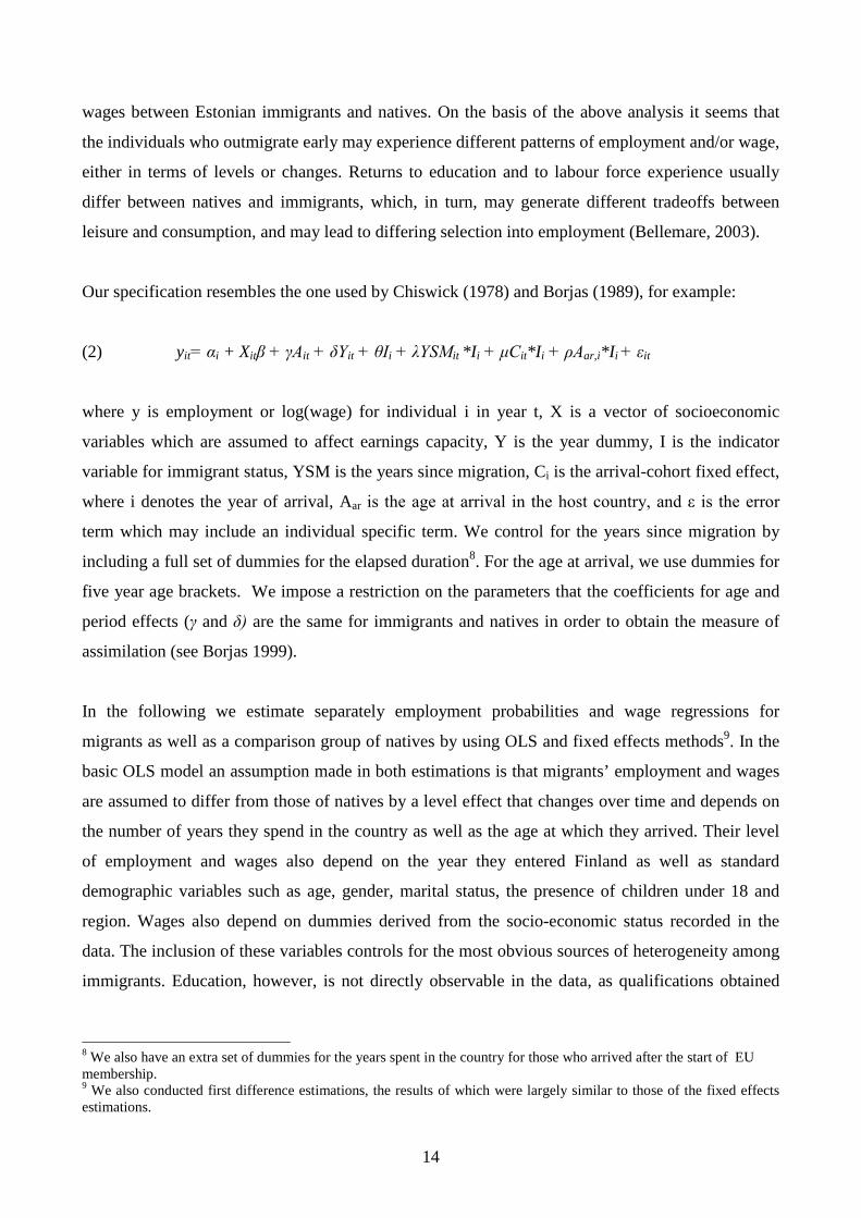
Our specification resembles the one used by Chiswick (1978) and Borjas (1989), for example:
(2) yit= αi + Xitβ + γAit + δYit + θIi + λYSMit *Ii + μCit*Ii + ρAar,i*Ii + εit
where y is employment or log(wage) for individual i in year t, X is a vector of socioeconomic
variables which are assumed to affect earnings capacity, Y is the year dummy, I is the indicator
variable for immigrant status, YSM is the years since migration, Ci is the arrival-cohort fixed effect,
where i denotes the year of arrival, Aar is the age at arrival in the host country, and ε is the error
term which may include an individual specific term. We control for the years since migration by
including a full set of dummies for the elapsed duration8. For the age at arrival, we use dummies for
five year age brackets. We impose a restriction on the parameters that the coefficients for age and
period effects (γ and δ) are the same for immigrants and natives in order to obtain the measure of
assimilation (see Borjas 1999).
In the following we estimate separately employment probabilities and wage regressions for
migrants as well as a comparison group of natives by using OLS and fixed effects methods9. In the
basic OLS model an assumption made in both estimations is that migrants’ employment and wages
are assumed to differ from those of natives by a level effect that changes over time and depends on
the number of years they spend in the country as well as the age at which they arrived. Their level
of employment and wages also depend on the year they entered Finland as well as standard
demographic variables such as age, gender, marital status, the presence of children under 18 and
region. Wages also depend on dummies derived from the socio-economic status recorded in the
data. The inclusion of these variables controls for the most obvious sources of heterogeneity among
immigrants. Education, however, is not directly observable in the data, as qualifications obtained
8 We also have an extra set of dummies for the years spent in the country for those who arrived after the start of EUmembership.9 We also conducted first difference estimations, the results of which were largely similar to those of the fixed effectsestimations.

15
abroad that most immigrants hold are not coded consistently. In addition, an interaction term of the
migrant dummy with gender is included in the equations.
With panel data, we are able to conduct both standard OLS regressions and fixed effect estimations where
individuals are compared to their own level of employment or wages, reflecting within individual changes
in these over time. There is no easy way to incorporate individual fixed effects into a non-linear
probability model. Therefore we use a linear probability model for the probability of employment10.
Naturally, differences in selection into employment may influence the migrant parameters of the
wage equation. In a cross-section, using the Heckman sample selection correction is the standard
way to control for possible differences in the selection process (see Dustmann and Rochina–
Barrachina 2007) and obtain correct estimates for the determinants of wages. This takes into
account the fact that we only observe wages for individuals whose wage exceeds their reservation
utility from working or, from the employers’ point of view, their expected productivity. In the case
of migrants this may, for example, lead to overestimating the wage gap between migrants and
natives, if migrants accept work for a lower wage. However, there is no single standard way to
implement the Heckman procedure with panel data, though various approaches have been proposed
(see, for example, Dustmann and Rochina–Barrachina 2007). They generally require further
assumptions to be made about the selection equation and the equation of interest. If the selection
term in wage equations arising from selection into employment is fixed over time, using panel
methods that remove fixed effects in the standard wage equation will solve the problem. With fixed
effects we are then able to trace the genuine within individual improvements in migrants’ wages
over time.
We do not have variables that could be used to instrument the decision to re-migrate in a wage or
employment equation. In order to analyse the impact that outmigration has on the estimates we run
each regression separately for the whole sample, and a sample that excludes those who are observed
to leave Finland. Both groups also include individuals who are future outmigrants but are not
identified as such. The results are also subject to limitations due to the length of the panel, the
longest durations represent only a few cohorts of immigrants. We, for example, observe the
individuals that arrived after the EU enlargement for a maximum of three years.
10 In order for the wage and employment equations to be consistent, we define ”employment” as having a higher thanzero labour-related income during year t.

16
For the employment equation the results from the OLS and fixed effects specifications are presented
in figures 5 and 6. The OLS estimate for the total employment gap is the sum of the coefficient of
Estonian nationality which indicates the employment difference between a migrant and a similar
native (effectively in the first year, as the difference to the latter years is controlled by further
dummies) and the coefficient of the corresponding later year of a migration spell. The gap also
depends on gender, the age at entry and the year of entry: in the coefficients presented in figures it
is implicitly assumed that this is at the base level or 19-24 years, and that the migrant is male and
entered in the year 200011. According to the OLS estimates, the migrants’ employment probability
increases compared to the initial significant gap (-26.7%) relative to natives but immediately after
the first year relatively slowly, in year three and four there is effectively no change. For the second
year, a part of the increase may be due to the fact that some of the new immigrants do not arrive at
the beginning of the year, and thus have less time to look for employment during their first year. A
slightly larger leap in employment takes place in year 5. The patterns of the coefficients for the
whole sample and the sample of stayers are very similar12.
A similar pattern can be observed for the estimates where the impact of individual levels has been
removed, or fixed effects estimates (figure 6). In the case of these estimates, we can naturally only
observe differences compared to migrants’ first year in Finland, and the interpretation of the
coefficient is not the total employment gap per se. The estimates, however, indicate whether
immigrants experience larger or smaller changes in employment rates compared to similar natives
during the course of their stay in Finland. The estimates in general are larger than zero, implying
that immigrants indeed improve their employment performance during the later years compared to
their first year and relative to what is, on average, the change of the employment rate for similar
natives.
The fixed effect estimates follow similar patterns for the whole sample as well as the sample of
stayers. Overall, the results indicate that while there are slight differences in the average
employment growth patterns of all migrants and the sample of stayers, the assimilation pattern of
employment rates is not qualitatively different in the two samples.
11 The coefficients for the year of entry are, by and large, insignificant, and the age of entry has a significant effectmainly in the older age groups.12 Strictly testing the equality of the coefficients from the two samples would require estimating a nested model.

17
Figure 5. OLS estimates of the employment gap and their 95% confidence intervals.
Figure 6. Fixed effects estimates (difference compared to the first year in Finland)and their 95% confidence intervals.
A comparison of the estimates obtained by using different methods provides further insight into
what extent immigrants’ employment growth in general is due to overall differences in employment
levels or different profiles for stayers. In figure 8 we explicitly compare the OLS coefficients and

18
those estimates where fixed effects or individual levels have been removed, taking only into
account the change in individual employment rates. The employment profiles for migrants are
slightly flatter when fixed effects have been removed or people are compared to their own initial
level of employment. However, there is still a rising employment profile.
Figure 7. Comparison of the OLS and fixed effects estimators of employmentassimilation.
The OLS results from wage estimations (Figure 8 and table 3 in the Appendix) for males who
arrived at the age of 30-34 show that wages grow slightly during the first years of migration spells,
but the increase becomes minimal or even negative after the fourth year. The initial wage
differential between natives and migrants, given that the individual is employed, depends heavily on
the age at arrival as well as gender, but the assimilation profile is constrained to be similar for all
individuals.
The results are very similar for both the whole sample and the sample restricted to stayers (see table
3 in the Appendix). The fixed effects estimates (figure 10 and table 3 in the Appendix) show similar
profiles that indicate an increase compared to the individual’s own initial wage level, but no
significantly higher total wage growth compared to natives over long durations.

19
Figure 8. Wage difference between natives and migrants who arrived at the age30-34 and its 95% confidence interval, OLS estimates.
Figure 9. Migrants’ wage difference compared to their first year in Finland, OLSand fixed effects estimates.
Overall, it seems that Estonian immigrants’ assimilation patterns observed in employment are
largely consistent with the traditional view of how migrants’ labour market performance improves
over time. For wages, there is an obvious initial gap between immigrants and natives for individuals
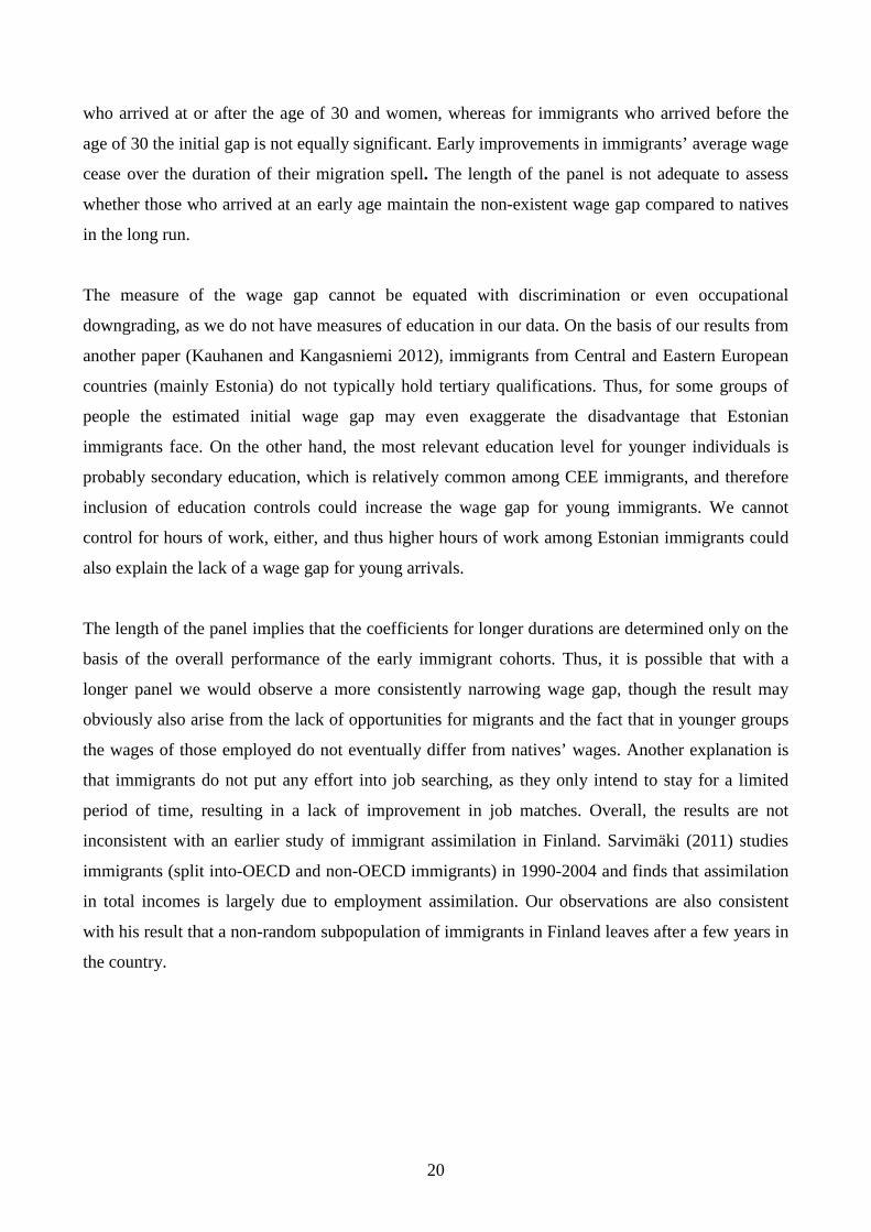
20
who arrived at or after the age of 30 and women, whereas for immigrants who arrived before the
age of 30 the initial gap is not equally significant. Early improvements in immigrants’ average wage
cease over the duration of their migration spell. The length of the panel is not adequate to assess
whether those who arrived at an early age maintain the non-existent wage gap compared to natives
in the long run.
The measure of the wage gap cannot be equated with discrimination or even occupational
downgrading, as we do not have measures of education in our data. On the basis of our results from
another paper (Kauhanen and Kangasniemi 2012), immigrants from Central and Eastern European
countries (mainly Estonia) do not typically hold tertiary qualifications. Thus, for some groups of
people the estimated initial wage gap may even exaggerate the disadvantage that Estonian
immigrants face. On the other hand, the most relevant education level for younger individuals is
probably secondary education, which is relatively common among CEE immigrants, and therefore
inclusion of education controls could increase the wage gap for young immigrants. We cannot
control for hours of work, either, and thus higher hours of work among Estonian immigrants could
also explain the lack of a wage gap for young arrivals.
The length of the panel implies that the coefficients for longer durations are determined only on the
basis of the overall performance of the early immigrant cohorts. Thus, it is possible that with a
longer panel we would observe a more consistently narrowing wage gap, though the result may
obviously also arise from the lack of opportunities for migrants and the fact that in younger groups
the wages of those employed do not eventually differ from natives’ wages. Another explanation is
that immigrants do not put any effort into job searching, as they only intend to stay for a limited
period of time, resulting in a lack of improvement in job matches. Overall, the results are not
inconsistent with an earlier study of immigrant assimilation in Finland. Sarvimäki (2011) studies
immigrants (split into-OECD and non-OECD immigrants) in 1990-2004 and finds that assimilation
in total incomes is largely due to employment assimilation. Our observations are also consistent
with his result that a non-random subpopulation of immigrants in Finland leaves after a few years in
the country.
21
6. Conclusions
The enlargement of the European Union initiated almost unrestrained flows of migration from
Central and Eastern European countries to Western Europe. This has raised concerns about the
burden Eastern European immigrants place on welfare states. These migration flows have also
proved to be circular: some of the migrants return to their home countries after just a few years in
the host country. The circular pattern of migration may have important implications for the
consequences of migration flows on the whole. In this paper we have tried to establish some facts
regarding the re-migration and assimilation of Estonian immigrants in Finland in 2000-2007.
During this period Estonia joined the EU, and the data also allow us to observe changes in
outmigration patterns as a result of membership.
Our descriptive analysis suggests that those who outmigrate experience a lower level of
employment and weaker labour force attachment. Our survival analysis indicates that higher
monthly labour-related earnings have a negative coefficient when interacted with the early years of
migration spells, but these coefficients cease to be significant when the duration of a spell exceeds
five years. The regression analysis on immigrant assimilation reveals that, controlling for
background characteristics, the immigrants’ employment rate increases even in the last years of the
longest spells observed, but with little change in some of the earlier years. As for wages, the initial
wage gap depends on the age of arrival and gender and during the first few years of migration spells
employed immigrants experience wage growth, but with longer spells there is no equally significant
difference compared to the migrants’ first year in Finland. Excluding the identified outmigrants
does not qualitatively change the patterns of assimilation: despite obviously non-random
outmigration we also observe genuine improvement in employment and wage outcomes for those
who are not observed to leave the sample.
22
Literature
Bellemare, C. (2003), Identification and estimation of economic models of outmigration using panel
attrition. IZA Discussion paper No. 1065.
Borjas, G. J. (1985), Assimilation, changes in cohort quality, and the earnings of immigrants.
Journal of Labor Economics 3, 463-489.
Borjas, G. J. (1989), Immigrant and Emigrant Earnings: A Longitudinal Study. Economic Inquiry
27(1), 21-37.
Borjas, G. J. (1999), The Economic Analysis of Immigration, In (D. Card and O. Ashenfelter
(eds.)), Handbook of Labor Economics, Vol. 3, Amsterdam: North-Holland.
Borjas, G. J. and Bratsberg, B. (1996), Who Leaves? The Outmigration of the Foreign-Born. The
Review of Economic and Statistics 78(1), 165-176.
Chiswick, B. (1978), The Effect of Americanization on the Earnings of Foreign-born Men. The
Journal of Political Economy 86(5), 897-921.
Chiswick, B. R., Lee Y. L., Miller, P. W. (2002), Longitudinal Analysis of Immigrant Occupational
Mobility: A Test of the Immigrant Assimilation Hypothesis. IZA Discussion Paper No. 452.
Constant, A. and Massey, D. (2003), Self-Selection, Earnings, and Out-Migration: A Longitudinal
Study of Immigrants to Germany. Journal of Population Economics 16(?), 631-653.
Duleep, H. and Dowhan, D. (2002), Insights from longitudinal data on the earnings growth of U.S.
foreign-born men. Demography 39(3), 485-506.
Dustmann, C. (2003a), Return Migration, Wage Differentials, and the Optimal Migration Duration.
European Economic Review, Vol. 47, 353-369.
Dustmann, C. (2003b), Children and Return Migration. Journal of Population Economics, Vol. 16,
815-830.
Edin, P-A., LaLonde, R. and Åslund, O. (2000), Emigration of Immigrants and Measures of
immigrant Assimilation: Evidence from Sweden. Swedish Economic Policy Review 7, 163-
204.
Fertig, M. and Schurer, S. (2007), Labour Market Outcomes of Immigrants in Germany: The
importance of Heterogeneity and Attrition Bias. IZA Discussion paper 2915.
Friedberg, R. M. (1992), The Labor market assimilation of immigrants in the United States: The
role of age at arrival. Mimeo (December 1992), Brown University.
Hu, W.-Y. (2000), Immigrant earnings assimilation: estimates from longitudinal data. The
American Economic Review Papers and Proceedings of the One Hundred Twelfth Annual
Meeting of the American Economic Association, Vol. 90, 368–372.
23
Hum, D. and Simpson, W. (2004), Reinterpreting the performance of immigrant wages from panel
data. Empirical Economics 29, 129-47.
Kaushal, N. (2011), Earning Trajectories of Highly Educated Immigrants: Does Place of Education
Matter? Industrial & Labor Relations Review, Vol. 64, No. 2, 323-340.
Krusell, S. (2009), Employment of Estonian Residents Abroad. Eesti Statistika Kvartalikiri –
Quarterly Bulletin of Statistics Estonia 2/09, 63-74.
LaLonde, R. and Topel, R. (1992), The Assimilation of Immigrants in the U.S. Labor Market. In G.
Borjas and R. Freeman (eds.), Immigration and the Work Force, 67–92, Chicago: University
of Chicago Press.
Longva, P. (2001), Out-Migration of Immigrants: Implications for Assimilation Analysis.
Memorandum, No. 4, Department of Economics, University of Oslo.
Lubotsky (2007), Chutes or Ladders? A Longitudinal Analysis of Immigrant Earnings. Journal of
Political Economy, Vol. 115, No. 5, 820-867.
Mesnard, A. (2004), Temporary Migration and Capital Market Imperfections. Oxford Economic
Papers, Vol. 56, 242-262.
Picot, G. and Piraino, P. (2011), Immigrant Earnings Growth: Selection Bias or Real Progress?
Canadian Labour Market and Skills Researcher Network Working Paper No. 69.
Reagan, P. B. and Olsen, R. J. (2000), You Can Go Home Again: Evidence from Longitudinal
Data. Demography 37(3), 339–350.
Sarvimäki, M. (2011), "Assimilation to a Welfare State: Labor Market Performance and Use of
Social Benefits by Immigrants to Finland." Scandinavian Journal of Economics, Wiley
Blackwell, Vol. 113(3), 665-688, 09.

24
Table 1. Descriptive statistics of characteristics of Finnish natives, all Estonian immigrants andimmigrants subdivided into stayers and outmigrants during 2000-2007 – means and standarddeviations (in the brackets).
Variable Natives Estonianimmigrants
Outmigrants Stayers
Female 0.496(0.499)
0.509(0.499)
0.366(0.482)
0.523(0.499)
Age (average) 41.4(13.2)
36.6(10.54)
35.0(10.92)
36.7(10.51)
Age at entry (average) - 34.7(10.47)
33.7(10.79)
34.8(10.43)
Age group:
Age 18-24 0.140(0.347)
0.123(0.329)
0.166(0.372)
0.12(0.325)
Age 25-54 0.665(0.475)
0.819(0.384)
0.763(0.425)
0.824(0.380)
Age 55-64 0.204(0.403)
0.057(0.231)
0.07(0.257)
0.05(0.229)
Married 0.474(0.499)
0.438(0.496)
0.338(0.473)
0.447(0.497)
Children under 18 0.352(0.477)
0.309(0.462)
0.20(0.400)
0.32(0.466)
Socioeconomic status:
Entrepreneur 0.047 0.038 0.02 0.039
Upper white-collar worker 0.091 0.049 0.04 0.050
Lower white-collar worker 0.152 0.082 0.05 0.086
Blue-collar worker 0.148 0.412 0.277 0.424
Other 0.186 0.204 0.152 0.208
Socio-economic status is missing 0.375 0.214 0.457 0.192
Monthly earnings (average for thewhole period) (>0)
2311.5(22.65)
2041.4(17.17)
2031.1(18.09)
2042.2(17.10)
Monthly earnings (average for thewhole period) (including zeroes)
1788.6(22.12)
1428.1(17.14)
1177.4(22.12
1450.6(17.13)
Annual earnings quartiles by meanearnings for the whole period1)
1 21.5 27.4 38.0 26.5
2 25.0 36.9 33.4 37.2
3 26.4 21.5 17.1 21.9
4 27.0 14.1 11.2 14.3
Average number of workingmonths per year for the wholeperiod
10.2(3.39)
8.93(3.87)
7.75(4.11)
9.02(3.84)
Number of observations 127,824 12,658 1,042 11,616

25
Appendix
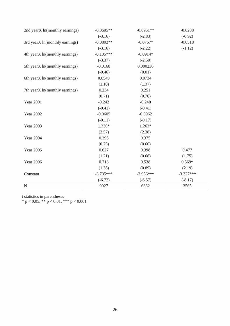
Table 1. Coefficient estimates of the complementary log-log hazard of outmigration
(1) (2) (3)
All Arrival before 2004 Arrival after 2004
Unemployment benefit paid -0.931** -0.553 -2.572*
(-3.12) (-1.62) (-2.49)
Entrepreneur -0.223 -1.228 0.926*
(-0.58) (-1.71) (1.97)
Low white collar -0.252 -0.537 0.00210
(-0.84) (-1.16) (0.01)
High white collar -0.0645 -0.491 0.346
(-0.26) (-1.31) (1.06)
Age at entry -0.00181 -0.00270 -0.000485
(-0.37) (-0.41) (-0.06)
Outside labour force 0.590*** 0.524* 0.700**
(3.57) (2.40) (2.82)
Married -0.311* -0.264 -0.276
(-2.04) (-1.41) (-1.03)
MarriedXFemale -0.330 -0.366 -0.552
(-1.40) (-1.27) (-1.22)
Female -0.279* -0.172 -0.431*
(-2.07) (-0.93) (-2.15)
Children under 18 -0.721** -0.996** -0.500
(-3.24) (-2.99) (-1.66)
FemaleX Children under 18 0.580* 0.954* 0.246
(2.01) (2.36) (0.57)
log(benefits) -0.0537*** -0.0735*** -0.0289
(-3.64) (-3.71) (-1.31)
log(monthly earnings) -0.00198 -0.0139 0.00188
(-0.11) (-0.51) (0.08)
2nd year -0.219 -0.184 -0.306
(-1.52) (-0.75) (-1.57)
3rd year -0.485** -0.225 -0.788*
(-2.72) (-0.86) (-2.45)
4th year -0.557* -0.300
(-2.37) (-0.96)
5th year -0.172 0.161
(-0.74) (0.46)
6th year -0.0153 0.349
(-0.06) (0.89)
7th year -1.181 -0.829
(-1.05) (-0.71)
26
2nd yearX ln(monthly earnings) -0.0695** -0.0951** -0.0288
(-3.16) (-2.83) (-0.92)
3rd yearX ln(monthly earnings) -0.0802** -0.0757* -0.0518
(-3.16) (-2.22) (-1.12)
4th yearX ln(monthly earnings) -0.105*** -0.0914*
(-3.37) (-2.50)
5th yearX ln(monthly earnings) -0.0168 0.000236
(-0.46) (0.01)
6th yearX ln(monthly earnings) 0.0549 0.0734
(1.10) (1.37)
7th yearX ln(monthly earnings) 0.234 0.251
(0.71) (0.76)
Year 2001 -0.242 -0.248
(-0.41) (-0.41)
Year 2002 -0.0605 -0.0962
(-0.11) (-0.17)
Year 2003 1.330* 1.263*
(2.57) (2.38)
Year 2004 0.395 0.375
(0.75) (0.66)
Year 2005 0.627 0.398 0.477
(1.21) (0.68) (1.75)
Year 2006 0.713 0.538 0.569*
(1.38) (0.89) (2.19)
Constant -3.735*** -3.956*** -3.327***
(-6.72) (-6.57) (-8.17)
N 9927 6362 3565
t statistics in parentheses* p < 0.05, ** p < 0.01, *** p < 0.001

27
Table 2. Coefficient estimates of the linear probability of having labour-related income
OLS, All FE, All OLS, Only stayers FE, Only stayers
Prob(Monthlylabour-relatedearnings>0)
Prob(Monthlylabour-relatedearnings>0)
Prob(Monthlylabour-relatedearnings>0)
Prob(Monthlylabour-relatedearnings>0)
Year 2001 0.009*** -0.004 0.009*** -0.004
(3.30) (-1.37) (3.36) (-1.37)
Year 2002 0.010** -0.013*** 0.010*** -0.013***
(3.21) (-3.72) (3.30) (-3.73)
Year 2003 0.005 -0.024*** 0.006 -0.024***
(1.54) (-6.24) (1.76) (-6.16)
Year 2004 0.005 -0.029*** 0.005 -0.029***
(1.60) (-6.70) (1.43) (-6.78)
Year 2005 -0.004 -0.042*** -0.004 -0.042***
(-1.16) (-8.69) (-1.13) (-8.73)
Year 2006 0.000 -0.042*** 0.000 -0.042***
(0.01) (-7.84) (0.13) (-7.87)
Estonian -0.269*** . -0.256*** .
(-8.53) . (-7.68) .
Year of entry 2001 0.052 . 0.054 .
(1.78) . (1.74) .
Year of entry 2002 0.029 . 0.034 .
(0.94) . (1.05) .
Year of entry 2003 0.077* . 0.051 .
(2.44) . (1.51) .
Year of entry 2004 0.005 . -0.002 .
(0.01) . (-0.01) .
Year of entry 2005 0.001 . -0.018 .
(0.00) . (-0.05) .
Year of entry 2006 0.089 . 0.076 .
(0.26) . (0.23) .
Age at entry 1518 0.049 . 0.031 .
(1.10) . (0.67) .
Age at entry 2529 -0.002 . -0.006 .
(-0.07) . (-0.24) .
Age at entry 3034 0.020 . 0.022 .
(0.75) . (0.79) .
Age at entry 3539 0.037 . 0.035 .
(1.40) . (1.27) .
Age at entry 4044 0.030 . 0.020 .
(1.10) . (0.71) .
Age at entry 4550 0.101*** . 0.092** .
(3.58) . (3.11) .

28
Age at entry 50 over 0.165*** . 0.153*** .
(5.26) . (4.61) .
Age_1518 -0.461*** -0.344*** -0.460*** -0.345***
(-51.44) (-21.24) (-51.24) (-21.31)
Age _1924 -0.041*** -0.110*** -0.040*** -0.110***
(-5.27) (-9.67) (-5.14) (-9.72)
Age _2529 0.009 -0.049*** 0.010 -0.049***
(1.29) (-6.42) (1.51) (-6.40)
Age _3539 0.010 0.052*** 0.011 0.053***
(1.57) (7.59) (1.74) (7.67)
Age _4044 0.015* 0.089*** 0.016* 0.090***
(2.03) (9.00) (2.12) (9.09)
Age _4549 -0.007 0.108*** -0.007 0.108***
(-0.93) (8.61) (-0.87) (8.68)
Age _5054 -0.057*** 0.105*** -0.056*** 0.106***
(-6.99) (7.03) (-6.89) (7.06)
Age _5559 -0.185*** 0.064*** -0.184*** 0.065***
(-19.85) (3.66) (-19.81) (3.73)
Age _60yli -0.612*** -0.084*** -0.612*** -0.083***
(-67.63) (-4.13) (-67.60) (-4.08)
Region_2 -0.025** -0.064** -0.025** -0.064**
(-3.05) (-3.14) (-3.09) (-3.14)
Region _3 -0.042*** -0.061** -0.043*** -0.060**
(-5.31) (-3.03) (-5.40) (-2.99)
Region _4 -0.055*** -0.080*** -0.056*** -0.080***
(-11.24) (-6.67) (-11.36) (-6.61)
Female 0.053*** . 0.053*** .
(7.71) . (7.68) .
Female&Estonian -0.162*** . -0.158*** .
(-10.63) . (-10.02) .
Married 0.106*** 0.019* 0.107*** 0.019*
(16.07) (2.40) (16.18) (2.41)
Female&Married -0.077*** -0.031* -0.077*** -0.030*
(-9.09) (-2.46) (-9.04) (-2.41)
Children under 18 0.048*** -0.021*** 0.047*** -0.021***
(8.26) (-3.34) (8.09) (-3.40)
Female&Childrenunder 18
-0.096*** -0.061*** -0.095*** -0.061***
(-12.15) (-6.43) (-12.11) (-6.38)
2nd year 0.092*** 0.096*** 0.111*** 0.116***
(7.66) (7.35) (8.61) (8.24)
3rd year 0.087*** 0.084*** 0.105*** 0.111***
(5.78) (5.10) (6.61) (6.39)
4th year 0.102*** 0.086*** 0.111*** 0.113***
(6.17) (4.81) (6.45) (6.02)

29
5th year 0.181*** 0.146*** 0.173*** 0.169***
(9.67) (7.16) (8.86) (8.05)
6th year 0.195*** 0.153*** 0.185*** 0.177***
(8.30) (6.01) (7.58) (6.72)
7th year 0.260*** 0.217*** 0.245*** 0.234***
(7.22) (5.51) (6.67) (5.87)
1st year for arrivalsafter EU
0.166 0.057* 0.171 0.082**
(0.49) (2.13) (0.51) (2.99)
2nd year for arrivalsafter EU
0.125 0.011 0.115 0.021
(0.37) (0.52) (0.34) (0.96)
3rd year for arrivalsafter EU
0.109 0.093
(0.32) (0.28)
_cons 0.827*** 0.807*** 0.826*** 0.807***
(103.86) (72.72) (103.60) (72.51)
N 133720 133720 132753 132753
t statistics in parentheses* p < 0.05, ** p < 0.01, *** p < 0.001

30
Table 3. Coefficient estimates of the wage regression
All, OLS All, FE Only stayers, OLS Only stayers, FE
Log(wage) Log(wage) Log(wage) Log(wage)
Year 2001 0.033*** 0.005 0.033*** 0.005
(5.29) (0.92) (5.24) (0.89)
Year 2002 0.025*** -0.021*** 0.025*** -0.021***
(3.70) (-3.66) (3.74) (-3.59)
Year 2003 0.058*** -0.006 0.058*** -0.006
(7.98) (-0.94) (7.98) (-0.97)
Year 2004 0.068*** 0.004 0.068*** 0.004
(9.13) (0.60) (9.18) (0.64)
Year 2005 0.084*** -0.009 0.083*** -0.009
(11.26) (-1.81) (11.24) (-1.79)
Year 2006 0.103*** . 0.103*** .
(13.61) . (13.58) .
Estonian 0.037 . 0.033 .
(0.70) . (0.59) .
Year of entry 2001 0.086 . 0.077 .
(1.87) . (1.61) .
Year of entry 2002 0.038 . 0.036 .
(0.79) . (0.73) .
Year of entry 2003 0.021 . 0.024 .
(0.42) . (0.45) .
Year of entry 2004 0.663*** . 0.637*** .
(10.31) . (9.51) .
Year of entry 2005 0.687*** . 0.663*** .
(10.72) . (9.98) .
Year of entry 2006 0.637*** . 0.631*** .
(11.97) . (11.20) .
Age at entry 1518 -0.130 . -0.129 .
(-1.64) . (-1.57) .
Age at entry 2529 -0.044 . -0.033 .
(-1.06) . (-0.75) .
Age at entry 3034 -0.197*** . -0.203*** .
(-4.64) . (-4.61) .
Age at entry 3539 -0.312*** . -0.306*** .
(-7.52) . (-7.12) .
Age at entry 4044 -0.331*** . -0.337*** .
(-8.02) . (-7.83) .
Age at entry 4550 -0.344*** . -0.349*** .
(-7.99) . (-7.82) .
Age at entry 50 over -0.190*** . -0.201*** .
(-4.11) . (-4.14) .

31
Age 0.129*** 0.182*** 0.130*** 0.182***
(48.22) (35.21) (48.17) (35.28)
Age squared -0.001*** -0.002*** -0.001*** -0.002***
(-41.75) (-29.85) (-41.72) (-29.92)
Region_2 -0.065*** -0.042 -0.067*** -0.044
(-4.54) (-0.91) (-4.63) (-0.95)
Region _3 -0.064*** -0.065 -0.064*** -0.066
(-4.34) (-1.57) (-4.36) (-1.59)
Region _4 -0.108*** -0.135*** -0.109*** -0.139***
(-11.81) (-4.89) (-11.87) (-5.01)
Entrepreneur -0.304*** -0.190*** -0.305*** -0.192***
(-13.10) (-5.21) (-13.12) (-5.24)
Upper white collar 0.545*** 0.093*** 0.545*** 0.092***
(49.42) (6.01) (49.30) (6.00)
Lower white collar 0.229*** 0.060*** 0.230*** 0.060***
(27.80) (5.08) (27.90) (5.10)
Female -0.207*** . -0.207*** .
(-17.26) . (-17.24) .
FemaleXEstonian -0.144*** . -0.145*** .
(-5.97) . (-5.86) .
Married 0.141*** 0.010 0.141*** 0.009
(11.53) (0.61) (11.47) (0.59)
FemaleXMarried -0.138*** -0.071** -0.138*** -0.073**
(-8.54) (-2.70) (-8.50) (-2.79)
Children under 18 -0.028* -0.061*** -0.028* -0.061***
(-2.48) (-4.83) (-2.49) (-4.83)
FemaleX Childrenunder 18
-0.127*** -0.169*** -0.128*** -0.168***
(-8.08) (-8.38) (-8.11) (-8.33)
2nd year 0.046 0.051 0.056* 0.056
(1.84) (1.83) (2.09) (1.89)
3rd year 0.083** 0.082* 0.089** 0.083*
(2.71) (2.47) (2.70) (2.31)
4th year 0.110*** 0.083* 0.122*** 0.088*
(3.66) (2.47) (3.83) (2.47)
5th year 0.096** 0.083* 0.106** 0.085*
(2.82) (2.17) (2.92) (2.10)
6th year 0.081 0.058 0.096* 0.065
(1.89) (1.29) (2.17) (1.44)
7th year 0.032 -0.001 0.037 -0.004
(0.49) (-0.01) (0.55) (-0.05)
1st year for arrivalsafter EU
-0.578*** 0.006 -0.554*** 0.004
(-15.21) (0.12) (-14.37) (0.08)

32
2nd year for arrivalsafter EU
-0.579*** 0.005 -0.558*** -0.003
(-11.28) (0.14) (-10.54) (-0.07)
3rd year for arrivalsafter EU
-0.591*** -0.551***
(-9.51) (-8.72)
_cons 0.294*** -1.057*** 0.294*** -1.058***
(6.25) (-9.88) (6.24) (-9.88)
N 95318 95318 94768 94768