Where will efficient energy release occur in 3D

magnetic configurations?

P. Demoulin

Observatoire de Paris, section de Meudon, LESIA, UMR 8109 (CNRS), F-92195Meudon Cedex, France

Abstract

The energy needed to power flares is thought to be stored in the coronal magneticfield. However, the energy release is efficient only at very small scales. Magneticconfigurations with a complex topology, i.e. with separatrices, are the most obviousconfigurations where current sheets can form, and then, reconnection can efficientlyoccur. This has been confirmed for several flares computing the coronal field andcomparing the locations of the flare loops and ribbons to the deduced 3D magnetictopology. However, this view is too restrictive taking into account the variety ofobserved solar flaring configurations. Indeed, “Quasi-Separatrix Layers” (QSLs),which are regions where there is a drastic change in field-line linkage, generalize thedefinition of separatrices. They let us understand where reconnection occurs in abroader variety of flares than separatrices do. The strongest electric field and currentare generated at, or close to where the QSLs are thinnest. This defines the regionwhere particle acceleration can efficiently occur. A new feature of 3-D reconnectionis the natural presence of fast field line slippage along the QSLs, a process called“slip-running reconnection”. This is a plausible origin for the motions of the X-raysources along flare ribbons.

Key words: Magnetic Reconnection, Sun: magnetic fields, Sun: X-rays, Sun: flares

1 Introduction

The solar corona is formed by a low-β plasma where the magnetic field has akey role. One of the best examples are flares, where a large amount of mag-netic energy is released, and the creation of new magnetic connectivities canbe directly seen as flare loops. The progression of flare ribbons traces thedisplacement of the energy released location in the magnetic configuration(the ribbons are the mapping image, along field lines, of the energy releasein the corona). However, the observations provide mostly informations on the

Preprint submitted to Elsevier Science 29 January 2007

consequences of magnetic energy release (as emission of heated plasma andradiation from accelerated particles, with small delays due to the energy trans-port processes). An important investigation work is needed to assemble all theobservational facts to constrain the energy release mechanism.

It is striking to see, at a given time in a flare, how localized are the traces ofenergy release (ribbons, new flare loops). This shows that special conditions areneeded to transform the stored magnetic energy. Indeed, there is an expectedvery low dissipation of the coronal field at the spatial scales of the global flaringconfiguration (typically an active region). The resistive term in the inductionequation can become large enough only if narrow current layers are created.This is the origin of the spatial localization of the energy release in flares.

Current sheets can form easily along separatrices both in 2-D and 3-D configu-rations. The concept of separatrices has been generalized in 3-D configurationsto QSLs and the theory was successfully tested with multi-wavelength observa-tions of flares and less energetic events (Section 2). Why and how current layersare formed along Quasi-Separatrix Layers (QSLs) is summarized in Section 3.Then, the recent developments of 3-D magnetic reconnection are summarized,and set in the perspective of X-ray observations (Section 4). Finally, some ofthe remaining challenges theory has to face are discussed in Section 5.

2 Separatrices and QSLs

Separatrices are magnetic surfaces where the magnetic field line linkage isdiscontinuous. The simplest example is a 2-D magnetic configuration with anX-point or null point (where the magnetic field vanishes). Two separatricescross at the X-point, and they define four separated regions, called connectiv-

ity domains, where the magnetic connectivity changes continuously from onefield line to its neighbor, but discontinously at the boundaries of the domains(separatrices).

The above 2-D concepts have been generalized to 3-D null points. The vicin-ity of a null point is described by the linear term in the local Taylor expan-sion of the magnetic field. The diagonalisation of the field’s Jacobian matrixprovides three orthogonal eigenvectors (Molodenskii and Syrovatskii, 1977).The divergence-free condition imposes that the sum of the three eigenvaluesvanishes (λ1 + λ2 + λ3 = 0), and for magnetic fields in equilibrium with a

plasma (~j × ~B = ~∇P ) the eigenvalues are real (Lau and Finn, 1990). Thentwo eigenvalues, say λ1, λ2, have the same sign, opposite to the one of thethird eigenvalue λ3. The two eigenvalue field lines, which start from an in-finitesimal distance of the null in directions parallel and anti-parallel to theeigenvector associated to λ3, are called γ-lines, or spines. The separatrix,

2

called Σ-surface or fan, is defined by all the field lines starting at an in-finitesimal distance of the null in the plane defined by the two eigenvectorsassociated to λ1 and λ2. The γ-lines/spines and Σ-surface/fan are defined bythe local properties of the null, but they have large scale implications for thetopology of the magnetic field.

Two types of 3-D nulls exist depending on the sign of the Σ-surface/fan eigen-values; their sign is used to define the sign of the null. A more complex topol-ogy is build with two “interacting” nulls of opposite signs, called A and B.The intersection of the fans (ΣA and ΣB) define a magnetic null-null line

or separator. The separatrices of the configuration are the two surfaces ΣA

and ΣB bounded by the γ-lines (giving the possibility to have unclosed sep-aratrices, Lau, 1993). The complexity of the field topology increases rapidlywith the number of nulls present. Longcope and Klapper (2002) provided ageneral theoretical framework to analyze the frequently very complex mag-netic topology of 3-D configurations formed by many flux tubes (as observedin magnetograms).

An important location for current-sheet formation, then, for reconnection ina classical view, is the intersection of two separatrices, which is a null point in2-D and a separator in 3-D (Gorbachev and Somov, 1988; Lau and Finn, 1990;Longcope and Cowley, 1996). More generally, current sheets are thought toform all along the separatrices when arbitrary motions are imposed at theirintersection with the lower line-tied boundary (e.g. Zwingmann et al., 1985;Low and Wolfson, 1988; Aly, 1990; Lau, 1993; Yokoyama and Shibata, 1994).For further information see the review of Longcope (2005).

Some of the studied flaring active regions (ARs) have indeed, at least, onemagnetic null point in the extrapolated coronal fields (e.g. Mandrini et al.,1993; Gaizauskas et al., 1998; Longcope and Silva, 1998; Aulanier et al., 2000;Fletcher et al., 2001b; Longcope et al., 2005; Mandrini et al., 2006). These flareanalyses have shown that Hα and UV flare ribbons are typically located at, orin the close vicinity of, the intersection of separatrices with the chromosphere.The ribbons are connected by field lines (computed from magnetic field ex-trapolations). These results provide evidence that flares are a consequence oflocalized magnetic reconnection in the corona.

Separatrices are also present when dipped field lines are tangent to the photo-spheric boundary. The bottom of these local magnetic dips are called ”bald

patches” (Titov et al., 1993). Pariat et al. (2004) found that reconnection atbald-patch separatrices is a key process during the emergence of magnetic fluxthrough the photosphere, since this reconnection process allows the release ofthe dense plasma caught in the magnetic dips (it removes the plasma weight),and so it allows the magnetic field to cross the photosphere. Moreover, thecomputed bald patch topology let us understand the morphology of several

3

Fig. 1. Illustration of the QSLs in one of the simplest magnetic configurations(formed by two potential magnetic bipoles). The greyscale images show the dis-tribution of the squashing degree Q at the lower boundary in logarithmic scale(white: Q = 6, black: Q = 1011). Two sets of field lines are shown in order to visual-ize the drastic change of connectivity, both sets have footpoints starting in a shortsegment crossing one QSL at the lower boundary. Continuous and dashed contoursshow positive and negative values of the vertical field component, respectively (fromAulanier et al., 2005).

small eruptive events (Aulanier et al., 1998; Mandrini et al., 2002), transitionregion brightenings (Fletcher et al., 2001a), and some interconnecting arcsbetween two ARs (Delannee and Aulanier, 1999).

In summary, there are many observed cases where the separatrices of coronalnull points or bald patches let us understand the spatial localization of theenergy release. However, in several ARs no such coronal null point, or baldpatch, can be found and linked to the observational evidences of energy release(Demoulin et al., 1994). Of course, it is possible that the model of the coronalfield is not close enough to the real field, but it was shown that a broaderconcept than separatrices can help us to understand the observed traces ofenergy release, using the same magnetic extrapolation methods, as explainedbelow.

To address the difficulties of interpreting several flares with only separatri-ces, Demoulin et al. (1996a,b) proposed that “quasi-separatrix layers” (QSLs)generalize the definition of separatrices to cases where there is no coronal mag-netic null and no bald patch. QSLs are regions where there is a drastic changein field line linkage (Fig. 1). The drastic change in linkage can be quantifiedusing Q, called the squashing degree (computed from spatial derivatives onthe magnetic connections). Then, a QSL is present at locations where Q >> 2(Titov et al., 2002).

Let us consider a tiny circular region in one photospheric magnetic polarity.Outside QSLs, this region is mapped following field lines to a region in theother polarity which could have a complex shape, but comparable extensionsin all directions. However, if the circular region is inside a QSL, it is mapped

4

to a very elongated and flatten region, ellipsoidal-like, in the other polarity.The squashing degree, Q, measures the aspect ratio of this ellipse; in otherwords, how much the initial region is squashed by the field-line mapping. Q

can take very high values, by many orders of magnitudes.

QSLs include, as a the limit case when Q → ∞, the concept of separatrices.With separatrices the mapping changes so drastically that it is discontinuous.Let us consider a potential magnetic configuration, as in Fig. 1, formed byfour magnetic concentrations at the lower boundary (e.g. photospheric level),with a normal field component, Bn, vanishing only along a line, called theinversion line. Unless the two magnetic bipoles are close to be anti-parallel,there is generally no magnetic null above the lower boundary and the mag-netic connectivity is continuous, but drastically changing at the QSLs. Letus transform progressively the magnetic configuration by concentrating moreand more the magnetic field in the four magnetic concentrations at the lowerboundary, keeping their center of gravity at the same locations. For simplicityof the illustration, let us keep the configuration potential. As the field concen-tration increases, the QSLs stay basically at the same locations while they getthinner (Q increases, Demoulin et al., 1996a). When the field concentration islarge enough, Q becomes infinite: the QSLs becomes separatrices associatedto at least one null present first at the lower boundary (and eventually in thevolume). More generally, QSLs converge to separatrices in the limit where thephotospheric unipolar regions are separated by flux free regions (Bn = 0).Then, analyzing QSLs permit to detect “topological” features of the magneticfield which could be related to separatrices in some limit case of the model.However, many magnetic configurations have no separatrix but they do haveQSLs. The relationship between separatrices and QSLs is further analyzed inthe reviews by Demoulin (2005) and Longcope (2005).

At any given region inside QSLs, two field lines, which are locally close by,diverge from each other when computed away from this region. This effect isstrongest in the central part of QSLs, where the strongest mapping distortionsare present (largest Q values). The way field lines diverge from each othersuggests that we call the central part of the QSLs a hyperbolic flux tube

(HFT, Titov et al., 2002). The HFT generalizes the concept of separator: asabove for QSLs, when the boundary field get more and more concentrated,the region with the highest Q-values converge to a null-null line (if two nullpoints are present in the volume) or to a quasi null line (if only one null ispresent, Lau, 1993). However, like above with QSLs, an HFT can be presentwithout null point in the magnetic configuration considered. The theoreticaldevelopments on QSLs and HFTs have been reviewed in Titov (2005) andDemoulin (2006).

For each studied flare, the flare ribbons were always found along, or justnearby, the intersection of QSLs with the chromosphere (e.g. Demoulin et al.,

5

R2 N R3R1 R4 R2 R3R1 R4Fig. 2. Flaring processes one hour before the X17 flare on October 28, 2003. Leftpanel: TRACE image in 1600 A in reverse intensity scale. The main ribbons (darkregions) are labeled (R1, R2, R3, R4). The position of the only magnetic null pointfound in the extrapolation of the photospheric field is marked with an N. Recon-nection there can only explain the brightenings seen in its close vicinity (withoutlabels), but not the four main ribbons. Right panel: Drastic change of coronal con-nectivities, so QSLs, are found at or in the close vicinity of the four main ribbons.They are the result of energy release by magnetic reconnection at QSLs (notice thatthe null point, N, is very low in the atmosphere, and it is not related to the X-likeconfiguration of the field lines as seen in projection). The axes are labeled in Mmand the isocontours of the field correspond to ± 100 and ± 1000 G in continuous(dashed) style for the positive (negative) values (from Mandrini et al., 2006).

1997; Mandrini et al., 1997; Bagala et al., 2000). Other examples are reviewedby Demoulin (2006). These results demonstrate that flares are coronal events,where the release of free magnetic energy is due to the presence of regionswhere the magnetic field line linkage changes drastically, and not necessarilydiscontinuously.

A flare example involving both separatrices and QSLs is given in Fig. 2. Onlyone magnetic null point was found in the extrapolated field; it was located ata height of only ≈ 4000 km above the magnetogram location (Mandrini et al.,2006). The photospheric trace of the separatrices are in the close vicinity of thebrightenings observed near the null point (towards the north and south, at adistance ≤ 20 Mm, and towards the east, at a distance ≤ 40 Mm). Moreover,the field lines in the vicinity of the null point let us understand the shapeand location of the coronal loops observed by TRACE in terms of classicalreconnection at a null point. Similar coronal loops were present before andafter the X17 flare showing that this localized reconnection is independentof the main flare. Before the X17 flare, four bright ribbons were also present(Fig. 2, left). They can be linked by field lines in a quadrupolar configuration(Fig. 2, right). A classical approach, considering only null points and baldpatches, is not able to explain the presence of these four ribbons. Howeverthis reconnection before the X17 flare can be readily interpreted with QSLs.This is an example of a precursor that contributes to the launch of the main

6

eruptive flare (X17).

3 Formation of electric current layers

The formation of a strong current layer in any QSL is expected with almostany kind of boundary motion across the QSL, as conjectured analyticallyby Demoulin et al. (1996a). The main reason is that the magnetic stressof very distant regions, generated by plasma flows, can be brought close toone another, typically over the QSL thickness (the magnetic stress is mainlytransported by Alfven waves which are damped later in the quasi-equilibriumstate).

MHD numerical simulations are required to analyze the evolution of generalmagnetic configurations having QSLs. A numerical difficulty is that the cur-rents are expected to form on the scale of the QSL thickness, a scale that canbe many orders of magnitude lower than the global scale of the studied mag-netic configuration. In a simulation the thinnest scales are limited by the sizeof the numerical cells. All the current layers should be broader; this is attainedby selecting a resistivity large enough. The MHD simulations of Longcope andStrauss (1994) and Milano et al. (1999) showed that currents did form alongQSLs. In particular, Longcope and Strauss showed that the thickness of thecurrent layers decreases exponentially with time; this implies an exponentialgrowth of the electric current density.

It is worth noting that QSLs were not present in the initial field configura-tions of the above simulations. They were dynamically formed by the pre-scribed boundary motions, which consisted of vortices with stagnation pointsin between them. The numerical simulations of Galsgaard et al. (2003) wereaimed to address the formation of current layers in pre-existing QSLs. Unfor-tunately, they considered very broad initial QSLs, with a thickness of aboutone tenth of the numerical domain, so only weak currents were formed. Theselected boundary motions produced a stagnation point inside the numericaldomain, which resulted in the formation of a strong current layer, as predictedanalytically by Titov et al. (2003). So, in fact, Galsgaard et al. (2003) stud-ied the build up of currents associated to other much thinner QSLs whichare formed dynamically by the boundary motions. In this way, their resultsextended those of Longcope and Strauss (1994) and Milano et al. (1999).

When thin QSLs are present in the initial configurations, the MHD simulationsof Aulanier et al. (2005) did show that narrow current layers developed ingeneral at the QSLs, whatever the footpoint motions are and even for relativelysmall displacements (Fig. 3). Of course, the precise current distribution in theQSLs depends on the type of motions imposed, but the strongest electric

7

Fig. 3. Formation of strong electric currents at QSLs after the configuration shownin Fig. 1 has been evolved by an MHD simulation. The figures are vertical cuts ofthe 3-D configuration (this cut would correspond to a horizontal line at y = 0.07in Fig. 1). The plasma flow implemented at the lower boundary corresponds to aglobal translation (resp. twisting motion) of the smallest positive magnetic polarity(located at ≈ −0.09, 0.05). The current intensity scales linearly with the grey-scaleintensity, white being the highest value. Each image shows the co-existence of ex-tended currents, in a large part of the simulation volume, and narrow currents layerswithin the whole QSLs (from Aulanier et al., 2005).

Fig. 4. QSLs and electric current layers in a magnetic configuration computed froma magnetogram. Left panel: The images show the distribution of the squashing de-gree Q at the lower boundary in logarithmic scale. Continuous and dashed circlesshow the approximate size and location of the main positive and negative mag-netic flux concentrations. The two dots show the positions of two chromosphericmagnetic nulls. Right panel: Corresponding electric current patterns created by anMHD evolution using observed flows applied to the extrapolated field. The grey lev-els represent the current parallel to the magnetic field integrated along the magneticfield lines in the volume (from Buchner, 2006).

currents develop at (or nearby) the HFT, so where the QSLs are the thinnest.This current layer becomes thinner and stronger with time; then, significantreconnection occurs when the currents reach the dissipative scale.

Buchner (2006) analyzed a EUV bright point well-observed by TRACE. Heextrapolated the observed photospheric field and introduced a stratified atmo-sphere. The magnetic topology of the configuration is complex since two nullpoints, their associated separatrices, as well as QSLs are present (Fig. 4, left).

8

with B backgroundtwist without B backgroundrotationFig. 5. Maximum electric current found in MHD simulations as function of thetwist/rotation imposed by boundary flows. The initial configuration is formed bytwo parallel and potential flux tubes. The solid lines correspond to twisting motionsimposed in each magnetic polarity and dashed lines to relative rotation motions ofboth polarities (correspond to an imposed orbital-like motion of the polarities). Thethin grey (or brown/red for the color version) lines correspond to a case with anadded uniform background field, making the QSLs thicker than in the two previouscases (black or thick lines). The current build up is stronger with thicker QSLs forboth cases (twisting and rotation motions, thin lines). There is as well more energyreleased during reconnection with thicker QSLs (from de Moortel and Galsgaard,2006b).

This initial configuration was evolved applying the observed photospheric mo-tions. Strong electric currents appeared mostly at the QSLs (Fig. 4, right).The current pattern follows mostly the observed EUV brightenings showingthat the strongest current densities are indeed associated to the strongestmagnetic energy dissipation. Moreover, the currents are dominantly alignedwith the magnetic field, but the significant β considered in the simulationalso introduces a current component perpendicular to the magnetic field. Thisperpendicular component is also strongly peaked at the QSLs. Finally, it isworth noting that weaker currents are formed on the separatrices because theobserved flows are stronger in the QSL regions, and also plausibly because thethinner current layers, formed at separatrices, are dissipated faster than thoseformed at QSLs (see next section).

4 Magnetic reconnection

Most of the studies of magnetic reconnection have been done in 2-D and 21

2-D

configurations (the magnetic and velocity fields have three components whichdepend only on two spatial coordinates). These studies have set the reconnec-tion process on physical ground (see, e.g., the review of Priest and Forbes,2000). Reconnection in 2-D and 21

2-D can be defined in many differrent, but

equivalent, ways. However, it is not obvious which of these definitions, if any,

9

can be generalized to 3-D configurations (Demoulin et al., 1996a; Hesse et al.,2005, and references therein). For example, 2-D and 21

2-D reconnection can

be defined by the presence of plasma flows across the magnetic separatrices.This generalizes to 3-D only when null points or bald patches are present.

Hesse and Schindler (1988) and Schindler et al. (1988) argued that, in manynon-particular configurations, the separatrices are structurally unstable fea-tures (they disappear) when perturbing slightly a 21

2-D configuration to form

a 3-D one (so breaking the spatial invariance in one direction). An example isa twisted flux tube embedded in an arcade. As soon as the configuration is nolonger invariant along the flux tube, the separatrices disappear, and we canpass continously from field lines inside to outside the twisted flux tube as ina magnetic arcade. In their view, 3-D reconnection can occur at any location,provided the magnetic dissipation is locally enhanced. This contrasts sharplywith most of the previous studies on 2-D and 21

2-D reconnection ! Using Euler

potentials, they developed a general framework for 3-D reconnection basedon localized nonideal regions, where a finite component of the electric field ispresent along the magnetic field. They propose the presence of this parallelelectric component as a general definition of 3-D reconnection.

However, the above structural instability is no longer present when the notionof separatrices is generalized to QSLs (Demoulin et al., 1996b). In the examplesof Hesse and Schindler (1988) and Schindler et al. (1988) the discontinuousfield-line linkage in 21

2-D configurations is simply replaced by a drastic change

of the field-line linkage in 3-D. This drastic change could happen on spatialscales of the order or below 1 m, so scales where MHD is indeed not applicable,if the magnetic twist is of few turns (Demoulin et al., 1996b). Since strongcurrent layers are formed at the QSLs with almost any evolution of the field(Section 3), an electric field component along the magnetic field is naturallypresent at QSLs. This approach indeed complements the theory of Hesse andSchindler by localizing the non-ideal regions, that is to say, the regions wherereconnection can occur. In agreement with Hesse and Schindler, it recognizesthat transforming the magnetic connectivities is the main property of 3-Dreconnection. This property is indeed a general definition of reconnection (in2-D as in 3-D, with separatrices and with QSLs). The QSL approach permitsalso to link this 3-D reconnection to previous 2-D and 21

2-D reconnection

studies, generalising the concept of separatrices.

Some of the characteristics found previously in studies of 2-D and 21

2-D recon-

nection are obviously present in 3-D reconnection (Titov et al., 2003; Gals-gaard et al., 2003; de Moortel and Galsgaard, 2006a; Pontin et al., 2005;Aulanier et al., 2006). For example, the intensity of the current layer and ofthe reconnection rate are important at the HFT (the generalization of the sep-arator). Outflow jets are also present. The outflow velocity is large, comparedto the inflow velocity, but not necessarily super-Alfvenic. There are also im-

10

Fig. 6. Magnetic reconnection occurring in the configuration of Figure 1 after it wasevolved by a twisting motion (located in the smallest positive magnetic polarity).The evolution of two slip-running field lines with fixed footpoints in the negativepolarities (for convenience of representation) are represented with a fixed time step.As reconnection proceeds, each field line progressively changes its connection, shift-ing along the QSL. The shift per unit time is maximum when the field line is inthe centre of the QSL, where the squashing degree Q has the highest values (soat the HFT). This motion of the connectivity along the QSL is accompanied bymuch smaller motions across the QSL (not shown) which are related to the usualdisplacement of chromospheric ribbons (from Aulanier et al., 2006).

portant new features of 3-D reconnection, as discussed below They are presentin such a peculiar limit form in 2-D and 21

2-D configurations that they were

overlooked.

A first new feature is the amount of energy released in function of the ini-tial QSL thickness. During any evolution strong current layers build up atthe QSLs, and they get narrower with time (Section 3). For initially broaderQSLs, the time required for the current layer to be pinched down to the dis-sipative scales is longer. This implies that both the free-energy stored beforereconnection and the amount of reconnected flux are more important withbroader initial QSLs (Aulanier et al., 2005). This has been recently confirmedby de Moortel and Galsgaard (2006b, Fig. 5). This result contrasts with thelong history of the separatrix-related flare models which invoke the formationof long current sheets during the energy build-up phase. With the above newresults, these separatrix-models are more relevant to coronal heating (sincethey are expected to have a low amount of free magnetic energy stored incurrent layers and frequent episodes of energy release).

Another new feature is the development of a fast slippage of magnetic fieldlines along QSLs. This was envisioned by Priest and Forbes (1992), then theconcept was elaborated by Priest and Demoulin (1995). They suppose a sta-tionary evolution (i.e. the magnetic field at a given point stays unchanged, and

11

Fig. 7. Example of the three main types of X-ray source motions as observed withthe Hard X-Ray Telescope aboard Yohkoh satellite. Left: Motions away from thephotospheric inversion line (PIL). Centre: Antiparallel motions along the PIL. Right:Motions in the same direction along the PIL (from Bogachev et al., 2005).

there is a stationary flow which transports the magnetic flux tubes). More-over, they also suppose that the magnetic field stays a potential field (i.e. withnegligible electric currents). They proposed that reconnection occurs in a QSLwhen the sub-Alfvenic displacement of one field line footpoint across the QSLresults in a super-Alfvenic displacement of the other footpoint. However, thisapproach does not take into account the line tying of both field line footpointsat the boundary (≈ photosphere), nor the evolution of the electric currents.This limitation was removed analytically by a kinematic model (Priest et al.,2003) and by MHD numerical simulations (Pontin et al., 2005; DeVore et al.,2005). The next step was to consider thin enough initial QSLs. For sufficientlythin QSLs, field line footpoints can shift super-Alfvenically along the QSLs(Aulanier et al., 2006, Fig. 6). This process is called slip-running reconnection,in opposition to mild and slow diffusive slippage which occurs for low valuesof the squashing degree.

Chromospheric flare ribbons are observed in Hα and in EUV to separate fromeach another on both sides of the photospheric inversion line (PIL) of the mag-netic field (e.g. Svestka and Cliver, 1992; Asai et al., 2004). The flare loopshave a shear which usually decreases with time (e.g. Asai et al., 2003; Su et al.,2006). This is interpreted as magnetic reconnection progressing from inside thestrongly sheared core field towards a more potential field away from the PIL.Recent analysis of Yohkoh/HXT (Hard X-ray Telescope) and RHESSI (Ra-maty High Energy Solar Spectroscopic Imager) observations have also revealedcomplex motions of hard X-ray (HXR) compact sources (Fletcher and Hudson,2002; Krucker et al., 2003). Bogachev et al. (2005) classified these motions inthree main types (Fig. 7). The first type, with motions away of the PIL, cor-responds to the usual separation of flare ribbons; it is one main consequenceof reconnection in standard 2-D models of eruptive flares. The second type,with anti-parrallel motions along the PIL, is not a logical consequence of 2-Dand 21

2-D reconnection, nor of 3-D reconnection with separatrices. It is usu-

12

ally interpreted as successive reconnections in a configuration with a spatialgradient of magnetic shear. Finally, the third type, with comparable motionsalong the PIL, is interpreted as successive reconnections “propagating” alongthe magnetic arcade (Grigis and Benz, 2005).

The 3-D reconnection at QSLs can explain the three types of observed ribbonmotions just like classical 3-D reconnection with separatrices. Furthermore,the slip-running reconnection offers a natural explanation for the anti-parrallelmotions of HXR sources. Particles accelerated by a super-Dreicer electric fieldat slightly different times will follow the changing magnetic connectivities asslip-running reconnection proceeds. Such particles impact regions in the lowatmosphere that will naturally drift along the flare ribbons. The motions alongthe ribbons will depend not only upon the thickness of the QSL, the recon-nection rate, but also upon the relative position of the acceleration site withrespect to the HFT in the corona. If the coronal acceleration sites slightlychange position with time, this change will be amplified by the field line map-ping at the footpoints and produce rapid change along the ribbons. So theHXR sources are expected to have important and complex motions, with anexpected average drift along the flare ribbons. Here we reach one of the nextchallenges: coupling MHD simulations with models of particle acceleration.

5 Challenges

There are still several challenges to overcome before understanding the fullphysics of solar flares. Here we consider those which are related to the issueof flare energetics.

The results reported in Section 2 were obtained with confined flares. Theirmagnetic configurations are significantly quadrupolar and/or the magneticshear is low enough so that the QSL location is dominantly defined by thepresence of strong flux concentrations at the photospheric level. In such casesthe QSL locations are simply shifted with an increasing magnetic shear, andlinear force-free field extrapolations of the photospheric magnetograms areusually sufficient to find the QSLs involved in the observed energy release.However, new QSLs appear when the magnetic twist is important (typicallymore than about one turn). These QSLs become exponentially thinner asthe twist increases, and their locations are dominantly defined by the elec-tric current distributions. The chromospheric footprints of these QSLs havecharacteristic J-shapes organized according to the sign of the magnetic twist(Demoulin et al., 1996b). Examples of such J-shaped ribbons have been re-ported in prominence eruptions and eruptive flares (e.g. Martin and Harvey,1979; Moore et al., 1995; Pevtsov et al., 1996; Williams et al., 2005). It is achallenge to model such highly stressed magnetic configurations. For example,

13

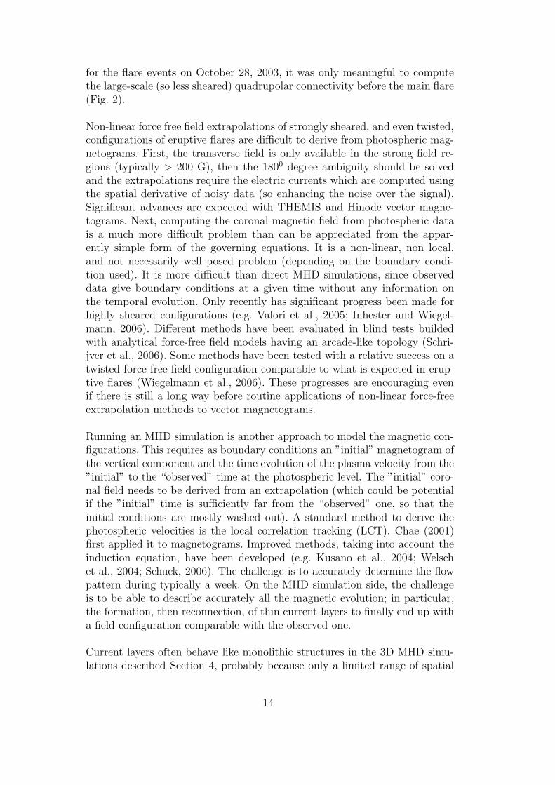
for the flare events on October 28, 2003, it was only meaningful to computethe large-scale (so less sheared) quadrupolar connectivity before the main flare(Fig. 2).

Non-linear force free field extrapolations of strongly sheared, and even twisted,configurations of eruptive flares are difficult to derive from photospheric mag-netograms. First, the transverse field is only available in the strong field re-gions (typically > 200 G), then the 1800 degree ambiguity should be solvedand the extrapolations require the electric currents which are computed usingthe spatial derivative of noisy data (so enhancing the noise over the signal).Significant advances are expected with THEMIS and Hinode vector magne-tograms. Next, computing the coronal magnetic field from photospheric datais a much more difficult problem than can be appreciated from the appar-ently simple form of the governing equations. It is a non-linear, non local,and not necessarily well posed problem (depending on the boundary condi-tion used). It is more difficult than direct MHD simulations, since observeddata give boundary conditions at a given time without any information onthe temporal evolution. Only recently has significant progress been made forhighly sheared configurations (e.g. Valori et al., 2005; Inhester and Wiegel-mann, 2006). Different methods have been evaluated in blind tests buildedwith analytical force-free field models having an arcade-like topology (Schri-jver et al., 2006). Some methods have been tested with a relative success on atwisted force-free field configuration comparable to what is expected in erup-tive flares (Wiegelmann et al., 2006). These progresses are encouraging evenif there is still a long way before routine applications of non-linear force-freeextrapolation methods to vector magnetograms.

Running an MHD simulation is another approach to model the magnetic con-figurations. This requires as boundary conditions an ”initial” magnetogram ofthe vertical component and the time evolution of the plasma velocity from the”initial” to the “observed” time at the photospheric level. The ”initial” coro-nal field needs to be derived from an extrapolation (which could be potentialif the ”initial” time is sufficiently far from the “observed” one, so that theinitial conditions are mostly washed out). A standard method to derive thephotospheric velocities is the local correlation tracking (LCT). Chae (2001)first applied it to magnetograms. Improved methods, taking into account theinduction equation, have been developed (e.g. Kusano et al., 2004; Welschet al., 2004; Schuck, 2006). The challenge is to accurately determine the flowpattern during typically a week. On the MHD simulation side, the challengeis to be able to describe accurately all the magnetic evolution; in particular,the formation, then reconnection, of thin current layers to finally end up witha field configuration comparable with the observed one.

Current layers often behave like monolithic structures in the 3D MHD simu-lations described Section 4, probably because only a limited range of spatial

14

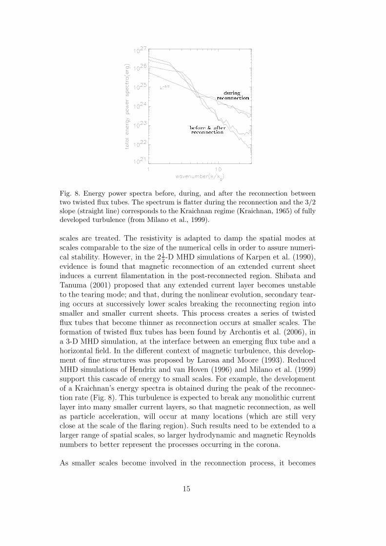
duringreconnectionbefore & afterreconnectionFig. 8. Energy power spectra before, during, and after the reconnection betweentwo twisted flux tubes. The spectrum is flatter during the reconnection and the 3/2slope (straight line) corresponds to the Kraichnan regime (Kraichnan, 1965) of fullydeveloped turbulence (from Milano et al., 1999).

scales are treated. The resistivity is adapted to damp the spatial modes atscales comparable to the size of the numerical cells in order to assure numeri-cal stability. However, in the 21

2-D MHD simulations of Karpen et al. (1990),

evidence is found that magnetic reconnection of an extended current sheetinduces a current filamentation in the post-reconnected region. Shibata andTanuma (2001) proposed that any extended current layer becomes unstableto the tearing mode; and that, during the nonlinear evolution, secondary tear-ing occurs at successively lower scales breaking the reconnecting region intosmaller and smaller current sheets. This process creates a series of twistedflux tubes that become thinner as reconnection occurs at smaller scales. Theformation of twisted flux tubes has been found by Archontis et al. (2006), ina 3-D MHD simulation, at the interface between an emerging flux tube and ahorizontal field. In the different context of magnetic turbulence, this develop-ment of fine structures was proposed by Larosa and Moore (1993). ReducedMHD simulations of Hendrix and van Hoven (1996) and Milano et al. (1999)support this cascade of energy to small scales. For example, the developmentof a Kraichnan’s energy spectra is obtained during the peak of the reconnec-tion rate (Fig. 8). This turbulence is expected to break any monolithic currentlayer into many smaller current layers, so that magnetic reconnection, as wellas particle acceleration, will occur at many locations (which are still veryclose at the scale of the flaring region). Such results need to be extended to alarger range of spatial scales, so larger hydrodynamic and magnetic Reynoldsnumbers to better represent the processes occurring in the corona.

As smaller scales become involved in the reconnection process, it becomes

15

necessary to consider a more complete set of physical equations. In particu-lar Ohm’s law needs to be better described than with a uniform resistivity. Inparticular the Hall term is expected to be significant (e.g. Ma and Bhattachar-jee, 2001; Morales et al., 2005). Moreover, microscopic plasma instabilities areexpected to develop, and these may lead to the development of an anomalousresistivity. Moreover, the electric fields generated exceed the Dreicer electricfield by several orders of magnitude. At this point, MHD will not be able todescribe the local processes involved in the reconnection of the thin layers, andkinetic theory is required (see e.g. the review of Heyvaerts, 2000). However,describing the full configuration by kinetic theory is not possible even withthe super-computers that will become available in the near future. The logicalstrategy is to use kinetic theory only in the thin volumes where MHD breaksdown, i.e. in the reconnecting current layers (Buchner, 2007). This approachis needed in order to link the global physics described by MHD (Section 4) tothe local acceleration of particles in multiple accelerating regions (e.g. Onofriet al., 2006; Turkmani et al., 2006; Dauphin et al., 2007).

MHD, and in particular magnetic extrapolations and the physics involved inQSLs, are needed to understand where electric current layers are forming; andthen, where reconnection is occurring. This approach is well adapted to un-derstand the temporal evolution of flares, as observed with imaging data (likeYohkoh, SOHO, THEMIS, TRACE, Hinode) since it allows us to localize thereconnection region within the global magnetic configuration. MHD simula-tions involving separatrices, and their generalization, QSLs, are expected tobe able, in the near future, to describe the evolution of flare ribbons; which inturn will provide a global view of the reconnection process in flares. However,MHD cannot describe the intimate physics of the reconnection processes, norparticle acceleration, since these processes need to be described by kinetic the-ory. Coupling these approaches is expected to give a global understanding ofthe flare/CME physics.

Acknowledgments: I thank G. Aulanier, C.H. Mandrini, and L. van Driel-Gesztelyi and the two referees for their help in improving the manuscript.

References

Aly, J. J., 1990. Do Current Sheets Necessarily Form in 3D Sheared MagneticForce-Free Fields ? In: The Dynamic Sun. p. 176.

Archontis, V., Galsgaard, K., Moreno-Insertis, F., Hood, A. W., 2006. Three-dimensional Plasmoid Evolution in the Solar Atmosphere. ApJ, 645, L161–L164.

Asai, A., Ishii, T. T., Kurokawa, H., Yokoyama, T., Shimojo, M., 2003. Evo-lution of Conjugate Footpoints inside Flare Ribbons during a Great Two-Ribbon Flare on 2001 April 10. ApJ, 586, 624–629.

16

Asai, A., Yokoyama, T., Shimojo, M., Masuda, S., Kurokawa, H., Shibata, K.,2004. Flare Ribbon Expansion and Energy Release Rate. ApJ, 611, 557–567.

Aulanier, G., DeLuca, E. E., Antiochos, S. K., McMullen, R. A., Golub, L.,2000. The Topology and Evolution of the Bastille Day Flare. ApJ, 540,1126–1142.

Aulanier, G., Demoulin, P., Schmieder, B., Fang, C., Tang, Y. H., 1998. Mag-netohydrostatic Model of a Bald-Patch Flare. Solar Physics, 183, 369–388.

Aulanier, G., Pariat, E., Demoulin, P., 2005. Current sheet formation in quasi-separatrix layers and hyperbolic flux tubes. A&A, 444, 961–976.

Aulanier, G., Pariat, E., Demoulin, P., Devore, C. R., 2006. Slip-RunningReconnection in Quasi-Separatrix Layers. Solar Physics, 238, 347–376.

Bagala, L. G., Mandrini, C. H., Rovira, M. G., Demoulin, P., 2000. Magneticreconnection: a common origin for flares and AR interconnecting arcs. A&A,363, 779–788.

Bogachev, S. A., Somov, B. V., Kosugi, T., Sakao, T., 2005. The Motions ofthe Hard X-Ray Sources in Solar Flares: Images and Statistics. ApJ, 630,561–572.

Buchner, J., 2006. Locating Current Sheets in the Solar Corona. Space ScienceReviews 122, 149–160.

Buchner, J., 2007. Simulation of the electric fields created by magnetic re-connection in the solar corona by combining large scale and plasma kineticapproaches. Advances in Space Research, submitted.

Chae, J., 2001. Observational Determination of the Rate of Magnetic HelicityTransport through the Solar Surface via the Horizontal Motion of Field LineFootpoints. ApJ, 560, L95–L98.

Dauphin, C., Vilmer, N., Anastasiadis, A., 2007. Particle acceleration andradiation in a flaring complex solar active regions modelled by cellular au-tomata. A&A, , submitted.

de Moortel, I., Galsgaard, K., 2006a. Numerical modelling of 3D reconnectiondue to rotational footpoint motions. A&A, 451, 1101–1115.

de Moortel, I., Galsgaard, K., 2006b. Numerical modelling of 3D reconnection.II. Comparison between rotational and spinning footpoint motions. A&A,459, 627–639.

Delannee, C., Aulanier, G., 1999. CME Associated with Transequatorial Loopsand a Bald Patch Flare. Solar Physics, 190, 107–129.

Demoulin, P., 2005. Magnetic Topologies: where Will Reconnection Occur ? In:Innes, D. E., Lagg, A., Solanki, S. A. (Eds.), ESA SP-596: Chromosphericand Coronal Magnetic Fields.

Demoulin, P., 2006. Extending the concept of separatrices to QSLs for mag-netic reconnection. Advances in Space Research 37, 1269–1282.

Demoulin, P., Bagala, L. G., Mandrini, C. H., Henoux, J. C., Rovira, M. G.,1997. Quasi-separatrix layers in solar flares. II. Observed magnetic configu-rations. A&A, 325, 305–317.

Demoulin, P., Henoux, J. C., Priest, E. R., Mandrini, C. H., 1996a. Quasi-Separatrix layers in solar flares. I. Method. A&A, 308, 643–655.

17

Demoulin, P., Mandrini, C. H., Rovira, M. G., Henoux, J. C., Machado, M. E.,1994. Interpretation of multiwavelength observations of November 5, 1980solar flares by the magnetic topology of AR 2766. Solar Physics, 150, 221–243.

Demoulin, P., Priest, E. R., Lonie, D. P., 1996b. Three-dimensional magneticreconnection without null points 2. Application to twisted flux tubes. JGR,101(A10), 7631–7646.

DeVore, C. R., Antiochos, S. K., Aulanier, G., 2005. Solar Prominence Inter-actions. ApJ, 629, 1122–1134.

Fletcher, L., Hudson, H. S., 2002. Spectral and Spatial Variations of FlareHard X-ray Footpoints. Solar Physics, 210, 307–321.

Fletcher, L., Lopez Fuentes, M. C., Mandrini, C. H., Schmieder, B., Demoulin,P., Mason, H. E., Young, P. R., Nitta, N., 2001a. A Relationship BetweenTransition Region Brightenings, Abundances, and Magnetic Topology. SolarPhysics, 203, 255–287.

Fletcher, L., Metcalf, T. R., Alexander, D., Brown, D. S., Ryder, L. A., 2001b.Evidence for the Flare Trigger Site and Three-Dimensional Reconnection inMultiwavelength Observations of a Solar Flare. ApJ, 554, 451–463.

Gaizauskas, V., Mandrini, C. H., Demoulin, P., Luoni, M. L., Rovira, M. G.,1998. Interactions between nested sunspots. II. A confined X1 flare in adelta-type sunspot. A&A, 332, 353–366.

Galsgaard, K., Titov, V. S., Neukirch, T., 2003. Magnetic Pinching of Hyper-bolic Flux Tubes. II. Dynamic Numerical Model. ApJ, 595, 506–516.

Gorbachev, V. S., Somov, B. V., 1988. Photospheric vortex flows as a causefor two-ribbon flares - A topological model. Solar Physics, 117, 77–88.

Grigis, P. C., Benz, A. O., 2005. The Evolution of Reconnection along anArcade of Magnetic Loops. ApJ, 625, L143–L146.

Hendrix, D. L., van Hoven, G., 1996. Magnetohydrodynamic Turbulence andImplications for Solar Coronal Heating. ApJ, 467, 887–893.

Hesse, M., Forbes, T. G., Birn, J., 2005. On the Relation between ReconnectedMagnetic Flux and Parallel Electric Fields in the Solar Corona. ApJ, 631,1227–1238.

Hesse, M., Schindler, K., 1988. A theoretical foundation of general magneticreconnection. JGR, 93(A12), 5559–5567.

Heyvaerts, J., 2000. Introduction to MHD. In: Rozelot, J. P., Klein, L., Vial,J.-C. (Eds.), LNP Vol. 553: Transport and Energy Conversion in the Helio-sphere. pp. 1–60.

Inhester, B., Wiegelmann, T., 2006. Nonlinear Force-Free Magnetic FieldExtrapolations: Comparison of the Grad Rubin and Wheatland SturrockRoumeliotis Algorithm. Solar Physics, 235, 201–221.

Karpen, J. T., Antiochos, S. K., Devore, C. R., 1990. On the formation ofcurrent sheets in the solar corona. ApJ, 356, L67–L70.

Kraichnan, R. H., 1965. Inertial-Range Spectrum of Hydromagnetic Turbu-lence. Physics of fluid 8, 1385–1387.

Krucker, S., Hurford, G. J., Lin, R. P., 2003. Hard X-Ray Source Motions in

18

the 2002 July 23 Gamma-Ray Flare. ApJ, 595, L103–L106.Kusano, K., Maeshiro, T., Yokoyama, T., Sakurai, T., 2004. Study of Magnetic

Helicity in the Solar Corona. In: Sakurai, T., Sekii, T. (Eds.), ASP Conf. Ser.325: The Solar-B Mission and the Forefront of Solar Physics. pp. 175–184.

Larosa, T. N., Moore, R. L., 1993. A Mechanism for Bulk Energization inthe Impulsive Phase of Solar Flares: MHD Turbulent Cascade. ApJ, 418,912–918.

Lau, Y. T., 1993. Magnetic Nulls and Topology in a Class of Solar FlareModels. Solar Physics, 148, 301–324.

Lau, Y.-T., Finn, J. M., 1990. Three-dimensional kinematic reconnection inthe presence of field nulls and closed field lines. ApJ, 350, 672–691.

Longcope, D. W., 2005. Topological Methods for the Analysis of Solar Mag-netic Fields. Living Reviews in Solar Physics 2, 1–58.

Longcope, D. W., Cowley, S. C., 1996. Current sheet formation along three-dimensional magnetic separators. Physics of Plasmas 3, 2885–2897.

Longcope, D. W., Klapper, I., 2002. A General Theory of Connectivity andCurrent Sheets in Coronal Magnetic Fields Anchored to Discrete Sources.ApJ, 579, 468–481.

Longcope, D. W., McKenzie, D., Cirtain, J., Scott , J., 2005. Observations ofSeparator Reconnection to an Emerging Active Region. ApJ, 630, 596–614.

Longcope, D. W., Silva, A. V. R., 1998. A current ribbon model for energystorage and release with application to the flare of 7 January 1992. SolarPhysics, 179, 349–377.

Longcope, D. W., Strauss, H. R., 1994. The form of ideal current layers inline-tied magnetic fields. ApJ, 437, 851–859.

Low, B. C., Wolfson, R., 1988. Spontaneous formation of electric current sheetsand the origin of solar flares. ApJ, 324, 574–581.

Ma, Z. W., Bhattacharjee, A., 2001. Hall magnetohydrodynamic reconnection:The Geospace Environment Modeling challenge. JGR, 106, 3773–3782.

Mandrini, C. H., Demoulin, P., Bagala, L. G., van Driel-Gesztelyi, L., Henoux,J. C., Schmieder, B., Rovira, M. G., 1997. Evidence of Magnetic Reconnec-tion from Hα, Soft X-Ray and Photospheric Magnetic Field Observations.Solar Physics, 174, 229–240.

Mandrini, C. H., Demoulin, P., Schmieder, B., Deluca, E. E., Pariat, E., Uddin,W., 2006. Companion Event and Precursor of the X17 Flare on 28 October2003. Solar Physics, 238, 293–312.

Mandrini, C. H., Demoulin, P., Schmieder, B., Deng, Y. Y., Rudawy, P., 2002.The role of magnetic bald patches in surges and arch filament systems. A&A,391, 317–329.

Mandrini, C. H., Rovira, M. G., Demoulin, P., Henoux, J. C., Machado, M. E.,Wilkinson, L. K., 1993. Evidence for magnetic reconnection in large-scalemagnetic structures in solar flares. A&A, 272, 609–620.

Martin, S. F., Harvey, K. H., 1979. Ephemeral active regions during solarminimum. Solar Physics, 64, 93–108.

Milano, L. J., Dmitruk, P., Mandrini, C. H., Gomez, D. O., Demoulin, P.,

19

1999. Quasi-Separatrix Layers in a Reduced Magnetohydrodynamic Modelof a Coronal Loop. ApJ, 521, 889–897.

Molodenskii, M. M., Syrovatskii, S. I., 1977. Magnetic fields of active regionsand their zero points. Soviet Astronomy 21, 734–741.

Moore, R. L., Larosa, T. N., Orwig, L. E., 1995. The wall of reconnection-driven magnetohydrodynamic turbulence in a large solar flare. ApJ, 438,985–966.

Morales, L. F., Dasso, S., Gomez, D. O., 2005. Hall effect in incompressiblemagnetic reconnection. JGR, 110, 4204.

Onofri, M., Isliker, H., Vlahos, L., 2006. Stochastic Acceleration in TurbulentElectric Fields Generated by 3D Reconnection. Physical Review Letters96 (15), 151102–151105.

Pariat, E., Aulanier, G., Schmieder, B., Georgoulis, M. K., Rust, D. M.,Bernasconi, P. N., 2004. Resistive Emergence of Undulatory Flux Tubes.ApJ, 614, 1099–1112.

Pevtsov, A. A., Canfield, R. C., Zirin, H., 1996. Reconnection and Helicity ina Solar Flare. ApJ, 473, 533–538.

Pontin, D. I., Galsgaard, K., Hornig, G., Priest, E. R., 2005. A fully magne-tohydrodynamic simulation of 3D non-null reconnection. Phys. Plasmas 12,052307–10.

Priest, E., Forbes, T., 2000. Magnetic reconnection : MHD theory and appli-cations. Cambridge University Press, Cambridge, UK.

Priest, E. R., Demoulin, P., 1995. Three-dimensional magnetic reconnectionwithout null points. 1. Basic theory of magnetic flipping. JGR, 100(A9),23443–23464.

Priest, E. R., Forbes, T. G., 1992. Magnetic flipping - Reconnection in threedimensions without null points. JGR, 97, 1521–1531.

Priest, E. R., Hornig, G., Pontin, D. I., 2003. On the nature of three-dimensional magnetic reconnection. JGR, 108(A7), 1285.

Schindler, K., Hesse, M., Birn, J., 1988. General magnetic reconnection, par-allel electric fields, and helicity. JGR, 93(A12), 5547–5557.

Schrijver, C. J., Derosa, M. L., Metcalf, T. R., Liu, Y., McTiernan, J., Regnier,S., Valori, G., Wheatland, M. S., Wiegelmann, T., 2006. Nonlinear Force-Free Modeling of Coronal Magnetic Fields Part I: A Quantitative Compar-ison of Methods. Solar Physics, 235, 161–190.

Schuck, P. W., 2006. Tracking Magnetic Footpoints with the Magnetic Induc-tion Equation. ApJ, 646, 1358–1391.

Shibata, K., Tanuma, S., 2001. Plasmoid-induced-reconnection and fractal re-connection. Earth, Planets, and Space 53, 473–482.

Su, Y. N., Golub, L., van Ballegooijen, A. A., gros, M., 2006. Analysis ofMagnetic Shear in an X17 Solar Flare on October 28, 2003. Solar Physics,236, 325–349.

Svestka, Z., Cliver, E. W., 1992. History and Basic Characteristics of EruptiveFlares. In: Svestka, Z., Jackson, B. V., Machado, M. E. (Eds.), LNP Vol.399: IAU Colloq. 133: Eruptive Solar Flares. pp. 1–11.

20

Titov, V. S., 2005. Pinching of coronal fields. In: Reconnection of MagneticFields (eds. J. Birn and E.R. Priest). Cambridge University Press, Cam-bridge, UK, p. 5.3.

Titov, V. S., Galsgaard, K., Neukirch, T., 2003. Magnetic Pinching of Hyper-bolic Flux Tubes. I. Basic Estimations. ApJ, 582, 1172–1189.

Titov, V. S., Hornig, G., Demoulin, P., 2002. Theory of magnetic connectivityin the solar corona. JGR, 107(A8), 1164.

Titov, V. S., Priest, E. R., Demoulin, P., 1993. Conditions for the appearanceof ”bald patches” at the solar surface. A&A, 276, 564–570.

Turkmani, R., Cargill, P. J., Galsgaard, K., Vlahos, L., Isliker, H., 2006. Par-ticle acceleration in stochastic current sheets in stressed coronal active re-gions. A&A, 449, 749–757.

Valori, G., Kliem, B., Keppens, R., 2005. Extrapolation of a nonlinear force-free field containing a highly twisted magnetic loop. A&A, 433, 335–347.

Welsch, B. T., Fisher, G. H., Abbett, W. P., Regnier, S., 2004. ILCT: Recov-ering Photospheric Velocities from Magnetograms by Combining the Induc-tion Equation with Local Correlation Tracking. ApJ, 610, 1148–1156.

Wiegelmann, T., Inhester, B., Kliem, B., Valori, G., Neukirch, T., 2006.Testing non-linear force-free coronal magnetic field extrapolations with theTitov-Demoulin equilibrium. A&A, 453, 737–741.

Williams, D. R., Torok, T., Demoulin, P., van Driel-Gesztelyi, L., Kliem, B.,2005. Eruption of a Kink-unstable Filament in NOAA Active Region 10696.ApJ, 628, L163–L166.

Yokoyama, T., Shibata, K., 1994. What is the condition for fast magneticreconnection? ApJ, 436, L197–L200.

Zwingmann, W., Schindler, K., Birn, J., 1985. On sheared magnetic field struc-tures containing neutral points. Solar Physics, 99, 133–143.

21