LUND UNIVERSITY

PO Box 117221 00 Lund+46 46-222 00 00

When errors become the rule

A survey of transformation-based learningUneson, Marcus

2011

Link to publication

Citation for published version (APA):Uneson, M. (2011). When errors become the rule: A survey of transformation-based learning. ComputerScience, Lund University.

General rightsCopyright and moral rights for the publications made accessible in the public portal are retained by the authorsand/or other copyright owners and it is a condition of accessing publications that users recognise and abide by thelegal requirements associated with these rights.

• Users may download and print one copy of any publication from the public portal for the purpose of private studyor research. • You may not further distribute the material or use it for any profit-making activity or commercial gain • You may freely distribute the URL identifying the publication in the public portalTake down policyIf you believe that this document breaches copyright please contact us providing details, and we will removeaccess to the work immediately and investigate your claim.

When Errors Become the RuleA Survey of Transformation-Based Learning

Marcus Uneson

esis for a diploma in computer science, 30 ECTS credits,Department of Computer Science, Faculty of Science, Lund University

Examensarbete för 30hp,Institutionen för datavetenskap, Naturvetenskapliga fakulteten, Lunds universitet

When Errors Become the Rule:A Survey of Transformation-Based LearningAbstractTransformation-based learning (TBL) is a maine learning method for sequential classification,invented by Eric Brill (Brill, 1993c, 1995a). It is widely used within natural language processing(but surprisingly lile in other areas).TBL is a simple yet flexible paradigm, whi aieves competitive or even state-of-the-art per-

formance in several areas and does not overtrain easily. It is especially successful at cating local,fixed-distance dependencies. e learned representation – an ordered list of transformation rules– is compact and efficient, with clear, declarative semantics. Individual rules are interpretableand oen meaningful to humans.e present thesis has two main parts. First and foremost, we offer a survey of the most impor-

tant theoretical work on TBL. It is intended to be informal but relatively comprehensive, address-ing a perceived gap in the literature. Second, in a more practical part, we describe a recursive,parallelizable rephrasing, well suited for declarative languages, of a fast imperative learning al-gorithm proposed by Ngai and Florian (2001b). We implement and test this algorithm in thefunctional language Haskell.

När fel blir regel:En översikt över transformationsbaserad inlärningSammanfattningTransformationsbaserad inlärning (Transformation-based learning, TBL) är en maskininlärnings-metod för sekventiell klassificering, uppfunnen av Eric Brill (Brill, 1993c, 1995a). Den användsregelmässigt för många uppgier inom automatisk processning av naturligt språk (men förvå-nansvärt sällan på andra områden).TBL är en enkel men flexibel metod som når konkurrenskraiga resultat på många områden,

utan a vara sårbar för överträning. Den kan särskilt framgångsrikt fånga lokala beroenden in-om sekvensintervall av förbestämd storlek. Den representation som lärs in – en ordnad lista avtransformationsregler – är kompakt o effektiv, med deklarativ semantik. Enskilda regler är tolk-ningsbara o oa meningsbärande för människor.Föreliggande uppsats har två huvuddelar. I den första ger vi en översikt av de viktigaste teore-

tiska arbetena rörande TBL. Översikten är informellt hållen men förhållandevis omfaande; denavses därmed fylla en lua i den befintliga lieraturen.I den andra delen, mer praktiskt inriktad, beskriver vi en rekursiv, parallelliserbar formulering,

väl lämpad för deklarativa programspråk, av en effektiv imperativ algoritm för inlärningsfasen,föreslagen av Ngai and Florian (2001b). Vi implementerar o testar denna algoritm i det funktio-nella programmeringsspråket Haskell.

2

Prefacee present work provides a survey of Transformation-Based Learning (TBL), a supervised ma-ine learning algorithm for sequential classification invented by Eric Brill (Brill, 1993a, 1995a).It also presents an efficient training algorithm for TBL in a declarative paradigm. In our view,both TBL and declarative programming deserve wider aention. On the whole, the work pre-sented here concentrates on the former, but declarativity resurfaces also in our discussion of howa well-designed domain-specific language may extend the expressivity and usefulness of TBL.is is a thesis in Computer Science, rather than, say, Computational Linguistics. It is intended

to be readable without mu acquaintance with neither specialized linguistic terminology nor thetoolbox of computational linguistics. Linguistic terminology cannot be entirely avoided, however,and some familiarity with the concepts and methods will certainly do no harm. To date, TBL hasbeen applied almost exclusively to natural language data, and most citations must necessarilybe drawn from that area. Where deemed necessary, we have tried to explain non-elementaryconcepts in a phrase or two in the body text; sometimes we also provide more extensive but lesscrucial comments in endnotes. is is hopefully enough to illustrate the inputs and outputs of acertain problem, but it is almost certainly not enough to convey the rationales behind posing it inthe first place. Furthermore, in some cases, where exact understanding of the terminology mightnot be needed for the understanding of the algorithmic aspects, we found that further detoursadded more cluer than clarity. When explanations given here are insufficient, we refer to somededicated textbook in Computational Linguistics, for instance the excellent Jurafsky and Martin(2008). Similarly, for maine learning terminology, we refer to Mitell (1997) (whi, however,has lile to say specifically about classification of sequences).is thesis began life as a apter of a yet-to-be-finished PhD thesis; but later it ran away, got

a life of its own and did not want to fit in (apparently this may happen to ildren of the brainas well as ildren of the flesh). I’d like to thank Torbjörn Lager for valuable encouragementand feedba on short notice, Mats-Eeg Olofsson for meticulous proofreading, Radu Florian forgraciously providing tex sources of the FnTBL algorithm, and Karin Palm-Lindén for generoushospitality in critical moments.

3

Contents

1 Introduction 61.1 Four aspects of a restaurant conversation . . . . . . . . . . . . . . . . . . . . . . 61.2 Classification of elements and sequences . . . . . . . . . . . . . . . . . . . . . . 71.3 e present work: Classification by transformation . . . . . . . . . . . . . . . . 9

2 Plain vanilla TBL 112.1 A painting analogy . . . . . . . . . . . . . . . . . . . . . . . . . . . . . . . . . . 112.2 Algorithmic overview . . . . . . . . . . . . . . . . . . . . . . . . . . . . . . . . 122.3 Free with vanilla: TBL strong points . . . . . . . . . . . . . . . . . . . . . . . . 212.4 TBL vs. Decision Trees . . . . . . . . . . . . . . . . . . . . . . . . . . . . . . . 262.5 TBL in practice . . . . . . . . . . . . . . . . . . . . . . . . . . . . . . . . . . . . 27

3 Adding flavour 323.1 Extending the hypothesis domain . . . . . . . . . . . . . . . . . . . . . . . . . . 323.2 Extending the hypothesis range . . . . . . . . . . . . . . . . . . . . . . . . . . . 363.3 Improving efficiency . . . . . . . . . . . . . . . . . . . . . . . . . . . . . . . . . 393.4 Widening the bolene: Unsupervised learning . . . . . . . . . . . . . . . . . 423.5 Abstracting the problem: Template compositionality and DSLs . . . . . . . . . . 43

4 Fast, declarative TBL 474.1 Notation . . . . . . . . . . . . . . . . . . . . . . . . . . . . . . . . . . . . . . . 484.2 Algorithmic overview . . . . . . . . . . . . . . . . . . . . . . . . . . . . . . . . 484.3 A low-level view: Updating GB . . . . . . . . . . . . . . . . . . . . . . . . . . 504.4 A high-level view: Computing GB∆ . . . . . . . . . . . . . . . . . . . . . . . . 504.5 Implementation notes . . . . . . . . . . . . . . . . . . . . . . . . . . . . . . . . 534.6 Algorithm time and memory consumption . . . . . . . . . . . . . . . . . . . . . 55

5 Conclusion and future directions 57

References 61

4

List of Figures1 A barnyard scene . . . . . . . . . . . . . . . . . . . . . . . . . . . . . . . . . . . 112 Data flow of TBL training, Brill’s original algorithm . . . . . . . . . . . . . . . . 133 Learning curve in the presence of relevant and irrelevant templates . . . . . . . 254 NP unks with encodings . . . . . . . . . . . . . . . . . . . . . . . . . . . . . . 295 Parse trees with encodings . . . . . . . . . . . . . . . . . . . . . . . . . . . . . . 306 Template extraction from decision tree . . . . . . . . . . . . . . . . . . . . . . . 347 Bit string encoding of TBL rule learning . . . . . . . . . . . . . . . . . . . . . . 358 Applying a Transformation-Based Regression rule . . . . . . . . . . . . . . . . . 389 Chunking Portuguese . . . . . . . . . . . . . . . . . . . . . . . . . . . . . . . . 4310 Dialogue act tagging in μ-TBL . . . . . . . . . . . . . . . . . . . . . . . . . . . . 4511 DSL templates for Portuguese unking . . . . . . . . . . . . . . . . . . . . . . 4612 Data flow of TBL training, extended with state . . . . . . . . . . . . . . . . . . 4713 Vicinity of a node . . . . . . . . . . . . . . . . . . . . . . . . . . . . . . . . . . 4914 e FnTBL algorithm (Ngai and Florian, 2001b). . . . . . . . . . . . . . . . . . . 5115 Partitioning a corpus with respect to a rule and a template set . . . . . . . . . . 5216 Fast, declarative TBL in functional-style pseudocode . . . . . . . . . . . . . . . 5417 Fast, declarative TBL: Algorithm performance . . . . . . . . . . . . . . . . . . . 5618 Fast, declarative TBL: Memory usage . . . . . . . . . . . . . . . . . . . . . . . . 56

List of Tables1 POS tagging templates . . . . . . . . . . . . . . . . . . . . . . . . . . . . . . . . 142 Trace of minimal TBL learning session . . . . . . . . . . . . . . . . . . . . . . . 163 Trace of minimal TBL application session . . . . . . . . . . . . . . . . . . . . . 164 POS tagging templates, generalized . . . . . . . . . . . . . . . . . . . . . . . . . 175 Handling templates with out-of-bound accesses . . . . . . . . . . . . . . . . . . 186 POS tagging transformations, English . . . . . . . . . . . . . . . . . . . . . . . 237 Stress and word accent prediction, Swedish . . . . . . . . . . . . . . . . . . . . 238 Sample TBL applications . . . . . . . . . . . . . . . . . . . . . . . . . . . . . . . 28

5

1 INTRODUCTION

1 Introduction1.1 Four aspects of a restaurant conversationConsider the following hypothetical fragment of a dialogue, perhaps between a head waiter anda nervous, newly employed colleague in an overworked restaurant kiten.

– Replace the fork on table four.– OK. Should I apologize for the wait?– For now it’s enough to light the candle on the table.

It is a perfectly ordinary piece of language, English, in this particular case – indeed, it maybe ordinary enough to be uninteresting to most people. But let us assume that we have somevalid reason to study this sample – maybe we are engineers and want to build some tenicalapplicationwhimight receive it as input, or maybewe are linguists andwould like to investigatethe language phenomena it exemplifies.In any case, we probably have many more samples like it. We would like to describe them all in

some abstracted way, whi highlights their similarities and differences with regard to the aspectwe currently happen to be interested in. For instance, in Example 1 our domain of interest is thesequence of words, and to ea element of this sequence we wish to assign a part-of-spee, orPOS – classes su as verb, noun, preposition, etc. We will use the notation w1/1 w2/2 . . .to indicate su a classification (and generalize as needed).i ¹

(1) – Replace/ the/ fork/ on/ table/ four/ ./.– OK/ ./. Should/ I/ apologize/ for/ the/ wait/ ?/.– For/ now/ it/ ’s/ enough/ to/ light/ the/ candle/on/ the/ table/ ./.

In another scenario (Example 2), we are more interested in the turns of the dialogue itself thanin the exact wordings of the uerances. In dialogue act tagging, we try to label entire uerancesby an abstracted representation of the speaker’s intentions: , , , , , . . .

(2) – Replace the fork on table four./– OK./Should I apologize for the wait?/

– For now it’s enough/to light the candle on the table./

Going from larger elements to very small ones, in Example 3 we instead want to study howleers correspond to spee sounds (or, with a posh term, their graphophonemic relationships).Here, the data consists of an alignment of ea leer to its corresponding pronunciation (boomrow, in IPA²), with “_” as a placeholder when one-to-one-alignment is inappropriate. Similar

¹Roman numbers refer to the notes at the end of the paper, mostly elaborating on specifically linguistic issues – here,for instance, the cryptic , , etc.

²IPA is the International Phonetic Alphabet, http://www.langsci.ucl.ac.uk/ipa/ipachart.html.

6

1.2 Classification of elements and sequences 1 INTRODUCTION

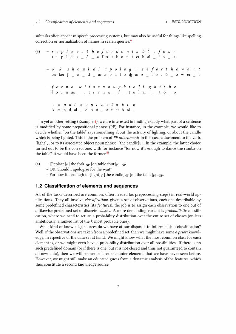
subtasks oen appear in spee processing systems, but may also be useful for things like spellingcorrection or normalization of names in sear queries.ii

(3) – rɹ

ei

pp

llaeɪ

cs

e_

tð

h_

eə

ff

oɔ

rɹ

kk

oɑ

nn

ttaeɪ

bb

ləl

e_

ff

oɔ

u_

rɹ

– ooʊ

kkeɪ

sʃ

h_

oʊ

u_

ld

d_

Iaɪ

aə

pp

oa

lloə

gʤ

iaɪ

zz

e_

ff

oɔ

rɹ

tð

h_

eə

ww

aeɪ

i_

tt

– ff

oɔ

rɹ

nn

oaʊ

w_

iɪttss

eɪ

nn

oʌ

u_

gf

h_

ttou

lliaɪ

g_

h_

tttð

h_

eə

ck

aæ

nn

dd

ləl

e_

oɑ

nn

tð

h_

eə

ttaeɪ

bb

ləl

e_

In yet another seing (Example 4), we are interested in finding exactly what part of a sentenceis modified by some prepositional phrase (PP). For instance, in the example, we would like todecide whether “on the table” says something about the activity of lighting, or about the candlewhi is being lighted. is is the problem of PP aament : in this case, aament to the verb,[light]V, or to its associated object noun phrase, [the candle]NP. In the example, the laer oiceturned out to be the correct one; with for instance “for now it’s enough to dance the rumba onthe table”, it would have been the former.iii

(4) – [Replace]V [the fork]NP [on table four]PP−NP.– OK. Should I apologize for the wait?– For now it’s enough to [light]V [the candle]NP [on the table]PP−NP.

1.2 Classification of elements and sequencesAll of the tasks described are common, oen needed (as preprocessing steps) in real-world ap-plications. ey all involve classification: given a set of observations, ea one describable bysome predefined aracteristics (its features), the job is to assign ea observation to one out ofa likewise predefined set of discrete classes. A more demanding variant is probabilistic classifi-cation, where we need to return a probability distribution over the entire set of classes (or, lessambitiously, a ranked list of the k most probable ones).What kind of knowledge sources do we have at our disposal, to inform su a classification?

Well, if the observations are taken from a predefined set, then wemight have some a priori knowl-edge, irrespective of the data set at hand. We might know what the most common class for eaelement is, or we might even have a probability distribution over all possibilities. If there is nosu predefined domain (or if there is one, but it is not closed and thus not guaranteed to containall new data), then we will sooner or later encounter elements that we have never seen before.However, we might still make an educated guess from a dynamic analysis of the features, whithus constitute a second knowledge source.

7

1.2 Classification of elements and sequences 1 INTRODUCTION

Actually, in Examples 1 – 3, what we are given is not a set of observations, but a set of sequencesof observations. e classification of ea element depends on its local context: its neighbours(within some not-too-wide window), and their classifications. Sequential classification tasks oenappear when we deal with symbols ordered in time or space, su as those present in humanlanguage. In su tasks, an additional, third knowledge source – by definition – is the sequentialcontext: whi are the neighbours of the sample we are trying to classify, what are their features,and what is our (current) idea of their classification?e example applications illustrate the varying importance of these knowledge sources:

• In part-of-spee tagging, the domain is semi-closed: most words are likely to be knownbeforehand, and we might well have them specified in a lexicon. Still, previously unseenwords are certain to occur now and then in any real-world application, and we are muhelped by being able to make intelligent guesses from dynamic feature analysis – for in-stance, guessing that staycation is a noun and defriend is a verb.³ Generally, ambiguouswords cannot be resolved without sequential context.

• In dialogue act tagging the domain is truly infinite, and only seldom will we listen to ut-terances whi we have heard in their entirety before (when it does happen, it is usuallyshort phrases: single words, or word-like groups of words: yes, what’s up, I don’t know).us, appropriate feature extraction is crucial. Sequential context is clearly important – theanswer to a is mu more likely to be an instance of or than , nomaer the phrasing.

• In finding leer-to-sound correspondences, we are very unlikely to encounter any previ-ously unseen leers, us, feature extraction is pointless – whatever we might wish to usefeatures for would beer have been included elsewhere, as a priori knowledge. e ba-ground knowledge specifies default correspondences and sequential context can (crucially,for many languages) be used to emend these.

• In PP aament, the domain is again infinite, but in contrast to the other examples, se-quential context has no influence: the fact that a PP was aaed to the verb in the previoussentence tells us nothing about the current one. us, intelligent feature extraction is thesingle source of information.

Another interesting dimension along whi these examples vary is the well-definedness of theclassifier range. In PP aament, we generally have two answers tooose from, and if we look ata wide enough context, exactly one of them is correct. In finding leer-to-sound correspondences,we may argue about the best alignment, but there is usually reasonable agreement on the lexicalpronunciation (at least if we consider some reference variety of the target language). POS taggingis triier: it is only meaningful with respect to some stipulatively defined tagset, specific to alanguage and sometimes also to a certain data set.⁴ Dialogue act tagging, finally, is less studied and

³New entries in the Oxford English Dictionary 2010.⁴Of course, su tagsets are not created in a vacuum; they build on ea other and for a given language, differencesbetween them partly reflect the number of subdivisions made. us, a larger set can oen be converted to a smallerwith relative ease.

8

1.3 e present work: Classification by transformation 1 INTRODUCTION

understood; thus, it has the aracteristics of POS tagging to an even higher extent, with tagsetsdepending also on domain or seing. As can be expected, human interannotator agreement forthe four tasks decreases in the order given.

1.3 The present work: Classification by transformatione sequences we have encountered so far are all finite and not very long. On the other hand, wemay have many of them – thousands, millions, or billions – and we certainly want a computer tohelp us. One road to automate the ore is to implement a classifier as a set of manually specifiedrules. For some combinations of task and data, this is actually the best solution. Restricting thedata type to natural language for the sake of discussion, it is easy enough to write a leer-to-sound converter for Finnish, Spanish, or Turkish by enumerating the few necessary rules in apage or two. Mu more substantial human effort was invested into the thousands of rules of theEngCG POS tagger (Karlsson et al., 1995), for a long time one of the best part-of-spee taggersfor English.⁵For most instances of sequential classification, including those illustrated in Section 1.1, this

approa is simply infeasible: there are too many and too weak dependencies, and it is far too la-borious to try to specify them by hand. Instead, we may oose among many reasonable mainelearning approaes: decision trees, hidden Markov models, neural networks, maximum entropymodels, memory-based learning, to mention just a few. ese are well-known teniques in themaine learning community, and certainly good oices in many situations. eir main draw-ba for the tasks we are interested in is the opacity of the learned representation. For the men-tioned teniques, learning amounts to filling a bla, inscrutable box with estimated parameters.e exception is decision trees, whi do slightly beer: they give us a somewhat interpretabletree with if...else questions at every node. ese, however, tend to be overwhelmingly manyfor any real-world task.e focus of the present thesis is on yet another maine learning method: Transformation-

based learning (TBL). It was invented by Eric Brill (Brill, 1993c, 1995a) and has been refined by himand many others since. In terms of the teniques mentioned, TBL is a hybrid: its representationinvolves rules, or transformations, but these are learned automatically from the training data.Rules are iteratively created and evaluated based on how well they deal with the current set oferrors in the data; hence, the approa is oen termed error-driven.TBL is typically used as a supervised maine learning tenique for classification of sequences,

where ea element is represented as a symbolic feature vector and assigned a single symbolicvalue in the classification. Interpretability of representation is but one out of several propertieswhi make the method appetizing for applications involving natural language; some others arethe natural ease with whi it handles local (especially fixed-width) dependencies; its resistanceto overtraining; and its general flexibility and adaptability to different tasks. In the next section,we will look further into these. e method itself, however, does not (and good implementationsshould not) make any assumptions whi are valid only for natural language classification tasks.To be sure, natural language abounds with ambiguities to pit maine learning methods against,TBL or others; and it also abounds with weak, mostly local, and incompletely understood depen-

⁵EngCG later got augmented by automatically derived rules. See also Section 3.2.2.

9

1.3 e present work: Classification by transformation 1 INTRODUCTION

dencies whi these methods may exploit. But Life offers many examples of symbols ordered intime or space – just to mention a few, DNA and protein sequences, musical notes, suns and cloudsin weather forecasts.Furthermore, the problem aracteristics described are typical, not mandatory – with the ap-

propriate problem encoding, it is perfectly possible to apply TBL to most any classification task. Inaddition, many extensions have been suggested, some of whi are specifically aimed at wideningthe method’s expressive power. For instance, TBL can be rebuilt into a regressor (with real-valuedoutput), or a probabilistic classifier (with a probability distribution over the entire set of classesas output); see further Section 3.ere are two immediate aims to the present thesis. e first and most important one is theoret-

ical: to provide a self-contained but still relatively comprehensive introduction to an interestingmaine learning tenique, without mu formal detail and reasonably readable also withoutlinguistic training. us, we give an overview of vanilla TBL as per Brill (1993c, 1995a), and abrief survey of the most important later developments.⁶e second aim is practical: to propose, implement, and test a declarative and parallelizable

phrasing of a fast algorithm for learning TBL.In a slightly broader sense, however, this thesis hopes to promote TBL as a general maine

learning method, useful for many kinds of linguistic tasks but potentially also for other typesof supervised sequential classification problems. For some reason, despite its many strong pointsand several successful use cases, many Computational Linguists still associate TBLwith the ratherrestricted task of part-of-spee tagging. More significantly, outside that relatively small commu-nity, TBL is practically unheard of (cf. Table 8). In our view, TBL could well be tried on a widerarray of problems, posed by Computational Linguists or others.is thesis is organized as follows. Section 2 and Section 3, together making up the main part

of the work, provide a survey of original TBL and later improvements. In Section 2, we reviewthe original algorithm proposed by Brill (1993c, 1995a), its inherent strong points, and the rela-tion to its distant cousin decision trees. is section also contains a brief overview of TBL usesin practical applications – many and varied, but, as mentioned, almost exclusively within therealm of Computational Linguistics and its closest neighbours. Section 3 provides an overview ofthe most important developments whi have appeared later, aimed at augmenting the originalparadigm in different directions. We review aempts to extend the range of possible inputs andthe expressivity of the output; to relax the amount of supervision needed; to improve efficiency;and to ease the problem description.Section 4 exhibits the algorithmic content of the present work: a recursive phrasing of a fast

training algorithm, parallelizable and well suited for declarative languages. Section 5 concludesand hints at some possible future directions.

⁶A by-product of this work is a TBL bibliography, at the time of writing comprising around 180 entries. It is an updateand slight extension of a similarly scoped bibliography (with around 75 entries) collected up until 2002 by TorbjörnLager, http://www.ling.gu.se/~lager/Mutbl/bibliography.html; this is likely where the updated bibli-ography will end up as well.

10

2 PLAIN VANILLA TBL

Figure 1: A barnyard scene, for transformation-based painters. From Samuel (1998b)

2 Plain vanilla Transformation-Based Learning2.1 A painting analogyA useful TBL picture-painting analogy is offered by Samuel (1998b), who aributes it to TerryHarvey. It generates several of the right intuitions, so we will retell it here (slightly adapted).Consider the barnyard picture in Figure 1 (where colours have been named rather than rendered

for ease of exposition). A painter comes by. As it happens, he is actually a transformation-basedpainter, whi is mostly like any other painter, except he does not ever want to ange from asmaller brush to a larger. He is also more-than-average cavalier about making mistakes, claimingthat they can always be fixed later.Our painter finds the barnyard picture and decides to reproduce it on his own canvas, as follows.

First, he looks at the current state of his painting (a blank canvas) and compares it to the target,or truth, represented by the figure. He notes that the most efficient way to reduce the differencebetween his painting and the truth is to take the largest brush he has and paint the entire canvasblue. When the paint has dried, he again compares the current state of his painting to the truth.is time he finds that the easiest way to increase the similarity to the target is to take a slightlysmaller brush and paint the filled outlines of a red barn. ere is no need to worry about non-reddetails, su as windows, doors, and roof, as these will be taken care of in later stages, by smallerbrushes.And so our painter goes on. With ea ange of colour, he pis a finer brush and uses it with

increasingly thin and precise strokes. Coarser brushes, used early on, cover a large part of thepicture – they add a lot of paint, but they also make many mistakes. With later, thinner brushesless paint will be added, but also fewer errors. e final step might be to fill in the fine bla lineswith a very fine brush.e main point of the analogy is that the painter uses a sequence of colour-brush pairs, in de-

11

2.2 Algorithmic overview 2 PLAIN VANILLA TBL

scending order according to how mu paint they add to the canvas. Ea point of the canvasmay be repainted several times; although we can be convinced that the overall result looks in-creasingly like the target with ea application of a brush, we cannot be sure about the colour ofa specific point until all brushes have been applied.

2.2 Algorithmic overviewTransformation-based learning works in mu the same way as transformation-based painting.e method produces a sequence of rules, or transformations, ordered aer impact. Early rulesare very general and may ange classifications on large fractions of the data, usually commiingerrors in so doing. Subsequent rules are more specific andmay correct errors introduced by earlierones. A single transformation rule has the general form

if CONDITION(x) then do ACTION(x)

where x is a data sample; CONDITION, sometimes referred to as “context”, is a predicate⁷ onaributes of x and/or its local context; and ACTION anges some aribute of x. e rules areinduced automatically from the training data. e actual structure of CONDITION and ACTION isspecified by paerns known as templates; thus, templates define the transformation space.e main data structures and the data flow of TBL training (as presented in the seminal works

Brill (1993c) and Brill (1995a)) are shown in Figure 2.⁸ e output of the learning algorithm isan ordered sequence of transformation rules. New data (once it has been initialized in the sameway as the training data, see below) can now be classified by applying this sequence of learnedtransformations to it. In the following, we look at the data sets; at the templates, and at the flowof control. Finally, we return to some critical points where design oices lurk.

2.2.1 CorporaLike most maine learning methods, TBL takes as point of departure a data set of a certain size.For applications dealing with natural language, su a data set is usually referred as a corpus –indeed, corpora are the bread and buer of Computational Linguistics.⁹In the TBL case, this data set is assumed to come with reference classifications, making it a

reference corpus. us, TBL is a supervised method: it depends on the existence of some annota-tions whi can be taken as truth. e annotations are usually provided (or at least proof-read)by humans. Manually annotated corpora thus represent large investments, sometimes enormous,and creating them from scrat for a single project is rarely an option.

⁷A predicate is a boolean-valued function, i.e., it returns true or false.⁸Somewhat unconventionally, we avoid traditional pseudocode, focusing on flow of data rather than flow of control.is view fits beer with the declarative phrasing we will use later (Section 4). For more traditional descriptions,we refer to Brill (1995a) (or almost any other paper whi introduces the algorithm).

⁹A corpus, pl. corpora, is basically a sizable collection of real-world natural language data – text or spee or some-thing more exotic, like video recordings of sign language. We use that term because it is the most common for thetasks TBL has been applied to. However, it was not created by any transformation-based deities, and the readershould feel free to replace it with “big data set” at any time. For non-linguistic applications, this may roll moresmoothly off the tongue.

12

2.2 Algorithmic overview 2 PLAIN VANILLA TBL

Figure 2: Data flow of TBL training, Brill’s original algorithm. Main loop in heavier stroke.

A corpus can generally be thought of as a set of items whi are independent of ea other,by nature or by assumption, with respect to the task at hand. For instance, in POS tagging (Ex-ample 1), we can be reasonably sure that the POS of the words in the current sentence does notdepend on those in the previous one. In dialogue act tagging, ea uerance (Example 2) is clearlydependent on the previous one, but the dialogue acts in one conversation are likely independentof those in another. Partitioning the corpus into a set of subsets for whi we can assume mu-tual independence is highly beneficial, for the quality of the learned representation as well as theefficiency with whi it can be learned. To tag POS, we will want our corpus split into sentence-sized unks. For the case of dialogue acts, the corpus will hopefully contain some delimitersdistinguishing individual dialogues (this case also illustrates that the need of relevant and reliableannotations may go beyond individual samples). e individual classifications are oen calledtags (irrespective of their being true or not, and irrespective of the task at hand).¹⁰ In the TBLcase, we will oen speak of the training corpus, whi is essentially the reference corpus with theannotations deleted.

13

2.2 Algorithmic overview 2 PLAIN VANILLA TBL

Template Change A to B whenever …

pos:A>B <- pos:C@[-1] …the preceding word has pos Cpos:A>B <- pos:C@[2] …the word two aer has pos Cpos:A>B <- pos:C@[1,2] …one of the two following words has pos Cpos:A>B <- wd:C@[0] …the current word is Cpos:A>B <- wd:C@[-1] & pos:D@[1] …the preceding word is C and the following has pos D

Table 1: Sample templates for POS tagging by TBL, original phrasing, in μ-TBL syntax and asprose.

2.2.2 TemplatesA TBL problem specification uses templates to describe the allowable space of transformations,and this is the main way of encoding any a priori ideas we may have – domain and expert knowl-edge, constraints and assumptions. For many tasks, the templates are a natural, transparent, andcompact way of specifying su assumptions.A few sample templates for POS tagging are shown in Table 1.¹¹ As an example, if we rephrase

the top one in prose we might get “ange value of feature ’pos’ from A to B, whenever the feature’pos’ one step to the le has value C”. A, B and C are variables implicitly ranging over the domainof their respective features – over all parts-of-spee, in this case.Templates are a core component of TBL systems. From the perspective of maine-learning

theory, the template specification carries (a large part of) the inductive bias (Mitell, 1997) ofTBL. For instance, if we only use the single template just described, we are actually disregardingall dependencies of neighbours except the one immediately to the le (whi clearly is a strongand simplistic assumption). Similarly, if we wish to enforce that all decisions be made only fromle context, perhaps because the system is to be used in real-time word-for-word processing, thenthis assumption can be enforced by oosing the appropriate templates.e templates in Table 1 are a subset of the 26 proposed in Brill (1995a)). In real-world scenarios,

depending on the task, this number may be a magnitude less (e.g., (Brill, 1995b)) or greater (e.g.,(Carberry et al., 2001)). A large number of templates may be difficult (or just tedious) to specifyby hand, especially for domains we may not understand completely. We will later see severaldevelopments addressing this and other template-related problems (see Sections 2.3.4, 3.1.2, 3.1.3,3.5).

¹⁰Somewhat confusingly, the term tag may sometimes be short for part-of-spee. However, in this paper we willtreat the laer as a special case of the former.

¹¹e syntax used for example templates and rules, here and throughout this thesis, is borrowed from the μ-TBLsystem (Lager, 1999b). e templates with prose descriptions in Table 1 and the derived rules in Table 6 should beself-explaining and varied enough to exemplify all constructions we will meet, but otherwise manuals are availableat http://www.ling.gu.se/~lager/Mutbl/manuals.html

14

2.2 Algorithmic overview 2 PLAIN VANILLA TBL

2.2.3 Flow of controlWith these pieces of declarative knowledge in place, the control flows as follows (Figure 2). In aninitialization step, all samples of the training corpus are classified (annotated, tagged) accordingto some simple baseline algorithm, perhaps giving ea word its most common tag accordingto a lexicon or database we have, or whi we extract from the reference corpus. e result ispreliminarily annotated data, the current corpus ci = c0.In the main loop of the algorithm (heavier stroke in Figure 2), the current corpus ci is compared

to the truth, probably uncovering some errors. For ea error, we use the templates to derive ruleswhi will correct it. Conceptually, ea of the rules derived is then scored: the rule, call it r, istentatively applied to (a fresh copy of) the current corpus. e result is compared to the truth,whi yields some number of corrected errors (good applications, gr) and some number of newlyintroduced errors (bad applications, br). e score of the rule fr is normally a function of gr andbr – oen simply f(gr, br) = gr − br .One of the rules receives the highest score (with respect to f ). It is selected, added to the list

of learned rules, and applied to ci, returning the next current corpus ci+1. e main loop repeatsuntil some termination criterion is fulfilled – for instance, when there are no more rules withpositive scores.

2.2.4 Fork and waitWe return to Example 1 for a toy-sized illustration of POS taggingiv. Selecting a fragment of theexample as a minimal training corpus and the top line of Table 1 (tag:A>B <- tag:C@[-1]) asa minimal template set, a trace of the learning phase is given in Table 2.e top line contains the wordswd and the second line the true parts-of-spee tags cr , together

making up the reference corpus. From the reference corpus, we get the initial current corpus c0by replacing cr with the baseline. Here, we follow tradition and take as baseline annotation themost common POS for ea word when context is disregarded (we probably have a lexicon forthat), perhaps resulting in the c0 shown in the third row of the table. Next, we find all the errorsin c0 by comparing it to cr (it turns out that there is only one, for the word wait), and we consultthe templates to derive rule candidates whi might correct the errors (in this case, only one,tag:VB>NN <- tag:DT@[-1]). Following that, we score all our candidates by counting theerrors they correct or induce, at all their sites of application (for the single rule candidate in thiscase, one correction and zero new errors commied). Finally, we identify the highest-scoring rulecandidate with a positive score, add it to the list of learned transformations, apply it to the currentcorpus, and repeat. In this case, applying our single candidate from above to c0 yields c1. It turnsout that c1 has no more errors le to correct. us, there will be no rules with positive scores,and training terminates.If we now want to use the learned rule sequence to classify new data, we just apply the same

baseline and the rules aer that. For instance, with another fragment of Example 1 as test data, wemight get the classification in Table 3 – the rule we learned could correct the erroneously taggedwait.In application, we usually won’t know what the truth is. In this case, we do, and we may use

this knowledge to evaluate the performance of the classifier. To emphasize that truth now only is

15

2.2 Algorithmic overview 2 PLAIN VANILLA TBL

wd Should I apologize for the wait ?

cr .

c0 .

c1 .

Table 2: Trace of TBL learning of the rule sequence tag:VB>NN <- tag:DT@[-1] (see text)

wd Replace the fork on table four .

ce .

c0 .

c1 .

Table 3: Trace of application of the rule sequence tag:VB>NN <- tag:DT@[-1] (see text)

used for evaluation and no longer can influence the workings of our classifier, we have renamedcr to ce (for evaluation). In the example, our minimal test data had a single error aer the baselineannotation, and our learned rule sequence could successfully correct it.

2.2.5 Notes on design choicesIn this section we take the same stroll again, but with more aention to details previously le out.Unfortunately, these are oen incompletely specified in system descriptions.

• e baseline annotation can actually be even simpler than suggested: TBL does not reallycare where the first current corpus comes from. us, we could assign random tags, or themost common tag overall to all the samples, or even just a placeholder.

If we do, we deliberately avoid incorporating some useful information, and we may have topay with somewhat lower performance (at the very least, we will need more rules, and theywill take longer to learn). However, as we will illustrate later, our main interest sometimesis knowledge rather than performance: the rules themselves. If so, we might prefer thatrules encode everything we are able to induce from data, not just what we can add to sometask-and-language-specific-performing baseline, however simple.¹² Dumber baselines mayform a baground against whi the learned knowledge more clearly stands out.

On the other end of the scale, the initial annotation might well be sophisticated, perhaps theoutput of another classifier. In this case, TBL only acts as a postprocessing step, specializedin correcting the errors of others.

¹²For a comparison, the very simple baseline for POS tagging previously described – just assign ea word its mostcommon tag – oen reaes 90% correctness for inflection-poor languages su as English.

16

2.2 Algorithmic overview 2 PLAIN VANILLA TBL

Template (ACTION <- CONDITION) Change the current pos into B whenever …

pos:>B <- pos:A@[0] & pos:C@[-1] …the current word has pos A and the preceding has pos Cpos:>B <- pos:A@[0] & pos:C@[2] …the current word has pos A and the word two aer has pos Cpos:>B <- pos:A@[0] & pos:C@[1,2] …the current word has pos A and one of the two following has pos Cpos:>B <- pos:A@[-1] …the preceding word has pos Apos:>B <- wd:W@[0] …the current word is W

Table 4: Sample templates for POS tagging by TBL, as in Table 1 but generalized: the preconditionof the current tag is moved from ACTION to CONDITION

• e templates suggested by Brill and repeated in most descriptions of TBL have the form“ange A to B whenever condition C holds”, as exemplified in Table 1. For some tasks,this phrasing facilitates a certain optimization of the training process (most useful for POStagging of English and in any case obsoleted by later developments; see Sections 4 and 3.3.1).A strictly more expressive formulation of the templates (Samuel, 1998a; Ngai and Florian,2001a) moves the tag=A part from the ACTION to the CONDITION. Table 4 rephrases the firstthree templates of Table 1 in this way. In addition, it gives two templates to learn usefulrules su as “ange any tag into B when preceded by tag A” or “ange any tag into B forword W”, whi were not possible to express in the original formalism.

• e generation of rule candidates is generally best driven by examining the E existingerrors in theN -sized corpus and using the T templates to derive rules whi correct them.e O(ET ) rules thus derived are known to be at least somewhat helpful: no time will bewasted with rules whi will never correct any errors, or (worse) rules whi will never betriggered by the training data at all.¹³

Wewill return to training efficiency issues (Section 3.3.1); here, we only note that most ruleswhiwere candidates for the current corpus ci also will be so for the next ci+1. us, muof what we record about the rules could be recorded once and then caed and minimallyupdated between iterations. is observation underlies several of the faster teniques wewill see later.

A point of ambiguity in deriving rules, unfortunately not oen specified in the descriptionof practical implementations, is how to handle templates whi refer to non-existing posi-tions in the sequence. For instance, consider the following two-sample corpus, while againlearning from the tag:A>B <- tag:C@[-1] template:

(5) truthcurrent corpus

ax

bb

¹³Conceptually, though, we note that we could arrive at the same set of good candidates and uncountably manymore useless ones without looking at the data, by blindly instantiating all templates with all possible values of the(discrete) feature domains.

17

2.2 Algorithmic overview 2 PLAIN VANILLA TBL

. . . -2 -1 0 1 . . . n n+1 n+2 . . . Position / Strategy

. . . ∅ ∅ ∅ w1 . . . wn ∅ ∅ . . . a) Template not applicable OOB

. . . ε ε ε w1 . . . wn ε ε . . . b) Single OOB token

. . . ∅ ∅ . w1 . . . wn / ∅ . . . c) Boundary markers only

. . . ε ε . w1 . . . wn / ε . . . d) Boundary markers and OOB token

. . . ... .. . w1 . . . wn / // . . . e) Position-unique token

Table 5: Handling templates with out-of-bound (OOB) accesses, five example strategies. Fromthe perspective of a template, a sequence w1 . . . wn may behave a) as if surrounded bynothing; or b) as if preceded and followed by an infinite number of OOB tokens (here ε);or c) as if it had a special le boundary marker (here .) at position 0 and a special rightboundary marker (here /) at position n + 1; or d) a combination of b) and c); or e) as ifsurrounded by an infinite number of position-unique tokens (here ., .., etc.; /, //, etc.)in both directions. See also text.

One answer is to stipulate that the template does not apply if it refers to any position outsidethe sequence at hand; in the example, learning would thus immediately terminate. Anotherway, suggested by Curran and Wong (1999) but probably used by many, is to extend thevocabulary with special tokens – perhaps a single special symbol for any access outside thebounds, or just one marker for the le boundary and one for the right, or a combination ofthe two, or a unique token for ea position where access was aempted. Table 5 spells outthese possibilities; there are many variations. Any of them except the first would allow usto learn a rule whi corrects the last error in Example 5, for instance as tag:x>a <- /@[-1]. For a corpus of mostly long sequences – or for a corpus where we only have a singlesequence, perhaps because we haven’t bothered to split the data into mutually independentsequences in the first place – the difference is negligible. With many short ones, as iscommon in natural language processing, it may be of importance.

For certain applications, we might have a particular interest in high-accuracy rules. Anoen used approa is to compute the accuracy of a rule candidate, acc(gr, br) = gr/(gr+br), and provide an accuracy threshold a, 0.5 < a ≤ 1.0, whi the rule must surpass tobe further considered.

• e scoring of a rule candidate r employs some user-defined idea of goodness f , normallya function of the of the number of good gr and bad br anges that r will bring about ifapplied. e straightforward f(g, b) = g − b, as used above, is an obvious candidate forf . We note, however, that, as far as the basic TBL algorithm is concerned, any f whifulfills f(g, b) > 0 iff g > b is good enough. Put into words, the only requirement is thatany rule with a positive score will decrease the total error count (and thus the algorithmmust terminate); and any rule that decreases the total error count will have a positive score(and thus all positive rules may be learned). With this observation, it is conceivable for f to

18

2.2 Algorithmic overview 2 PLAIN VANILLA TBL

introduce a bias – for instance, we might simply generalize the previous scoring function tofα(g, b) = gα − bα. With α = 1, we retrieve the original function. With α < 1, the scor-ing function will reward high-accuracy rules (for instance, f0.9(100, 10) > f(200, 100)).Similarly (but probably less useful), with α > 1, it will reward rules with large impact onthe corpus (for instance, f1.1(200, 100) > f(120, 10)).

So far we have ignored the number of neutral applications nr , where r just anges oneerror into another. It is also mostly ignored in the literature, or found to be of lile impor-tance when mentioned. For example, in experiments described by Lager (1999b), the ruleslearned by the two different scoring functions fα=1 = gr − br and f ′

α=1 = gr − br − nr

were not significantly different. Nevertheless, the task at hand may dictate valid reasonsfor leing f depend also on nr – perhaps the main interest lies with the rules learned, ratherthan in the number of reduced errors, and we prefer low-impact rules to high-impact oneswith the same or even higher gr − br . One should also note that most reports on the em-pirical behaviour of TBL describe the special case of POS tagging on English, whi hasseveral properties not necessarily shared by other tasks (su as initial accuracy on the or-der of 90%, a tagset size on the order of 100, few dependencies on larger distance than 2 or3). Other questions, perhaps yet unasked, may have 0% or 50% as initial accuracy, tagsetsizes of 2 or 2000, and mu wider sequential dependencies.¹⁴

Of course, more generally speaking, any scoring function whi reflects our ideas of thetask at hand by quantifying the gain of applying a candidate rule could be used. Sua function could well take other inputs than (gr, br, nr) – say, sequence length, currentcorrectness, or estimated classification probability (cf. Section 3.2.1). For instance, wemightbe more interested in maximizing the number of correctly tagged sequences rather than thenumber of correctly tagged sequence elements. If so, we will weight rule applications inalmost-correct sequences, whether they correct or introduce errors, differently from thosein sequences with more errors.

More elaborate scoring semes seem to be lile explored (but see Section 3.2.3). Oneshould note that some of the faster training algorithms we will meet later (Section 3.3.1)assume simple scoring rules and will not work with more complex variants. In addition,with exotic scorings, the user assumes all responsibility of defining a terminating process.If a user-defined scoring function cannot be used directly, this could be done by predefininga maximum number of rules learned.

See also the discussion on scoring in a multidimensional learning seing, Section 3.1.1.

• e selection of the best rule uses greedy sear: whenever a oice needs to be made,the locally optimal one (here, the highest-scoring rule) is pied, without worrying aboutits impact on future oices. is simplification represents a major pruning of the searspace, whi is indeed immense. Somewhat simplifying an example fromCurran andWong(2000), if we consider only rules where conditions and actions read the same aribute andconditions all refer to all positions in a fixed window of width C , then with a tag vocabu-lary of size |Vt| and templates of the type exemplified in Table 4, we get |Vt|C+1 different

¹⁴See also Endnote v.

19

2.2 Algorithmic overview 2 PLAIN VANILLA TBL

transformation candidates for ea rule. Learning P of these in the optimal order involvesP ! |Vt|(C+1)P possibilities. Pruning is clearly necessary for other than toy-sized examples.

Greedy algorithms, however, will produce the globally optimal solution to a problem only ifit exhibits certain properties, in particular optimal substructure: an optimal solution to theproblem contains optimal solutions to its sub-problems. TBL does not have this propertyand it is not difficult to find problem instances where greedy rule selection will fail toproduce the globally best solution. For instance, consider the following five-sample corpus(for clarity, with only aribute ’tag’ shown), and learning with the same single template asbefore (tag:A>B <- tag:C@[-1]):

(6) truthcurrent corpus

aa

bb

ad

cb

ad

In this case, the greedy algorithm will learn the single rule d>a <- tag:b@[-1], whiwill correct two out of the three errors, and then terminate. e optimal solution, however,is to start with b>c <- tag:d@[-1], whi only corrects a single error but allows twoother rules, d>a <- tag:b@[-1] and d>a <- tag:c@[-1] (in any order), to take care ofthe remaining two errors.

In practice, however, the greedy approa seems to work well over a wide range of appli-cations, and apparently (probably due to the already problematic training times) nothingelse has been tried. We also note that, although a complete scrambling of the learnedrule list certainly will hurt, TBL is not generally very sensitive to minor reorderings (forthe common case study of English POS tagging, see Curran and Wong (2000)). Clearly,rules whi do not alter ea others’ context are independent and can be reordered withoutconsequence. Generally speaking, later rules are more oen independent, if nothing elsebecause they have fewer application sites and apply in more specific conditions. Similarly,a beer baseline will produce fewer and more independent rules.

• e application of the best rule, once it is selected, could happen in several ways, and aspointed out in Brill (1995a) the difference is crucial for rules where the action happens toinfluence the condition. Either we can first identify all the places where the rule is to applyand then apply it to them all at once (delayed application); or we may allow earlier angesto influence later: first e the first position to see if the condition holds, apply the rule ifit does, and repeat at the next position (immediate application). In the laer case, there isno particular reason why first and next should be taken in le-to-right order: we could justas well start from the right (or, to be sure, in any other of theN ! ways, like le-to-right butodd positions before evens; but let us restrict discussion to the less far-feted options).

Brill (1995a) points out the differences but takes no obvious stand. In our view the intelligi-bility and declarativity of the rule representation may suffer badly with immediate applica-tion. For instance, modifying an example of Brill’s, suppose we have the rule tag:A>B <-

tag:A@[-1] & tag:A@[1] and a nine-sample corpus, a sequence of nine ’A’ tags. Aerapplying the rule in the three different ways, we get

A A A A A A A A A (current corpus)

20

2.3 Free with vanilla: TBL strong points 2 PLAIN VANILLA TBL

A B B B B B B B A (delayed application)

A B A B A B A B A (immediate application, left-to-right)

A B A B A B A B A (immediate application, right-to-left)

Now consider the application of the same rule, but to a ten-sample corpus instead:

A A A A A A A A A A (current corpus)

A B B B B B B B B A (delayed application)

A B A B A B A B A A (immediate application, left-to-right)

A A B A B A B A B A (immediate application, right-to-left)

at is, if our corpus contain an odd number of samples, we get 100% coincidence betweenle-to-right and right-to-le application of the same rule; but if it contains an even number,we get 0%. is is hardly the way to aieve clear, declarative rule semantics. In our view,immediate application is a bad idea for mu the same reason that self-modifying codeis, and delayed application is the only option if we are interested in interpretability of theinduced knowledge.

• e stopping condition is normally a score threshold; when there are no more rules rea-ing this threshold, training is terminated. However, since the rules are ordered in termsof impact, we will get a meaningful result also if training is interrupted aer, say, k rulesor h hours. A well-osen score threshold will minimize learning of spurious rules (andtraining time) without compromising performance. See also the discussion in Section 2.3.4.

2.3 Free with vanilla: TBL strong pointsAlbeit simple, the variant of TBL as we have seen so far exhibits several desirable properties.Below we expand on these. e shortcomings of standard TBL and some aempts to remedythem will be the topic of Section 3, as well as extensions to ease its restrictions on input andoutput.

2.3.1 Interpretability of learned representationSometimes our main interest may lie in the learned representation itself: the declarative knowl-edge that a classifier induces, rather than its actual performance when this knowledge is applied.Statistical representations, essentially bla boxes of numbers, are generally not very informativein this respect.By contrast, the interpretability of the representation is high for rule learning algorithms, and

even more so if they can provide some kind of relevance ranking of the learned rules. TBL doesthis very efficiently, by outpuing its rules ordered aer expected impact.We are not, of course, claiming that interpretability amounts to cognitive or psyological va-

lidity – whatever human processes are employed in sequential classification, they are unlikely toemploy hundreds of rules (or, even more unlikely, millions of conditional probabilities or otherstatistical parameters). But the sequence of rules is understandable enough that it might encour-age inspection, modification, experimentation, and occasionally give a new insight.

21

2.3 Free with vanilla: TBL strong points 2 PLAIN VANILLA TBL

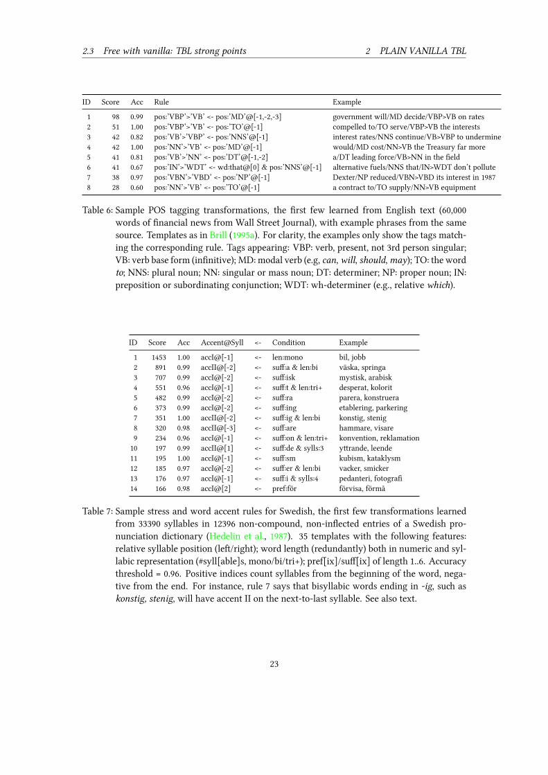
To illustrate, Table 6 gives the first few learned transformation rules from a widely used Englishcorpus and provides examples from the same text. All of the rules cited are general enough thatthey could be suggested as rules of thumb for human part-of-spee taggers (at least inexperiencedones, still trying to internalize and abstract the definitions). e accuracy figures simultaneouslyhints at the reliability of the rules thus learned (however, the actual scores of the rules are unim-portant, as they depend on the size of the training corpus and the specific tagset osen). Forinstance, rules 4-5 may in su a seing be paraphrased

“Uncertain if you look at a noun or a verb? Well, here is some help. If the previousword is a modal, su as can, should, may, then what you see is almost certainly averb. If one of the two previous words is a determiner (of whi the most commoncases are articles, su as a, an, the), then you probably look at a noun.”

e two things to note here is that these rules make perfect sense, and that they were extractedautomatically.For ease of exposition, we have used the same 26 templates as in Brill (1995a). Note, however,

that the alternative templates mentioned in Section 2.2.5 might permit even stronger generaliza-tions: rules 1 and 4 may possibly be merged, and the same goes for rules 2 and 8.Although of great practical value, the main point of POS tagging rules is seldom to provide

insights we did not have before. An example with different priorities is lexical stress and wordaccent prediction for Swedish. Somewhat simplified, ea Swedish non-compound, non-inflectedword has a particular syllable whi bears (main) stress. e stressed syllable is associated withone out of two possible word accents, corresponding to pit contours of the voice. Preciselyon what syllable stress is placed and whi of the two accents (Accent I or Accent II) thesyllable will have is mostly predictable from orthography, but not trivially so. ese are goodcircumstances for automatic detection of interesting rules. Due to reasons of space we cannotbe very detailed, but the main setup and results of a minimal su study are summarized inTable 7. Note the high value of the accuracy threshold, typical where the contents of rules aremore interesting than their scores.e words in the study were all non-compound and non-inflected, and several rules would

have looked different otherwise (for instance, rule 4 is not true for common inflected forms suas ’pulled’, talat ’spoken’, huset ’the house’). However, the results are already enough to rejectthe popular misunderstanding¹⁵ that Swedish basically has stress on the first syllable. As can beseen, almost all of the rules are conditioned on suffix, not on prefix, and stress placement is morereliably done from the end (this fact is reflected as negative indices in the accent/stressed syllablecolumn).

2.3.2 Compactness of learned representationA major aspect of interpretability, but also of great help in practical implementations (cf. Sec-tion 3.3.2), is the fact that the learned representation is very compact. As an extreme example, Brill(1994) presents a TBL system for unknown-word-guessing (i.e., assigning the most likely part-of-spee to words not in the system lexicon – for instance, reviving the examples from Section 1.2,

¹⁵Just to be clear: this is a popular misunderstanding, not a professional one.

22

2.3 Free with vanilla: TBL strong points 2 PLAIN VANILLA TBL

ID Score Acc Rule Example

1 98 0.99 pos:’VBP’>’VB’ <- pos:’MD’@[-1,-2,-3] government will/MD decide/VBP>VB on rates2 51 1.00 pos:’VBP’>’VB’ <- pos:’TO’@[-1] compelled to/TO serve/VBP>VB the interests3 42 0.82 pos:’VB’>’VBP’ <- pos:’NNS’@[-1] interest rates/NNS continue/VB>VBP to undermine4 42 1.00 pos:’NN’>’VB’ <- pos:’MD’@[-1] would/MD cost/NN>VB the Treasury far more5 41 0.81 pos:’VB’>’NN’ <- pos:’DT’@[-1,-2] a/DT leading force/VB>NN in the field6 41 0.67 pos:’IN’>’WDT’ <- wd:that@[0] & pos:’NNS’@[-1] alternative fuels/NNS that/IN>WDT don’t pollute7 38 0.97 pos:’VBN’>’VBD’ <- pos:’NP’@[-1] Dexter/NP reduced/VBN>VBD its interest in 19878 28 0.60 pos:’NN’>’VB’ <- pos:’TO’@[-1] a contract to/TO supply/NN>VB equipment

Table 6: Sample POS tagging transformations, the first few learned from English text (60,000words of financial news from Wall Street Journal), with example phrases from the samesource. Templates as in Brill (1995a). For clarity, the examples only show the tags mat-ing the corresponding rule. Tags appearing: VBP: verb, present, not 3rd person singular;VB: verb base form (infinitive); MD: modal verb (e.g, can,will, should,may); TO: the wordto; NNS: plural noun; NN: singular or mass noun; DT: determiner; NP: proper noun; IN:preposition or subordinating conjunction; WDT: wh-determiner (e.g., relative whi).

ID Score Acc Accent@Syll <- Condition Example

1 1453 1.00 accI@[-1] <- len:mono bil, jobb2 891 0.99 accII@[-2] <- suff:a & len:bi väska, springa3 707 0.99 accI@[-2] <- suff:isk mystisk, arabisk4 551 0.96 accI@[-1] <- suff:t & len:tri+ desperat, kolorit5 482 0.99 accI@[-2] <- suff:ra parera, konstruera6 373 0.99 accI@[-2] <- suff:ing etablering, parkering7 351 1.00 accII@[-2] <- suff:ig & len:bi konstig, stenig8 320 0.98 accII@[-3] <- suff:are hammare, visare9 234 0.96 accI@[-1] <- suff:on & len:tri+ konvention, reklamation10 197 0.99 accII@[1] <- suff:de & sylls:3 yrande, leende11 195 1.00 accI@[-1] <- suff:sm kubism, kataklysm12 185 0.97 accI@[-2] <- suff:er & len:bi vaer, smier13 176 0.97 accI@[-1] <- suff:i & sylls:4 pedanteri, fotografi14 166 0.98 accI@[2] <- pref:för förvisa, förmå

Table 7: Sample stress and word accent rules for Swedish, the first few transformations learnedfrom 33390 syllables in 12396 non-compound, non-inflected entries of a Swedish pro-nunciation dictionary (Hedelin et al., 1987). 35 templates with the following features:relative syllable position (le/right); word length (redundantly) both in numeric and syl-labic representation (#syll[able]s, mono/bi/tri+); pref[ix]/suff[ix] of length 1..6. Accuracythreshold = 0.96. Positive indices count syllables from the beginning of the word, nega-tive from the end. For instance, rule 7 says that bisyllabic words ending in -ig, su askonstig, stenig, will have accent II on the next-to-last syllable. See also text.

23

2.3 Free with vanilla: TBL strong points 2 PLAIN VANILLA TBL

guessing that staycation is a noun and defriend a verb). He quotes comparable performance forhis 148-rule system and an existing statistical unknown-word-guesser with 100, 000, 000 param-eters.

2.3.3 Competitive performancee rules induced by TBL may be interesting or at least interpretable reading to humans. Some-times, however, we don’t really care about su fringe benefits, but only about classification per-formance. As a stand-alone classifier, TBL generally reaes competitive results on a wide rangeof tasks, and state-of-the art for some. For other tasks, it lags somewhat behind the best statis-tical classifiers (at the time of writing oen Support Vector Maines). However, the trend inrecent years is that the best overall results are reaed not by single, stand-alone classifiers, butby combining several of these into ensemble learners. Su systems generally gain from diversityin their constituents, and indeed TBL oen contributes diversity. We return briefly to classifiercombination in Section 2.5.2.

2.3.4 Resistance to overtrainingFor most maine learning algorithms, a major problem is overtraining: the learned representa-tion describes random error or noise and thus fails to generalize outside the training data. Forinstance, it is very easy to detrimentally overfit decision trees, and careful measures must be takento avoid it (e.g., by growing the trees to completion and then ba-prune; or by performing somestatistical analysis before deciding that a node should be further split (Mitell, 1997)).TBL, by contrast, comes with an implicit ranking of the learned rules – they are automati-

cally ordered aer expected impact. is fact is the main reason for the method’s remarkableinsensitivity to overtraining.To be clear, TBL does overtrain – that is, if le to train until conclusion with a very low score

threshold, it will learn a large number of spurious, low-impact rules with no prospects of general-ization (most of whi will apply to a single site in the training corpus). But this trail of irrelevantrules does not significantly influence overall performance (in either direction). In case we pre-fer not seeing them anyway (perhaps because our main interest are the relevant rules only, andnot overall classifier performance), an efficient filter is just to raise the score threshold.¹⁶ Moresophisticated approaes are also conceivable, for instance by combining several TBL classifiers;we return to this topic in Section 2.5.2.Perhaps more disturbingly, irrelevant rules may conceivably emanate from unfortunate oices

of templates. Ramshaw and Marcus (1994) briefly investigate this issue. ey report on experi-ments with training in the presence of a template whi can safely be assumed to be irrelevant(su as “the POS of the word 37 positions to the le of the current”). When used in isolation, sua template naturally yields a large number of spurious rules; but when combined with relevanttemplates its influence is largely neutralized (Figure 3). eir conclusion is that the presence ofirrelevant templates will have lile impact, if only they are mixed with relevant ones. is is

¹⁶Exactly where to put it will depend on task, intention, corpus, tagset size etc. and may need some experimentation,but it need not be very high. As a comparison, Brill recommends a score threshold of 2 for his POS tagger designedfor English (typical tagset sizes 50− 150), on the corpus sizes of the mid-90’s (105 words).

24

2.3 Free with vanilla: TBL strong points 2 PLAIN VANILLA TBL

(a) 7 relevant templates

(b) 1 irrelevant template

(c) 7 relevant and 1 irrelevant templates

Figure 3: Learning curve in the presence of relevant and irrelevant templates. POS tagging ofGreek, 120kW. Solid line shows performance on training set, doed line performance ontest set, as a function of the number of learned rules. From Ramshaw and Marcus (1994).

useful knowledge in particular for cases where we are uncertain on what templates best catesthe dependencies of the problem – except training time, there is lile risk in specifying all possibletemplates we can think of (see also Section 3.1.2).We note that Ramshaw and Marcus (1994) are brief on their results, and in any case, more

investigation into TBL overtraining behaviour would be welcome, for differently sized data andtag sets and for other templates and tasks.¹⁷ In the words of Manning and Sütze (2001), itappears to be more of an empirical result than a theoretical one, and this judgment still seemsvalid in 2011.

¹⁷As stated in several places in this thesis, there is a preponderance for certain tasks and languages in the literature of

25

2.4 TBL vs. Decision Trees 2 PLAIN VANILLA TBL

2.3.5 Real-world objective functionTBL is an example of error-driven learning: the objective function¹⁸ that we wish to minimize isthe number of errors; and the evaluation function we use tooose between different solution can-didates is also typically (a monotonic function of) the current number of errors. us, our way ofevaluating competing rules or rule sets directly optimizes a measure in whi we have a practical,real-world interest, and differences in this measure correspond to differences in performance.By contrast, many classifiers use some less straightforward evaluation function (e.g., informa-

tion gain for decision trees) whi is only indirectly related to the classifier performance. Whilethe correlation of course is designed to be strong, it is not necessarily be perfect.e real-world relevance of the objective function also allows TBL training to be recast as an

optimization problem. is view allows the application of typical optimization teniques to thetask. For instance, Wilson and Heywood (2005) use genetic algorithms to minimize the errorfunction between reference and current corpus (see further Section 3.1.3).

2.4 TBL vs. Decision TreesAs several authors have noted (Ramshaw and Marcus, 1994; Brill, 1995a; Manning and Sütze,2001), TBL and decision trees (Breiman et al., 1984;inlan, 1993) have several commonalities. Aprototypical decision tree (DT) outputs a set of yes/no-questions whi can be asked about a sam-ple to get at its classification, very similar to the context part of a transformation rule (even moreso with templates of the form described in Section 2.2.5). e questions may refer to aributes ofthe sample being classified, but also to those of its neighbours. e TBL baseline simply corre-sponds to a default classification.e theoretical and practical differences between the two are important, however. For one

thing, DTs synthesize complex questions on any subset of the available aributes, whereas vanillaTBL requires the format of the rules to be specified by the templates.¹⁹ For another, arguablymore important, DTs have no (easy) way of saving away current hypotheses, and thus, the ques-tions cannot refer to intermediate predictions. us, in DTs (as in most other ML classificationsemes) classification is performed once and never anged. By contrast, TBL makes severalpasses through the data and later predictions may be improved based on earlier. As Ramshawand Marcus (1994) put it: “decision trees are applied to a population of non-interacting problemsthat are solved independently, while rule sequence learning is applied to a sequence of interre-lated problems that are solved in parallel, by applying rules to the entire corpus”. In fact, Brill(1995a) proves by induction that ordinary TBL rules are strictly more expressive than DTs: pre-cisely due to the possibility of leveraging intermediate results, there are classification tasks whican be solved by TBL but not by DTs. ese tasks may be of marginal importance, but it is notdifficult to find real-world cases where a solution with transformations is mumore concise andnatural than an equivalent DT. Brill exemplifies with tagging a word whose le neighbour is to,

Computational Linguistics, and sometimes “we have answered this question” is an inappropriate abbreviation for“we have answered this question for English”. See also Endnote v.

¹⁸Sometimes the terms “objective function” and “evaluation function” are used as synonyms. Here, we take the formerto describe the purpose to be fulfilled by any learner (generally minimizing or maximizing something), whereasthe laer refers to the quality of any particular solution, with respect to some representation.

¹⁹However, see also Section 3.1.3 and 3.1.2.

26

2.5 TBL in practice 2 PLAIN VANILLA TBL

whi may be an infinitival marker (to eat) and a preposition (to Scotland). In the first case, tois an excellent cue for verbs, in the second a good one for nouns. However, it may well be thatthe tagging of to itself into these two classes is unreliable. If so, TBL can automatically delay theexploitation of this cue until it has been more reliably established by other, intermediate rules,working on current predictions. By contrast, a DT whi exploits the same information is quitecomplicated and will likely contain duplicate nodes.e difference between DTs and TBL can also be viewed as one between stateless and stateful

classification. State is a mixed blessing, the discussions on whi fill up many a book in an averagecomputer science library.²⁰ Here, we will only note that a DT at work has no notion of order ortime, whereas TBL rule sets are strictly ordered,²¹ with current predictions representing state.Brill (1995a) mentions other practical advantages of TBL over DTs: beer resistance to problems

with sparse data and overtraining (a TBL rule has access to the entire training data when beingevaluated; by contrast, a DT recursively splits its training data in smaller subsets at ea node);the possibility to postprocess other output, and the transparency of the objective function. All ofthese have been treated in more detail in previous sections.As a final point, Hepple (2000) notes that for POS tagging, rule learning generally starts from a

very good baseline. is means that relatively few samples are retagged by rules, and fewer stillare retagged more than once. On these observations he bases two major simplifying assumptions:independence (rule interaction is ignored, so that early rules are not allowed to ange context forlater ones – in other words, all rules are learned in the context of the initial annotation); and com-mitment (any particular sample is anged by at most one rule). e rationale for the assumptionsis the massive gains in training time that they allow, and so we will revisit them in that context(Section 3.3.1). ey are mentioned here because with these assumptions, transformation rulesactually become a form of decision trees.

2.5 TBL in practice2.5.1 TBL as a standalone classifierTBL is a flexible and adaptable method, as witnessed by the large number of tasks it has beenapplied to. Table 8 lists a selection of tasks and associated central references. It is intended to besuggestive rather than exhaustive (see the bibliography mentioned on p. 10 for a somewhat moreserious aempt at completeness) but should cover the most diverse cases. e task names listed inthe table may not be very informative for readers who are not familiar with linguistic terminology.Indeed, some may be cryptic even to those who are: not all of the tasks listed are urgent oreven relevant for all languages, due to factors su as cross-linguistic variation, differences inwriting systems, and availability of appropriate data.v We refer to standard textbooks su asJurafsky and Martin (2008) for the interested;vi however, the details aren’t very important. emain point is that practically any level of language, spoken or wrien, is replete with symbolicclassification tasks based on sequential information in the local context; and with clever encoding,many problems can be made to fit this mould, some of them perhaps not obviously sequential.Indeed, in recent years the idea that all useful linguistic mappings can be cast as classification

²⁰e classic Abelson and Sussman (1996) is but one of them.²¹Brill (1995a) describes a transformation list as a processor, not a classifier.

27

2.5 TBL in practice 2 PLAIN VANILLA TBL

Task Ref

Part-of-spee (POS) tagging Brill (1993c, 1995a)Unknown word guessing Brill (1994); Mikheev (1997)Text unking Ramshaw and Marcus (1995)Prepositional phrase aament Brill and Resnik (1994)Parsing/grammar induction Brill (1996)Morphological disambiguation Oflazer and Tür (1996)Spelling correction Mangu and Brill (1997)Word segmentation Palmer (1997)Message understanding Day et al. (1997)Dialogue act tagging Samuel et al. (1998)Prosody prediction Fordyce (1998)Ellipsis resolution Hardt (1998)Word sense disambiguation Dini et al. (1998)Document format processing Curran and Wong (1999)Grapheme-phoneme conversion Bouma (2000)Grammar correction Hardt (2001)Handwrien aracter segmentation Kavallieratou et al. (2000)Regression Bringmann et al. (2002)Hyphenation Bouma (2003)Named entity recognition Florian et al. (2003)Compound segmentation Park et al. (2004)Disfluency detection Kim et al. (2004)Semantic role labeling Williams et al. (2004)Word alignment Ayan et al. (2005)Information extraction Nahm (2005)Biomedical term normalization Tsuruoka et al. (2008)Human activity recognition Landwehr et al. (2008)

Table 8: Sample TBL applications

28

2.5 TBL in practice 2 PLAIN VANILLA TBL

[light the candle] on [the table](a) light/I the/I candle/I on/O the/I table/I

light [the candle] on [the table](b) light/O the/I candle/I on/O the/I table/I

Figure 4: NP unks with encodings for light the candle on the table aer Ramshaw and Marcus(1995), before and aer applying the transformation I>O <- wd:the@[1]. I and Omarkinside and outside an NP, respectively. A third tag, B, is used for the first word in a newunk directly following another one, as in give/O the/I king/I his/B throne/I.

.

tasks, either as disambiguation or as segmentation, has gained support (Roth, 1998; Daelemans,1995). is assumption has opened several new fields to maine learning algorithms – TBL isjust one out of many.We will only give two examples here, osen to illustrate diversity in problem encodings. A

few more can be found elsewhere in this text (e.g., Section 3.5) and, of course, many others in thereferences of Table 8.In NP unking, a string of words is to be divided into non-overlapping, non-recursive subse-

quences corresponding to noun phrases (NPs).²² Figure 4 shows an example and a way (due toRamshaw and Marcus, 1995) of casting the task as a classification problem very mu like POStagging, with the same type of rules learned.emore intricate problem of parsing requires the encoding of recursive structures. e straight-

forward although somewhat un-linguistic solution proposed in Brill (1993b) is shown in Figure 5.

2.5.2 TBL in company: Ensemble learningLike any other classifier, in addition to its stand-alone use exemplified in the previous section,TBL may be used in combination with other classifiers. We have noted (Section 2.2.5) that aparticularly simple way of doing this is to use TBL as a post-processing, error-correcting step:since the algorithm assumes an initial-state annotation, but cares lile where it comes from, itcould just as well take the output of any other classifier as this initial baseline (e.g., Ruland, 2000;Wu et al., 2004). Besides (hopefully) boosting overall performance, TBL rules learned in this waymay provide some error analysis of the underlying classifier, summarizing the systematic errorsit makes.ere aremore sophisticated approaes than this to ensemble learning, i.e., combiningmultiple

classifiers into one in the hope of reaing beer predictive performance than could be obtainedfrom any of the constituent models alone. For instance, a typical commiee classifier mightcombine multiple ground-level classifiers (”commiee members”) with a higher-level classifier

²²ere is no single “correct” solution to this problem; practical needs will decide how to treat modifiers su aspossessives, prepositional phrases, or relative clauses. Of course, whatever the decision, it should be consistentlyheld to.

29

2.5 TBL in practice 2 PLAIN VANILLA TBL

lightthe

candleon the table

(a) ( light (the (candle (on (the table ) ) ) ) )

light

the candle on the table

(b) (light ( (the candle) (on (the table ) ) ) )

Figure 5: Parse trees with encodings for light the candle on the table aer Brill (1993b), beforeand aer applying the transformation delete a left paren to the right of a

determiner. Not shown are some behind-the-scene mainations to cater for paren-thesis balancing (see Brill (1993b) for details).

.

(”president”), with the idea that the different commiee members have complementary strengthsand weaknesses, and the job of the president is to learn when to trust whom. Ensemble learnersgenerally gain from being composed by classifiers with complementary strengths (Kuneva andWhitaker, 2003). To put it another way, ensemble learning is pointless if all component classifiersmake the same errors.Classifier combination largely falls outside the scope of this thesis; we will here only note that

TBL is different enough from most statistical sequential classifiers to make it a worthy memberof many commiees (e.g., Brill and Wu, 1998; Florian et al., 2003; Xin et al., 2006).

2.5.3 TBL in TBL companye aim of classifier combination of the type described in Section 2.5.2 is iefly to boost perfor-mance: combining the complementary strengths of several classifiers into a new and beer. iscan be done also with TBL as the single base learner. For instance, a number of slightly differentclassifiers can be induced from repeated resamplings of equally-sized subsets of the training data(bootstrap aggregating, or bagging (Breiman, 1996)). At classification time, ea TBL classifier isapplied independently, and its output taken as one vote for that class. Aer counting votes, themajority wins. Santos et al. (2010) claim to be the first to try this approa, for their ETL algorithm(Section 3.1.2). e resulting combined classifier is tried on text unking, named entity recogni-tion, and semantic role labeling. It shows substantial improvement on ETL alone, especially forthe semantic role labeling task, and aieves competitive or close to state-of-the-art results for allof them.

30

2.5 TBL in practice 2 PLAIN VANILLA TBL

Another idea for combining the knowledge of several TBL classifiers, apparently unexplored, isto merge the learned rule sequences, rather than weighing together the classifications they emit.Basically, rules whi are ranked high by all of the classifiers are highly likely to be relevant; butrules ranked low or (in particular) learned only by a few are likely not. e rule sequences mightbe combined by some rank combination measure and appropriate thresholds.²³As pointed out previously, TBLmay overtrain in the sense that many of its late learned rules are

spurious and irrelevant; its resistance to overtraining lies in the fact that su rules are automat-ically ranked as low-impact – they won’t influence performance mu in either direction. us,we might not expect a great performance boost from weeding out irrelevant rules. However, ifour main interest is the knowledge distilled, that is beside the point.

²³Finding combinations of ranked lists is a common problem in fields su as Information Retrieval and ComputationalBiology.

31

3 ADDING FLAVOUR

3 Adding flavour: TBL extensionsWe have showcased several desirable properties of the basic TBL method, but there is certainlyroom enough for development, improvement, and extension. In the following, we briefly surveythe most important new ideas for TBL: extending the domain of learned hypothesis (Section 3.1:to multidimensional learning, learning templates jointly and automatically, and learning withoutany templates at all); extending its range – its predictions – (Section 3.2: to probabilities, sets, andregressors); increasing efficiency (Section 3.3: in training and application); decreasing the needof supervision (Section 3.4); and facilitating declarative problem specification by domain-specificlanguages (Section 3.5).

3.1 Extending the hypothesis domain3.1.1 Multidimensional learningMany real-world applications involve more than one subtask – perhaps one classifier to assignparts-of-spee to ea word and another for finding binary braning trees. A simple way ofdoing su combined tasks is to put the appropriate classifiers in a pipeline, resulting in a strictlyfeed-forward system, where the outcome of task k cannot influence the outcome of task k − 1.For very different and/or truly independent tasks, this may be the best way. A variation is beamsear, where we keep n > 1 hypotheses from early steps and defer complete disambiguationuntil later.However, when two tasks A and B are somewhat dependent we may benefit more from mul-

titask learning (Caruana, 1997). Intuitively, if we can expect that solutions to A may provideuseful information for solving B and vice versa, then it would be beer not having to imposean ordering of these tasks on the system, but rather solve them in parallel. In that way, the easycases (of both A and B) may provide information for the more difficult ones (of both A and B).Two su interrelated tasks are POS tagging andunking – dividing sentences into larger, non-overlapping units (somewhat like parsing without tree structures; we saw a simpler special caseof unking in Figure 4). Here, easy cases are for instance POS and unks whi can be reliablypredicted directly from word forms.Indeed, multitask learning on well-osen representations may be worthwhile even when we

are not really interested in solving all of the tasks – learning POS by jointly learning unks isconceivably easier than learning POS alone.One way to set up su a joint classifier is to simply create a new derived feature as the concate-

nation of the features we wish to combine. However (in analogy with computing joint probabilitydistributions) this may cause problems of data sparseness with many types of data. Unusual jointvalues will have unreliable estimates, and joint values whi do not occur in the training datawill never be predicted.A beer way for many purposes is to let the tasks share a common representation and let ea

classifier work on it simultaneously. TBL is well suited for joint learning in this way. Florian andNgai (2001) point out the fewanges needed to themain algorithm, mainly small modifications tothe scoring function f . As stated before (Section 2.2.5), to guarantee termination, f needs to assignpositive values only to rules whi actually decrease the current error count. is requirement

32

3.1 Extending the hypothesis domain 3 ADDING FLAVOUR

is easily met also in a multidimensional seing, by just leing f taking more than one field intoaccount:

f(r) =∑s∈C

n∑i=1

wi · (Si(r(s))− Si(s))

Here,

• C is the set of training samples (the training corpus);

• r is a candidate transformation rule to be scored;

• r(s) is the sample whi is the result of applying r to sample s;

• n is the number of fields (tasks);

• wi is an optional weight or priority (see below) for task i;

• Si(s) is an indicator of the current classification of sample s for task i: 1 if correct, 0 if not.

e weights wi could be used to manually assign priorities to ea subtask. ey might also beinitialized from training data based on the counts of correct and incorrect sample classificationsfigures for ea field – say, as constants for the entire training session, or as per-iteration valuesto be recalculated and reassigned aer ea rule application. Differently weighted aributes areapparently an unexplored option.To conclude, in the TBL case, multidimensional learning can be seen as a generalization of one

of the previous key arguments for the method: we can use intermediate results to guide laterpredictions. e multidimensional addition is that su intermediate results may refer to morethan one feature.

3.1.2 Automatic template learningTemplates are the main tool for embedding and encoding domain knowledge in TBL. On the otherhand, they can be tedious or difficult to produce. e tediummay to a large extent be alleviated byautomation (e.g., the template compiler described in Lager (1999b)). As we have seen, overtrainingis seldom a problem in TBL, so unnecessary templates will mostly only affect training time. Agreater concern is insufficient domain knowledge: for less well-understood problems, it may bedifficult to know where to start. Learning templates automatically then becomes an aractiveoption.Curran and Wong (2000) envision “evolving templates that ange in size, shape and number

as the learning algorithm continues”, starting from few and simple templates whi are gradu-ally refined into (or replaced by) more complex ones in a data-driven fashion. ey present noimplementation, but they show empirically that the number of conditions in the templates andtheir specificity (e.g., words rather than tags) increase during learning – simple templates withfew conditions are most efficient early on, but later more complex templates tend to pay off beer.However, the task providing their data is again POS tagging for English; it would be desirable tosee their claims corroborated for other tasks and data sets.

33

3.1 Extending the hypothesis domain 3 ADDING FLAVOUR

Figure 6: Template extraction from decision tree. First, the leaves and the labels of the learnedtree are discarded. In the resulting subtree, ea path from the root to an internal nodecorresponds to a template (right). Redrawn from Santos (2009).

Less abstractly, Milidiú et al. (2007) implement a genetic algorithm (Mitell, 1997) for automatictemplate learning. eir system shows impressive performance but their reported setup suffersfrom slow training; with the TBL algorithm as the fitness function, training must happen for eaindividual of the population, for ea generation. For anything but the smallest feature sets, thisrapidly becomes intractable.A recent approa (Santos and Milidiú, 2009; Santos, 2009), dubbed “Entropy-based Transfor-

mation Learning” (ETL), instead constructs templates from a decision tree (DT) trained on thetask at hand. A DT can be thought of as a series of yes-no questions asked about an object to beclassified, with the questions ordered in terms of descending Information Gain (IG) (see Mitell(1997); inlan (1993), cf. also Section 2.4). e main idea behind ETL is that the features whiare addressed by the DT-induced questions on task X are likely to make up a good set of TBLtemplates for X . Ea path from the root to any internal node of the learned DT corresponds toa specific series of questions and thus a specific set of features (Figure 6) – i.e., a template.Some care needs to be taken to avoid typical DT training problems. e standard algorithms

will strongly favour high-dimensional features – for instance, word identity, rather than part-of-spee. e version of ETL described in Santos (2009) tries to control this by sorting the values ofa high-dimensional feature in decreasing IG order and replace all except the z top-scoring oneswith a dummy value, where z is a parameter of the algorithm. Furthermore, as discussed inSection 2.4, decision trees are inherently stateless and has no notion of a “current” classification.For the purposes of template generation, ETL solves this by introducing the true value of theclassifications in the context (but not for the current object).Santos andMilidiú (2009) report excellent results for ETL on a number of tasks (Fernandes et al.,

34

3.1 Extending the hypothesis domain 3 ADDING FLAVOUR

Figure 7: Bit string encoding of one particular rule in TBL by genetic algorithm. Any subset of tagswithin a window of current position±3 can be encoded, replacing a manually specifiedtemplate set. From Wilson and Heywood (2005).

2010; Milidiú et al., 2008, 2010; Santos et al., 2008, 2010). e approa has apparently so far onlybeen used by this single group of researers; a more thorough evaluation will have to wait.

3.1.3 Template-free TBLAn even more radical approa than automatic template learning is TBL without any templates atall. Wilson and Heywood (2005) suggest a genetic algorithm (Mitell, 1997), whi (in contrast tothe previous genetic approa byMilidiú et al. (2007)) does away with templates entirely. Instead,an entire sequence of rules corresponds to one individual in the population; and one individual isa collection (384, in the experiment) of rules represented as a fixed-length bit strings (Figure 7).Although an undeniably novel approa, several critical oices are tuned to the specifics of

POS tagging (in particular, for English). us, the rather small tagset size is part of the encodingassumptions: it is not clear how the method would handle a larger target set or many-valuedfeatures (as well may be crucial in other tasks). It is also unclear how it would respond to alower-scoring baseline. e paper does not exemplify any rules learned; that would otherwisehave made interesting comparisons with standard TBL.TBL without manually specified templates seems in particular well-motivated when the oice

of templates is problematic, perhaps due to poor understanding of the domain. is is hardly thecase for POS tagging in English, so template-less genetic algorithms may have more potential forother tasks. Performance is also quite a bit lower (the authors report 89.8% from a baseline of80.3%; Brill’s original algorithm scores 97.0% on the same corpus).Ba et al. (2008) suggest template-free learning by an exhaustive sear through the power set

of a user-defined feature space, where ea subset of features is allowed to generate one rule forea error. e paper leaves quite a few questions unanswered and we won’t discuss it further.²⁴

²⁴For one thing, it seems contradictory on how output rule lists are actually compiled. ere is also no information

35

3.2 Extending the hypothesis range 3 ADDING FLAVOUR

3.2 Extending the hypothesis range3.2.1 Predicting probabilities: Soft classificatione vanilla output of a TBL classifier is one class per sample, with no information as to the uncer-tainty of the class osen. ese are hard decisions, commiing the system to a single possibilitywith no information as to the certainty of the oice.Probabilistic systems, by contrast, make so decisions, providing confidence measures for ea

classification. Confidence measures are useful for many purposes, and indispensable for some.For instance, in ensemble systems (Section 2.5.2), the member classifiers may disagree; it is thenvery useful to know howmu they are willing to insist. In active learning, the idea is to minimizemanual effort; su systems use confidence measures to identify the most uncertain (and thus, tothe system, most informative) samples and ask the annotator for their classification. For some ap-plications hard decisions are simply inappropriate. Larger, multi-component systems (e.g., speerecognizers) are generally built frommany smaller modules whi all deal with probabilistic inputand output (say, as probability distributions, or as ranked candidate lists).Two notable aempts have been made to add enhance TBL with probabilistic classification.

ey share the basic idea of spliing the training data into equivalence classes: all the sampleswhi have been tagged X for reasons Y are considered together. en probabilities can beestimated for ea equivalence class by standard means (e.g., maximum likelihood estimation,probably with some smoothing).vii

Florian et al. (2000) gives an algorithm for transforming a learned rule list into an equivalentdecision tree, and then taking the leaves of that tree as equivalence classes. ey note that theequivalence classes thus constructed will tend to vary a lot in size. In particular, with a goodbaseline, the equivalence class of samples to whi no rules apply at all can easily make up mostof the corpus, and the probability estimates of that class will be close to those arrived at withoutany learning at all. To remedy that, the learned tree is treated as a (highly accurate) prefix, whosepaths are grown further with standard decision tree learning methods (inlan, 1993).Santos and Milidiú (2007) instead construct equivalence classes from the baseline classification

and rule traces – for instance, all samples that had initial classification and were later touedby rules 11, 57 and 88 form an equivalence class of their own. e problem of unevenly sizedclasses is solved by subdividing on manually specified auxiliary features. e authors claim asignificant improvement over Florian et al. (2000) on comparable tasks. eir method arguablyadheres beer to the inherently stateful TBL paradigm (cf. Section 2.4), but seems to involve moretask-specific hand-coding (the auxiliary features to specify) as well as more assumptions on thedata (the relevance of the initial classification).In any case, probabilistic TBL is an interesting subject, with several unexplored paths. For

instance, it is not clear what influence a dumber initial classification (forcing more samples to betoued by some rule) or a higher accuracy threshold (inducing a bias for more accurate rules)would have on the quality of the estimates learned with one method or the other.

on running time, nor any performance comparisons with ordinary-templated TBL – only modest error correctingscores on good or excellent baseline systems are listed.

36

3.2 Extending the hypothesis range 3 ADDING FLAVOUR

3.2.2 Predicting sets: Constraint grammarWe have already mentioned (Section 1.3) that one of the most successful POS taggers for Englishis the originally hand-wrien rule system EngCG (Karlsson et al., 1995). CG stands for ConstraintGrammar. Very briefly (and somewhat simplified), su a system starts with initializing a can-didate set of tags for ea word to the set of all possible tags for that word (as found in a lexicallookup, or in a reference corpus). en it traverses a list of rules, ea formalizing some require-ment, or constraint, on the solution.²⁵ Tags not fulfilling a certain constraint can be removed fromthe candidate set (the last tag should not be removed, however).Ideally, only one correct tag will remain when all rules have been applied. In reality, of course,

some samples will have had the correct tag removed in the process and others will still havemore than one possibility le. us, the evaluation measure of a CG-like system needs to beadapted accordingly. It is usually calculated on precision and recall instead of percentage correct– typically as the F1 score borrowed from Information Retrieval.²⁶A great advantage of CG-like systems is that they can exploit negative information, say “amodal

verb is never followed by an adjective” as easily as positive. On the other hand, a major drawbais the reliance on every single rule being correct: in contrast to other variations of TBL, it is notpossible to let later rules correct the mistakes of earlier ones. If the correct tag is erroneouslyremoved from a sample, there is no magic bla hat from whi it could be reproduced. us, thisstyle of learning will strongly emphasize rules with perfect or almost perfect accuracy.CG rules were originally specified by hand, but naturally, several aempts have been made

to extract them automatically from a corpus (e.g., Samuelsson et al., 1996). e question ofinterest here is how to do so by TBL. Lager (1999b) shows that this can be aieved by con-ceiving of transformations not as replacement rules but rather as set operations. He incorpo-rates this style of learning in his µ-TBL system. Especially important are reduction rules, whiremove an element from a set if it is not the last (otherwise, they do nothing). An exampleof su a reduction rule is “reduce the current tag set of a word with tag if the word im-mediately to the le is uniquely tagged as ”. In the µ-TBL formalism this rule would readpos:red vb <- unique pos:dt@[-1] and it would probably be derived from the templatepos:red A <- unique pos:B@[-1]. Lager (2001) explores this learning style for the case ofPOS tagging. e results are promising, but prohibitively slow for scaling up: from amodest-sized240kW corpus with 15 templates, the TBL Constraint Grammar learner described in Lager (2001)learns 4866 rules in three weeks (!). A more efficient algorithm for CG-style TBL is clearly crucialif the method is to gain wider usage.A final disadvantage of CG-style systems is that their output is made up of sets, and using it

as part of a larger system thus presupposes that interfaces of later links are prepared to handleunranked sets as input. In an increasingly probabilistic view on knowledge induction and transfer,this assumption may be problematic.

²⁵e “Grammar” part of the term is less informative and reflects the early uses of the approa – it is certainlyconceivable to use it on problems outside grammar or POS tagging.

²⁶http://en.wikipedia.org/wiki/F1_score

37

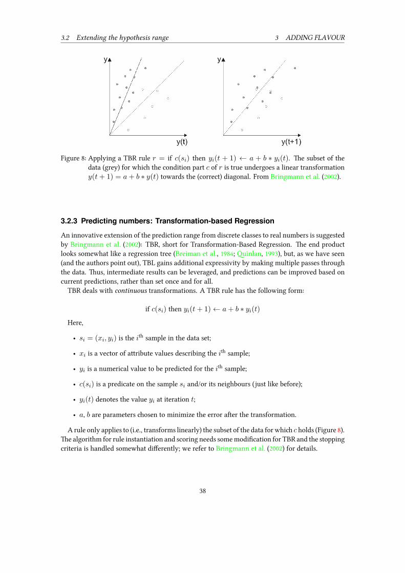
3.2 Extending the hypothesis range 3 ADDING FLAVOUR

Figure 8: Applying a TBR rule r = if c(si) then yi(t + 1) ← a + b ∗ yi(t). e subset of thedata (grey) for whi the condition part c of r is true undergoes a linear transformationy(t+ 1) = a+ b ∗ y(t) towards the (correct) diagonal. From Bringmann et al. (2002).

3.2.3 Predicting numbers: Transformation-based RegressionAn innovative extension of the prediction range from discrete classes to real numbers is suggestedby Bringmann et al. (2002): TBR, short for Transformation-Based Regression. e end productlooks somewhat like a regression tree (Breiman et al., 1984; inlan, 1993), but, as we have seen(and the authors point out), TBL gains additional expressivity by making multiple passes throughthe data. us, intermediate results can be leveraged, and predictions can be improved based oncurrent predictions, rather than set once and for all.TBR deals with continuous transformations. A TBR rule has the following form:

if c(si) then yi(t+ 1)← a+ b ∗ yi(t)

Here,

• si = (xi, yi) is the ith sample in the data set;

• xi is a vector of aribute values describing the ith sample;

• yi is a numerical value to be predicted for the ith sample;

• c(si) is a predicate on the sample si and/or its neighbours (just like before);

• yi(t) denotes the value yi at iteration t;

• a, b are parameters osen to minimize the error aer the transformation.

A rule only applies to (i.e., transforms linearly) the subset of the data for whi c holds (Figure 8).e algorithm for rule instantiation and scoring needs somemodification for TBR and the stoppingcriteria is handled somewhat differently; we refer to Bringmann et al. (2002) for details.

38

3.3 Improving efficiency 3 ADDING FLAVOUR

Two drawbas are difficult to avoid when leaving the world of discrete classifiers and enteringthe continuous regression domain. First, overtraining becomes a mu more pressing issue. isis a standard problem, with several common solutions. e one proposed by Bringmann et al.(2002) is similar to that oen used in pruning decision trees: partition the available training datainto a development and a validation set, and then prune the tree/truncate the list to the smallestone within a certain error (e.g, one standard error) from the best one on the validation set. Second,arguably a greater loss, TBR sacrifices a large part of rule interpretability (cf. Section 2.3.1): themeaning of rules in the form above is difficult to grasp. Although the top scoring rules may makesome intuitive sense, rule effect is generally cumulative, and later rules whi linearly transformthe output of earlier ones make no more sense to humans than does any other bla-box method.It should be noted, however, that these downsides are no worse for TBR than for other regres-

sors. Performance-wise, the authors report TBR to be competitive with state-of-the-art regres-sion learning algorithms on difficult sequential regression tasks (predicting segment durationsfrom phonological features, and predicting three main musical parameters of expression in pianoplaying).

3.3 Improving efficiency3.3.1 Efficiency in trainingOne major disadvantage of the TBL algorithm of Section 2.2 is the very slow training. Brill’soriginal implementation (in C) was generously made available on the web early on and was oenused for POS tagging as a preprocessing step in other applications. However, although it containedclever optimizations, it commonly needed days of training time. For instance, Ngai and Florian(2001b) report 38 hours training for the simple task of POS tagging on a 1 million word corpus,whi still is small by the standards of 2011.²⁷e time complexity of the TBL training phase is difficult to specify. e worst-case analysis

is clear, but rather absurd: a corpus of size N where all initial tags are incorrect and the correcttags are all unique. us, no possible rule will ever correct more than a single error. Given Ttemplates, we get O(NT ) rules to oose from in ea iteration,²⁸ and since there are N errorsto correct and no rule corrects more than one of them, we will have to learn O(N) rules. us,training takes O(N2T ) time, and no indexing semes will improve the situation. Of coursenobody would want to try maine learning on su a data set, but it at least establishes an upperbound. We could also consider O(N) a lower bound – we won’t need the templates to find outthat there are no errors to correct, but we clearly need to look at the entire corpus.e average case (whi is of course what we are really interested in: a corpus with some

but not complete regularity and a meaningful baseline whi does not get everything wrong) ismore difficult to pinpoint. e most informative statistic is the number of learned rulesR, whi,however, will vary a lot with the task at hand: it will grow with the size of the corpus N , with

²⁷More complex tasks are rather worse; and the situation is further exacerbated when a TBL system is used as one ofseveral base learners in iterating ensemble learners.

²⁸Templates may contain alternative positions, su as pos:A@[1,2] meaning some pos tag A at position 1 or 2.Given a specific sample with erroneous classification, su a template will usually generate more than one rulethat corrects it. We will disregard that in the discussion here. At any rate, considering the maximum contextwidth a constant, O(T ) templates will still generate O(T ) rules per application site.

39

3.3 Improving efficiency 3 ADDING FLAVOUR

the initial number of errors E, and with the number of templates T , but not independently andnot very predictably with either.Roughly, with O(E) errors in the current corpus, learning a single rule with the greedy but

otherwise naive algorithm of Section 2.2 will involve identifying O(ET ) candidates in timeO(N + ET ), scoring them in O(ENT ), piing the best in O(ET ), and applying it in O(N).e expensive scoring step can be optimized by sorting the candidates according to their descend-ing good application counts gi, keeping a best score sb, and interrupting the scoring as soon asthe gi falls below sb. is optimization, present in most implementations, is very efficient forthe first few rules, when scoring can be interrupted early, but grows increasingly inefficient asrule scores drop, when a large fraction of the rules will have to be investigated. As a result, thismethod typically finds the initial rules inO(E0T ) but then slows down toO(ERNT ) as trainingprogresses (where R is the number of rules learned and Ei is error count aer applying i rules).An early aempt to speed up training is represented by Ramshaw and Marcus (1994). ey

proposed an elaborate indexing seme and minimal state updates between iterations. In aninitial phase, the corpus is traversed linearly twice, once to identify O(ET ) positive rules forea error and ea template; once to identify the negative application sites of those rules. Asa result, ea rule in effect has a list of (pointers to) the samples it may be applied to, and easample a list of (pointers to) the rules that can be applied to it. e list of rules is scored and sortedand the top scoring rule is selected. When applied, ea of its sites of application can be accessedin constant time, and all the rules affected by the ange of corpus state can in turn be efficientlyupdated. e initial phase takes O(ENT ), then the application of ea of the R rules starts atO(ET ) for the first one and approaes O(T ) as the number of samples anged Cr (at most2gr) approaes the constant score threshold. us, once the index is built, no linear searesneed to be performed in the corpus.²⁹ Unfortunately, this method consumesO(NT ) memory (orpossiblyO(ET ), with judicious filtering of rules whi have higher negative than positive score).is makes it infeasible for most real-world tasks with more than a handful of templates.Ngai and Florian (2001b) propose what is essentially a mu more memory-friendly simplifi-

cation of the algorithm of Ramshaw and Marcus (1994). Instead of storing O(E) pointers forea rule in O(ET ) space, they only store the good/bad count (gr, br). At the cost of a linearsear per iteration, the rule-to-score list then becomes mu smaller and the sample-to-rule listsuperfluous. We defer the details of this algorithm to the next section, where we rephrase it fora declarative paradigm; here, we only note that aer building and indexing the initial rule listthe top scoring rule can be found in constant time, applied in O(N), and the state updated inO(N + CTw), where w is the width of the widest template context and C is the number ofapplication sites. Towards end of training, this approaes O(N + STw), where S is the scorethreshold.An entirely different approa to improving training efficiency is Monte Carlo (MC) sampling

of the rule space (Samuel, 1998a; Carberry et al., 2001). In ea iteration, for ea error discoveredin the current corpus, a fixed number of templatesK are osen randomly and used to generatecorrecting rules. In effect, we get an unbiased sample of (the currently interesting part of) the rule

²⁹Previously unseen rules may occasionally be created in the neighbourhood of application sites, to correct errorsintroduced by the application. Scoring su rules will need linear corpus scans. In our experience, creation of newrules can usually be disabled without performance loss.

40

3.3 Improving efficiency 3 ADDING FLAVOUR

space. Usually the highest-scoring rule will be the best one, and almost always one of the best. Aswe have mentioned (p. 20), small reorderings of good rules are usually not crucial: when severalrules have about the same efficiency, either they correct the same error, in whi case we couldpi any of them; or they correct different errors, in whi case they are usually independent andtheir local ordering relative to ea other is of lile consequence. Running time does not dependon the number of templates, and thus MC sampling is particularly useful where the number oftemplates is high – for instance, when the feature-space is inherently high-dimensional and/orthe domain is not (yet) completely understood.For POS tagging, Carberry et al. (2001) show impressive speedups (two orders of magnitude)

with no concomitant drop in performance. ere might be tasks where performance is moreimpacted. For instance, low-scoring rules yield smaller samples and thus are scored with lesscertainty than high-scoring, for well-known statistical reasons; also, if there are very many ruleswith approximately the same score, true ordering requirements among them are more likely tobe violated. us, the approa may be more problematic when the bulk of the error correctionis catered for by a large number of low-scoring rules. At any rate, MC sampling oen deservesconsideration when non-determinism is acceptable.Yet another approa are the explicitly stated independence assumptions proposed by Hepple

(2000), that we met in Section 2.4: independence (no rule interaction with respect to the conditionpart of a rule – all rules are learned in the context of the initial annotation); and commitment(at most one ange per sample). Hepple describes two algorithms based on them (ICA and ICP:Independence, Commitment, and either Append or Prepend, depending on whether the rules areapplied in the learned order or in reverse). e simplified learning shows very impressive speedups(several orders of magnitude).Clearly, the validity of the IC assumptions depend very mu on the problem. Some problems

are not sequential; some are sequential, but can reasonably be treated as if they weren’t; somecannot be handled as sequential without major information loss. Furthermore, the error rate ofthe baseline is crucial. Fewer errors of course mean fewer and lower-scoring rules to learn; thus, itis generally far between rule application sites and rules will not interfere. Poorer baselines meanmore rule interaction. For POS tagging, the performance loss is slight (and probably outweighedby the possibility of training on mu larger data sets). For several other tasks, IC is significantlyworse (Ngai and Florian, 2001b).

3.3.2 Efficiency in applicatione naive application of a set of learned rules to new data is by sequential substitution, one ruleat a time. us, it takes O(RKn) time to apply R rules requiring context of sizeK to a input ofsize n. is may be good enough for some purposes, but when the rules for instance describe apreprocessing step for data-intensive applications (say, information extraction), it is too slow.Roe and Sabes (1995) apply finite-state algebra to the rule sequences. ey show that a

single learned TBL rule ri may be regarded as a non-deterministic transducer ti. It follows thatthe entire set of rules corresponds to the composition of su transducers, whi in itself is a non-deterministic transducer T . Not all non-deterministic transducers can be determinized. However,the authors show that T , resulting from composing fixed-width context TBL rule sequences, ac-tually can (except perhaps for practical limitations). is yields a transducer with O(n) perfor-

41

3.4 Widening the bolene: Unsupervised learning 3 ADDING FLAVOUR

mance in the size of the input, with very low constants – in fact, the run time of their POS taggeris dominated by the data transfer time from disk.

3.4 Widening the bottleneck: Unsupervised learningClassification tasks are by definition supervised – they depend on annotations provided by hu-mans beforehand. For instance, the original TBL algorithm presupposes for the learning step areference corpus where ea element in ea of the sequences, whatever they might represent, hasbeen tagged with its true class. Su data sets are costly to construct. If one can get away withless expensive resources, it is of course useful. Brill (1995a) proposes an extension to TBL POS-tagging, where the baseline annotation of a word is created by simply listing all of its possible tagsin some fixed but arbitrary order, disregarding context. For instance, the baseline annotation ofthe will likely be the singleton DT; but export will perhaps list VP|VBP|NN (present-tense, non-3rdperson singular verb, as in Cubans export sugar; infinitive verb, as in Cubans want to export moresugar ; or noun, as in Cuban export of sugar will increase). e system treats this three-item set asa single tag like any other except that it can be decomposed for scoring (see below). e templateslook just like before, for instance A > B <- tag:@[-1].Rule scoring has to be adapted: since we do not have access to truth, we cannot simply count

errors corrected. We can, however, score rules according to how efficiently we expect them toreduce uncertainty. is can be done in many ways. Brill (1995a) uses the following formula³⁰ toscore rules derived from the template A > a <- C (ange A to a in context C , where A is anambiguous tag and a is one of its possibilities):

score(A, a,C) = U(a)

[UC(a)

U(a)−max

UC(Y )

U(Y )

]Here, U(X) is the total number of words in the corpus uniquely tagged X , UC(X) is the

number of words uniquely tagged X in the context C , and Y is a variable ranging over theambiguous tags of A except a.In the example above, with the specific context c = dt@[-1] (determiner one step to the le),

this amounts to

score(||, , c) = U()

[Uc()

U()−max

(Uc()

U(),Uc()

U()

)]score(||, , c) = U()

[Uc()

U()−max

(Uc()

U(),Uc()

U()

)]score(||, , c) = U()

[Uc()

U()−max

(Uc()

U(),Uc()

U()

)]

Terms of the form UC(X)U(X) range from 0 to 1, and thus the second factor ranges from −1 to 1.

Given the context of the example, any real-world corpus will find it close to −1 for the first twocases and close to 1 for the third.

³⁰although differently presented, in our opinion less clearly

42

3.5 Abstracting the problem: Template compositionality and DSLs 3 ADDING FLAVOUR

Word POS True unk Initial unk

O art i ialuno noun i iesqueceu verb o oo art i icaderno noun i ide prep i icaligrafia noun i iamarelo adj i oem prep o icasa noun i i

Figure 9: Chunking the Portuguese sentenceO aluno esqueceu o caderno de caligrafia amarelo emcasa ’e student le the yellow calligraphy notebook at home’. Example from Santosand Oliveira (2005).

With only four templates, Brill (1995a) reports rather impressive 96% (from a baseline of 90%).However, he simplistically assumes a complete lexicon. Aone and Hausman (1996) extend themethod for Spanish to cope with unseen words, and Beer (1998) generalizes and parameterizesthe approa, allowing compositional templates and different scoring semes. For instance, thescoring seme above disregards all ambiguous contexts, whi presupposes that there are enoughof the non-ambiguous ones; but one might also want to include ambiguous tagging in the scoring(and then probably weighted according to degree of uncertainty).We may extrapolate this idea to Constraint Grammar-style rules (Section 3.2.2) by considering

all tags as sets, possibly singletons, and have the transformations implement set operations ratherthan replacements (e.g., reduction: remove a tag from the possibilities). is allows mu easierexploitation of negative information and might be a way to explore unsupervised transformation-based learning also for the Constraint Grammar paradigm. e sear space is very large, though,and the problematic training time of TBL-CG needs to addressed first.

3.5 Abstracting the problem: Template compositionality and DSLsSantos and Oliveira (2005) apply TBL to unking (p. 29) in Portuguese, but find that traditionaltemplates are too inflexible to cat important lexical relations. As example, they give the relationbetween preposition em ’on’ and the verb esqueceu ’le’ (Figure 9). With the verb esquecer ’leave’,a prepositional phrase headed by em is generally an adverb, does not belong to the object nounphrase, and should be tagged o. As a remedy, they propose a widened “constraint atomic term”,where templates can express things like “condition on value x of feature X of the current word’sclosest neighbour whi has value y for feature Y”. By way of example, they give a template ofthe form (where [x;y] indicates a closed interval from x to y, inclusive):

43

3.5 Abstracting the problem: Template compositionality and DSLs 3 ADDING FLAVOUR

word[0;0](pos=prep) word[−2;−10]³¹ (pos=verb)

From the data in Figure 9, su a template would allow the system to induce the rule

word[0;0](pos=prep)=em word[−2;−10](pos=verb)=esqueceu –> chunk=O.

is rule should be read “if pos[0]=prep and word[0]=em, and, for the first item in the closedinterval [-2;-10] where pos=verb, word=esqueceu; then ange the value of feature chunk to O

for the target item”. e authors then suggest algorithms to implement their new extension.We mention this idea not because we find it a good one, but to illustrate a point. In our view,

the suggested extension is at best an acceptable solution to the wrong problem, a problem whiwas phrased too specifically to begin with.³² Mu beer than adding one ad-hoc feature or an-other to the syntax of TBL templates is to make the templates themselves form a lile language,with values, abstractions, and combinators as befit the domain. Su a language is known as adomain-specific language (DSL); in the words of van Deursen et al. (2000), a DSL is a “small, usu-ally declarative, language that offers expressive power focused on a particular problem domain.”An appetizing alternative to implementing a DSL from scrat is to extend some suitable baselanguage with domain-specific constructs. In this way, all features of the base language can bereused. More importantly, so can the users’ knowledge of it. Su an extension can range in com-plexity from some preprocessing step up to a complete embedding (an embedded DSL (Hudak,1996, 1998)).To our knowledge, there is only one aempt at a DSL for TBL: the template language of the

μ-TBL system (Lager, 1999b). A moderately complex template description for a particular task(dialogue act tagging) in this system is given in Figure 10.μ-TBL is implemented in the logic programming language Prolog, and its template language

is just a Prolog extension (by preprocessing). Figure 10 (as well as the examples below) maynot be very informative for readers unfamiliar with that language,³³ and we must anyway omitsome details on data format, argument passing to the auxiliary predicates, etc.³⁴ e point shouldbe clear, however: some features are given directly in the data representation, while others arecomputed dynamically by auxiliary predicates of arbitrary complexity, but the templates use bothkinds and can’t tell the difference between them. If we were to trade space for time by includingsome of the computed features in the data representation instead, the templates wouldn’t notice.Furthermore, just as important, the templates themselves are compositional; they are ordinaryProlog terms and can be assembled and disassembled by the standardmeanisms of the language.We will return to μ-TBL in Section 5. Here, we will only take the Portuguese example as a

minimal coding exercise in a DSL (fictive, but perfectly conceivable and not mu beyond that ofFigure 10).

³¹Starting two to the le (-2) rather than with the le neighbour (-1) leaves a spot for the direct object, as in don’tleave keys on the table.

³²We unfortunately find this a common paern. Non-compositional problem encodings (oen with too mu focuson performance) tend to create monolithic systems with hard-coded oices: hard to extend, hard to experimentwith, hard to understand.

³³Good books on Prolog, in suggested reading order, are Closin and Mellish (1994); Covington et al. (1997); Bratko(2001); Sterling and Shapiro (1994); O’Keefe (1990)

³⁴see http://www.ling.gu.se/~lager/Mutbl/mutbl_system.html

44

3.5 Abstracting the problem: Template compositionality and DSLs 3 ADDING FLAVOUR

%%% DATA REPRESENTATION %%% AUXILIARY PREDICATES

s(1,speakerA). u_mem(Position, Word) :-

da(1,acknowledge). u(Position, Words),

da(acknowledge,ready,1). member(Word, Words).

u(1,[ehm, right]).

u_first(Position, Word) :-

s(2,speakerA). u(Position, [Word|_]).

da(2,acknowledge).

da(acknowledge,instruct,2). u_bigram(Position,(Word_i, Word_j)) :-

u(2,[you,start,at,the,caravan,park]). u(Position, Words),

nextto(Word_i, Word_j, Words).

s(3,speakerB).

da(3,acknowledge). s_change(Position, Change) :-

da(acknowledge,acknowledge,3). ( s(Position, Speaker),

u(3,[ok]). Position1 is Position-1,

%... s(Position1, Speaker)

-> Change = false

; Change = true

).

%%% TEMPLATES %Condition the transformation rule on...

da:A>B <- da:C@[-1]. % the previous dialogue act

da:A>B <- da:C@[-1,-2]. % any of the two previous dialogue acts

da:A>B <- da:C@[-1] & da:D@[-2]. % both of the two previous dialogue acts

da:A>B <- u_first:W@[0]. % the first word in current utterance

da:A>B <- u_mem:W@[0]. % any word in current utterance

da:A>B <- u_bigram:W@[0]. % any two adjacent words in current utt.

da:A>B <- s:C@[0]. % the current speaker

da:A>B <- s:C@[0] & u_mem:W@[0]. % any combination of word and speaker

da:A>B <- s_change:C@[0] & u_mem:W@[0]. % any word in current utterance, if a

% speaker change has just occurred

Figure 10: Dialogue act tagging in μ-TBL: data representation, auxiliary predicates, annotatedtemplates. Adapted excerpt from Lager and Zinovjeva (1999). Abbreviations: s:speaker,u:uerance, da:dialogue act, mem:member.

First, assuming a data representation similar to what we have seen (Figure 11, top), we findthat the example template can be expressed with our existing toolkit (Template 1a in Figure 11,middle).Of course, if our DSL allows partial application, there is no reason to hardcode the direction,

the bounds, or the POS we look for. Instead, we could parameterize them in the generally usefulpredicate closest/6 (Figure 11, boom). is allows Template 1a to be rephrased as Template 1b.More interesting, with closest/6 in place, our DSLmay now let us replace the direction to searin (left) and the POS tags to sear for (verb and prep) with variables, as usual to be filled inwith the values whi make the strongest predictions. For instance, Template 2 in Figure 11expresses something like “condition the unk tag ange on the current word, its part-of-spee

45

3.5 Abstracting the problem: Template compositionality and DSLs 3 ADDING FLAVOUR

%%% DATA REPRESENTATION

wd(1, o ). pos(1, art). chunk(1, i). chunk(i, i, 1).

wd(2, aluno ). pos(2, n ). chunk(2, i). chunk(i, i, 2).

wd(3, esqueceu). pos(3, v ). chunk(3, o). chunk(o, o, 3).

%...

%%% TEMPLATE 1a

chunk:A>B <-word:W@[0] & pos:prep@[0] & closest_left_verb_2_10:VerbWord@[0].

%%% AUXILIARY PREDICATE

closest_left_verb_2_10(Position, Word) :-

between(2, 10, I),

Position1 is Position - I,

pos(Position1, verb),

!,

word(Position1, Word).

%%% TEMPLATE 1b

chunk:A>B <-word:W[0] & pos:prep@[0] & closest(left, verb, 2, 10):VerbWord@[0].

%%% TEMPLATE 2

chunk:A>B <-word:W[0] & pos:POS1@[0] & closest(Dir, POS2, 2, 10):POS2Word@[0].

%%% AUXILIARY PREDICATE

closest(left, POS, ClosestBound, FarthestBound, Position,Word) :-

between(ClosestBound, FarthestBound, I),

Position1 is Position - I,

pos(Position1,POS),

!,

word(Position1, Word).

closest(right, ...) %identical, except Position1 is Position + I

Figure 11: DSL templates for Portuguese unking. Data representation (top) and auxiliary pred-icates in different degree of abstraction (see text).

P1, and the word (within a window to either le or right) whi belongs to a part-of-spee thatP1 usually has informative associations with.”To be sure, Template 2 in Figure 11 is not necessarily a good one. If nothing else, it is almost

certainly inefficient: depending on the size of the corpus and the tagsets, the combinatorial ex-plosion may render it unusable in practice. However, decisions on whi seares to perform andwhi to prune are beer le to the user than to the designers of the template language.We could go on and parameterize thewindow edges, or, even beer, replace thewindow entirely

with some predicate “earlier in the sentence”. Wewill stop here, however, in the belief that we havedemonstrated the expressivity and conciseness a DSL can gain by reusing well-known conceptsand constructs of the base language.

46

4 FAST, DECLARATIVE TBL

Figure 12: Data flow of TBL training, extended with state (dashed boxes) ruleScores

4 Fast, declarative TBLAs pointed out, one of the major problems of the standard TBL training algorithm is the very slowlearning phase. Section 3.3.1 discussed some proposed improvements. Here, we look closer at oneof those, due to Ngai and Florian (2001b). Like many other aempts at improving efficiencywe have seen in TBL (and, to be sure, in Computer Science in general), it is based on the ideaof using state to avoid recalculation. In the TBL case, this involves generating all potentiallyhelpful rules once, computing some amount of information for ea, and saving that informationas part of global state. en, aer ea rule application, it is enough to update state minimally,instead of regenerating new rule candidates from scrat. Figure 12 shows the system aritectureaugmented with state (cf. Figure 2).e algorithm byNgai and Florian (2001b) resembles the one described by Ramshaw andMarcus

(1994). In that case, however, we saw (Section 3.3.1) that the amount of information kept traof for ea rule turned out to be prohibitively memory-expensive for most practical uses. Bycontrast, in the algorithm described here, ea rule r is associated only with two integers: thecounts for good and bad applications.In the following, we give an algorithmic overview, and we present a novel, more declarative

rephrasing of the originally strongly imperative algorithm. Our version is slightly slower than the

47

4.1 Notation 4 FAST, DECLARATIVE TBL

original³⁵ (replacing hash-based maps with functional, tree-based counterparts will oen comewith a O(log(N)) cost, although there might be alternatives in specific cases), but it is beeradapted for declarative languages and (in our opinion, anyway) easier to understand. In addition,in contrast to the imperative variation, ours is parallelizable (although, admiedly, the speedupsmeasured so far fall quite a bit below their theoretical ceiling, see Section 4.6).

4.1 Notatione following notation and definitions are used throughout this section (from Ngai and Florian(2001b), slightly adapted):

• S is the sample space – a set of mutually independent sequences of positive length;

• C is the set of possible classifications of a sample;

• C[s] is the current classification of sample s;

• T [s] is the true classification of sample s;

• p is a predicate on S;

• r is a rule: a pair (p, t) of a predicate p and a target t (a class label);³⁶ given a rule r, wewrite pr and tr for its predicate and target, respectively;

• good(r) is the count of good applications (successful error corrections) of rule r;

• bad(r) is the count of bad applications (newly introduced errors) of rule r;

• R is the set of all rules that we keep tra of (a subset of the total rule space);

• GBi[r] denotes the current counts (good(r), bad(r)) of rule r in iteration i;

• GBi is used for the current good/bad counts for all rules in iteration i;

• A rule r applies to a sample s if pr(s) and tr 6= C[s].

Any other notation will be introduced as needed.

4.2 Algorithmic overviewClearly, if we have GBi in some appropriate data structure, it is easy to efficiently find the best-scoring rule bi in ea iteration i. e question then reduces to two subtasks (dashed boxes inFigure 12): how do we initialize the state and how do we update it; or, more declaratively spoken,how do we get GB0; and how do we get to GBi+1 from GBi, given bi.e first subtask is very similar to what we have seen many times before.

³⁵For time complexity estimations, we refer to Section 3.3.1.³⁶Note that rules in this formalism correspond to the templates of Table 4, not to those of Table 1.

48

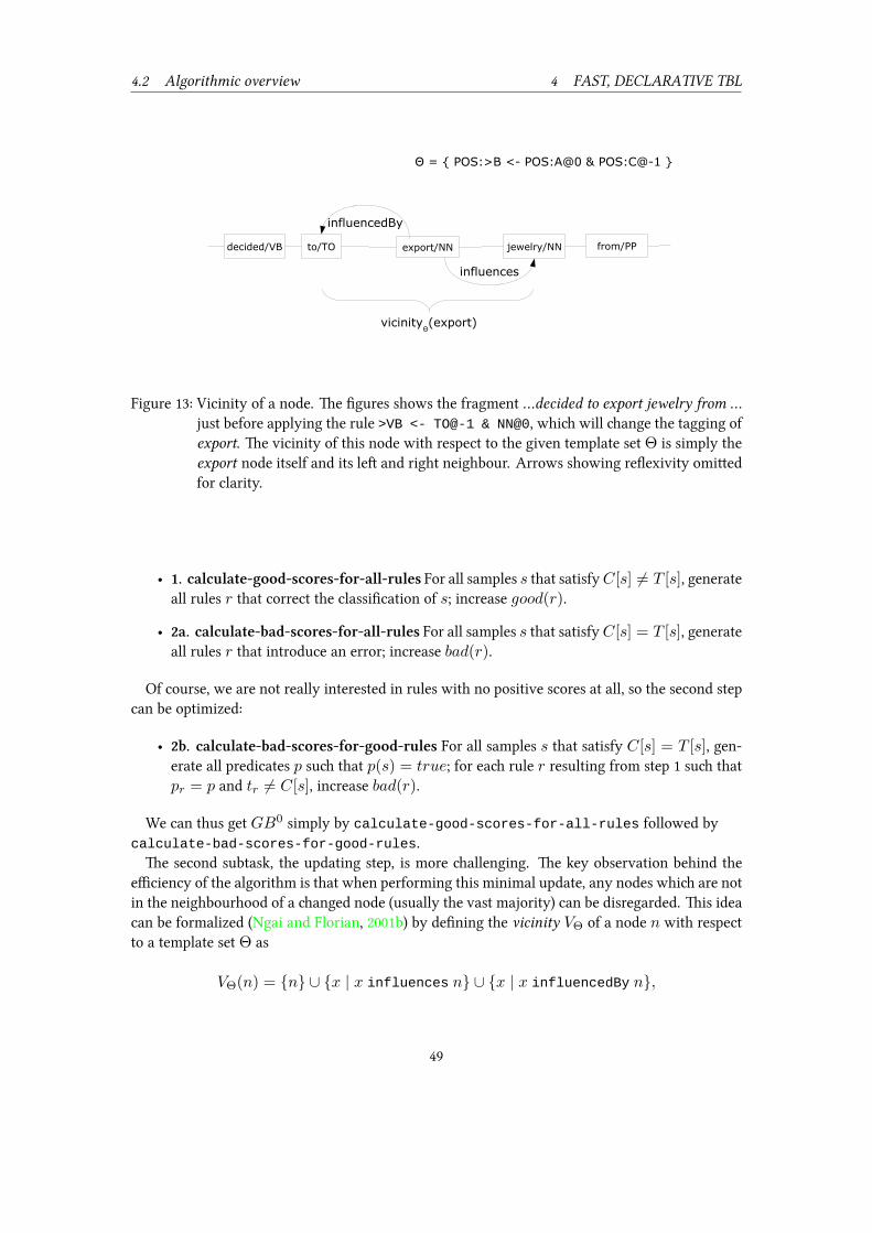
4.2 Algorithmic overview 4 FAST, DECLARATIVE TBL

Figure 13: Vicinity of a node. e figures shows the fragment …decided to export jewelry from …just before applying the rule >VB <- TO@-1 & NN@0, whi will ange the tagging ofexport. e vicinity of this node with respect to the given template setΘ is simply theexport node itself and its le and right neighbour. Arrows showing reflexivity omiedfor clarity.

• 1. calculate-good-scores-for-all-rules For all samples s that satisfyC[s] 6= T [s], generateall rules r that correct the classification of s; increase good(r).

• 2a. calculate-bad-scores-for-all-rules For all samples s that satisfyC[s] = T [s], generateall rules r that introduce an error; increase bad(r).

Of course, we are not really interested in rules with no positive scores at all, so the second stepcan be optimized:

• 2b. calculate-bad-scores-for-good-rules For all samples s that satisfy C[s] = T [s], gen-erate all predicates p su that p(s) = true; for ea rule r resulting from step 1 su thatpr = p and tr 6= C[s], increase bad(r).

We can thus get GB0 simply by calculate-good-scores-for-all-rules followed bycalculate-bad-scores-for-good-rules.e second subtask, the updating step, is more allenging. e key observation behind the

efficiency of the algorithm is that when performing this minimal update, any nodes whi are notin the neighbourhood of a anged node (usually the vast majority) can be disregarded. is ideacan be formalized (Ngai and Florian, 2001b) by defining the vicinity VΘ of a node n with respectto a template set Θ as

VΘ(n) = {n} ∪ {x | x influences n} ∪ {x | x influencedBy n},

49

4.3 A low-level view: Updating GB 4 FAST, DECLARATIVE TBL

where x influences y if there is any template θ ∈ Θ su that x occurs in the CONDITION of θand y in the ACTION. e converse relation, of course, is influencedBy. Vicinity is illustrated inFigure 13.

4.3 A low-level view: Updating GB

e update step for iteration i as proposed by Ngai and Florian (2001b), given a rule br to apply,involves identifying all samples whi are in the vicinity of any node anged by br , and todistinguish all the different ways these anges influence the to-be-finished rule counts GBi.is operation is complicated and we will not delve into the details here. Imperative pseudocodefor their entire algorithm is given in Figure 14 (lines 1-5 correspond to the initialization of GB0;lines 9 and below perform updating of GBi).

4.4 A high-level view: Computing GB∆

Although very useful, in our experience the amount of book-keeping detail makes the implemen-tation of the algorithm of Figure 14 difficult to get right. Furthermore, it is geared towards datastructures whi use memory destructively;³⁷ thus, it is difficult or impossible to parallelize.It turns out that the algorithm can be made quite a bit easier to understand when viewed at a

higher level of abstraction. In addition, if we sti to purely functional data structures, we canmake it parallelizable³⁸ Even in an imperative paradigm, with destructive memory access and thuslesser prospects on parallelism, the gained clarity might be reason enough to prefer the alternativeview.Crucially, we prefer to think of the updating step as performing exactly the same operation as

the initial rule scoring, except on a set of independent (hence the potential for parallelization)subcorpora – namely, the union of all vicinities of all application sites of the best-scoring rule b.To see how this view is useful, we first define an addition operation for rule counts. Given two

rule counts GBa and GBb we define their sum to be the multiset sum GBa+b = GBa ] GBb.at is, GBa+b is the mapping su that

GBa+b[r] = GBa[r] +GBb[r]

where r ranges over the rules in either GBa or GBb; and GB[x] is taken to be 0 whenever xis not in the map. Rule count subtraction is defined analogously.Second, we define the partitioning and the filtering of a data set D (a set of independent se-

quences of positive length) with respect to a rule r and a template set Θ:

partitionr,Θ(D) = (DVΘ(r), D¬VΘ(r))

filterr,Θ(D) = DVΘ(r)

³⁷e authors suggest a two-level hash, keyed on pr and tr as the main data structure for GB.³⁸Hopefully it will also be easier to integrate into a declarative DSL, although we will not pursue that path further

here.

50

4.4 A high-level view: Computing GB∆ 4 FAST, DECLARATIVE TBL

For ea sample s that satisfies C [s] 6= T [s],generate all rules r that correct the classification of s; increase pos (r).

For ea sample s that satisfies C [s] = T [s]generate all predicates p s.t. p (s) = 1; for ea rule r s.t. pr = p and tr 6= C [s] increase neg (r).

1: Find the rule b = argmaxr∈R f (r).

If (f (b) < reshold or corpus learned to completion) then quit.

For ea predicate p,let R (p) be the set of rules whose predicate is p (i.e. R (p) = {r|pr = r}).

For ea samples s, s′ s.t. C [s] 6= C [b (s)] and s′ ∈ V (s):

• If C [s′] = C [b (s′)] then

– For ea predicate p s.t. p (s′) = 1

* If C [s′] 6= T [s′] then· If p (b (s′)) = 0 then { decrease pos (r), where r = [p, T [s′]], the rule created withpredicate p and target T [s′]; }

* Else· If p (b (s′)) = 0 then for all the rules r ∈ R (p) s.t. tr 6= C [s′] decrease neg (r);

– For ea predicate p s.t. p (b (s′)) = 1

* If C [b (s′)] 6= T [s′] then· If p (s′) = 0 then { increase pos (r), where r = [p, T [s′]]; }

* Else· If p (s′) = 0 then { For ea rule r ∈ R (p) s.t. tr 6= C [b (s′)] increase neg (r);

Else

– For ea predicate p s.t. p (s′) = 1

* If C [s′] 6= T [s′] then· If p (b (s′)) = 0 ∨ C [b (s′)] = tr then decrease pos (r), where r = [p, T [s′]];

* Else· For ea rule r ∈ R(p) s.t. tr 6= C [s′] decrease neg (r);

– For ea predicate p s.t. p (b (s′)) = 1

* If C [b (s′)] 6= T [s′] then· If p (s′) = 0 ∨ C [s′] = tr then increase pos (r), where r = [p, T [s′]];

* Else· For ea rule r ∈ R (p) s.t. tr 6= C [b (s′)] increase neg (r);

Repeat from step 1:

Figure 14: e FnTBL algorithm (Ngai and Florian, 2001b).

51

4.4 A high-level view: Computing GB∆ 4 FAST, DECLARATIVE TBL

Figure 15: Partitioning a corpus (the Penn treebank) with respect to a rule b and a template setΘ.Bla for DVΘ(b), grey for D¬VΘ(b) (see text).

Here, we abuse the V (· ) notation somewhat by expanding it from samples to rules: DVΘ(r)

consists of all vicinities of all application sites of r, taken to be elements of a sequence if theyare so inD (with any overlapping sequences merged – no samples are duplicated). Analogously,D¬VΘ(r) is everything that did not fit – either subsequences whi were le over when vicinitiesof longer ones were removed, or other unanged sequences whi didn’t contain any applicationsites to boot. Normally, |DVΘ(r)| � |D¬VΘ(r)|. See Figure 15.We now assume that we have a template setΘ, a data setD, a rule countGBi

D for the currentiteration i, and a best-scoring rule b whi partitions D into DVΘ(b) and D¬VΘ(b). e goal is tocalculate the net effect of applying b,GBi

∆ = GBi+1−GBi, in terms of this partition. First, wenote that in any iteration i, the good and bad counts contained in GBi

D can be wrien (leavingthe dependence on Θ implicit, to reduce cluer)

GBiD = GBi

D¬V (r)+GBi

Π(r) +GBiDV (r)

(7)

where GBiΠ(r) is a residual term needed to account for sequence boundaries (it depends on

templates whi applied before the split but not aer or vice versa). us,

GBi+1D = GBi+1

D¬V (r)+GBi+1

Π(r) +GBi+1DV (r)

(8)

e key insight here is that application of b has no influence on either GBΠ(r) or GBiD¬V (r)

;

thus GBi+1Π(r) = GBi

Π(r) and GBi+1D¬V (r)

= GBiD¬V (r)

. Subtracting (7) from (8) yields

GBi∆ = GBi+1

D −GBiD = GBi+1

DV (r)−GBi

DV (r)(9)

52

4.5 Implementation notes 4 FAST, DECLARATIVE TBL

In summary, we can calculate the update GBi∆, needed as a consequence of applying the rule

b, by:

1. extracting the subcorpusDV (b) of vicinities of all applications sites of b;

2. score all relevant rules forDV (b);

3. apply b to (a copy of)DV (b) and score the result;

4. subtract the result of (2) from the result of (3).

An outline of the algorithm in functional-style pseudocode³⁹ is given in Figure 16. Several de-tails are omied; thus, we assume the procedures given in Section 4.2 (with the obviousanges forthe functional paradigm to accept necessary parameters and to return values); furthermore, corpusfiltering, rule count addition, and rule count subtraction as described above; and finally some sen-sible definitions of findBestRule (cf. page 18), applyRule (cf. page 20), and terminationReached(cf. page 21).

4.5 Implementation notesWe implemented the algorithm just described in the functional language Haskell (Peyton Joneset al., 2003).⁴⁰ Here, we collect a few random observations from the process.

• e algorithm requires efficient access to the best-scoring rule and to the scores of ea rulegiven (pr, tr). In a declarative seing, this can be acquired by pairing a functional heap(Okasaki, 1998) and a tree-based map.

• e idea behind the optimization we applied in the initialization step (2b in Section 4.2,calculate-bad-scores-for-good-rules) is useful also when scoring subcorpora, butthe -good-rules part then need to refer to the good rules for the entire corpus. (epseudocode of Figure 16 ignores this optimization, to reduce cluer).

• Occasionally, application of a rule will create the opportunity for an entirely new rule r′,previously unseen. Even if good(r′) falls below the scoring threshold s in the current itera-tion (and r′ thus is not likely to be used, as far as we presently can tell), more opportunitiesmay turn up in later iterations.

However, introducing new rules can be very expensive, as there are no minimal updatesto apply: to score any rule created aer the initialization stage we will need to sear theentire corpus linearly (see next section for some practical measurements). In our experience,disallowing the introduction of new rules does not affect performance noticeably. It wouldbe unwise, however, to make statements of all possible scenarios, so a more flexible solutionis to parameterize rule creation by a threshold. New rules not reaing this threshold willbe ignored. A reasonable value is s or a bit above it. Ngai and Florian (2001b) are not clearon how they handle this point.

³⁹Essentially Haskell with over-explicit function names, java-style signatures in function definitions, and no worriesabout IO.

⁴⁰Haskell tutorials in suggested reading order are Hudak et al. (2000); ompson (1999); Hudak (2000); O’Sullivan et al.(2008).

53

4.5 Implementation notes 4 FAST, DECLARATIVE TBL

scoreInitialCorpus(Corpus cps, Templates tpls) = goodBadScores

where

goodScores = calculateGoodScoresForAllRules(cps, tpls)

goodBadScores = calculateBadScoresForGoodRules(cps, tpls, goodScores)

scoreSubcorpus(Corpus subCps, Templates tpls) = goodBadScores

where

goodScores = calculateGoodScoresForAllRules(subCps, tpls)

goodBadScores = calculateBadScoresForAllRules(subCps, tpls)

nextGoodBadCount(Rule bestRule, RuleCount goodBad, Corpus cps) = goodBad’

where

subCps = filter(bestRule, cps)

subCps’ = applyRule(bestRule, subCps)

deltaScores = scoreSubcorpus(subCps’) - scoreSubcorpus(subCps)

goodBad’ = goodBad + deltaScores

tbl(Corpus cps_0, Templates tpls) = until(terminationReached, iter, initialState)

where

terminationReached(Corpus cps, RuleCount goodBad, Rules rls) = ...

iter(Corpus cps, RuleCount goodBad, Rules rls) = (cps’, goodBad’, rls’)

where

bestRule = findBestRule(goodBad)

rls’ = append(rls, bestRule)

cps’ = applyRule(bestRule, cps)

goodBad’ = nextGoodBadCount(bestRule, goodBad, cps)

initialState = (cps_0, goodBad_0, rules_0)

where

goodBad_0 = scoreInitialCorpus(cps_0, tpls)

rules_0 = []

-- until(pred, iter, a)

-- yields the result of repeatedly applying function iter until pred holds,

-- with a as the initial value

Figure 16: Fast, declarative TBL in functional-style pseudocode. Names beginning with upper-case leers informally denote types; with lower-case they denote values. x and x’

have the same type, usually understood as x’ being a modified version of x

54

4.6 Algorithm time and memory consumption 4 FAST, DECLARATIVE TBL

In addition, any aempt to parallelize code inevitably will bring up design oices. Haskell is apurely functional language with referential transparency, whi puts it in a beer position thanmost to explore the increasing number of cores on modern hardware. Nevertheless, compilers forparallel programming is work in progress in any language. If there are any silver bullets, theyhaven’t been found yet, mu less fired. e main problem is to find, ahead of time, the right sizeof the work unks: if too small, the bookkeeping cost will dwarf any parallelization gain; if toobig, some of the cores may idle their time away while their colleagues are sweating over the task.Haskell offers three mainmeanisms for programmer-controlled parallelism. One uses explicit

control with transactional memory (similar to other languages). Another, Data Parallel Haskell(Chakravarty et al., 2007), is more original. It offers nested data structures whi are specially builtto be traversed in parallel, with ea core executing exactly the same instruction (a single programcounter). e third (Trinder et al., 1998) is mu more lightweight; it amounts to speculativelyannotating data structures where the compiler should sear for parallel opportunities.With the data description introduced in the previous section, we know that ea updating step

involves a large number of independent and not entirely trivial tasks. is knowledge is a goodbase for aspiring to parallelism gains (today, but hopefully even more so with the even smartercompilers of tomorrow). For the purposes here, we will not be very ambitious: we will be satisfiedwith a demonstration that su gains actually are possible, rather than trying to maximize them.us, we restrict ourselves to the simple annotation seme of Trinder et al. (1998). For a moreserious implementation (e.g., aiming at the same performance ballpark as the existing FnTBLimplementation) we would have considered Data Parallel Haskell, whi can be expected to scaleto a mu larger number of cores.

4.6 Algorithm time and memory consumptionTo measure running times, we used the original setup of Brill (1995a): 26 templates, score thresh-old 2, accuracy threshold 0.5, the Wall Street Journal corpus. e aieved tagging accuracy wasnot of interest (and the same in all cases, for a given corpus size). e experiments were run on adual-core computer.⁴¹ For ea corpus size, we recorded the time needed to produce the first rule(Time0, see Figure 17), the time to finish training where new rules were allowed to be created inea iteration (TimeN-create) and where new rules were disallowed (TimeN-nocreate). For com-parison, we implemented the basic TBL algorithm (including the common optimization describedon p. 40) and ran it on the corpus sizes it could reasonably handle (TimeN-Brill).As can be seen, for this setup, allowing new rules almost doubled the running time, with no

gain. Brill’s original algorithm is asymptotically slower, as expected.Our aempt at parallelization (Figure 17, right) resulted in a speedup on the order of 30%. is

is quite a bit from the theoretic maximum, but given the effort (about 20 lines of code), we at leastfind it interesting.⁴²Figure 18 (le) gives an idea of the state size. e thing to note is that state grows sublinearly

in the size of the corpusN . is means that the size of the corpus dominates that of the state and

⁴¹ghc 6.8 and 6.10, Ubuntu 8.10 on a Lenovo T400, Intel Core Duo, 2.26 GHz, 4GB RAM)⁴²Note that the more recent Haskell compiler actually performed worse. We have not looked further into this maer,

but it does strengthen the impression that parallelization is a triy business.

55

4.6 Algorithm time and memory consumption 4 FAST, DECLARATIVE TBL

that total memory usage thus is linear in N (Figure 18, right), whi is the best one could hopefor.

Figure 17: Algorithm performance: Running time (seconds) as a function of corpus size. Le:comparison with Brill’s original algorithm. See text for details. Right: parallel perfor-mance, one and two cores used on two different Haskell compilers.

Figure 18: Memory usage as a function of corpus size. Le: state size (nodes in tree). Right:maximum memory residency (MB).

56

5 CONCLUSION AND FUTURE DIRECTIONS

5 Conclusion and future directionsIn this thesis, we have provided a survey of Transformation-Based Learning. We have done sowithout aiming at full formal detail, but hopefully we have been explicit enough to provide a self-contained introduction to the basic method, and to the most important of its later developments.Where the full story is needed, we believe that the pointers provided will be helpful, as well asthe comprehensive bibliography.⁴³ Furthermore, we have tried to fill a small gap by rephrasing astate-of-the-art training algorithm for declarative languages.In the introduction, in addition to these two concrete aims, we also expressed a rather vague

hope of promoting the general interest in TBL. As we have mentioned, TBL is almost unheardof outside the linguistic world. Indeed, the absence of non-linguistic applications in Table 8 isstriking, the only exceptions being Bringmann et al. (2002) and Landwehr et al. (2008). We don’tsee any particular reasons why this should be so. It is true that the kind of local dependenciesTBL is especially suited for exploiting are particularly common in language, but they certainlyoccur elsewhere.Although rarely sufficient by themselves, good introductions and good toolkits are helpful when

propagating ideas. While any of several sources (including, perhaps, this thesis) may serve thefirst role, the casting of the second is less clear. What qualifications should we look for in thecandidate? A prerequisite for making it in the non-linguistic world is clearly that there are nolimiting, specifically linguistic assumptions on data or tagsets. Actually, removing suhardcodedassumptions is likely to benefit linguists, too, who are looking for new application domains for awell-tested tenique.For a second requirement, we have made no secret of our view that one of the most flexi-

ble ways to interact with a toolkit is via a DSL (Section 3.5), whi can hide any amount ofimperative mainations behind the appropriate, high-level abstractions of the domain. A well-designed, syntax-light DSL whi covers the relevant concepts of the domain should generally beunderstandable and usable by a domain expert who is not a programmer (especially if it is of thedeclarative kind). Yet, it exposes all the power of the system (and its underlying base language,when built as an extension of an existing one) to the experienced user.On the wish list we may also find features su as unicode compliance, open source, prospects

of parallelization, performance, and many other things. Different projects will weigh these factorsdifferently and we will not dwell on them here.With su a list of desiderata, what candidates will we currently find on the world wide web

marketplace? As it turns out, “currently” is not very different from ten years ago. To our knowl-edge, there are currently four TBL implementations publicly available on the web: Brill (C),⁴⁴FnTBL (C++),⁴⁵ NLTK (Python),⁴⁶ and μ-TBL (Prolog).⁴⁷Brill was the first implementation, but it is hard-coded for POS tagging and now mostly of

⁴³See footnote on p. 10.⁴⁴e original page has disappeared, but a mirror of the Brill tagger at its latest version is at

http://www.tech.plym.ac.uk/soc/staff/guidbugm/software/RULE_BASED_TAGGER_V.1.14.tar.Z

⁴⁵http://www.cs.jhu.edu/~rflorian/fntbl/, latest update 2001⁴⁶http://www.nltk.org/, Natural Language Toolkit, general tools for language processing; the toolkit is continu-

ously updated, but there has been no non-trivial anges to the TBL module at least since version handling startedin 2005

⁴⁷http://www.ling.gu.se/~lager/mutbl.html, latest update 2000

57

5 CONCLUSION AND FUTURE DIRECTIONS

historical interest. e others all have different strengths and weaknesses. FnTBL is the fastestand widely used. It implements several of the extensions of Section 3, but it is not so easy toextend or experiment with for non-C++ programmers. e TBL implementation present in NLTKis part of a larger toolkit for natural language processing, actively developed. It thus offers APIsto all kinds of language-processing modules and utilities. However, its TBL part is very basic andclearly geared towards the specific task of part-of-spee tagging. With proper generalization andextension, its impressive infrastructure would make it an interesting tool for TBL applications, butcurrently it seems less useful than it could be.In our view, μ-TBL is the most interesting, and we will describe its pros and cons in somewhat

more detail. It is well-documented and has been used in several real-world projects. It offersan interactive interface and a scripting language for automation. Code for compiling learnedrules into blazingly fast FSTs (Section 3.3.2) can be generated automatically. It contains, to ourknowledge, the only aempt to learn Constraint Grammar rules by TBL.Most importantly, as we have already seen exemplified (Figure 10), its template specifications

form a declarative DSL, expressive but concise. It should be reasonably understandable to domainexperts without insights into Prolog or even programming. Still, templates may use arbitraryProlog code for complex tasks.⁴⁸To be sure, the toolkit has a lot of improvement potential, too. It was developed under Sicstus, a

commercial and relatively expensive implementation of Prolog for whose availability no guaran-tees can be made; ports between Prolog systems are usually possible, but tiresome. Besides Brill’soriginal, it includes the fast randomized training algorithm due to Samuel (1998b) mentioned inSection 3.3.1, but none of the sometimes preferable alternatives (e.g. Ramshaw and Marcus, 1994;Ngai and Florian, 2001b; Hepple, 2000; Santos andMilidiú, 2007). Data is input as Prolog databases,rather than in more widely used formats su as csv or XML. All data partitioning into train andtest set must be done by preprocessing. e latest code ange is from 2000: thus, the systemsuffers slightly from general bit rot (no unicode; poor use of later hardware, especially memory).It should be commended for its design around exangeable training algorithms, but this API stillmakes unfortunate assumptions on the template format (cf. Table 1 vs. Table 4).Furthermore, μ-TBL does of course not contain any of the post-2000 developments (and only

a few of the earlier ones) described in Section 3. A list of useful extensions includes probabilis-tic TBL (Section 3.2.1), multidimensional TBL (Section 3.1.1), template-free TBL (Section 3.1.3),TBL with automatically learned templates (Section 3.1.2), TBR (Section 3.2.3), unsupervised TBL(Section 3.4), and means of automatically building ensembles (Section 2.5.3).⁴⁹Leaving current and planned toolkits aside, we may briefly speculate on future general de-

velopments of the TBL method itself. We have mentioned several areas whi seem to deserve

⁴⁸As a remark, Prolog may seem like an odd oice of implementation language: generally speaking, Prolog tends tofit very well to some problems and very poorly to others, with the traditional, strongly imperative phrasing of TBLrather belonging to the second group. However, Prolog is an excellent base language for a declarative DSL behindwhi any amount of imperative detail can be hidden. e details of the hiding is the problem of the implementer,not the user of the DSL.In addition, it might well be worthwhile to look for other phrasings than the imperative ones. Lager (1999b)

presents an implementation whi is derived from a logical interpretation of TBL rules; and, by way of a practicalargument, Lager (1999a) describes an implementation of a system based on this idea whi is an order of magnitudefaster than Brill’s original, with the Prolog source code fiing on a single page.

⁴⁹We are aware that writing su lists is quier than implementing them.

58

5 CONCLUSION AND FUTURE DIRECTIONS

wider use (e.g., ETL, Section 3.1.2; TBR, Section 3.2.3; probabilistic TBL, Section 3.2.1; ConstraintGrammar-TBL, Section 3.2.2) and others whi apparently have been explored lile or not at all(weights in multidimensional learning, Section 3.1.1; unsupervised Constrained Grammar-TBL,Section 3.4; alternative scoring semes, Section 2.2.5; TBL rule purification in ensembles, Sec-tion 2.5.3). Time will tell whi ones of these are worth their salt.In a slightly larger perspective, it should be recognized that TBL is (mostly) a supervised ma-

ine learning method, and that generally speaking the trend has moved away from most sumethods. e current focus clearly lies on unsupervised learning on very large data sets. Nev-ertheless, not all data sets are gigantic, and we believe there will always be a use for supervisedmethods in specialized and not-so-specialized domains.

59

NOTES NOTES

Notesi e parts-of-spee in this example are taken from the Penn Treebank tagset. So are their sometimes inscrutableabbreviations – for verb, for noun, for preposition, etc. For the purposes of this thesis, it is enoughto think of su names as arbitrary, atomic labels; see http://www.cis.upenn.edu/~treebank/ for externaldefinitions.Admiedly, these labels bear lile similarity to what one might have learned about word classes in fih grade. Toremove any possible misunderstandings, parts-of-spee are not given by nature (this becomes very clear whenunrelated languages are compared). Instead, for practical purposes the set of allowable class labels, the tagset,needs to be specified stipulatively. e Penn Treebank tagset (along with a few others) is commonly used forEnglish, but needs extensive modification to be useful even for closely related languages.

ii is problem formulation, whi employs single-leer correspondences, is osen for illustration rather than ef-ficiency. It works well for many languages, but unfortunately, due to its very irregular orthography, English isnot one of them. Some unnaturalness in the mapping is unavoidable; here, we have had to introduce “empty”phonemes (denoted by _). However, the point of this section is to provide a few examples of sequential classifica-tion rather than solve problems, so we will gloss over su details here.

iii Most su ambiguities pass unnoticed by humans – we disambiguate on semantic grounds, usually without evennoticing that we did. But it is not difficult to come up with examples where also humans will be hesitant. Consider

• I [tripped]V [the man]NP [with my umbrella]PP−V(?)

• I [tripped]V [the man]NP [with the bla umbrella]PP−NP(?)

• I [tripped]V [the man]NP [with the umbrella]PP−V/PP−NP??

iv We have osen POS tagging (Example 1) as a recurring example not because we believe it is the only thing TBLis good for, but rather because it is a practical, basic, and well-defined task, oen needed as a preprocessing step,and frequently treated in the literature.We also observe that very oen the allenges of any task for a particular language are decided by its typologicalproperties – how many, how regular, how complicated are the inflection paerns, how rigid the word order, howwell-defined the word boundaries, etc. POS tagging of Russian is very different from POS tagging of Chinese,and both are different again from POS tagging of English. In this way, the typological variety of the thousands oflanguages of the world brings to light a wide range of interesting suballenges. POS tagging, being one of themost basic tasks, has inspired (or at least been used to illustrate) several extensions of popular maine learningalgorithms, including TBL.

v For almost all areas of Computational Linguistics, there is an unfortunate but massive preponderance of literaturewhere English is not only the language of communication but also the object of study. As a consequence, linguisticphenomena or subtasks whi are judged interesting for English are more researed and (sometimes) beerunderstood than those that are not. We will not dwell on this topic here, but just give a few examples. Englishexhibits lile inflectional morphology (most words have only two or three forms); and word boundary detectioncan mostly be done trivially, on white space. By contrast, a Turkish verb may have thousands of forms; andword boundary detection is a major allenge in ai. Conversely, any collection of English text wrien by non-professionals will contain a very significant amount of spelling errors, whi is a allenge for automatic methods.On the other hand, with respect to spelling, a comparable text for Finnish can be expected to be almost perfect.

vi Just to avoid misunderstandings, linguistic classification tasks su as those in Table 8 do not form a closed set.Part-of-spee tagging has been performed by humans for thousands of years, since the early grammarians ofSanskrit and Greek, but word alignment (deciding what words should be paired together in sentences whi aretranslations of ea other) or document format processing (e.g., extracting rules for turning poor HTML intowell-formed XML) are recent teniques to help satisfy recent needs.

vii Smoothing is a generic term for teniques for improving probability estimations of stoastic events drawn fromso large event spaces that they may rarely or (more oen) never have been seen before. Human language offersmany su event spaces. For instance, the sentence “please wait for a while before swallowing the headphone”probably never have occurred before, and in any corpus whi does not include this paper it will have zero oc-currences. Yet, the sentence clearly has some non-zero probability. Smoothing helps estimating that probabilityfrom existing non-zero counts. It is also an entire resear field of its own.

60

References References

ReferencesAbelson, H. and G. J. Sussman (1996). Structure and Interpretation of Computer Programs. Cam-bridge: MIT Press.

Aone, C. and K. Hausman (1996). Unsupervised learning of a rule-based spanish part of speetagger. In Proceedings of the 16th conference on Computational linguistics-Volume 1, pp. 53–58.Association for Computational Linguistics.

Ayan, N., B. Dorr, and C. Monz (2005). Alignment link projection using transformation-basedlearning. In Proceedings of the conference on Human Language Tenology and EmpiricalMethods in Natural Language Processing, pp. 185–192. Association for Computational Linguis-tics.

Ba, N., N. Ha, and N. Binh (2008). Transformation rule learning without rule templates: Acase study in part of spee tagging. In Advanced Language Processing and Web InformationTenology, 2008. ALPIT’08. International Conference on, pp. 9–14. IEEE.

Beer, M. (1998). Unsupervised part of spee tagging with extended templates. In Proceedingsof ESSLLI 1998, student session.

Bouma, G. (2000). A finite state and data oriented method for grapheme to phoneme conversion.In NAACL-2000, Seale, WA, pp. 303–310.

Bouma, G. (2003). Finite state methods for hyphenation. Natural Language Engineering 9, 5–20.

Bratko, I. (2001). Prolog Programming for artificial intelligence, 3rd ed (3 ed.). Pearson/Addison-Wesley.

Breiman, L. (1996). Bagging predictors. Maine learning 24(2), 123–140.

Breiman, L., J. Friedman, R. Olshen, and C. Stone (1984). Classification and Regression Trees.Monterrey, CA: Wadsworth and Brooks.

Brill, E. (1993a). Automatic grammar induction and parsing free text: A transformation-basedapproa. In Meeting of the Association for Computational Linguistics, pp. 259–265.

Brill, E. (1993b). Automatic grammar induction and parsing free text: A transformation-basedapproa. In Proceedings of the workshop on Human Language Tenology, pp. 237–242. Asso-ciation for Computational Linguistics.

Brill, E. (1993c). A Corpus-Based Approa to Language Learning. Ph. D. thesis, University ofPennsylvania, Philadelphia, PA.

Brill, E. (1994). Some advances in transformation-based part of spee tagging. In Proceedings ofthe Twelh National Conference on Artificial Intelligence, pp. 722–727.

Brill, E. (1995a). Transformation-based error-driven learning and natural language processing: Acase study in part of spee tagging. Computational Linguistics 21(4), 543–565.

61

References References

Brill, E. (1995b). Unsupervised learning of disambiguation rules for part of spee tagging. InProceedings of the third workshop on very large corpora, Volume 30, pp. 1–13.

Brill, E. (1996). Learning to parse with transformations. In Recent Advances in Parsing Tenology.Kluwer.

Brill, E. and P. Resnik (1994). A rule-based approa to prepositional phrase aament disam-biguation. In Proceedings of COLING’94, pp. 1198–1204.

Brill, E. and J. Wu (1998). Classifier combination for improved lexical disambiguation. In Proceed-ings of the 17th international conference on Computational linguistics-Volume 1, pp. 191–195.Association for Computational Linguistics.

Bringmann, B., S. Kramer, F. Neubarth, H. Pirker, and G. Widmer (2002). Transformation-basedregression. InMaine learning – International Workshop then Conference, pp. 59–66. Citeseer.

Carberry, S., K. Vijay-Shanker, A. Wilson, and K. Samuel (2001). Randomized rule selectionin transformation-based learning: A comparative study. Natural Language Engineering 7(2),99–116.

Caruana, R. (1997). Multitask learning. Maine Learning 28(1), 41–75.

Chakravarty, M., R. Leshinskiy, S. Jones, G. Keller, and S. Marlow (2007). Data parallel haskell:a status report. In Proceedings of the 2007 workshop on Declarative aspects of multicore pro-gramming, pp. 10–18. ACM New York, NY, USA.

Closin, W. F. and C. S. Mellish (1994). Programming in Prolog (4 ed.). Berlin: Springer-Verlag.

Covington, M. A., D. Nute, and A. Vellino (1997). Prolog Programming in Depth (2 ed.). Prentice-Hall.

Curran, J. and R. Wong (1999). Transformation-based learning for automatic translation fromHTML to XML. In Proceedings of the Fourth Australasian Document Computing Symposium(ADCS99). Citeseer.

Curran, J. R. and R. K. Wong (2000). Formalization of transformation-based learning. In ACSC,pp. 51–57. IEEE Computer Society.

Daelemans, W. (1995). Memory-based lexical acquisition and processing. In P. Steffens (Ed.),Maine translation and the lexicon, Lecture notes in Artificial Intelligence, pp. 85–98. Berlin:Springer.

Day, D., J. Aberdeen, L. Hirsman, R. Kozierok, P. Robinson, and M. Vilain (1997). Mixed-initiative development of language processing systems. In Proceedings of the fih conference onApplied natural language processing, pp. 348–355. Association for Computational Linguistics.

Dini, L., V. Di Tomaso, and F. Segond (1998). Error driven word sense disambiguation. In Pro-ceedings of the 36th Annual Meeting of the Association for Computational Linguistics and 17thInternational Conference on Computational Linguistics-Volume 1, pp. 320–324. Association forComputational Linguistics.

62

References References

Fernandes, E., C. N. d. Santos, and R. L. Milidiú (2010). Amaine learning approa to portugueseclause identification. Computational Processing of the Portuguese Language, 55–64.

Florian, R., J. Henderson, and G. Ngai (2000). Coaxing confidences from an old friend: Proba-bilistic classifications from transformation rule lists. In Proceedings of the 2000 Joint SIGDATconference on Empirical methods in NLP and very large corpora, pp. 26–34. Association for Com-putational Linguistics. Held in conjunction with the 38th Annual Meeting of the Associationfor Computational Linguistics-Volume 13.

Florian, R., A. Iyeriah, H. Jing, and T. Zhang (2003). Named entity recognition through clas-sifier combination. In Proceedings of the seventh conference on Natural language learning atHLT-NAACL 2003-Volume 4, pp. 171. Association for Computational Linguistics.

Florian, R. and G. Ngai (2001). Multidimensional transformation-based learning. In Pro-ceedings of the Fih Workshop on Computational Language Learning (CoNLL-2001), Volumecs.CL/0107021.

Fordyce, C. (1998). Prosody prediction for spee synthesis using transformational rule-basedlearning. Master’s thesis, Boston University.

Hardt, D. (1998). Improving ellipsis resolution with transformation-based learning. In AAAI fallsymposium.

Hardt, D. (2001). Transformation-based learning of Danish grammar correction. In Proceedingsof RANLP 2001, Tzigov Chark. Citeseer.

Hedelin, P., A. Jonsson, and P. Lindblad (1987). Svenskt ualslexikon. Tenical report, ChalmersUniversity of Tenology.

Hepple, M. (2000). Independence and commitment: Assumptions for rapid training and execu-tion of rule-based POS taggers. In Proceedings of the 38th Annual Meeting on Association forComputational Linguistics, pp. 278. Association for Computational Linguistics.

Hudak, P. (1996). Building domain-specific embedded languages. ACM Computing Surveys(CSUR) 28(4).

Hudak, P. (1998). Modular domain specific languages and tools. In P. Devanbu and J. Poulin (Eds.),Proceedings: Fih International Conference on Soware Reuse, pp. 134–142. IEEE ComputerSociety Press.

Hudak, P. (2000). e Haskell Sool of Expression: Learning Functional Programming roughMultimedia. Cambridge University Press.

Hudak, P., J. Peterson, and J. Fasel (2000). A gentle introduction to haskell. http://www.

haskell.org/tutorial/.

Jurafsky, D. and J. H. Martin (2008). An Introduction to Natural Language Processing, Computa-tional Linguistics, and Spee Recognition (2 ed.). Prentice-Hall.

63

References References

Karlsson, F., A. Voutilainen, J. Heikkilä, and A. Anila (Eds.) (1995). Constraint Grammar: ALanguage-Independent System for Parsing Unrestricted Text. Natural Language Processing, No4. Mouton de Gruyter.

Kavallieratou, E., E. Stamatatos, N. Fakotakis, andG. Kokkinakis (2000, Sept). Handwrienarac-ter segmentation using transformation-based learning. In Proceedings of the 15th InternationalConference on Paern Recognition (ICPR 2000), pp. 634–637.

Kim, J., S. E. Swarm, and M. Ostendorf (2004). Detecting structural metadata with decisiontrees and transformation-based learning. In Proceedings of HLT-NAACL’04, pp. 137–144.

Kuneva, L. and C. Whitaker (2003). Measures of diversity in classifier ensembles and theirrelationship with the ensemble accuracy. Maine Learning 51(2), 181–207.

Lager, T. (1999a, June 8-12, 1999). μ-TBL lite: A small, extensible transformation-based learner.In Ninth Conference of the European Chapter of the Association for Computational Linguistics(EACL’99), Bergen. Poster paper.

Lager, T. (1999b). e μ-TBL system: Logic programming tools for transformation-based learning.In Proceedings of CoNLL, Volume 99.

Lager, T. (2001). Transformation-based learning of rules for constraint grammar tagging. In 13thNordic Conference in Computational Linguistics, Uppsala, Sweden, pp. 21–22.

Lager, T. and N. Zinovjeva (1999, Oct). Training a dialogue act tagger with the μ-TBL system.In ird Swedish Symposium on Multimodal Communication. Linköping University NaturalLanguage Processing Laboratory (NLPLAB).

Landwehr, N., B. Gutmann, I. on, L. De Raedt, and M. Philipose (2008). Relationaltransformation-based tagging for human activity recognition. Fundamenta Informaticae 89(1),111–129.

Mangu, L. and E. Brill (1997). Automatic rule acquisition for spelling correction. In Mainelearning – International Workshop then Conference, pp. 187–194. Citeseer.

Manning, C. D. and H. Sütze (2001). Foundations of Statistical Natural Language Processing.Cambridge, Massauses: MIT Press.

Mikheev, A. (1997). Automatic rule induction for unknown-word guessing. Computational Lin-guistics 23(3), 405–423.

Milidiú, R. L., C. Crestana, and C. N. d. Santos (2010). A token classification approa to depen-dency parsing. In Information and Human Language Tenology (STIL), 2009 Seventh BrazilianSymposium in, pp. 80–88. IEEE.

Milidiú, R. L., J. C. Duarte, and C. N. d. Santos (2007). Evolutionary TBL template generation. J.Brazilian Computer Society. [online] 13(4), 39–50.

64

References References

Milidiú, R. L., C. N. d. Santos, J. Duarte, and C. do Exército (2008). Phrase unking using entropyguided transformation learning. In Proceedings of ACL2008. Citeseer.

Mitell, T. (1997). Maine Learning. McGraw-Hill. otherisbn: 0070428077?

Nahm, U. (2005). Transformation-based information extraction using learned meta-rules. Com-putational Linguistics and Intelligent Text Processing, 535–538.

Ngai, G. and R. Florian (2001a). Transformation-based learning in the fast lane. In Second meetingof the North American Chapter of the Association for Computational Linguistics on Languagetenologies 2001, pp. 8. Association for Computational Linguistics.

Ngai, G. and R. Florian (2001b). Transformation based learning in the fast lane: A generativeapproa. Tenical report, Center for Spee and Language Processing, Johns Hopkins Uni-versity.

Oflazer, K. and G. Tür (1996). Combining hand-craed rules and unsupervised learning inconstraint-based morphological disambiguation. In Proceedings of the Conference on EmpiricalMethods in Natural Language Processing, pp. 69–81.

Okasaki, C. (1998). Purely functional data structures. Cambridge University Press.

O’Keefe, R. (1990). e Cra of Prolog. MIT Press.

O’Sullivan, B., J. Goerzen, and D. Stewart (2008). Real World Haskell. Sebastopol: O’Reilly.

Palmer, D. (1997). A trainable rule-based algorithm for word segmentation. In Proceedings ofthe 35th Annual Meeting of the Association for Computational Linguistics and Eighth Confer-ence of the European Chapter of the Association for Computational Linguistics, pp. 321–328.Association for Computational Linguistics.

Park, S., J. Chang, and B. Zhang (2004). Korean compound noun decomposition using syllabicinformation only. Computational Linguistics and Intelligent Text Processing, 146–157.

Peyton Jones, S. et al. (2003, Jan). e Haskell 98 language and libraries: e revised report.Journal of Functional Programming 13(1), 0–255. http://www.haskell.org/definition/.

inlan, J. R. (1993). C4.5: Programs for Maine Learning. Morgan Kaufmann Publishers.

Ramshaw, L. and M. Marcus (1994). Exploring the statistical derivation of transformational rulesequences for part-of-spee tagging. In Proceedings of the ACL Workshop on Combining Sym-bolic and Statistical Approaes to Language, pp. 128–135.

Ramshaw, L. A. and M. P. Marcus (1995, Jun). Text unking using transformation-based learn-ing. In D. Yarowsky and K. W. Chur (Eds.), Proceedings of the ACL ird Workshop onVery Large Corpora, Volume cmp-lg/9505040, Somerset, New Jersey, pp. 82–94. Association ofComputational Linguistics.

Roe, E. and Y. Sabes (1995). Deterministic part-of-spee taggingwith finite-state transducers.Computational Linguistics 21(2), 227–253.

65

References References

Roth, D. (1998). Learning to resolve natural language ambiguities: A unified approa. In Proceed-ings of the National Conference on Artificial Intelligence, pp. 806–813. JOHN WILEY & SONSLTD.

Ruland, T. (2000). A context-sensitive model for probabilistic LR parsing of spoken language withtransformation-based postprocessing. In Proceedings of the 18th conference on Computationallinguistics-Volume 2, pp. 677–683. Association for Computational Linguistics.

Samuel, K. (1998a). Discourse learning: Dialogue act tagging with transformation-based learning.In AAAI/IAAI, pp. 1199.

Samuel, K. (1998b). Lazy transformation-based learning. In Proceedings of the Eleventh Interna-tional Florida Artificial Intelligence Resear Society Conference, pp. 235–239. AAAI Press.

Samuel, K., S. Carberry, and K. Vijay-Shanker (1998, Jun). An investigation of transformation-based learning in discourse. In Maine Learning: Proceedings of the 15th International Con-ference.

Samuelsson, C., P. Tapanainen, and A. Voutilainen (1996). Inducing constraint grammars. Gram-matical Interference: Learning Syntax from Sentences, 146–155.

Santos, C. N. d. (2009). Entropy Guided Transformation Learning. Ph. D. thesis, Pontifícia Uni-versidade Católica do Rio de Janeiro.

Santos, C. N. d. and R. Milidiú (2007). Probabilistic classifications with TBL. In A. Gelbukh(Ed.), Computational Linguistics and Intelligent Text Processing, Volume 4394 of Lecture Notesin Computer Science, pp. 196–207. Springer Berlin / Heidelberg.

Santos, C. N. d., R. Milidiú, C. Crestana, and E. Fernandes (2010). ETL ensembles for unking,NER and SRL. In A. Gelbukh (Ed.), Computational Linguistics and Intelligent Text Processing,Volume 6008 of Lecture Notes in Computer Science, pp. 100–112. Springer Berlin / Heidelberg.

Santos, C. N. d., R. Milidiú, and R. Rentería (2008). Portuguese part-of-spee tagging us-ing entropy guided transformation learning. In A. Teixeira, V. de Lima, L. de Oliveira, andP. aresma (Eds.), Computational Processing of the Portuguese Language, Volume 5190 ofLecture Notes in Computer Science, pp. 143–152. Springer Berlin / Heidelberg.

Santos, C. N. d. and R. L. Milidiú (2009). Entropy guided transformation learning. Foundations ofComputational Intelligence, Volume 1, 159–184.

Santos, C. N. d. and C. Oliveira (2005). Constrained atomic term: Widening the rea of ruletemplates in transformation based learning. In C. Bento, A. Cardoso, and G. Dias (Eds.), EPIA,Volume 3808 of Lecture Notes in Computer Science, pp. 622–633. Springer.

Sterling, L. and E. Shapiro (1994). e Art of Prolog, 2nd ed (2 ed.). MIT Press.

ompson, S. (1999). Haskell — e Cra of Functional Programming, 2nd ed (2 ed.). Addison-Wesley.

66

References References

Trinder, P. W., K. Hammond, H.-W. Loidl, and S. Peyton Jones (1998, January). Algorithm +strategy = parallelism. Journal of Functional Programming 8(1), 23–60.

Tsuruoka, Y., J. McNaught, and S. Ananiadou (2008). Normalizing biomedical terms by minimiz-ing ambiguity and variability. BMC bioinformatics 9(Suppl 3), S2.

van Deursen, A., P. Klint, , and J. Visser (2000). Domain-specific languages: An annotated bibli-ography. ACM SIGPLAN Notices 35(6), 26–36.

Williams, K., C. Dozier, and A. McCulloh (2004). Learning transformation rules for semantic rolelabeling. In Proceedings of CoNLL-2004.

Wilson, G. and M. Heywood (2005). Use of a genetic algorithm in Brill’s transformation-basedpart-of-spee tagger. In GECCO ’05: Proceedings of the 2005 conference on Genetic and evolu-tionary computation, New York, NY, USA, pp. 2067–2073. ACM Press.

Wu, D., G. Ngai, and M. Carpuat (2004, May). Raising the bar: Staed conservative error correc-tion beyond boosting. In Fourth International Conference on Language Resources and Evalua-tion (LREC-2004). Lisbon.

Xin, L., H. Xuan-Jing, and W. Li-de (2006). estion classification by ensemble learning. IJC-SNS 6(3), 147.

67