when and how to adjust beyond the business cycle? a guide ... · international monetary fund fiscal...
TRANSCRIPT
When and How to Adjust Beyond the Business Cycle A Guide to Structural Fiscal Balances
Fabian Bornhorst Gabriela Dobrescu Annalisa Fedelino Jan Gottschalk and Taisuke Nakata
Fiscal Affairs Department
I n t e r n a t I o n a l M o n e t a r y F u n d
T e c h n i c a l n o T e s a n d M a n u a l s
INTERNATIONAL MONETARY FUND
Fiscal Affairs Department
When and How to Adjust Beyond the Business Cycle A Guide to Structural Fiscal Balances
Prepared by Fabian Bornhorst Gabriela Dobrescu Annalisa Fedelino Jan Gottschalk and Taisuke Nakata
Authorized for distribution by Carlo Cottarelli
April 2011
JEL Classification Numbers E60 H62 H69
Keywords fiscal policy cyclical adjustment structural fiscal balance business cycle fluctuations asset prices commodity prices output composition
Authorrsquos E-Mail Address FBornhorstimforg GDobrescuimforg AFedelinoimforg JGottschalkimforg
DISCLAIMER This Technical Guidance Note should not be reported as representing the views of the IMF The views expressed in this Note are those of the authors and do not necessarily
represent those of the IMF or IMF policy
The authors are grateful to Mark Horton for his continued guidance and support throughout this project Carlo Cottarelli Adrienne Cheasty Abdelhak Senhadji Emanuele Baldacci Thomas Baunsgaard
Anna Ivanova and Erika Tsounta provided useful comments and suggestions The usual disclaimer applies Taisuke Nakata worked on this project during his internship at the
International Monetary Fund in the summer of 2010
Technical Notes and Manuals 1102 | 2011 1
When and How to Adjust Beyond the Business Cycle A Guide to Structural Fiscal BalancesPrepared by Fabian Bornhorst Gabriela Dobrescu Annalisa Fedelino Jan Gottschalk and Taisuke Nakata
I Motivation and Overview
1 In the wake of the global financial crisis understanding the underlying drivers of
fiscal positions has received intense interest Cyclically adjusted and structural balances
are used extensively in an effort to explain how sharply deteriorating fiscal balances relate
to changes in the macroeconomic environment (IMF 2010a) The main purpose of cycli-
cal adjustment is to arrive at an estimate of the fiscal position net of cyclical effects For this
purpose fiscal aggregates are adjusted for temporary effects associated with the deviation of
actual from potential output However only assessing the effect of the output gap on fiscal
variables may not capture other transitory factors and could therefore lead to an inaccurate
assessment of the fiscal stance andor fiscal sustainability In such cases the structural balance
provides a more accurate characterization of fiscal policy than the cyclically adjusted balance
TECHNICAL NoTEs ANd MANUALs
structural balances are an extension of cyclically adjusted balances correcting for a broader range of factors such as asset and commodity prices and output com-position effects such analysis helps strengthen the understanding of the underly-ing drivers of fiscal positions that became apparent during the recent global crisis This technical note seeks to provide operational guidance on when and how to apply various approaches to compute cyclically adjusted and structural fiscal bal-ances The main lesson is that there is no single way of adjusting fiscal balances the appropriate adjustment should take into account the purpose of the analysis data availability the fiscal regime and the economic structure but will ultimately reflect analytical judgment The note presents an empirical example based on Canada and other examples from country work It also makes available a package of sTATA codes for the regressions and diagnostic tests needed to estimate cycli-cally adjusted and structural balances and an Excel template to compute these balances once elasticity estimates are available that can be readily adapted to other country cases
2 Technical Notes and Manuals 1102 | 2011
2 Structural balances can be viewed as an augmentation of cyclically adjusted bal-
ances as they adjust for a broader range of factors1 More specifically structural balances
aim at quantifying and removing the impact of
bull factors that are not closely correlated with the business cycle such as changes in asset or
commodity prices or changes in output composition and
bull one-off or temporary revenue or expenditure items which do not affect the underlying
fiscal position
3 Structural balances therefore complement cyclically adjusted balances in interpret-
ing fiscal positions For example cyclical adjustment alone may not detect the impact of a
commodity price boom on higher commodity-related revenues Instead cyclically adjusted
balances would signal an improvement and convey the misleading impression that the fiscal
ldquoeffortrdquo behind this improvement is significant (while in reality there was none) and that the
improvement is permanent (while it may last only as long as the price boom) Similarly an ex-
port driven economic expansion would likely have a lesser fiscal impact than expected during
other types of expansions since exports are subject to low taxes if at all In this case cycli-
cally adjusted balances may show a deterioration in the fiscal position signaling inaccurately
that fiscal policy has been loosened
4 More generally structural balances provide insights into three important aspects
of fiscal policy analysis (based on Blanchard 1990)
bull Measuring discretionary changes in fiscal policy Computing structural balance entails
decomposing the fiscal position in two parts one representing the fiscal response to
changes in economic activitymdashthe cyclical componentmdashand another reflecting the pol-
icy stance independent of the economic environmentmdashthe structural balance Changes
in the cyclical component represent the impact of automatic stabilizers (they are ldquoauto-
maticallyrdquo triggered by the tax code and benefit systems requiring no policy interven-
tion) and other transitory economic factors captured in the adjustment Changes in the
structural balance require policy actions and therefore reflect discretionary changes in
fiscal policy2
bull Measuring fiscal sustainability Fiscal sustainability can usefully be assessed based on the
debt dynamics arising from the structural fiscal stance (Escolano 2010) By comparing
the structural balance against a benchmark such as the debt-stabilizing fiscal balance
one can gauge to what extent the current course of fiscal policy can be sustained without
the government having to adjust taxes or spending This also yields a measure of the
1This view of the structural balance is also reflected in the IMF World Economic Outlook (WEO) definition of the structural balance ldquoStructural balance [hellip] refers to the general government cyclically adjusted balance adjusted for nonstructural elements beyond the economic cycle These include temporary financial sector and asset price movements as well as one-off or temporary revenue or expenditure itemsrdquo
2Dos Reis et al (2007) argue that it may be more appropriate to refer to automatic stabilizers as a passive policy response to the cycle since not modifying tax rates in the wake of large and observable swings in the tax base is as discretionary as the decision to modify them
Technical Notes and Manuals 1102 | 2011 3
fiscal effort necessary to correct imbalances The structural balance is well suited for this
purpose as it corrects for cyclical deficits and one-off expenditures which are temporary
and do not require fiscal adjustment
bull Measuring the fiscal policy stance Changes in structural balances can also indicate the
impact of discretionary fiscal policy on the economy (Muller and Price 1984) For
example a widening in the structural deficit points to an expansionary fiscal policy
stance or in other words to an intended positive contribution of discretionary fiscal
policy to aggregate demand (the actual impact depends on other factors and could result
in different effects from those originally planned) However structural balances are no
more than a complementary indicator to measure the impact of fiscal policy on aggregate
demand such analysis would require a broader measure of the fiscal position including
for example the effect of automatic stabilizers and policy lending
5 Operationally computing structural balances entails a series of interconnected
steps (Figure 1)
bull Identifying and removing one-off fiscal operations (Step 1) Large non-recurrent fiscal
operations may distort the analysis of the underlying fiscal position and should be ex-
cluded from structural balance estimates (see Appendix I for a discussion)
bull Assessing the impact of the business cycle on revenue and expenditure (Step 2) This
can be achieved via an aggregated method (when elasticities are used to measure the sen-
sitivity of total revenue and spending to the output gap) or via a disaggregated method
(with elasticities specific to various revenue and expenditure components)
bull Estimating the effects of other economic cycles or factors (Step 3) such as those related
to asset or commodity prices and output composition effects
Step 1 should be carried out before proceeding to any form of adjustment to avoid biased
elasticity estimates and ensure correct identification of the cyclical component Steps 2 and 3
are interconnected because the adjustment for effects beyond the business cycle often in-
cludesmdashexplicitly or implicitlymdashan adjustment for the output gap For example an adjust-
ment for output composition effects will not require an additional adjustment for the output
gap while adjustments for asset prices typically involve a simultaneous correction for sharp
run-ups in asset prices and the output gap
6 This technical note seeks to provide operational guidance on when and how to ap-
ply various approaches to compute cyclically adjusted and structural balances In many
cases data availability limits adjustment options but even in cases where data are available
the approach to adjustment ultimately reflects analytical judgment
7 While the present note provides guidance on how to compute the structural bal-
ance in practice it leaves significant room for analytical judgment Depending on the
purpose of the analysis data availability fiscal regime and economic structure various op-
tions are available While differences in approaches can be broadly justified and reconciled
4 Technical Notes and Manuals 1102 | 2011
there is scope for better understanding what the various methodologies do and how these can
be refined and extended In this note an empirical example based on Canada illustrates these
points utilizing regressions and diagnostic tests needed to estimate cyclically adjusted and
structural balances (Boxes 2 5 and 7)3 Boxes 3 6 and A1 provide examples from adjust-
ment beyond the business cycle in country work
8 The rest of this note is organized as follows Cyclical adjustment using either the ag-
gregated or the disaggregated approach is covered in Section II Section III presents methods
to adjust fiscal balances for economic factors such as asset and commodity prices as well as
output composition effects Section IV provides some specific tips to help the practitioner ap-
ply various methods Section V concludes
II Cyclical Adjustment
A The Aggregated Approach
9 The purpose of cyclical adjustment is to decompose the overall balance into a
cyclical and a cyclically adjusted component
3An Excel template to compute adjusted balances and STATA codes to perform the empirical analysis for the case of Canada accompany this note and are available upon request
Yes NoSTEP 1Adjusting for
relevant one-offfactors
STEP 2Cyclical
adjustmentremoving
impactof the business
cycle
STEP 3Other
adjustmentsremoving
impactof other
cycles and factors
Figure 1 Steps for Adjustment for Economic Cycles and Other Factors
Remove and proceed to cyclical adjustment
For ca balances add one-offs back at the end for structural balances leave one-offs out
Disaggregated approach(applies elasticities to various revenue and
expenditure categories)
Aggregated approach (applies elasticities to overall revenue
and expenditure)
Relevant one-off factors
Effects beyond the business cycle
Cyclical adjustment
Output composition
Indirect effectsthrough wealth
Direct effects(correction only
on specicrevenue items)
Asset prices (equity prices house prices)
Commodity prices
Proceed to cyclical adjustment
Cross-countrycomparisons
Dataavailability
Technical Notes and Manuals 1102 | 2011 5
OB = CB + CAB (1)
where OB is the overall balance CB is the cyclical balance (the part of the fiscal overall bal-
ance that automatically reacts to the business cycle) and CAB is the cyclically adjusted balance
(the part of the overall balance that is left after cyclical movements are taken out) expressed in
nominal terms4 The aggregated approach computes the cyclically adjusted balance as a func-
tion of cyclically adjusted overall revenue (RCA) and cyclically adjusted expenditures GCA
CAB = RCA ndash GCA (2)
10 Cyclically adjusted revenues can be obtained by adjusting actual revenues for the
effect of the deviation of potential from actual output with the revenue elasticity defining
the strength of the cyclical effect5
YRCA = R(mdash)εRY
(3) Y
In economic terms with a revenue elasticity higher than one (εRY gt 1) each percentage
increase in the output gap triggers a percentage change in revenues that is larger than one
11 Cyclically adjusted expenditures can be obtained likewise
YGCA = G(mdash)εGY (4) Y
Under the assumption of a zero expenditure elasticity εGY = 0 cyclically adjusted expendi-
ture is equal to actual expenditure GCA = G in which case the business cycle does not trigger
any response in expenditure levels and the cyclical expenditure component is zero Expendi-
ture is often viewed as discretionary in its entirety and thus independent from the business
cycle While this may be a reasonable good approximation in some cases in practice some
expenditure items (eg unemployment expenditure) will exhibit a cyclical pattern
12 Aggregate revenue and expenditure elasticities can be assumed or sourced from
the literature Values commonly assumed are 1 for revenues and 0 for expenditures While
this approach does not distinguish between the various components of revenue and expendi-
ture (which are treated as an overall variable) the loss of accuracy may be acceptable in some
cases some empirical evidence points to the aggregated one-zero elasticity assumptions being
a good approximation of the weighted average of disaggregated elasticity estimates further
discussed below (Girouard and Andreacute 2005) However where available country specific
elasticities for overall revenue and expenditure should be used either from existing studies or
estimated in a regression framework
4 See Fedelino et al (2009) for a discussion of the appropriate scaling of cyclically adjusted fiscal aggregates 5Equation (3) is derived from the assumption that the ratio of cyclically adjusted revenue to actual revenue
RCA Ymoves together with the ratio of potential output to actual output in the following way mdashmdash = (mdash )εRY
See also R YGirouard and Andreacute (2005) p 6 The output gap is denoted as the ratio of potential to actual GDP (YY) This relates directly to the more commonly used expression for the output gap the percentage deviation of actual from Y ndash Y Y 1potential GDP (gap = mdashmdash ) as follows mdash = mdashmdashmdash Y Y gap ndash 1
6 Technical Notes and Manuals 1102 | 2011
13 In sum the aggregated approach to cyclical adjustment is a simple exercise with
minimal data requirements It is a parsimonious approach that not only is relatively easy to
communicate but also provides a basis for cross-country comparisons The downside of this
approach is that it yields accurate results only if the major fiscal aggregates behave broadly sim-
ilarly with respect to the output gap and there is little change in the composition of revenues
B The Disaggregated Approach
14 The disaggregated approach sometimes referred to as the ldquoOECD methodologyrdquo
is based on the cyclical adjustment of individual revenue and expenditure categories
The cyclically adjusted overall balance can be expressed as
N CA CACAB = [(sumi=1Ri ) ndash Gcur + R
NCA ndash G
NCA] (5)
where RiCA represents the cyclically adjusted component of the i-th revenue category Gcur
CA
represents cyclically adjusted current primary expenditures while RNCA and GNCA contain all
revenue and expenditure categories that do not require cyclical adjustment eg non-tax rev-
enue capital and net interest expenditures (Girouard and Andreacute 2005) In this presentation
only one expenditure category current expenditure is assumed to have a cyclical component
This can easily be modified to include a number of (sub-)components In principle interest
expenditures could also display cyclical behavior as fiscal deficits tend to move with the cycle
implying higher (lower) borrowing requirements when output is below (above) trend which
would lead to cyclical fluctuations in the interest bill Countercyclical movements in the inter-
est rate though are likely to compensate for the cyclical behavior of borrowing requirements
leaving only a small net effect if at all6
15 On the revenue side the elasticity of each revenue category can be decomposed
into two factors The output elasticity of tax revenue (εRiY) is the product of the elasticity of
tax revenues (Ri) with respect to the relevant tax base (Bi)εRiBi and the elasticity of the tax
base relative to the output gap εBiY
εRiY = εRiBi
εBiY (6)
Applying this decomposition to the computation of cyclically adjusted revenue yields
YRiCA = Ri((mdashmdash)εBiY)εRiBi (7)
Y
Assuming or deriving the value of the tax elasticity with respect to its base is the first step
In addition to statutory tax rates derivation also requires knowledge of the income distribu-
tion for practical reasons one might draw from results of existing studies (Box 1) For ex-
ample Girouard and Andreacute (2005) estimate these elasticities for 28 countries with the results
6 Farrington et al (2008) find a negligible effect of the cycle on interest expenditures in the case of the UK
Technical Notes and Manuals 1102 | 2011 7
Box 1 Elasticities Estimate Derive or Assume
The adjustments discussed in this note involve three groups of elasticities
1 Elasticities of overall revenues and expenditure with respect to the output gap and other cycles
2 Elasticities of various tax and expenditure bases with respect to the output gap and other cycles
3 Elasticities of categories of revenues and expenditure with respect to their respective bases
Estimation of elasticities Elasticities of overall revenues and expenditures with respect to the output gap and other cycles (group 1) and elasticities of various tax bases with respect to the output gap and other cycles (group 2) can be estimated in a simple regres-sion framework Elasticities relate the percentage change in one variable X to a one- percentage-point change in another variable A common way to estimate the elasticity of a time series of interest X for example revenues expenditure or their base with respect to the output gap is by estimating the following equation Y
log X = α + εXY log(mdashmdash) + u (a) Y
If the aim is to estimate the sensitivity of X with respect to more than just the output gap these elasticities should be estimated jointly Y A
log X = α + εXY log(mdashmdash) + εXA log(mdashmdash) + u (b) Y A
bullEconometric specification To ensure consistent estimation of the elasticities varia-tions or additions to equations (a) and (b) may be necessary Some tax bases respond with a lag to the output cycle requiring a dynamic specification Seasonality should be modeled appropriately and non-stationarity may require a specification in first differences To control for potential endogeneity of the business cycle instrumental variable approaches or GMM could be applied To account for structural shifts in the relation between tax bases and the underlying cycles dummy variables or trends may improve the econometric fit
bullPolicy changes When possible tax or expenditure data used in regressions should be corrected for the impact of major policy changes Failure to do so could result in bi-ased or unstable estimates Rolling estimates and subsample analysis can help detect unstable relations
Derivation and assumption of elasticities Elasticities of revenues and expenditure with respect to the bases (group 3) are often derived from the countryrsquos tax code or in the case of expenditures the social security scheme For income taxes this requires computing the effective tax rates along the income distributionmdash often derived from microdatamdashto obtain an average elasticity of income tax to earnings Owing to the progressive nature of most income tax systems this elasticity would typically be greater than one For ad valorem consumption taxes a unit elasticity of tax collection with respect to the tax basemdashprivate consumptionmdashmay be assumed if variation of tax rates (weighted by consumption bas-kets) is limited
8 Technical Notes and Manuals 1102 | 2011
summarized in Table 17 The second step is an econometric estimation of the sensitivity of
the relevant tax bases with respect to the output gap This requires specifying macroeconomic
proxies for the tax bases For income taxes and social security contributions a common proxy
is the wage bill for corporate income taxes the tax base is a measure of corporate profits
whereas private consumption serves as a base for indirect taxes With these two elasticities
at hand the elasticities of tax revenue with respect to the output gap can be computed The
resulting elasticities of revenue categories with respect to the output gap tend be noticeably
larger than one for income taxes (reflecting the progressivity of many income tax regimes)
around one for indirect taxes (reflecting generally flat indirect (VAT) tax rates) and somewhat
smaller than one for social security contributions
16 On the expenditure side the elasticities of current expenditure categories can
also be decomposed into two factors Current transfersmdashin particular unemployment ben-
efitsmdashare most likely to display a cyclical behavior owing to the benefit system In contrast
nominal spending on other items such as wages and goods and services is likely to be largely
independent of the business cycle not requiring any adjustment The output elasticity of ex-
penditures (εGcurY) is the product of the elasticity of current expenditures (Gcur) with respect
to its base for example unemployment and that of the base with respect to the output gap
εGcurY = εGcurU εUY (8)
Applying this decomposition to the computation of cyclically adjusted expenditure yields
CA YGcur = Gcur((mdashmdash)εUY)
εGcurU (9)
Y
As with revenues the elasticities of expenditure with respect to the base can be assumed
or derived If the expenditure category is narrowly defined to include unemployment ben-
efits only a proportional relation with respect to its base unemployment may be assumed
(ie elasticity of 1) As a result the output elasticity of that expenditure category will be
7For country-specific results for personal income tax and social security contribution elasticities with respect to their bases see Girouard and Andreacute (2005) Table 5 for other elasticities see p 12 in the same paper
TABle 1 CommoN TAx elAsTiCiTies
Tax category
elasticity of tax revenue relative to
its base
elasticity of base relative to output gap
elasticity of tax revenue relative to
output gap
Personal income taxes asymp 15ndash2 asymp 06ndash09 asymp 10ndash17
Corporate income taxes asymp 1 asymp 12ndash18 asymp 12ndash18
Social security contributions asymp 08ndash11 asymp 06ndash09 asymp 05ndash09
Indirect taxes asymp 1 asymp 1 asymp 1
Source Girouard and Andreacute (2005)
Technical Notes and Manuals 1102 | 2011 9
determined by the elasticity of unemployment with respect to the output gap which can be
estimated in a simple regression framework or sourced from the literature
17 The disaggregated approach while more data-intensive generally offers advan-
tages over the aggregated approach in terms of stability and greater insights into the
cyclical response of various tax and expenditure items Average elasticities can be a source
of instability in the aggregated approach allowing for tax- and expenditure-specific elastici-
ties may yield greater stability enhancing the reliability of results The disaggregated approach
shows which tax and expenditure items drive the cyclical balance providing insights into
the composition of automatic stabilizers Knowledge of cyclical sensitivities of individual tax
items can also help assessing the impact of an economic slowdown on sub-national public
finances if taxes are subject to revenue sharing
C Which Approach to Follow
18 The cyclically adjusted variables obtained from the aggregated approach will
mirror the weighted average of disaggregated adjustments of revenue and expenditure
categories if at least two conditions are met
bull The composition of expenditures and revenues remains broadly constant If this does not
hold the weights applied to the individual elasticities would change implying a chang-
ing weighted average In reality the share of income taxes in total tax receipts tends
to increase during an economic boom and fall during a recession while the opposite
would happen with consumption taxes This would suggest that the aggregate approach
works best if there are no significant differences in the cyclical behavior of major taxes or
expenditure items
bull Elasticities for individual revenue and expenditure categories remain broadly constant
However changes in tax policy or the social benefit system affect elasticities influencing
the cyclical sensitivity of fiscal variables
19 Even when these conditions apply results from the aggregated and disaggregated
approach differ (Figure 2) The first panel shows the stylized cyclical components of revenue
and expenditures plotted against a stylized business cycle for the aggregated approach using
the standard zero elasticity assumption for spending while the revenue elasticity is assumed
to be larger than 1 The disaggregated approach shown in the second panel decomposes the
cyclical revenue behavior into a component attributable to consumption taxes (VAT) and
another to income taxes (other taxes could also be considered) The amplitude of the income
tax cycle in this illustration is larger than that of the business cycle as the elasticity of income
taxes with respect to output is larger than one The opposite holds for consumption taxes
as the elasticity is smaller than one Comparing the two approaches shows that the revenue
elasticity for the aggregated approach can be interpreted as the average elasticity of individual
taxes with respect to output weighted with their respective share in total tax receipts
10 Technical Notes and Manuals 1102 | 2011
20 The nature of output fluctuations is important when deciding which approach
is more appropriate for cyclical adjustment The business cycle is commonly measured
by the output gap which decomposes output into a trend and a cyclical component How-
ever the link between output and most fiscal variables is indirect taxes are based on income
consumption and trade but not output While a broad co-movement of these economic
variables is a central part of the business cycle definition amplitudes may differ For example
consumption smoothing can lead to a consumption cycle that is more muted than the busi-
ness cycle whereas fixed costs in the production process can cause higher amplitudes in the
income cycle As a result consumption taxes would exhibit a more muted cyclical behavior
than income taxes The disaggregate approach is better suited to detectmdashand modelmdashsuch
characteristics Box 2 illustrates the results of the aggregated and disaggregated approach
in the case of Canada More generally besides having different amplitudes income con-
sumption and unemployment cycles need not be closely correlated with output and even
may have different cycle lengths In such cases adjustments based on the output gap alone
may not be sufficient and additional factors such as the composition of output need to be
considered
III Adjustment Beyond the Business Cycle
21 The business cycle as measured by the output gap does not always provide an
adequate summary of the state of the economy making it necessary to go beyond cycli-
cal adjustment to obtain a fiscal indicator independent of macroeconomic fluctuations
Aggregated approach
Source Authorrsquos illustration
Cyclical expenditure (elasticity = 0)
Cyclical revenue (elasticty gt 1)
Business cycle
Figure 2 Cyclical Components in the Aggregated and Disaggregated Approach
Disaggregated approach
Cyclical revenue (sum)Cyclical VAT receipts
Cyclical unemployment expenditure
Cyclical income tax receiptsBusiness cycle
Technical Notes and Manuals 1102 | 2011 11
Box 2 An Empirical Application to Canada Cyclical Adjustment
An empirical application to Canada illustrates the differences between the aggregated and disaggregated approach The aggregated approach shows significant cyclical effects but the choice of elasticities is only secondary The right panel of Figure B1 compares the cyclically adjusted primary balance using standard and estimated elasticities (in percent of potential GDP) with the primary balance (in percent of GDP) Elasticities do not matter much despite their significant differences (estimated elasticities 14 and 02 standard elasticities 1 and 0) Estimates of aggregate elasticities were unstable as they neglect tax policy changes
Figure B2 shows recursive estimates of these elasticities The instability in the aggregate revenue elasticity is particularly pronounced around the year 2000 In contrast the recur-sive estimates of the disaggregated tax elasticities prove to be more stable (Figure B3) The consumption tax elasticity is an exception and it is possibly the instability of this tax
Figure B1 Output Gap Primary Balance Aggregated Approach
Source Authorrsquos illustration
ndash6
ndash4
ndash2
0
2
4
6
Output gap
0704200198959289861983ndash4
ndash3
ndash2
ndash1
0
1
2
3
4
5
6
7
CAPB output gap aggregate (1402)CAPB output gap aggregate (10)Primary balance
0704200198959289861983
Figure B2 Aggregated Approach Recursive Estimates of Elasticities
00065
00075
00085
00095
00105
00115
00125
00135
00145
Revenue
2006200320001997ndash0003
ndash0002
ndash0001
0000
0001
0002
0003
0004
Expenditure
2006200320001997
12 Technical Notes and Manuals 1102 | 2011
category drives the instability observed at the aggregated level The use of a ldquoconstant tax regimerdquo series corrected for the impact of tax measures on the revenue collection would enable a more accurate estimate and serve as an appropriate independent variable to gauge the elasticity with respect to the output gap Nevertheless for all tax bases the es-timated values were comparable to the ones reported in other studies (Barnett and Matier 2010) including for subsamples
Cyclically adjusted balances based on the disaggregated approach show more pro-nounced differences from and amplify the impact of the output gap on fiscal balances (Figure B4) For the recession in 1991 the aggregated and disaggregated adjustment show the fiscal response in a similar way however the estimated discretionary response varies up to frac12 percent of GDP depending on the approach (Table B1) A closer look at the components reveals that the cyclical adjustment for unemployment expenditure accounts for a significant share of this difference
Figure B3 Disaggregated Approach Recursive Estimates of Elasticities
00688
00708
00728
00748
00768
00788
00808
00828
00848
00868
Corporate earnings
200620032000199700049
00051
00053
00055
00057
00059
00061
00063
00065
Wages
2006200320001997
00036
00041
00046
00051
00056
Consumption
2006200320001997ndash40244
ndash39744
ndash39244
ndash38744
ndash38244
Unemployment
2006200320001997
Box 2 (concluded)
Technical Notes and Manuals 1102 | 2011 13
The following are the main lessons from this exercise
bull Looking at the entire sample period the cyclically adjusted primary balances track the unadjusted primary balance closely yet in selected periods significant differences emerge
bullCyclical adjustment provides a more textured picture of fiscal policy during two key time periods 1989-93 (straddling a recession) and 2006-08 (run-up to a recession) Fiscal policy in response to the recession in 1991 was loosened in the subsequent year by about 1 percent of GDPmdashlower than implied by the primary balance (Table B1)
bull In the aggregated approach the measure of the output gap has a larger impact than the specific values of the elasticities In particular the sensitivity of the adjustment to a range of commonly found elasticities is very small The empirical estimation of these elasticities is hampered by the absence of a constant tax regime series
bull The disaggregated approach identifies a larger cyclical component By disentangling the various tax and expenditure components this approach is able to fit better the response of individual tax bases to the output cycle
Table B1 Aggregated and Disaggregated Adjustments for the Output Gap(in percent of potential GDP)
1989ndash1993 2006ndash2008Level Changes Level Changes
1989 1990 1991 1992 1993 19901991 1992 1993 2006 2007 2008 2007 2008
Primary balance 18 16 17 03 02 ndash02 00 ndash14 ndash01 33 28 16 ndash05 ndash12
CAPB output gap aggregate (10)
11 13 20 09 08 01 08 ndash11 ndash01 31 26 16 ndash05 ndash10
CAPB output gap disaggregate
06 09 23 13 12 04 13 ndash10 ndash01 29 24 16 ndash05 ndash08
Memo item
GDP (real annual growth) 26 02 ndash21 09 23 ndash24 ndash23 30 15 28 22 05 ndash06 ndash17
Output gap 44 23 ndash20 ndash34 ndash35 ndash21 ndash43 ndash14 ndash01 15 17 ndash01 02 ndash18
Figure B4 Aggregated and Disggregated Approach(in percent of potential GDP)
ndash4ndash3ndash2ndash1
01234567
CAPB output gap disaggregate
CAPB output gap aggregate (10)
Primary balance
200720042001199819951992198919861983
14 Technical Notes and Manuals 1102 | 2011
While the business cycle is the most prominent source of macroeconomic fluctuations these
can arise also from other disturbancesmdashor shocks in macroeconomic parlancemdashsuch as
boom-and-bust cycles of asset or commodity prices8 The structural balance in addition to
removing the effect of one-off fiscal operations (Appendix 1) should correct for all macroeco-
nomic fluctuations not only those attributable to the business cycle If these are uncorrelated
with the business cycle and have strong fiscal impacts it may become necessary to go beyond
cyclical adjustment to account for them
22 Adjustments beyond the output gap are warranted when changes in asset prices
terms of trade or commodity prices are significant Commodity prices could rise tem-
porarily because of surges in global demand or the financial or the real estate sectors may
be experiencing price bubbles If the fiscal revenue derived from these sources is significant
an adjustment is needed to determine the underlying fiscal position This would not be the
case if the asset category in question is narrow and wealth effects are small or if the revenue
derived from such assets represents a negligible fraction of overall revenues Methodologies
discussed in Section IIIA below can be used to estimate the impact of asset and commodity
prices on revenues
23 Cyclical adjustmentmdashand its reliance on the output gap as a summary measure
of the state of the economymdashis also likely to fall short when the composition of output
changes Structural balances can take into account such fluctuations in consumption ex-
ports and other aggregates by capturing the output composition effect For example a house
price boom would affect consumption much more than exports which would have significant
fiscal implications as an economic expansion driven by consumption will have a much larger
impact on tax collection than an export-driven expansion given that the former is typically
more heavily taxed than the latter Cyclical adjustment would miss this effect because it
only considers the output gap which could be the same in both scenarios Establishing the
correlation between relevant cycles requires estimates of the cyclical component of consump-
tion exports or imports as well as for commodity or asset prices (Box 4) As a general rule of
thumb the higher the correlation with the output gap the lesser the need for an additional
adjustment because the standard cyclical adjustment will capture most of the cyclical com-
ponents of the other variables In contrast if the correlation is low and there are significant
changes in the output composition the methodologies discussed in Section IIIB should be
considered
24 Adjustments beyond the business cycle require more judgment therefore the use
of these techniques should be well motivated and documented The need for judgment
arises principally from the fact the ldquonormalrdquo state of economic variables other than output is
difficult to define Standard filtering techniques used for arriving at the output gap may not be
8See also the discussion of the nature of aggregate fluctuations and their role for structural balances in Hagemann (1999)
Technical Notes and Manuals 1102 | 2011 15
suitable for asset or commodity prices as will be discussed below In addition they may not
always be appropriate for real variables such as consumption either Rather the sources of the
macroeconomic fluctuations matter For example if shocks to consumption stem primarily
from the demand side filtering techniques will correctly identify the cyclical and trend com-
ponents However if the shocks stem from the supply side their impact is likely permanent
which makes a structural adjustment unnecessary (and the artificial trend-cycle decomposi-
tion resulting from filtering techniques misleading)
A Adjusting for Asset and Commodity Prices
25 As noted above the standard cyclical adjustment may be supplemented with an
adjustment for large movements in asset or commodity prices
bull Commodity price or terms of trade adjustment When fiscal balances depend heavily on
revenue from commodity exports or more generally the terms of trade a correction
for swings in these prices may shed additional light on the underlying fiscal position
The direct effect of natural resource-related revenue could be eliminated by using non-
resource fiscal indicators (such as non-oil balances Box 3) still when analyzing fiscal
sustainability the permanent component of natural resource-related revenue should be
considered which in itself requires a discussion of price fluctuations (and the pace of re-
source depletion) Beyond their direct impact on revenues commodity price trends may
also have indirect effects (for example higher firm profitability and corporate income tax
receipts) that need to be taken into account by the adjustment methodology
bull Asset price adjustment Asset prices in particular real estate and equity prices can also
have an impact on the underlying fiscal position The direct run-up in fiscal revenue re-
lated to asset prices and capital transactions in some countries before the recent financial
crisis is one example A recent study for the United Kingdom found that a permanent
increase of 10 percent in asset and house prices is estimated to increase the cyclically ad-
justed tax receipts directly by between 01 and 04 percent of GDP annually (Farrington
et al 2008) In addition there may be significant indirect wealth effects from higher
property prices for example via higher consumption
26 As with cyclical adjustment both an aggregated and disaggregated approach are
available for the asset and commodity price adjustment The methodology is the same
for both types of prices the following discussion refers to asset price adjustments9 Box 3
discusses a number of examples from country work
Aggregated approach
27 Aggregated asset price adjustment is an extension of the aggregated approach
used for cyclical adjustment It consists of adding a separate term for the deviation of asset
9A useful exposition of asset price adjustment is also available in Morris and Schuknecht (2007)
16 Technical Notes and Manuals 1102 | 2011
Box 3 Adjustment for Asset and Commodity Prices in Country Work
The slump of the housing market in Spain that began in 2008 has exposed the vulner-abilities of Spanish fiscal accounts to movements in asset prices Martinez-Mongay et al (2007) estimate that as much as three quarters of the increase in tax revenue between 1995 and 2006 may have been transitory and related to an ongoing asset boom The paper argues that the tax base for indirect taxes (private consumption) needs to be augmented to include household expenditure on new housing which is not included in private consumption data because in Spain transactions in new dwellings are subject to VAT and contributed 7 percent of total indirect tax revenue Likewise for income taxes the paper argues that the net operating surplus may not be the best tax base in particular owing to the treatment of extraordinary profits from valuation changes and tax provisions to carry over losses that are not reflected in the reference year and instead uses the price-to-earnings ratio from listed companies After carefully removing discre-tionary tax policy changes from the tax aggregates the paper finds a co-integrating relationship in log levels between individual tax receipts and their bases and follows to derive short- and long-term tax elasticities Instead of defining equilibrium asset prices the paper measures the increase in asset prices with respect to the 1995 base year
In the United Kingdom public finances are directly influenced by asset prices through stamp duties the capital gains tax and the inheritance tax More generally fiscal rev-enue depends on financial sector profits which moves in line with broader asset prices for example the stock market Farrington et al (2008) estimate both the elasticity of ag-gregate tax receipts and that of disaggregate taxes with respect to a well-defined hous-ing and stock market price gap (see Box 4) The aggregate adjustment indicates that a 10 percent increase in housing and equity prices above their equilibrium level would boost tax receipts by 04 percent of GDP annually The disaggregate approach shows a lower elasticity yielding an additional 01 percent of GDP In particular the disaggre-gate estimation surprisingly shows no significant effect of asset prices on corporate tax receipts The larger elasticity found in the aggregate approach could be due to the cap-ture of wealth effects
For natural resource exporting countries the budget sensitivities to commodity prices can be assessed using country specific price indices (see Box 4) When a single or very few commodities are relevant a simpler framework may be appropriate For example in some cases economic performance and fiscal revenues depend to a large extend on oil prices and domestic production Fiscal revenues associated with the com-modity export may be easily identifiable as such in the fiscal accounts and fiscal aggre-gates excluding the oil sector should be defined accordingly (Villafuerte and Lopez-Mur-phy 2010) Moreover in heavily resource-dependent countries traditional measures of the business cycle such as the output gap can be difficult to estimate In such cases it may be preferable to arrive at structural balance estimates by looking at the non-natural resource part of the budget and the economy and relate these to the projected rents from the natural resource sectors
Technical Notes and Manuals 1102 | 2011 17
Aprices from their benchmark level denoted as the asset price gap (mdashmdash) A Y A RCAA = R(mdash )εRY (mdash )εRA (10) Y A
where RCAA stands for revenues adjusted for the output and asset price gaps Box 4 discusses
a number of options to help define an appropriate benchmark for the ldquofundamentalrdquo value of
asset prices If the elasticity of revenues with respect to the asset price gap is zero εRA = 0 the
formula is identical to the standard cyclical adjustment of equation (3) whereas for elastic-
ity greater than zero the asset price gap affects structural revenues A key advantage of this
specification is that the significance of this elasticity can be tested empirically It also allows
for different output and asset price cycles (Figure 3)
28 This approach accounts for both direct and indirect effects More specifically part
of the wealth effect especially the impact on output would be captured by the standard Y cyclical adjustment term (mdashmdash) while the asset price gap term would account for the rest Y
29 Joint estimation of the elasticities is important to avoid double counting The
output gap and the relevant commodity or asset-price cycles may be correlated hence using
the elasticities estimate for εRY from equation (3) may lead to over adjustment
disaggregated approach
30 The disaggregated approach used for cyclical adjustment can be extended to
include a term for the asset price gap The impact on corporate income taxes is used as an
example given that corporate income taxes are likely to depend on asset prices if the financial
sector is large In this case corporate income tax receipts adjusted for the output gap and the CAAasset price gap (R ) are a function of (i) the actual corporate income tax collections CIT
Business cycle and asset prices
Asset price cycleBusiness cycle
Cyclical revenue adjusted for output and asset price gap
Cyclical revenue adjusted for output and asset price gap
Business cycle
Figure 3 Business Cycle Asset Prices and Cyclical Revenue
18 Technical Notes and Manuals 1102 | 2011
(ii) the elasticities of the tax basemdasheconomy wide corporate earnings in this casemdashwith
respect to output (εBCITY) and asset price gaps (εBCITA) and (iii) the elasticity of corporate
income tax receipts with respect to the base εRBCIT10
10More generally the cyclical and structural adjustment to revenues can be represented in a unified approach The most general form is given by the equation
Ni Nj xj
εRiBi
RCA = sumRi(prod(mdash)εRiXj) i=1 j=1 xj
where i is a disaggregated category of revenue Ni is the number of disaggregated revenue categories xj is a cycle or factor to be adjusted for and Nj is the number of cycles to be adjusted for For one cycle and one tax category (Ni = Nj = 1) the expression above yields equation (3)
Box 4 Identifying Cycles and Determining Equilibrium Levels
Identifying cycles or deviations of variables from their ldquonormrdquo is critical input when adjusting fiscal balances Key variables include
bullOutput and its composition current account norm consumption cycle
bullCommodity prices terms of trade and asset prices
bull Tax and expenditure bases (wages earnings private consumption unemployment)
Statistical filtering techniques decompose a time series into its trend and cyclic-al components and provide useful statistical benchmarks Some techniques (eg the Hodrick-Prescott filter) perform better if the underlying series is extended beyond the sample period of interest reducing the impact of the last observation on the trend estimate In principle statistical filtering is an appropriate technique for identifying trends in output tax bases and output composition as long as the nature of the economic fluc-tuations justifies such decomposition
Statistical filtering should not be used indiscriminately Filtering yields a trend-cycle decomposition by construction but when changes in economic variables reflect structural changes in the economy a trend-cycle decomposition may wrongly point to temporary fluctuations Structural balances should not correct for permanent changes
For commodity prices terms of trade and asset prices filtering may not always be the optimal solution It is not clear if these variables follow a long-term trend or cycle Given high volatility in asset prices the trend estimate may be influenced heavily by the sample chosen The following are examples of alternative approaches to arrive at asset or commodity price benchmarks
bullGuidance on specific benchmark levels may exist from national authorities (eg Chilersquos independent copper price board sets a benchmark level for the long-run price
Technical Notes and Manuals 1102 | 2011 19
Y A RCAA = RCIT((mdash )εBCITY (mdash )εBCITA)εRBCIT (11) CIT Y A
If the effect of asset prices on revenues is insignificant this equation simplifies to (7) To
capture indirect effects it is important that the adjustment for the asset price gap is also
included in other taxes especially indirect taxes given that the wealth effect is likely to affect
private consumption Adjustments beyond the output gap are further illustrated in the em-
pirical application to Canada in Box 5
of copper) In oil-producing countries the budget may be built around a central oil price projection Such benchmarks could provide a baseline scenario
bullBenchmarks may also be defined using economic theory and historic time series For example Farrington et al (2008) define a housing price benchmark as the observed me-dian value of the ratio of real house prices to real disposable income per capita and use the median ratio of share prices to nominal GDP to define the share price benchmark
bullAn alternative is to use prices that prevailed in the recent past This approach makes no pretense of looking at the deviation of asset or commodity prices from their fundamen-tal values but instead benchmarks them against their level in a specific time periodmdasha strategy followed in Blanchard (1990) When such benchmarks are used structural bal-ances have to be interpreted as representing the underlying fiscal position that would have prevailed if the prices in question had remained at the benchmark level
bull For countries exporting a diverse set of commodities an alternative to a suitably weighted commodity price index measured against some form of benchmark is the ldquotrading gain gaprdquo used for example in structural balances estimates for Australia and Canada The trading gain gap is computed as a ratio of the GDP deflator relative to the final domestic demand deflator (see Barnett and Matier (2010))
To determine equilibrium levels of variables such as the consumption cycle or the absorption gap economic models may be useful Shifts in the sources of eco-nomic growth for example from exports to domestic consumption may be temporary but could also be permanent and consistent with the long-term current account norm Statistical filtering techniques will not identify this equilibrium correctly and using the equi-librium level predicted by economy theory would be preferable
Sensitivity analysis is recommended and should be disclosed Since the equilibrium concept used for asset or commodity price adjustment is likely to be controversial scenarios with different benchmarks should be performed If the results show that the structural bal-ance is very sensitive to price movements and different benchmarks this is a result in itself
20 Technical Notes and Manuals 1102 | 2011
Box 5 An Empirical Application to Canada Adjustments Beyond the Economic Cycle
For Canada the house price and trade cycles could have a significant impact on fiscal bal-ances While the trade cycle shows a clear oscillating pattern a key difficulty is to estimate equilibrium values for house prices and compute the corresponding gap While far from optimal the estimates below rely on a filtering technique and show that house prices may not follow a cycle but rather a long-term trend (Figure B5) The estimate of the house-price gap is sensitive to the choice of smoothing parameters in this exercise smoothing par-ameters were chosen to reflect the common understanding of inflated property prices at the end the sample period However it should be noted that no filtering technique would have foreseen the turnaround in the series associated with the slowdown in the housing market which represents a reversal of a long-term trend This underscores the fact that adjustments for asset prices may prove to be more insightful in hindsight rather than from a forward-looking perspective
Estimates of other economic cycles are sensitive to the econometric specification only the house price gap turned out to be statistically significant When additional variables are added in the elasticity regression (housing price gap or the terms or trade gap) the estimated elasticities with respect to the output gap are broadly similar to the estimates obtained from the regression with output measures alone (Figure B6 and Table B2) The estimated elasticity of various tax bases with respect to the terms of trade gap is small
Figure B5 Output House Price and Trading Gap
-5
-4
-3
-2
-1
0
1
2
3
4
5Output gap
0704200198959289861983ndash10
ndash5
0
5
10
15
20
25
30
House price gap (RHS)
-5
-4
-3
-2
-1
0
1
2
3
4
5Output gap
0704200198959289861983ndash20
ndash15
ndash10
ndash05
00
05
10
15
20Terms of trade gap (RHS)
B Adjusting for Output Composition Effects
31 The adjustment for output composition effects sometimes referred to as the
ldquoECB approachrdquo is similar to the disaggregated cyclical adjustment but with separate
estimation of the cyclical components of individual tax and expenditure bases11 As a
11See Bouthevillain and others (2001) for a detailed exposition
Technical Notes and Manuals 1102 | 2011 21
and not significant in most cases Compared with the adjustment for the output gap the additional adjustment for the house price gap ranges between +- 02 percent of GDP As expected the difference is largest when the house price gap is large or dephased from the output cycle
Table B2 Adjusting for the Output and Housing Price Gap (in percent of potential GDP)
1989ndash1993 2006ndash2008
Level Changes Level Changes
1989 1990 1991 1992 1993 19901991 1992 1993 2006 2007 2008 2007 2008
Primary balance 18 16 17 03 02 ndash02 00 ndash14 ndash01 33 28 16 ndash05 ndash12
CAPB output gap disaggregate
06 09 23 13 12 04 13 ndash10 ndash01 29 24 16 ndash05 ndash08
CAPB output and hous-ing gap disaggregate
07 10 21 11 10 04 11 ndash10 ndash01 28 22 14 ndash06 ndash08
Memo item
GDP (real annual growth) 26 02 ndash21 09 23 ndash24 ndash23 30 15 28 22 05 ndash06 ndash17
Output gap 44 23 ndash20 ndash34 ndash35 ndash21 ndash43 ndash14 ndash01 15 17 ndash01 02 ndash18
The adjustment for the house price gap is significant but this result rests on the (ex-post) identification of the boom While unsustainable asset price developments can always be better identified with hindsight this result does not preclude an analysis of budget sensitiv-ities to various scenarios of possible future asset price developments
Figure B6 Disggregated Output and House Price Gap Adjustment(in percent of potential GDP)
ndash4ndash3ndash2ndash1
01234567
CAPB output and housing gap disaggregate
CAPB output gap disaggregate
Primary balance
200720042001199819951992198919861983
consequence the economic cycles responsible for the cyclical behavior of individual tax and
expenditure categories can differ from each other in amplitude and phase whereas cycli-
cal adjustment would assume these cycles to be closely synchronized with the output cycle
Box 6 discusses a number of examples from country work Figure 4 presents consumption
and wage cycles as these are important for the cyclical behavior of income (wages) and
22 Technical Notes and Manuals 1102 | 2011
indirect (consumption) tax bases Wage and consumption cycles can be out of phase with
the output cycle as well as with each other they can differ in their frequencies and they can
differ in their amplitude12 With consumption and wages moving along different cycles the
composition of output changes over time
32 A regression of individual tax receipts on the relevant tax base gap adjusts for
output composition effects in revenue An estimate of the cyclical component of the relevant
Bitax base (mdashmdash) is included so that
Bi
BiRCAOA = Ri (mdashmdash)
εRiBi (12)
i Bi
where RiCA OA denotes revenue category i adjusted for cyclical variation in its base Imple-
menting this approach also requires elasticity estimates linking individual revenue categories
to their respective bases εRiBi Tax bases can benefit from refinement for example when
looking at income tax receipts a further disaggregation of the wage bill into average com-
pensation (price effect) and employment (quantity effect) may be needed if the elasticity of
compensation with respect to the output cycle is different from that of employment
12Consumption and output cycles may differ in the presence of shocks that affect consumption investment or exports in a different manner for example a terms of trade shock A lag in the consumption cycle relative to the output cycle could also stem from delays in which information on the state of the economymdashan important input for the consumption decisionmdashis available to households Likewise labor market features such as real wage rigidities and a backward-looking wage setting mechanism could explain the lower amplitude of the wage cycle and its lag relative to the other two cycles
Output wage and consumption cycle
Consumption cycleWage cycleBusiness cycle
Illustrative cyclical revenue adjusting foroutput composition
Cyclical revenue adjusted for output composition
Business cycle
Figure 4 Output Composition and Cyclical Revenue
Technical Notes and Manuals 1102 | 2011 23
33 On the expenditure side a regression of current expenditure on the unemploy-
ment gap adjusts for unemployment trends regardless of the output gap Using the ratio
of structural unemployment to actual unemployment instead of the output gap measure
combined with a measure of unemployment provides the direct link between the expendi-
ture and its base
U
GCAOA = Gcur (mdash)εGU
(13) cur U
Box 7 presents the results of the empirical application to Canada when output composition
effects are considered
Box 6 Adjustment for Output Composition Effects in Country Work
For selected European economies Bouthevillain et al (2001) find that controlling for the changes in the composition of output changes the characterization of fiscal policy in cer-tain episodes Output composition effects are most significant in Italy in 1995 where an adjustment for the business cycle alone would signal a narrowing cyclical deficit However a broader view of output compositionmdashtaking into account the export-oriented growth combined with low wage growth and record low employment levels that prevailed at that timemdashsignals a widening the cyclical deficit Applying the same methodology to South Africa (IMF 2006) shows that consumption and corporate profit growth rates beyond GDP expansion positively affect fiscal balances
A more stylized approach to adjust for output composition effects is to focus on domestic absorption (defined as output minus net exports) This approach is motivated by the ob-servation that the tax burden of consumption is high and that of exports is generally low a shift in the output composition between these two aggregates is generally associated with significant swings in fiscal revenues To gauge these effects indirect tax revenue can be adjusted for the effect of the output gap and absorption gap while for other revenue an adjustment for the output gap is sufficient This approach may be suitable for econ-omies where current account imbalances are relevant and data availability poses additional constraints Part II Chapter 6 of the European Commissionsrsquo Report on Public Finances (European Commission 2010) applies this methodology to European economies and finds absorption induced effects on fiscal balances of up to 1frac12 percent of GDP for advanced euro area countries (Sweden) and up to 4 percent for new member states (Bulgaria)
During 2002-07 Bulgariarsquos external balancemdashdefined as the actual current account deficit minus the estimated equilibrium current account deficitmdashrecorded a significant shift from ndash6 percent of GDP to 12 percent of GDP while the output gap changed by only 4 percent-age points This development was driven by a consumption boom that fuelled indirect tax receipts While conventional measures of the fiscal stance point to a tightening from 2003 onwards controlling for the widening absorption gap reveals a neutral fiscal stance (IMF 2007) For a similar application to Macedonia see IMF (2010b) for a cross-country analy-sis on the effect of absorption booms on fiscal policy see Dobrescu and Salman (2010)
24 Technical Notes and Manuals 1102 | 2011
Box 7 An Empirical Application to Canada Adjustments for Output Composition Effects
Continuing with the Canada example output composition effects appear modest as vari-ous economic cycles appear highly correlated (Figure B7 and Table B3) Unemployment and output cycles are highly negatively correlated (correlation coefficients of about -09) while the wage gap and consumption gap are positively correlated with the cycle (cor-relation coefficients of around 08) The profit gap has a somewhat lower correlation (06) driven by a period in the late 1990s
In view of the high correlation of gap measures with the output gap the adjustment re-sulting from output composition effects is not expected to differ significantly from the adjustment for the output gap (Figure B8 and Table B4) In addition since the cyclically adjusted balances track the unadjusted aggregate over the entire sample period (Box 2) the same can be expected for the adjustment for output composition effects In fact this series displays less cyclical effects compared with the disaggregated adjustment for the output gap The disaggregated analysis of each revenue item with respect to its tax base and the stable pattern over time yield a smaller cyclical correction
Figure B7 Correlation between Output and Other Economic Gaps
-5
-4
-3
-2
-1
0
1
2
3
4
5 Output gap
0704200198959289861983ndash25
ndash20
ndash15
ndash10
-5
0
5
10
15
20
25
Unemployment gap (RHS)
ndash5
ndash4
ndash3
ndash2
ndash1
0
1
2
3
4
5Output gap
0704200198959289861983ndash5
ndash4
ndash3
ndash2
ndash1
0
1
2
3
4
Wage gap (RHS)
ndash5
ndash4
ndash3
ndash2
ndash1
0
1
2
3
4
5Output gap
0704200198959289861983ndash60
ndash50
ndash40
ndash30
ndash20
ndash10
0
10
20
30
40
Profit gap (RHS)
ndash5
ndash4
ndash3
ndash2
ndash1
0
1
2
3
4
5
Output gap
0704200198959289861983ndash4
ndash3
ndash2
ndash1
0
1
2
3
Consumption gap (RHS)
Technical Notes and Manuals 1102 | 2011 25
Table B3 Correlation Matrix of Gap MeasuresOutput gap Unemp gap Wage gap Profit gap Consump gap
Output gap 1
Unemployment gap ndash089 1
Wage gap 079 ndash070 1
Profit gap 063 ndash065 012 1
Consumption gap 081 ndash071 086 035 1
The differences between the standard cyclical adjustment and the adjustment for output composition effects appear more pronounced in the period 2006-08 with estimates ran-ging between 24 and 29 percent of GDP for 2007 In this latter period the effect of hous-ing prices on levels appears most significant while the adjustment for output composition effects moves the adjusted balance closer to the observed primary balance As argued above this can be attributed to the high correlation of the various cycles In fact if cycles are highly correlated with the output gap the adjustment for output composition effects may not differ significantly from standard aggregated adjustment methodologies for the output gap alone
Table B4 Adjusting for the Output Gap and Output Composition(in percent of potential GDP)
1989ndash1993 2006ndash2008
Level Changes Level Changes
1989 1990 1991 1992 1993 1990 1991 1992 1993 2006 2007 2008 2007 2008
Primary balance 18 16 17 03 02 ndash02 00 ndash14 ndash01 33 28 16 ndash05 ndash12
CAPB output gap disaggregate
06 09 23 13 12 04 13 ndash10 ndash01 29 24 16 ndash05 ndash08
CAPB output composition effects
10 11 19 07 06 02 07 ndash12 00 32 29 19 ndash03 ndash09
Memo item
GDP (real annual growth)
26 02 ndash21 09 23 ndash24 ndash23 30 15 28 22 05 ndash06 ndash17
Output gap 44 23 ndash20 ndash34 ndash35 ndash21 ndash43 ndash14 ndash01 15 17 ndash01 02 ndash18
Figure B8 Disggregated Output and Output Composition Effects(in percent of potential GDP)
ndash4ndash3ndash2ndash1
01234567
CAPB output composition effects
CAPB output gap disaggregate
Primary balance
200720042001199819951992198919861983
26 Technical Notes and Manuals 1102 | 2011
IV Some Practical Tips
34 Based on the discussions in the preceding sections and the lessons from the empirical
applications the following are some practical tips that may help when computing structural
fiscal balances
Inspecting the data
35 The following points may help deciding if and what adjustments of fiscal aggregates for
economic cycles are warranted
bull Is the output gap large especially in the recent past Computing cyclically adjusted and
structural balances has a significant impact only when gaps are large (but the trade-off is
that when output gaps are large both estimates of gaps and elasticities are less reliable)
bull Has the composition of output changed over time If gap measures for macroeconomic
aggregates such as consumption and net exports differ markedly in phasing andor size
this is an indication that output composition effects may be present This can be assessed
by computing correlation coefficients between gap measures possibly for subsample
periods
bull Are there significant movements in asset prices and terms of trade If prices deviate
substantially from their fundamental values and if in addition asset and commodity
related fiscal revenues are a significant source of revenues an adjustment for these price movements may be necessary Disaggregated tax data can help assess the share of such
revenues in overall revenue However indirect effects may also be present and can be
gauged through regression analysis at the aggregate level
bull How reliable are gap estimates The quality of adjustment is limited by the quality of
information regarding the gap estimate Alternative gap measures and additional infor-
mation can help determine the deviation from equilibrium values
Estimating the elasticities
36 Once the relevant cycles are established and the necessary macroeconomic and tax
data are collected one may proceed to estimate the elasticities The basic setup is discussed in
Box 1 In addition the following considerations may be helpful in finding the best specification
bull When estimating the disaggregated revenue response to changes in the tax bases or
when estimating the response of aggregated revenue or expenditure to gap measures
some adjustments may be necessary
Underlying time series should be adjusted for one-off factors first (Appendix I) This
reduces noise in the time series and if not removed could affect elasticity estimates
Changes in the tax or benefit system can lead to structural breaks in the time series
Where available this could be addressed by using tax and benefit series computed
based on constant tax or benefit systems which for some countries is provided by
the national tax authorities For most countries however this information is absent
Technical Notes and Manuals 1102 | 2011 27
and the only practical way for addressing this is by manual correction for tax policy
changes choosing an appropriate sub-sample period or introducing dummy variables
to reflect policy changes To assess whether elasticities are stable rolling regressions
can be used
bull Specification tests should be carried out but are specific to the time series at hand Keep-
ing in mind that the goal is to determine a long-run relation between the two variables
different time series techniques need to be employed as appropriate For example if the
variables are non-stationary and no co-integration relation is present one would proceed
to estimate the relation in first differences In some cases an error correction model with
appropriate lag structure may provide the best fit Note that any lags that were signifi-
cant in the estimation of the elasticity may also be needed when computing structural
balances For example if corporate revenues have a lag of one year to the tax base then
the structural balance calculation would have to reflect this lag as well
bull Appropriate scaling of the variables is important Revenue and expenditure values are
usually expressed using the log of the real aggregate gaps are presented as percentage
deviation from equilibrium and bases as a percent of potential GDP While this scaling
is recommended alternative methods are possible However it is important that the
elasticities derived from a particular specification and using a specific transformation of
variables be employed in a consistent way when computing structural balances
Computing the structural balance
37 The elasticity regressions combined with the examination of charts should guide the
choice of the adjustment method
bull The choice between the aggregate and disaggregate approach should build on the stabil-
ity of the elasticity estimates obtained from the aggregate approach If there are signs
of significant instability of elasticities the disaggregate approach is likely to be a better
choice because the instability is likely to be more narrowly confined to only one rev-
enue or benefit type (eg this would be the case if the instability results from a change
in the tax code for one specific tax) If elasticity estimates of individual taxes or benefits
also show signs of significant instability over time one practical solution (besides other
adjustments discussed below) is to rely on elasticity estimates from the literature and to
limit the computation of the structural balance to a relatively recent period However
limiting the elasticity estimate to a sub-sample also limits the comparability of structural
balance estimates over time
bull The question whether output composition effects matter should be decided by con-
sidering the co-movement of consumption and other cycles with the output gap (see
Figure 4) and whether elasticity regressions incorporating output composition effects
are substantially more stable than those based on the output gap (ie disaggregate
approach)
28 Technical Notes and Manuals 1102 | 2011
bull The question whether asset prices and terms-of-trade effects should be adjusted for
depends on (i) whether there are large price movements (see above) (ii) whether price
deviations from fundamentals can be reasonably well established and (iii) whether these
effects are significant which can be gauged by the statistical significance of the corre-
sponding coefficient in the aggregate regression
bull Finally whatever method and elasticity estimate is chosen the elasticities should be
compared to findings in the literature (for example ECB or OECD country work) as well
as standard assumptions on elasticities
bull Once elasticities are established the computation of structural balances is straightfor-
ward by computing cyclically adjusted revenues and expenditures using actual revenues
and expenditure the estimated (or assumed) elasticities and the various gap measures
according to the formula above Cyclically adjusted and structural balances are usually
expressed as percent of potential GDP
V Conclusions
38 Practical considerations influence the choice between computing cyclically
adjusted or structural balances Structural balances contain powerful information as they
weigh country-specific circumstances to arrive at a measure of underlying fiscal positions that
would prevail if various economic variables of interest (asset prices commodity prices) were
at some ldquonormalrdquo level However reliance on country-specific information makes structural
balances less suitable to standardized applications across countries than cyclically adjusted
balances In addition subjective judgment is needed to arrive at a benchmark for what consti-
tutes ldquonormalrdquo asset or commodity prices output composition etc required to determine to
what extent there is a temporary deviation in these variables In contrast cyclical adjustment
is relatively straightforward since potential output is a natural benchmark against which to
measure output variations
39 Which indicator and what type of adjustment should one use This note discusses
various methodologies available in the literature to adjust fiscal balances for transitory fac-
tors beyond the business cycle The note suggests first eliminating one-off factors from the
fiscal balance when information is available on the transitory nature of these factors It then
proposes a generalized framework that extends the adjustment for the business cycle to other
economic cycles and analogously builds on gap measures and budget elasticities Which ap-
proach to follow and the decisions to make along the way will depend on a number of factors
This precludes strict quantitative guidelines Nevertheless this notes provides the following
principles and rules of thumb which should be helpful in guiding the decision on which ap-
proach to use
bull Purpose of the analysis Structural balances provide an analytical concept not a statisti-
cal definition As such the purpose of the analysis and the fiscal policy questions at
Technical Notes and Manuals 1102 | 2011 29
hand will be the decisive factor in determining if such an adjustment is warranted and
which questions should be answered in the analysis For example when the analysis re-
quires a standardized treatment across a number of countries comparability may justify
keeping the analysis simple and using a uniform methodology for cyclical adjustment
only
bull Data availability Data availability will often limit the options available Adjustments at
the aggregated level may be possible with relatively little additional data requirements
bull Relevance Do factors beyond the output gap matter How important is the tax revenue
derived from such factors Availability of data alone does not justify complicated adjust-
ment techniques
bull Time horizon Forecasting structural balances involves additional challenges as an as-
sessment of equilibrium or ldquonormalrdquo values beyond the business cycle is needed In
the absence of well-founded price forecasts and benchmarks parsimony and sensitivity
analyses are recommended When the analysis is backward looking computing struc-
tural balances may be easier to accomplish and be preferred over an adjustment for the
business cycle alone as they provide a richer analysis
bull Accuracy of elasticity estimates Validating own elasticity estimates with available esti-
mates for comparable countries is also recommended
30 Technical Notes and Manuals 1102 | 2011
Appendix I Dealing with One-Off Fiscal Operations
While seemingly straightforward there are no universally accepted criteria for iden-
tifying one-off or temporary fiscal measures From a practical standpoint a number of
considerations help in determining when a fiscal transaction can safely be labeled one-off
bull They typically involve large non-recurrent operations whose impact on fiscal balances
usually falls predominantly in the year when the related operations are recorded (Jou-
mard et al 2008)mdashwith no sustained change in the intertemporal budget position and
hence no implications for fiscal sustainability13 This consideration applies to both rev-
enue windfalls (such as receipts from the sale of concessions) and exceptional spending
interventions (for example emergency relief after a natural disaster) For example most
sales of telecommunication licenses fall in this category14
bull Capital transfers are most likely to be associated with one-offs They can be both balance
improving (eg the proceeds of tax amnesties payments by corporations transferring
pension obligations to the government or proceeds from favorable court decisions) or
balance deteriorating (eg debt assumptions or cancellations or deposit insurance-
related expenditures) Examples of noncapital-transfer one-offs include temporary tax
receipts resulting from shifts in the timing of tax payments15
While these criteria may help identify one-offs a number of considerations make
their use subject to considerable judgment Perceptions about the likely temporary nature
of the measures vary While one-offs may not be easily reversed or specific one-off transac-
tions may reflect an underlying recurring pressure or risk policymakers may be tempted to
retain in adjusted fiscal balances one-off revenue-enhancing measures and exclude balance-
deteriorating measures (such as tax cuts or spending programs)16 In addition removing cer-
tain discretionary one-off measures even if intended to be temporary may not be warranted
from an analytical perspective as structural balances (or measures of structural revenues and
expenditures) aim to highlight discretionary fiscal policy positions Box A1 includes examples
on one-offs typically encountered in country work
13There are also one-off operations that affect debt positions but not the measurement of fiscal balances for example reevaluation of financial assets and liabilities due to exchange rate changes While these operations are outside the scope of this note they are nonetheless important especially in cases when large and systematic discrepancies arise between fiscal balance flows and changes in debt stocks (Girouard and Price 2004)
14This choice also depends on accounting practices and cash versus accrual reporting The rationale for excluding from fiscal balances the sale of telecommunication licenses as one-offs is that the related receipts are often exceptional and non-recurring
15For example in Italy when the possibility of paying capital gain taxes in installments was removed in 2001 (estimated to have generated 03 percent of potential GDP) and in Japan when tax payments on postal savings accounts were deferred (in 2000 amounting to 05 percent of potential GDP and in 2002 amounting to 01 percent of potential GDP) For more detail see Joumard et al (2008)
16One-off measures have often been used as ldquoaccounting tricksrdquo to comply with fiscal rules (see Koen and van der Nord 2005 for a review Larch and Turrini 2009 and IMF (2011) Appendix 2)
Technical Notes and Manuals 1102 | 2011 31
Crisis-related discretionary fiscal stimulus should not be excluded from reported
structural balances These measures have had an impact on domestic demand and may
prove difficult to reverse Including them in fiscal balances also provides a more accurate
measure of the authoritiesrsquo policy intentions Typically when reporting cyclically adjusted or
structural balances that include short-term discretionary fiscal stimulus Fund staff analysis
has pointed out that a component of the structural fiscal position includes discretionary rev-
enue and expenditure measures that are expected to be reversed when the crisis wanes
Box A1 Adjustment for One-off Fiscal Operations in Country Work
bullBudgetary financial support to ailing banks or companies or capitalization of state-owned financial (or non-financial) institutions Often these transactions involve acquisition of assets that do not change government net worth at least initially and are not recorded in the headline fiscal balance (Fouad and Martin 2008) Howev-er in some cases these operations may camouflage unrequited interventions without any expectations of recovering the ensuing claims (for example recapitalization of a non-financially viable company) As these operations result directly in a reduction in government net worth they should be recorded as regular spending (current or capital transfer) above the line
bullAcquisition of a single large capital item such as the purchase of military equipment or the construction of facilities for international sporting or confer-ence events These operations should not be excluded as they reflect discretionary policy intentions A further consideration is that large capital investment projects give rise to recurrent maintenance and operation spending Although country authorities may suggest exclusion a better option would be to show these items transparently to facilitate assessment of the fiscal position with and without the large transaction
bullCosts associated with clean up or recovery from an environmental or natural disaster There is scope to treat these as exceptional spending especially if the expenditure is concentrated in a short period of time (say one year) Earthquake and hurricane relief are common examples
bullClearance of budgetary arrears including for wages or suppliers If these are exceptional operations they could be treated as one-offs However if they have a re-current nature (say every few years) they should be included in fiscal balances After all arrears represent spending that has been committed in the past Their treatment above or below the line also depends on whether the accounting is based on cash or accrual principles
A few Fund G-20 country teams have accounted for one-offs in providing structural bal-ance series for the World Economic Outlook Recent corrections included sale of oil con-cessions exclusion of proceeds from a specific tax introduced and abolished over a short period from the estimation of revenue elasticities exclusion of one-off expenditures related to bank bailouts and legal cases and exclusion of asset repurchases and earthquake-related spending
32 Technical Notes and Manuals 1102 | 2011
While computing one-offs is bound to be a subjective exercise transparency of
reporting (so that the adjustments are clear and evident) and parsimony in their treat-
ment should guide the analysis Information about the nature and size of fiscal operations
will help identify one-offs
A balance needs to be struck between no adjustment and over-adjustment for one-
offs In light of incentives to seek compliance with deficit and debt targets under the Stability
and Growth Pact through accounting gimmickry the European Commission has spelled out
some principles to identify one-off measures aiming at ensuring consistency and equality of
treatment (Larch and Turrini 2009) Common features include (i) size (only measures hav-
ing a significant impact assumed to be above 01 percent of GDP on the general government
balance should be considered (ii) duration (the impact of one-offs should be concentrated in
one single year or a very limited number of years) and (iii) nature (one-offs are typically but
not exclusively included in capital transfers) Notably because the assessment of the non-
recurring nature of certain expenditure is particularly difficult the EC suggests that deficit-in-
creasing measures should not be regarded as one-offs The rationale is that spending measures
intended to be temporary often become permanent
Based on the above the following ldquorules of thumbrdquo could help guide the identifica-
tion and treatment of one-offs
bull Be wary of one-offs that make fiscal balances look better (such as exclusion of tax cuts
and spending increases) These may prove recurrent
bull Treat as one-offs fiscal operations that affect the fiscal balance only for a short time typi-
cally not beyond the current fiscal year
bull Adjust for one-offs sparingly If in doubt do not make any exclusion Parsimony also
helps ensure comparability of treatment across countries
bull If adjustments are made report fiscal balances with and without one-offs Transparency
involves providing more information and supports more consistent analysis and sounder
decision-making
Technical Notes and Manuals 1102 | 2011 33
Appendix II Data Sources and Methodological Notes
Annual data for the empirical application to Canada were taken from ldquoFiscal Reference
Table 2009rdquo (FRT 2009) available at httpwwwfingccapubfrt-trfindex-engasp Macroeco-
nomic variables such as output wage and unemployment are taken from Statistics Canada
and the IMF World Economic Outlook All real variables were deflated with the GDP Deflator
Estimation of equilibrium values The gap was computed for a real variable X as follows
(i) Take the log of X call it log X
(ii) Fit AR(4) for the first difference of log X and use it to forecast for next 6 years to miti-
gate the one-sided filter problem
(iii) Use the HP filter to estimate the gap with smoothing parameter of 100
For the housing price gap the standard smoothing parameter of 1600 was applied to the
housing price index However step (ii) was applied using the data up to 2001 and it was used
to forecast the series up to 2008 and an additional 6 years to capture better the notion of a
bubble This generated a path for the housing price gap that coincided with available quali-
tative information As discussed in Box 4 alternative derivations of equilibrium prices and
sensitivity analyses should complement this equilibrium concept
34 Technical Notes and Manuals 1102 | 2011
References
Barnett Russell and Chris Matier 2010 ldquoEstimating Potential GDP and the Governmentrsquos Structural Budget Balancerdquo (Ottawa Canada Office of the Parliamentary Budget Of-ficer ) available at wwwparlgccapbo-dpb
Blanchard Olivier 1990 ldquoSuggestions for a New Set of Fiscal Indicatorsrdquo OECD Working Paper No 79 (Paris OECD)
_______ 2000 ldquoWhat Do We Know About Macroeconomics That Fisher and Wicksell Did Not NBER Working Paper No 7550 NBER (Cambridge Massachusetts MIT Press)
_______ and Stanley Fischer 1989 Lectures on Macroeconomics MIT Press (Cambridge Massachusetts)
Bouthevillain Carine Philippine Cour-Thimann Gerrit van den Dool Pablo Hernandez de Cos Geert Langenus Matthias Mohr Sandro Momigliano and Mika Tujula 2001 ldquoCyclically adjusted Budget Balances An Alternative Approachrdquo ECB Working Paper No 77 (Frankfurt European Central Bank)
Dobrescu Gabriela and Ferhan Salman 2010 ldquoFiscal Policy during Absorption Boomsrdquo IMF Working Paper (forthcoming) (Washington International Monetary Fund)
Dos Reis Laura Paolo Manasse and Ugo Panizza 2007 ldquoTargeting the Structural Balancerdquo Working Paper No 598 (Washington IDB Research Department)
Escolano Julio 2010 ldquoA Practical Guide to Public Debt Dynamics Fiscal Sustainability and Cyclical Adjustment of Budgetary Aggregatesrdquo IMF Technical Note and Manuals 1002 httpwwwimforgexternalpubscatlongrescfmsk=234980
European Commission 2005 ldquoNew and Updated Budgetary Sensitivities for the EU Bud-getary Surveillancerdquo Information Note for the Economic and Policy Committee ECFINB6(2005) REP54508 September 2005 (Brussels European Commission)
______ 2010 ldquoPublic Finances in EMU ndash 2010rdquo European Economy 42010 (Brussels Euro-pean Commission)
Farrington Stephen John Mc Donagh Catherine Colebrook and Andrew Gurney 2008 ldquoPublic Finances and the Cyclerdquo Treasury Economic Working Paper No 5 (Washing-ton International Monetary Fund)
Fedelino Annalisa Mark Horton and Anna Ivanova 2009 ldquoComputing Cyclically Adjusted Balances and Automatic Stabilizersrdquo IMF Technical Note and Manuals 0905 httpwwwimforgexternalpubscatlongrescfmsk=233940 (Washington International Monetary Fund)
Fouad Manal and Edouard Martin 2009 ldquoGuidance Note on Reporting the Fiscal Impact of Debt Restructuringrdquo in collaboration with the Statistics Department (Washington International Monetary Fund)
Giorno Claude Pete Richardson Deborah Roseveare and Paul van den Noord 1995 ldquoEstimating Potential Output Output Gaps and Structural Budget Balancesrdquo OECD Economics Department Working Paper No 152 (Paris OECD)
Girouard Nathalie and Christophe Andreacute 2005 ldquoMeasuring Cyclically Adjusted Budget Bal-ances for OECD Countriesrdquo OECD Economics Department Working Paper No 434 (Paris OECD)
Technical Notes and Manuals 1102 | 2011 35
Girouard Nathalie and Robert Price 2004 ldquoAsset Price Cycles ldquoOne-Offrdquo Factors and Struc-tural Budget Balancesrdquo OECD Economics Department Working Paper No 391 (Paris OECD)
Hagemann Robert 1999 ldquoThe structural budget balance The IMFrsquos methodologyrdquo IMF Working Paper No 9995 (Washington International Monetary Fund)
International Monetary Fund 2006 ldquoCyclically Adjusted Budget Balances An Application to South Africardquo Chapter IV in ldquoSouth Africa Selected Issuesrdquo IMF Staff Country Report 06328 (Washington International Monetary Fund)
_____ 2007 ldquoAssessing the Fiscal Stance During Absorption Boomsrdquo Chapter III in ldquoBul-garia Selected Issuesrdquo IMF Staff Country Report 07390 (Washington International Monetary Fund)
_____ 2010a ldquoNavigating the Fiscal Challenges Aheadrdquo IMF Fiscal Monitor Series (Wash-ington International Monetary Fund)
_____ 2010b ldquoA Medium-Term Fiscal Framework For FYR Macedoniardquo Chapter III in ldquoMacedonia Selected Issuesrdquo IMF Staff Country Report 1020 (Washington Interna-tional Monetary Fund)
_____ 2011 ldquoShifting Gears Tackling Challenges on the Road to Fiscal Adjustmentrdquo IMF Fiscal Monitor Series (Washington International Monetary Fund)
Joumard and others 2008 ldquoAccounting for One-off Operations when Assessing Underly-ing Fiscal Positionsrdquo OECD Economic Department Working Paper No 642 (Paris OECD)
Kiley Michael T 2010 ldquoOutput Gapsrdquo Finance and Economics Discussion Series 2010 ndash27 Divisions of Research amp Statistics and Monetary Affairs (Washington Federal Reserve Board)
Koen Vincent and Paul van den Noord 2005 ldquoFiscal Gimmickry in Europe One-off Mea-sures and Creative Accountingrdquo OECD Economics Department Working Paper No 417 (Paris OECD)
Kumhof Michael and Douglas Laxton 2009 ldquoSimple Implementable Fiscal Policy Rulesrdquo IMF Working Paper WP0976 (Washington International Monetary Fund)
Larch Martin and Alessandro Turrini 2009 ldquoThe Cyclically adjusted Budget Balance in EU Fiscal Policy Making A Love at First Sight Turned into a Mature Relationshiprdquo Euro-pean Commission Policy Paper 374 (Brussels European Commission)
Martinez-Mongay Carlos Luis-Angel Maza Lasierra and Javier Yaniz Igal 2007 ldquoAsset Booms and Tax Receipts The Case of Spain 1995ndash2006rdquo Directorate-General for Economic and Financial Affairs European Economy Economic Papers No 293
Morris Richard and Ludger Schuknecht 2007 ldquoStructural balances and revenue windfalls - the role of asset prices revisitedrdquo ECB Working Paper 737 (Frankfurt European Central Bank)
Muller Patrice and Robert Price 1984 ldquoPublic Sector Indebtedness and Long-Term Interest Ratesrdquo paper presented at the World Bank-Brookings workshop
Rotemberg Julio J and Michael Woodford 1994 ldquoIs the Business Cycle a Necessary Conse-quence of Growthrdquo NBER Working Paper No 4650 (Cambridge Massachussets)
Spilimbergo Antonio Steve Symansky and Martin Schindler 2009 ldquoFiscal Multipliersrdquo IMF Staff Position Note 0911 (Washington International Monetary Fund)
36 Technical Notes and Manuals 1102 | 2011
Turner David 2006 ldquoShould Measures of Fiscal Stance be Adjusted for Terms of Trade Ef-fectsrdquo OECD Economics Department Working Paper No 519 (Paris OECD)
Van den Noord Paul 2000 ldquoThe Size and Role of Automatic Fiscal Stabilizers in the 1990s and Beyondrdquo OECD Economics Department Working Paper No 230 (Paris OECD)
Villafuerte Mauricio and Pablo Lopez-Murphy 2010 ldquoFiscal Policy in Oil Producing Coun-tries During the Recent Oil Price Cyclerdquo IMF Working Paper No 1028 (Washington International Monetary Fund)
Woodford Michael 1999 ldquoRevolution and Evolution in Twentieth-Century Macroeconom-icsrdquo Unpublished Princeton httpwwwcolumbiaedu~mw2230
TNM1102
International Monetary FundFiscal Affairs Department700 19th Street NWWashington DC 20431USATel 1-202-623-8554Fax 1-202-623-6073
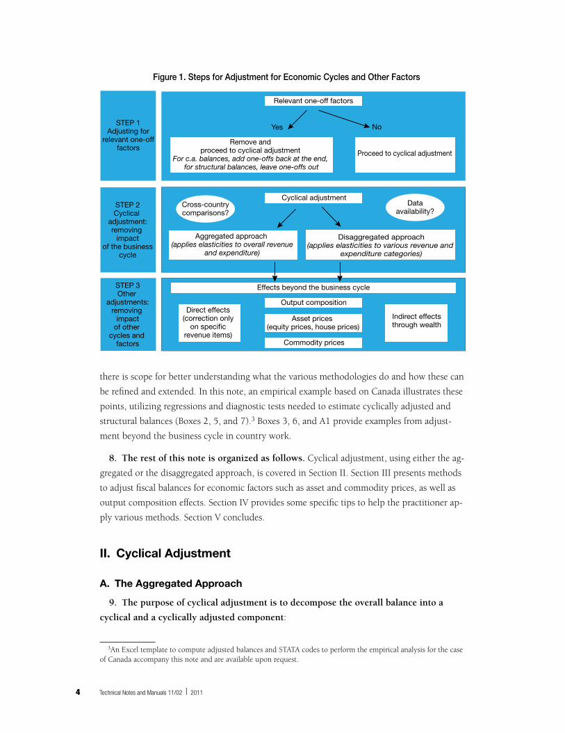
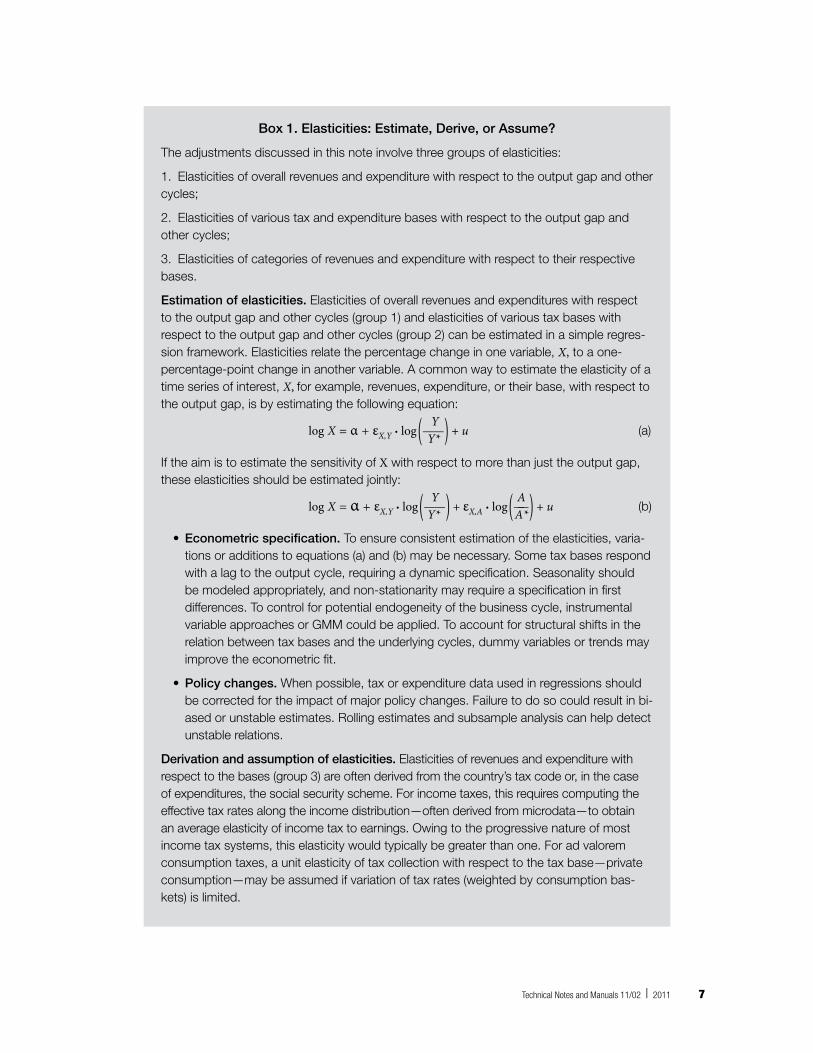
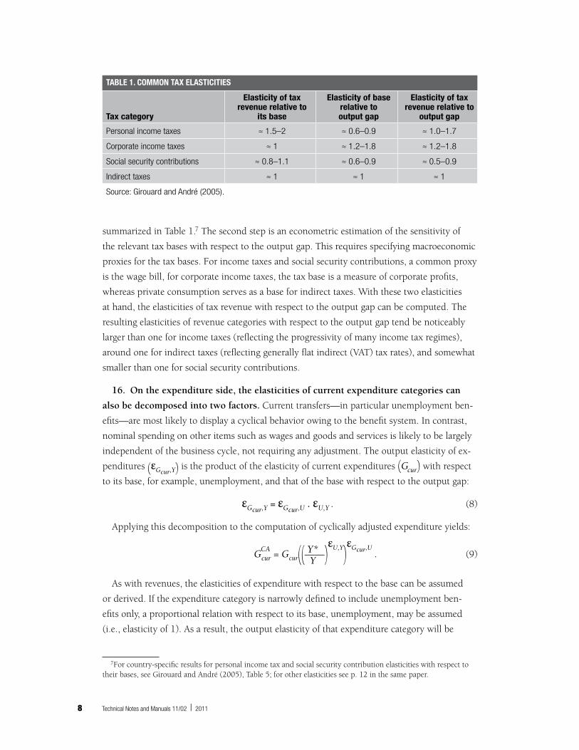
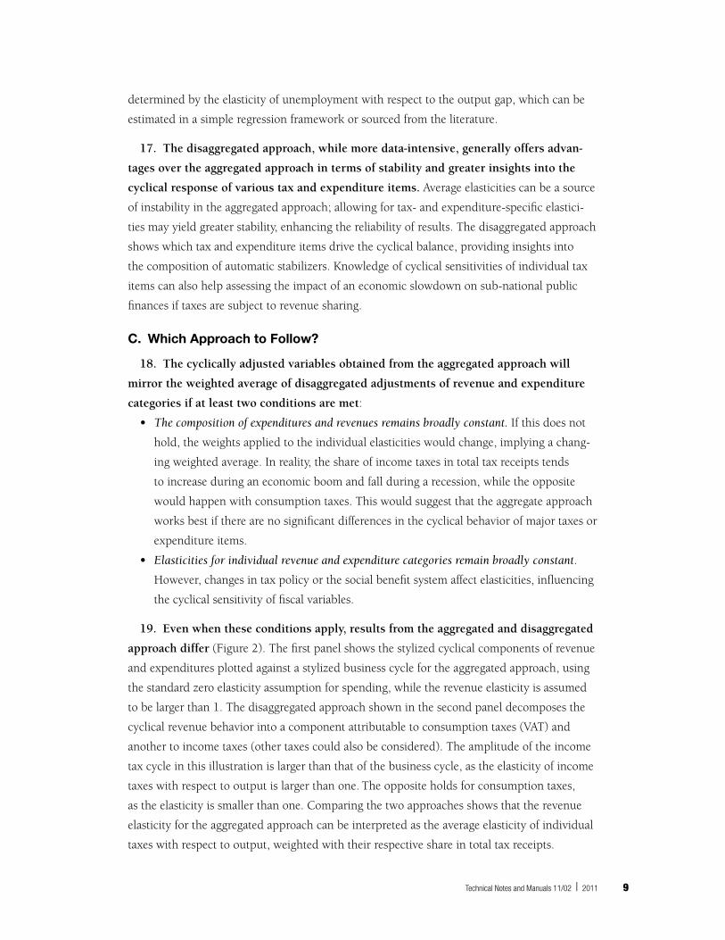
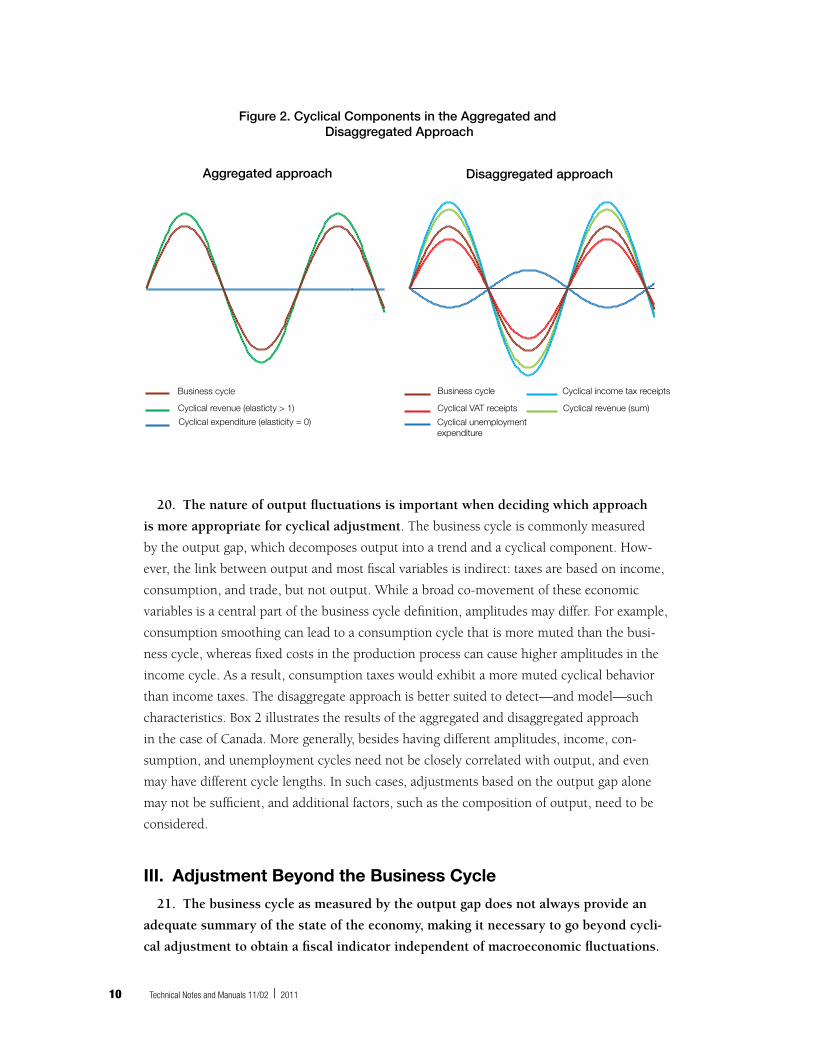
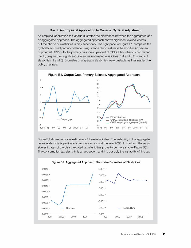
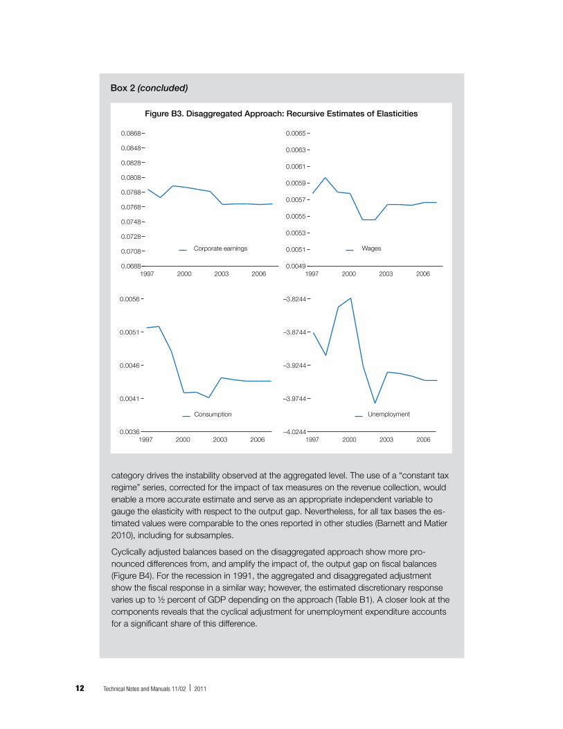
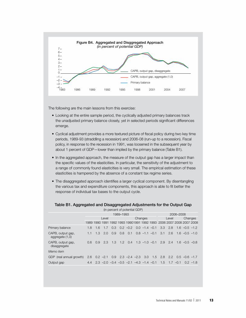
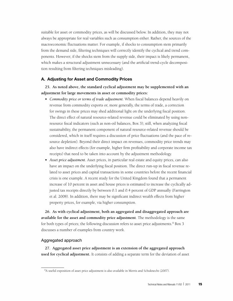
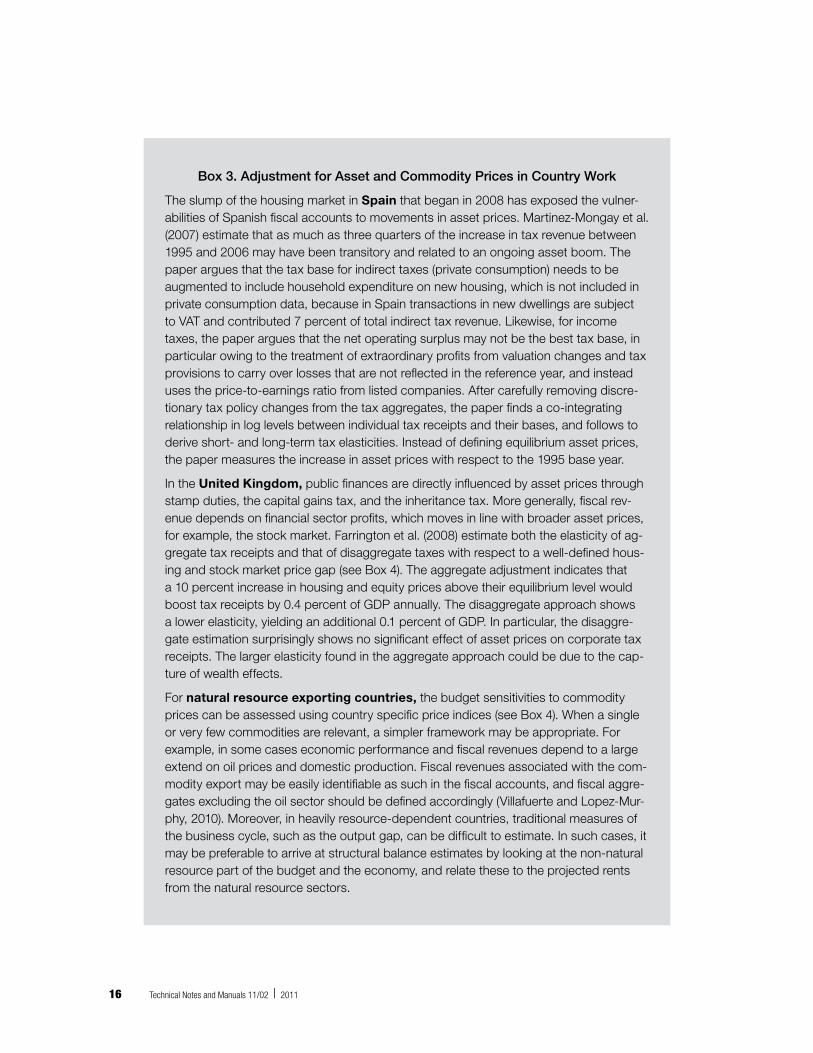
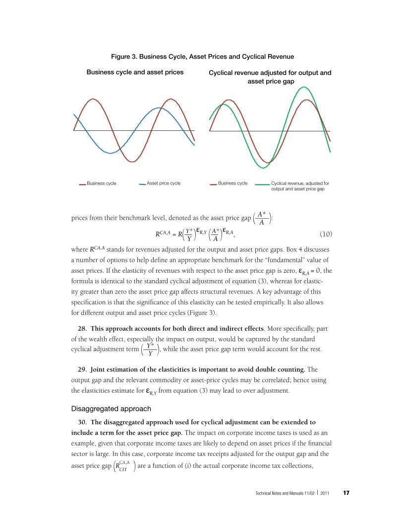
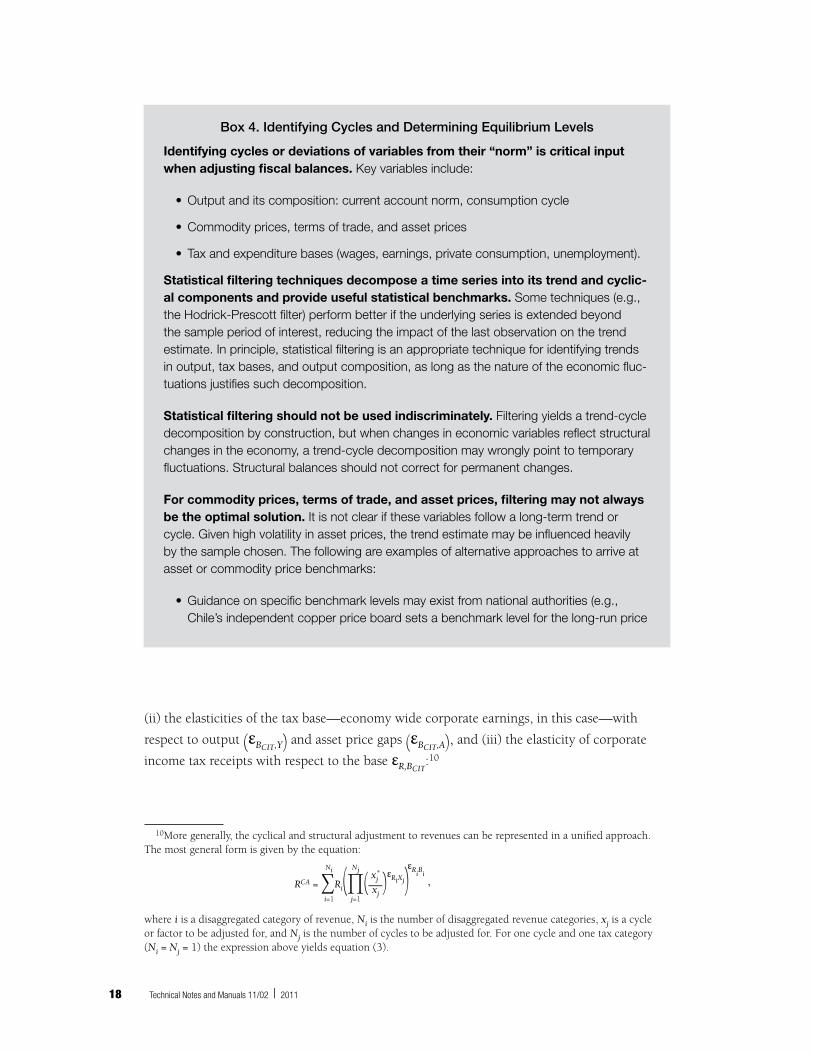
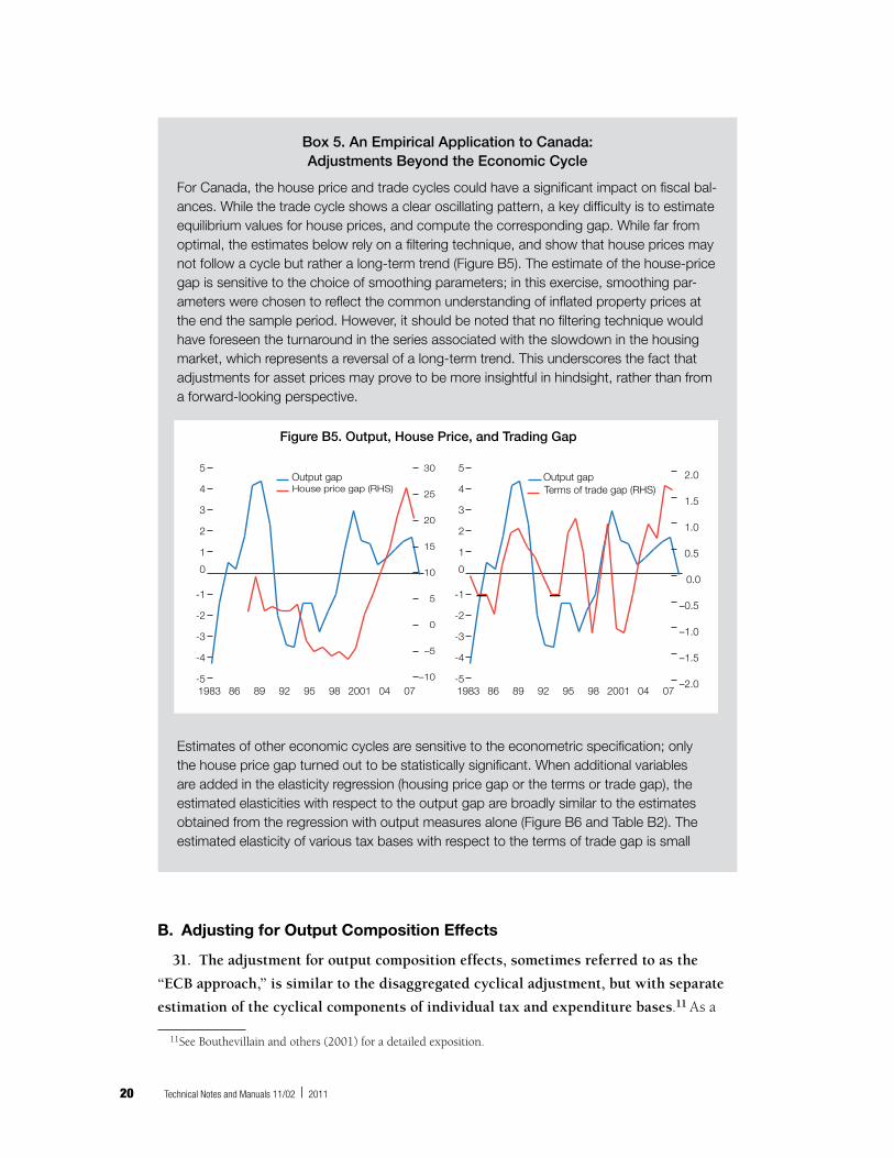
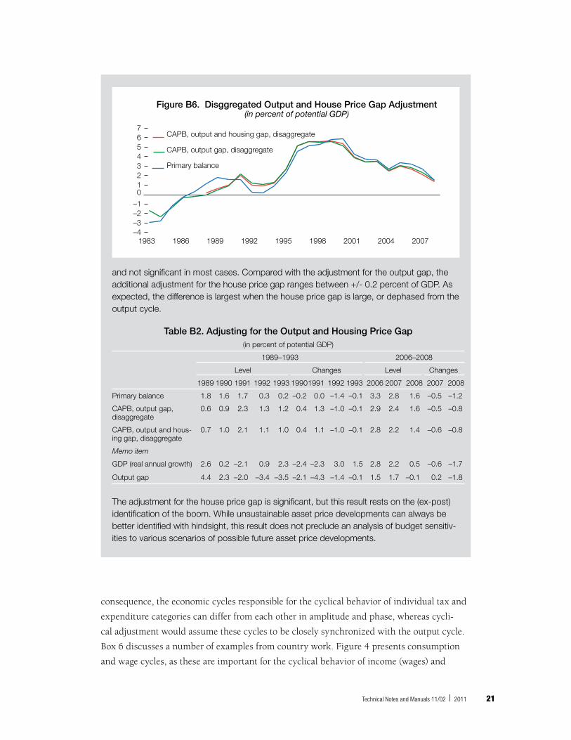
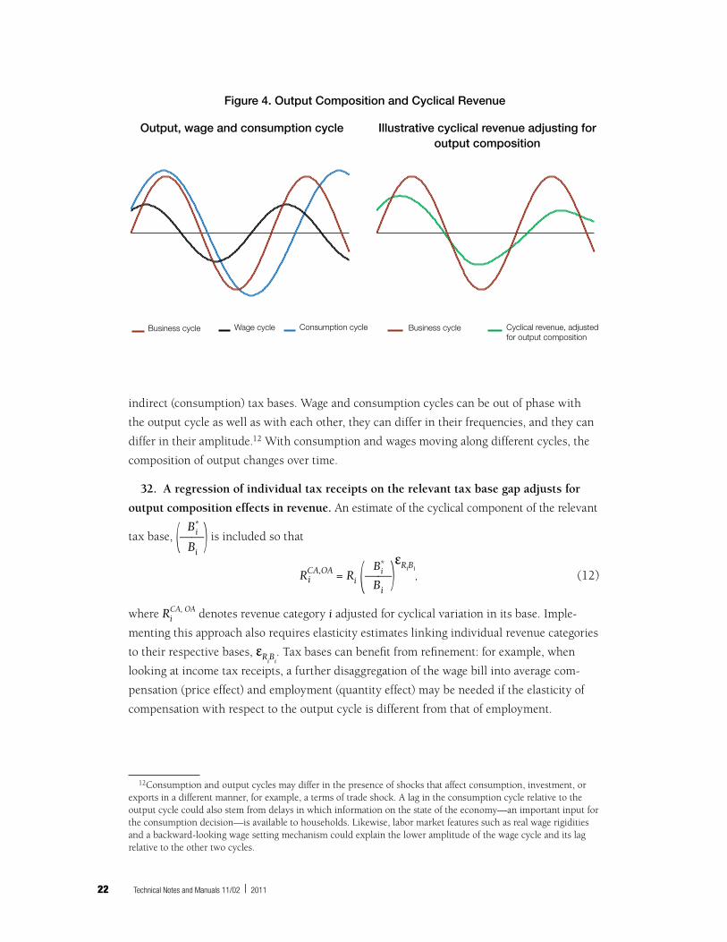
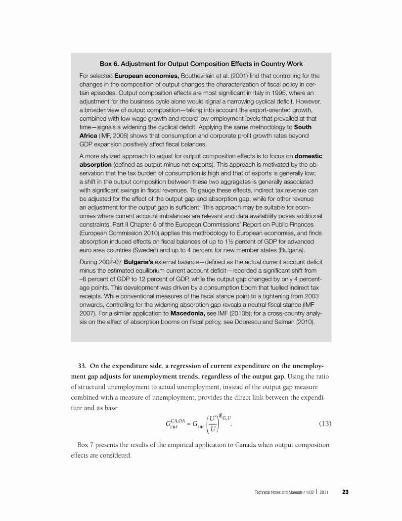
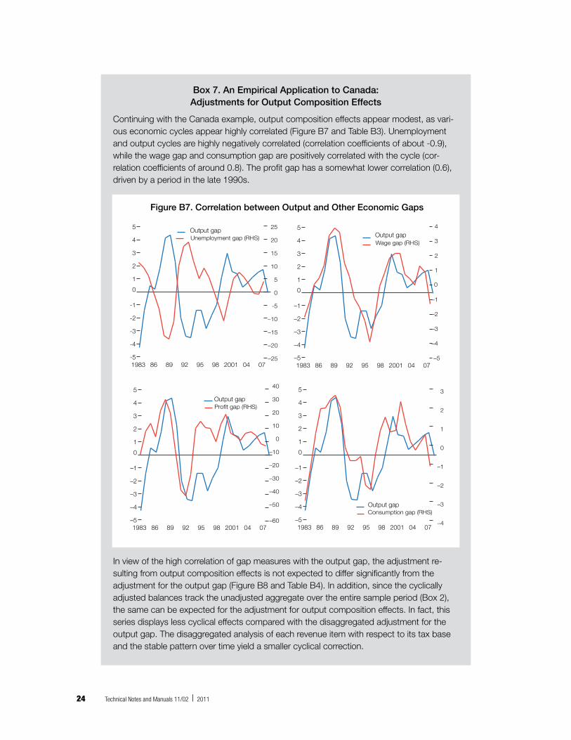
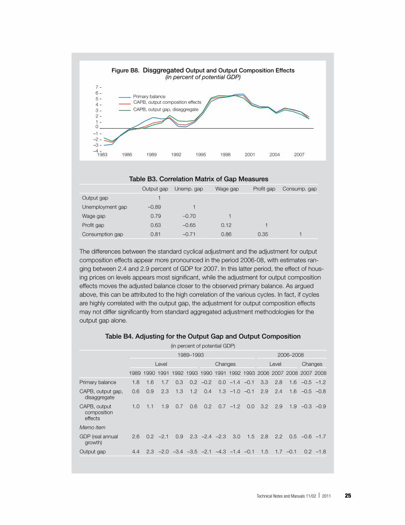

TNM1102
International Monetary FundFiscal Affairs Department700 19th Street NWWashington DC 20431USATel 1-202-623-8554Fax 1-202-623-6073