When and How Should Firms Differentiate? Quality,Advertising and Pricing Decisions in a Duopoly

Dominique Olié Lauga, Elie Ofek, and Zsolt Katona∗

November 28, 2018

∗Dominique Lauga is a University Senior Lecturer in Marketing at the University of Cambridge JudgeBusiness School, d.lauga@jbs.cam.ac.uk, Tel.: +44 1223 768 495. Elie Ofek is the T.J. Dermot Dunphy

Professor of Business Administration at the Harvard Business School, eofek@hbs.edu, Tel.: +1 617 495 6301.

Zsolt Katona is the Cheryl and Christian Valentine Associate Professor at the UC Berkeley, Haas School of

Business, Tel.: +1 510 643 1426. The authors thank Miklos Sarvary, David Soberman, Timothy Van-Zandt,

participants of the marketing track at the INFORMS Annual Meeting, CJBS marketing camp and the 8th

Workshop on the Economics of Advertising and Marketing, as well as seminar participants at UT Dallas and

London Business School for valuable suggestions.

When and How Should Firms Differentiate?Quality, Advertising and Pricing Decisions in a Duopoly

Abstract

One of the hallmarks of competitive interaction is each firm’s desire to differentiate from rivals.

Although differentiation may be achieved through product related choices, advertising levels may

constitute another key mechanism. In this paper, we examine under what conditions firms will

elect to differentiate through product quality vs. advertising intensity and characterize the set of

equilibria that emerge. Consumers can only purchase from the set of products they are informed

about through advertising, and choose the alternative that maximizes their utility. Firms select

product quality in a first stage, advertising levels in a second stage, and prices in the last stage.

We study two forms of advertising–blanket and targeted. Under blanket advertising, firms com-

municate indiscriminately and a consumer’s probability of seeing an ad depends on the level of ad

expenditure. We find that when advertising is ineffective, i.e., the additional awareness generated

by a heavy level is modest relative to the cost, both firms choose a light ad spending. This allows

them to minimally differentiate in qualities without concern of intense price competition, as each

firm expects to have a segment of ‘captive’ consumers that are only aware of its product. When

advertising is moderately effective, one firm shifts to expending heavily on advertising, hence all

consumers are aware of its product. However, the rival prefers to differentiate by advertising lightly,

while choosing the same maximal quality level. This strategy softens price competition by inducing

the heavy-advertiser to price highly more often in order to capitalize on its captive segment and

allows the light-advertiser to increase its average price. Interestingly, we show that even if advertis-

ing heavily entails no extra cost, one firm will choose to advertise lightly in equilibrium for strategic

reasons. When advertising is very effective, both firms advertise heavily. In this scenario, firms

must differentiate in qualities in order to achieve positive profits. Under targeted advertising, we let

firms choose the segment(s) they wish to inform. We identify conditions such that both firms choose

equally high quality products, but advertise to distinct segments; thereby achieving differentiation

through ad targeting. We further show that this can result in a pocket of unserved consumers,

even though consumers with lower willingness to pay purchase. Generally speaking, we show that

allowing market awareness to be determined endogenously suggests far less product differentiation

than previously suspected and reveals regions where advertising creates viable differentiation.

(Product Quality, Advertising, Differentiation, Pricing, Competition)

1 Introduction

In most markets, firms must figure out how to contend with competitors. The presence of rivals

means that consumers have multiple offerings to choose from, and hence demand for each company

is by no means guaranteed. As they seek to navigate this challenge, firms typically consider ways

to set themselves apart from the competition in order to avoid a “race to the bottom” in prices that

would erode any and all profits. A common approach to softening such detrimental competitive

intensity is through product positioning. In particular, vertical product differentiation may help

avoid the dreaded “head to head” battle with rivals and allow each firm to carve out its own demand

in the marketplace. Several examples of such a strategy come to mind. In the hybrid-electric vehicle

market between 2003-2013, for instance, Toyota’s Prius had several advantages over other hybrids,

such as the Honda Civic hybrid (e.g., in miles per gallon, battery life, and handling).1 And, as

assessed by Consumer Reports (on a 100-point scale), a host of categories such as vacuum cleaners,

oven ranges, laptops and fitness trackers, exhibit a substantial amount of quality variation between

high- and low-end models (see top panel of Table 1).

However, causal empiricism suggests that there are also numerous industry contexts in which

firms’ products are quite similar in quality and yet they are able to achieve positive profits. Cordless

drills are one such instance where several brands, such as Makita, DeWalt and Milwaukee, offer

products with similar specs.2 Furthermore, as assessed by Consumer Reports, categories such as

lawn mowers, snow blowers, washers, and dryers seem to exhibit a relatively small degree of quality

dispersion across models (see bottom panel of Table 1). Thus, it is likely the case that these firms

are withstanding competitive pressures by “differentiating” through other strategic choices, despite

having the option of selecting dissimilar qualities.

Two prominent actions, aside from product, that firms have at their disposal are advertising

and pricing. The former is presumably intended to help firms communicate their offering, while

the latter affects the value they can extract from customers (vs. leaving more of the value created

with customers). Yet as with product, here too one observes a range of behaviors. Specifically,

some markets are characterized by firms selecting similar levels of advertising, whereas other mar-

1See, for example, Reynolds, “Hybrid Sedan Comparison: 2006 Honda Civic Hybrid vs. 2006 Toyota Prius,” in

MotorTrend, August 11, 2006; and Edmunds (https://www.edmunds.com/toyota/prius/2005/comparison-test.html).2For example, review website justcordlessreviews.com gives these three brands similar ratings of 4.8, 4.7, 4.9,

respectively (accessed June 2018).

1

Table 1: Quality and Price Dispersion for Select Categories (Based on Consumer Reports, 2017)

Large Quality

Dispersion

ProductAverage Quality

StandardDev.

Quality

Average Price

StandardDev. Price

Computers, Laptop: 10- to 11-inch 55.4 13.3 $385 290.3

Ranges: gas and dual-fuel, single oven (30") 58.9 12.6 $1,437 788.7

Computers, Laptop: 11- to 15-inch 68.8 11.6 $843 318.7

Ranges: smoothtop, double oven (30") 72.8 10.7 $1,658 428.6

Dishwashers 70.4 9.7 $854 407.3

Fitness Trackers: built-in data readout 72.6 9.6 $153 56.3

Vacuum Cleaners: bagless upright 51.9 9.3 $215 112.8

Small Quality

Dispersion

Snow Blowers: two-stage gas 87.1 3.8 $1,235 266.7

Generators: large stationary 90.75 3.3 $3,950 1618.5

Dryers: gas 78 2.7 $1,127 227.9

Dryers: electric 78.1 2.6 $1,044 241.8

Washers: front loaders 82.7 1.5 $1,134 287.4

Lawn Mowers: gas, self-propel 21.2 1.2 $298 36.6

Lawn Mowers: battery-powered 19.5 0.7 $425 47.2

kets exhibit asymmetric levels across firms. For example, home improvement retailers Home Depot

and Lowe’s spent similar amounts on advertising in 2017, while major wireless carriers spent very

different amounts (see Table 2 for these and other examples). Moreover, there can be consider-

able heterogeneity between industries in terms of the ball park level of advertising spending. For

instance, the automotive industry expends the most on measured media ads (over $17 billion in

2017), while the household supplies category only spends about a third as much.3

Likewise with pricing, in some categories one observes fairly stable prices over time while in

others frequent price promotions are common (Mohammed 2011). There can also be variations

within industry— as several department store retailers tend to play every day low pricing (or EDLP)

and offer discounts over a small range of prices (e.g., Walmart), while others tend to offer more

frequent and variable price promotions (or Hi-Lo pricing, e.g., Kohl’s); and some computer makers

3See Statista Dossier on Automobile Advertising in the US (2017) and Standard Media Index,

www.standardmediavillage.com (also reported in eMarketer, “Top 10 US Industries, Ranked by Ad Spending,” 2018).

A survey of CMOs also points to heterogeneity in spending when one looks at the percent of revenue budgeted to

marketing (anywhere from 2.4% to 18.9%; The CMO Survey and Deloitte Digital, 2018, www.cmosurvey.org).

2

are well known for maintaining price consistency and seldom discount (e.g., Apple, see Stuart

2011), whereas other players tend to cut prices frequently and deeply (e.g., Lenovo).

Table 2: Advertising Spending in 2017 in Select Categories*

Category CompanyTotal U.S.

advertising spend (millions of $)

Home Improvement RetailHome Depot 911

Lowe’s 893

Cruise Lines Norwegian Cruise Lines 223

Royal Caribbean Cruises 213

Wireless Carriers

AT&T 3,520

Verizon 2,643

T-Mobile 1,800

Sprint 1,300

Insurance

Geico 1,503

Progressive Corp. 911

State Farm Mutual 860

Allstate Corp. 717

Liberty Mutual 451

Nationwide Mutual 283

* Dark-shaded categories exhibit similar ad levels across firms; light-shaded categories exhibit considerable heterogeneity. (Source: AdAge, Leading National Advertisers, June, 2018)

Complicating matters, there is sometimes an observed interaction between product quality and

ad levels, with some studies finding that higher quality firms also advertise more extensively than

lower quality rivals (e.g., Archibald et al. 1983, Tellis and Fornell 1988), while in other cases no such

systematic empirical relationship was found (e.g., Kash and Miller 2009, Caves and Greene 1996).

One must also bear in mind that in some cases firms can be selective in their advertising efforts. For

example, by compiling a list of consumers that meet certain criteria firms can send targeted e-mails

or direct mail, and in B2B settings firms can dispatch their sales force to a subset of potential

customers with common characteristics. Digital advertising (e.g., on Facebook or Instagram) also

provides a number of opportunities to define target segments in detail.4 In other cases, firms cast

4Most social media platforms allow firms to specify certain filters based on a person’s profile, past brows-

3

a much wider net and use media outlets that preclude direct control over who sees their ads. For

example, by running a commercial on national TV (e.g., on the Superbowl) or placing an ad on a

general interest website (e.g., on CNN.com), a firm will potentially reach a broad set of consumers.

Although academics and practitioners have suggested that the nature of communication (targeted

vs. non-targeted) can affect ad spending (Soberman 2005, Eechambadi 1994), no clear distinctions

have been drawn on the role each format can play in withstanding competition vis-à-vis product

quality.

It is not intuitively obvious why such heterogeneity in industry patterns exists and how to

reconcile the variety of strategies along the three decision variables of product quality, advertising,

and price — in effect, three of the so-called marketing “4Ps”. The objective of this paper is to

shed light on these matters and help understand firm behavior by addressing the following research

questions.

• When should we expect firms to differentiate in product qualities and when in advertisinglevels, assuming both strategies are available to them?

• Is it possible for firms to sustain positive profits with undifferentiated levels of quality andadvertising? What pricing approach is needed to enable this outcome?

• If firms can target their advertising efforts, under what conditions should we expect themto select distinct vs. overlapping segments, how does this decision impact their quality and

pricing policies, and what is the nature of the demand structure that arises?

To address these questions we develop a duopoly model in which firms choose product quality

in a first stage, select their advertising levels in a second stage, and set prices in the last stage.

Consumers are heterogeneous with respect to their valuation for quality, yet in order for them to

consider the purchase of a product they must first be aware of its existence and informed about

its characteristics. Although there are several ways consumers can become informed about the

products available in the marketplace, firm initiated communication is a primary vehicle.5

On a given purchase occasion, consumers evaluate the various products they are informed about

ing/purchase behavior, and messages in their feed, that can be used for targeting purposes by advertisers. Similar

filters are also available to advertisers on search engines such as Google.5 In the U.S. alone, companies spent close to $200 billion in 2017 to advertise their offerings to consumers (Adver-

tising Age, “200 Leading National Advertisers 2018,” June 26, 2018).

4

and choose the one that delivers them maximum utility. Consequently, the return on advertising for

a firm will critically depend on how its offering compares to the other alternatives in the marketplace

and on how aggressively those products are advertised. In this context, the decisions of what quality

product to offer and then how heavily to promote it through advertising become intertwined, and

further depend on the resulting pricing the firms pursue. This structure allows us to examine the

research questions laid out above; thereby shedding light on which strategic lever(s) a firm should

pull in an effort to effect differentiation from a rival.

Our analysis looks at two forms of advertising commonly used to inform consumers about

products (for empirical support on the informative role of advertising see, e.g., Ackerberg 2001,

Caves and Greene 1996, Bagwell 2007). The first type–blanket advertising–captures situations

where communication is indiscriminate and the probability that consumers become informed about

the firm’s product is a function of the advertising expenditure level. Specifically, a heavy ad spend

guarantees that all consumers receive the firm’s message and consider its product, while a light ad

spend only results in a likelihood (which is less than 1) that each consumer receives the message.

We find that three equilibria can emerge depending on the effectiveness of advertising, which is

defined as the extra impact on demand that a heavy ad spend has over a light ad spend relative

to the cost of doing so. Specifically, when advertising is ineffective, firms are fully undifferentiated

in their actions: they choose the same product quality, the same advertising level, and the same

pricing strategy. Price competition is softened because through their advertising choices firms

limit the expected number of consumers who will consider both products; hence they earn healthy

profits by co-locating on the highest quality position, leading to minimal product and advertising

differentiation. We further show that by choosing to co-locate in quality in the first stage, a firm

can “prevent” its rival from shifting to the heavy ad spend level in part of this region, even though

a monopolist would already find it profitable to do so to gain from greater consumer awareness.

When advertising is moderately effective, asymmetric advertising choices with no product dif-

ferentiation occurs. Specifically, one firm always has an incentive to choose a high-quality product

and advertise heavily. Interestingly, the rival still finds it optimal to select the same high quality

level, but in order to soften price competition it must advertise lightly (otherwise, if both advertise

heavily and are undifferentiated in the quality space then price competition intensifies and profits

will be driven to zero). In doing so, the light advertiser concedes an entire segment of consumers

to the heavily advertising firm, yet benefits from the higher average equilibrium prices that ensue.

5

We further show that this incentive can be so strong in this region that, even if advertising heavily

entails no extra cost, one firm still prefers to select the same high product quality but differentiate

by refraining from advertising heavily. Finally, when blanket advertising is very effective, in the

sense that the bump in market awareness from advertising heavily is large and comes at relatively

little cost, quality differentiation with no advertising differentiation is the equilibrium outcome. In

this case, a firm cannot afford to advertise lightly because it will then be relinquishing a very large

segment of consumers who will only be aware of its rival’s product. Instead, both firms advertise

heavily with one firm choosing maximal quality and a high price, while the rival differentiates with

a much lower quality product and a cheaper price.

Thus, our findings suggest that with blanket advertising firms tend to utilize at most one of

the actions at their disposal to soften competition — (i) advertising differentiation: selecting the

same product strategy yet using distinct advertising levels to endogenously segment the market in

terms of awareness, or (ii) product differentiation: choosing dissimilar product positions, thereby

leveraging customer heterogeneity in willingness to pay for quality, yet both electing to advertise

heavily. In these instances, pricing strategies are also differentiated. In particular, in case (i) the

heavy advertiser selects higher prices on average than the light advertiser, and in case (ii) the

high-quality firm prices higher than its low-quality rival. No differentiation in product quality

or advertising is feasible as well, as long as the advertising levels chosen are light; in which case

the resulting prices are in similar mixed strategies. We further characterize how equilibrium profits

depend on advertising effectiveness and uncover a non-monotonic pattern: firms’ profits can initially

increase and then decrease, with profits rising again for the firm switching to the heavy advertising

level.

The second type of advertising we examine—targeted advertising–captures situations where

firms can be selective and communicate to specific segment(s) they wish to inform about their

product. With this form of advertising we establish the conditions for a robust equilibrium out-

come whereby advertising strategies are “differentiated”, in the sense that each firm targets its

communication to a distinct segment. Because every consumer considers at most only one prod-

uct, the firms do not directly compete in the pricing stage and hence can both choose equally

high qualities–that is, their products are undifferentiated. Depending on segment sizes, firms may

asymmetrically expend on advertising and it may be the case that the firm targeting the lower

willingness-to-pay segment spends more yet prices below its rival.

6

Surprisingly, there exist conditions such that a set of consumers with moderate valuation for

quality are advertised to but make no purchase, even though consumers in a separate segment

with lower willingness to pay are served. Additionally, one might have expected that as long as

firms choose the same product quality then how the market is split between them should not affect

total demand. However, we show that the total number of consumers served in equilibrium follows

an inverted-U shape as a function of the targeting criterion. Lastly, we discuss the possibility of

an equilibrium in which firms differentiate in product qualities and targeted advertising strategies,

with the high-quality firm covering the entire market and the low-quality firm forgoing the premium

segment.

Collectively, these results uncover when and how firms strategically use product quality, adver-

tising and pricing to effectively compete: in some cases differentiating in the advertising approach

taken, while electing similar product qualities, and in some instances differentiating through qual-

ity divergence, while electing similar advertising approaches. There are also scenarios where both

actions are similar across firms. The range of patterns that can arise in equilibrium, depending

on certain parameter values, may thus help explain the variation observed in practice with respect

to these key decision variables and the seemingly inconsistent empirical research findings on the

connection between product quality and advertising levels.

The rest of the paper is organized as follows. The next section relates our work to the relevant

literature and summarizes our contribution. Section 3 sets up the basics of the model in terms

of demand and firm behavior. Section 4 solves for the case of blanket advertising and Section 5

solves for the case of targeted advertising. Finally, Section 6 offers some managerial and empirical

implications, discusses extensions and limitations, and outlines opportunities for future research.

To enhance readability, we postpone all proofs to the Appendix.

2 Related Literature

Our work is primarily related to two streams of literature, the first pertaining to quality differen-

tiation and the second to the relationship between advertising and product quality.

Within the stream of literature on vertical product differentiation, the widely known model of

Shaked and Sutton (1982) examines price competition between firms that first choose the quality

of the products they sell. Since consumers are assumed to be fully informed about all products in

7

their model, in equilibrium firms choose different qualities in order to reduce price competition in

the last stage.6 Moorthy (1988) relaxes Shaked and Sutton’s zero production cost assumption by

introducing a quadratic cost function for quality. While this can result in an equilibrium where the

firm choosing the lower quality is better off, it is still the case that in any equilibrium (simultaneous

or sequential move) firms differentiate in qualities. Assuming that firms do not cover the market,

Choi and Shin (1992) show that the low quality firm will choose a quality level that is a fixed

proportion of the high quality firm’s choice. Wauthy (1996) gives a full characterization of quality

choices, allowing market coverage to be endogenous. More recently, Choudhary et al. (2005) and

Jing (2006) find that the higher quality firm can be worse off in equilibrium. Choudhary et al.

(2005) allow personalized pricing, which can intensify competition to the detriment of the high

quality firm. Jing (2006) identifies the conditions on the cost structure under which producing the

low-quality good can be more profitable. These studies all show that quality differentiation is a

robust equilibrium outcome.

However, in reality similar quality products are often observed in the marketplace. Rhee (1996)

cites evidence for this and offers an explanation that incorporates consumer heterogeneity along

unobservable attributes into the vertical differentiation model. As a result, if consumers are suffi-

ciently heterogeneous on the extra dimensions, in equilibrium firms offer products that are identical

on the observed quality dimension yet differentiated on the unobserved dimensions. Bester (1998)

investigates the case of experience goods defined along two dimensions: an imperfectly known ver-

tical quality level (that can either be high or low) for which there is no consumer heterogeneity,

and an observable horizontal attribute for which consumers’ tastes are uniformly distributed. His

analysis shows that both firms have an incentive to choose the high quality level and use sufficiently

high prices to signal this choice, which allows them to minimally differentiate along the horizontal

attribute. Banker et al. (1998) investigate the relationship between equilibrium quality levels and

the intensity of competition between firms. They find that the degree of differentiation depends on

the market structure and production cost differences.

Notably, the papers in this stream analyze firms’ quality positions under various price and cost

assumptions, but presume that all consumers consider all the products available. Hence, these

6 It is worth noting that earlier work had identified several of the forces operating in Shaked and Sutton (1982).

Specifically, Gabszewicz and Thisse (1979) build a model with two products of exogenously known quality levels.

They characterize the pricing equilibrium of this game and show that the comparative statics are such that if the

qualities get closer to each other then price is driven to zero, leading them to conclude that: “we have thus natural

forces which lead the duopolists to maintain product differentiation.”

8

works ignore the fact that in many markets consumers are ex-ante uninformed (or need to be

reminded) about the various offerings, with advertising serving as an additional lever firms might

use to differentiate and soften competition.

The second stream of literature related to our work involves studies on the connection between

advertising choices and product positions. It is theoretically well-established in economics and

marketing that advertising levels can signal product quality (Milgrom and Roberts 1986); although

little empirical evidence exists to conclusively support this idea (Bagwell 2007, and references

therein). Such works ignore advertising’s role in informing consumers about which products exist

(Nelson 1974, Butters 1977) and thus its effect on market size. Grossman and Shapiro (1984) model

advertising as informative in a horizontal set up, whereby receiving an ad increases the probability

a consumer finds a product that better matches his or her tastes. They find that firms select

excessive advertising levels relative to a social planner and that more efficient advertising technology

intensifies price competition. Iyer et al. (2005) investigate targeted advertising when consumers have

horizontal tastes and find that firms advertise more often to consumers who have a strong preference

for their product, arguing that this is a way to soften price competition and eliminate wasted

advertising. Other papers (Chen et al. 2001, Zhang and Katona 2012) examine how individual

targetability or targeting accuracy affects competition, showing that imperfect targetability can

reduce competition by serving as an implicit differentiator. While some of these forces will be

relevant in our context, much of the literature studying targeting aspects of advertising, such as

the paper by Narasimhan (1988), treats qualities as given. By contrast, we add quality as an

important decision variable and show that endogenizing both product quality and advertising level

critically affects equilibrium outcomes.7

Our paper also contributes to the debate on whether higher quality products should be as-

sociated with higher levels of advertising and prices, with the empirical literature finding mixed

evidence for such a relationship (Erdem et al. 2008, Kash and Miller 2009, Caves and Greene 1996,

7 In Zhu and Dukes (2017), firms need to decide which product attribute(s) to make prominent (e.g., through

advertising) when consumers have limited attention and heterogeneous horizontal tastes. They show that firms may

choose to make the same attribute prominent and that this can impact endogenous quality choices. Our setup is

different: we assume only one attribute and a firm’s communication level affects the fraction of consumers aware of

its product, independently of its rival’s advertising efforts (in Section 6.2 we briefly discuss communication spillover

effects, which is a characteristic of the modeling in Zhu and Dukes 2017). We note that Varian (1980) assumes the

exogenous existence of two customer segments: uninformed and informed. Firms are undifferentiated in his model,

hence they compete using mixed pricing strategies. Our paper can be interpreted as extending his work by allowing

firms to select product qualities and endogenously create informed and uninformed segments.

9

Archibald et al. 1983, Tellis and Fornell 1988, Song et al. 2016). Our analysis can help reconcile

these seemingly inconsistent observations by delineating conditions for when a positive relationship

should hold between these actions and when it should not in equilibrium.

In summary, our contribution lies in extending the first stream of literature by exploring the

strategic role of advertising as another action, in addition to product quality, that firms can take

to withstand competitive pressures. We characterize when and how firms use each of these two

actions to differentiate and uncover important interactions between the two variables. Relative

to the second stream, we endogenize product qualities and analyze how this decision is impacted

by foreseeing the need to advertise to inform consumers and by the ensuing pricing equilibrium

that can be in mixed or pure strategies. We further show that, given the opportunity to use

targeted advertising, firms may minimally differentiate in qualities. That is, if consumers are

initially uninformed about products, there is no need to divide the market by choosing distinct

quality positions, since a division is created by the targeted advertising choices.

3 Model Setup

We consider two competing firms that seek to sell a product in a given market. We index the firms

by the numbers 1 and 2 or the letters and , always assuming that 6= . If firms offer different

quality products, we denote the firm offering the lower quality product by 1 and the one offering

the higher quality product by 2. We assume that every consumer purchases at most one unit. We

further assume that consumers are heterogeneous with respect to their valuation of quality, denoted

by . The parameter is uniformly distributed in the interval [0 1]. A consumer with parameter

gains utility − from a product with quality priced at , and purchases the product for

which his/her utility is greater (provided the net utility is non-negative). However, consumers can

only purchase products they are informed about (Keller and Kotler 2011). By advertising, a firm

communicates the existence and characteristics of its product, thereby affecting the likelihood that

it enters a consumer’s consideration set. Our setup is thus consistent with the informative view of

advertising (see, e.g., Tirole 1988, Bagwell 2007) and with consumer behavior research (e.g., Mitra

and Lynch 1995).8

8Trivially, an individual cannot consider buying a product that s/he is not aware of. Yet the consideration set

can be narrower than the set of products the consumer is aware of, since some alternatives may be excluded before

carefully comparing the utilities derived from them (Hauser and Wernerfelt 1990). Because informative advertising

impacts the salience of products and their characteristics in consumers’ memory, it affects which products are “top

10

We study two types of informative advertising mechanisms. In the first type, which we call

blanket advertising, the probability that a consumer is informed about firm ’s product is , inde-

pendently for each consumer. This probability depends on how intensely firm advertises and is

uncorrelated with firm ’s advertising level. In the second type, which we call targeted advertising,

firms can communicate to subsets of consumers that belong to distinct segments. If a consumer

is in a firm’s targeted segment, s/he is informed about that firm’s product with probability 1. In

Section 6.2, we discuss our modeling assumptions on advertising and mention possible extensions

(such as persuasive and spillover effects), as well as comment on additional ways consumers can

learn about products (e.g., through search).

Timing : The timing of the game is as follows. First, firms choose their qualities (without

loss of generality 1 ≤ 2). Qualities are positive and have a maximum value that is normalized

to 1. Second, firms make their advertising decisions. In the blanket case they set their advertising

level and in the targeted case they choose the segment(s) they wish to advertise to. Third, firms set

prices. Finally, consumers make their purchase decisions. This timing reflects the notion that the

quality position choice tends to be a long-term decision, whereas prices can be easily changed. The

time-scope of advertising decisions is somewhere in between. It is further common for advertising

allocation decisions to come after product positioning has been determined but before prices are

set (this timing assumption is consistent with several prior works, e.g., McAfee 1994, Roy 2000). In

practice, while prices can be adjusted on a weekly, daily or even hourly basis, advertising budgets

and media planning are typically set on a quarterly or annual basis.9

Costs and Profits: We assume no fixed entry costs, hence both firms participate in the market.

Furthermore, we assume that variable production costs are constant and normalize them to zero.10

of mind” at the time of purchase. Hence, our model applies even if we assume that consumers are generally aware

of all products. All we require for our results to go through is that advertising sufficiently increases the likelihood

of a product entering the consumer’s consideration set. This can also be seen as consistent with the repeat-business

effect of advertising (Nelson 1974). Iyer et al. (2005) have a similar interpretation in this regard.9 It is important to note that our modeling and timing structure do not preclude the possibility that a firm

may include price (or some discount/sale promotion) in a particular ad execution. The idea is that the amount of

advertising and likely even the media buy intentions have been set prior to final prices being decided upon (and these

final prices can later appear as part of the ad copy). In other words, the specific content of ads may be changed more

easily than the decision on whether an aggressive or unaggressive approach to advertising will be taken. Our modeling

is also consistent with papers that assume consumers can costlessly obtain information on price after observing an

ad (see, e.g., Mayzlin and Shin 2011).10Normalizing variable costs of production to zero might seem as an oversimplifying assumption but is done for

several reasons. First, it allows us to focus on the strategic incentives to differentiate in qualities when advertising

11

However, advertising costs, denoted (·), depend on the level chosen in the following way. In theblanket advertising case, we assume that () is a non-decreasing function of , i.e., to achieve a

higher likelihood of being considered by a consumer a firm has to spend more on advertising (we

also examine the special case whereby a heavy ad level comes at no additional cost). In the targeted

advertising scenario, we assume that the cost is a linear function of the segment size. Firms’ profits

are therefore simply their revenues (price × quantity sold) minus advertising costs:

Π = − ()

We solve for the sub-game perfect equilibria of the game. We focus on pure strategies for quality

and advertising decisions, yet allow pure or mixed strategies for prices (reflecting the fact that in

several markets firms tend to run occasional price promotions). Next, we characterize the equilibria

in the two advertising cases: blanket and targeted.

4 Blanket Advertising

In this setup, firms communicate to the entire mass of consumers but the probability of a firm’s ad

reaching (or being attended to by) a particular consumer depends on the advertising level it selects.

For the sake of simplicity, let us assume that there are two levels of advertising: light ( = ) and

heavy (), with costs ≤ , respectively. The probabilities of being considered by consumers

are then 0 = . Without loss of generality we set = 1 That is, a firm can either

choose to heavily advertise at a high cost, thereby ensuring every consumer is informed about its

product, or to advertise lightly at a low cost, thus expecting only a portion of consumers to be

informed. We use the notation ∆ ≡ − for the cost differential and ∆ ≡ − for the

ad-impact differential between the two levels of advertising. We further assume that the ad-impact

differential is not negligible, to ensure that firms don’t trivially always advertise lightly. Formally,

this means ∆ .11

is another option to differentiate. Including production costs would complicate this analysis without providing much

added insights into the questions of interest, as our results should hold over a certain range of cost parameters.

Second, these assumptions correspond to Shaked and Sutton (1982), thus allowing us to directly compare our results

to theirs. Third, the extant literature has examined the implications of incorporating quality-dependent production

costs, with the general finding that as these costs increase firms tend to choose lower qualities (e.g., Jing 2006).

Fourth, for a growing number of goods (such as digital products) variable costs are insignificant regardless of quality.11One way to interpret the lower bound on ∆ (∼0.13) is that there are always some consumers who require

more active communication initiated by the firms to be informed. Note further that if ∆ = 0 (i.e., = 1), byadvertising lightly firms already ensure all consumers are informed about their products. In such a case, advertising

decisions would no longer be a relevant action in creating differentiation and this would trivially correspond to the

full awareness case assumed in prior work.

12

Once firms have advertised their products, consumers may not all have the same consideration

set. Some consumers will be able to consider both products, and they constitute what we call the

competitive segment. We also refer to consumers in this segment as comparison shoppers since they

are able to compare both products (on quality and price) before making their purchase decision.

The size of the competitive segment is endogenous and can be as small as 2 when both firms

advertise lightly or as large as 1 (i.e., the entire market) when both firms advertise heavily. In

addition to the competitive segment, a firm might have what we call a captive segment, composed

of consumers who only consider its product and not the competitor’s. The sizes of captive segments

are also endogenous and depend on firms’ advertising levels, as summarized in Table 3. As can

be seen from the table, only when a firm faces a rival that advertises lightly will it have a captive

segment of its own. For completeness, we note that when both firms advertise lightly there exists

another segment of consumers who are unaware of any offerings (of expected size (1− )2).

Table 3: Existence and Expected Size of Captive Segments as a Function of Advertising Decisions

Ad LevelHeavy ( = 1) Light ( = )

Heavy ( = 1) No captive segmentOnly Firm has a captive

segment of size 1−

Light ( = )Only Firm has a captive

segment of size 1−

Both firms have captive

segments each of size (1− )

A firm with a captive segment always has the option of focusing on these consumers and not

competing for the comparison shoppers. In that case, the firm would act as a monopolist over its

captive segment. Thus, as a benchmark, we first solve the monopolist case, i.e., when there is only

one firm in the market.

A consumer who receives an ad for the monopolist’s product buys it if and only if − ≥ 0.That is, the monopolist’s demand consists of consumers who are informed about the product

and who value quality sufficiently, satisfying the following condition: ≥ . Therefore, the

monopolist’s demand is:

= (1− )

where ∈ { 1}. Given and , the monopolist chooses a price ∗ = 2 to maximize its

13

revenue: (1− ). Its profit becomes

Π = 4− ()

which is increasing in regardless of the advertising level. Hence the monopolist always sets

∗ = 1 in the first stage, and chooses = 1 in the second stage if and only if (4 − )

(14 − ) or ∆ ∆4 . Specifically, the monopolist advertises heavily rather than lightly if the

extra revenue that results from this advertising level is greater than the additional cost∆. Another

way to characterize this decision is in terms of ad effectiveness, measured by the ratio ∆∆ (for

∆ 0). A larger ratio means a greater ‘bang-for-the-buck’, and the monopolist advertises heavily

if the ratio is greater than = 4. Consequently, in analyzing the duopoly case, if a firm chooses

to advertise lightly when ad effectiveness is larger than then we are assured that this is a result

of the strategic interaction between the firms.

Duopoly

Let us now turn to the duopoly case. We seek to understand under what conditions a firm will elect

to use advertising vs. product quality to soften competition with its rival; also allowing for the

possibility of no differentiation on these decision variables. We start by analyzing the advertising

level firms choose in the event they have elected to co-locate on quality in the first stage, followed

by an analysis of quality choice incentives. The next lemma provides the profits to each firm as a

function of advertising choices when there is no product quality differentiation.

Lemma 1 Under no product differentiation (1 = 2 = ), the profits of firm as a function of its

advertising level () and its competitor’s advertising level () are:

Ad Level Heavy ( = ) Light ( = )

Heavy ( = ) = − = (1− ) 4 −

Light ( = ) = (1− ) 4 −

Before discussing the profits revealed in Lemma 1 in more detail, we introduce some notation.

Let (), (), () and () denote the advertising strategies, whereby the first argument

is the advertising level chosen by Firm 1 and the second is the level chosen by Firm 2. We also

refer to Table 3 for the size of the captive segments for the different advertising levels. Turning

14

to Lemma 1, the () case is straightforward: intense price competition is triggered by the lack

of any kind of differentiation. Specifically, when every consumer is informed about both products

that are of equal quality, the market is comprised of only a competitive segment and firms undercut

each other in price. Profits are negative as firms still incur the cost of choosing the heavy ad level.

Next consider the scenario where firm advertises lightly ( = ), and either has no captive

segment (when = ) or a small captive segment of size (1 − ) (when = ). If Firm

chooses a given price with probability one, two scenarios could unfold: (i) if Firm ’s price is high,

its rival is prompted to undercut it slightly to sell to all the comparison shoppers; but then Firm

would want to deviate and undercut its rival’s price, thus triggering a “race to the bottom” to sell

to the competitive segment, (ii) if Firm ’s price is very low, its rival would concede the comparison

shoppers and focus on its own captive segment. But then Firm would have an incentive to deviate

and sell at a higher price (just below Firm ’s price). In either case, Firm cannot choose a single

price in equilibrium and hence plays a mixed pricing strategy. The best response for Firm is

also to play a mixed pricing strategy. Firm competes for the comparison shoppers by trading off

choosing a high price but having a low probability of selling vs. choosing a low price and earning

less per customer yet having a high probability of selling by undercutting its competitor. In the

end, Firm has to be indifferent between all the possible prices in equilibrium, and its profit is

equal to the monopolist rents from selling to a segment of size (1− ).12

The last scenario to discuss is when Firm advertises heavily but its rival does not (). The

size of the captive segment for Firm is now (1 − ) and is relatively large, such that it might

be profitable to sometimes focus exclusively on that segment to extract monopolist rents. Indeed,

with probability (1 − ) firm sets its monopolist price and only sells to its captive customers.

With remaining probability and similar to the situation in the light advertising case, Firm

competes over the competitive segment facing the following tradeoff: choose a high price but have

a low probability of selling or choose a low price and have a high probability of selling but earning

less revenues per customer. In the end, Firm has to be indifferent between all the prices it mixes

over, and profits are thus equal to the monopoly rents over its captive segment.

One conclusion worth highlighting from Lemma 1 is that when a firm advertises lightly it earns

the same profit of (1 − ) 4 − regardless of the advertising choice of its rival. This property

12The details of the distributions from which equilibrium prices are drawn are given in the Appendix.

15

implies that the low-quality Firm 1 can always consider a deviation to co-locate its product with

the higher-quality Firm 2 (resulting in no quality differentiation) and choose to advertise lightly.

Since a profitable deviation should not exist in equilibrium, the profit of Firm 1 has to be at least

as high as the profit from this potential deviation. In other words,

∗1 ≥ (1− )24−

Another conclusion arising from Lemma 1 is that firms with undifferentiated product qualities

can still sustain positive profits by strategically selecting their advertising intensity levels. Indeed,

by choosing a light advertising level a firm strategically lets its rival have a captive segment, which

softens the ensuing price competition because not all consumers will be aware of both products.

With these insights in hand, we can discuss the implications of Lemma 1 for the best response

advertising choices when product qualities are undifferentiated. In the () case, as noted, full

awareness in conjunction with identical products triggers intense price competition that drives

product market profits to zero; yet both firms still incur the cost of advertising heavily. Thus, with

undifferentiated product qualities, Firm is always better off advertising lightly if it expects its

rival to advertise heavily. However, if its rival advertises lightly, Firm needs to compare the profits

from advertising heavily and ensuring that all consumers are aware of its product vs. advertising

lightly and reducing the number of consumers aware of both products (i.e., shrinking the size of the

competitive segment). Lemma 1 reveals that when (1−) 4− ≥ (1−) 4− or ∆ ≤ (∆)2 4 advertising heavily is profitable. In other words, when the ad-impact differential ∆ = 1− and

the quality level are high enough relative to the cost differential ∆, firm will prefer to advertise

heavily when its rival advertises lightly.

To summarize, if firms do not differentiate in product qualities, whether they would elect to

differentiate in advertising strategies (one spending lightly and the other heavily) depends on the ad-

impact differential ∆ relative to cost differential ∆, i.e., on the degree of advertising effectiveness.

Advertising can be considered ‘ineffective’ when selecting the heavy level only provides a small

awareness lift over selecting the light level or when doing so comes at a very costly expense.

Advertising is considered ‘effective’ when the reverse is true.

We now turn to characterizing the equilibrium of the entire game by solving for the subgame

perfect ad levels chosen in the second stage and the quality positions chosen in the first stage. We

start by presenting the typical case where advertising heavily is more costly than advertising lightly

16

Figure 1: Equilibrium Strategies and Differentiation Type as a Function of Advertising Effectiveness

None Advertising Product

Qualities:

Ad Levels:

Prices:

Note: piave is firm i’s average price in the mixed strategy equilibrium. The advertising cost differential is positive.

s1 = s2 = 1

a1 = a2 = L

Same mixed strategy(p1ave = p2ave)

s1 = s2 = 1

a1 = L, a2 = H

Different mixed strategies(p1ave < p2ave)

s1 < s2

a1 = a2 = H

Different pure strategies(p1 < p2)

Ad Effectiveness

em

Differentiation:

(∆ 0) and address the no cost differential case (∆ = 0) in a subsequent Corollary. Formal

details of the cutoff values in each region of the proposition are given in the Appendix.

Proposition 1 When advertising heavily entails some extra cost (∆ 0), the type of differenti-

ation arising in equilibrium is as follows:

1. When advertising effectiveness is low, both firms choose maximal quality coupled with adver-

tising lightly: no product or advertising differentiation.

2. When advertising effectiveness is intermediate, both firms choose maximal quality with one

firm advertising heavily while the other advertising lightly: only advertising differentiation.

3. When advertising effectiveness is high, firms choose distinct quality levels with both advertising

heavily: only product differentiation.

The proposition uncovers an interesting general finding: firms never elect to concurrently differ-

entiate both in product qualities and in advertising levels. It is optimal to either only differentiate

in advertising levels or in product qualities, or to choose no differentiation in these decision vari-

ables. Graphically, Figure 1 illustrates the type of differentiation (in advertising, product quality,

or none), along with equilibrium pricing strategies, as a function of ad effectiveness.

We now discuss the intuition behind the results in Proposition 1, starting from the ineffective

advertising case, i.e., part 1 of the proposition (the left-most region marked ‘None’ in Figure 1).

When selecting maximal product quality in this region, firms anticipate that a light ad spend by

both will lead to the emergence of sizable captive segments. Light advertising levels can thus act

17

to mitigate price competition by, in essence, creating segments that possess distinct information

sets. The mixed pricing strategies played result in each firm primarily catering to its endogenous

captive segment and earning monopoly rents from these consumers. Alternatively, conditional on

Firm 2 selecting the highest quality level and advertising lightly, Firm 1 could elect to differentiate

in quality. This differentiation strategy turns out to be less profitable because it entails selling a

product of lower quality at a much lower price and not realizing the full amount of profits from

the captive segment. Conversely, Firm 2 might like to advertise heavily. But by selecting minimal

product differentiation in the first stage, Firm 1 prevents this from occurring by making this an

unprofitable move; thus inducing Firm 2 to advertise lightly. Notably, throughout this region of

low ad effectiveness the firms are fully undifferentiated — they select the exact same quality level,

the same advertising level, and play the same mixed pricing strategy.13

Recall that when advertising effectiveness is less than a monopolist would choose to advertise

lightly, and when it is greater than it would advertise heavily (this threshold is marked with a

vertical dashed line labeled ‘’ in Figure 1). Naturally, if a monopolist does not want to invest

heavily in advertising, firms in a duopoly would not either. Yet Proposition 1 identifies a region

where both firms select a light ad spend even where a monopolist would already shift to advertising

heavily (the region to the right of the dashed vertical line and to the left of the first bold vertical

line in Figure 1). This happens because the minimal product differentiation strategy embraced in

the first stage lowers the benefits of advertising heavily, and prevents each firm from switching to

this level even though a monopolist would.

As advertising becomes more effective (Proposition 1 part 2, the middle region marked ‘Ad-

vertising’ in Figure 1), one firm has an incentive to advertise heavily; thereby ensuring the entire

market is aware of its offering and incurring the cost of doing so. If Firm 1 expects its rival to

select the top quality (2 = 1) followed by heavy advertising, what are its optimal product and

advertising strategies? Firm 1 can either co-locate on quality and advertise lightly () (it would

never advertise heavily when co-locating since doing so would obviously lead to a loss of − ;see Lemma 1) or it can differentiate its offering by choosing a lower quality level followed by a

heavy ad spend (). Further note that when all consumers are expected to be informed of both

13 In some respects, because the pricing equilibrium is in mixed strategies in this case (which can be interpreted as

offering price promotions/discounts drawn from a distribution), probabilistically firms won’t select the same prices.

18

products, the best response quality is easily found to be 1 = 47.14 The optimal strategy for Firm

1 depends on the implications of its decisions for the pricing stage. If Firm 1 co-locates in quality

and advertises lightly, its rival Firm 2 that advertises heavily will still have captive consumers (of

expected size (1 − ) = ∆) and can earn monopoly profits on this segment. Since Firm 2 will

indeed select prices as high as the monopolist price quite often, and as prices are strategic com-

plements, Firm 1’s average mixed-strategy price will be higher than what its single, pure-strategy

price would be under product differentiation and advertising heavily. Thus, when advertising is

moderately effective, quality co-location coupled with a light ad spend generates higher profits than

product differentiation followed by heavy advertising. Said differently, by opting for no quality dif-

ferentiation with its rival in the first stage, Firm 1 in effect commits to advertising lightly, since

this level of consumer awareness for its product generates more profits. For Firm 2, conditional

on Firm 1 co-locating and expected to choose the light ad level, the best response is to choose a

heavy ad level, given that the size of the resulting captive segment will allow it to price higher on

average.15 It is worth pointing out that this asymmetric equilibrium in advertising strategies holds

despite the two firms being identical at the outset: they go on to choose the same product quality

path but a differentiated advertising path.

The last case to analyze is when advertising is very effective (Proposition 1 part 3 ; the right-

most region marked ‘Product’ in Figure 1). If Firm 2 advertises heavily, Firm 1 has no captive

segment. Firm 1 again compares two strategies: product co-location with its rival followed by

light advertising () vs. quality differentiation (1 = 47) followed by a heavy advertising

level (). Very effective advertising implies a relatively large ad-impact differential and means

that the size of the competitive segment (which is equal to ) is quite small in this region. Hence,

choosing the light advertising level results in only few consumers that can consider Firm 1’s product

(less than 10% of the market) and thus in low profits despite having high quality. By contrast, if

Firm 1 chooses lower quality and also advertises heavily, the entire market becomes “competitive”

and informed about both products. Hence, it would have to price cheaply enough to generate

14This would mirror the result in Shaked and Sutton (1982) who assume full consumer awareness and only focus

on product differentiation.15As we show in the proof of Lemma 1, when firms select the same qualities and at least one firm chooses to

advertise lightly, the average equilibrium prices increase in advertising effectiveness. This is easily seen in the ()case. The heavy advertising firm caters to its captive segment and selects its monopoly price with probability ∆,which obviously increases in advertising effectiveness by definition. This, in turn, allows the light advertising firm

to select higher prices more often and still attract many competitive shoppers. See also the figure in the Appendix

depicting average prices in the various mixed strategy equilibria as a function of ∆ (Figure 3 at the end of the proofof Proposition 1).

19

positive profits. Given the huge disadvantage in demand when advertising lightly in this case, and

if the cost of advertising heavily is sufficiently modest (low ∆), Firm 1 can earn greater profits by

following the latter approach: differentiating in product quality and matching the heavy advertising

level of its rival.

We point out that the result whereby firms differentiate in advertising strategies (Proposition

1 part 2 ) is quite robust, as it does not rely on the cost of advertising heavily deterring Firm 1

from choosing this level. Rather it is due to the strategic implications that such a choice entails.16

The next corollary formalizes this observation and highlights the somewhat counterintuitive finding

that a firm may forgo a heavy advertising level even when such a choice is costless. In this setting,

advertising effectiveness is measured by looking directly at the ad impact differential ∆

Corollary 1 When advertising heavily entails no extra cost (∆ = 0),

• If the ad-impact differential ∆ is not too high, firms opt for advertising differentiation withboth choosing maximal quality.

• If the advertising-impact differential ∆ is high, firms opt for product differentiation with bothadvertising heavily.

This result highlights that a firm might seek a lower level of consumer awareness than that of

its rival for purely strategic reasons, as it could have matched the rival’s advertising intensity at

no extra cost. Consistent with the intuition for Proposition 1, the result is driven by how quality

selections coupled with the advertising choices affect subsequent price levels. Advertising heavily

like its rival can only work for Firm 1 if it differentiates in product quality upfront and then sets

a very low price; a path that will be followed only if advertising is very effective (∆ close to 1).

But as long as light advertising creates some awareness (∆ not too close to 1), Firm 1 can sustain

higher prices and profits by pursuing advertising differentiation with no product differentiation.

We now discuss how profits change as advertising becomes more effective. For ease of exposition,

we specifically look at what happens as the ad-impact differential ∆ increases while keeping the

costs constant. The proposition below shows that the relationship is not necessarily monotonically

increasing as one might have expected.

16Notably, in many game-theoretic models a primary way to achieve an asymmetric equilibrium with respect to

an action is if the cost of taking that action is in an intermediate range; so that one firm finds it profitable to incur

the cost, but profits if both take the action are too low for the rival to also undertake it (e.g., Iyer et al. (2005) with

respect to investing in ad targeting capability or Lauga and Ofek (2009) with respect to market research).

20

Proposition 2 Firm profits can vary non-monotonically as advertising effectiveness increases.

Specifically, Firm 10 profits are increasing and then decreasing, while Firm 2’s profits are first

increasing and may then decrease and increase again.

The proposition indicates that the profits of Firm 1, and possibly those of Firm 2, initially

exhibit an inverted-U pattern as ∆ increases. The intuition for this intriguing result is as follows.

When advertising effectiveness is low (∆ very small), from Proposition 1 we know that firms

do not differentiate in quality or advertising, with both opting for the light ad spend. Firms’

profits in this case correspond to a monopolist’s profits from the captive segment each has (of size

(1− ) = (1−∆)∆; per the profit expressions in Lemma 1). As the ad-impact differential ∆initially increases, the size of each firm’s captive segment increases and with it the average prices

and profits. If the firms still play the no-differentiation equilibrium as the ad-impact differential

reaches ∆ = 12 (which occurs when ∆ is very large), then profits peak at this point with each

firm expecting a quarter of the market to be captive (another quarter of the market is competitive

and a quarter is uninformed of any product). But as advertising becomes more effective from then

on, continuing to spend lightly informs fewer consumers; hence the size of the captive segments

decreases and the firms see their profits shrink. Proposition 2 thus suggests that, conditional on

being undifferentiated, firms might prefer an advertising technology that is neither too ineffective

nor too effective, which allows them to endogenously create captive segments of sufficient size while

expending lightly on advertising.

As ad effectiveness increases further, beyond a certain point Firm 2 prefers to switch to adver-

tising heavily (per region 2 of Proposition 1). In that case, the size of Firm 2’s captive segment

and its average price are directly proportional to the ad-impact differential (∆), while Firm 1 no

longer has a captive segment and must compete for comparison shoppers. Consequently, the profits

of Firm 2 rise in this region, while those of Firm 1 keep declining as a function of ∆. When even-

tually firms switch to the product-differentiation equilibrium and both advertise heavily (),

their profits remain constant as ∆ increases further. Note that if firms switch to the advertising-

differentiation equilibrium prior to ∆ = 12 (which occurs when ∆ is small), then Firm 2’s profits

will never decline, while Firm 1’s profits will always exhibit the inverted-U pattern (increasing in

the no-differentiation region and then decreasing in the advertising-differentiation region as ∆

increases).

21

To conclude the blanket advertising setting, we note that two ex-ante identical firms choose

to differentiate in either product quality or advertising or not at all. When firms are minimally

differentiated in qualities they avoid intense price competition by choosing a reduced level of con-

sumer awareness (with at least one firm electing to advertise lightly). This leads to the endogenous

creation of segments whereby not all consumers are informed about both products and some con-

sumers are captive to at least one of the firms. This, in turn, softens price competition and allows

the firms to derive positive profits. When firms differentiate, they either choose different advertising

levels coupled with different mixed price distributions or different qualities and prices. The findings

indicate that by endogenizing all three decisions (quality, advertising, and price), rather than just

two as in most of the literature, we can characterize a much richer set of outcomes.

The specific equilibrium predicted was shown to depend in large part on the degree of ad

effectiveness. In practice, several measures show considerable variance across industries in terms of

how effective advertising is at informing consumers. For instance, online display ads for apparel are

clicked over 4 times more often than for grocery and food retailers and about 9 times more often than

for computer hardware. Similar variation is found in traditional media (see DoubleClick, “Display

Benchmarks,” October 10, 2016 and Thomas et al. 2000). Such disparities in ad effectiveness

might help explain why some industries exhibit minimal differentiation across firms in the quality

of products offered, while other industries exhibit considerable differentiation in advertising levels

or product qualities (consistent with Proposition 1). Furthermore, the results may help explain why

some studies fail to find a significant positive correlation between quality and advertising (Kash

and Miller 2009, Caves and Greene 1996). Specifically, if advertising plays an informative role as

modeled here: when one firm advertises heavily while its rival advertises lightly both may offer

similar quality products (e.g., a scenario common when national brands compete with virtually

identical private labels, Kane 2014); yet when they choose different quality levels they are both

expected to choose a heavy advertising level. Such behaviors when aggregated would in fact yield

minimal observed correlation between these decision variables.

5 Targeted Advertising

In the previous section, blanket advertising reached consumers indiscriminately, without regard to

their willingness to pay for quality. We now turn our attention to a different type of advertising

22

that allows firms to target specific customer segments. We again seek to understand whether firms

will elect to differentiate in qualities or advertising; albeit here the main issue will be whether they

will choose to target their communications at the same or different segments.

In this advertising setup, firms need to decide which subsets of consumers to target with their

communication. A consumer can only consider buying a firm’s product if s/he is in a segment the

firm has communicated to. In order to focus on the targeting aspect, we assume that advertising is

perfectly effective, in the sense that every consumer in the targeted segment is informed about the

firm’s product. For the sake of simplicity we consider a two-segment model, although the model

could easily be extended to allow for more segments.17 Specifically, the market is comprised of a

low-valuation segment (denoted ) and a high-valuation segment (denoted ). Let the size of the

low-valuation segment be ∈ (0 1) and the size of the high-valuation segment be 1− . Therefore,

consumers with a high willingness to pay for quality ( ≥ ) belong to the high-valuation segment

and consumers with a low willingness to pay for quality ( ) belong to the low-valuation segment.

We assume that advertising costs are positive and linear in the size of the segment(s) targeted. That

is, targeting the -segment costs , and targeting the -segment costs (1− ). Hence, a firm

targeting both segments would pay , which is assumed not to be too large to ensure that both

firms find it affordable to advertise to at least one of the segments. The general structure and

timing of the game are the same as those described in Section 3.

A good way to interpret this setup is that the parameter reflects the “targeting criterion”

that firms can use to classify consumers as having a high vs. low willingness to pay for quality

in this market. For example, certain variables (income, education level, profession, zipcode, etc.)

can indicate which individuals are typically willing to pay more for certain products. In addition,

customers who patron certain venues (e.g., events, or conventions), visit certain websites (e.g., of

upscale brands vs. bargain-hunting forums), or purchase particular items (e.g., on travel websites or

Amazon.com) are often associated with willingness to pay for related items and can be identified.18

In B2B settings, several firm characteristics (e.g., number of employees, annual revenue, industry

SIC code) may be linked to willingness and ability to spend on certain products and services.

17This analysis is available from the authors upon request.18As explained in the Introduction, this form of advertising is meant to capture scenarios where firms have access

to criteria or filters that allow identifying whether a consumer belongs to a given willingness-to-pay segment. For

example, from past online purchases or certain characteristics on a person’s social media profile firms can use predictive

analytics to classify consumers into various valuation-for-quality segments in a given market.

23

Competition creates the desire to pursue differentiated strategies and firms could achieve this

in several ways. One approach would be to choose dissimilar product qualities and prices, while

targeting overlapping segments. Low-valuation customers would then buy from the low-quality

cheaper firm, while high-valuation consumers would buy from the higher-quality more expensive

firm. Alternatively, firms could create differentiation through their advertising strategies, by having

one firm target the -segment and its rival target the -segment. The following proposition relies

on fairly general conditions — that neither segment be too small — and identifies the non-Pareto-

dominated equilibria of the game. We show that under these conditions advertising differentiation

arises in equilibrium. Specifically, firms choose to target different customer segments while selecting

the same product quality.

Proposition 3 If neither segment represents less than one third of the entire market, firms choose

the same maximal product qualities and target different segments with their advertising campaigns.

The firm serving the high-valuation segment prices higher and earns greater profits.

The intuition behind this result is that when firms target disjunct segments in the advertising

stage they effectively “divide” the market between them. Doing so allows them to act as de facto

monopolists in their chosen segments and avoid price competition in the final stage. Foreseeing

this possibility, when the firms select quality positions in the first stage they both choose maximal

quality. Alternatively, one can think of the result as follows. By selecting the same high qualities

in the first stage, firms create a strong incentive to target disjoint segments in the advertising stage

to avoid intense price competition that would otherwise ensue given they are undifferentiated in

qualities. The firm serving the high-valuation segment can take advantage of the greater willingness

to pay of its customers (for the same quality product) and hence prices higher than its rival. What

is interesting in this equilibrium result is that two otherwise similar firms end up “coordinating” to

serve different segments exactly because they choose to minimally differentiate in product qualities.

Lastly, notice that when the low-valuation segment is greater in size (i.e., 12) the firm serving

this segment spends more on advertising (as (1− )) yet prices lower than the firm serving

the “niche”, high-valuation segment.

In the next two corollaries, we highlight important features of the equilibrium characterized in

Proposition 3.

24

Corollary 2 If the size of the low-valuation segment is between 13 and

12 of the total market,

there exists a ‘pocket’ of unserved consumers with intermediate quality valuations, in the sense that

consumers with higher or lower quality valuations purchase but those in the ‘pocket’ do not.

It is common in vertical differentiation models that consumers with the lowest willingness to

pay for quality are unserved in equilibrium because prices are too high for them to purchase even

the low-quality product; and this is true in our model as well. However, with targeted advertising

consumers with intermediate valuations for quality may also be unserved (see Figure 2). The

intuition for why such a “pocket” of non-buying consumers can exist is as follows. Based on the

equilibrium in Proposition 3, these consumers are part of the -segment targeted by Firm 2. Hence

they only consider buying the product of the firm advertising to the high-valuation segment, and

this firm charges a relatively high price. If this price is above their maximum willingness to pay

they do not purchase. Note that these consumers do not consider the product of Firm 1 which has

the same quality and a lower price, since they are not targeted by this firm.

We now turn to examining how total demand in the market changes as a function of , the

size of the low-valuation segment. One might expect that as long as the equilibrium calls for both

segments to be targeted, and given the firms are of equal quality, then how the market is split

between the firms should not matter for total demand. The next corollary shows that this is not

the case.

Corollary 3 Total demand ( consumers who purchase) is first increasing and then decreasing

as a function of . Firm 1’s demand is a monotonically increasing function of while Firm 2’s

demand is a non-increasing function of .

The corollary reveals that the location of in fact matters for total demand, which exhibits

an inverse-U pattern as a function of the targeting criterion. This dependence arises because

the optimal pricing level for the high-end firm is not symmetric to that of the low-end firm, and

because of the existence of the unserved pocket (as described in Corollary 2). In particular, Firm 1’s

equilibrium price results in demand of size 2, and thus as increases Firm 1 sells to more and more

consumers. However, from Corollary 2 we know that Firm 2 does not sell to a pocket of consumers

with valuations between and 12; hence its demand is initially constant (and equals 1/2) and then

declines rapidly as increases beyond 1/2 (as the size of the high-valuation segment shrinks). The

25

Figure 2: Consumers with Intermediate Valuations Don’t Buy

Firm 2 targets this segment,s=1, p=1/2

0.5

t

Firm 1 targets this segment,s=1, p=t/2

1

0

The “Unserved Pocket”: These consumers are aware only of Firm 2’s product but price is too high for them

combination of the two demand schedules yields the non-monotonic variation of total demand with

respect to . Note that the firm serving the low-valuation segment sees its profits increase with

, whereas the firm serving the high-valuation segment sees constant and then decreasing profits.

Notwithstanding, the firm serving the high-valuation segment makes greater profits even when its

targeted segment is half the size of its rival’s (when → 23). That is, serving consumers at the

“top of the pyramid” is more lucrative.

The findings in this section might help explain why some product categories exhibit “market

polarization” (Knudsen et al. 2005), whereby two primary segments are catered to with respect to

their valuation for quality–the premium group and the value-oriented group. Examples from a

range of industries include: home appliances (Knudsen 2006), certain consumer electronics (Ries

2011), and hardware technology (Ofek and Hamid 2005). In these cases, we typically find that

each firm focuses on a distinct segment and targets its communications and distribution efforts

to that segment. Moreover, and consistent with our findings, even though in reality quality and

production costs can be similar across various offerings, the prices of the products targeted at

value-oriented customers are typically lower than those targeted at premium-oriented customers.19

19 In the case of home appliances, outsourcing parts or complete production have resulted in similar variable costs,

yet products aimed at the premium end are often 2-3 times more expensive. In the vodka market, blind taste tests

consistently reveal the top brands as roughly equally rated and their ingredients and processes similar to those of

less prestigious offerings. However, the average price of a 750ml bottle of Smirnoff is about half of that of Grey

Goose. The former vodka is primarily targeted at casual consumption (low willingness to pay consumers), while the

latter for more upscale vodka drinkers. In the market for SAN storage devices in the mid-2000s, firms were able to

26

Some evidence also suggests that trying to attract consumers with intermediate willingness to pay

values may not be beneficial, consistent with the findings in Corollary 2. Indeed, management

consulting practice has called on firms to “escape the middle-market trap” (Knudsen 2006). Lastly,

the findings may help explain the lack of a consistent positive correlation in the empirical literature

between advertising spending and prices. If advertising is targeted in nature, segment sizes affect

advertising levels with prices determined by the average willingness to pay of each segment. So,

for example, when the low-valuation segment is relatively large ( 12), we can expect the firm

serving this group of consumers to advertise more extensively while setting lower prices than a rival

serving a high-valuation segment.

We have focused in this section on situations where the low and high willingness to pay segments

each comprises at least a third of the market. We believe this is a relevant case to analyze because,

for many real world settings, targeting criteria are only meaningful if they result in segments with

a sufficient proportion of consumers. That said, for completeness we now explain what happens

when does not satisfy the conditions in Proposition 3. If the low-valuation segment () is small

( 13), it might be too insignificant for either firm to want to advertise to it, and both may end

up advertising only to consumers in the high willingness to pay interval (). In this case, we will

have product differentiation (with no advertising differentiation). Although one firm will set 2 = 1,

the rival will set a quality level higher than 1 = 47 when its optimal demand is limited by the

lower bound of the interval. On the other hand, if the high-valuation segment is small (2/3 ),

at some point as −→ 1 neither firm can afford to forgo the low-valuation segment and both firms

will include it in their target market. Indeed, it is possible to obtain an equilibrium in which the

high-quality firm advertises to the entire market and chooses quality 2 = 1 while the low-quality

firm advertises only to the low-valuation segment and chooses quality 1 = 47. In some sense,

this is an instance whereby the firms are differentiated in their qualities and to an extent in their

advertising strategies.

target separate segments despite selling equally advanced products (the technology used was very similar, the only

difference was the configuration of the device) — one firm sold to high-end data centers and the other to customers

with less data-intensive applications.

27

6 Conclusion

6.1 Summary and Managerial Implications

In this paper, our goal has been to characterize the type of differentiation strategies firms are

expected to pursue, particularly the interaction between endogenous quality and advertising choices,

to best withstand competitive pressures. We developed a model in which firms choose product

quality in a first stage, advertising levels in a second stage, and prices in the last stage.

In general, we find that the equilibrium strategies depend on how effective advertising is. When

advertising is relatively ineffective, firms minimally differentiate on all fronts (quality, advertising

and pricing strategies). Even though product qualities are the same, mixed-strategy price com-

petition is not intense due to the endogenous presence of captive segments. When advertising is

moderately effective, firms still minimally differentiate in product qualities but switch to advertis-

ing differentiation: one firm elects to advertise heavily while the other advertises lightly. The only

way for the light advertiser to make positive profits in this setting is to compete for comparison

shoppers (who are aware of both products) by occasionally undercutting its rival’s price. This

undercutting does not, however, need to be aggressive because the heavy advertiser has a relatively

large captive segment and tries to extract monopolist rents from these customers by pricing high

most of the time; thus keeping overall prices higher on average. Surprisingly, we find that even if

advertising heavily comes at no extra cost, one firm still advertises lightly for strategic reasons as it

prefers to commit in the first stage to being undifferentiated in quality. In other words, firms may

replace quality differentiation with advertising differentiation when advertising plays an informa-

tive role. Finally, there is a scenario where both firms choose the heavy advertising spend and, in

turn, the only way to avoid intense price competition is to select dissimilar qualities. This product

differentiation result, which corresponds to the classic finding in the literature, holds only when

advertising is highly effective. Otherwise, firms prefer to create captive customers by at least one

of them advertising lightly. Minimal product differentiation serves a strategic purpose in achieving

this outcome.

These findings have several important managerial and empirical implications as they bear on

three of the so-called “4Ps” of marketing— product, promotion and pricing— in a single framework.

First, they suggest that the conventional wisdom whereby a firm should seek a high degree of

product differentiation from its rival to avoid head-to-head price competition is qualified, and

28

depends on whether or not there is a role for informative advertising that generates awareness

of the products offered. It further matters what kind of communication vehicles can be used to

reach consumers. If firms cannot identify consumers through targeting criteria, and hence must

use blanket advertising, the type of differentiation strategy they should engage in depends on how

effective advertising is. Most managerial treatments of advertising classify media based on their

impact on consumers and their cost (see, e.g., Thomas et al. 2000, Gotter 2018). Our results

thus tell managers how the characteristics of communication vehicles in their market or industry

should affect the quality of products to offer and the level of advertising to select vis-à-vis rivals.

Furthermore, the findings bear on the nature of pricing strategies that should be implemented.

When product differentiation is minimal, firms should engage in “flexible” pricing, i.e., a mixed

strategy where they price promote often. And if they are advertising at different levels, then

the heavy advertiser should stick to the higher list price more frequently than its rival. From

an empirical standpoint, a testable implication of our theory is that as advertising effectiveness

decreases (and with it expected quality differentiation between competitors) we should observe

greater variance or fluctuations in pricing.

When firms can decide which segments to target, our findings suggest that minimal differen-

tiation in quality may actually work best, provided they can “stay out of each other’s turf” by

differentiating their advertising strategies, with each firm focusing on a distinct segment. In these

instances, we might observe different prices despite the similarity in objective qualities. Impor-

tantly, our analysis reveals that a firm need not feel forced to lower price so as to serve all the

consumers who have been targeted with communications; it may wish to ignore consumers that

have moderate willingness to pay, even though low-end consumers are being served by the rival

firm. In other words, “avoiding the middle market” may be the best course of action. Anecdotal

evidence from sources such as Consumer Reports suggests that indeed sometimes firms in the same

category offer practically identical quality products (as rated on a number of key attributes) yet

differ in the price quoted (see the Technical Appendix for a few examples). One could check to

what extent these firms are using marketing vehicles to target distinct segments as a way to test

the findings presented here.

Our findings also suggest that when setting innovation strategy, which is often aimed at im-

proving the quality of existing products (e.g., better performance on key attributes), to ensure the

best possible commercial outcome it is crucial to take into account how the new products will be

29

advertised. In their seminal work surveying managers on how firms appropriate returns from R&D

efforts given competition, Levin et al. (1987) found that marketing and sales were cited as the

primary vehicle (over such means as patents and trade secrets). This suggests that managers need

to understand the strategic implications of communication actions on the products they choose to

develop vis-à-vis the products their rivals are expected to develop, and that differentiation can be

achieved through various approaches. For instance, learning that a rival is developing an equally

advanced product may not spell disaster, as long as the firms can refrain from both advertising

heavily or targeting the same segments with their promotion efforts.

6.2 Limitations and Future Research

Although our study encompasses several important aspects of the quality-advertising-pricing set of

decisions in a competitive context, and we have justified many of our assumptions, we acknowledge

several limitations. First, we analyzed the various advertising models separately (in Sections 4 and

5). Yet one could consider a more general setting that combines the two forms of advertising. In

particular, advertising could be targeted but its impact within segment would depend on the level

of spending, resulting in two advertising decision variables: which segment(s) to target and how

aggressively to try and inform consumers in the chosen segment(s). This might lead to equilibria

where firms target overlapping segments but select differentiated blanket levels in each of them.

Second, while advertising in our model impacts consumer product consideration, one could

imagine situations where advertising plays a persuasive role. Persuasive advertising can influence

the way consumers perceive product quality, thereby affecting their willingness to pay. In an exten-

sion presented in the Technical Appendix, we show how our modeling framework can incorporate

this form of advertising. Our main finding is that firms may differentiate less in objective qualities,

yet the divergence between their persuasive advertising levels results in the same degree of perceived

quality differentiation as when consumers fully know objective product qualities. Hence, in this

case there is differentiation in both objective qualities and in ad levels.

Third, given that we modeled quality and price as continuous decision variables (consistent with

prior literature), we simplified the analysis by permitting two levels of advertising in the blanket

case. This still allowed capturing relevant intuitions with respect to the issues we sought to explore.

The fact that firms often decide on the general scale of their ad campaigns, for example an aggres-

30

sive vs. a small-scale effort, conforms to our “heavy” vs. “light” designations. In reality, of course,

the exact budget allocated to advertising can be more granular. Our model can be relaxed to

accommodate this fact by letting advertising have several more levels than the binary heavy/light

choices; with the findings remaining qualitatively similar to those reported in the paper.20 Ex-

tending the model to allow continuous advertising levels would smooth out the discrete transitions

from light to heavy ad spend, yet we believe the competitive forces driving firms to differentiate in

quality or ad levels, and the dependence on advertising’s effectiveness, should continue to operate.

Fourth, we assumed that the only way for consumers to become informed about products was

through advertising. This allowed us to focus on advertising’s role in affecting whether consumers

consider a given product and, in turn, on firms’ strategic incentives to choose quality, expend on

advertising, and price their offerings. In reality, consumers have other ways to become informed

about available products, e.g., through word of mouth or search, and may be prompted to do so

after seeing an ad (as in Mayzlin and Shin 2011).21 Assuming that each consumer has a positive

probability of becoming informed about the firm’s product even without directly receiving an ad

for it would not change our model findings, as long as this probability is not too high. In this case,

we could interpret advertising in our model as increasing this base probability by .22 Our results

would also hold if consumer search costs are sufficiently high, so that not all consumers have an

incentive to incur them to become fully informed. However, if these costs are only moderate and

there is much to gain by engaging in search efforts, uninformed consumers may have an incentive

to search, which could impact our findings. We leave for future research the investigation of how

consumer search affects endogenous quality positions and advertising levels. The model could also

be extended to incorporate spillover effects, that is, when consumers receive an ad from one firm

there is some likelihood that they will become aware of the other firm’s product as well. This could

capture a “category expansion” effect for advertising beyond the “specific brand” effect modeled in

this paper. In that case, the competitive segment would be larger and the captive segments smaller

than in our analysis, which could create a disincentive to advertise. The existence conditions for the

20This analysis is available from the authors upon request.21Note that retail sales assistance or trade incentives can also be regarded as part of a firm’s promotion strategy

(as a firm can offer more or less retail incentives; choose the retailers it provides the product to, etc.) to make its

offerings more salient to consumers. The same is true with respect to ads on search engines and bidding for top links.22Alternatively, we could re-formulate our model so that consumers have probability of being informed through

non-advertising mechanisms and firms have to choose whether to advertise or not. If a firm chooses to advertise, all

consumers are informed of its product; if it does not advertise then only a portion are informed. It is easy to seethat this description would lead to an identical analysis.

31

different equilibria presented here would likely change, but our main results should remain valid.

Fifth, we employed stylized assumptions on firm costs in order to simplify the presentation and

analysis. In particular, we assumed that products are manufactured at a zero variable cost. In this

way we were able to focus on the strategic forces that drive the degree of quality differentiation

and the interaction with advertising and pricing. This assumption is also reasonable in categories

where variable costs are either negligible, e.g., digital goods or pharmaceutical drugs, or only weakly

related to quality positions (e.g., some beverages and clothing). Future research could examine the

implications of including variable costs that are a function of product quality. It is conceivable,

for example, that if variable costs are a convex function of quality that the high-quality firm earns

a smaller margin on its product than the lower-quality rival does, and hence has less incentive to

advertise heavily than in the model presented here.

Lastly, we have focused on consumer heterogeneity in willingness to pay for quality. This allowed

us to examine how vertical differentiation is impacted by the need to inform consumers about

product offerings. In practice, consumers may also exhibit heterogeneity in horizontal tastes. It is

possible that firms’ choice of product positioning along a horizontal continuum may be impacted

by the need to advertise to make consumers aware of their offerings. For example, it would be

interesting to see if an equilibrium can be sustained where firms co-locate in the product space as

in the vertical setup. The interaction between product location and advertising with horizontal

heterogeneity can be fruitful ground for future research.

Appendix: Proofs

Proof of Lemma 1

In this subgame, firms have selected the same quality level and then advertising levels and , they now

need to select their prices. In the () case, the competitive segment comprises the entire market and

products are undifferentiated, resulting in undifferentiated Bertrand competition. Thus prices are = = 0

and profits are = = − .

Consider the case when firm chooses = and chooses its price based on the CDF with no mass

point and (2) = 1. Firm mixes over a set of prices only if all these prices lead to the same profit.

Recall that only consumers aware of product can buy from firm . They do so if is larger than and,

if they are aware of product , only if the price of is smaller than the price of . The profit of firm when

32

selecting 2 is thus: () = (1− )(1− ) + (1−

)(1− ())− .

If firm selects the monopolist price 2, its profit will be (1− ) 4− . Firm is indifferent between

and 2 iff () =1(1− 1−

4(1−)). Thus firm mixes over prices in [ (1−√)

2 2 ] according to and

firm earns a profit equal to = (1− ) 4− if it chooses any prices in [ (1−√)

2 2 ].

If firm also chooses = , both firms chooses prices in [ (1−√)

2 2 ] according to the CDF ()

= 1(1− 1−

4(1−)). This concludes the case ().

Let’s now consider the case when firm chooses = and firm chooses = . We need to look for

a mixed-strategy with the possibility of a mass point at 2 for firm . Let’s call the probability that firm

selects a price 2. With probability , firm plays according to the CDF and with probability

1− , it selects 2. Then the profit of firm is for 2: () = (1− )(1− ())− .

As the price gets closer to the monopolist price 2, the profit converges to (1− ) 4−. () =(1− ) 4− and leads to () = 1

(1− 1−4(1−)) for any prices in [

(1−√)2 2 ]. If firm mixes over

[ (1−√)

2 2 ] and its profit is constant only over [(1−√)

2 2 ], then ≤ . If firm mixes over [ (1−√)

2 2 ]

and its profit is constant only over [ (1−√)

2 2 ], then ≤ . Thus = which concludes the cases ()

and ().

At the end of the proof of Proposition 1, we provide a visual representation of the equilibrium pricing

strategies as a function of advertising impact.

Proof of Proposition 1

Preliminaries: Before we turn to proving the actions firm select in the full game equilibrium, it will prove

useful to establish a few preliminary results. We first establish the pricing equilibrium when 1 2; as this

will be needed for the proof of the equilibrium of the full game in Proposition 1.

(1) The demand structure is very similar to the one in Lemma 1 for the consumers who consider both

firms’ products. However, we have to take into account the consumers who only consider one of the two

products. Let us introduce notations for three types of indifferent consumers. The consumer whose

parameter is 2≡2−12−1 obtains the same utility from buying firm 1’s and firm 2’s product. The consumer

with = 02 ≡ 22obtains 0 utility from buying firm 2’s product, that is, s/he is indifferent between purchasing

from firm 2 and not buying anything. Finally, 1 ≡ 11is the critical point of buying firm 1’s product versus

not buying anything.

33

The demand schedules are as follows

1(1 2) =

⎧⎪⎨⎪⎩1(1− 1) if 1 ≤ 2 − (2 − 1)

1(1− 2)(1− 1) + 12(2 − 1) if 2 − (2 − 1) ≤ 1 ≤ 212

1(1− 2)(1− 1) if 212≤ 1

2(1 2) =

⎧⎪⎨⎪⎩2(1− 1)(1− 02) if 1 + (2 − 1) ≤ 22(1− 1)(1− 02) + 21(1− 2) if 12

1≤ 2 ≤ 1 + (2 − 1)

2(1− 02) if 2 ≤ 121

Since the variable cost is zero, the revenue is simply the price multiplied by the demand. The revenues are

continuous but not necessarily concave

1(1 2) =

⎧⎪⎨⎪⎩11(1− 1

1) if 1 ≤ 2 − (2 − 1)

1(1− 2)1(1− 11) + 121(

2−12−1 −

11) if 2 − (2 − 1) ≤ 1 ≤ 21

2

1(1− 2)1(1− 11) if 21

2≤ 1

2(1 2) =

⎧⎪⎨⎪⎩2(1− 1)2(1− 2

2) if 1 + (2 − 1) ≤ 2

2(1− 1)2(1− 22) + 212(1− 2−1

2−1 ) if 121≤ 2 ≤ 1 + (2 − 1)

22(1− 22) if 2 ≤ 12

1

(2) Let’s characterize the pure-strategy equilibrium if it exists. In equilibrium, as firms will not choose a

price above the monopolist price, we consider 1≤12 and 2≤2

2 . In the first region 1≤ 2−(2−1),the profit of firm 1 increases, thus there exists no equilibrium interior to that region. In the third re-

gion212≤ 1, the profit of firm 2 increases, thus there exists no equilibrium interior to that region either.

A pure-strategy equilibrium can only exist in the middle region 2−(2−1) ≤ 1≤212. The profit of firm

1 has three potential local maxima: 1(2) =12(1−2)(2−1)+22

2−1+21 , 2−(2−1), and 12 . The profit of

firm 2 also has three potential local maxima: 2(1) =222−1+112−1+11 ,

121, and 2

2 . Furthermore, the local

maximum 2=121

cannot be part of an equilibrium because212

is not a local maximum for the profit

of firm 1, thus firm 1 would have a profitable deviation (to 12 if this is coupled with the local maxima

1(2) =12(1−2)(2−1)+22

2−1+21 or 12 ; to 1(2) if this is coupled with the local maximum 2−(2−1)).

Similarly the local maximum 1= 2−(2−1) cannot be part of an equilibrium because 1+(2−1) isnot a local maximum for the profit of firm 2, thus firm 2 would have a profitable deviation. In the end the

only candidate for a pure-strategy equilibrium is (1= 1(2), 2= 2(1)).

Therefore, the only candidate to be an equilibrium is

∗1 = 1(2 − 1)2(1− 2)(2 − 1 + 11) + 22

4(2 − 1 + 21)(2 − 1 + 11)− 1212

∗2= 2(2−1)2(2 − 1 + 21) + 1(1− 2)1

4(2 − 1 + 21)(2 − 1 + 11)− 1212

with profits equal to

∗1 =1(2 − 1 + 21)

1(2 − 1)(∗1)

2 − 1 and ∗2 =2(2 − 1 + 11)

2(2 − 1)(∗2)

2 − 2.

34

This is an equilibrium if and only if no firm wants to deviate to its monopolist price 12 for firm 1 and 2

2for firm 2 , that is, if

∗1 ≥121

³12 ∗2´− 1 and ∗2 ≥

222

³∗2

22

´− 2.

Since∗212≤12 , the demand at the local maximum is1(

12

∗2) =

1(1−2)14 . Firm 2 has a local maximum at

22 only when

∗1+(2−1) ≤2

2 and in that case 2(∗222 ) =

2(1−1)24 . Thus the no-deviation conditions

become:

1(2 − 1 + 21)

1(2 − 1)(∗1)

2 − 1(1− 2)14

≥ 0 and 2(2 − 1 + 11)

2(2 − 1)(∗2)

2 − 2(1− 1)24

≥ 0.

Let’s express these conditions in terms of the ratio =12

1(1− + 2)(1− )(2(1− 2)(1− + 1) + 2

4(1− + 2)(1− + 1)− 12)2 − 1(1− 2)

4≥ 0 (1)

2(1− + 1)(1− )(2(1− + 2) + 1(1− 2)

4(1− + 2)(1− + 1)− 12)2 − 2(1− 1)

4≥ 0 (2)

The LHS of (1) and (2) are concave functions of for 0 ≤ ≤ 1. The LHS of (1) is equal to 0 when = 0and negative when = 1. The LHS of (2) is positive when = 0 and negative when = 1. Therefore there

exists a unique cutoff function b(1 2) in (0 1) such that 12satisfies (1) and (2) iff 1

2≤ b(1 2). Note

that b(1 1) = 1 and12≤b(1 2)⇒ pure-strategy pricing equilibrium

12b(1 2)⇒ mixed-strategy pricing equilibrium

(3) Let’s now prove that, when firms play mixed strategies in the pricing stage, then regardless of the

advertising levels (recalling that at least one firm must be advertising lightly), firm 1 is better off co-locating

with firm 2 than selecting a lower quality level 1∈ (b2 2).When, the pricing equilibrium is in mixed strategies, if firm 2 advertises lightly (2= ), then firm 1

selects its monopolist price 12 with positive probability. Firm 1’s profit is equal to its monopolist profit on

its captive segment 1= 1(1− )14 −1 1(1− )24 −1 which is, per Lemma 1,the profit that firm 1would get by co-locating with firm 2, keeping the advertising levels constant.

Thus the last case to investigate is 1= and 2= 1. The pure-strategy equilibrium ceases to exist

when firm 2 has an incentive to deviate to its monopolist price 22 , which is the case when

2(2−1+11)2(2−1) (∗2)

2= (2−1+1)2(2−1) (2(2−1) 2

4(2−1+11)−12 )2 ≥ (1− ) 24 which is equivalent to

12≥

435−3−√1+3(1−)(8−3) =b( 1). In the mixed-strategy equilibrium, firm 2 selects its monopolist price 2

2 , but firm

1 does not select its monopolist price 12 on the equilibrium path. Recall that revenues are:

1(1 2) =

⎧⎪⎨⎪⎩1(1− 1

1) if 1≤ 2−(2−1)

1(2−12−1 −

11) if 2−(2−1) ≤ 1≤21

2

0 if 212≤ 1

35

2(1 2) =

⎧⎪⎨⎪⎩(1− )2(1−2

2) if 1+(2−1) ≤ 2

(1− )2(1−22) + 2(1−2−1

2−1 ) if121≤ 2≤ 1+(2−1)

2(1−22) if 2≤12

1

The pricing strategy of firm 1 includes a finite number of prices and thus does not have a continuous

support. The number of prices in the strategy increases as 1 gets closer to 2. In general, firm 1 mixes

over prices 11 12 1 with probabilities 1 2 while firm 2 mixes over + 1 prices

21 22 222 with probabilities 1 2 +1. For example, when 1 is close to b( 1)2

then = 1 which means that firm 1 selects 11 and firm 2 chooses 21 with probability 1 and22 with

probability 1− 1. Firm 2 either chooses its best response to 11 which is 21= 2(11) =222−1+112−1+1 (see

preliminaries (2) for the definition of this function) or its monopolist price 22 . Therefore its profit when play-

ing either price on the equilibrium path is the same: ∗2=(2−1+1)2(2−1) (21)

2−= (1− ) 24 − . Leadingto 21=

22

q(1−)(2−1)2−1+1 . From the best response of firm 2, we get 11=

1(p(1− )(2−1)(2−1+1)

−(2−1)). The profit of firm 1 has 2 local maxima: one in [21−(2−1) 12 21] and one at 22 −(2−1).

The expected profit of firm 1 when 1∈ [21−(2−1)12 21] is 11(21−12−1 −

11) + (1− 1)1(1−1

1)

which is maximized at 11=12(1−1)(2−1)+121

2−1+11 . The best response of firm 1 leads to

1=2−11

12−11

11− 12(21−(2−1)) . These strategies form an equilibrium as long as firm 1 does not want to de-

viate to its other local maximum (1− 1)221(22 −(2−1)) at 1=2

2 −(2−1). In the end the profit offirm 1 is ∗1= (2−1+11)1(2−1) (11)

2−.

Let’s define −=Pr [1 1] and +=Pr [1 1], so 1−= 0, 2−= 1, ..., −= 1− and

1+= 1− 1, 2+ = 1 − 1 − 2, ..., += 0. Then if firm 2 sets a price 2 in [211 1+(2−1)],

its profit is −(1− )2(1−22) + ((1− )2(1−2

2) + 2(1−2−1

2−1 )) + +2(1−22) which is max-

imized at 2=22

(1−−)(2−1)+1(1−(−+))(2−1)+2 and yields

∗2=

(1−(−+))(2−1)+22(2−1) (2)

2− . Sincewhen firm 2 chooses its monopolist price 2

2 its profit is (1− ) 24 − , 2=22

q(1−)(2−1)

(1−(−+))(2−1)+2 .

From the best response of firm 2, we get 1=1(p(1− )(2 − 1)((1− (− + ))(2 − 1) + 2)

−(1− −)(2−1)).

Similarly let’s define +=Pr [2 2], so that 1+= 1− 1, 2+= 1− 1−2, ..., += +1.

Then if firm 1 sets a price 1 in [2−(2−1) 12 2], its profit is 1(2−12−1 −

11)+ +1(1−1

1) which

is maximized at 1=12+(2−1)+2+(2−1)+2 and yields

∗1=

+(2−1)+21(2−1) (1)

2 −. Plugging the expres-sion of 1 in the best response, we get 1=

2−11

12−11

11−12(21−(2−1)) , and for 2 ≤ ≤ =

2−11

−1+12−1

1−12(2−(2−1)) , and +1= 1− 1−− . We have now expressed all the prices and s in terms

of 1 2 . Given that = 1− 1−− −1, we have − 1 unknown. The − 1 conditions

36

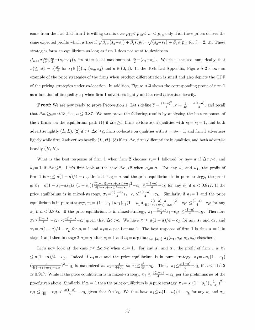
come from the fact that firm 1 is willing to mix over 11 12 1 only if all these prices deliver the

same expected profits which is true ifp+(2−1) + 21=

p(2−1) + 1111 for = 2. These

strategies form an equilibrium as long as firm 1 does not want to deviate to

+1221(22 −(2−1)) its other local maximum at 2

2 −(2−1). We then checked numerically that

∗1≤ (1− ) 24 for 1∈ [b( 1)2 2) and ∈ (0 1). In the Technical Appendix, Figure A-2 shows anexample of the price strategies of the firms when product differentiation is small and also depicts the CDF

of the pricing strategies under co-location. In addition, Figure A-3 shows the corresponding profit of firm 1

as a function of its quality 1 when firm 1 advertises lightly and its rival advertises heavily.

Proof: We are now ready to prove Proposition 1. Let’s define = (1−)24 , = 1

48 − (1−)4 , and recall

that ∆ ≥= 013, i.e., ≤ 087. We now prove the following results by analyzing the best responses ofthe 2 firms: on the equilibrium path (1) if ∆ ≥, firms co-locate on qualities with 1= 2= 1, and both

advertise lightly (); (2) if ≥ ∆ ≥, firms co-locate on qualities with 1= 2= 1, and firm 1 advertises

lightly while firm 2 advertises heavily (); (3) if ∆, firms differentiate in qualities, and both advertise

heavily ().

What is the best response of firm 1 when firm 2 chooses 2= 1 followed by 2= if ∆ and

2= 1 if ∆ ≤. Let’s first look at the case ∆ when 2= . For any 1 and 1, the profit of

firm 1 is 1≤ (1− )4− . Indeed if 1= and the price equilibrium is in pure strategy, the profit

is 1= (1− 1+1)1(1− 1)(2(1−)(1−1+1)+4(1−1+1)2−21 )

2− ≤(1−)4 − for any 1 if 0877. If the

price equilibrium is in mixed-strategy, 1=(1−)4 1−≤(1−)

4 −. Similarly, if 1= 1 and the priceequilibrium is in pure strategy, 1= (1− 1+1)1(1− 1)(

2(1−)+4(1−1+1)−1 )

2 − ≤ (1−)4 − for any

1 if 0895. If the price equilibrium is in mixed-strategy, 1=(1−)4 1− ≤ (1−)4 − . Therefore

1≤ (1−)4 − (1−)4 − given that ∆ . We have 1≤ (1− )4− for any 1 and 1, and

1= (1− )4− for 1= 1 and 1= per Lemma 1. The best response of firm 1 is thus 1= 1 in

stage 1 and then in stage 2 1= after 1= 1 and 1=argmax1∈{1} 1(1 2; 1 2) elsewhere.

Let’s now look at the case ≥ ∆ when 2= 1. For any 1 and 1, the profit of firm 1 is 1

≤ (1− )4− . Indeed if 1= and the price equilibrium is in pure strategy, 1= 1(1− 1)

( 4(1−1+1)−1 )

2− is maximized at 1=4

4+3 so 1≤2

48−. Thus, 1≤(1−)4 − if 1112

' 0917. While if the price equilibrium is in mixed-strategy, 1 ≤ (1−)4 − per the preliminaries of the

proof given above. Similarly, if 1= 1 then the price equilibrium is in pure strategy, 1= 1(1− 1)(1

4−1 )2−

≤ 148 − (1−)

4 − given that ∆ . We thus have 1≤ (1− )4− for any 1 and 1,

37

and 1= (1− )4− for 1= 1 and 1= per Lemma 1. The best response of firm 1 is thus to choose

1= 1 and 1= , and 1=argmax1∈{1} 1(1 2; 1 2) elsewhere. The last case to consider is∆ ≤when 2= 1. For any 1 and 1, the profit of firm 1 is 1≤ 148− . Indeed just like in the previous case,

if 1= , 1 ≤(1−)4 − if 1112 ' 0917. Given that ∆ ≤, 1≤ 148− . Then if 1= 1, the

price equilibrium is in pure strategy, 1= 1(1− 1)(1

4−1 )2−≤ 1

48− . We have 1≤ 148− for

any 1 and 1, and 1= 148− for 1= 47 and 1= 1. The best response of firm 1 is thus to choose

1= 47 in stage 1 and then in stage 2 1= 1 after 1= 47 and 1=argmax1∈{1} 1(1 2; 1 2)

elsewhere.

We now need to check firm 2’s best response to firm 1’s strategy. Let’s look at the same three cases. First,

when ∆ , firm 2 has a profitable deviation only if it can get a profit (1− )4− . Given that

1= 1, for any 2 and (1 2), the profit of firm 2 is 2≤ (1− )4− . Hence, no profitable deviation

exists for firm 2. Let’s now consider ≥ ∆ , firm 2 has a profitable deviation only if it can get a profit

(1− )4− . Given that 1= 1, for any 2 and (1 2), the profit of firm 2 is 2≤ (1− )4−

and 2≤ (1− )4− otherwise, so no profitable deviation exists for firm 2.

When∆ ≤ and 1= 47, if firm 2 chooses 2= 1 then () follows. A potential profitable deviation

is to locate close enough to 1= 47 to generate (). The first question is whether firm 2 makes

more profit in that case. If 2 ∈ [47 7(12(1− ))], the profit of firm 2 after () is not larger

than 748− . If 2 ∈ (7(12(1− )) 1], the profit of firm 2 after () is larger than 748− .

Note that 7(12(1− )) 1b( 1), so () leads to a mixed strategy equilibrium in price for 2 ∈(7(12(1− )) 1b( 1)). The next question is whether () will arise after a deviation of firm 1 at

the product stage. This will not be the case if the best response of firm 1 to 2= 1 is 1= 1. Let’s consider

that firm 2 chose 2 ∈ [7(12(1− ) 1] and firm 1 1= 47. The profit of firm 1 after () is lower

than (1− )(47)4− when 2 ∈ [7(12(1− )) 1b( 1)] per the preliminaries of the proof givenabove and is decreasing with respect to 2 when 2 ∈ [1b( 1) 1]. We also know that the profit of firm 1

after () is increasing with respect to 2 when 2 ∈ [1 1]. Therefore a sufficient condition for the bestresponse of firm 1 to 2= 1 is 1= 1 is that the profit when 1= 47, 2= 7(12(1− )) and () is

larger than (1− )4− . So when ∆ ≤21(2−1)(42−1)2 |1=47 2=7(12(1−))−(1− )(47)4 ≡, firm 2

does not have any profitable deviation from 1= 47 and 2= 1. We note for completeness that in a small

region of the product differentiation case (close to the interface with the advertising differentiation case),

1= 47, 2= 1 and () might not be an equilibrium because firm 2 might deviate to a lower quality

product in the first stage leading to (). In that case, the equilibrium might entail mixed strategies at

38

Figure 3: Average Price Levels (for firm 2 on the left and firm 1 on the right) in the Different Equilibria

the advertising stage and/or at the product location stage which falls beyond the scope of this paper.

Figure 3 depicts the average prices in the various sub-game pricing equilibria as a function of the adver-

tising impact differential (∆), conditional on each firm selecting the corresponding quality and advertising

levels of the No Differentiation, Advertising Differentiation and Product Differentiation cases.

Proof of Corollary 1

The proof of Proposition 1 covers the subcase ∆ = 0. Specifically, when ∆ = 0 ⇔ ∆ 12+

1√6

' 091 then advertising differentiation occurs in equilibrium. When ∆ = 0 ⇔ ∆ 12+

1√6then

product differentiation occurs in equilibrium.

Proof of Proposition 2

The comparative statics of 1 and 2 wrt ∆ are derived from the expressions of the profits in the three

types of equilibria.

Proof of Proposition 3

Formally, the targeting strategy of firm , denoted by , can be ∅, L, H, or ∪ . The costs associated withthe four possible advertising strategies are 0 , respectively. First, we examine the pricing stage

of the game given the quality levels and the advertising segments in 9 possible different cases. 1- the two

segments are distinct, that is, if 1∩2 = ∅. 2- both firms choose both intervals, that is , if 1 = 2 = ∪.

39

3- the firms choose the same intervals 1 = 2 = . 4- the firms choose the same interval 1 = 2 = . 5-

1 = and 2 = ∪. 6- 1 = ∪ and 2 = . 7- 1 = and 2 = ∪. 8- 1 = ∪ and 2 = .

9- each firm is a monopolist in its segment or one firm does not advertise and the other is a monopolist. The

details of the price equilibrium in each of these cases is provided in the Technical Appendix.

We now turn our attention to the advertising stage of the game and determine which segments firms

choose to advertise to. Let us examine the different types of possible equilibria. An equilibrium is described

by a pair (1 2), where the first set denotes the segment(s) chosen by firm 1 and the second set denotes

the segment(s) chosen by firm 2. First we fix 1 2 and determine which types of equilibria are possible

if 23 ≥ ≥ 13. Note that we do not consider cases where a firm does not advertise. We analyze the

following cases in the Technical Appendix: (), (∪), (∪), (), and (∅ ) or ( ∅). In thefollowing cases, we show in the Technical Appendix that one of the firms always has an incentive to deviate,

thus, they do not constitute equilibria. We assume that firms make positive profits, otherwise it would be

profitable for them to not advertise at all: ( ∪ ∪), (), (), ( ∪), and ( ∪).

If now we fix 1 = 2, then in the cases where |1 ∩ 2| 0, we show that firms always have an

incentive to deviate. When the target segments are exactly the same, prices are zero, hence firms have a

straightforward incentive to deviate. There are two other cases with an intersection and non-zero profits: (1)

when one firm advertises to both segments and the other to only the low segment (say ( ∪), w.l.o.g).In this case, firm 2’s profits before advertising are exactly the same as in the case of (), hence firm 2

will deviate to this to save on advertising costs (because 0). (2) when non-identical targets are chosen

(say ( ∪), w.l.o.g), firm 1’s profits before advertising are exactly the same as in the case of (),

hence firm 1 will deviate to the latter to save on advertising costs. Therefore, in the case of 1 = 2, the

only possible advertising equilibria are = and = . In this case, firms do not have an incentive to

deviate as long as 23 ≥ ≥ 13.

Fixing 1 2, we have different patterns of equilibria depending on the parameter values. In all

cases, low enough quality levels will make the costs of advertising prohibitively high for at least one firm

resulting in a (partial) no advertising equilibrium. If costs are sufficiently low, the following equilibrium

pattern emerges: Starting with 12 ≤ 23, the unique advertising equilibrium is ( ∪) when 12

is small as defined by (??). When 12 is larger than that threshold, () is an equilibrium. This is a

unique equilibrium when 12 is in a medium range such that 12 is below the threshold defined by (??).

Above this threshold, the () equilibrium is not unique and () is an additional equilibrium. When

40

13 12, the equilibrium structure is similar, but for low values of 12 (as defined by (??)) the

unique equilibrium is (∪). For medium and high values of 12, we have a unique () equilibrium

and multiple () and () equilibria as before.

Now we can examine the first (quality choice) stage of the game. We first show that a quality choice pair

whereby both qualities are set at 1 cannot be an equilibrium. Note that firm 2’s revenue is increasing in 2

in all advertising subgames, therefore firm 2 always has an incentive to increase its quality to the maximum

given the advertising equilibrium. Also, increasing quality never causes the advertising equilibrium to change

in a way that hurts firm 2. Therefore, in equilibrium 2 = 1 must hold. Firm 1’s situation differs depending

on . First, when firm 1 does not advertise, it always has the incentive to increase its quality and advertise.23

Next, we analyze the cases where both firms advertise, starting with 23 ≥ 12. When 1 is small

the advertising equilibrium is ( ∪). In this case firm 1 has an incentive to increase its quality up to

47. However, this advertising equilibrium only possibly holds for ̄(12) and the highest possible 1

value is reached in this region as ̄(1)= 23 at 1 = 3√3 − 5 47; therefore firm 1 wants to increase

its quality. In the other advertising equilibria, () and (), firm 1 acts as a monopolist and trivially

wants to increase its quality as long as that player does not expect the advertising equilibrium to change.

One potential Nash-equilibrium exists when 1 = ∗1 1 with the () advertising strategies. This is a

subgame perfect Nash-equilibrium if player 2 commits to setting 2 = for all 1 ∗1. However, this

equilibrium is Pareto dominated by the one where 1 = 2 = 1 and 1 = and 2 = .

When 12 13, the analysis is similar. For low values of 1, the advertising equilibrium is

( ∪ ). However, in this case firm 1 may reach 1 = 47 to maintain this type of equilibrium. One

can then check that the profit firm 1 makes in this equilibrium 148− is strictly less than when setting

1 = 1 and attaining the () equilibrium with profits of 24 − as long as 13. Therefore, the

only equilibria are the ones without overlapping advertising segments and then the same logic applies as in

the previous case. Finally, when 1 = 2, it is clear that neither firm has an incentive to decrease its quality

given the above comparisons, completing the proof of the proposition.

Proof of Corollary 2

When ≤ 12, per Proposition 3, 1 = 2 = 1, 1 = and 2 = with firm 2 choosing the monopolist

price for its target segment 2=12 . A consumer in 2 either buys the product of firm 2 or does not buy

since that consumer is not aware of the existence of the rival’s product. Such a consumer buys if and only

23Since we assume 148 there is always a way for firm 1 to make positive profits by advertising.

41

if 2−2≥ 0 or ≥12 . Recall that 2 corresponds to ∈ [ 1]. Therefore there exists a pocket ∈ (12)of unserved consumers.

Proof of Corollary 3

Per Proposition 3, 1 = 2 = 1, 1 = , 2 = , 1=2 and 2= max(

12 ). Thus 1=

2 and 2=

12 when

∈ [13 12 ] and 2 = 1− when ∈ [12 23 ]. Finally 1+2=1+2 when ∈ [13 12 ] and 1−

2 when ∈ [12 23 ].The comparative statics for the demands follow from these expressions.

References

Ackerberg, D., A. (2001). Empirically distinguishing informative and prestige effects of advertising. RAND

Journal of Economics 32, 316—333.

Archibald, R., B., C. H. Haulman, and C. E. M. Jr. (1983). Quality, price, advertising, and published quality

ratings. Journal of Consumer Research 9, 347—356.

Bagwell, K. (2007). Chapter 28 the economic analysis of advertising. 3, 1701—1844.

Banker, R. D., I. Khosla, and K. K. Sinha (1998). Quality and competition. Management Science 44 (9),

1179—1192.

Bester, H. (1998). Quality uncertainty mitigates product differentiation. The RAND Journal of Economics,

828—844.

Butters, G. (1977). Equilibrium distributions of sales and advertising prices. Review of Economic Studies 44,

465—491.

Caves, R., E. and D. P. Greene (1996). Brands’ quality levels, prices, and advertising outlays: Empirical

evidence on signals and information costs. International Journal of Industrial Organization 14, 29—52.

Chen, Y., C. Narasimhan, and Z. J. Zhang (2001). Individual marketing with imperfect targetability.

Marketing Science 20 (1), 23—41.

Choi, C. J. and H. S. Shin (1992). A comment on a model of vertical product differentiation. The Journal

of Industrial Economics 40 (2), 229—231.

Choudhary, V., A. Ghose, T. Mukhopadhyay, and U. Rajan (2005, July). Personalized pricing and quality

differentiation. Management Science 51 (7), 1120—1130.

Eechambadi, N. T. (1994). Does advertising work? The McKinsey Quarterly 3, 117—130.

Erdem, T., M. P. Keane, and B. Sun (2008). A dynamic model of brand choice when price and advertising

signal product quality. Marketing Science 27 (6), 1111—1125.

42

Gabszewicz, J. J. and J.-F. Thisse (1979). Price competition, quality and income disparities. Journal of

economic theory 20 (3), 340—359.

Gotter, A. (2018, May). The complete resource to understanding facebook ads cost - 2017 benchmarks.

AdEspresso by Hootsuite. https://adespresso.com/blog/facebook-ads-cost/.

Grossman, G. M. and C. Shapiro (1984). Informative advertising with differentiated products. The Review

of Economic Studies 51 (1), 63—81.

Hauser, J. R. and B. Wernerfelt (1990). An evaluation cost model of consideration sets. Journal of Consumer

Research 16 (4), 393—408.

Iyer, G., D. Soberman, and J. M. Villas-Boas (2005). The targeting of advertising. Marketing Science 24 (3),

461—476.

Jing, B. (2006, May-June). On the profitability of firms in a differentiated industry. Marketing Science 25 (3),

248—259.

Kane, L. (2014). Here’s when you should buy store brand food. Business Insider . September, 12.

Kash, B. A. and T. R. Miller (2009). The relationship between advertising, price, and nursing home quality.

Health Care Management Review 34 (3), 242—250.

Keller, K. L. and P. Kotler (2011). Marketing Management (14 ed.). Upper Saddle River, New Jersey:

Pearson Prentice Hall.

Knudsen, T. R. (2006). Escaping the middle-market trap: An interview with the CEO of Electrolux. The

McKinsey Quarterly (4), 72—79.

Knudsen, T. R., A. Randel, and J. Rugholm (2005). The vanishing middle market. The McKinsey Quar-

terly (4), 6—9.

Lauga, D. O. and E. Ofek (2009). Market research and innovation strategy in a duopoly. Marketing

Science 28 (2), 373—396.

Levin, R. C., A. K. Klevorick, R. R. Nelson, S. G. Winter, R. Gilbert, and Z. Griliches (1987). Appropriating

the returns from industrial research and development. Brookings Papers on Economic Activity; Special

Issue on Microeconomics (3), 783—831.

Mayzlin, D. and J. Shin (2011). Uninformative advertising as an invitation to search. Marketing Sci-

ence 30 (4), 666—685.

McAfee, R., P. (1994). Endogenous availability, cartels, and merger in an equilibrium price dispersion.

Journal of Economic Theory 62, 24—47.

Milgrom, P. and J. Roberts (1986). Price and advertising signals of product quality. Journal of Political

Economy 94, 796—821.

43

Mitra, A. and J. G. Lynch (1995). Toward a reconciliation of market power and information theories of

advertising effects on price elasticity. Journal of Consumer Research (3), 644—659.

Mohammed, R. (2011, January-February). Ditch the Discounts. Harvard Business Review .

Moorthy, K. S. (1988, Spring). Product and price competition in a duopoly. Marketing Science 7 (2), 141—168.

Narasimhan, C. (1988). Competitive promotional strategies. Journal of Business 61 (4), 427—449.

Nelson, P. (1974). Advertising as Information. Journal of Political Economy 82, 729—754.

Ofek, E. and M. Hamid (2005). Brocade: Launching the multiprotocol router. HBS Case No. 505064 . HBS

Publishing.

Rhee, B.-D. (1996, Feb). Consumer heterogeneity and strategic quality decisions. Management Science 42 (2),

157—172.

Ries, A. (2011). Hi-Lo: How you can target both ends of the market. AdAge. December, 7.

Roy, S. (2000). Strategic Segmentation of a Market. International Journal of Industrial Organization 18,

1279—1290.

Shaked, A. and J. Sutton (1982). Relaxing price competition through product differentiation. Review of

Economic Studies XLIX, 3—13.

Soberman, D. (2005). The complexity of media planning today. Journal of Brand Management 12 (6),

420—429.

Song, R., S. Jang, and G. Cai (2016). Does advertising indicate product quality? Evidence from prelaunch

and postlaunch advertising in the movie industry. Marketing Letters 27 (4), 791—804.

Stuart, A. (2011). Apple’s message: No discounts. CFO Magazine. November, 1.

Tellis, G., J. and C. Fornell (1988). The relationship between advertising and product quality over the

product life cycle: A contingency theory. Journal of Marketing Research 25, 64—71.

Thomas, O. C., C. T. Allen, and R. J. Semenik (2000). Advertising2. South-Western, Thomson Learning.

Tirole, J. (1988). The Theory of Industrial Organization. Cambridge, MA: MIT Press. Ch. 7.

Varian, H. (1980). A model of sales. The American Economic Review 70 (4), 651—659.

Wauthy, X. (1996, Sep). Quality choice in models of vertical differentiation. Journal of Industrial Eco-

nomics 44 (3), 345—353.

Zhang, K. and Z. Katona (2012). Contextual Advertising. Marketing Science 31 (6), 980—994.

Zhu, Y. and A. Dukes (2017). Prominent Attributes Under Limited Attention. Marketing Science 36 (5),

683—698.

44