what’s new in microsoft excel 2007? -...
TRANSCRIPT

What’s New in Microsoft Excel 2007? Olathe District Schools Instructional Technology
Last Updated ~ July, 2008

New
Fe
atu
res
in
Mic
roso
ft E
xcel
200
7 -
Ola
the
Dis
tric
t S
cho
ols
1
Introduction to MS Excel 2007
This tutorial is for you if you've used a previous version of Excel. Here you'll find an overview of what's
new and what's changed in Excel 2007. You have already been introduced to the overall new features in
Microsoft Office 2007, such as the Microsoft Office Button, Tabs and Ribbons, and Groups and
Commands. The New User Interface makes every feature easy to locate and use. Those features will
not be re-introduced in this training. However, there are unique Tabs, Groups and Commands you will
want to familiarize yourself with in Excel 2007, as well as significant changes in the way certain functions
and formulas are handled by Excel 2007.
Open Microsoft Excel 2007.
Save the new workbook as: Excel 2007 Practice.
The New Look of Excel 2007

New
Fe
atu
res
in
Mic
roso
ft E
xcel
200
7 -
Ola
the
Dis
tric
t S
cho
ols
2
New Modern-Looking Fonts
The default workbook font is now 11-point Calibri, which is much more readable than the old 10-point
Arial, especially in smaller sizes. There are also additional fonts available in this new version.
New File Formats
Excel’s xls file format has become a recognized industry standard. Excel 2007 still supports that format,
but it now uses new default “open” file formats that are based on XML (Extensible Markup Language).
For compatibility, Excel 2007 still supports the old file formats so that you can continue to share your
work with those who haven’t upgraded to Excel 2007. The new file format provides for smaller file sizes,
less chance of file corruption and other security attributes.
File Compatibility
For backward compatibility and collaboration with earlier versions of Microsoft Office Excel, you can use
one of two ways to open Microsoft Office Excel 2007 workbooks in an earlier version of Excel. You can
either use the earlier file format (.xls) or the new XML-based file format (.xlsx) to exchange workbooks
between different versions of Excel. Office Excel 2007-specific features and formatting may not be
displayed in the earlier version of Excel, but they are still available when the workbook is saved and
then re-opened in Excel 2007.
To ensure that a workbook that you save in Office Excel 2007 can be opened in an earlier version of
Excel, you can save a copy that is fully compatible with Excel 97-2003 (.xls) in Excel 2007.
Users who use an earlier version of Excel can also download the Microsoft Office Compatibility Pack for
2007 Office Word, Excel and PowerPoint File Formats to install updates and converters for the earlier
version of Excel. This allows them to open, edit, and save an Excel 2007 workbook in the earlier version
of Excel, without having to save it to that version's file format first.

New
Fe
atu
res
in
Mic
roso
ft E
xcel
200
7 -
Ola
the
Dis
tric
t S
cho
ols
3
New Worksheet Functions
There are several new functions available in Excel 2007. They include:
AVERAGEIF and AVERAGEIFS
Calculates a conditional average (similar to SUMIF and COUNTIF examples shown below).
SUMIFS
Calculates a conditional sum using multiple criteria.
Weight 18
29
36
11
16
Using the
SUMIF function
65
COUNTIFS
Calculates a conditional COUNT using multiple criteria.
Salesperson Invoice
Buchanan 15,000
Buchanan 9,000
Suyama 8,000
Suyama 20,000
Buchanan 5,000
Dodsworth 22,500
Formula Description (Result)
=COUNTIF(B2:B7,">9000") Numbers above 9000 (3)
=COUNTIF(B2:B7,"<=9000") Numbers less than or equal to 9000 (3)
PRACTICE:
You can add numbers based on a single criterion by using the SUMIF function or
by using a combination of the SUM and the IF functions.
For example, the formula =SUMIF(A2:A6,">20") adds only the numbers in the
range A2 through A6 that are greater than 20.
PRACTICE:
Let's say you want to count how many
salespeople exceeded their sales goals for a
quarter or how many stores under-performed
compared to an industry average for yearly
revenues. To count numbers greater than or
less than a number, use the COUNTIF
function.
For example, the formula
=COUNTIF(B2:B7,">9000") counts only the
numbers in the range B2 through B7 that are
greater than 9000.

New
Fe
atu
res
in
Mic
roso
ft E
xcel
200
7 -
Ola
the
Dis
tric
t S
cho
ols
4
IFERROR
Returns a value you specify if a formula evaluates to an error; otherwise, returns the result of the
formula. See example below. If the division is not possible, the phrase entered is displayed.
More Functions
In addition, 39 worksheet functions that used to require the Analysis Toolpak add-in are now built-in.
Excel 2007 also includes seven new CUBE functions that retrieve data from SQL Server Analysis Services.
These are advanced functions and ones that the “average” Excel 2007 user will most likely never use.
Worksheet Tables
Working with tables is easier than ever. When you create a table (previously known as a list) in a
Microsoft Office Excel worksheet, you can manage and analyze the data in that table independently of
data outside the table. For example, you can filter table columns, add a row for totals, and apply table
formatting to the table. A table is just a rectangular range of cells that usually contains column headers.
Once you designate a particular range to be a table using either the Home > Styles > Format as Table
Command or the the Insert > Tables > Table command, Excel provides you with some very efficient
tools that work with the table:
You can apply attractive formatting with a single click.
You can easily insert summary formulas in the table’s total row.
If each cell in a column contains the same formula, you can edit one of the formulas, and the
others change automatically.
You can easily toggle the display of the table’s header row and totals row.
Auto-filtering and sorting options have been expanded.
If you create a chart from a table, the chart will always reflect the data in the table—even if you
add new rows.
If you scroll a table downwards so that the header row is no longer visible, the column headers
now display where the worksheet column letters would be.

New
Fe
atu
res
in
Mic
roso
ft E
xcel
200
7 -
Ola
the
Dis
tric
t S
cho
ols
5
Create a Table
Create a new table in Excel by entering the following data in a new worksheet.
Format the cells similar to what is shown above, using the Home Tab, Styles Group, Cell Styles
Command.
Highlight the range A2:E6. Do not highlight cell A1.
Click the Format as Table command in the Styles Group.
Choose the Table Style Medium 25 from the Styles Window.
Since our table has headings in Row 2, verify that this checkbox is selected. Click OK.
Olathe High School Enrollment 2007-2008
QTR1 QTR2 QTR3 QTR4
OE 1512 1510 1522 1502
ON 1310 1315 1317 1315
ONW 1385 1388 1387 1390
OS 1489 1479 1485 1490
New
Fe
atu
res
in
Mic
roso
ft E
xcel
200
7 -
Ola
the
Dis
tric
t S
cho
ols
6
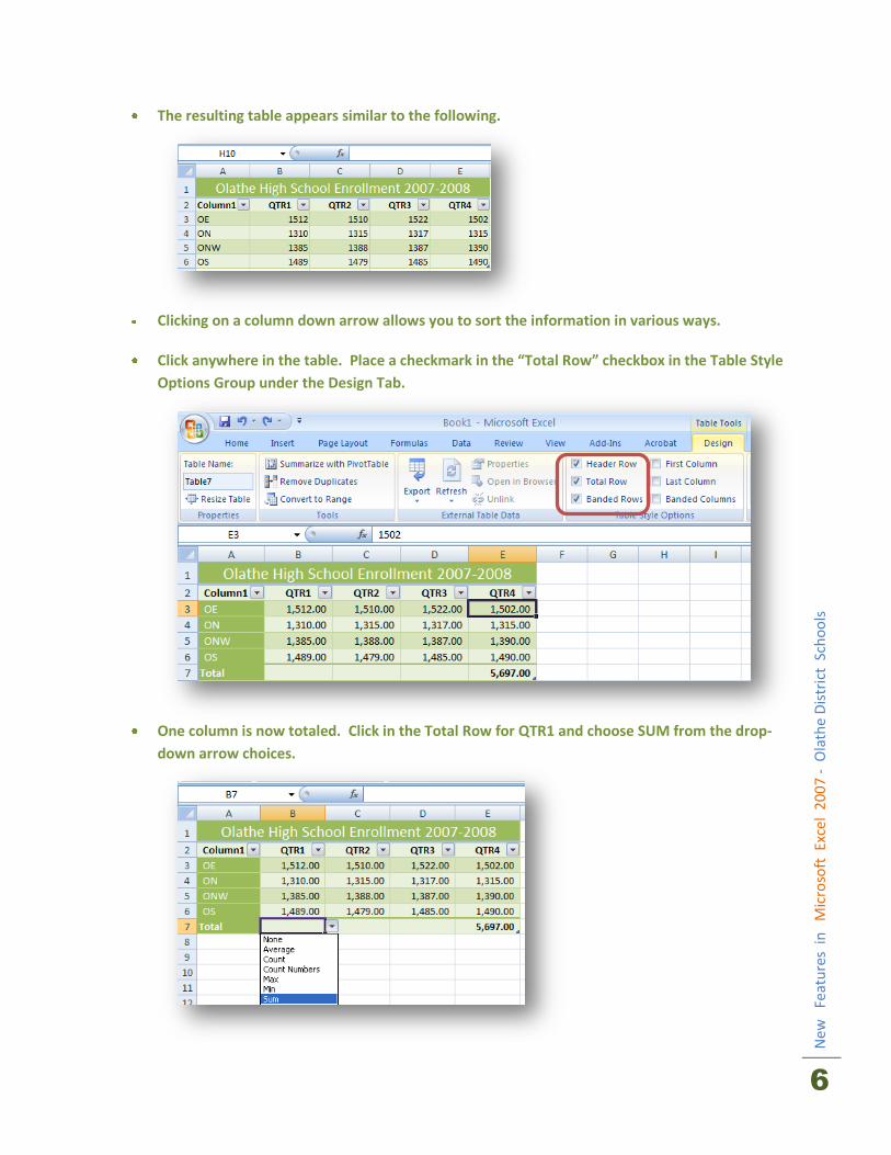
The resulting table appears similar to the following.
Clicking on a column down arrow allows you to sort the information in various ways.
Click anywhere in the table. Place a checkmark in the “Total Row” checkbox in the Table Style
Options Group under the Design Tab.
One column is now totaled. Click in the Total Row for QTR1 and choose SUM from the drop-
down arrow choices.

New
Fe
atu
res
in
Mic
roso
ft E
xcel
200
7 -
Ola
the
Dis
tric
t S
cho
ols
7
Let your mouse rest on the bottom right corner of cell B7. The cursor turns into a single
crosshair, drag to the right 2 cells to fill this formula into cell C7 and cell D7.
Insert a column to the right of QTR4 by clicking in the QTR4 column in row 3 and choosing the
Insert Table Column to the Right command from the Table Tools Design Tab.
Enter the column heading “Average” in this new column.
Click the Formulas Tab and from the AutoSum command, choose “Average”.
Press ENTER.
Notice the Average function fills down to the remaining 3 school rows.

New
Fe
atu
res
in
Mic
roso
ft E
xcel
200
7 -
Ola
the
Dis
tric
t S
cho
ols
8
Change the decimal placement formatting, if needed, using the Decrease Decimal command
from the Home Tab, Number Group.
Converting the Table Back to a Data Range
To Convert this Table back to a Data Range, click anywhere in the table.
Click the Table Tools Design Tab. Choose Convert to Range in the Tools Group.

New
Fe
atu
res
in
Mic
roso
ft E
xcel
200
7 -
Ola
the
Dis
tric
t S
cho
ols
9
Click “Yes” at the resulting dialog box.
The result is a normal range of populated cells. The sorting arrows are no longer available.
You may delete the “Column 1” text in cell A2 if desired.
Format the table further using the Cell Styles command as this feature is still available.
Olathe High School Enrollment 2007-2008 QTR1 QTR2 QTR3 QTR4
OE 1512 1510 1522 1502
ON 1310 1315 1317 1315
ONW 1385 1388 1387 1390
OS 1489 1479 1485 1490
Olathe High School Enrollment 2007-2008 QTR1 QTR2 QTR3 QTR4
OE 1,512.00
1,510.00
1,522.00
1,502.00
ON 1,310.00
1,315.00
1,317.00
1,315.00
ONW
1,385.00
1,388.00
1,387.00
1,390.00
OS
1,489.00
1,479.00
1,485.00
1,490.00

New
Fe
atu
res
in
Mic
roso
ft E
xcel
200
7 -
Ola
the
Dis
tric
t S
cho
ols
1
0
Larger Worksheets
A worksheet now has 1,048,576 rows and 16,384 columns, which computes to more than 17 billion cells.
An Excel 2007 worksheet has more than 1,000 times as many cells as an Excel 2003 worksheet.
Excel 2003 versus Excel 2007
Excel 2003 Excel 2007
Number of rows 65,536 1,048,576
Number of columns 256 16,384
Amount of memory used 1 Gbyte Maximum allowed by Windows
Number of colors 56 4.3 billion
Number of conditional formats per cell 3 Unlimited
Number of levels of sorting 3 64
Number of levels of undo 16 100
Number of items shown in the Auto-Filter dropdown 1,000 10,000
The total number of characters that can display in a cell 1,000 32,000
Number of unique styles in a workbook 4,000 64,000
Maximum number of characters in a formula 1,000 8,000
Number of levels of nesting in a formula 7 64
Maximum number of function arguments 30 255
Maximum number of function arguments 30 255

New
Fe
atu
res
in
Mic
roso
ft E
xcel
200
7 -
Ola
the
Dis
tric
t S
cho
ols
1
1
Styles and Themes
Excel has always supported named styles, which can be applied to cells and ranges. Excel 2007 brings
this feature to the forefront by providing a good assortment of predefined styles, easily accessible by
choosing Home > Styles > Cell Styles.
With the introduction of document themes, Excel 2007 makes it easy to create good-looking
worksheets. A theme consists of a color palette, font set, and effects. You now have one-click access to
a gallery of professionally-designed themes that can dramatically change the look of your entire
spreadsheet—almost always for the better. Access the theme gallery by choosing
Page Layout > Themes > Themes.

New
Fe
atu
res
in
Mic
roso
ft E
xcel
200
7 -
Ola
the
Dis
tric
t S
cho
ols
1
2
Better Looking Charts
Excel 2007 offers no new chart types. However, Excel charts now look better than ever. For the first
time, Microsoft uses the term “boardroom quality” to describe the new look to Excel 2007 charts.
Create a Chart
Highlight cells A2:E6 to select them.
Click on the Insert Tab and choose Column.
Choose the 1st Cylinder icon.

New
Fe
atu
res
in
Mic
roso
ft E
xcel
200
7 -
Ola
the
Dis
tric
t S
cho
ols
1
3
By Default, Charts are automatically inserted in the same spreadsheet as their respective data
in Excel 2007. Drag the chart and resize it as shown below.
Click inside the data area of the table.
Change the Theme. Notice the chart theme also updates.

New
Fe
atu
res
in
Mic
roso
ft E
xcel
200
7 -
Ola
the
Dis
tric
t S
cho
ols
1
4
Chart Tools Contextual Tab Use the Chart Tools Design Tab to change the Chart Style to a style similar to that shown
below.
Use the Chart Tools Layout Tab to add a Chart Title and Axis Titles as shown above.
If you would prefer the chart be located on a different worksheet, right-click on the chart and
choose “Move Chart”. Choose “New Sheet”.

New
Fe
atu
res
in
Mic
roso
ft E
xcel
200
7 -
Ola
the
Dis
tric
t S
cho
ols
1
5
Page Layout View
As an option, you can display your worksheet as a series of pages. This new Page Layout view ensures no
surprises when it’s time to print your work. Even better, the Page Layout view includes “click and type”
page headers and footers—which is much more intuitive than the old method. Unlike the standard print
preview, Page Layout view is fully functional in terms of spreadsheet editing.
Excel’s new Page Layout view makes it easy to see how your printed work will appear.
Enhanced Conditional Formatting
Conditional formatting refers to the ability to format a cell based on its value. Conditional formatting
makes it easy to highlight certain values so that they stand out visually. For example, you may set up
conditional formatting so that if a formula returns a negative value, the cell background displays green.
In the past, a cell could have at most three conditions applied. With Excel 2007, you can format a cell
based on an unlimited number of conditions. But that’s the least of the improvements. Excel 2007
provides a number of new data visualizations: data bars, color scales, and icon sets.
Excel 2007 includes quite a few other improvements to conditional formatting. In general, conditional
formatting is much more flexible, easier to set up, and relies less on creating custom formulas to define
the formatting rules.

New
Fe
atu
res
in
Mic
roso
ft E
xcel
200
7 -
Ola
the
Dis
tric
t S
cho
ols
1
6
Practice Conditional Formatting
Highlight cells F3:F6
Click the “Conditional Formatting” option in the Styles Group under the Home Tab.
Choose New Rule from the drop-down menu.
Enter the New Formatting Rule as shown below. This rule will show a red “Alert” icon when
the enrollment average is >= 1400, a yellow “Warning” icon when the average is <1400 and
>=1300, and a green “OK” icon when the enrollment is <1300.
Time to
build a new
high school!

New
Fe
atu
res
in
Mic
roso
ft E
xcel
200
7 -
Ola
the
Dis
tric
t S
cho
ols
1
7
Formula AutoComplete
Entering formulas in Excel 2007 can be a bit less cumbersome, thanks to the new Formula
AutoComplete feature. When you begin typing a formula, Excel displays a continually updated drop-
down list of matching items, including a description of each item. When you see the item you want,
press Tab to enter it into your formula. The items in this list consist of functions, defined names, and
table references.
Structured Referencing
Excel 2007 applies structured referencing within formulas when you create a table. Structured
referencing automatically names table columns based on their headings (values in the top row), then
uses those names in formulas whenever possible. Formulas with structured referencing are easier to
read and less prone to errors because each cell can contain the exact same formula. It is more difficult
to change one accidentally. See example below.
Improved Pivot Tables
Excel’s pivot table feature is probably one of its most underutilized features. A pivot table can turn a
large range of raw data into a useful interactive summary table with only a few mouse clicks. Microsoft
has made this feature more accessible by improving just about every aspect of pivot tables in Excel
2007. Charts created from pivot tables (pivot charts) now retain their formatting when they’re updated.
This loss of formatting had been a frustration for many users in the previous version. This is a more
advanced feature and will not be covered in this introductory training.

New
Fe
atu
res
in
Mic
roso
ft E
xcel
200
7 -
Ola
the
Dis
tric
t S
cho
ols
1
8
Other New Features
PDF add-in:
You can create an industry-standard Adobe PDF file directly from Excel using an add-in available
from Microsoft.
More control over the status bar:
You can now control the type of information that appears in the status bar.
Color Schemes:
Change the appearance of Excel by applying one of three color schemes that ship with Excel
(Blue, Silver, or Black).
Resizable formula bar:
When editing lengthy formulas, you can increase the height of the formula bar so that it doesn’t
obscure your worksheet. Just click and drag on the bottom border of the formula bar.
Lots of new templates:
Why reinvent the wheel? Choose Office > New, and you can choose from a variety of templates.
One of them may be exactly (or at least close to) what you need.

New
Fe
atu
res
in
Mic
roso
ft E
xcel
200
7 -
Ola
the
Dis
tric
t S
cho
ols
1
9
The Lower Right Corner
Another efficient feature of 2007 Office is in the lower right corner of Word, Excel, PowerPoint
and Access. When you open these applications you will see that the “zoom” feature is now
available, as well as other logical “view” features for each application. The Excel View
commands for Normal, Page Layout and Page Break Views are located in the bottom right
corner of the Excel 2007 window, along with the Zoom Controls.
Microsoft Office Help Button
The Microsoft Office Help Button is located in the top right corner of all Office applications. You may also press the F1 function key on your keyboard to access Help.