What to do about salinitywhen a Assimilating XBT data?

Results for estimating salinity in theGulf of Mexico

and in theNorthwestern Atlantic Ocean

I’m Carlisle Thacker

and I approve of this message.

What to do when temperature is observed,but density is important?

• When XBT data are assimilated, salinity must be corrected along with temperature.

• Incorrect salinity causes incorrect density and currents.

• How to correct salinity without observing salinity?

Two regions as examples.

• Gulf of Mexico– Loop current, eddies.– Broad shelves with deep central basin.– River inflow.– Many bad data.

• Large North Atlantic region containing the Gulf Stream– Very large T and S variability.– Shelf in north but mostly deep ocean.– Gulf Stream inflow.– Few bad data.

Gulf of Mexico

3485 CTD stations –many redundant.

Most stations inshallow water.

Few in south.

No problem.

Sub-sampled to avoid near duplicates.

- 739 stations used.

Problems with archived data:

• Sampling is not uniform.– Local high-density sampling.– Few samples in south.

• Some data are bad.– Flags are not very helpful.

• Distributions are not Gaussian.– How to distinguish bad data from heavy tails?– Box and whisker plots are helpful.– TS plots also show outliers.

Distributions of T and S data in 20 dbar intervals.

A first look at the 3489 CTD profiles for Gulf of Mexico.

Warm outliers between 180 dbar and 200 dbarMostly good loop-current data.

All data between 180 dbar and 200 dbar

Notice bad data!

Some profiles have density inversions 37 with inversion greater than 0.01 kg/m3

Equal number of long verification and training profiles

More short verification profiles

TS plotstraining + verification data

• Data interpolated at 25 dbar pressure intervals.

• Mean T vs. mean S at all levels indicated in red on each panel.

• Warm-salty Loop Current values are not on mean TS curve.

Skill explaining independent data Estimated and observed salinityrobust parabola

pres

sure

(dba

r)

rms prediction error (psu)

0.01 psu at 900 dbar

0.20 psu at 50 dbar0.20 psu at 50 dbar

0.05 psu at 200 dbar

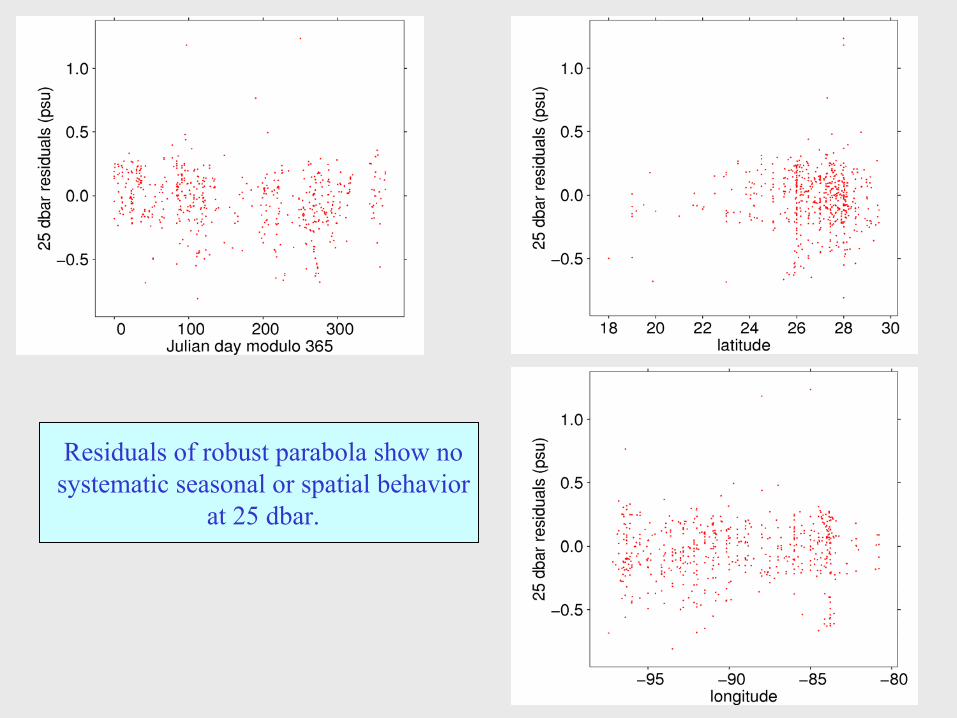
Residuals of robust parabola show no systematic seasonal or spatial behavior

at 25 dbar.

Stommel’s methodmisses Loop Current

200 dbar

0.05 psu

0.15 psu0.28 psu0.10 psu

Models derived from CTD data are considerably more accuratethan those inferred from climatology.

How good is density ?

Might want better near the surface.

Get same accuracy with regression models for density.

0.02 kg/m3

Northwest Atlantic

Gulf Stream station map

CTD stations in Northwestern Atlantic study area

Discarded data from shelf.

Bwplots for Gulf Stream Region

Distributions of CTD observations in NW Atlantic

TS plots at 4 levels

NW sub regionSE sub region

1390 stations with long profiles in northwestern Atlantic

Training and verification stations

NW sub-region

Skill explaining independent data

200 dbar

0.07 psu

0.02 psu

0.62 psu

0.75 psu 0.92 psu

NW sub-region

P4(T) residualsat 25 dbar

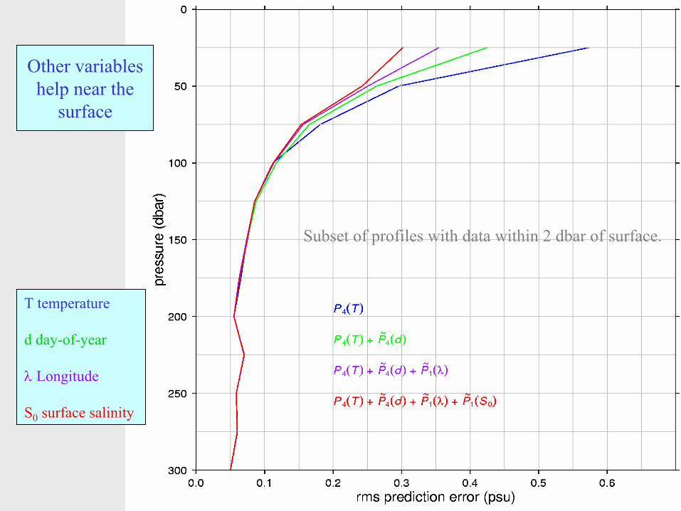
Other variables help near the

surface

Subset of profiles with data within 2 dbar of surface.

T temperature

d day-of-year

λ Longitude

S0 surface salinity

Estimatedvs.

observed

28randomlyselected

NWprofiles

Calibration error?

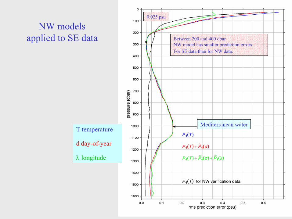
NW modelsapplied to SE data

T temperature

d day-of-year

λ longitude

Between 200 and 400 dbarNW model has smaller prediction errorsFor SE data than for NW data.

0.025 psu

Mediterranean water

SE sub-region

Skill explainingindependent SE data

T temperatureλ longitudeφ latituded day-of-year

0.02 psu

SE models

0.02 psu

0.04 psu with latitude as a predictor

NW profiles

NW modelSE model

SE profiles

Performance near partition

Regression beatsNavy’s MODAS systemin Gulf Stream triangle.

Best regression modelfor NW sub-region

(Gulf Stream and its eddies)P4(T)+P4(d)+P1( )

4th degree in temperature4thin day of year1st in longitude

MODAS

Except near the surfaceregression beats

Navy’s MODAS systemin Sargasso Sea triangle.

Best regression modelfor SE sub-region

(Sargasso Sea)P2(T)+P1(ϕ)+P1( )

2nd degree in temperature1st in latitude and longitude

MODAS

0.1 psu

Regression beatsNavy’s MODAS system

in Gulf of Mexico.

Best regression modelfor Gulf of Mexico

P4(T)4th degree in temperature

MODAS

0.25 psu 1.25 psu

Conclusions:

• Regression beats using climatological T and S.• Can handle fronts.• Where to draw regional boundaries?• Accurate near-surface estimates are difficult.• Can use to check salinity calibration in CTD archives.• Can also check ARGO float calibration.• Big ocean – still lots of work to do.• Can use MODAS until more regions are modeled.• MODAS is being reworked.