what is the expected return on a stock? - centre for finance · what is the expected return on a...

What is the Expected Return on a Stock?

Ian Martin Christian Wagner∗

May 2016

Abstract

We derive a formula that expresses the expected return on a stock in terms

of the risk-neutral variance of the market, the stock’s idiosyncratic risk-neutral

variance, and average idiosyncratic risk-neutral variance. These components can

be computed from the prices of index and stock options. We test the formula

by running predictive panel regressions at the individual stock level. We conduct

joint hypothesis tests and find, in most of our specifications, that the estimated

coefficients are significantly different from zero and insignificantly different from

the values predicted by our theory. When coefficients are fixed at the levels

implied by our theory, the formula—which has no free parameters—outperforms

a range of competitors in predicting individual stock returns.

∗Martin: London School of Economics. Wagner: Copenhagen Business School. We thank JohnCampbell, Christian Julliard, Dong Lou, Marcin Kacperczyk, Stefan Nagel, Tarun Ramadorai, AndreaTamoni, Paul Schneider and Dimitri Vayanos for their comments. Ian Martin thanks the ERC fortheir support under Starting Grant 639744. Christian Wagner acknowledges support from the Centerfor Financial Frictions (FRIC), grant no. DNRF102.

1

In this paper, we derive a new formula that expresses the expected return on an

individual stock in terms of the risk-neutral variance of the market, the risk-neutral

variance of the individual stock, and a value-weighted average of individual stocks’

risk-neutral variance. Then we show that the formula performs well empirically.

The inputs to the formula—the three measures of risk-neutral variance—are com-

puted directly from option prices. As a result, our approach has several distinctive

features that separate it from more conventional approaches to the cross-section.

First, since it is based on market prices rather than, say, accounting information,

our approach works in real time (in principle; given the data available to us, we update

the formula daily in our empirical work).

Second, our results apply at the level of the individual stock: rather than asking

(say) what the unconditional average expected return is on a portfolio of small value

stocks, we can ask, what is the expected return on Apple, today?

Third, the formula makes specific, quantitative predictions about the relationship

between expected returns and the three measures of risk-neutral variance; it does not

require estimation of any parameters. This can be contrasted with factor models, in

which both factor loadings and the factors themselves are estimated from the data

(with all the associated concerns about data-snooping). There is a closer comparison

with the CAPM, which makes a specific prediction about the relationship between

expected returns and betas; but even the CAPM requires the forward-looking betas

that come out of theory to be estimated based on historical data.

Our approach does not have this deficiency and, as we will show, it performs better

empirically than the CAPM. But—like the CAPM—it requires us to take a stance on

the conditionally expected return on the market. To do so, we will apply the results

of Martin (2016), who starts from an identity,

EtRm,t+1 −Rf,t+1 =1

Rf,t+1

var∗t Rm,t+1 − covt (Mt+1Rm,t+1, Rm,t+1) , (1)

that relates the equity premium to a risk-neutral variance term and a (real-world)

covariance term. [Some notation: Rm,t+1 is the gross return on the market; Rf,t+1 is

the gross riskless rate; Mt+1 is a stochastic discount factor that prices time-(t + 1)

payoffs from the perspective of time t; Et is the real-world expectation conditional

on time-t information; and asterisks indicate risk-neutral quantities.] Martin exploits

2

this identity by first arguing that a negative correlation condition (NCC) holds for the

market return, i.e. that the covariance term on the right-hand side of (1) is nonpositive

in all quantitatively reasonable models of financial markets; if so, the risk-neutral

variance of the market provides a lower bound on the equity premium. In a recent

paper, Kadan and Tang (2015) adapt this argument to derive a lower bound on the

expected return on individual stocks. Their approach, which is complementary to ours,

is based on a negative correlation condition for individual stocks. It is trickier to make

the argument that the NCC should hold at the individual stock level, so Kadan and

Tang’s approach only applies for a subset of stocks. In the present paper, we take

a different line, exploiting the stronger claim in Martin (2016) that, empirically, the

covariance term is approximately zero, so that risk-neutral variance directly measures

the equity premium. This more aggressive approach delivers a precise prediction for

expected returns rather than a lower bound, and our hope is that it applies to all stocks

(though data availability means that in our empirical work we restrict to S&P 100 and

S&P 500 stocks).

Related research on idiosyncratic volatility. By comparison with recent work on the

relationship between idiosyncratic volatility and equity returns, our approach offers two

key advantages. First, we do not have to rely on historical equity return data but only

use forward-looking information embedded in stock options. Second, our measures of

idiosyncratic variance are model-free, which is comforting in light of the simultaneous

agreement, in the literature, about the informativeness of idiosyncratic volatility for

future stock returns, and disagreement as to whether the predictive relationship is

positive or negative. The source of this disagreement may be rooted in the measurement

of idiosyncratic volatility. For instance, Ang et al. (2006) find a negative relation when

defining idiosyncratic volatility as the residual variance of Fama-French three factor

regressions on daily returns over the past month, whereas Fu (2009) finds a positive

relation between stock returns and expected idiosyncratic volatility, measured by the

conditional variance obtained from fitting an EGARCH model to residuals of Fama-

French regressions on monthly returns.

Our model attributes an important role to average idiosyncratic variance, mea-

sured as the value-weighted sum of individual firm idiosyncratic variances, and our

empirical results confirm that a stock’s individual idiosyncratic variance in excess of

average idiosyncratic variance is an important driver of return differences across firms.

3

These results appear similar to the finding of Herskovic et al. (2016) that idiosyn-

cratic volatility (measured from past returns) exhibits a strong factor structure and

that firms’ loadings on the common component predict equity returns. Furthermore,

our stock options-implied measure of aggregate idiosyncratic variance would naturally

capture a potential factor structure in the cross-section of equity options, such as the

one documented by Christoffersen et al. (2015) across 29 Dow Jones firms.

Related research on option prices and stock returns. While several papers (e.g.,

Driessen et al., 2009; Buss and Vilkov, 2012; Conrad et al., 2013; An et al., 2014)

investigate whether equity options-based measures contain information for stock re-

turns, two features distinguish our work from these other studies. First, we develop

a theory that derives the expected stock return as a function of risk-neutral variances

only. This allows us to compute expected equity returns without any parameter esti-

mation. Second, we operate on the level of individual stocks, rather than defining the

cross-section in terms of portfolios. In other words, rather than asking whether options

convey information for portfolio returns, we test a theory of expected returns directly

at the level of the individual firm.

1 Theory

Our starting point is the gross return with maximal expected log return: call it Rg,t+1,

so Et logRg,t+1 ≥ Et logRi,t+1 for any gross return Ri,t+1. This growth-optimal return

has the special property,1 unique among returns, that 1/Rg,t+1 is a stochastic discount

factor (Roll, 1973; Long, 1990). To see this, note that it is attained by choosing portfolio

weights {gn}Nn=1 on the tradable assets {Rn,t+1}Nn=1 to solve

max{gn}Nn=1

E logN∑n=1

gnRn,t+1 such thatN∑n=1

gn = 1.

1There is an analogy with the minimal-second-moment return, R∗,t+1, which has the special prop-erty that it is proportional to an SDF (Hansen and Richard, 1987), rather than inversely proportionalas the growth-optimal return is. The minimal-second-moment return can be viewed as the theoreticalfoundation of the factor pricing literature; see Cochrane (2005) for a textbook treatment. In principle,given perfect data, either approach could be used to interpret asset prices, but we believe that ourapproach has an important practical advantage: if we started from R∗,t+1 rather than Rg,t+1, theanalog of equation (4) would not let us exploit the information in option prices so straightforwardly.

4

The first-order conditions for this problem are that

E

(Rj,t+1∑N

n=1 gnRn,t+1

)= ψ for all j,

where ψ is a Lagrange multiplier. Multiplying by gj and summing over j, we see that

ψ = 1, and hence that the reciprocal of Rg,t+1 ≡∑N

n=1 gnRn,t+1 is an SDF.

We can therefore calculate the time-t price of a claim to the time-(t+1) payoff Xt+1

in either of two ways. We could write, with reference to the growth-optimal return,

time-t price of a claim to Xt+1 = Et(Xt+1

Rg,t+1

). (2)

Alternatively, we could write

time-t price of a claim to Xt+1 =1

Rf,t+1

E∗t Xt+1 (3)

where E∗t is the risk-neutral expectation operator. In particular, if Xt+1 = Ri,t+1Rg,t+1

is a tradable payoff2 then (2) and (3) must agree, and we can conclude that

EtRi,t+1 =1

Rf,t+1

E∗t (Ri,t+1Rg,t+1) . (4)

To make further progress, we will now exploit the fact that Ri,t+1Rg,t+1 = 12(R2

i,t+1+

R2g,t+1)− 1

2(Ri,t+1 −Rg,t+1)

2. Making this substitution in equation (4), we find that

EtRi,t+1 =1

2Rf,t+1

E∗t[R2i,t+1 +R2

g,t+1 − (Ri,t+1 −Rg,t+1)2] . (5)

The last term inside the expectation is something of an irritant for us: we will shortly

make an assumption that it takes a certain convenient form. In anticipation of that

assumption, notice that if we dropped this third term completely, we would be ap-

proximating the geometric mean of R2i,t+1 and R2

g,t+1 with their arithmetic mean. We

will not do so, but—with one eye on the assumption to come—note that if the gross

returns Ri,t+1 and Rg,t+1 are not too far apart, we would only incur a small error3 if

2In the separate Internet Appendix, we rewrite the argument without making this assumption.The results are the same but the argument is slightly less easy to read.

3E.g., if the net returns are 20% and 5% then Ri,t+1Rg,t+1 = 1.260 and (R2i,t+1+R2

g,t+1)/2 = 1.271.

5

AM

GM

Ri,t+12 Rg,t+1

2

Δ

(a) Arithmetic and geometric means

1.1 1.2 1.3 1.4Ri,t+1/Rg,t+1

1

2

3

4

5

6% error

(b) Percentage error

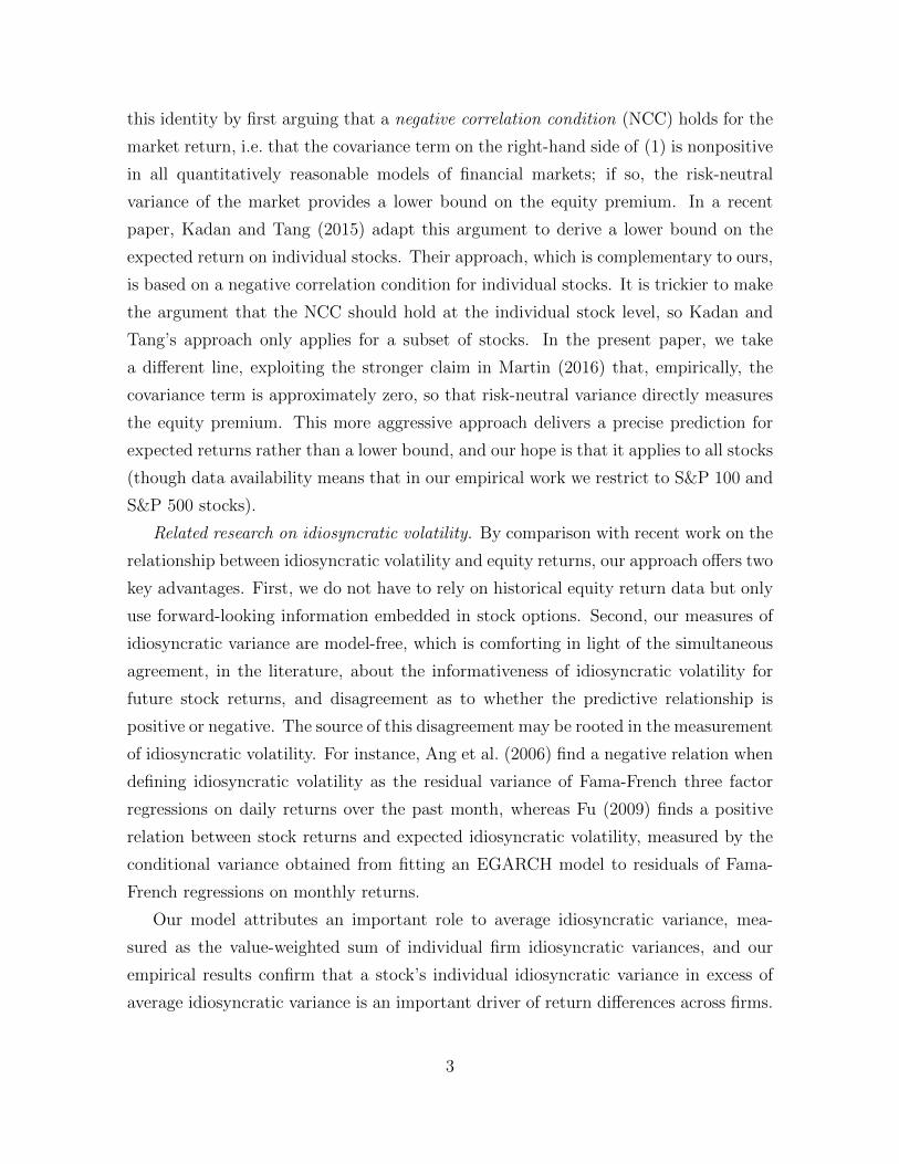
Figure 1: Left: The error, ∆, associated with approximating the geometric meanRi,t+1Rg,t+1 with the arithmetic mean, (R2

i,t+1 +R2g,t+1)/2. R2

i,t+1 and R2g,t+1 lie on the

diameter of a semicircle. Right: Percentage error as a function of Ri,t+1/Rg,t+1.

we ignored the correction term entirely: see Figure 1. Moreover, all this takes place

inside the expectation, so actually all we would need is that Ri,t+1 and Rg,t+1 should

be tolerably close together on (risk-neutral) average.

Returning to equation (5), it follows (using the fact that E∗t Ri,t+1 = Rf,t+1 for any

gross return Ri,t+1) that

EtRi,t+1 −Rf,t+1

Rf,t+1

=1

2var∗t

Ri,t+1

Rf,t+1

+1

2var∗t

Rg,t+1

Rf,t+1

+ ∆i,t (6)

where we define ∆i,t = −12

var∗t [(Ri,t+1 −Rg,t+1) /Rf,t+1]. We have not made any as-

sumptions yet: equation (6) holds as an identity. The term ∆i,t would drop out if

we ignored the distinction between arithmetic and geometric averages. As already

noted, we will not do so, but we will henceforth assume that it can be decomposed

as ∆i,t = αi + λt. (We could have considered other simplifying assumptions on the

structure of ∆i,t—perhaps that ∆i,t = αiλt, for example—but given that we have an

a priori reason to expect that ∆i,t is small, we prefer the econometrically more con-

venient additive formulation.) We can then without further loss of generality assume

that∑

iwi,tαi = 0, where wi,t is the market weight of asset i.

Multiplying equation (6) by wi,t and summing over i, we find that

EtRm,t+1 −Rf,t+1

Rf,t+1

=1

2

∑i

wi,t var∗tRi,t+1

Rf,t+1

+1

2var∗t

Rg,t+1

Rf,t+1

+ λt. (7)

where Rm,t+1 =∑

iwi,tRi,t+1 is the return on the market. Subtracting equation (7)

6

from equation (6) and rearranging, we find that

EtRi,t+1 −Rf,t+1

Rf,t+1

= αi +EtRm,t+1 −Rf,t+1

Rf,t+1

+1

2

(var∗t

Ri,t+1

Rf,t+1

−∑i

wi,t var∗tRi,t+1

Rf,t+1

),

(8)

where∑

iwi,tαi = 0.

It will be convenient to define three different measures of risk-neutral variance:

SVIX2t = var∗t (Rm,t+1/Rf,t+1)

SVIX2i,t = var∗t (Ri,t+1/Rf,t+1) (9)

SVIX2

t =∑i

wi,t SVIX2i,t .

These measures can be computed directly from option prices, as we show in the next

section. The SVIX index was introduced by Martin (2016)—the name echoes the

related VIX index—but the definitions of stock-level SVIXi,t and of SVIXt, which

measures average idiosyncratic volatility, are new to this paper. We note that average

idiosyncratic volatility must exceed market volatility,4 that is, SVIXt > SVIXt.

Introducing these definitions into (8) we arrive at our first, purely relative, predic-

tion about the cross-section of expected returns in excess of the market :

EtRi,t+1 −Rm,t+1

Rf,t+1

= αi +1

2

(SVIX2

i,t−SVIX2

t

)where

∑i

wi,tαi = 0. (10)

We test this prediction by running a panel regression of realized returns-in-excess-

of-the-market of individual stocks i onto stock fixed effects and excess idiosyncratic

variance SVIX2i,t−SVIX

2

t .

In order to answer the question posed in the title of the paper, we need to take

a view on the expected return on the market itself. To do so, we exploit a result of

Martin (2016), who argues that the SVIX index can be used as a forecast of the equity

premium: specifically, that EtRm,t+1 − Rf,t+1 = Rf,t+1 SVIX2t . Substituting this into

4To establish this, we must show that∑i wi,t var∗t Ri,t+1 > var∗t

∑i wi,tRi,t+1; equivalently, that∑

i wi,t E∗t R

2i,t+1 > E∗

t

[(∑i wi,tRi,t+1)

2], or E∗

t

∑i wi,tR

2i,t+1 > E∗

t

[(∑i wi,tRi,t+1)

2]. This follows

since∑i wi,tR

2i,t+1 > (

∑i wi,tRi,t+1)

2by Jensen’s inequality.

7

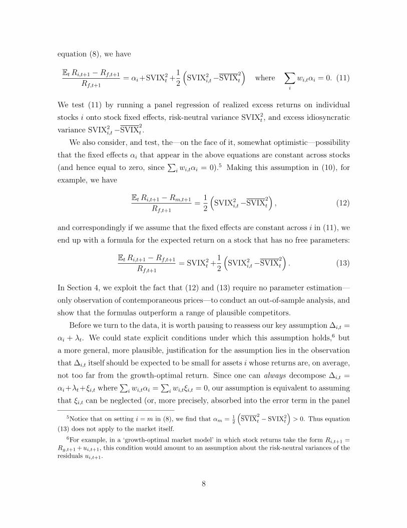
equation (8), we have

EtRi,t+1 −Rf,t+1

Rf,t+1

= αi+SVIX2t +

1

2

(SVIX2

i,t−SVIX2

t

)where

∑i

wi,tαi = 0. (11)

We test (11) by running a panel regression of realized excess returns on individual

stocks i onto stock fixed effects, risk-neutral variance SVIX2t , and excess idiosyncratic

variance SVIX2i,t−SVIX

2

t .

We also consider, and test, the—on the face of it, somewhat optimistic—possibility

that the fixed effects αi that appear in the above equations are constant across stocks

(and hence equal to zero, since∑

iwi,tαi = 0).5 Making this assumption in (10), for

example, we have

EtRi,t+1 −Rm,t+1

Rf,t+1

=1

2

(SVIX2

i,t−SVIX2

t

), (12)

and correspondingly if we assume that the fixed effects are constant across i in (11), we

end up with a formula for the expected return on a stock that has no free parameters:

EtRi,t+1 −Rf,t+1

Rf,t+1

= SVIX2t +

1

2

(SVIX2

i,t−SVIX2

t

). (13)

In Section 4, we exploit the fact that (12) and (13) require no parameter estimation—

only observation of contemporaneous prices—to conduct an out-of-sample analysis, and

show that the formulas outperform a range of plausible competitors.

Before we turn to the data, it is worth pausing to reassess our key assumption ∆i,t =

αi + λt. We could state explicit conditions under which this assumption holds,6 but

a more general, more plausible, justification for the assumption lies in the observation

that ∆i,t itself should be expected to be small for assets i whose returns are, on average,

not too far from the growth-optimal return. Since one can always decompose ∆i,t =

αi+λt+ξi,t where∑

iwi,tαi =∑

iwi,tξi,t = 0, our assumption is equivalent to assuming

that ξi,t can be neglected (or, more precisely, absorbed into the error term in the panel

5Notice that on setting i = m in (8), we find that αm = 12

(SVIX

2

t − SVIX2t

)> 0. Thus equation

(13) does not apply to the market itself.

6For example, in a ‘growth-optimal market model’ in which stock returns take the form Ri,t+1 =Rg,t+1 +ui,t+1, this condition would amount to an assumption about the risk-neutral variances of theresiduals ui,t+1.

8

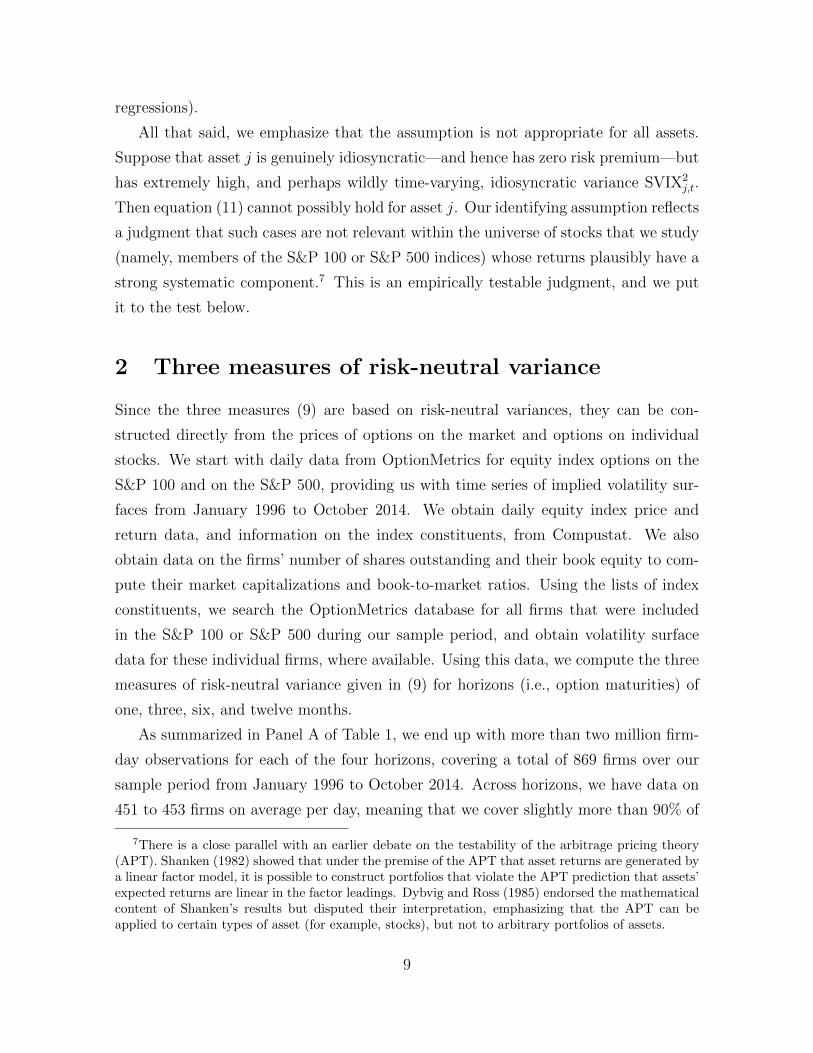
regressions).

All that said, we emphasize that the assumption is not appropriate for all assets.

Suppose that asset j is genuinely idiosyncratic—and hence has zero risk premium—but

has extremely high, and perhaps wildly time-varying, idiosyncratic variance SVIX2j,t.

Then equation (11) cannot possibly hold for asset j. Our identifying assumption reflects

a judgment that such cases are not relevant within the universe of stocks that we study

(namely, members of the S&P 100 or S&P 500 indices) whose returns plausibly have a

strong systematic component.7 This is an empirically testable judgment, and we put

it to the test below.

2 Three measures of risk-neutral variance

Since the three measures (9) are based on risk-neutral variances, they can be con-

structed directly from the prices of options on the market and options on individual

stocks. We start with daily data from OptionMetrics for equity index options on the

S&P 100 and on the S&P 500, providing us with time series of implied volatility sur-

faces from January 1996 to October 2014. We obtain daily equity index price and

return data, and information on the index constituents, from Compustat. We also

obtain data on the firms’ number of shares outstanding and their book equity to com-

pute their market capitalizations and book-to-market ratios. Using the lists of index

constituents, we search the OptionMetrics database for all firms that were included

in the S&P 100 or S&P 500 during our sample period, and obtain volatility surface

data for these individual firms, where available. Using this data, we compute the three

measures of risk-neutral variance given in (9) for horizons (i.e., option maturities) of

one, three, six, and twelve months.

As summarized in Panel A of Table 1, we end up with more than two million firm-

day observations for each of the four horizons, covering a total of 869 firms over our

sample period from January 1996 to October 2014. Across horizons, we have data on

451 to 453 firms on average per day, meaning that we cover slightly more than 90% of

7There is a close parallel with an earlier debate on the testability of the arbitrage pricing theory(APT). Shanken (1982) showed that under the premise of the APT that asset returns are generated bya linear factor model, it is possible to construct portfolios that violate the APT prediction that assets’expected returns are linear in the factor leadings. Dybvig and Ross (1985) endorsed the mathematicalcontent of Shanken’s results but disputed their interpretation, emphasizing that the APT can beapplied to certain types of asset (for example, stocks), but not to arbitrary portfolios of assets.

9

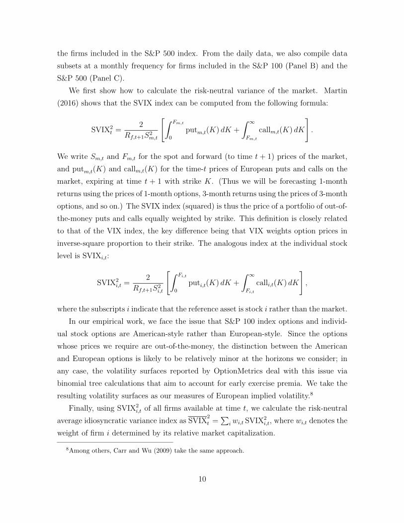
the firms included in the S&P 500 index. From the daily data, we also compile data

subsets at a monthly frequency for firms included in the S&P 100 (Panel B) and the

S&P 500 (Panel C).

We first show how to calculate the risk-neutral variance of the market. Martin

(2016) shows that the SVIX index can be computed from the following formula:

SVIX2t =

2

Rf,t+1S2m,t

[∫ Fm,t

0

putm,t(K) dK +

∫ ∞Fm,t

callm,t(K) dK

].

We write Sm,t and Fm,t for the spot and forward (to time t + 1) prices of the market,

and putm,t(K) and callm,t(K) for the time-t prices of European puts and calls on the

market, expiring at time t + 1 with strike K. (Thus we will be forecasting 1-month

returns using the prices of 1-month options, 3-month returns using the prices of 3-month

options, and so on.) The SVIX index (squared) is thus the price of a portfolio of out-of-

the-money puts and calls equally weighted by strike. This definition is closely related

to that of the VIX index, the key difference being that VIX weights option prices in

inverse-square proportion to their strike. The analogous index at the individual stock

level is SVIXi,t:

SVIX2i,t =

2

Rf,t+1S2i,t

[∫ Fi,t

0

puti,t(K) dK +

∫ ∞Fi,t

calli,t(K) dK

],

where the subscripts i indicate that the reference asset is stock i rather than the market.

In our empirical work, we face the issue that S&P 100 index options and individ-

ual stock options are American-style rather than European-style. Since the options

whose prices we require are out-of-the-money, the distinction between the American

and European options is likely to be relatively minor at the horizons we consider; in

any case, the volatility surfaces reported by OptionMetrics deal with this issue via

binomial tree calculations that aim to account for early exercise premia. We take the

resulting volatility surfaces as our measures of European implied volatility.8

Finally, using SVIX2i,t of all firms available at time t, we calculate the risk-neutral

average idiosyncratic variance index as SVIX2

t =∑

iwi,t SVIX2i,t, where wi,t denotes the

weight of firm i determined by its relative market capitalization.

8Among others, Carr and Wu (2009) take the same approach.

10

Figures 2 and 3 plot the time series of risk-neutral market variance (SVIX2t ) and

average idiosyncratic risk-neutral variance (SVIX2

t ) for the S&P 100 and S&P 500, re-

spectively. The dynamics of SVIX2t and SVIX

2

t are similar for S&P 100 and S&P 500

stocks. As noted in Section 1, SVIX2

t must always be larger than SVIX2t . All the time

series spike dramatically during the financial crisis of 2008. While the average levels of

the SVIX measures are similar across horizons, their volatility is higher at short than

at long horizons. Similarly, the peaks in SVIX2t and SVIX

2

t during the crisis and other

periods of heightened volatility are most pronounced in short-maturity options. An-

other noteworthy feature of the plots is the high level of average idiosyncratic variance,

relative to market variance, over the period from 2000 to 2002.

SVIX2i,t is positively related to CAPM beta and inversely related to firm size, both

on average (Figure 4, Panels A and B) and throughout our sample period (Figure 5,

Panels A and B). In contrast, there is a U-shaped relationship between SVIX2i,t and

book-to-market (Figure 4, Panel C) that reflects an interesting time-series relationship

between book-to-market and SVIX2i,t. While growth and value stocks had similar levels

of (risk-neutral) volatility in periods of low index volatility, value stocks were more

volatile than growth stocks during the recent financial crisis and less volatile from 2000

to 2002 (Figure 5, Panel C). For momentum, we also find that the relation is non-

monotonic on average (Figure 4, Panel D) and that loser stocks exhibited particularly

high SVIX2i,t from the peak of the financial crisis in 2008 to the momentum crash in

early 2009.

3 Testing the model

In this section, we use SVIX2t , SVIX2

i,t, and SVIX2

t to test our theory of expected returns

using full sample information. In the next, we explore the accuracy of our forecasts

out-of-sample.

Before turning to formal tests of our model, we conduct a preliminary exploratory

exercise. Specifically, we ask whether, on time-series average, stocks’ average excess

returns line up with their excess idiosyncratic variances in the manner predicted by

equation (13). To do so, we restrict to firms that were included in the S&P 500

throughout our sample period. For each such firm, we compute time-averaged excess

returns and excess idiosyncratic risk-neutral variance, SVIX2i −SVIX

2. Equation (13)

11

implies that for each percentage point difference in SVIX2i −SVIX

2, we should see half

that percentage point difference in excess returns. The results of this exercise are

shown in Figure 6, which is analogous to the security market line (SML) of the CAPM.

The return horizon matches the maturity of the options used to compute the SVIX-

indices. When we regress average excess returns on 0.5 × (SVIX2i −SVIX

2), we find

slope coefficients of 0.66, 0.85, 1.03, and 1.12 for horizons of one, three, six, and twelve

months, respectively—close to the model-predicted coefficient of one; the regression

intercept reflects the average excess return of the market. The R-squared of these

regressions is in the range from 0.11 to 0.20, suggesting that SVIX2i −SVIX

2accounts

for a fair amount of variation across firms’ average excess returns. The figures also

show 3x3 portfolios sorted on size and book-to-market (B/M), indicated by triangles.

Encouragingly, these portfolios line up quite well with our model.

Moreover, we use all firms available in our data (i.e. we lift the requirement of full

sample period coverage) to conduct conventional portfolio sorts based on firms’ relative

idiosyncratic variance, CAPM beta, size, B/M ratios, and momentum. Figures 7 and

8 show that average portfolio returns in excess of the market are broadly increasing in

portfolios’ average idiosyncratic volatility relative to aggregate idiosyncratic volatility,

and that SVIX2i −SVIX

2captures a sizeable fraction of the cross-sectional variation in

returns. We explore the interaction between model-implied return forecasts and firm

characteristics in more detail below.

To test our model more formally, we now explore the conditional relation of indi-

vidual stock excess returns to risk-neutral index variance (SVIX2t ) and stocks’ excess

idiosyncratic risk-neutral variance (SVIX2i,t−SVIX

2

t ). At a given point in time t, our

sample includes all firms that are time-t constituents of the index that serves as a proxy

for the market. Using monthly data, we evaluate return horizons of one, three, six,

and twelve months by estimating the pooled regression

Ri,t+1 −Rf,t+1

Rf,t+1

= α + β SVIX2t +γ

(SVIX2

i,t−SVIX2

t

)+ εi,t+1, (14)

which constitutes a test of our formula (13) for the expected return on a stock; our

theory implies that α = 0, β = 1 and γ = 1/2. We test the prediction (11) by running

12

a panel regression with firm fixed effects

Ri,t+1 −Rf,t+1

Rf,t+1

= αi + β SVIX2t +γ

(SVIX2

i,t−SVIX2

t

)+ εi,t+1. (15)

In this form, our theory continues to imply that β = 1 and γ = 1/2, but now it allows

the fixed effects αi to vary across stocks, subject to the constraint that∑

iwi,tαi = 0.

We compute standard errors via a block-bootstrap procedure that accounts for time-

series and cross-sectional dependencies in our data.9 We present the regression results

for S&P 100 firms in Table 2 and for S&P 500 firms in Table 3.

We start with the pooled regression results for S&P 100 firms in Panel A of Table 2.

We conduct a Wald test for the joint hypothesis that α = 0, β = 1, and γ = 0.5, using

bootstrapped standard errors. The headline result is that, with p-values ranging from

0.48 to 0.66, we do not reject our model at any horizon. By contrast, we can reject

the joint hypothesis that β = 0 and γ = 0 with moderate confidence for six- and

twelve-month returns (p-values of 0.071 and 0.043, respectively), though not at shorter

horizons. The point estimates of β are 0.027, 1.094, 2.286, and 1.966 for horizons

of one, three, six, and twelve months, respectively. These numbers are consistent

with our model, but the coefficients are imprecisely estimated so are not (individually)

significantly different from zero. The point estimates of γ are 0.340, 0.397, 0.664, and

0.840 at the four horizons. At horizons of six and twelve months, these estimates are

(individually) significantly different from zero, indicating a strong, positive relation

between firms’ equity returns and their excess idiosyncratic variance.

Accounting for firm fixed effects (in Panel B) does not change this conclusion, and

encouragingly the coefficient estimates remain reasonably stable. A Wald test of the

joint null hypothesis that Σiwi,tαi = 0, β = 1, and γ = 0.5 does not reject the model (p-

values between 0.11 and 0.42), and we can strongly reject the joint null that β = γ = 0

for horizons of six and twelve months (p-values of 0.020 and 0.000, respectively). The

9Petersen (2009) provides an extensive discussion of how cross-sectional and time-series depen-dencies may bias standard errors in OLS regressions and suggests using two-way clustered standarderrors. We take an more conservative approach for two reasons. First, for return horizons exceedingone month, our monthly return data uses overlapping observations. Second, our data is characterizedby very high but less than perfect coverage of index constituent firms, due to limited availability ofoptions information. We therefore use an overlapping block resampling scheme to handle serial corre-lation and heteroskedasticity, and for every bootstrap iteration, we randomly choose which constituentfirms to include in the bootstrap sample. For more details on block bootstrap procedures, see, e.g.,Kuensch (1989), Hall et al. (1995), Politis and White (2004), and Patton et al. (2009).

13

β estimates are little changed compared to the pooled regressions. The γ estimates

are somewhat higher—from 0.533 to 1.230—and more significant with bootstrap t-

statistics of 1.65, 2.66, and 3.93 for horizons of three, six, and twelve months. We

also find, in line with our theory, that the value-weighted sum of firm fixed effects,∑iwi,tαi, is not statistically different from zero.10

We find similar results for S&P 500 firms (Table 3). In the pooled regression

(Panel A), we do not reject the joint null that α = 0, β = 1, and γ = 0.5 at any

horizon (p-values between 0.154 and 0.185); and we can cautiously reject the joint null

that β = 0 and γ = 0 at horizons of six and twelve months (p-values of 0.072 and

0.092). The statistical results are more clear-cut when we take firm fixed effects into

account, in Panel B. Again, we do not reject the joint null hypothesis implied by our

model at any horizon, but can strongly reject the null that β = γ = 0 at horizons of

six and twelve months (p-values of 0.023 and 0.008).

To focus on the purely cross-sectional predictions of our framework, we test the

prediction of equation (12) by running the regression

Ri,t+1 −Rm,t+1

Rf,t+1

= α + γ(

SVIX2i,t−SVIX

2

t

)+ εi,t+1, (16)

and the less optimistic prediction (10) by allowing for stock fixed effects,

Ri,t+1 −Rm,t+1

Rf,t+1

= αi + γ(

SVIX2i,t−SVIX

2

t

)+ εi,t+1. (17)

The theoretical prediction is then that α = 0 and γ = 1/2 in (16), or that∑

iwi,tαi = 0

and γ = 1/2 in (17). In this form, we avoid relying on the finding of Martin (2016)

that the equity premium can be proxied by Rf,t+1 SVIX2t , though of course we can

only make a relative statement about the cross-section of expected returns. In our

empirical analysis we compute Rm,t+1 as the return on the value-weighted portfolio of

all index constituent firms included in our sample at time t. Tables 4 and 5 report

the regression results for S&P 100 and S&P 500 firms. The results are consistent with

the preceding evidence. For the pooled regressions, the estimated intercepts α are

statistically insignificant, while the estimates of γ are significant at horizons of six and

10The estimate reported for Σiwi,tαi is the time-series average of the value-weighted sum of firmfixed effects computed every period in our sample. The t-statistic is based on the distribution of thetime-series average of Σiwi,tαi across bootstrap iterations.

14

twelve months. The Wald tests of the joint hypothesis that α = 0 and γ = 0.5 do not

reject our model (p-values between 0.368 and 0.801). Accounting for firm fixed effects,

the significance of the γ-estimate becomes more pronounced across return horizons,

with p-values of the null hypothesis γ = 0 being 0.10 or less even at the very short

horizons. We also find that the value-weighted sum of firm fixed effects is statistically

different from zero, though the estimates are fairly small in economic terms—and,

reassuringly, we will see in the next section that our model performs well when we

drop firm fixed effects entirely, as we do in our out-of-sample analysis.

Lastly, we test our theory on the expected returns of portfolios sorted by CAPM

beta, size, book-to-market, and momentum. At the end of every month, we sort S&P

100 (S&P 500) firms into decile (25) portfolios and compute the portfolios’ (equally-

weighted) returns in excess of the market as well as the portfolios’ idiosyncratic variance

in excess of aggregate idiosyncratic variance. Using these portfolio series, we run the

regressions specified in equations (16) and (17) and present results for S&P 100 and

S&P 500 stock portfolios in Tables 6 and 7, respectively. For both indices we find

that regression intercepts and fixed effects are insignificant and that estimates of γ are

positive across all portfolios. For size-sorted portfolios, we find that estimates of γ

significantly exceed the theoretical value of 0.5 and that the joint hypothesis tests, as a

consequence, reject the model. In other words, excess idiosyncratic volatility forecasts

returns even more strongly than our theory predicts. When we sort portfolios by beta,

book-to-market, and momentum, the γ-estimates are not statistically different from the

theoretical value of 0.5 and the joint hypothesis tests never reject our model. Moreover,

for portfolios of S&P 100 stocks we reject γ = 0 for all firm characteristics.

Taken together, the above results provide supportive evidence in favor of our the-

oretical relationship between expected returns, index risk-neutral variance, and excess

idiosyncratic variance.

4 Out-of-sample analysis

We now turn to see how the model performs in an out-of-sample exercise. We compute

expected returns on stocks using the SVIX2t , SVIX2

i,t, and SVIX2

t series by imposing

the parameter values β = 1, γ = 1/2 dictated by our theory. Since we want a pure

out-of-sample test in which no parameters are estimated from the data, we impose our

15

more optimistic model (13) without fixed effects—that is, we compute the conditional

expectation for the excess return on stock i as

EtRi,t+1 −Rf,t+1

Rf,t+1

= SVIX2t +

1

2

(SVIX2

i,t−SVIX2

t

).

Figure 9 shows the time-series of real-time expected excess returns implied by this

formula for some leading tech stocks (IBM, Microsoft, and Apple) and financial stocks

(Citigroup, JP Morgan, and Bank of America). According to our formula, all the firms

had very high risk premia during the crisis of 2008, but the effect was particularly

extreme for the financial firms. Earlier in the sample, the risk premia of IBM and

Microsoft were high from 1996 to early 1999, low during 2001, and high again around

the market lows of late 2002, while the risk premium on Apple was high for most of

the sample pre-2002.

Finally, we focus on the cross-sectional dimension of firms’ equity returns by com-

puting forecasts of expected returns in excess of the market, as in (12):

EtRi,t+1 −Rm,t+1

Rf,t+1

=1

2

(SVIX2

i,t−SVIX2

t

).

Figure 10 contrasts expected excess returns and returns in excess of the market for

Apple and JP Morgan to illustrate that high expected returns as (judge by an individual

firm’s time series) do not necessarily coincide with high expected returns in excess of

the market, i.e. in the cross-section of firms. For both firms expected returns exhibit

a spike during the crisis of 2008, but for Apple this spike coincides with the lowest

expected return in excess of the market over its sample history.

4.1 Statistical forecast accuracy

Using the model-implied conditional expectations from equation (13), we now assess

the statistical forecast accuracy of our model for individual firm stock returns relative

to competing benchmark forecasts.

What are the natural competitor benchmarks? One possibility is to give up on

trying to make differential predictions across stocks, and simply to use a forecast of

the expected return on the market as a forecast for each individual stock. Following

Goyal and Welch (2008) and Campbell and Thompson (2008), we use the market’s

16

historical average excess return as a benchmark forecast, where we choose the S&P

500 (S&P500t) and the CRSP value-weighted index (CRSPt) as proxies for the market.

Additionally, we use the risk-neutral market variance (SVIX2t , computed from S&P

500 index options) as a benchmark forecast, which Martin (2016) shows to provide

predictive ability for the market return beyond the historical average.

More ambitious competitor models would seek to provide differential forecasts of

individual firm stock returns, as we do. One natural thought is to use historical average

of firms’ stock excess returns (RXi,t). Another is to estimate firms’ conditional CAPM

betas from historical return data (following Frazzini and Pedersen, 2014) and combine

the beta estimates with the aforementioned market premium predictions. Finally,

we follow Kadan and Tang (2015) by using firms’ idiosyncratic variances (SVIX2i,t)

to forecast stock returns. While in our model SVIX2i,t is only one component of the

expected return, Kadan and Tang argue that SVIX2i,t can, under certain conditions,

be viewed as a lower bound on expected stock returns and they find that it conveys

information for subsequent stock returns.

To compare the forecast accuracy of the model to that of the benchmarks, we

compute an out-of-sample R-squared similar to that of Goyal and Welch (2008). We

define

R2OS = 1−

∑i

∑t FE

2M∑

i

∑t FE

2B

,

where FEM and FEB denote the forecast errors from our model and a benchmark

prediction, respectively. The results in Panel A of Table 8 show that R2OS-values are

generally positive and increasing with forecast horizon.11 At the one-year horizon, R2OS-

values are in the range from 1.7% to 3.8% relative to the market forecasts and compared

to the individual stock return forecasts, except for the historical average firm stock

return which performs much worse than all other predictors.12 These results confirm

11The R2OS results are based on expected excess returns defined as EtRi,t+1 − Rf,t+1, i.e. we

multiply the left and the right side of equation (13) by Rf,t+1. We do so because the benchmarkforecasts of excess returns are generally computed from excess returns Ri,t+1 −Rf,t+1.

12As mentioned above, using the historical average of a firm’s stock was motivated by the usage ofanalogous predictors for market returns. But for individual firms, short historical return series maynot be representative of future returns; consider for instance tech firms that were relatively young atthe peak of the dotcom bubble and therefore had an extremely high historical average return overtheir short histories. In these cases, employing the historical average as a predictor may lead to largeforecast errors for subsequent returns. Examples like these further emphasize the usefulness of ourapproach, which does not rely on historical data and only requires option prices at time t.

17

that our model forecasts convey information for future stock returns and outperform

the competitor benchmarks described above.

We also compute R2OS for expected returns in excess of the market as defined in

equation (12) and report the results in Panel B. We adjusted the conditional CAPM

predictions accordingly (i.e. we multiply the market premium forecast by beta minus 1)

and add a ‘random walk’ forecast of zero. Focussing on the cross-sectional dimension of

firms’ equity returns, net of (noisy) market return forecasts, strengthens the evidence

that our model forecasts are superior to the benchmarks. All R2OS-estimates are positive

and increase with forecast horizon. At the one-year horizon, R2OS compared to the zero

return prediction is 3.10% and the R2OS-values relative to the CAPM forecasts are

similarly in a range between 3.11% and 3.36%. Our model easily beats the SVIX2i,t-

forecast with a R2OS of 7.18%, highlighting that a firm’s expected excess return is not

only related to its own idiosyncratic variance but also to the market-wide average

idiosyncratic volatility across all firms. These results also confirm that setting γ = 0.5

is useful for out-of-sample purposes.

4.2 Economic value of model forecasts

To assess whether conditioning on stock return forecasts from our model generates

economic value for investors, we now compare the performance of a portfolio with

weights determined by model forecasts to a value-weighted portfolio and to an equally-

weighted portfolio. The value-weighted portfolio serves as a natural benchmark because

it mimics the market.13 The equally-weighted portfolio has proven in previous research

to be a tough benchmark to beat (see, e.g. DeMiguel et al., 2009) and therefore serves as

a natural competitor as well. Using both the equally- and the value-weighted portfolios

as benchmarks takes size effects into account to some extent, but we also investigate

how the performance of our portfolios relates to firm size and book-to-market in more

detail below.

Our results above suggest that the model forecasts expected excess returns accu-

rately out-of-sample. Since it is not possible to estimate an options-implied covariance

13More precisely, the value-weighted portfolio mimics the market to the extent that constituentfirms are included in the sample at time t, which is subject to availability of equity options data. Inour analysis of out-of-sample economic value, we cover more than 90% of S&P 500 firms on average.Over our full sample period the return on the value-weighted portfolio is somewhat higher than thatof the S&P 500 index, but the monthly excess return correlation exceeds 0.999.

18

matrix of individual stocks (due to the lack of derivatives that trade on pairs of stocks),

we apply a portfolio approach that only requires the expected return as a signal for the

investment decision. More specifically, we draw on the idea of Asness et al. (2013) and

construct portfolios based on the ranks of firms’ expected returns, where we determine

the portfolio weight of firm i for the period from t to t+ 1 as

wXSi,t =rank[EtRi,t+1]

θ∑i rank[EtRi,t+1]θ

, (18)

where θ > 0 controls the aggressiveness of the strategy. This methodology assigns

weights that increase with expected excess returns, does not allow for short positions,

and ensures that the investor is fully invested in the stock market, i.e.∑

iwXSi,t = 1.

We do not allow short positions because this would impede a comparison with the

value- and equally-weighted benchmark portfolios, which are by definition long-only

portfolios. Moreover, using rank-weights ensures that the portfolio is well-diversified

and avoids extreme portfolio positions. By increasing the aggressiveness parameter θ,

the relative overweighting (underweighting) of firms with high (low) expected returns

becomes more pronounced but the tilting from equal weights remains moderate.14

To evaluate the portfolio relative to the benchmarks, we compute returns, sample

moments, Sharpe ratios, and the performance fee as defined by Fleming et al. (2001).

For a given relative risk aversion ρ, the performance fee (Φ) quantifies the premium that

a risk-averse investor would be willing to pay to switch from the benchmark investment

(B) to the portfolio conditioning on the forecasts from our model (M). Specifically,

Φ is computed as a fraction of initial wealth (W0) such that two competing portfolio

strategies achieve equal average utility. Denoting the gross portfolio return of portfolio

k ∈ {B,M} by Rk,t+1, we compute the average realized utility, U ({Rk,t+1}), as

U ({Rk,t+1}) = W0

(T−1∑t=0

Rk,t+1 −ρ

2(1 + ρ)R2k,t+1

)14For θ = 0, the strategy corresponds to the equally-weighted portfolio benchmark. In our empirical

analysis, we set θ = 1 or θ = 2 which leads to over- or underweighting of stocks relative to the naivebenchmark but avoids extreme positions and ensures that the portfolio is well diversified. For 500stocks, a naive strategy allocates a 0.2%-weight to each asset in the portfolio; the maximum rankweights assigned to a single stock is 0.399% for θ = 1 and 0.598% when setting θ = 2.

19

and estimate the performance fee as the value Φ that satisfies

U ({RM,t+1 − Φ}) = U ({RB,t+1}) .

We start by considering an investor who rebalances her portfolio at the end of

every month. She may either invest in the market by choosing the value-weighted

portfolio or the equally-weighted portfolio, or use the model forecasts to determine the

portfolio weights according to equation (18) where we set θ = 1. Table 9 compares

the performance of these three alternatives. The forecast-based portfolios generate

annualized excess returns between 10.48% and 11.45% with associated Sharpe ratios

between 0.48 and 0.53, where excess returns and Sharpe ratios moderately increase

with the SVIX-horizon used in the forecast.

The model-based portfolios dominate the value-weighted portfolios in terms of

Sharpe ratios and skewness properties such that investors would be willing to pay

a sizeable fee to switch from the benchmark to the model portfolios, where the fee-

estimate Φ depends on the investor’s relative risk aversion. Setting ρ between one and

ten, we find that the annual performance fee is in the range of 2.54% to 4.44%. When

we compare the model portfolio to the naive strategy, the Φ-estimates are positive

as well, albeit at a lower level. The equally-weighted portfolios have slightly higher

Sharpe ratios than the model portfolios but less favorable skewness properties such

that investors would be willing to pay performance fees between 0.27% to 1.38% per

year to switch to the model portfolio.

A major advantage of our approach is that it allows the investor to update her

expectations about every single firm in real-time. Table 10 presents performance results

when the investor rebalances her portfolios at the end of every day. Allowing for more

timely portfolio adjustments, we find that the model portfolios perform very similarly

for all variance-horizons used in the forecast. Daily rebalancing based on the model

forecasts widens the gap between model and value-weighted portfolio Sharpe ratios, and

the Sharpe ratios of the model portfolios are similar to those of the naive portfolios.

Moreover, conditioning on SVIX-information leads to less negative return skewness

relative to the benchmark investments. The Φ-estimates increase compared to the

monthly rebalancing results, with investors willing to pay performance fees in the

range between 3.85% to 4.60% compared to the value-weighted portfolios and 0.93%

to 1.61% compared to the equally-weighted portfolios.

20

To provide further evidence that SVIX-based forecasts generate economic value, we

now increase the aggressiveness of the strategy by setting θ = 2. The results in Table

11 show that putting more emphasis on the forecast when determining the portfolio

weights leads to further utility gains for investors. The estimated performance fee for

investing in the model instead of the market portfolio is between 4.14% and 5.41% per

year. Comparing the model to the naive portfolio, we find that estimates of Φ are in

the range from 1.23% to 2.42% per year.

The above results indicate that option prices contain valuable information in a

manner that is consistent with our theoretical model. Figure 11 illustrates the dynamics

of the model and the benchmark portfolios by plotting the cumulative returns of daily

rebalanced portfolios using forecasts based on SVIX-horizons of one month and one

year.

We repeat the economic value analysis to gauge the interaction between our model

forecasts, firm size, and book-to-market for the performance of portfolio strategies.

The results reported below use forecasts based on the one-year SVIX horizon but

our conclusion that conditioning on model forecasts generates economic value remains

unchanged when using shorter horizons. Starting with portfolios that are rebalanced

at a monthly frequency and setting θ = 1, Table 12 shows that the model generates

higher utility gains for investments in small firms than in big firms. Similarly, investors

would be willing to pay a higher fee to switch from the value- or equally-weighted

benchmark to the model-portfolio when investing in value stocks compared to growth

stocks. Allowing the investor to adjust her portfolio at a daily frequency and to trade

more aggressively on the model signals (by setting θ = 2), the estimated performance

fees increase in all size and book-to-market portfolios, where, again, the economic value

attainable is larger for small caps and value stocks. Figure 12 illustrates the time-series

dynamics of the portfolio strategies by plotting their cumulative returns.

5 Further results and robustness checks

We now briefly summarize the findings of additional empirical exercises that corrobo-

rate our conclusions; we report these results in detail in the separate Internet Appendix.

In the analysis above, we report results for the link between firm characteristics

(beta, size, book-to-market, and momentum) and SVIX for horizons of one year. Fig-

21

ures IA.1 and IA.2 show that these links are very similar for a horizon of one month.

Second, we complement the regression analysis of expected returns in excess of the

market for characteristic-sorted portfolios with regressions of their expected excess re-

turns; see Tables IA.1 and IA.2. We take a closer look at the interaction of size and

value by exploring double-sorted portfolios and present results for the SVIX-time series

properties of size/book-to-market portfolios (Figure IA.3), their average expected re-

turns in excess of the market (Figure IA.4), and the out-of-sample performance of our

asset allocation exercise in double-sorted size/book-to-market portfolios (Table IA.3

and Figure IA.5)

Finally, we present additional examples of real-time expected returns for individual

firms. Using data for Ford and General Motors, Figure IA.6 plots expected excess

returns and expected returns in excess of the market, which both look very similar

because the market return-adjustment mainly affects the return level. The picture

looks different for Coca Cola and Pepsi in Figure IA.7. During the crisis of 2008, both

firms had expected returns that were unusually high relative to the riskless rate, but

unusually low relative to the market.

6 Conclusions

This paper has presented new theoretical and empirical results on the cross-section of

expected stock returns. We would like to think that our approach to this classic topic

is idiosyncratic in more than one sense.

Our empirical work is tightly constrained by our theory. In sharp contrast with

the factor model approach to the cross-section—which has both the advantage and

the disadvantage of imposing very little structure, and therefore says ex ante little

about the anticipated signs, and nothing about the sizes, of coefficient estimates—we

make specific predictions both for the signs and sizes of coefficients, and test these

numerical predictions in the data. In this dimension, a better comparison is with

the CAPM, which makes the quantitative prediction that the slope of the security

market line should equal the market risk premium. But (setting aside the fact that it

makes no prediction for the market risk premium) even the CAPM requires betas to

be estimated if this prediction is to be tested. At times when markets are turbulent, it

is far from clear that historical betas provide robust measures of the idealized forward-

22

looking betas called for by the theory; and if the goal is to forecast returns over, say,

a one-year horizon, one cannot respond to this critique by taking refuge in the last

five minutes of high-frequency data. In contrast, our predictive variables—as option

prices—are observable in real time and inherently forward-looking.

Our empirical results are surprisingly supportive of our theory, particularly over

six- and twelve-month horizons. We test the model with and without fixed effects;

using returns in excess of the riskless rate (to answer the question posed in the title)

and in excess of the market (to isolate the cross-sectional predictions and differentiate

our findings from those of Martin (2016)); and for S&P 100 and S&P 500 stocks. At

six- and twelve-month horizons we can reject the null of no predictability with some

confidence, whereas we do not reject our model—and find reasonable stable coefficient

estimates—in most of the specifications. We achieve all this despite the fact that our

empirical work takes place at the individual stock, rather than at the portfolio, level.

We try to find evidence against our model by forming portfolios sorted on four

dimensions known to be problematic for previous generations of asset-pricing models.

The model does a good job of accounting for realized returns on portfolios sorted on

beta, book-to-market, and momentum. When we sort on size, however, we find that

the sensitivity of portfolio returns to idiosyncratic volatility has the ‘right’ sign but is

even stronger than predicted by our framework, and we are able to reject the model.

One of the strengths of our framework is that the coefficients in our formula for

the expected return on a stock emerge from the theory. Implementing this formula

requires us only to observe certain option prices in the market; no estimation is required.

Our approach is therefore not subject to the critique of Goyal and Welch (2008).

We compare the out-of-sample performance of the formula to a range of competitor

predictors of stock returns, and show that it outperforms them all. Finally, we show

how to use our forecasts to generate trading strategies, and show that the resulting

strategies perform well.

Our results point toward a qualitatively and quantitatively new view of expected

returns. Most obviously, our approach implies that expected returns are extremely

volatile across stocks and over time. To take one example, expected returns on some

major financial stocks were astonishingly high in the depths of the 2008–9 crisis: on

our view, the annual expected return on Bank of America peaked above 80%, while

that of Citigroup rose above 100%.

23

References

An, B.-J., Ang, A., Bali, T. G., and Cakici, N. (2014). The joint cross section of stocksand options. The Journal of Finance, 69(5):2279–2337.

Ang, A., Hodrick, R. J., Xing, Y., and Zhang, X. (2006). The cross-section of volatilityand expected returns. The Journal of Finance, 61:259–299.

Asness, C. S., Moskowitz, T. J., and Pedersen, L. H. (2013). Value and momentumeverywhere. Journal of Finance, 68:929–985.

Buss, A. and Vilkov, G. (2012). Measuring equity risk with option-implied correlations.Review of Financial Studies, 25(10):3113–3140.

Campbell, J. Y. and Thompson, S. B. (2008). Predicting excess stock returns out ofsample: Can anything beat the historical average? Review of Financial Studies,21:1509–1531.

Carr, P. and Wu, L. (2009). Variance risk premiums. Review of Financial Studies,22(3):1311 – 1341.

Christoffersen, P., Fournier, M., and Jacobs, K. (2015). The factor structure in equityoptions. Rotman School of Management Working Paper.

Cochrane, J. (2005). Asset Pricing. Princeton University Press, revised edition.

Conrad, J., Dittmar, R., and Ghysels, E. (2013). Ex ante skewness and expected stockreturns. Journal of Finance, 68:85–124.

DeMiguel, V., Garlappi, L., and Uppal, R. (2009). Optimal versus naive diversifica-tion: How inefficient is the 1/n portfolio strategy? Review of Financial Studies,22(5):1915–1953.

Driessen, J., Maenhout, P., and Vilkov, G. (2009). The price of correlation risk: Evi-dence from equity options. Journal of Finance, 64:1377–1406.

Dybvig, P. H. and Ross, S. A. (1985). Yes, the APT is testable. The Journal of Finance,40(4):1173–1188.

Fleming, J., Kirby, C., and Ostdiek, B. (2001). The economic value of volatility timing.Journal of Finance, 56(1):329–352.

Frazzini, A. and Pedersen, L. H. (2014). Betting against beta. Journal of FinancialEconomics, 111(1):1–25.

Fu, F. (2009). Idiosyncratic risk and the cross-section of expected stock returns. Journalof Financial Economics, 91(1):24–37.

24

Goyal, A. and Welch, I. (2008). A comprehensive look at the empirical performance ofequity premium prediction. Review of Financial Studies, 21:1455–1508.

Hall, P., Horowitz, J., and Jing, B. (1995). On blocking rules for the bootstrap withdependent data. Biometrika, 82:561–574.

Hansen, L. P. and Richard, S. F. (1987). The role of conditioning information in de-ducing testable restrictions implied by dynamic asset pricing models. Econometrica,55(3):587–613.

Herskovic, B., Kelly, B., Lustig, H., and Nieuwerburgh, S. V. (2016). The commonfactor in idiosyncratic volatility: Quantitative asset pricing implications. Journal ofFinancial Economics, 119(2):249–283.

Kadan, O. and Tang, X. (2015). A bound on expected stock returns. Working paper,Washington University in St. Louis.

Kuensch, H. (1989). The jacknife and the bootstrap for general stationary observations.Annals of Statistics, 17:1217–1241.

Long, J. B. (1990). The numeraire portfolio. Journal of Financial Economics, 26:29–69.

Martin, I. (2016). What is the expected return on the market? Working paper, LondonSchool of Economics.

Patton, A., Politis, D., and White, H. (2009). Correction to “automatic block-lengthselection for dependent bootstrap”. Econometric Reviews, 28:372–375.

Petersen, M. A. (2009). Estimating standard errors in finance panel data sets: Com-paring approaches. Review of Financial Studies, 22(1):435–480.

Politis, D. and White, H. (2004). Automatic block-length selection for dependentbootstrap. Econometric Reviews, 23:53–70.

Roll, R. (1973). Evidence on the “growth-optimum” model. Journal of Finance,28(3):551–566.

Shanken, J. (1982). The arbitrage pricing theory: Is it testable? The Journal ofFinance, 37(5):1129–1140.

25

Table 1: Sample data

This Table summarizes the data used in the empirical analysis. We search the OptionMetrics database for all firmshat have been included in the S&P 100 or S&P 500 during the sample period from January 1996 to October 2014and obtain all available volatility surface data. Panel A summarizes the number of total observations, the numberof unique days and unique firms in our sample, as well as the average number of firms for which options data isavailable per day. For some econometric analysis, we also compile data subsets at a monthly frequency for firmsincluded in the S&P 100 (summarized in Panel B) and the S&P 500 (Panel C).

Panel A. Daily data

Horizon 30 days 91 days 182 days 365 days

Observations 2,116,480 2,116,073 2,114,678 2,107,484

Sample days 4,675 4,675 4,675 4,675

Sample firms 869 861 855 825

Average firms/day 453 453 452 451

Panel B. Monthly data for S&P 100 firms


Observations 21,235 20,847 20,269 19,121

Sample months 224 222 219 213

Sample firms 177 176 176 171

Average firms/month 95 94 93 90

Panel C. Monthly data for S&P 500 firms


Observations 102,601 100,593 97,629 91,815

Sample months 224 222 219 213

Sample firms 877 869 863 832

Average firms/month 458 453 446 431

26

Table 2: Expected excess returns of S&P 100 firms

This Table presents results from regressing equity excess returns of S&P 100 firms on the risk-neutral varianceof the market variance (SVIX2

t ) and the stock’s idiosyncratic risk-neutral variance measured relative to average

idiosyncratic risk-neutral variance(

SVIX2i,t−SVIX

2

t

). The data is monthly from January 1996 to October 2014.

The column labels indicate the return horizons ranging from one month to one year. The return horizons match

the maturities of the options used to compute SVIX2t , SVIX2

i,t, and SVIX2

t . Panel A reports estimates of the pooledregression specified in equation (14),

Ri,t+1 −Rf,t+1

Rf,t+1= α+ β SVIX2

t +γ(

SVIX2i,t−SVIX

2

t

)+ εi,t+1.

Panel B reports results for the panel regression with firm fixed effects, specified in equation (15),

Ri,t+1 −Rf,t+1

Rf,t+1= αi + β SVIX2

t +γ(

SVIX2i,t−SVIX

2

t

)+ εi,t+1,

where∑i wi,tαi reports the time-series average of the value-weighted sum of firm fixed effects. Values in square

brackets are t-statistics based on standard errors from a block bootstrap procedure. In both panels, the last tworows report p-values of Wald tests on joint parameter significance, testing whether the data rejects the parametervalues implied by our theory (zero intercept, β = 1 and γ = 0.5) and whether β and γ are jointly zero, respectively.The ‘theory adj-R2 (%)’ reports the adjusted-R2 obtained when fixing the parameters at their theoretical values.


Panel A. Pooled regressions

α 0.074 0.035 -0.009 0.001

[1.16] [0.47] [-0.17] [0.01]

β 0.027 1.094 2.286 1.966

[0.01] [0.48] [1.56] [1.40]

γ 0.340 0.397 0.664 0.840

[1.07] [1.30] [2.05] [2.45]

Pooled adj-R2 (%) 0.162 0.796 3.668 6.511

H0 : α = 0, β = 1, γ = 0.5 0.484 0.601 0.655 0.560

H0 : β = γ = 0 0.529 0.428 0.071 0.043

Theory adj-R2 (%) -0.053 0.442 2.461 3.975

Panel B. Firm fixed-effects regressions∑i wiαi 0.087 0.050 0.008 0.018

[1.40] [0.70] [0.15] [0.28]

β -0.014 1.020 2.174 1.802

[-0.01] [0.44] [1.52] [1.36]

γ 0.533 0.614 0.977 1.230

[1.46] [1.65] [2.66] [3.93]

Panel adj-R2 (%) 1.000 4.429 11.439 20.134

H0 :∑i wiαi = 0, β = 1, γ = 0.5 0.296 0.415 0.383 0.106

H0 : β = γ = 0 0.297 0.251 0.020 0.000

27

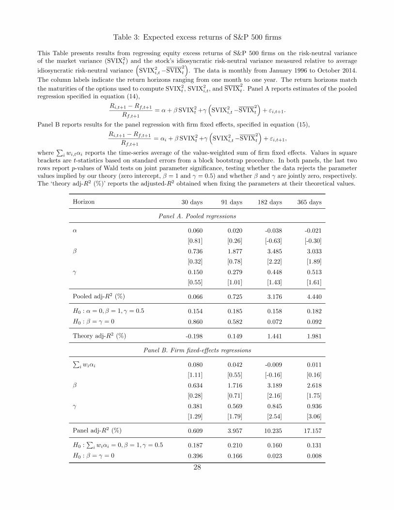
Table 3: Expected excess returns of S&P 500 firms

This Table presents results from regressing equity excess returns of S&P 500 firms on the risk-neutral varianceof the market variance (SVIX2

t ) and the stock’s idiosyncratic risk-neutral variance measured relative to average


SVIX2i,t−SVIX

2

t

). The data is monthly from January 1996 to October 2014.

The column labels indicate the return horizons ranging from one month to one year. The return horizons match

the maturities of the options used to compute SVIX2t , SVIX2

i,t, and SVIX2

t . Panel A reports estimates of the pooledregression specified in equation (14),

Ri,t+1 −Rf,t+1


t +γ(

SVIX2i,t−SVIX

2

t

)+ εi,t+1.

Panel B reports results for the panel regression with firm fixed effects, specified in equation (15),

Ri,t+1 −Rf,t+1


t +γ(

SVIX2i,t−SVIX

2

t

)+ εi,t+1,

where∑i wi,tαi reports the time-series average of the value-weighted sum of firm fixed effects. Values in square

brackets are t-statistics based on standard errors from a block bootstrap procedure. In both panels, the last tworows report p-values of Wald tests on joint parameter significance, testing whether the data rejects the parametervalues implied by our theory (zero intercept, β = 1 and γ = 0.5) and whether β and γ are jointly zero, respectively.The ‘theory adj-R2 (%)’ reports the adjusted-R2 obtained when fixing the parameters at their theoretical values.



α 0.060 0.020 -0.038 -0.021

[0.81] [0.26] [-0.63] [-0.30]

β 0.736 1.877 3.485 3.033

[0.32] [0.78] [2.22] [1.89]

γ 0.150 0.279 0.448 0.513

[0.55] [1.01] [1.43] [1.61]

Pooled adj-R2 (%) 0.066 0.725 3.176 4.440

H0 : α = 0, β = 1, γ = 0.5 0.154 0.185 0.158 0.182

H0 : β = γ = 0 0.860 0.582 0.072 0.092

Theory adj-R2 (%) -0.198 0.149 1.441 1.981

Panel B. Firm fixed-effects regressions∑i wiαi 0.080 0.042 -0.009 0.011

[1.11] [0.55] [-0.16] [0.16]

β 0.634 1.716 3.189 2.618

[0.28] [0.71] [2.16] [1.75]

γ 0.381 0.569 0.845 0.936

[1.29] [1.79] [2.54] [3.06]

Panel adj-R2 (%) 0.609 3.957 10.235 17.157

H0 :∑i wiαi = 0, β = 1, γ = 0.5 0.187 0.210 0.160 0.131

H0 : β = γ = 0 0.396 0.166 0.023 0.008

28

Table 4: Expected returns in excess of the market of S&P 100 firms

This Table presents results from regressing equity returns in excess of the market on the stock’s idiosyncratic risk-

neutral variance measured relative to average idiosyncratic risk-neutral variance(

SVIX2i,t−SVIX

2

t

)for S&P 100

firms. The data is monthly from January 1996 to October 2014. The column labels indicate the return horizonsranging from one month to one year. The return horizons match the maturities of the options used to compute

SVIX2i,t and SVIX

2

t . Panel A reports estimates of the pooled regression specified in equation (16),

Ri,t+1 −Rm,t+1

Rf,t+1= α+ γ

(SVIX2

i,t−SVIX2

t

)+ εi,t+1.

Panel B reports estimates of the panel regression with firm fixed effects, specified in equation (17),

Ri,t+1 −Rm,t+1

Rf,t+1= αi + γ

(SVIX2

i,t−SVIX2

t

)+ εi,t+1.

Values in square brackets are t-statistics based on standard errors from a block bootstrap procedure. In bothpanels, the last rows report the p-values of Wald tests on joint parameter significance, testing whether the datarejects the parameter values implied by our theory (zero intercept and γ = 0.5) and whether γ is zero, respectively.The ‘theory adj-R2 (%)’ reports the adjusted-R2 obtained when fixing the parameters at their theoretical values.



α 0.010 0.010 0.007 0.006

[0.69] [0.67] [0.43] [0.40]

γ 0.424 0.447 0.688 0.826

[1.35] [1.51] [2.14] [2.45]

Pooled adj-R2 (%) 0.332 0.945 3.241 6.195

H0 : α = 0, γ = 0.5 0.782 0.801 0.677 0.432

H0 : γ = 0 0.177 0.131 0.032 0.014

Theory adj-R2 (%) 0.314 0.908 2.941 5.091


[2.74] [2.94] [2.63] [2.51]

γ 0.598 0.638 0.968 1.161

[1.70] [1.78] [2.70] [3.71]

Panel adj-R2 (%) 0.852 3.509 9.220 16.966

H0 :∑i wiαi = 0, γ = 0.5 0.023 0.012 0.007 0.002

H0 : γ = 0 0.088 0.075 0.007 0.000

29

Table 5: Expected returns in excess of the market of S&P 500 firms

This Table presents results from regressing equity returns in excess of the market on the stock’s idiosyncratic risk-

neutral variance measured relative to average idiosyncratic risk-neutral variance(

SVIX2i,t−SVIX

2

t

)for S&P 500

firms. The data is monthly from January 1996 to October 2014. The column labels indicate the return horizonsranging from one month to one year. The return horizons match the maturities of the options used to compute

SVIX2i,t and SVIX

2

t . Panel A reports estimates of the pooled regression specified in equation (16),

Ri,t+1 −Rm,t+1

Rf,t+1= α+ γ

(SVIX2

i,t−SVIX2

t

)+ εi,t+1.

Panel B reports estimates of the panel regression with firm fixed effects, specified in equation (17),

Ri,t+1 −Rm,t+1

Rf,t+1= αi + γ

(SVIX2

i,t−SVIX2

t

)+ εi,t+1.

Values in square brackets are t-statistics based on standard errors from a block bootstrap procedure. In bothpanels, the last rows report the p-values of Wald tests on joint parameter significance, testing whether the datarejects the parameter values implied by our theory (zero intercept and γ = 0.5) and whether γ is zero, respectively.The ‘theory adj-R2 (%)’ reports the adjusted-R2 obtained when fixing the parameters at their theoretical values.



α 0.018 0.017 0.013 0.014

[1.24] [1.13] [0.82] [0.74]

γ 0.247 0.383 0.530 0.554

[0.93] [1.45] [1.75] [1.84]

Pooled adj-R2 (%) 0.098 0.554 1.678 2.917

H0 : α = 0, γ = 0.5 0.368 0.523 0.635 0.602

H0 : γ = 0 0.353 0.146 0.080 0.066

Theory adj-R2 (%) -0.013 0.460 1.580 2.692


[4.55] [4.58] [4.23] [4.00]

γ 0.466 0.662 0.896 0.916

[1.64] [2.19] [2.80] [3.16]

Panel adj-R2 (%) 0.343 2.867 7.111 12.649

H0 :∑i wiαi = 0, γ = 0.5 0.000 0.000 0.000 0.000

H0 : γ = 0 0.100 0.029 0.005 0.002

30

Table 6: Expected returns in excess of the market of S&P 100 stock portfolios

This Table presents results from regressing portfolio equity returns in excess of the market on the stock portfolio’s id-

iosyncratic risk-neutral variance measured relative to average idiosyncratic risk-neutral variance(

SVIX2i,t−SVIX

2

t

).

At the end of every month, we sort S&P 100 firms into decile portfolios based on their CAPM beta, size, book-to-market, or momentum (indicated in the column labels). The return horizon matches the 365 day-maturity of

the options used to compute SVIX2i,t and SVIX

2

t . Panel A reports estimates of the pooled regression specified inequation (16),

Ri,t+1 −Rm,t+1

Rf,t+1= α+ γ

(SVIX2

i,t−SVIX2

t

)+ εi,t+1.

Panel B reports estimates of the panel regression with portfolio fixed effects, specified in equation (17),

Ri,t+1 −Rm,t+1

Rf,t+1= αi + γ

(SVIX2

i,t−SVIX2

t

)+ εi,t+1.

Values in square brackets are t-statistics based on standard errors from a block bootstrap procedure. In bothpanels, the last rows report the p-values of Wald tests on joint parameter significance, testing whether the datarejects the parameter values implied by our theory (zero intercept and γ = 0.5) and whether γ is zero, respectively.The ‘theory adj-R2 (%)’ reports the adjusted-R2 obtained when fixing the parameters at their theoretical values.The data is monthly from January 1996 to October 2014.

Horizon Beta Size B/M Mom


α 0.009 0.000 0.009 0.006

[0.63] [0.01] [0.64] [0.40]

γ 0.709 1.240 0.700 0.890

[1.74] [7.06] [1.96] [2.24]

Pooled adj-R2 (%) 9.278 19.399 4.896 11.996

H0 : α = 0, γ = 0.5 0.617 0.000 0.581 0.431

H0 : γ = 0 0.083 0.000 0.050 0.025

Theory adj-R2 (%) 7.864 11.698 3.591 8.997

Panel B. Portfolio fixed-effects regressions∑i wiαi 0.005 0.002 0.009 0.006

[0.33] [0.77] [0.77] [0.41]

γ 0.942 1.353 0.789 1.075

[1.81] [5.02] [1.79] [2.28]

Panel adj-R2 (%) 11.727 21.747 8.272 15.378

H0 :∑i wiαi = 0, γ = 0.5 0.649 0.000 0.465 0.331

H0 : γ = 0 0.071 0.000 0.074 0.023

31

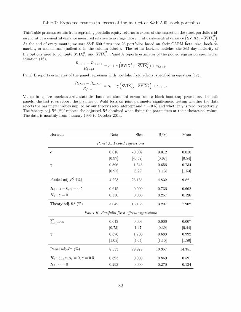
Table 7: Expected returns in excess of the market of S&P 500 stock portfolios

This Table presents results from regressing portfolio equity returns in excess of the market on the stock portfolio’s id-

iosyncratic risk-neutral variance measured relative to average idiosyncratic risk-neutral variance(

SVIX2i,t−SVIX

2

t

).

At the end of every month, we sort S&P 500 firms into 25 portfolios based on their CAPM beta, size, book-to-market, or momentum (indicated in the column labels). The return horizon matches the 365 day-maturity of

the options used to compute SVIX2i,t and SVIX

2

t . Panel A reports estimates of the pooled regression specified inequation (16),

Ri,t+1 −Rm,t+1

Rf,t+1= α+ γ

(SVIX2

i,t−SVIX2

t

)+ εi,t+1.

Panel B reports estimates of the panel regression with portfolio fixed effects, specified in equation (17),

Ri,t+1 −Rm,t+1

Rf,t+1= αi + γ

(SVIX2

i,t−SVIX2

t

)+ εi,t+1.

Values in square brackets are t-statistics based on standard errors from a block bootstrap procedure. In bothpanels, the last rows report the p-values of Wald tests on joint parameter significance, testing whether the datarejects the parameter values implied by our theory (zero intercept and γ = 0.5) and whether γ is zero, respectively.The ‘theory adj-R2 (%)’ reports the adjusted-R2 obtained when fixing the parameters at their theoretical values.The data is monthly from January 1996 to October 2014.



α 0.018 -0.009 0.012 0.010

[0.97] [-0.57] [0.67] [0.54]

γ 0.396 1.543 0.656 0.734

[0.97] [6.29] [1.13] [1.53]

Pooled adj-R2 (%) 4.223 26.165 4.832 9.821

H0 : α = 0, γ = 0.5 0.615 0.000 0.736 0.662

H0 : γ = 0 0.330 0.000 0.257 0.126

Theory adj-R2 (%) 3.042 13.138 3.207 7.902

Panel B. Portfolio fixed-effects regressions∑i wiαi 0.013 0.003 0.006 0.007

[0.73] [1.47] [0.39] [0.44]

γ 0.676 1.700 0.683 0.992

[1.05] [4.64] [1.10] [1.50]

Panel adj-R2 (%) 8.533 29.979 10.357 14.351

H0 :∑i wiαi = 0, γ = 0.5 0.693 0.000 0.869 0.591

H0 : γ = 0 0.293 0.000 0.270 0.134

32

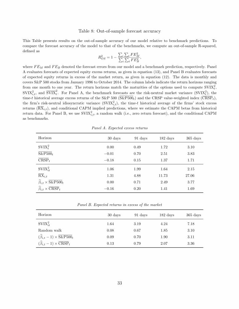
Table 8: Out-of-sample forecast accuracy

This Table presents results on the out-of-sample accuracy of our model relative to benchmark predictions. To

compare the forecast accuracy of the model to that of the benchmarks, we compute an out-of-sample R-squared,

defined as

R2OS = 1−

∑i

∑t FE

2M∑

i

∑t FE

2B

,

where FEM and FEB denoted the forecast errors from our model and a benchmark prediction, respectively. Panel

A evaluates forecasts of expected equity excess returns, as given in equation (13), and Panel B evaluates forecasts

of expected equity returns in excess of the market return, as given in equation (12). The data is monthly and

covers S&P 500 stocks from January 1996 to October 2014. The column labels indicate the return horizons ranging

from one month to one year. The return horizons match the maturities of the options used to compute SVIX2t ,

SVIX2i,t, and SVIX

2

t . For Panel A, the benchmark forecasts are the risk-neutral market variance (SVIX2t ), the

time-t historical average excess returns of the S&P 500 (S&P500t) and the CRSP value-weighted index (CRSPt),

the firm’s risk-neutral idiosyncratic variance (SVIX2i,t), the time-t historical average of the firms’ stock excess

returns (RXi,t), and conditional CAPM implied predictions, where we estimate the CAPM betas from historical

return data. For Panel B, we use SVIX2i,t, a random walk (i.e., zero return forecast), and the conditional CAPM

as benchmarks.

Panel A. Expected excess returns


SVIX2t 0.00 0.49 1.72 3.10

S&P500t −0.01 0.70 2.51 3.83

CRSPt −0.18 0.15 1.37 1.71

SVIX2it 1.06 1.99 1.64 2.15

RXi,t 1.31 4.88 11.73 27.06

βi,t × S&P500t 0.00 0.71 2.49 3.77

βi,t × CRSPt −0.16 0.20 1.41 1.69

Panel B. Expected returns in excess of the market


SVIX2it 1.64 3.19 4.24 7.18

Random walk 0.08 0.67 1.85 3.10

(βi,t − 1)× S&P500t 0.09 0.70 1.90 3.11

(βi,t − 1)× CRSPt 0.13 0.79 2.07 3.36

33

Table 9: Portfolio performance with monthly rebalancing

This Table summarizes the performance of monthly rebalanced portfolios invested in S&P 500 stocks from January1996 to October 2014. We compare the performance of a portfolio based on model-implied expected excess returnsto the market benchmark (a value-weighted portfolio) and a naive diversification strategy (an equally-weightedportfolio). For the model portfolio, we apply a rank weighting scheme,

wXSi,t =rank[EtRi,t+1]θ∑i rank[EtRi,t+1]θ

,

which assigns portfolio weights wXSi,t that increase in expected excess returns, does not allow for short positions,

and ensures that the investor is fully invested in the stock market, i.e.∑i w

XSi,t = 1. The parameter θ controls

the aggressiveness of the strategy, and we set θ = 1. For the model forecast-based portfolios, we report annualizedaverage excess returns along with their associated standard deviations and Sharpe ratios as well as their skewnessand excess kurtosis. For the benchmark portfolios we additionally report the performance fee (following Fleminget al., 2001) that a risk-averse investor with relative risk aversion ρ ∈ {1, 3, 10} would be willing to pay to switchfrom the benchmark strategy to the model portfolio. The column labels indicate the variance horizon used in themodel forecast.


Portfolio performance based on model forecasts

Mean (%p.a.) 10.48 11.03 11.06 11.45

Sd (%p.a.) 21.70 21.74 21.79 21.81

Sharpe ratio (p.a.) 0.48 0.51 0.51 0.52

Skewness −0.25 −0.21 −0.22 −0.21

Excess kurtosis 1.61 1.54 1.60 1.51

Comparison to value-weighted portfolio

Sharpe ratio (p.a.) 0.45 0.44 0.43 0.41

Skewness −0.62 −0.60 −0.59 −0.58


Performance fee with ρ = 1 (%p.a.) 3.02 3.61 3.81 4.44



Comparison to equally-weighted portfolio

Sharpe ratio (p.a.) 0.54 0.56 0.55 0.55

Skewness −0.48 −0.46 −0.46 −0.45





34

Table 10: Portfolio performance with daily rebalancing

This Table summarizes the performance of daily rebalanced portfolios invested in S&P 500 stocks from January1996 to October 2014. We compare the performance of a portfolio based on model-implied expected excess returnsto the market benchmark (a value-weighted portfolio) and a naive diversification strategy (an equally-weightedportfolio). For the model portfolio, we apply a rank weighting scheme,


,







Mean (%p.a.) 12.68 12.48 12.40 12.48

Sd (%p.a.) 24.89 24.94 24.93 24.83

Sharpe ratio (p.a.) 0.51 0.50 0.50 0.50

Skewness −0.11 −0.11 −0.12 −0.12



Sharpe ratio (p.a.) 0.38 0.38 0.38 0.38

Skewness −0.18 −0.18 −0.18 −0.18






Sharpe ratio (p.a.) 0.51 0.51 0.51 0.52

Skewness −0.21 −0.21 −0.21 −0.21





35

Table 11: Performance of aggressive portfolios with daily rebalancing

This Table summarizes the performance of daily rebalanced portfolios invested in S&P 500 stocks from January1996 to October 2014. We compare the performance of a portfolio based on model-implied expected excess returnsto the market benchmark (a value-weighted portfolio) and a naive diversification strategy (an equally-weightedportfolio). For the model portfolio, we apply a rank weighting scheme,


,





30 days 91 days 182 days 365 days


Mean (%p.a.) 13.86 13.49 13.38 13.49

Sd (%p.a.) 27.70 27.78 27.76 27.59

Sharpe ratio (p.a.) 0.50 0.49 0.48 0.49

Skewness −0.03 −0.04 −0.04 −0.04



Sharpe ratio (p.a.) 0.38 0.38 0.38 0.38

Skewness −0.18 −0.18 −0.18 −0.18






Sharpe ratio (p.a.) 0.51 0.51 0.51 0.52

Skewness −0.21 −0.21 −0.21 −0.21





36

Table 12: Performance of size- and value-portfolios with monthly rebalancing

This Table summarizes the performance of monthly rebalanced portfolios invested in a subset of S&P 500 stocks,conditional on firm size or book-to-market. At every portfolio rebalancing date t, we classify firms as small (big)when their market capitalization is in the bottom (top) tertile of the time-t distribution across all firms in oursample. Similarly, we classify firms as value (growth) stocks when their book-to-market ratio is within the top(bottom) tertile of the book-to-market distribution at time t. The sample period is from January 1996 to October2014. We compare the performance of a portfolio based on model-implied expected excess returns to a value-weighted portfolio and a naive diversification strategy (an equally-weighted portfolio). For the model portfolio, weapply a rank weighting scheme,


,





Small Big Value Growth


Mean (%p.a.) 17.06 6.85 14.59 9.05

Sd (%p.a.) 27.06 19.48 22.99 23.32

Sharpe ratio (p.a.) 0.63 0.35 0.63 0.39

Skewness 0.31 −0.66 −0.20 −0.23



Sharpe ratio (p.a.) 0.55 0.37 0.44 0.38

Skewness −0.24 −0.56 −0.73 −0.46






Sharpe ratio (p.a.) 0.63 0.40 0.61 0.44

Skewness −0.02 −0.69 −0.49 −0.43




Performance fee with ρ = 10 (%p.a.) 2.17 −0.03 2.21 0.16

37

Table 13: Performance of aggressive size- and value-portfolios with daily rebalancing

This Table summarizes the performance of daily rebalanced portfolios invested in a subset of S&P 500 stocks,conditional on firm size or book-to-market. At every portfolio rebalancing date t, we classify firms as small (big)when their market capitalization is in the bottom (top) tertile of the time-t distribution across all firms in oursample. Similarly, we classify firms as value (growth) stocks when their book-to-market ratio is within the top(bottom) tertile of the book-to-market distribution at time t. The sample period is from January 1996 to October2014. We compare the performance of a portfolio based on model-implied expected excess returns to a value-weighted portfolio and a naive diversification strategy (an equally-weighted portfolio). For the model portfolio, weapply a rank weighting scheme,


,





Small Big Value Growth


Mean (%p.a.) 21.84 9.90 19.92 12.31

Sd (%p.a.) 30.88 26.67 29.52 29.37

Sharpe ratio (p.a.) 0.71 0.37 0.67 0.42

Skewness 0.09 0.06 0.05 0.26



Sharpe ratio (p.a.) 0.53 0.31 0.38 0.32

Skewness −0.13 −0.12 −0.18 −0.04






Sharpe ratio (p.a.) 0.63 0.37 0.57 0.42

Skewness −0.07 −0.16 −0.19 −0.02





38

Figure 2: Option-implied equity variance of S&P 100 firms

This Figure plots the time-series of the risk-neutral variance of the market (SVIX2t ) and of stocks’ average idiosyn-

cratic risk-neutral variance (SVIX2

t ). We compute SVIX2t from equity index options on the S&P 100. SVIX

2

t is thevalue-weighted sum of S&P 100 stocks’ idiosyncratic risk-neutral variance computed from individual firm equityoptions. Panels A through D present the variance series implied by equity options with maturities of one, three,six, and twelve months, respectively. The data is daily from January 1996 to October 2014.

Panel A. One-month horizon

Sto

ck v

aria

nce

0.0

0.2

0.4

0.6

Jan/96 Jan/99 Jan/02 Jan/05 Jan/08 Jan/11 Jan/14

SVIXt2

SVIXt2

Panel C. Six-month horizon

Sto

ck v

aria

nce

0.0

0.1

0.2

0.3

0.4


SVIXt2

SVIXt2

Panel B. Three-month horizon

Sto

ck v

aria

nce

0.0

0.1

0.2

0.3

0.4

0.5


SVIXt2

SVIXt2

Panel D. One-year horizon

Sto

ck v

aria

nce

0.00

0.10

0.20

0.30


SVIXt2

SVIXt2

39

Figure 3: Option-implied equity variance of S&P 500 firms

This Figure plots the time-series of the risk-neutral variance of the market (SVIX2t ) and of stocks’ average idiosyn-

cratic risk-neutral variance (SVIX2

t ). We compute SVIX2t from equity index options on the S&P 500. SVIX

2

t is thevalue-weighted sum of S&P 500 stocks’ idiosyncratic risk-neutral variance computed from individual firm equityoptions. Panels A through D present the variance series implied by equity options with maturities of one, three,six, and twelve months, respectively. The data is daily from January 1996 to October 2014.


Sto

ck v

aria

nce

0.0

0.2

0.4

0.6


SVIXt2

SVIXt2

Panel C. Six-month horizon

Sto

ck v

aria

nce

0.0

0.1

0.2

0.3

0.4


SVIXt2

SVIXt2

Panel B. Three-month horizon

Sto

ck v

aria

nce

0.0

0.1

0.2

0.3

0.4

0.5


SVIXt2

SVIXt2

Panel D. One-year horizon

Sto

ck v

aria

nce

0.00

0.10

0.20

0.30


SVIXt2

SVIXt2

40

Figure 4: Beta, size, value, momentum, and option-implied equity variance

This Figure reports averages of idiosyncratic risk-neutral variance (SVIX2i,t, computed from individual firm equity

options) of S&P 500 stocks, conditional on firm beta, size, book-to-market, and momentum. At every date t, weassign stocks to decile portfolios based on on their characteristics and report the time-series averages of SVIX2

i,t

across deciles using SVIX2i,t-horizons of one year (Panels A to D). The sample period is January 1996 to October

2014.

Panel A. Beta

High P.2 P.3 P.4 P.5 P.6 P.7 P.8 P.9 Low

0.00

0.05

0.10

0.15

0.20

0.25

0.30

Panel B. Size

Small P.2 P.3 P.4 P.5 P.6 P.7 P.8 P.9 Big

0.00

0.05

0.10

0.15

0.20

0.25

Panel C. Book-to-market

Value P.2 P.3 P.4 P.5 P.6 P.7 P.8 P.9 Growth

0.00

0.05

0.10

0.15

0.20

0.25

Panel D. Momentum

Winner P.2 P.3 P.4 P.5 P.6 P.7 P.8 P.9 Loser

0.00

0.05

0.10

0.15

0.20

0.25

41

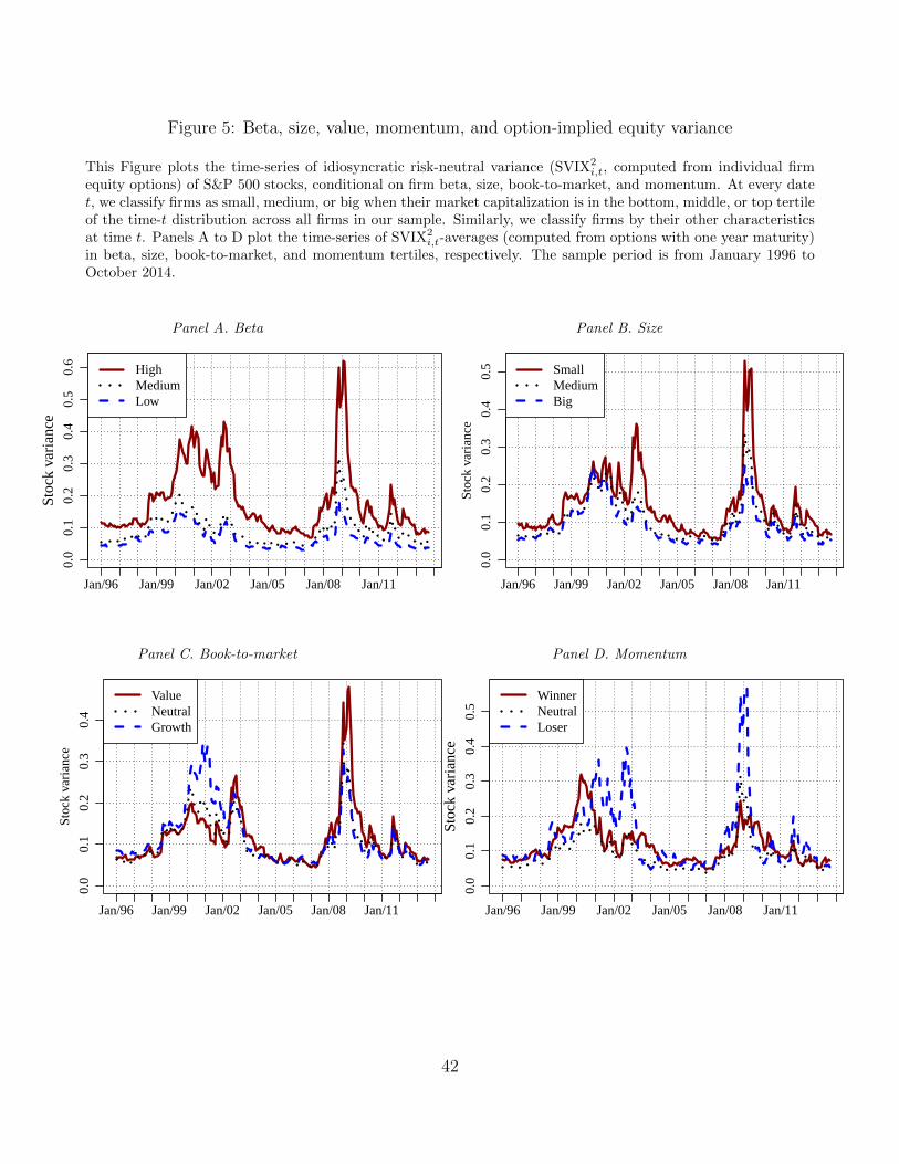
Figure 5: Beta, size, value, momentum, and option-implied equity variance

This Figure plots the time-series of idiosyncratic risk-neutral variance (SVIX2i,t, computed from individual firm

equity options) of S&P 500 stocks, conditional on firm beta, size, book-to-market, and momentum. At every datet, we classify firms as small, medium, or big when their market capitalization is in the bottom, middle, or top tertileof the time-t distribution across all firms in our sample. Similarly, we classify firms by their other characteristicsat time t. Panels A to D plot the time-series of SVIX2

i,t-averages (computed from options with one year maturity)in beta, size, book-to-market, and momentum tertiles, respectively. The sample period is from January 1996 toOctober 2014.

Panel A. Beta

Sto

ck v

aria

nce

0.0

0.1

0.2

0.3

0.4

0.5

0.6

Jan/96 Jan/99 Jan/02 Jan/05 Jan/08 Jan/11

HighMediumLow


Sto

ck v

aria

nce

0.0

0.1

0.2

0.3

0.4


ValueNeutralGrowth

Panel B. Size

Sto

ck v

aria

nce

0.0

0.1

0.2

0.3

0.4

0.5


SmallMediumBig

Panel D. Momentum

Sto

ck v

aria

nce

0.0

0.1

0.2

0.3

0.4

0.5


WinnerNeutralLoser

42

Figure 6: Average equity excess returns

This Figure presents results on the relation between a firm’s equity excess returns and its stock’s idiosyncraticrisk-neutral variance measured relative to average idiosyncratic risk-neutral variance. For the firm’s that havebeen constituents of the S&P 500 index throughout our sample period from January 1996 to October 2014, wecompute time-series averages of their excess returns and their idiosyncratic volatility relative to aggregate idiosyn-

cratic volatility(

SVIX2i −SVIX

2)

. We multiply the idiosyncratic variance estimate by 0.5 and plot the pairwise

combinations (blue crosses) for horizons of one, three, six, and, twelve months (Panels A to D). The black linerepresents the regression fit to the individual firm observations with slope coefficient and R-squared reported in theplot legend. Our theory implies that the slope coefficient of this regression should be one and that the interceptcorresponds to the average excess return of the market. The red diamonds represent decile portfolios of firms

generated from ranking firms by their average time-t decile classification based on(

SVIX2i,t−SVIX

2

t

)among all

S&P 500 firms over our sample period. Similarly, the triangles in orange represent portfolios of stocks formedaccording to their firms’ average size and book-to-market classification.

Panel A. One-month excess returns

−0.002 0.000 0.002 0.004 0.006 0.008

0.00

00.

010

0.02

0

0.5 × (SVIXi2 − SVIX2)

Exc

ess

retu

rn

Slope: 0.66, R−squ: 11%(SVIXi

2 − SVIX2) deciles3x3 Size x B/M

Panel C. Six-month excess returns

−0.01 0.00 0.01 0.02 0.03 0.04 0.05

0.00

0.05

0.10

0.15


Exc

ess

retu

rn

Slope: 1.03, R−squ: 19.6%(SVIXi


Panel B. Three-month excess returns

−0.005 0.005 0.015 0.025

0.00

0.02

0.04

0.06

0.08


Exc

ess

retu

rn

Slope: 0.85, R−squ: 16%(SVIXi


Panel D. One-year excess returns

−0.02 0.00 0.02 0.04 0.06 0.08 0.10

0.0

0.1

0.2

0.3

0.4


Exc

ess

retu

rn

Slope: 1.12, R−squ: 18.5%(SVIXi


43

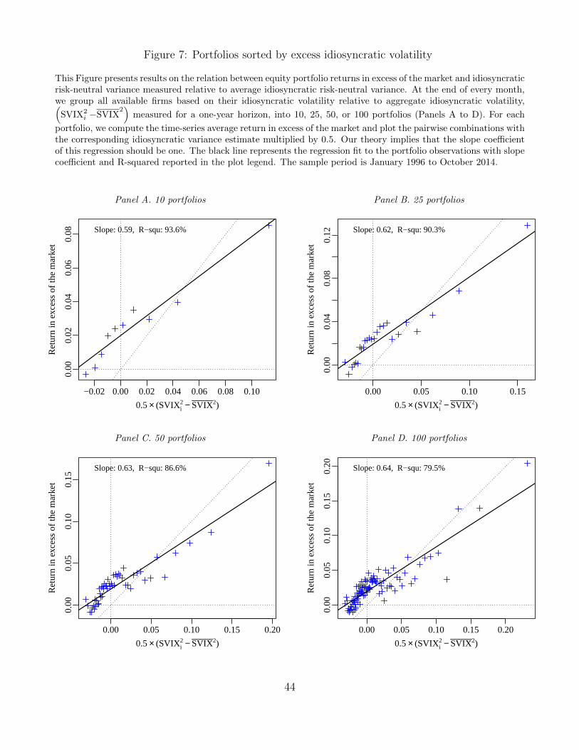
Figure 7: Portfolios sorted by excess idiosyncratic volatility

This Figure presents results on the relation between equity portfolio returns in excess of the market and idiosyncraticrisk-neutral variance measured relative to average idiosyncratic risk-neutral variance. At the end of every month,we group all available firms based on their idiosyncratic volatility relative to aggregate idiosyncratic volatility,(

SVIX2i −SVIX

2)

measured for a one-year horizon, into 10, 25, 50, or 100 portfolios (Panels A to D). For each

portfolio, we compute the time-series average return in excess of the market and plot the pairwise combinations withthe corresponding idiosyncratic variance estimate multiplied by 0.5. Our theory implies that the slope coefficientof this regression should be one. The black line represents the regression fit to the portfolio observations with slopecoefficient and R-squared reported in the plot legend. The sample period is January 1996 to October 2014.

Panel A. 10 portfolios

−0.02 0.00 0.02 0.04 0.06 0.08 0.10

0.00

0.02

0.04

0.06

0.08


Ret

urn

in e

xces

s of

the

mar

ket Slope: 0.59, R−squ: 93.6%

Panel C. 50 portfolios

0.00 0.05 0.10 0.15 0.20

0.00

0.05

0.10

0.15


Ret

urn

in e

xces

s of

the

mar


Panel B. 25 portfolios

0.00 0.05 0.10 0.15

0.00

0.04

0.08

0.12


Ret

urn

in e

xces

s of

the

mar


Panel D. 100 portfolios

0.00 0.05 0.10 0.15 0.20

0.00

0.05

0.10

0.15

0.20


Ret

urn

in e

xces

s of

the

mar


44

Figure 8: Portfolios sorted by beta, size, book-to-market, and momentum

This Figure presents results on the relation between equity portfolio returns in excess of the market and idiosyncraticrisk-neutral variance measured relative to average idiosyncratic risk-neutral variance. At the end of every month,we form 25 portfolios based on firms’ beta, size, book-to-market, or mometum (Panels A to D). For each portfolio,we compute the time-series average return in excess of the market and plot the pairwise combinations with thecorresponding idiosyncratic variance estimate multiplied by 0.5. The black line represents the regression fit to theportfolio observations with slope coefficient and R-squared reported in the plot legend. Our theory implies thatthe slope coefficient of this regression should be one. The sample period is January 1996 to October 2014.

Panel A. 25 Beta portfolios

−0.02 0.00 0.02 0.04 0.06 0.08 0.10 0.12−0.

010.

010.

020.

030.

040.

05


Ret

urn

in e

xces

s of

the

mar


Panel C. 25 B/M portfolios

0.00 0.01 0.02 0.03 0.04

0.00

0.02

0.04

0.06


Ret

urn

in e

xces

s of

the

mar

ket Slope: 0.9, R−squ: 11%

Panel B. 25 Size portfolios

0.00 0.01 0.02 0.03 0.04 0.05

0.00

0.05

0.10

0.15


Ret

urn

in e

xces

s of

the

mar


Panel D. 25 Momentum portfolios

0.00 0.02 0.04 0.06 0.08

0.00

0.02

0.04

0.06


Ret

urn

in e

xces

s of

the

mar


45

Figure 9: Individual firm expected equity excess returns

This Figure plots the time-series of real-time expected excess returns for selected individualfirms. According to the SIC-based industry definitions provided on Kenneth French’s website(http://mba.tuck.dartmouth.edu/pages/faculty/ken.french/), IBM, Microsoft, and Apple belong to the in-dustry ‘Business Equipment – Computers, Software, and Electronic Equipment.’ Citigroup, JP Morgan, and Bankof America fall into the industry ‘Banking, Insurance, Real Estate, Trading.’ The forecast horizon is one year andthe sample period is January 1996 to October 2014.

IBM

Exp

ecte

d E

xces

s R

etur

n

0.00

0.02

0.04

0.06

0.08


Microsoft

Exp

ecte

d E

xces

s R

etur

n

0.00

0.02

0.04

0.06

0.08

0.10


Apple

Exp

ecte

d E

xces

s R

etur

n

0.05

0.10

0.15

0.20


Citigroup

Exp

ecte

d E

xces

s R

etur

n

0.0

0.2

0.4

0.6

0.8

1.0


JP Morgan

Exp

ecte

d E

xces

s R

etur

n

0.00

0.05

0.10

0.15

0.20


Bank of America

Exp

ecte

d E

xces

s R

etur

n

0.0

0.2

0.4

0.6

0.8


46

Figure 10: Individual firms expected excess returns and expected excess market returns

This Figure plots the time-series of real-time expected excess returns and real-time expected returns in excessof the market for selected individual firms. According to the SIC-based industry definitions provided on Ken-neth French’s website (http://mba.tuck.dartmouth.edu/pages/faculty/ken.french/), Apple belongs to the industry‘Business Equipment – Computers, Software, and Electronic Equipment.’ and JP Morgan falls into the industry‘Banking, Insurance, Real Estate, Trading.’ The forecast horizon is one year and the sample period is January1996 to October 2014.


APPLE INC

Exp

ecte

d E

xces

s R

etur

n

0.00

0.05

0.10

0.15

0.20


JPMORGAN CHASE & CO

Exp

ecte

d E

xces

s R

etur

n

0.00

0.05

0.10

0.15

0.20



APPLE INC

Exp

ecte

d R

etur

n in

Exc

ess

of th

e M

arke

t

0.00

0.05

0.10

0.15

0.20


JPMORGAN CHASE & CO

Exp

ecte

d R

etur

n in

Exc

ess

of th

e M

arke

t

0.00

0.05

0.10


47

Figure 11: Cumulative portfolio returns

This Figure plots the cumulative returns of daily rebalanced portfolios invested in S&P 500 stocks from January1996 to October 2014. We compare the performance of a portfolio based on model-implied expected returns to themarket benchmark (a value-weighted portfolio) and a naive diversification strategy (an equally-weighted portfolio).For the model portfolio, we apply a rank weighting scheme,


,



XSi,t = 1. The parameter θ controls the

aggressiveness of the strategy. Panels A and B plot the cumulative portfolio returns when using forecasts based onone-month and one-year variance horizons, respectively, when setting θ = 1. Panels C and D plot the cumulativeportfolio returns for a more aggressive strategy that uses θ = 2.


Cum

ulat

ive

retu

rns

(log

scal

e)

12

510


ModelVWEWcash

Panel C. One-month horizon, aggressive

Cum

ulat

ive

retu

rns

(log

scal

e)

12

510


ModelVWEWcash

Panel B. One-year horizon

Cum

ulat

ive

retu

rns

(log

scal

e)

12

510


ModelVWEWcash

Panel D. One-year horizon, aggressive

Cum

ulat

ive

retu

rns

(log

scal

e)

12

510


ModelVWEWcash

48

Figure 12: Cumulative returns of size and value firm portfolios

This Figure plots the cumulative returns of daily rebalanced portfolios invested in S&P 500 stocks, conditional onfirm size or book-to-market. At every portfolio rebalancing date t, we classify firms as small (big) when their marketcapitalization is in the bottom (top) tertile of the time-t distribution across all firms in our sample. Similarly, weclassify firms as value (growth) stocks when their book-to-market ratio is within the top (bottom) tertile of thebook-to-market distribution at time t. The sample period is from January 1996 to October 2014. We comparethe performance of a portfolio based on model-implied expected returns to a value-weighted portfolio and a naivediversification strategy (an equally-weighted portfolio). For the model portfolio, we apply a rank weighting scheme,


,




aggressiveness of the strategy, and we set θ = 2. Panels A and B plot the cumulative returns for small and big firmportfolios, Panels C and D plot the cumulative returns from investing in value and growth stocks.

Panel A. Small firms

Cum

ulat

ive

retu

rns

(log

scal

e)

12

510

20

Feb/96 Feb/99 Feb/02 Feb/05 Feb/08 Feb/11

ModelVWEWcash

Panel C. Value firms

Cum

ulat

ive

retu

rns

(log

scal

e)

12

510

20


ModelVWEWcash

Panel B. Big firms

Cum

ulat

ive

retu

rns

(log

scal

e)

12

34

5


ModelVWEWcash

Panel D. Growth firms

Cum

ulat

ive

retu

rns

(log

scal

e)

12

34

56


ModelVWEWcash

49

Internet Appendix for

What is the Expected Return on a Stock?

(not for publication)

Internet Appendix – 1

IA.A Supplementary Material

This section shows (as promised in footnote 2) that the assumption that Ri,t+1Rg,t+1

is a tradable payoff is innocuous. Let E∗t be a risk-neutral measure; there may be

more than one, if markets are incomplete. Since Ri,t+1Rg,t+1 = 12R2i,t+1 + 1

2R2g,t+1 −

12

(Ri,t+1 −Rg,t+1)2,

1

R2f,t+1

E∗t Ri,t+1Rg,t+1 =1

2R2f,t+1

[E∗t R2

i,t+1 + E∗t R2g,t+1

]− 1

2var∗t

Ri,t+1 −Rg,t+1

Rf,t+1

.

We assume that the final term equals αi + λt. Without further loss of generality,

we may assume that∑

iwi,tαi = 0, so the above equation can be rewritten as

1

R2f,t+1

E∗t Ri,t+1Rg,t+1 − 1 =1

2R2f,t+1

[var∗t Ri,t+1 + var∗t Rg,t+1] + αi + λt. (IA.A.1)

Multiplying (IA.A.1) by wi,t and summing over i, it follows that

1

R2f,t+1

E∗t Rm,t+1Rg,t+1− 1 =1

2R2f,t+1

[∑i

wi,t var∗t Ri,t+1 + var∗t Rg,t+1

]+λt. (IA.A.2)

Subtracting (IA.A.2) from (IA.A.1), we find that

1

R2f,t+1

E∗t [(Ri,t+1 −Rm,t+1)Rg,t+1] =1

2

[var∗t

Ri,t+1

Rf,t+1

−∑i

wi,t var∗tRi,t+1

Rf,t+1

]+ αi.

The terms inside the square brackets on the right-hand side are uniquely determined

by option prices. So the left-hand side is too (since αi is a constant).

If we set Et(X) = Rf,t+1 Et XRg,t+1

, then Et is a risk-neutral measure. Hence

1

R2f,t+1

Et [(Ri,t+1 −Rm,t+1)Rg,t+1] =1

2

[var∗t

Ri,t+1

Rf,t+1

−∑i

wi,t var∗tRi,t+1

Rf,t+1

]+ αi.

But then by the definition of E, we have our result,

EtRi,t+1 −Rm,t+1

Rf,t+1

=1

2

[var∗t

Ri,t+1

Rf,t+1

−∑i

wi,t var∗tRi,t+1

Rf,t+1

]+ αi.


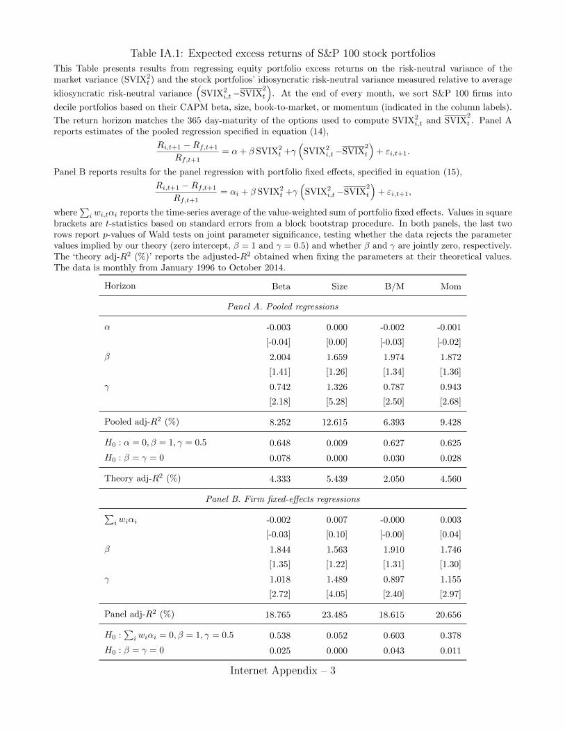
Table IA.1: Expected excess returns of S&P 100 stock portfolios

This Table presents results from regressing equity portfolio excess returns on the risk-neutral variance of themarket variance (SVIX2

t ) and the stock portfolios’ idiosyncratic risk-neutral variance measured relative to average


SVIX2i,t−SVIX

2

t

). At the end of every month, we sort S&P 100 firms into

decile portfolios based on their CAPM beta, size, book-to-market, or momentum (indicated in the column labels).

The return horizon matches the 365 day-maturity of the options used to compute SVIX2i,t and SVIX

2

t . Panel Areports estimates of the pooled regression specified in equation (14),

Ri,t+1 −Rf,t+1


t +γ(

SVIX2i,t−SVIX

2

t

)+ εi,t+1.

Panel B reports results for the panel regression with portfolio fixed effects, specified in equation (15),

Ri,t+1 −Rf,t+1


t +γ(

SVIX2i,t−SVIX

2

t

)+ εi,t+1,

where∑i wi,tαi reports the time-series average of the value-weighted sum of portfolio fixed effects. Values in square

brackets are t-statistics based on standard errors from a block bootstrap procedure. In both panels, the last tworows report p-values of Wald tests on joint parameter significance, testing whether the data rejects the parametervalues implied by our theory (zero intercept, β = 1 and γ = 0.5) and whether β and γ are jointly zero, respectively.The ‘theory adj-R2 (%)’ reports the adjusted-R2 obtained when fixing the parameters at their theoretical values.The data is monthly from January 1996 to October 2014.



α -0.003 0.000 -0.002 -0.001

[-0.04] [0.00] [-0.03] [-0.02]

β 2.004 1.659 1.974 1.872

[1.41] [1.26] [1.34] [1.36]

γ 0.742 1.326 0.787 0.943

[2.18] [5.28] [2.50] [2.68]

Pooled adj-R2 (%) 8.252 12.615 6.393 9.428

H0 : α = 0, β = 1, γ = 0.5 0.648 0.009 0.627 0.625

H0 : β = γ = 0 0.078 0.000 0.030 0.028

Theory adj-R2 (%) 4.333 5.439 2.050 4.560

Panel B. Firm fixed-effects regressions∑i wiαi -0.002 0.007 -0.000 0.003

[-0.03] [0.10] [-0.00] [0.04]

β 1.844 1.563 1.910 1.746

[1.35] [1.22] [1.31] [1.30]

γ 1.018 1.489 0.897 1.155

[2.72] [4.05] [2.40] [2.97]

Panel adj-R2 (%) 18.765 23.485 18.615 20.656

H0 :∑i wiαi = 0, β = 1, γ = 0.5 0.538 0.052 0.603 0.378

H0 : β = γ = 0 0.025 0.000 0.043 0.011


Table IA.2: Expected excess returns of S&P 500 stock portfolios

This Table presents results from regressing equity portfolio excess returns on the risk-neutral variance of themarket variance (SVIX2

t ) and the stock portfolios’ idiosyncratic risk-neutral variance measured relative to average


SVIX2i,t−SVIX

2

t

). At the end of every month, we sort S&P 500 firms into

decile portfolios based on their CAPM beta, size, book-to-market, or momentum (indicated in the column labels).

The return horizon matches the 365 day-maturity of the options used to compute SVIX2i,t and SVIX

2

t . Panel Areports estimates of the pooled regression specified in equation (14),

Ri,t+1 −Rf,t+1


t +γ(

SVIX2i,t−SVIX

2

t

)+ εi,t+1.

Panel B reports results for the panel regression with portfolio fixed effects, specified in equation (15),

Ri,t+1 −Rf,t+1


t +γ(

SVIX2i,t−SVIX

2

t

)+ εi,t+1,

where∑i wi,tαi reports the time-series average of the value-weighted sum of portfolio fixed effects. Values in square

brackets are t-statistics based on standard errors from a block bootstrap procedure. In both panels, the last tworows report p-values of Wald tests on joint parameter significance, testing whether the data rejects the parametervalues implied by our theory (zero intercept, β = 1 and γ = 0.5) and whether β and γ are jointly zero, respectively.The ‘theory adj-R2 (%)’ reports the adjusted-R2 obtained when fixing the parameters at their theoretical values.The data is monthly from January 1996 to October 2014.



α -0.020 -0.018 -0.021 -0.021

[-0.29] [-0.26] [-0.30] [-0.29]

β 3.078 2.271 3.064 2.875

[1.86] [1.57] [1.81] [1.77]

γ 0.326 1.414 0.399 0.635

[0.90] [3.52] [0.95] [1.42]

Pooled adj-R2 (%) 7.499 15.306 8.120 9.621

H0 : α = 0, β = 1, γ = 0.5 0.065 0.143 0.081 0.271

H0 : β = γ = 0 0.166 0.002 0.183 0.155

Theory adj-R2 (%) 1.108 5.193 0.857 3.314

Panel B. Portfolio fixed-effects regressions∑i wiαi -0.018 -0.006 -0.027 -0.017

[-0.27] [-0.08] [-0.38] [-0.24]

β 2.924 2.181 3.070 2.704

[1.83] [1.52] [1.82] [1.71]

γ 0.527 1.530 0.392 0.855

[1.03] [2.48] [0.91] [1.44]

Panel adj-R2 (%) 19.920 27.481 22.470 22.001

H0 :∑i wiαi = 0, β = 1, γ = 0.5 0.110 0.359 0.105 0.390

H0 : β = γ = 0 0.186 0.030 0.182 0.173


Table IA.3: Performance of aggressive size/value-portfolios with daily rebalancing

This Table summarizes the performance of daily rebalanced portfolios invested in a subset of S&P 500 stocks,conditional on firm size and book-to-market. At every portfolio rebalancing date t, we classify firms as small(big) when their market capitalization is in the bottom (top) tertile of the time-t distribution across all firms inour sample. Similarly, we classify firms as value (growth) stocks when their book-to-market ratio is within thetop (bottom) tertile of the book-to-market distribution at time t. We report results for firms that are classifiedas small value, small growth, big value, and big growth. The sample period is from January 1996 to October2014. We compare the performance of a portfolio based on model-implied expected excess returns (based on avariance horizon of one year) to a value-weighted portfolio and a naive diversification strategy (an equally-weightedportfolio). For the model portfolio, we apply a rank weighting scheme,


,




the aggressiveness of the strategy, and we set θ = 2. For the model forecast-based portfolios, we report annualizedaverage excess returns along with their associated standard deviations and Sharpe ratios as well as their skewnessand excess kurtosis. For the benchmark portfolios we additionally report the performance fee (following Fleminget al., 2001) that a risk-averse investor with relative risk aversion ρ ∈ {1, 3, 10} would be willing to pay to switchfrom the benchmark strategy to the model portfolio.

Small Value Small Growth Big Value Big Growth


Mean (%p.a.) 25.52 21.24 11.71 10.06

Sd (%p.a.) 32.52 35.49 30.41 26.81

Sharpe ratio (p.a.) 0.78 0.60 0.39 0.38

Skewness 0.11 0.52 0.12 0.21

Excess kurtosis 7.21 6.94 12.31 5.62


Sharpe ratio (p.a.) 0.55 0.42 0.29 0.32

Skewness −0.22 0.25 −0.11 −0.02






Sharpe ratio (p.a.) 0.67 0.52 0.36 0.37

Skewness −0.11 0.27 −0.23 −0.05






Figure IA.1: Beta, size, value, momentum, and option-implied equity variance

This Figure reports averages of idiosyncratic risk-neutral variance (SVIX2i,t, computed from individual firm equity

options) of S&P 500 stocks, conditional on firm beta, size, book-to-market, and momentum. At every date t, weassign stocks to decile portfolios based on on their characteristics and report the time-series averages of SVIX2

i,t

across deciles using horizons of one month (Panels A to D). The sample period is January 1996 to October 2014.

Panel A. Beta

High P.2 P.3 P.4 P.5 P.6 P.7 P.8 P.9 Low

0.00

0.05

0.10

0.15

0.20

0.25

0.30

Panel B. Size

Small P.2 P.3 P.4 P.5 P.6 P.7 P.8 P.9 Big

0.00

0.05

0.10

0.15

0.20

0.25


Value P.2 P.3 P.4 P.5 P.6 P.7 P.8 P.9 Growth

0.00

0.05

0.10

0.15

0.20

0.25

Panel D. Momentum

Winner P.2 P.3 P.4 P.5 P.6 P.7 P.8 P.9 Loser

0.00

0.05

0.10

0.15

0.20

0.25


Figure IA.2: Beta, size, value, momentum, and option-implied equity variance


equity options) of S&P 500 stocks, conditional on firm beta, size, book-to-market, and momentum. At every datet, we classify firms as small, medium, or big when their market capitalization is in the bottom, middle, or top tertileof the time-t distribution across all firms in our sample. Similarly, we classify firms by their other characteristics attime t. Panels A to D plot the time-series of SVIX2

i,t-averages (computed from options with one month maturity)in beta, size, book-to-market, and momentum tertiles, respectively. The sample period is from January 1996 toOctober 2014.

Panel A. Beta

Sto

ck v

aria

nce

0.0

0.2

0.4

0.6

0.8


HighMediumLow


Sto

ck v

aria

nce

0.0

0.2

0.4

0.6


ValueNeutralGrowth

Panel B. Size

Sto

ck v

aria

nce

0.0

0.2

0.4

0.6

0.8


SmallMediumBig

Panel D. Momentum

Sto

ck v

aria

nce

0.0

0.2

0.4

0.6

0.8


WinnerNeutralLoser


Figure IA.3: Size, value, and option-implied equity variance


equity options) of S&P 500 stocks, conditional on firm size and book-to-market. At every date t, we classify firmsas small, medium, or big when their market capitalization is in the bottom, middle, or top tertile of the time-tdistribution across all firms in our sample. Similarly, we classify firms as value, neutral, or growth stocks whentheir book-to-market ratio is within the top, middle, or bottom tertile of the book-to-market distribution at timet. Panels A and B plot the time-series of SVIX2

i,t-averages for intersections of size and value tertiles. The sampleperiod is from January 1996 to October 2014.

Panel A. Small stocks

Sto

ck v

aria

nce

0.0

0.1

0.2

0.3

0.4

0.5

0.6


Small ValueSmall Growth

Panel B. Big stocks

Sto

ck v

aria

nce

0.0

0.1

0.2

0.3

0.4

0.5

0.6


Big ValueBig Growth


Figure IA.4: Portfolios sorted by size and book-to-market

This Figure presents results on the relation between equity portfolio returns in excess of the market and idiosyncraticrisk-neutral variance measured relative to average idiosyncratic risk-neutral variance. At the end of every month,we form 25 portfolios based on a 5x5 double sort on size and book-to-market. For each portfolio, we computethe time-series average return in excess of the market and plot the pairwise combinations with the correspondingidiosyncratic variance estimate multiplied by 0.5. The black line represents the regression fit to the portfolioobservations with slope coefficient and R-squared reported in the plot legend. Our theory implies that the slopecoefficient of this regression should be one and that the intercept corresponds to the average excess return of themarket. The sample period is January 1996 to October 2014.

25 Size x B/M portfolios

0.00 0.01 0.02 0.03 0.04

0.00

0.02

0.04

0.06

0.08

0.10


Ret

urn

in e

xces

s of

the

mar



Figure IA.5: Cumulative returns of size and value firm portfolios

This Figure plots the cumulative returns of daily rebalanced portfolios invested in S&P 500 stocks, conditionalon firm size and book-to-market. At every portfolio rebalancing date t, we classify firms as small (big) whentheir market capitalization is in the bottom (top) tertile of the time-t distribution across all firms in our sample.Similarly, we classify firms as value (growth) stocks when their book-to-market ratio is within the top (bottom)tertile of the book-to-market distribution at time t. The sample period is from January 1996 to October 2014. Wecompare the performance of a portfolio based on model-implied expected returns to a value-weighted portfolio anda naive diversification strategy (an equally-weighted portfolio). For the model portfolio, we apply a rank weightingscheme,


,




aggressiveness of the strategy, and we set θ = 2. Panels A to D plot the cumulative returns of portfolios containingsmall value stocks, small growth stocks, big value stocks, and big growth stocks.

Panel A. Small value firms

Cum

ulat

ive

retu

rns

(log

scal

e)

12

510

2050


ModelVWEWcash

Panel C. Big value firms

Cum

ulat

ive

retu

rns

(log

scal

e)

12

34

56


ModelVWEWcash

Panel B. Small growth firms

Cum

ulat

ive

retu

rns

(log

scal

e)

12

510

20


ModelVWEWcash

Panel D. Big growth firms

Cum

ulat

ive

retu

rns

(log

scal

e)

12

34

5


ModelVWEWcash


Figure IA.6: Expected returns for Ford and General Motors

This Figure plots the time-series of real-time expected excess returns and real-time expected returns in excess ofthe market for Ford and General Motors. According to the SIC-based industry definitions provided on KennethFrench’s website (http://mba.tuck.dartmouth.edu/pages/faculty/ken.french/), both firms belong to the industry‘Consumer Durables.’ The forecast horizon is one year and the sample period is January 1996 to October 2014.


FORD MOTOR CO

Exp

ecte

d E

xces

s R

etur

n

0.0

0.2

0.4

0.6

0.8


GENERAL MOTORS CO

Exp

ecte

d E

xces

s R

etur

n

0.00

0.05

0.10

0.15

0.20



FORD MOTOR CO

Exp

ecte

d R

etur

n in

Exc

ess

of th

e M

arke

t

0.0

0.2

0.4

0.6

0.8


GENERAL MOTORS CO

Exp

ecte

d R

etur

n in

Exc

ess

of th

e M

arke

t

−0.

050.

000.

050.

100.

15



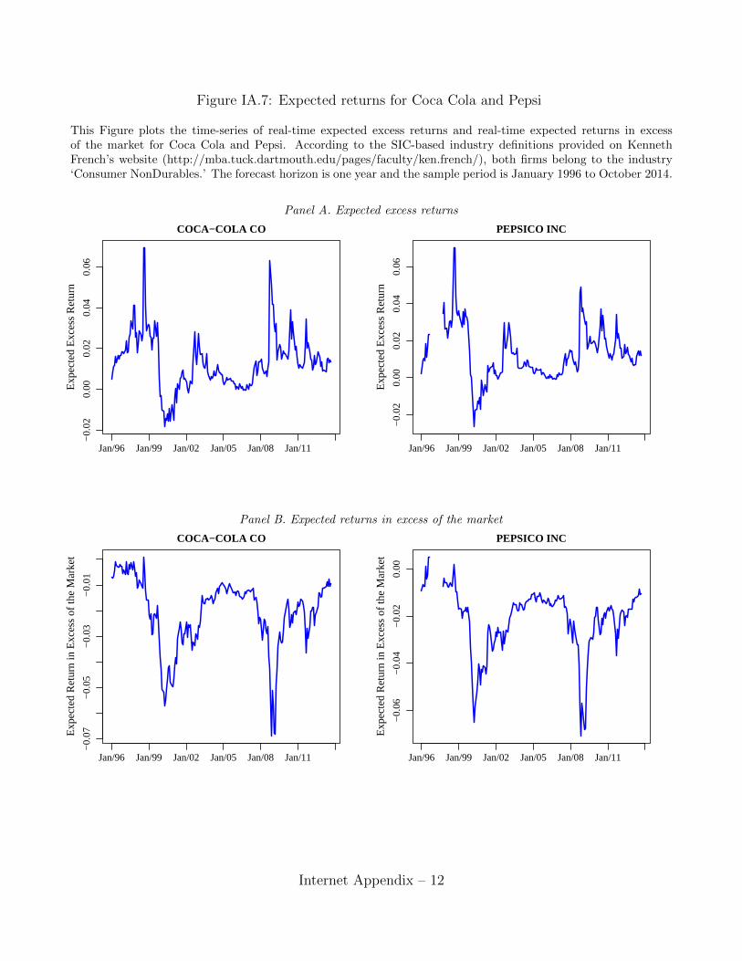
Figure IA.7: Expected returns for Coca Cola and Pepsi

This Figure plots the time-series of real-time expected excess returns and real-time expected returns in excessof the market for Coca Cola and Pepsi. According to the SIC-based industry definitions provided on KennethFrench’s website (http://mba.tuck.dartmouth.edu/pages/faculty/ken.french/), both firms belong to the industry‘Consumer NonDurables.’ The forecast horizon is one year and the sample period is January 1996 to October 2014.


COCA−COLA CO

Exp

ecte

d E

xces

s R

etur

n

−0.

020.

000.

020.

040.

06


PEPSICO INC

Exp

ecte

d E

xces

s R

etur

n

−0.

020.

000.

020.

040.

06



COCA−COLA CO

Exp

ecte

d R

etur

n in

Exc

ess

of th

e M

arke

t

−0.

07−

0.05

−0.

03−

0.01


PEPSICO INC

Exp

ecte

d R

etur

n in

Exc

ess

of th

e M

arke

t

−0.

06−

0.04

−0.

020.

00



what is the expected return on a stock? - centre for finance · what is the expected return on a...

Documents