what influences participation in genetic carrier testing?: results from a discrete choice experiment

Journal of Health Economics 25 (2006) 520–537

What influences participation in genetic carrier testing?Results from a discrete choice experiment

Jane Hall a,∗, Denzil G. Fiebig a,b, Madeleine T. King a,Ishrat Hossain a, Jordan J. Louviere a,c

a Centre for Health Economics Research and Evaluation (CHERE), University of Technology, Sydney,PO Box 123 Broadway, NSW 2007, Australia

b School of Economics, University of New South Wales, Australiac School of Marketing, University of Technology, Sydney, Australia

Received 14 January 2005; received in revised form 13 May 2005; accepted 19 September 2005Available online 21 October 2005

Abstract

This study explores factors that influence participation in genetic testing programs and the acceptanceof multiple tests. Tay Sachs and cystic fibrosis are both genetically determined recessive disorders withdiffering severity, treatment availability, and prevalence in different population groups. We used a discretechoice experiment with a general community and an Ashkenazi Jewish sample; data were analysed usingmultinomial logit with random coefficients. Although Jewish respondents were more likely to be tested, bothgroups seem to be making very similar tradeoffs across attributes when they make genetic testing choices.© 2005 Elsevier B.V. All rights reserved.

JEL classification: D1; I1

Keywords: Genetic testing; Screening; Discrete choice experiments; Stated preferences; Mixed logit

1. Introduction

The possibilities for testing genetic material are increasing rapidly with developments in map-ping the human genome and understanding the role of genes in the development of disease (Yate,1996; Trent, 2000; Trent et al., 2003). One sample of genetic material can be subjected to severaltests, indeed can be stored indefinitely and tested in the future, and genetic abnormalities are

∗ Corresponding author. Tel.: +612 9514 4720; fax: +612 9514 4730.E-mail address: [email protected] (J. Hall).

0167-6296/$ – see front matter © 2005 Elsevier B.V. All rights reserved.doi:10.1016/j.jhealeco.2005.09.002

J. Hall et al. / Journal of Health Economics 25 (2006) 520–537 521

relatively common. Genetic tests can be marketed to healthy people, and so there are medical,public health and commercial interests in promoting their widespread adoption.

Testing programs have generally been evaluated using cost effectiveness analysis of the cost percase prevented. The immediate product of testing, whether diagnostic or screening, is information;and as Berwick and Weinstein (1985) pointed out, the information may have value beyond itsimpact on medical decisions and thereby health outcomes. The value of information, in termsof its direct effect on consumer wellbeing, may be positive or negative. In the case of screeningprograms or testing non-symptomatic individuals, the risk of developing disease may be uncertainand distant in time, and the intervention may be ineffective or carry unattractive side-effects(Cairns and Shackley, 1993). This applies even more strongly to screening using genetic testsas a genetic abnormality does not always imply the certain development of symptomatic diseaseas the possession of a particular gene can indicate a susceptibility to a disease. The informationhas implications for other family members as they share genetic inheritance (Chapple and May,1996).

The extent to which people see genetic testing programs as worthwhile and are prepared to betested depends on how they value the information produced by testing and this in turn is likely tobe related to the severity of the disease, the availability of treatment, and the individual’s risk ofbeing affected as well as how they consider the information will impact on themselves and otherfamily members.

For most screening programs, the information the individual obtains is their individual risk ofdeveloping a particular disease. Testing can also be used to detect abnormalities in an unborn childand has been used where the disease is severe and there is no effective treatment; parents are thengiven the choice of terminating an affected pregnancy (e.g., amniocentesis). With genetic testing,there are implications for family members, as noted above, and also for unconceived children. Forgenetically recessive diseases (that is two copies of the affected gene are required, one inheritedfrom each parent), it is possible to test individuals genetically to detect their carrier status. In thiscase, being identified as a carrier does not imply poorer health outcomes for the individual, ratherit affects their risk of having affected children. This may affect their decisions to marry, or havechildren. The test result may also provide ‘reproductive reassurance’ to couples who discoverthey have no risk of having an affected child.

Economic evaluations of ante-natal testing have accepted the goal of testing programs to bea reduction in the number of people with the disease (Burn et al., 1993; Evans et al., 1995).Most studies have been cost effectiveness analyses, with benefits measured as the number ofaffected births avoided. However, not all women will undergo ante-natal testing, even when offered(Chamberlain, 1978; Piggott et al., 1994). And some women will be tested even though they haveno intention of terminating an affected pregnancy, which has been interpreted as indicating apositive value attached to the information (Mooney and Lange, 1993; Ryan et al., 2003). Indeedthe value of information is generally treated as positive (Stone and Stewart, 1996), although thereare clear negative effects and consequences of a positive screening test, including the feeling ofbeing at risk and vulnerable, the monitoring for disease progression, and potentially feelings ofguilt for passing conditions on to children (Hall et al., 1998).

Genetic testing is easy and non-invasive: a sample can be provided by a mouth swab or a pieceof hair, one sample can be used to test for multiple conditions, and the sample can be stored andre-tested in the future for further conditions. This may encourage people to accept testing whenoffered, and to accept multiple tests. However, there may be community attitudes toward geneticsper se or towards discrimination, which make people less likely to be tested, particularly thosein ethnic or cultural groups who fear stigmatisation. There are also cost implications, as the cost

522 J. Hall et al. / Journal of Health Economics 25 (2006) 520–537

of sample collection is generally much less than the laboratory cost of the test, and the latter isincreased with every additional test. Therefore, what is important in understanding the potentialgrowth of screening programs is individuals’ readiness to take multiple tests when offered.

Thus genetic screening in general, and carrier status screening in particular, provide an inter-esting case for exploring consumer behaviour and the value of information. One approach to thisis to elicit willingness to pay (WTP) for screening. Although contingent valuation is increasinglyused to value the benefits of health programs, there are only three studies (although more papers)which report WTP for genetic screening and these are for ante-natal rather than pre-conceptionalscreening (Miedzybrodzka et al., 1994; Donaldson et al., 1995; Miedzybrodzka et al., 1995;Donaldson et al., 1997; Ryan et al., 2003). The use of discrete choice experiments (DCEs) offersome advantages over the standard contingent valuation approach, particularly when the influenceof several attributes should be considered (Louviere et al., 2000). The one DCE study we haveidentified which investigates preferences for Down’s syndrome screening is also considering ante-natal testing (which carries a risk of miscarriage) and is limited to three attributes (Bishop et al.,2004).

This paper reports the investigation of consumer preferences for testing for carrier status fortwo particular conditions, Tay Sachs (TS) disease and cystic fibrosis (CF). Although both arerecessive, they differ in severity and the availability of treatment, as explained below. Further, theprevalence of these diseases and the awareness of their prevalence and consequences also differby population group and this allows an investigation of the extent to which different cultures andexpectations affect attitudes to screening. This is the first study to apply the DCE approach togenetic testing, and unlike almost all other studies of carrier screening it focuses on the provisionof information prior to conception. A novel feature of this study is to present individuals with thechoice of more than one test, which will increasingly be likely to happen in practice.

The econometric analysis uses the random parameter or mixed logit model (McFadden andTrain, 2000). While becoming an increasingly popular tool for analysts in other disciplines, thereremain unresolved issues in using this technique and, as noted by Fiebig et al. (2005), there havebeen few applications of these methods in health economics. Thus, an important but secondaryaim of the paper is to provide a detailed case study in the specification, estimation and performanceof mixed logit models.

2. Background

Both TS and CF are recessive hereditary disorders. TS is a neuro-degenerative disorder whichresults in progressive neural dysfunction from infancy, and death, usually by 5 years of age(Kaback et al., 1993). TS is most prevalent in the Ashkenazi Jewish population (Jewish individualsof Eastern European descent), with carrier rates of 1 in 25 compared to 1 in 250 in the generalpopulation. Within this population group, a high awareness of the risks and consequences of TS hasled to well established programs to reduce its incidence. CF varies in severity and is usually fatalby the age of 30. Individuals with CF experience a higher number of respiratory infections thannon-affected individuals, leading to developmental difficulties and periods of handicap. In severecases of CF, individuals lack control of their motor functions and have poor mental development.In less severe cases, they function apparently well without difficulty or assistance. Carrier rates inthe general Australian population have been estimated at between 1 in 20 and 1 in 25 (Wake et al.,1996). There is no prevention for either condition and no efficacious treatment for TS. However,developments in treatments for CF mean that while a cure is not possible, the quality and lengthof life of CF sufferers has improved.


Testing for both TS and CF carrier status is possible. In New South Wales, Australia, TStesting prior to conception is currently offered through Jewish community hospitals, or through aspecialised laboratory. CF testing is offered generally through obstetric care. While CF tests canbe performed pre-natally, it is often tested post-natally, although it may affect future reproductivechoices of the couple. Population screening for both TS and CF jointly is also offered through ahigh school program in selected schools. When individuals rather than couples are tested, theyreceive their results as individuals soon after testing, or elect to receive results later as an individualor as a couple.

There have been a number of economic evaluations of testing for TS and CF. Most of these arecost effectiveness analyses, with the number of births avoided as the measure of benefits. In somestudies (Burn et al., 1993; Evans et al., 1995), the costs of caring for afflicted children (additionalhealth care, special education, institutional care and/or home support) have been estimated andcompared with the costs of testing and subsequent abortions. Some studies (Hagard and Carter,1976; Henderson, 1982; Gill et al., 1987) have used a human capital approach to estimating thevalue of benefits, allowing for the marketable output of the mother and any replacement childrenas an estimate of the value of preventing the birth of a handicapped child.

Whilst the use of contingent valuation offers a method of avoiding this restriction on what rangeof benefits are considered, there are only two published related studies which have attemptedto do this for CF; in one respondents were women who had been tested and had a negativeresult (Donaldson et al., 1995); and in the other, women attending the same ante-natal clinic ata later time but who were not offered testing (Donaldson et al., 1997). Both these attempted tocompare alternative testing strategies (individuals versus couples). The first study showed verylittle difference in mean WTP between the two alternatives. This is not surprising if WTP isinfluenced more by the willingness to be tested, than by differences in the testing strategy; and soprovides little information about the decision to be tested. The second paper did report statisticallysignificant differences between WTP for the two strategies, with a higher WTP for couple testingalthough most respondents stated a preference for individual testing. The authors commented thatthis was probably due to respondents’ perception of the higher cost of providing couple testing.

3. Stated preference methods

Stated preference data can be useful where market or revealed preferences do not exist, as isthe case for many health programs and innovative treatments. There are various ways of elicit-ing stated preference data, one of which is discrete choice experiments. This approach requiresrespondents to make choices over hypothetical but realistic alternatives rather than ranking orrating. Treatments or programs are described in terms of their underlying attributes (consistentwith Lancastrian consumer theory), and the alternatives are constructed by varying each attributeover a range of levels. A sample of alternatives is selected from the combination of all possibleattribute levels using experimental design principles. Typically, each respondent is presented withseveral choice scenarios, thus contributing multiple observations (for more detail and explanationsee (Fiebig and Hall, 2004).

4. Development of attributes

Attributes were selected initially from a review of the literature on individuals’ attitudes togenetic testing and consultation with clinicians involved in testing programs. We hypothesisedthat the attributes of the testing program and the characteristics of the individuals both influence


attitudes. For TS, being of Jewish descent is important (as TS has a higher incidence in theAshkenazi Jewish population). For this reason, we conducted qualitative research into attitudestowards genetic testing in the Jewish community, as reported elsewhere (Haas et al., 2001). Thisexpanded the number of attributes considered.

Attribute levels were selected to be realistic in terms of available technology and screeningprograms. Attributes and levels were tested in a pilot study, involving one sample of 25 respondentsfrom the general community and one sample of 27 from the Jewish community. Eligibility criteriaand recruitment methods for the pilot study were as for the main study (detailed below). The pilotinterviews were carried out by a market research firm. Most people in the pilot chose to be testedfor both conditions most of the time. Therefore, the range of attribute levels was expanded toencourage more variability in responses. The final list of attributes and levels is shown in Table 1.

5. Experimental design

Nine attributes with four levels and three attributes with two levels yield 23 × 49 (over 2 million)possible combinations. A systematic sample of scenarios was selected from the complete factorialusing an orthogonal, fractional factorial design, according to the principles given in (Viney et al.,2005). This design contains 512 scenarios in which all attribute main effects (12) and eight of thepossible (66) two-way interactions were orthogonal to each other and independently estimable.

5.1. The questionnaire

The pilot study demonstrated that people generally understood the material and could handlea survey consisting of 16 scenarios. To cover the 512 scenarios with each respondent seeing16, required 32 different versions of the questionnaire. All attribute levels appeared with equalfrequency in each version. Recruits were assigned randomly to version. One attribute varied howpeople received the test results; either as their individual results or as a couple (remembering thatboth these conditions require two carrier parents for an affected child). For respondents who weresingle, there was an alternate version of the questionnaire, which clarified that receiving resultsas a couple would be in the future. Respondents were offered four options, or alternatives, in each

Table 1Attributes and levels

Attributes Levels

Whether your doctor recommends you have a test Yes; noWhether you are told your carrier status as an individual or whether

you are told your risk as a coupleIndividual; couple

Where you go to be tested Any doctor; specialised clinicThe chance that you are a carrier even if the test is negative 15; 30; 45; 60%Time waiting for results 24 h; 1 week; 1 month; more than 1 monthCost to you of being tested for TSD $0; $150; $300; $600Cost to you of being tested for CF $0; $375; $750; $1500Risk of being a carrier for TSD 1:25; 1:250; 1:2500; 1:25,000Risk of being a carrier for CF 1:25; 1:250; 1:2500; 1:25,000The risk that a child born with CF will experience mild symptoms

compared to severe case20; 40; 60; 80%

Proportion of people like you who have been tested for TSD 20; 40; 60; 80%Proportion of people like you who have been tested for CF 20; 40; 60; 80%


scenario: to choose whether they would be tested for CF only, TS only, both together, or not havetesting. A scenario from the questionnaire is provided in Appendix A.

The questionnaire was designed for self-completion, and the 16 scenarios were preceded by aone-page information sheet describing relevant details about the two diseases and the screeningconditions, and a series of questions designed to provide a profile of each respondent. Thesequestions included sociodemographic variables, current family situation and plans for havingchildren, whether the respondent had known anyone with Tay Sachs or cystic fibrosis, and whetherthey ever had genetic testing. A copy of the questionnaire is available from the authors on request.

6. Recruitment and data collection

Two samples were recruited by a market research firm, one from the general community andone from the Jewish community. The eligibility criteria were that respondents were over 18 yearsof age and could read and understand English. The general community sample was recruited door-to-door in a random sample of suburbs across the Sydney metropolitan area; respondents weregiven an adult ticket to a movie. Jewish respondents were also from Sydney, recruited throughJewish community and religious organisations, after contact and discussion by the research teamwith community and religious leaders. There is an active testing program for Tay Sachs promotedthrough the same Jewish community groups. The incentive to participate was not an individualbenefit, as in the case of the general community sample, but a cash benefit of $20 AUD perparticipant paid to the community group through which they were recruited. This was based onthe market research firm’s experience, that for this method of recruitment, participation is improvedwhen the respondent feels their involvement benefits their community group. All interviews wereconducted in participants’ home by an experienced interviewer, who explained the survey, obtainedinformed consent, and went through the information sheet and questionnaire with the respondent.

7. Econometric analysis

7.1. Mixed logit choice model

The statistical analysis of choice data relies on the random utility model (McFadden, 1981)where each respondent faces a choice amongst j alternatives repeated under s scenarios or choicesituations. While the Jewish and general population samples were analysed separately, the mod-elling framework is the same. The utility that individual i derives from alternative j in scenario sis composed of systematic and random components denoted by

Uisj = X′isjβi + εisj (1)

where Xisj is a K × 1 vector of explanatory variables and βi is a conformable vector of coefficients.Conditional on βi, and assuming the disturbance terms εisj to be identically and independently

distributed (IID) as extreme value, the standard multinomial logit (MNL) specification results.The probability that individual i chooses j in scenario s is then given by

Pisj = exp (X′isjβi)

∑hexp (X′

ishβi)(2)


A generalisation of the MNL specification that allows for possible heterogeneity amongst indi-viduals involves setting

βki = Z′iβ̄k + σkωki, k = 1, . . . , K (3)

where Zi is a vector of observed characteristics of respondent i, the β̄k are parameter vectors and�kωki represents unobserved heterogeneity in the preference weights. In its simplest form withZi = 1, (3) yields a standard random coefficient specification. The ωki are assumed to follow stan-dard normal distributions, independent of each other and of the εisj. Notice that this specificationallows βki to vary over individuals, but not over the repeated choices made by that individual.Error correlation is thus introduced across choice situations, accounting for the panel structure ofthe data. This correlation is not perfect because of the presence of the independent extreme valueterms εisj. Even though the ωki are assumed to be independent, this specification also inducescorrelation across alternatives as long as generic attributes appear in the utility specifications forthese alternatives.

The resultant random parameter or mixed logit (MXL) model has recently become very popularin empirical work, providing a flexible and computationally practical discrete choice specification;see for example Brownstone and Train (Revelt and Train, 1998; Brownstone and Train, 1999;Layton and Brown, 2000; McFadden and Train, 2000). Estimation by maximum simulated like-lihood (MSL) is undertaken using a program downloaded from Kenneth Train’s website (Train,2004). All estimation results reported below were generated using 1000 Halton draws to simulatethe likelihood functions to be maximised (Train, 2003).

7.2. Model specification

In each of 16 choice tasks, the respondent is asked to choose between four different alternatives.For each of the three screening alternatives: test for CF only (j = CF), test for TS only (j = TS), testfor both (j = BOTH), the utility that individual i receives from alternative j in scenario s is givenby

Uisj = X′1isjβ1ij + X′

2isjβ2i + X′3isjβ3ij + X′

4isjβ4ij + Z′iβ5 + εisj, j = CF, TS, BOTH

(4)

The fourth (j = 0) alternative allows the individual to choose not to have any tests. The associatedutility is normalised to zero. In (4), the attributes manipulated in the choice experiment have beendivided up according to whether they are alternative-specific, X1, or generic and hence appear inthe utilities associated with all of the testing alternatives with the same coefficient, X2, or whetherthey appear only in TS and BOTH, X3, or only in CS and BOTH, X4. The demographic variables,Z, serve to shift any alternative-specific intercepts for the testing alternatives, and hence representtendencies to test relative to not testing.

McFadden and Train (McFadden and Train, 2000) provide strong theoretical support for MXLwhen they prove that any well-behaved random utility model can be approximated to any spec-ified degree of accuracy by a MXL model. Unfortunately this existence result does not lessenthe practical problem of deciding what particular specification should be chosen. Further, it isimportant to recognise that the richer stochastic structure that results from the random parameterframework of MXL is a by-product of the model specification and simple changes in the specifi-cation of the systematic component of (1) may have major implications for the resultant stochasticstructure.


Consider the treatment of alternative-specific intercepts in this model. The standard approachwould be to include separate intercepts for each of the testing alternatives; call this specificationM1. Rewriting (1) so that Xisj is partitioned in order to separate out the intercepts from theremaining vector of explanatory variables denoted by Aisj, M1 would be given by

Uisj = αij + A′isjβi + εisj, j = CF, TS, BOTH (5)

Alternatively one could specify a generic testing intercept and allow for two alternative-specificshift dummies; call this specification M2. If DC is a dummy variable indicating CF and DB adummy variable indicating BOTH then M2 can be written as

Uisj = δ0i + DCisjδ1i + DBisjδ2i + A′isjβi + εisj, j = CF, TS, BOTH (6)

In an MNL framework without random parameters the choice between M1 and M2 is simplyabout ease of interpretation and both models will produce identical inferences.

Suppose now we move to our MXL framework where the intercepts are assumed random.M1 will induce heteroskedasticity but not correlation across alternatives and, for each individual,correlation between the utilities of a particular choice. While M2 will allow for this form ofheterogeneity in the covariance structure, the presence of the random component associated withthe common testing variable will also induce correlation across alternatives that is not presentin M1. These two model specifications were estimated as intermediate steps to facilitate ourunderstanding of the sources of heterogeneity in our data due to relationships within individualsand between choices.

8. Results

Completed questionnaires were returned from 210 respondents from the Jewish community,and 261 respondents from the general community. The sample sizes used in estimation are con-siderably larger because each respondent answered 16 scenarios. These are also comparable withother applications of MXL. Descriptions of the demographic variables, and their coding in themodel estimation, are given in Table 2. The sociodemographic profile of the Jewish sample wasmore homogeneous than that of the general population: Jewish respondents were more educated,had higher incomes, and included a higher proportion of women and younger people with plans

Table 2Demographic variables, coding and sample means and percentagesa

Variable and coding for model estimation Jewish General population

Continuous variablesAge = age in years 33 43Income = household income in $’000 s pa 97 61

Dummy variablesWanting to have more children, kids more = 1 if yes 53 27Level of education completed, Educ low = 1 if low or mid education 14 46Completed vocational or trade certificate, Educ voc = 1 if vocational education 4 15Completed University diploma/degree, Educ high = 1 if high education 82 39Income not reported, incmsg = 1 if missing income 10 8Marital status: single, single = 1 if single 50 34

a All dummy variables have been effects coded in the estimation results and Educ high is the omitted base category foreducation.


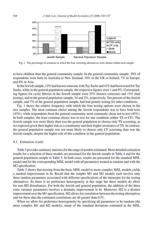
Fig. 1. The percentage of scenarios in which the four screening alternatives were chosen within each sample.

to have children than the general community sample. In the general community sample, 70% ofrespondents were born in Australia or New Zealand; 10% in the UK or Ireland; 7% in Europe;and 8% in Asia.

In the Jewish sample, 12% had known someone with Tay Sachs and 41% had been tested for TaySachs, while in the general population sample, the respective figures were 1 and 0%. Correspond-ing figures for cystic fibrosis in the Jewish sample were 25% (known someone) and 13% (hadtesting), and in the general population sample, 34 and 2%, respectively. Ten percent of the Jewishsample, and 7% of the general population sample, had had genetic testing for other conditions.

Fig. 1 shows the relative frequency with which the four testing options were chosen in thetwo samples. The most common choice among the Jewish respondents was to have both tests(43%), while respondents from the general community most commonly chose not to test (45%).In both samples, the least common choice was to test for one condition (either TS or CF). TheJewish sample was more likely than was the general population to choose only TS screening, aswe expected given their higher risk as a community and their higher awareness of TS. In contrast,the general population sample was not more likely to choose only CF screening than was theJewish sample, despite the higher risk of this condition in the general population.

8.1. Estimation results

Table 3 provides summary statistics for the range of models estimated. More detailed estimationresults for a selection of these models are presented for the Jewish sample in Table 4 and for thegeneral population sample in Table 5. In both cases, results are presented for the standard MNLmodel and for the corresponding MXL model with all parameters treated as random and with theM2 specification.

Table 3 shows that moving from the basic MNL model to more complex MXL models yieldsa marked improvement in fit. Recall that the simpler M1 and M2 models each involve onlythree random parameters associated with different specifications of the intercepts for the testingalternatives. So there is no preference heterogeneity at this stage but these models do allowfor non-IID disturbances. For both the Jewish and general population, the addition of the threeextra variance parameters involves a dramatic improvement in fit. Moreover, M2 is a distinctimprovement over the M1 specification. M2 allows for correlation between the testing alternativesand for these data the estimated correlations are all greater than 0.53.

When we allow for preference heterogeneity by specifying all parameters to be random (themore complex M1 and M2 models), many of the standard deviations estimated in the MXL


Table 3Summary statistics for alternative models

MNL Mixed logit

Only intercepts random All coefficients random

M1 M2 M1 M2

Ashkenazi JewishPseudo R2 0.1171 0.2875 0.3127 0.3507 0.3598AIC 7450 5993 5784 5519 5443BIC 7664 6225 6011 5904 5829LR test 524.42 391.02

General populationPseudo R2 0.0948 0.3032 0.3397 0.3693 0.3814AIC 9046 6986 6623 6381 6260BIC 9268 7227 6864 6780 6660LR test 655.48 413.02

Notes: Pseudo R2 is defined as 1 − (LL/LL0), where LL is the value of the (simulated) log-likelihood function evaluatedat the estimated parameters while LL0 is the value of the log-likelihood function for a base model that only containsa non-random alternative-specific intercepts. AIC is −2(LL − M) and BIC is −2LL + M ln N where M is the number ofparameters and N the number of observations. LR test is the conventional likelihood ratio test for the null hypothesisthat the variances associated with random parameters of attributes (not including the intercepts) are all zero. (See text forfurther discussion.).

framework are large and statistically significant. As measured by the pseudo R2’s, there is anadditional improvement in fit compared to the simpler M1 and M2 models although now thereare an additional 25 parameters to be estimated. The AIC and BIC criteria indicate that thisimprovement remains after penalizing for the loss of parsimonious specification. This indicatesthe presence of considerable preference heterogeneity and vindicates the move away from the basicMNL model and the simpler MXL specifications. While these models are nested, the hypothesistests are non-standard because the parameter space is restricted under the alternative. In suchsituations the LR test statistic does not have the usual chi-square asymptotic distribution (Andrews,1998). In this case the appropriate critical value will be smaller than the usual chi-square value, andthe large log-likelihood difference reported for the comparisons of the simpler M1 and M2 modelswill lead to rejecting these in favour of the full MXL models at every reasonable significance level.

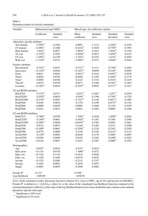
Table 4 presents the results for the Jewish sample. Respondents were more likely to test withhigher risk of disease (both Tay Sachs and cystic fibrosis), as the accuracy of testing improved,when their doctor recommended testing, when the test was only available at a specialised clinic,and as the price decreased. Planning to have more children also made respondents more likely toaccept testing. Moving to a discussion of the specific parameter estimates, note that comparisonsof the MNL and MXL estimates require some care. If, in fact, the latter is the more appropriatespecification, then the parameter estimates and standard errors are not strictly comparable forthe following reason. In the MXL model, the parameter estimates are normalised relative to theextreme value part of the disturbance term, that is, net of the error component introduced by therandom coefficients. Since the disturbance in the MNL specification captures both sources oferror, it will have a larger variance and hence normalisation relative to this variance will lead toestimated parameters that can be expected to be smaller than those of the MXL. This is reflectedin Table 4; the MNL coefficients are typically smaller in magnitude than the MXL coefficients.


Table 4Estimation results for Jewish community

Variables Multinomial logit (MNL) Mixed logit, all coefficients random

Coefficient Standarderror

Meancoefficient

Standarderror

Standarddeviation

Standarderror

Alternative specific attributesTest dummy 0.7945** 0.2564 0.8051 1.1131 2.3428** 0.2576CF dummy −0.2901** 0.1060 −0.4234** 0.1836 0.7799** 0.1993Both dummy 1.5022** 0.0877 2.8838** 0.1843 1.3910** 0.1538TS cost −2.5336** 0.2407 −4.9840** 0.5013 1.8299** 0.6142CF cost −1.4503** 0.1359 −3.3225** 0.3193 1.4315** 0.3018Both cost −1.2158** 0.0733 −3.4883** 0.2721 3.0446** 0.3644

Generic attributesRecommend 0.3333** 0.0437 0.7371** 0.1111 0.7706** 0.1692Inaccuracy −0.1230** 0.0264 −0.1453** 0.0698 0.5145** 0.0492Form 0.0617 0.0442 0.3615** 0.1419 0.8395** 0.2078Time1 0.0020 0.0764 −0.0448 0.1393 0.3665** 0.1779Time7 0.0505 0.0746 0.1222 0.1332 0.2518* 0.1419Time30 0.0274 0.0756 0.0271 0.1568 0.5367** 0.1967Location −0.1283** 0.0434 −0.3547** 0.0943 0.3717** 0.1417

TS and BOTH attributesRiskTS25 0.7179** 0.0717 1.8253** 0.1687 1.2257** 0.2544RiskTS250 0.2970** 0.0676 0.5494** 0.1396 0.7399** 0.1702RiskTS2500 −0.2756** 0.0653 −0.7327** 0.1149 0.4073** 0.1885PropTS40 0.0169 0.0676 0.1759 0.1299 0.6575** 0.1762PropTS60 −0.0080 0.0670 −0.0883 0.1049 0.1310 0.1659PropTS80 0.0162 0.0673 0.0941 0.1092 0.0890 0.1698

CF and BOTH attributesRiskCF25 0.7488** 0.0709 1.7904** 0.1838 1.0598** 0.2045RiskCF250 0.1569** 0.0667 0.3926** 0.1287 0.3386 0.2098RiskCF2500 −0.2096** 0.0658 −0.6493** 0.1385 0.0403 0.2601PropCF40 0.0714 0.0672 0.1248 0.1203 0.3213 0.2380PropCF60 −0.1099* 0.0661 −0.2584** 0.1218 0.2165 0.2550PropCF80 0.0770 0.0688 0.1348 0.1226 0.4314** 0.2115SeverCF20 0.1358** 0.0683 −0.0244 0.1170 0.3805* 0.2097SeverCF40 −0.0104 0.0669 0.0107 0.1262 0.4300* 0.2434SeverCF60 −0.0144 0.0667 0.1657 0.1267 0.5089** 0.1592

DemographicsAge −0.0297 0.0516 0.3197 0.2619Kids more −0.1176 0.0736 1.1008** 0.3472Educ low −0.1738 0.1143 −0.1815 0.4540Educ voc 0.1220 0.1685 −0.0139 0.4933Income −0.1335 0.1085 −0.2151 0.7357Incmsg 0.1026 0.0952 0.2639 0.2957Single −0.0901 0.0655 −0.2948 0.3882

Pseudo R2 0.1171 0.3598Log-likelihood −3689.89 −2658.58

Notes: In the estimation results, inaccuracy has been scaled in 10’s, costs in 1000’s, age in 10’s and income in $100,000’s.Pseudo R2 is defined as 1−(LL/LL0), where LL is the value of the (simulated) log-likelihood function evaluated at theestimated parameters while LL0 is the value of the log-likelihood function for a base model that only contains a non-randomalternative-specific intercepts.

* Significant at 10% level.** Significant at 5% level.


Table 5Estimation results for general population

Variables Multinomial logit (MNL) Mixed logit, all coefficients random

Coefficient Standarderror

Meancoefficient

Standarderror

Standarddeviation

Standarderror

Alternative specific attributesTest dummy −1.7338** 0.1731 −3.9313** 0.9565 3.3136** 0.2567CF dummy 0.2094** 0.1046 0.4607** 0.1788 0.5460** 0.1671Both dummy 1.4781** 0.0926 2.4142** 0.2507 1.9501** 0.1918TS cost −1.1336** 0.2441 −2.6315** 0.5168 1.2753* 0.7476CF cost −0.7474** 0.1054 −1.7804** 0.2185 0.7224** 0.1213Both cost −0.5195** 0.0629 −1.6172** 0.1908 1.3161** 0.1715

Generic attributesRecommend 0.3830** 0.0352 1.0222** 0.1353 1.1621** 0.1529Inaccuracy 0.0262 0.0211 0.0858 0.0631 0.4382** 0.0594Form 0.0666* 0.0351 0.1137 0.0926 0.7271** 0.1238Time1 −0.0364 0.0613 −0.0155 0.1274 0.5413** 0.2139Time7 −0.0435 0.0598 0.0375 0.1209 0.1209 0.1713Time30 0.1606** 0.0616 0.1215 0.1412 0.0914 0.3972Location −0.2027** 0.0350 −0.5305** 0.0794 0.3540** 0.1502

TS and BOTH attributesRiskTS25 0.5815** 0.0573 1.4696** 0.1403 1.2779** 0.1755RiskTS250 0.2802** 0.0572 0.5822** 0.1214 0.3828 0.2995RiskTS2500 −0.2706** 0.0604 −0.6534** 0.1236 0.7328** 0.1262PropTS40 −0.0044 0.0591 −0.0324 0.0951 0.0484 0.1442PropTS60 0.0638 0.0580 0.0887 0.1164 0.5849** 0.2256PropTS80 0.0557 0.0604 0.2622** 0.1144 0.0872 0.1278

CF and BOTH attributesRiskCF25 0.5471** 0.0581 1.4149** 0.1681 1.4013** 0.1831RiskCF250 0.2772** 0.0568 0.5190** 0.1216 0.9848** 0.1673RiskCF2500 −0.2584** 0.0611 −0.6212** 0.1302 0.4466** 0.2028PropCF40 −0.1619** 0.0594 −0.3467** 0.1074 0.0229 0.1674PropCF60 0.0752 0.0579 0.0378 0.1083 0.2319 0.3253PropCF80 0.1324** 0.0596 0.3201** 0.1369 0.2698 0.2410SeverCF20 0.0347 0.0593 0.1017 0.1157 0.1713 0.3301SeverCF40 −0.0833 0.0591 −0.0687 0.1316 0.5459** 0.1063SeverCF60 −0.0432 0.0592 −0.0221 0.1061 0.0563 0.1584

DemographicsAge −0.0363 0.0270 0.0050 0.1928Kids more 0.2417** 0.0500 0.8167** 0.2300Educ low −0.1213** 0.0519 −0.4514** 0.2128Educ voc 0.3752** 0.0663 1.4330** 0.3080Income 0.5191** 0.0983 1.8659** 0.4747Incmsg −0.3900** 0.0740 −1.5111** 0.3651Single −0.2629** 0.0402 −0.6042** 0.1733

Pseudo R2 0.0948 0.3814Log-likelihood −4487.91 −3067.18

Notes: In the estimation results, inaccuracy has been scaled in 10’s, costs in 1000’s, age in 10’s and income in $100,000’s.Pseudo R2 is defined as 1 − (LL/LL0), where LL is the value of the (simulated) log-likelihood function evaluated atthe estimated parameters while LL0 is the value of the log-likelihood function for a base model that only contains anon-random alternative-specific intercepts.

* Significant at 10% level.** Significant at 5% level.


Because the stochastic portion of utility has different variances in the two models, it is difficult tocompare the magnitude of coefficient estimates, but signs can be compared. Coefficient estimatestypically have signs that are consistent with a priori expectations. Moreover, they are consistentacross models. Many of the standard deviations estimated in the MXL framework are large,statistically significant and have magnitudes that are also sensible.

When mean coefficients are precisely estimated the associated standard deviations are oftenalso precisely estimated but less in magnitude than the estimated mean coefficient. The cost and,to some extent, the risk of TS and CF attributes are prime examples of this pattern. Often in mixedlogit estimations the price/cost effect is assumed to be fixed a priori (Revelt and Train, 1998; Laytonand Brown, 2000). One rationale is to avoid distributions of price effects that include positiveresponses or to avoid identification problems. In our work, there were no convergence problemswith this particular suite of models and when cost is given a random coefficient the associatedstandard deviations are often highly significant. While this provides evidence of heterogeneityin these responses, the implied estimated distribution for these random parameters have onlyrelatively small probabilities associated with parameter values that have signs different from themean. Consequently, there seems little to be gained by specifying fixed price effects.

There are some cases of precisely estimated mean coefficients and standard deviations butwhere the standard deviations are quite large relative to the magnitude of the mean. Notableexamples of this pattern are inaccuracy and form and to some extent recommendation and location.The implication is that there is considerable diversity in the way people value these attributes andin particular there are substantial proportions of people whose utility weighting differs in signfrom the sign of the estimated mean.

In a similar vein, the effects associated with waiting time for test results and the severity ofCF have small and insignificant estimated means but have relatively large and precisely estimatedstandard deviations. Again there is considerable heterogeneity in how these attributes impact onscreening but on average the effects are small.

There are a number of attributes that have small and insignificant estimated means and standarddeviations. For these data these characteristics seem to have little effect on screening behavioureither in terms of people’s tendency to screen or the variability of their screening choices. Includedin this group of attributes is proportion of people tested for TS and the proportion of people testedfor CF.

With the exception of the positive effect that an intention to have more children has on testing,none of the demographic affects are individually, precisely estimated for the Jewish sample.

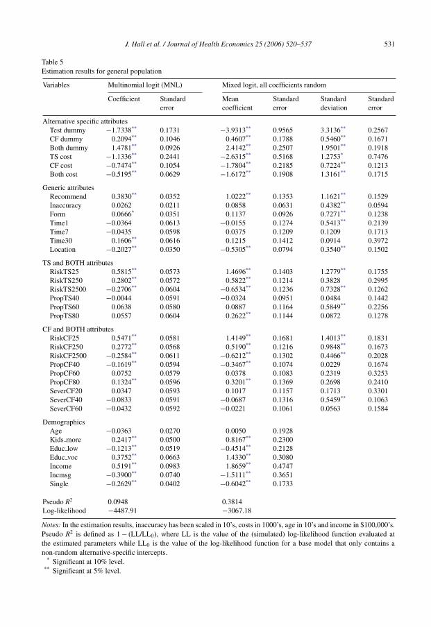
Results for the MXL model for the general population are presented in Table 5. The effectsare similar, with respondents more likely to test as their risk of disease increased, when theirdoctor recommended testing, when the testing was offered at a specialised clinic, and as pricedecreased. Being married, planning to have more children, higher incomes and higher educationalso increased the probability of accepting testing. As in the case of the Jewish sample, the signs ofthe coefficients are typically sensible and a large number of mean effects and standard deviationsare precisely estimated. In fact the pattern of the results is remarkably similar across the twosamples. There is no reason why this should occur and indeed separate samples were collected inorder to identify any differences. However, one usually needs to be careful in comparing estimatesacross samples in discrete choice models because differences in error variation may occur thattranslate to differences in the scale of parameter estimates.

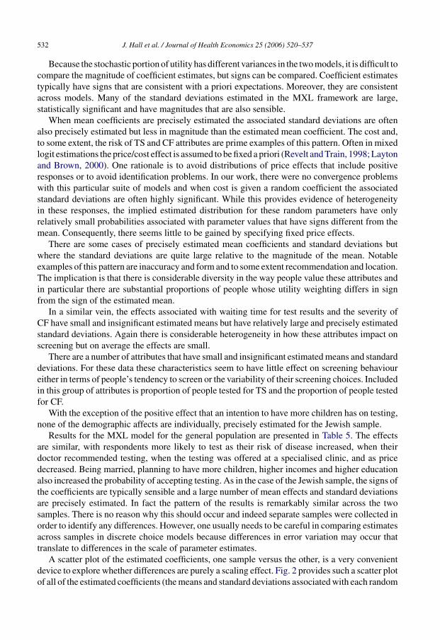
A scatter plot of the estimated coefficients, one sample versus the other, is a very convenientdevice to explore whether differences are purely a scaling effect. Fig. 2 provides such a scatter plotof all of the estimated coefficients (the means and standard deviations associated with each random


Fig. 2. Comparison of general population and Jewish MXL estimates.

coefficient) from the Jewish and general population samples. With a few notable exceptions, theplot confirms the similarity of the coefficient estimates. Further, the strong linear relationshipindicates that differences in coefficient magnitudes are largely explained by differences in scaleassociated with the two samples. The primary exception is the testing intercept that reflects theinherent differences in the tendency to test by the two different groups. This is to be expectedand investigation of scaling phenomena would typically exclude consideration of the alternativespecific intercepts in any formal comparison (Swait and Louviere, 1993; Louviere et al., 2000).Removing the testing intercept estimate and the associated estimated standard deviation leads toan increase in the correlation between the two sets of estimates from 0.68 to 0.82.

While not a difference that is picked up by Fig. 2, the other main difference in the results isthat many of the demographic variables are precisely estimated for the general population. Justas in the Jewish sample, people from the general population who expressed an intention to havemore children were much more likely to test. However, for the general population there were alsosignificant effects for education, income and marital status. Those with more education were morelikely to test, as were those with higher incomes and who were married. For the general population,the introduction of these significant demographic effects serves to reduce the variability associatedwith the random alternative specific intercepts.

9. Discussion

In these two samples, there was a high acceptance of testing with most people choosing tohave either one or both tests in most situations; and respondents were more likely to be tested forboth conditions than only one. In general terms, this indicates the potential demand for the typeof information provided by genetic testing. The policy implication of this, particularly in healthcare systems with predominantly public funding and few out-of-pocket costs to consumers, isthat genetic testing could generate substantial additional costs. To what extent widespread testingwould represent an improvement in social welfare is more difficult to ascertain. Willingness topay estimates for testing can provide some indication of the value consumers place jointly ontheir perception of health benefits and information.

There was evidence of considerable diversity among individuals in the value they attached tosome attributes, with some people considering them as positive contributions to utility while oth-


ers saw the same attributes as negative. This suggests two things: that the common interpretationof “the more information the better”, always providing positive value, is over-simplistic; and thatinformation may carry both positive and negative consequences. This accords with the earlierfindings of (Berwick and Weinstein, 1985) in the context of ante-natal ultrasound. Further investi-gation of the value of information is warranted, particularly in the context of genetics. Informationhas value beyond the individual, for example genetic information may affect employment andinsurance, and this in turn may be both positive and negative. There may indirect effects on levelsof discrimination more generally, and on social attitudes to disability. So individual willingnessto pay for individual information is unlikely to capture the broader social effects (Hall, 1996).

Jewish respondents were more likely to be tested, and more likely to select TS testing, thanthe non-Jewish respondents. This is not surprising given the greater awareness of the risk andthe consequences of this disease in the Jewish community. Jewish communities have adopted,long before the possibility of genetic testing, strategies to select marriage partners to reducethe probability of affected children. Preventing cases is seen as part of the religious duty ofhealing (Levin, 1999). In our earlier qualitative study, one of the reasons for testing profferedwas that a good community member did test, and being tested was part of one’s responsibilityto the community (Haas et al., 2001). It was interesting, then, that the attribute representing theproportion of other people like the respondent tested was not found to be significant. This doesnot necessarily mean that community influences are unimportant; it could indicate an adherenceto what is believed to be right irrespective of others’ behaviour.

An unexpected result is that respondents preferred to be tested at a specialised clinic. Testingavailability at any doctor or clinic was hypothesised to offer more convenience and involve lesstravel time than having to visit a specialised clinic. This hypothesis was not suggested to therespondents. Rather than considering convenience, it may be that respondents interpreted thelatter as offering a higher quality service such as other specialised services, which they prefer inthe context of genetic testing, and this may explain the result.

Both Jewish and general population respondents preferred to receive information as a couplebut the mean effect was not statistically significant for the latter. What is consistent across thetwo samples is that there was considerable heterogeneity in how this attribute was valued; bothestimated standard deviations were large (relative to the estimated mean) and precisely estimated.This type of heterogeneity may explain some of our results. Previous explanations relying onrespondents’ perception of higher costs of providing couple testing are not appropriate in ourwork because of the independent variation of cost in the experimental design.

In the general population results, several demographic factors emerged as significant determi-nants of testing choice. This was not the case with the Jewish sample, but the sociodemographichomogeneity of this group (relative to the general community sample) is the likely reason for thisdifference. The one effect that emerged as significant in both samples was whether respondentsexpressed an intention to have more children. This suggests that when people are planning fami-lies, they place extra value on prenatal genetic information and hence are more likely to participatein genetic testing for CF and TS.

The similarity of the coefficient estimates for testing attributes across the two samples is aninteresting result, and one we did not expect given the cultural and sociodemographic differencesbetween the two samples. With the exception of the testing intercept (that reflects the inherentdifferences in the tendency to test by the two groups), differences in the coefficients across thetwo samples seem to be only due to scale differences. Thus, members of the Jewish and generalpopulations seem to be making very similar tradeoffs across attributes when they make genetictesting choices.


That the general population coefficients tend to be systematically smaller than the correspond-ing Jewish coefficients indicates more inherent variability in the general population results. Suchan outcome is consistent with the greater sociodemographic homogeneity in the Jewish sampleand the fact that they are more familiar with genetic testing. From a modelling perspective, thisresult highlights the need to differentiate different sources of heterogeneity when modelling datafrom discrete choice experiments. Preference heterogeneity can be accounted for by allowing forrandom parameters but there may be other sources of heterogeneity that need to be explicitlyrecognised.

The generalisability of our conclusions and the extent to which truly representative sampleswere obtained warrants some consideration given our recruitment methods. This is particularlytrue of the Jewish sample, where recruitment relied on volunteers from religious and communityorganisations in Sydney where screening for Tay Sachs has been actively promoted for someyears. We have shown that our samples did not contain a preponderance of people with interest inand prior knowledge of genetic screening generally and Tay Sachs or cystic fibrosis specifically.Further, the consistency of our findings across both samples, though not expected a priori, maysuggest some commonalities in attitudes to genetic screening that are worth exploring in futureresearch.

This research raises two issues for consideration in further evaluations of screening programs.First, participation in screening programs is frequently lower than the targets set. Modellingthe factors that influence participation can ensure that screening programs are designed to meetparticipation targets. Second is the question of what constitutes the appropriate measure of benefitfor screening programs. Limiting these to health outcomes (cases detected, cases prevented,or even QALYs) ignores other aspects of screening that individuals value. Conceptualising theproduct of screening as information is a useful start, but understanding the value of informationis complex. Information can simultaneously have positive and negative consequences, geneticinformation carries externalities, and there may be considerable differences across individuals inhow they value these consequences. Broader conceptualisations of benefit and more sophisticatedapproaches to accounting for heterogeneity in population preferences are required for evaluationsto reflect social welfare.

Acknowledgments

This study was supported in part by a National Health and Medical Research Project Grantand in part by a National Health and Medical Research Program Grant. We would like to thankMarion Haas, Patsy Kenny and Richard de Abreu Lourenco for their work on the pilot for thisstudy and Richard de Abreu Lourenco for his contribution to setting up this study. Comments byparticipants at the 2004 Australian Health Economics Society annual conference and a MelbourneUniversity Micro-econometric workshop, especially Glenn Jones, Gigi Foster, Lisa Cameron, andJenny Lye, and the comments of anonymous referees are gratefully acknowledged.

Appendix A. Sample scenario faced by the respondents

For each situation, please circle one number to indicate if you would have genetic screeningand for which disease


Situation 1 V9C398

Your doctor recommends that you be tested: YesEven if your test results say that you are not a carrier, the chance that you actually

are a carrier is:45%

The results you receive will tell you: If you and your partner couldhave an affected child

You can not get your results for: 1 WeekYou can have your test at: Only at a specialised clinicYou will be able to claim part of the cost of the test for Tay-Sachs disease, so you

pay:$600

You will be able to claim part of the cost of the test for cystic fibrosis, so you pay: NothingYou have been told that your chance of carrying the gene for Tay-Sachs disease is: 1 in 25,000You have been told that your chance of carrying the gene for cystic fibrosis is: 1 in 25A child born with cystic fibrosis has a: 20% chance of a mild case and

a 80% chance of a severe caseThe proportion of people like you who have had genetic testing for Tay-Sachs

disease is:80%

The proportion of people like you who have had genetic testing for cystic fibrosisis:

60%

Under these conditions would you choose to be tested?1. Yes for Tay-Sachs only2. Yes for cystic fibrosis only3. Yes for both Tay-Sachs and cystic fibrosis4. No

References

Andrews, D.W.K., 1998. Hypothesis testing with a restricted parameter space. Journal of Econometrics 84 (1), 155–199.Berwick, D.M., Weinstein, M.C., 1985. What do patients value? Willingness to pay for ultrasound in normal pregnancy.

Medical Care 23 (7), 881–893.Bishop, A.J., Marteau, T.M., et al., 2004. Women and health care professionals’ preferences for Down’s Syndrome

screening tests: a conjoint analysis study. BJOG: an International Journal of Obstetrics and Gynaecology 111 (8),775–779.

Brownstone, D., Train, K., 1999. Forecasting new product penetration with flexible substitution patterns. Journal ofEconometrics 89 (1–2), 102–129.

Burn, J., Magnay, D., et al., 1993. Population screening in cystic fibrosis. Journal of the Royal Society of Medicine 86(Suppl. 20), 2–6.

Cairns, J., Shackley, P., 1993. Sometimes sensitive, seldom specific: a review of the economics of screening. HealthEconomics 2, 43–53.

Chamberlain, J., 1978. Human benefits and costs of a national screening programme for neural-tube defects. Lancet 2(8103), 1293–1296.

Chapple, A., May, C., 1996. Genetic knowledge and family relationships: two case studies. Health and Social Care in theCommunity 4 (3), 166–171.

Donaldson, C., Shackley, P., et al., 1997. Using willingness to pay to value close substitutes: carrier screening for cysticfibrosis revisited. Health Economics 6 (2), 145–159.

Donaldson, C., Shackley, P., et al., 1995. Willingnes to pay for antenatal carrier screening for cystic fibrosis. HealthEconomics 4, 439–452.

Evans, M.I., Chik, L., et al., 1995. MOMs (multiples of the median) and DADs (discriminant aneuploidy detection):improved specificity and cost-effectiveness of biochemical screening for aneuploidy with DADs. American Journalof Obstetrics and Gynecology 172 (4 Pt 1), 1138–1147, 1147-9; discussion.

Fiebig, D., Hall, J., 2004. Discrete choice experiments in the analysis of health policy. Quantitative tools for microeconomicpolicy analysis productivity Commission conference. Productivity commission, Canberra.


Fiebig, D., Louviere, J., et al., 2005. Contemporary isuses in modelling discrete choice experimental data in healtheconomics. In: Working Paper UNSW. University of New South Wales, Sydney.

Gill, M., Murday, V., et al., 1987. An economic appraisal of screening for Down’s syndrome in pregnancy using maternalage and serum alpha fetoprotein concentration. Social Science and Medicine 24 (9), 725–731.

Haas, M., Hall, J., et al., 2001. It is what is expected: genetic testing for inherited conditions. CHERE Discussion Paper,46.

Hagard, S., Carter, F.A., 1976. Preventing the birth of infants with Down’s syndrome: a cost-benefit analysis. BritishMedical Journal 1 (6012), 753–756.

Hall, J., 1996. Consumer utility, social welfare and genetic testing. A response to genetic testing: an economic andcontractarian analysis. Journal of Health Economic 15 (3), 377–380.

Hall, J., Viney, R., et al., 1998. Taking a count: the evaluation of genetic testing. Australian and New Zealand Journal ofPublic Health 22 (7), 754–758.

Henderson, J.B., 1982. Measuring the benefits of screening for open neural tube defects. Journal of Epidemiology andCommunity Health 36 (3), 214–219.

Kaback, M., Lim-Steele, J., et al., 1993. Tay-Sachs disease – carrier screening, prenatal diagnosis and the molecularera. An international perspective, 1970 to 1993. The International TSD Data Collection Network. JAMA 270 (19),2307–2315.

Layton, D.F., Brown, G., 2000. Heterogeneous preferences regarding global climate change. Review of Economics andStatistics 82 (4), 616–624.

Levin, M., 1999. Screening Jews and genes: a consideration of the ethics of genetic screening within the Jewish community:challenges and responses. Genetic Testing 3 (2), 207–213.

Louviere, J.J., Hensher, D.A., et al., 2000. Stated Choice Methods: Analysis and Applications. Cambridge UniversityPress, Cambridge, U.K., New York.

McFadden, D., 1981. Econometric models of probabilistic choice. In: Manski, C.F., McFadden, D. (Eds.), StructuralAnalysis of Discrete Data with Economic Applications. MIT Press, Boston, pp. 422–434.

McFadden, D., Train, K., 2000. Mixed MNL models for discrete response. Journal of Applied Econometrics 15 (5),447–470.

Miedzybrodzka, Z., Semper, J., et al., 1995. Stepwise or couple antenatal carrier screening for cystic fibrosis? Women’spreferences and willingness to pay. Journal of Medical Genetics 32 (4), 282–283.

Miedzybrodzka, Z., Shackley, P., et al., 1994. Counting the benefits of screening: a pilot study of willingness to pay forcystic fibrosis carrier screening. Journal of Medical Screening 1 (2), 82–83.

Mooney, G., Lange, M., 1993. Ante-natal screening: what constitutes benefit? Social Science and Medicine 37 (7),873–878.

Piggott, M., Wilkinson, P., et al., 1994. Implementation of an antenatal serum screening programme for Down’s syndromein two districts (Brighton and Eastbourne). The Brighton and Eastbourne Down’s Syndrome Screening Group. Journalof Medical Screening 1 (1), 45–49.

Revelt, D., Train, K., 1998. Mixed logit with repeated choices: households’ choices of appliance efficiency level. Reviewof Economics and Statistics 80 (4), 647–657.

Ryan, M., Miedzybrodzka, Z., et al., 2003. Genetic information but not termination: pregnant women’s attitudes andwillingness to pay for carrier screening for deafness genes. Journal of Medical Genetics 40 (6), e80.

Stone, D.H., Stewart, S., 1996. Screening and the new genetics; a public health perspective on the ethical debate. Journalof Public Health Medicine 18 (1), 3–5.

Swait, J., Louviere, J., 1993. The role of the scale parameter in the estimation and comparison of multinational logitmodels. Journal of Marketing Research 30 (3) 305–314.

Train, K., 2003. Discrete Choice Methods with Simulation. Cambridge University Press, New York.Train, K., 2004. Mixed logit estimation for panel data using maximum simulated likelihood. Retrieved 15 December

2004. From http://elsa.berkeley.edu/Software/abstracts/train0296.html.Trent, R., Williamson, R., et al., 2003. The new genetics and clinical practice. Medical Journal of Australia 178, 406–409.Trent, R.J.A., 2000. Milestones in the human genome project: genesis to postgenome. Medical Journal of Australia 173,

596–598.Viney, R., Savage, E., et al., 2005. Empirical investigation of experimental design properties of discrete choice experiments

in health care. Health Economics 14 (4), 349–362.Wake, S.A., Rogers, C.J., et al., 1996. Cystic fibrosis carrier screening in two New South Wales country towns. Medical

Journal of Australia 164 (8), 471–474.Yate, J.R., 1996. Recent advances. Medical genetics. BMJ 312 (7037) 1021–1025 (published erratum appears in BMJ

1996 1 June, 312 (7043) 1406).

http://elsa.berkeley.edu/software/abstracts/train0296.html

what influences participation in genetic carrier testing?: results from a discrete choice experiment

Documents