what explains germany’s rebounding export market share

Danninger_Joutz_Germany exports_revision_September_2008.doc 3/30/2012 of 38

What Explains Germany’s Rebounding Export Market Share?

Prepared by Stephan Danninger and Fred Joutz This version: September 2008 JEL Code: C22, F41 Keywords: International trade, export, cointegration, bazaar economy Abstract: Germany’s export market share increased since 2000, while most industrial countries experienced declines. This study explores four explanations and evaluates their empirical contributions: (i) improved cost competitiveness, (ii) ties to fast growing trading partners, (iii) increased demand for capital goods, and (iv) regionalized production of goods (e.g. off-shoring). An export model is estimated covering the period 1993–2005. The dominant factors explaining the increase in market share are trade relationships with fast growing countries and regionalized production in the export sector. Improved cost competitiveness had a comparatively smaller impact. There is no conclusive evidence supporting the increased demand for capital goods hypothesis Acknowledgments: The authors are grateful to Ercument Tulun and Toh Kuan for assistance in accessing the IMF WEO database. The paper has benefited from discussions with Hans W. Sinn ,Bob Traa, Martin Werding, and comments by seminar participants of the IMF’s EUR seminar series and the IFO seminar in Munich. Contact Information: Economist, European Dept, IMF, Washington DC, USA ([email protected] ) and Professor, Dept of Economics, The George Washington University, Washington DC, USA. ([email protected])


I. INTRODUCTION

Germany’s export sector has become its main source of economic growth. Since 1999 about 80 percent of real GDP growth was generated from net exports. Real exports have grown by more than 7 percent per annum since 2000 on the back of growing trade volumes with both traditional European partners and emerging economies (Table 1).1 Since 2000 Germany also began to regain export market share, especially among industrial countries and the euro area (Figure 1).2 Empirical studies of German export behavior have detected changes in the determinants of German exports. Since unification the impact of relative prices on exports has become smaller, possibly related to a shift in pricing behavior or product mix (Stahn 2006). There is also evidence that structural factors related to European integration boosted export growth (Stephan 2002). The duration of Germany’s high export growth rates has generated much speculation about its sources (German Economic Council 2004). This paper discusses four hypotheses and attempts to quantify their relative importance. The four hypotheses are: (i) improved cost competitiveness through moderate collective wage agreements since the mid 1990s; (ii) ties to fast growing trading partners as a result of a desirable product mix or long-standing trade-relationships; (iii) increased export demand for capital goods as a response to a global rise in investment activity, and (iv) regionalized production patterns through off-shoring of production to lower cost countries, partly a result of European economic integration (Sinn 2006). The proposed explanations encompass traditional determinants of German exports, namely relative prices and export demand of trading partners. The analysis goes beyond this standard approach and also tests the relevance of other explanatory variables, in particular whether exports were affected by the global investment cycle or by off-shoring of production processes to other countries. The paper also quantifies the relative contribution of the relevant empirical determinants since 2000. The empirical literature on German export growth has mainly been focused on assessing the relative roles of price competitiveness and economic activity in partner countries. Stahn (2006) offers a detailed summary of past empirical studies on this subject. Some of these studies also explore structural changes in export performance, but they do so indirectly by comparing the export performance across different time periods, regions, or industries (e.g. Kappler and Radowski (2003) and Milton 1999). The contribution of the current study—and along the lines suggested by Strauβ (2004)—is to directly test for additional factors that can explain the improvement in Germany’s export performance

1 Import growth has been strong despite weak domestic demand. 2 By 2005, Germany became the official world goods export champion if measured in nominal $US values (German Statistical Office 2006).


(e.g. globalization of production), while at the same time exploring the possibility of structural breaks in the standard determinants. By directly assessing the relative importance of the four approaches, prospects for continued export growth and economic activity can be gauged. A large impact of regained cost competitiveness would signal a structural improvement and a continuation of export growth. In contrast, if the recent export surge is driven primarily by cyclical factors, such as a global investment boom, the benefits may prove temporary. The analysis is based on the estimation of a multivariate system, which reduces to a stable, conditional single equation error-correction model for export demand. The study uses quarterly data for Germany’s post unification period. Although this restriction limits the sample size and the ability to draw statistical inferences, key data items were either missing (e.g. value added in industry at a quarterly frequency, trade partner country weights) or not comparable due to unification related fluctuations and measurement issues. Estimates of the long-term export elasticities for relative prices and activity in partner countries are consistent with other studies (e.g., Stahn 2006). The findings show that recent export growth can be traced back to the ability of German exporters to meet global demand and to exploit new production and cost cutting opportunities from offshoring activities. The estimated baseline export model shows a unitary export elasticity with respect to overall import demand of trading partners. In other words, Germany has been able to take advantage of the rapid growth of global markets (Everaert et al 2005). The analysis presents also a final and preferred model, which provides empirical support for the claim that German exports increased as a result of a regional division of labor in the production of goods (Sinn 2006, Hummels et al 2001). Global demand and the re-organization of industrial production explain about 60 percent of the relative increase of German exports since 2000 vis a vis other advanced countries. Changes in relative prices, measured by the real effective exchange rate, on the other hand contributed comparatively little despite prolonged wage moderation. This is not surprising given the strong nominal effective appreciation of the euro since 2000. These two effects would have offset each other to some degree. There is no conclusive evidence of faster export growth due to higher investment expenditures of trading partners and the demand for capital goods. The paper comprises three sections. Part II discusses the empirical literature and presents the four hypotheses for export growth together with some stylized facts. In Part III a time-series model of German goods exports is developed using quarterly data since 1993. Long-term determinants of export growth are identified and their relative contribution to the growth in export market share is computed. The final section concludes.


II. EMPIRICAL LITERATURE AND POTENTIAL EXPLANATIONS

Since the early 1990s the German economy has been exposed to several domestic, regional, and international economic shocks, which all have likely affected its export performance. These shocks were: German unification and an associated increase of labor costs and economic restructuring; a global labor supply shock through the market entry of emerging countries with low labor costs (e.g., India, China), EMU creation, and European economic integration, which opened new export markets and allowed new production processes to emerge (e.g. through offshoring; Marin 2006).

A. Empirical Literature

There is ample empirical literature on Germany’s export performance. Although the focus of the studies differs, (aggregate exports, sectoral exports, regional or bilateral trade), the vast majority relies on two main explanatory variables: economic activity in partner countries and a measure of relative price competitiveness. All studies use standard time-series analysis and rely mainly on error correction models to assess the relative effects of price competition and market growth. Stahn (2006) provides a comprehensive overview of the main findings. A common feature of earlier studies is that they explore a longer time span—covering data back to the 1970s—to identify lasting determinants of export growth. For instance, Hooper et al (1998) covers the years 1970-96/97, Meurers (2004) the period 1975-99, and Deutsche Bundesbank (1998) the period 1975-98. Estimates of the export elasticity for export market growth and price competitiveness are derived from simple export demand models and are in the range of 0.8-1. 3 Most models implicitly assume parameter constancy over time, which led to some criticism of ignoring important structural breaks. Stahn (2006) shows that while indeed the elasticity of price competitiveness has been large in the past (close to 1), it was substantially smaller after unification (0-0.4). This finding is also confirmed in this paper. The export elasticity with respect to partner country activity has, on the other hand, remained stable over time at close to 1.0. In an effort to go beyond standard single-equation export demand models, Strauβ (2004) estimates a vector error correction model, which includes additional demand and supply factors. He covers the period 1975-2000 and finds a similarly small price elasticity of exports 0.3 (real effective exchange rate). An important innovation of this study is the inclusion of a globalization variable, which measures the ratio of real global exports to real global output. This variable is added to disentangle the effects of cyclical demand changes and world trade volume growth due to globalization. He finds that in Germany, globalization enhanced export growth through the entry of new supply chains and additional demand. The current paper takes this latter finding as a point of departure and 3 Most authors use single-equation models, which capture both long and short-run influences. Definitions of export market growth usually involve some trade weighted measure of economic activity in partner countries. Indicators used to capture price competitiveness rely on a variety of different variables: terms of trade changes, real effective exchange rate based on consumer prices or unit labor costs, or measures linked to producer prices and or differences between export prices and domestic prices (see Stahn 2006).


explores other factors that may have given rise to the improved export performance. A particular effort is made to distinguish between different possible explanations, which are presented in more detail below.

B. Alternative Hypotheses

Most explanations for Germany’s rapidly rising exports are in one way or another representing adjustment processes triggered by changes in the external environment. The two most commonly referred to examples are “wage moderation” and the “Bazaar” effect (Sinn 2005). Wage moderation refers to efforts to regain cost competitiveness by reducing comparative labor costs through low wage growth. The “Bazaar” effect describes the response of enterprises to new international production opportunities and the relocation of production processes, which may have turned Germany into a trading hub, hence the reference to a Bazaar. Other explanations are linked to the entrance of new players in global trade and their high demand for capital goods, or a more pronounced cyclical upswing in Germany’s trading partners. This paper focuses on four hypotheses, which are discussed below together with stylized facts heuristically underpinning the arguments. 4 Empirical support for the proposed explanations are explored in the following section. 1. Cost competitiveness through wage moderation German unification resulted in a steep increase in wage costs mainly from pressures to close the wage gap between new and old Länder and from tax increases to cover the cost of extending the welfare state. The resulting loss of cost competitiveness and economic restructuring led to high unemployment. By the mid 1990s a period of restrained wage setting followed, referred to as wage moderation, to reverse these developments (Blanchard and Phillipon 2004). During this period, wages and salary growth lagged behind productivity—the cost-neutral margin—in almost every year (Ulman, Gerlach, and Giuliano 2005). From an international perspective the relevant measure capturing cost competitiveness is the real effective exchange rate at unit labor costs (REER_u) in industry.5 6 Wage costs per unit of output began to decrease sharply in 1995 and remained at a low level since 2000 despite a significant nominal effective appreciation of the euro (Figure 2). The main factor responsible for this adjustment was muted wage growth in industry (Carlin 2001,

4 Although the offered explanations appear quite plausible, alternative explanations for the rapid export growth are conceivable, but were not pursued (e.g. trade activities within the euro area could have also been spurred by tax evasion strategies). 5 Improved price competitiveness could have also been helped by cuts in profit margins. However, this is unlikely given the large increase in profit shares in the corporate sector since the early 2000s. 6 Other non-wage cost measures (energy, material, services inputs and capital costs) also influence cost competitiveness. Schnatz (2007) shows however that the explanatory performance of different measures of competitiveness does not differ much. For a related discussion see also: http://www.bundesbank.de/statistik/statistik_zeitreihen.php?lang=de&open=&func=row&tr=JAA019


ECB 2005). Average hourly nominal wage growth declined continuously and hovers since 2003 around 1-2 percent. Labor productivity growth in manufacturing was positive but lagged behind the OECD average. Hence many observers concluded that cost competitiveness has been a main source for export growth and even argued that a return to more normal wage growth was possible and would help strengthen domestic demand. 2. Ties to booming trading partner(s) A second hypothesis relies on Germany’s ability to penetrate growing export markets. German exporters have well established trade links to emerging market countries. Prior to 2000 Germany’s share of exports to Asian countries was larger than that of France and Italy. Table 1 shows that in 2005 exports to Asia reached 11 percent of total exports on the back of a strong acceleration of exports to China and India. Similarly, traditional ties to oil exporting countries may have allowed Germany to benefit more than its competitors from a recycling of Petro dollars. As Table 1 shows, exports to oil exporters have grown rapidly, although their share in total exports is still small. A more comprehensive view of export demand by German partner countries can be obtained from an index of trade share weighted import volumes of German partner countries (Gdem).7 Figure 3 compares Gdem with global trade growth (i.e. growth of global real imports) and the trade-share weighted import growth of all industrial countries. This comparison suggests that after 2000 Germany experienced relatively higher export demand than industrial countries in aggregate. Global export demand expanded even faster, reflecting the rapid increase of trade with emerging market countries, especially China. It is therefore plausible that part of the increase of Germany’s export market share among industrial countries could have been due to its ties to fast growing economies. 3. Meeting global investment demand Another potential explanation for Germany’s rapid export growth is a structural shift in goods demanded. The global upturn since 2000 was characterized by increasing investment activity. Germany traditionally exports capital goods and could therefore have benefited more than other countries from an increase in the demand for these export goods.8

7 This variable was computed using data of the IMF’s World Economic Outlook database. 8 Another reason why exports of investment goods may have accelerated are incentives to further specialize in capital intensive activities. This argument has been put forward by Sinn (2006) and is based on a standard trade model with labor market rigidities (Davies 1998). In this model the existence of a binding wage floor (e.g. through high welfare benefits) can drive a wedge between domestic and international relative factor prices. As a result, the economy adjusts through further specialization in the capital intensive sector which creates unemployment in equilibrium. This process leads to more international trade, but also an inefficient allocation of factors. Sinn argues that this development could have taken place in Germany. European economic integration and a global labor supply shock have both decreased the price for unskilled labor and driven a wedge between German relative factor prices and international prices. Germany’s


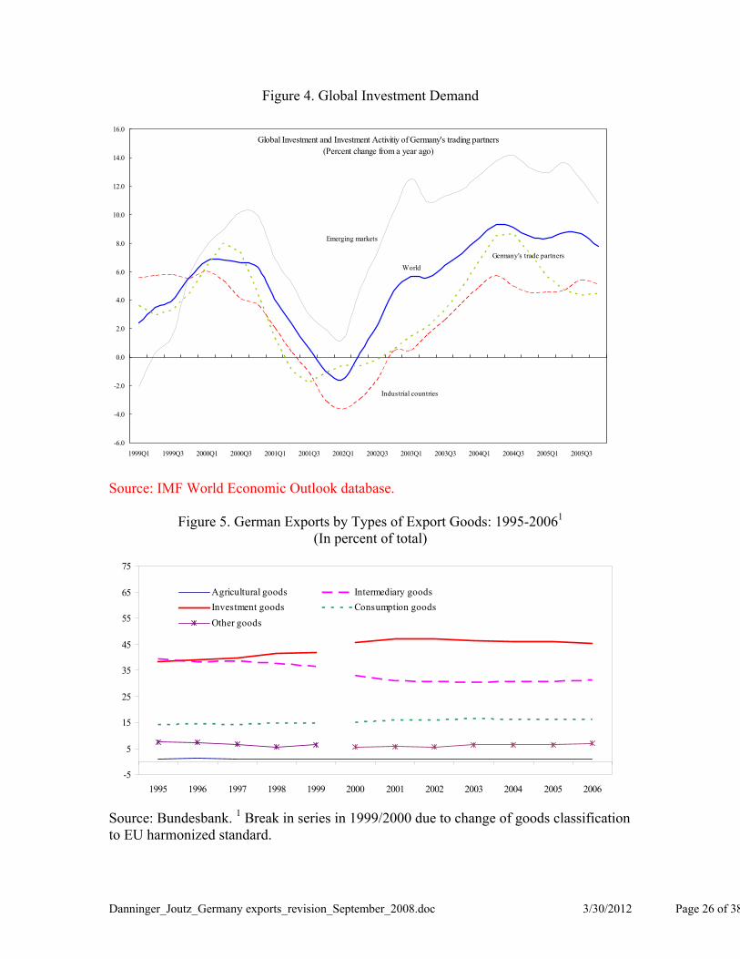
A cursory look at the data suggests that exports in particular of capital goods may have increased. Global growth in traded goods since 2000 was associated by a strong rebound in investment activity especially in emerging markets (Figure 4). This global trend can be compared to investment growth in Germany’s trading partners, assuming that growth of investment activity is linked to a rise of capital goods imports. Investment growth of Germany’s trading partners weighted by export trade shares (Ginv) has been slightly higher than in industrial countries as a whole. A more disaggregated view of German exports by types of export goods offers however no clear evidence: the share of capital goods among overall exports in Germany appears to have been stagnant thus suggesting that there was no faster acceleration in the exports of capital goods compared to other goods (Figure 5). 4. Regionalization of production processes A final explanation is based on increasing the cross-border division of labor to take advantage of lower production costs of labor intensive processes outside Germany. For Germany, this process has been documented by Sinn (2005) and the German Economic Council (2004). Since the mid 1990s, the share of imported inputs in the export sector increased from 28 percent to over 42 percent in 2005 while at the same time domestic value added in the export sector (Ind_VA) decreased from 65 to 56 percent. As an increasing share of industrial production began to be placed abroad, trade volumes increased between German exporters and its subsidiaries or suppliers abroad. To the extent that Germany has taken advantage of this opportunity at a faster pace than other industrial countries, it could have improved productivity and increased its export market share. Several studies have documented the incentives for outsourcing and off-shoring and their effect on trade (Figure 6) Estimates by Marin (2006) on relative unit labor costs in countries outside of Germany indicate large cost savings from relocating production steps. An empirical link between the geographic relocation of production and the trade of goods was also established by a recent Deutsche Bundesbank (2006) study. The empirical evidence supports that increased outbound FDI to new EU member countries from Germany appears complementary to increases in both imports from and exports to these countries.

To conclude, the four presented hypotheses are not necessarily competing explanations. Most likely, all of them have contributed to some degree to Germany’s surge in exports. It is therefore an empirical question to identify their relative contributions. It is also important to note that they have different implications for a continuation of export growth and longer-term economic outlook. Greater cost competitiveness, either through wage moderation or through regionalization of production processes, should have a longer lasting positive effect on export prospects. Also, increasing preferences for German

increased exports of capital intensive goods could therefore be interpreted as a response to a global labor supply shock. Thus, a slowdown in global trade could have a relatively strong negative growth impact on the German economy.


products (Gdem) could signal strength in penetrating growth markets for instance through a desirable product mix. In contrast, if exports were growing primarily because of a first mover advantage or global investment activity, then these developments may come sooner or later to an end, as either the global cycle matures or competitors enter growth markets.

III. DISENTANGLING EXPORT DEMAND

We develop a time series econometric model of German goods exports utilizing information on relative cost competitiveness, export demand, and the structure of production in the export sector. The analysis makes use of integration, cointegration, and error correction in their reduction to the local data generating process and its interpretation. Using quarterly national accounts data beginning in 1993, a baseline and a preferred econometric model are identified using standard inference and estimation methods. We then interpret the parameter estimates and assess whether they are consistent with theory. Robustness tests are carried out to determine the stability of the empirical models. In a final step, we compute the economic impact of the various variables in explaining growth of Germany’s export market share compared to industrial countries from 2000–05. The next part contains a discussion of the data followed by an outline of the empirical modeling strategy. Subsequently we discuss the main findings. 9 While all hypotheses were explored, the discussion focuses on the results from analyzing the regionalization hypothesis, which fit the data the best. The results from the preferred model are used in the final subsection to quantify the contribution of the determinants of export demand. A. Data

The empirical analysis explores the possible cointegrating relationships between five of the variables discussed above: volume of goods export (xgr), the real effective exchange rate based on unit labor costs (REER_u), and global import demand (Gdem), and the share of domestic value added in industry (Ind_VA). The sample period for the analysis is 1993Q1 through 2005Q4. Details on the variables used in the study are presented in Appendix A.

The bulk of Germany’s exports are from the manufacturing sector. The relevant measure for cost competitiveness is hence the real effective exchange rate based on unit labor costs in industry rather than unit labor costs economy wide. The comparison of unit labor costs is quite common and has been applied in a number of recent studies (Deutsche Bundesbank 1998, Hooper 1998).

9 Readers interested in a more technical discussion of the model results can examine Appendix B in the IMF Working Paper version available online at http://www.imf.org/external/pubind.htm.


An increase in REER_u denotes a real appreciation and means a loss of competitiveness. Between 1993 and 1996 cost competitiveness decreased by roughly 30 percent followed by a 25 percent real depreciation thereafter. The real effective exchange rate stabilized in 2001 despite a significant appreciation of the Euro vis-à-vis the US dollar indicating further decreases in relative unit labor costs. To measure global demand, we use a trade weighted index of import volumes by Germany’s trading partners (Gdem) as opposed to sales or manufacturing output. The advantage of this variable is that the estimated elasticity allows inferences about developments of Germany’s market share. A value of 1 indicates a constant market share or that German exports to its trading partners increase proportionately with world trade volume. If the value is less than unity, this indicates a loss in global export market share. Also the results can be more readily compared with other studies.

The global investment activity variable Ginv proxies for the demand for capital goods. The index measures the trade-share weighted investment activity of trading partners and hence, indirectly measures import demand for investment goods. A possible drawback is that this measure overlaps with the import demand measure Gdem.

The share of domestic value added in industry, Ind_VA, attempts to capture the globalization process, in particular the off shoring of production processes. The observed decline in value added in the export sector has been interpreted as a reflection of an increase in the share of imported intermediate goods (Sinn 2006). In the empirical analysis we use value added in industry as a proxy for increased regionalization of production processes.

Data for unified Germany prior to 1993 were either missing or have been dropped due to unification related fluctuations and measurement issue concerns. Table 2 provides summary statistics. Figure 7 shows plots of all variables used in the analysis. Time series plots of the series and their Autocorrelation Function, ACFs, suggested that the series were integrated of order one, which was confirmed through Augmented Dickey Fuller, ADF, tests (Table 2.B).

B. Empirical Modeling Strategy

Specification of the VAR Model

A general to specific approach is employed in estimating the model. First, a simple unrestricted Vector Autoregression, VAR, is estimated and evaluated for statistical fit and stability. Second, the lag structure of the VAR is determined while the evaluation for statistical fit and stability is repeated. Next, we test for equilibrium or cointegrating relation(s) among the variables. Finally, based on the existence of cointegration, we test hypotheses on the relation(s) and interpret the models.

The test for a long-run or equilibrium relationship for German exports demand starts with the estimation of the VAR, which was specified as:


1,1

2,1

3,1

4,1

2 31 2 3

_ _( )

( ) ...

0,

tt t

tt t

tt t t

tt t

pp

t

xgr xgr

REER u REER u ConstantL B

Gdem Gdem Cseasonals

Z Z

where L L L L L

MWN

with L denoting the lag polynomial operator and the individual i terms representing a 5x5 matrix of coefficients at the ith lag. The variable Zt refers to alternative time-varying measures related to the four presented hypotheses. Below we present the results for two models: a baseline model which includes only three variables xgrt, REER_ut, and Gdemt and a final specification related to the fourth hypotheses, which uses Ind_VA as the variable Zt. Alternative models using the variable Ginvt for Zt were explored, but were not supported by the data and are discussed at the end of the results section. Model selection and cointegration analysis All variables were transformed into natural logarithms. Constant and centered seasonal terms are included in each equation, because we use seasonally unadjusted data for German exports. The error terms are assumed to be white noise and can be contemporaneously correlated. Tables 4.A and 4.B contains the finite sample results for lag reduction tests. The test statistic is calculated for maintained models starting with the maximum number of lags, which is equal to five, and then for one fewer number of lags for each time. There are four columns in Table 4A and 4.B with a heading for the maximum number of lags. Below each is the F-test with the p-value reported in brackets for reducing the number of lags to the number in the row. We find that the maximum number of lags is five for the baseline model (Table 4.A) and three lags is appropriate for the alternative model (Table 4.B). Further lags lead to a loss of explanatory power in the respective system. Tables 5.A and 5.B report the results from residual diagnostic tests for the VAR by equation and the vector or system tests. The Portmanteau test and vector tests aimed at detecting autocorrelation, deviation from normality, and heteroskedasticity did not identify significant departures from white noise residuals. To assess robustness, tests for model constancy and structural breaks were conducted using recursive estimation techniques. Changes to the German domestic economy, labor and product market reforms, and the effects of globalization and European integration


could all have impacted the dynamic relationships among the variables and structure. We hence computed two types of recursive Chow tests while taking an agnostic view on the possibility and timing of structural breaks over the period 1993–2005. Results from 1-step Chow and Break Point Chow tests did not reveal any systematic or significant breaks in the estimated VAR model. The test results are graphically presented in Figures 8A and 8B. In a final step, the Johansen procedure is applied to test for the presence of cointegration. The VAR model in levels can be linearly transformed into one in first differences.

1,1 1

2,1 1

3,1 1

4,1 1

_ _ _( )

_ _ _

tt t t

tt t t

tt t t t

tt t t

i

xgr xgr xgr

REER u REER u REER u ConstantL B

Gdem Gdem Gdem Cseasonals

Ind VA Ind VA Ind VA

where

11 2 1

1 2 3

... ,

...

pi i p

p

L

I

Results from Johansen cointegration tests are presented in Tables 6A and 6B; the tables are partitioned into five parts. The first provides the tests for cointegration. The reduced rank standardized coefficients are shown in the second panel. The next two parts show individual hypotheses tests on the and vectors respectively, and the last line reports the joint hypotheses test for the two vectors. Fifth, the final reduced form rank relations are presented.

C. Results

There is evidence of a single cointegrating relation in the two models. Further testing of the and vectors in suggested that the identified relationship can be interpreted as one for export demand. Baseline export demand Results for our baseline model can be found in table 6A. The second panel shows parameter estimates for two vectors under the assumption of a single cointegrating relation. The first standardized eigenvector or vector is normalized on German exports implying that the “long-run” or equilibrium relation explains export demand. We find:

0.17 1.06

(0.11) (0.03)

0.52 (0.18).

t t tExports Real Effective Exchange Rate Global Export Demand

Speed of Adjustment


The coefficients for the real effective exchange rate, LREER_u, foreign demand, and LGdem, are 0.17 and -1.06 respectively.10 The p-value for testing the real exchange rate elasticity is zero is marginal, and cannot be rejected individually. Next, we conduct hypothesis tests on the second vector, which is reported in the third column and shows the speed of adjustment coefficients. If the cointegrating relation we have specified is appropriate, then must be negative for the relation to be consistent with a stationary process. The estimate is -0.52 and significant. We also confirm that the remaining or speeds of adjustment coefficients are sensible. A natural hypothesis at this point is to test whether Germany’s global export market share is stable despite the entry of fast growing emerging markets (e.g. China and India). This hypothesis implies a unit demand elasticity. Imposing this restriction cannot be rejected together with imposing weak exogeneity for the exchange rate and foreign demand (p-value of 0.28). The results for the restricted baseline model are summarized at the bottom of the table where we also report the joint tests for the and coefficients:

0.42 1

(0.10)

0.63 (0.19).

t t tExports Real Effective Exchange Rate Global Export Demand

Speed of Adjustment

The empirical results confirm the basic expectations. Improved cost competitiveness and global growth have the correct signs and the model adjusts fairly rapidly to deviations from the “export fundamentals.” The exchange rate elasticity is about 0.4 percent. Thus a 2.5 percent real appreciation in the Euro will reduce Germany’s goods exports by one percent. These results compare well to estimates by Stahn (2006), which cover a similar time period. However, the price and income measures may be masking the effect of additional information. In particular, there were structural changes in the German economy and export sector. Based on these concerns about omitted variables, we explored alternative models guided by the earlier discussed hypotheses to see whether they offer an improved fit to the data. The preferred export model The share of value added in industry (Ind_VA) improved the model’s explanatory power and addresses these concerns. The preferred specification for the model is reported at the bottom of the table 6B, where we also report the joint tests for the and coefficients. The final cointegrating relationship with weak exogeneity for demand imposed is therefore:

10 The signs are reported as if the sum of the entire vector equals zero, thus opposite to the presentation in a standard export model equation. Standard errors are reported in parentheses.


_ _

0.14 0.78 3.84

0.10 0.08 1.06

: 0.43 , 0.26 , 0.08 .

0.11 0.11 0.03

t t t t

xgr reer u ind va

Exports Real Effective Exchange Rate Global Export Demand Value Added

Speed of Adjustment and

where the standard errors are reported below the coefficients. The empirical results confirm the basic expectations. Improved cost competitiveness, global growth, and value added have the correct signs and the model adjusts fairly rapidly to deviations from the “export fundamentals.” To arrive at this model several diagnostic tests were applied and restrictions tested, the results of which are presented in the upper partitions of Table 6B. The top panel reports the eigenvalues of the Π matrix sorted from largest to smallest. The test for no cointegration (r=0) is rejected at 0.01 with the Trace test (58.17) and at 0.02 with the Max(eigenvalue) test (30.13). There was no evidence suggesting a second cointegrating relation among the variables. The second panel of table 6B reports the initial, unrestricted estimates for two vectors and their associated standard errors assuming a single cointegrating relation. The coefficients for the real effective exchange rate, LREER_u, global demand (LGdem), and the share of domestic value added in industry (Ind_VA) are 0.14, -0.78, and 3.8 respectively. In the third panel we test for the significance of the coefficients individually, jointly and for unit elasticities. All variables have the correct sign and are statistically significant except for LREER_u. A joint test that all three coefficients are zero is rejected with a chi-square statistic of 20.55 and p-value less than one percent. The null hypotheses of unit eleasticities for LGdem and Ind_VA are rejected. The fourth panel of table 6B presents results for tests of the , feedback, coefficients or weak exogeneity tests. The zero restriction for exports, Lxgr, is rejected at one percent consistent with the cointegration and error correction specification. The remaining tests for the individual coefficients are not rejected at five percent. But, the LREER_u and Ind_VA coefficients are rejected at 10 percent. However the joint restriction that they are both zero is rejected at the 5 percent level (the chi-square statistic is 6.44 and has a p-value of 0.04). The weak exogeneity tests suggested that there might be a richer and more complex relationship between the variables explaining export demand. In particular, rather than reducing to a conditional single vector error correction equation, there is evidence that two other variables are influenced by the cointegrating relation. Thus, we reduced the system to a conditional three equation model. We proceeded with joint tests for the and coefficients. The final reduced rank cointegrating relation with weak exogeneity for only LGdem had a chi-square statistic with one degree of


freedom as 0.81 and a p-value of 0.37. Our discussion focuses on the export equation. Further discussion of the other two equations is beyond the scope of this paper. The obtained parameters offered a meaningful economic interpretation. The exchange rate elasticity is 0.14 and indistinguishable from unrestricted baseline export demand model. Thus a seven percent real appreciation in the Euro will decrease Germany’s goods exports by one percent. The global demand elasticity is less than unity about 0.8. Domestic value added has a negative sign meaning that the decline in domestic value added increases export growth. The intuition being that declining value added in industry reflects increased use of imported intermediate inputs and hence improves output and productivity. A decline of domestic value added in industry by one quarter of a percent increases exports by nearly one percent.11 The results above imply that the baseline model suffers from omitted variable bias. We tested whether the information provided by German exporters changing their supply chain process or value added shares improves the statistical fit. When the value added shares are not included, the price elasticity and income elasticity are biased upwards, and overstate their respective impacts on exports, because they ignore the structural changes. Further, our result is consistent with and tends to support Sinn’s efficiency or Bazaar economy argument. However, we cannot determine the degree of the misallocation of inputs, especially capital, and its potential impacts on the economy. In a global marketplace competitive pressures will distribute the content of production to the most cost-efficient producers. The decline of value added is probably driven by larger imported inputs which through volume effects have a positive effect on German net exports. The speed of adjustment coefficient for exports is negative and significant; it has a value of -0.43 implying a fairly rapid correction of a disequilibrium (89 percent after four quarters). If export demand were above the “equilibrium” level last period, this leads to a temporary increase and/or appreciation in LREER_u, the labor cost adjusted effective exchange rate, which is in line with theoretical expectations. In addition it implies there would be a temporary decline in Ind_VA, share of domestic value added in industry. Alternative specifications We explored other modifications to the baseline export demand model by including an indicator of investment demand by Germany’s export partners (LGinv) motivated by the above discussed hypotheses. The Johansen tests for cointegration suggested the possibility of more than one cointegrating relation with the addition of the new variable. We failed to find a second cointegrating relation which was stable or meaningful. Thus,

11 The estimated range at the 95% confidence interval is one half to one and half percent.


we restricted the vector error correction model to a single relation, which however does not deliver economically meaningful results.12 A puzzling aspect of the obtained model was that the coefficients for LGdem and LGinv had opposite signs, while our hypothesis was that both would have the same sign. There are two reasons generating this puzzle, which may also explain why the countervailing influences of the two variables cannot be easily assessed with the current data. First, the result becomes clearer when we compare LGdem and LGinv across different regions. Increases in demand for German goods by other European countries and the US are negatively correlated with investment activity. Since these two regions have large weights in the aggregate investment index for Germany, they may account for the opposite signs. In other words, investment activity and import demand in key partner countries have moved in opposite directions and hence tend to reject the hypothesis that export growth was driven by increased investment activity in partner countries. Second, the investment index may be too crude to pick-up demand for capital goods. The index is based on the assumption that the share of capital goods imports per investment unit is identical across countries. This assumption may be too restrictive. In particular, the import demand for capital goods from fast growing emerging markets may have been underestimated. In light of these considerations we subsequently abandoned this modeling approach. D. Quantifying the contributions to gains in export market share

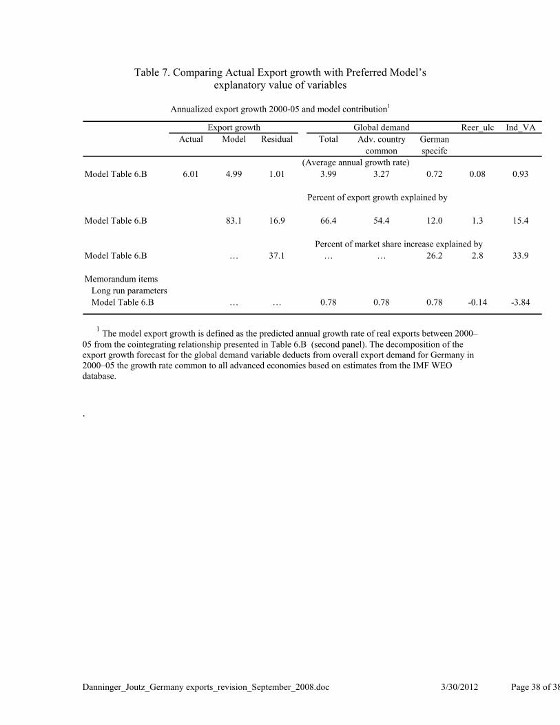
The long-term relationship unearthed in the final model are in a next step used to back out the relative contributions of the different variables to the increase of Germany’s export market share relative to industrial countries. Industrial countries are the natural comparator for Germany and have therefore been chosen as a benchmark. As a starting year we chose the year 2000 when Germany began to increase its export market share. To assess which factors are responsible for the increase in export market share, we first decompose predicted export growth into two components: one is the level of export growth that is necessary to keep the export market share constant vis-à-vis industrial countries; and the remainder that is responsible for changes in the export market share. Before we carry out this decomposition, we must first assess the model fit. If the estimated export models explain only a small fraction of overall export growth between 2000-05, then the decomposition is of limited value. The first line in Table 7 summarizes the model fit and the respective contributions of the individual variables. For the period 2000–05 final model predicts an average annual export growth rate of 5.0 percent. The actual growth rate was slightly higher (6.0) percent indicating that about 80 percent of actual export growth can be explained by the fundamental variables.

12 Results for the alternative specifications are reported in the working paper version: Danninger and Joutz (2007).


The respective model contributions of the variables Gdem, REER_u, and Ind_VA are reported in the columns to the right of the model results. The bulk of export growth, 4.0 percent, is explained by growth in global export demand. An additional 1.0 percent of export growth is explained by the other two variables REER_u (0.08) and Ind_VA (0.93).The bazaar effect appears to explain about 15% of total export growth. We now make a crucial assumption that allows us to assess the relative contribution of the various variables in explaining the increase in export market share compared to industrial countries. We assume that for any industrial country global export demand can be broken into a component common to all industrial countries and a country specific component. The common component captures the demand for exports which keeps market shares unchanged. The country specific part explains changes in market share: a negative specific component would indicate a loss in market share relative to this group, a positive component gains in market share. By implication, the export growth explained by the other two variables (REER_u, Gdem), and the residual (unexplained growth) would also contribute to changes in the export market share. The middle two columns in Table 7 show the decomposition of Germany’s export demand growth into the common and the country specific demand component.13 In both models the bulk of export growth is explained by the common components. From a total of 6.0 percent export growth roughly 3.3 percent (54 percent of model fit) would have been necessary to maintain a constant export market share. The remainder can be attributed to the other variables (0.7 percent from country specific demand, REER_u, Gdem, and Ind_VA), and the rest comes from the residual (1.0 percent). The relative contribution from the four components responsible for the change in export market share is reported in the third panel of Table 7. The German specific component of global demand and the decline in domestic value added account for the bulk of the increase with 26 and 34 percent respectively. Relative cost improvements only account for around 3 percent of the increase in export market share. The unexplained residual component accounts for another 37 percent. The large contribution of the country specific demand is consistent with findings by Everaert, 2005, and confirms that German exporters are benefiting from growth in trading partners. The sizeable contribution of a declining share of Ind_VA lends some empirical support for the Bazaar hypotheses proposed by Sinn (2006). It is also consistent with estimated trade effects of German outward FDI to the new EU member countries (Deutsche Bundesbank 2006) and explains the limited spillovers of export to domestic employment and demand (German Economic Council 2004).

13 Data for export demand for industrial countries comes from the IMF WEO database and reflect trade weighted import demand for these countries. Since Germany is part of this group and its export demand could not be removed from the group average, the estimated of the common component is biased upwards. As a result the country specific export demand component is biased downwards, which underplays its role in explaining the increase in export market share.


The small role of REER_u is surprising at a first glance given prolonged wage moderation. However, the influence of wage moderation on international cost competitiveness appears to be muted by the large effective nominal appreciation of the euro between 2000–05. If this offsetting exchange rate adjustment is taken into account, the small positive contribution of REER_u to gains in export market share is actually quite remarkable. IV. CONCLUSION

Since 2000 Germany’s export market share has gradually recovered. The paper reviews four different hypotheses explaining export growth and evaluates their relative contribution to the gain in export market share. They are: (i) regained cost competitiveness through wage moderation since the mid 1990s; (ii) ties to fast growing trading partners; (iii) increased export demand for capital goods in response to a global increase in investment activity, and (iv) new regionalized production chains in the export sector, for instance, through off-shoring of labor intensive steps. The long-term parameters estimated by the models are consistent with previous empirical findings in the literature. The econometric analysis identifies stable long-run relationships between export growth and variables which measure the proposed hypotheses. The estimates are then used to quantify the relative contribution of these factors to the observed market share increase. The dominant factors explaining the increase in export market share vis-à-vis industrial countries since 2000 are trade relationships with fast growing countries and a suggested trend to regionalized production in the export sector. Together they account for 60 percent of the faster export growth compared to other industrial countries. Improved cost competitiveness played a comparatively smaller role in explaining the brisk export growth. Although the euro experienced a substantial nominal effective appreciation, prolonged efforts in containing costs through wage moderation lowered unit labor costs and neutralized this negative effect. Cost competitiveness improved hence primarily vis-à-vis euro area countries and explains also the significant rise of Germany’s export market share within the eurozone. There was no conclusive evidence of faster export growth due to higher investment expenditures of trading partners and the demand for capital goods. The delayed response of investment activity during the most recent upswing may have not allowed to capture this effect with current data. An important contribution of the paper is its attempt to test whether Germany’s export growth was linked to the emergence of new production chains (Marin 2006). Following a well known literature (e.g. Sinn 2005, 2006) the paper argued that the fall of value added in Germany’s export sector reflects a growing share of traded intermediate inputs in the production process. From this perspective, the empirical link between value added and export growth can be viewed as evidence for a more decentralized production process. This interpretation also helps explain why the recent surge in exports did not translate into a significant employment growth in German industry (Becker et al 2005). While this


finding is intuitively appealing, the empirical evidence is only indirect and further research is needed to confirm this result.


References Becker S. K. Ekholm, R.Jaeckle and M.-A. Muender (2005), Location Choice and

Employment Decisions: A Comparison of German and Swedish Multinationals, Ces-ifo WP 1374, January, Munich.

Blanchard, Olivier J. and Philippon, Thomas (2004), “The Quality of Labor Relations and

Unemployment,” MIT Department of Economics Working Paper No. 04-25. Carlin, W., Andrew Glyn, and John Van Reenan (2001), Export Market Performance of

OECD Countries: An Empirical Examination of the Role of Cost Competitiveness, Economic Journal Vol. 111.

Danninger S. and F. Joutz (2007), What Explains Germany’s Rebounding Export Market

Share? IMF Working Paper 07/24, Washington DC. Davies, Don (1998) Does European Unemployment Prop Up American Wages? National

Markets and Global Trade, American Economic Review 88 478–494. Deutsche Bundesbank (2006) Determinanten der Leistungsbilanzentwicklung in den

mittel- und osteuropäischen EU-Mitgliedsländern und die Rolle deutscher Direktinvestitionen, Monatsbericht Januar 2006, 17–36.

Deutsche Bundesbank (1998), Effects of exchange rates on German foreign trade.

Prospects under the conditions of the European monetary union. Monthly Reports, January 49-58.

ECB (2005), Competitiveness and the Export Performance of the Euro Area, Occasional

Paper Series No 30, June. Everaert L. C Allard, M Catalan, and S. Sgherri (2005), France, Germany, Italy Spain,

Explaining Differences in External Sector Performance among Large Euro Area Countries, IMF Country Report, SM 05/401, Washington DC

German Economic Council (2004) Erfolge im Ausland Herausforderungen im Inland,

Annual Report, (Sachverständigenrat), Wiesbaden. German Economic Council (2000) The Germany Economy in the Autumn 2000,

Economic Bulletin, Vol. 37 No. 11, pp. 345–68, Springer. German Federal Statistical Office (2006) Konjunkturmotor Export, Wiesbaden,

Germany.


Hooper P. and others (1998) Trade elasticities for G-7 countries. Board of Governors of the Federal Reserve System, International Finance Discussion Papers, No 609, April.

Hummels D., Jun Ishii, and Kei-Mu Yi (2001) The nature and growth of vertical

specialization in world trade, Journal of International Economics, Vol. 54, 75–96. IMF (2007) World Economic Outlook: Spillovers and Cycles in the Global Economy,

Washington DC, April. IMF (2004), Germany Staff Report of the 2004 Article IV Consultation, SM 04/134,

Washington DC. Johansen, S. (1988). “Statistical Analysis of Cointegrating Vectors,” Journal of

Economic Dynamics and Control 12, 231-254. Johansen, S. (1991). “Estimation and Hypothesis Testing of Cointegrating Vectors in

Gaussian Vector Autoregressive Models,” Econometrica 59, 1551-80. Kappler, M. and D Radowski (2003). Der Außenhandelskanal. In M. Schröder und P.

Westerheide (eds). Finanzmärkte, Unternehmen und Vertrauen. Neue Wege der internationalen Konjunkturübertragung. ZEW Wirtschaftsanalysen 64, 181–205.

Marin, D. (2006). "A New International Division of Labor in Europe: Outsourcing and

Offshoring to Eastern Europe," Journal of the European Economic Association, MIT Press, vol. 4(2-3), pages 612-622, 04-05.

Meurers, M (2004). Estimating supply and demand functions in international trade: A

multivariate cointegration analysis for Germany. Journal of Economics and Statistics (Jahrbücher für Nationalökonomie und Statistik) 224/5, 530–556.

Milton, A.R. (1999). Erhöhung der Wechselkursreagibilität deutscher Ausfuhren? – Eine

sektorale Analyse. RWI-Mitteilungen 50/4, Oct/Dec, 223–246. Schnatz, B. (2007) Explaining and forecasting euro area exports - which competitiveness

indicator performs best?, ECB Working Paper 877, Frankfurt, Germany. Sinn H. W. (2005) Basar-Ökonomie Deutschland Exportweltmeister oder Schlusslicht,

ifo Schnelldienst 58/6, Munich. Sinn H. W. (2006): The Pathological Export Boom and the Bazaar Effect - How to Solve

the German Puzzle, The World Economy 1157-1175.


Stahn, K (2006) Has the Impact of Key Determinants of German Exports Changes? Results from Estimations of Germany’s Intra euro-area and Extra-euro area Exports, Deutsche Bundesbank, Discussion Paper 07/2006.

Stephan, S. (2002) German Exports to the Euro area, DIW Discussion Paper 286, Berlin. Strauβ H. (2004) Multivariate Cointegration Analysis of Aggregate Exports: Empirical

Evidence for the United States, Canada, and Germany, Kiel Studies No 329, Kiel Institute for World Economics.

Ulman, L., Knut Gerlach, and Paola Giuliano (2005), “Wage Moderation and Rising

Unemployment”. Institute of Industrial Relations. Institute of Industrial Relations Working Paper Series. Paper 110–05.


APPENDIX. VARIABLE DESCRIPTIONS

Sample 1993Q1–2005Q4 xgr

Total goods export volume. Base year 2000, quarterly 1993Q1–2005Q4, billions of Euros. Source: German Federal Statistical Office.

REER_u

Real effective exchange rate based on relative unit labor costs in industry (ULC), Index 2000=100 Source: International Financial Statistics (IFS)

Gdem (Germany’s global export demand)

Export share weighted volumes of real aggregate import volumes (ex/including oil) in Germany’s trading partner countries transformed into an index normalized to 100 = 2000.

Gdemt = i Σi Δmit

i = average 2000–03 share of German goods export to country i. More

precisely: ii

G

x

x where xi are Germany’s exports to country i and xG are

Germany’s total exports. The ratio is averaged over 2000–03.

Δmit = annual growth rate of real goods imports in country i Source: IMF World Economic Outlook database

Ginv (investment activity of German trading partners)

Export share weighted growth volume of real investment activity in Germany’s trading partner countries.

GINVt = i Σi εit invit

εit = national currency/$US exchange rate invit = real volume of investment activity

Source: IMF World Economic Outlook database

Ind_VA (domestic value added in industry) Domestic value added as percent of total output of industrial sector.

Source: German Statistical Office GENESIS database and own calculations


Figure 1. Germany: Export Market Shares in the World and Among Industrial Countries and the Euro Area 1990–2005

Export Market Share Index

Source: ITS1/ Share of German imports in total imports of industrial countries from other industrial countries. 2/ Share of German imports in total imports of euro area from other euro area countries.

60

70

80

90

100

110

120

130

1401

990

199

1

199

2

199

3

199

4

199

5

199

6

199

7

199

8

199

9

200

0

200

1

200

2

200

3

200

4

200

5

200

6

Germany

France

Japan

US

Global index 2000=100

14

15

16

17

18

19

20

21

1990 1993 1996 1999 2002 2005

14

15

16

17

18

19

20

21

Among industrial countries 1/

34

35

36

37

38

39

40

41

42

43

44

1990 1993 1996 1999 2002 2005

34

35

36

37

38

39

40

41

42

43

44

Among euro area 2/

Export Market Share in Percent


Figure 2. Real Effective Exchange Rate at Unit Labor Costs Germany and Euro Area

Real effective exchange rate, index of monthly normalized unit labor costs in manufacturing,

80

85

90

95

100

105

110

115

1990 1991 1992 1993 1994 1995 1996 1997 1998 1999 2000 2001 2003 2004 2005

80

85

90

95

100

105

110

115

120

125

Germany

Euro Area

Source: IMF


Figure 3. World Volume Growth and Germany’s Demand Growth

Global import growth and import growth in German partner countries and industrial countries

-0.05

0.00

0.05

0.10

0.15

1991 1992 1993 1994 1995 1996 1997 1998 1999 2000 2001 2002 2003 2004 2005

Export demand for Germany

Export demand for industrial economies

Global export demand

Source: IMF World Economic Outlook database.


Figure 4. Global Investment Demand

Global Investment and Investment Activitiy of Germany's trading partners (Percent change from a year ago)

World

Industrial countries

Emerging markets

-6.0

-4.0

-2.0

0.0

2.0

4.0

6.0

8.0

10.0

12.0

14.0

16.0

1999Q1 1999Q3 2000Q1 2000Q3 2001Q1 2001Q3 2002Q1 2002Q3 2003Q1 2003Q3 2004Q1 2004Q3 2005Q1 2005Q3

Germany's trade partners

Source: IMF World Economic Outlook database.

Figure 5. German Exports by Types of Export Goods: 1995-20061

(In percent of total)

-5

5

15

25

35

45

55

65

75

1995 1996 1997 1998 1999 2000 2001 2002 2003 2004 2005 2006

Agricultural goods Intermediary goods

Investment goods Consumption goods

Other goods

Source: Bundesbank. 1 Break in series in 1999/2000 due to change of goods classification to EU harmonized standard.


Figure 6. Trends in Offshoring in G7 Countries (In Percent) 1

2

3

4

5

6

7

8

9

1990 1991 1992 1993 1994 1995 1996 1997 1998 1999 2000 2001 2002 2003

United States

United Kingdom

France

Germany

Italy

Source: IMF World Economic Outlook, April 2007, Chapter 5. 1 Offshoring measured as share of imported manufacturing inputs in gross manufacturing output.


Figure 7. Time Series Plot of Main Variable (log levels except for Ind_VA) 1990–2005

1990 1995 2000 2005

4.5

5.0

Lxgr

1990 1995 2000 2005

4.6

4.7

4.8LREERu

1990 1995 2000 2005

4.0

4.5

LGdemo

1990 1995 2000 2005

3

4

5Lginv

1990 1995 2000 2005

0.350

0.375

0.400

ind_va


Figure 8.A Recursive Stability Analysis: Standard Export Demand Model

2000 2005

0.5

1.0

Model 1 5 Lags Recur

1up Lxgr 5%

2000 2005

0.5

1.01up LREERu 5%

2000 2005

1

21up LGdemo 5%

2000 2005

0.5

1.01up CHOWs 5%

2000 2005

0.5

1.0Ndn Lxgr 5%

2000 2005

0.5

1.0Ndn LREERu 5%

2000 2005

0.5

1.0Ndn LGdemo 5%

2000 2005

0.5

1.0Ndn CHOWs 5%

Figure 8.B Recursive Stability Analysis Export Demand Model Driven by Regionalization of Production Processes

2000 2005

0.5

1.0

1.5 1up Lxgr 5%

2000 2005

0.5

1.01up LREERu 5%

2000 2005

1

2

3 1up LGdemo 5%

2000 2005

1

2

3 1up ind_va 5%

2000 2005

0.5

1.0

1.51up CHOWs 5%

2000 2005

0.5

1.0Ndn Lxgr 5%

2000 2005

0.5

1.0Ndn LREERu 5%

2000 2005

0.5

1.0

1.5Ndn LGdemo 5%

2000 2005

0.5

1.0

1.5Ndn ind_va 5%

2000 2005

0.5

1.0Ndn CHOWs 5%


Table 1. Germany: Selected Export Growth Rates and Shares

95-00 00-05 95-05 Share of Exports

2005 (Annual growth rate)

(In percent)

Total exports 9.3 5.6 7.4 100 Of which 1/

European Union … … 7.4 63.3 Euro area … … 6.9 43.3 EU (new) … … 12.5 8.6

Asia 6.2 5.9 6.3 11.0 China 11.4 17.6 14.5 2.7 India -2.3 15.1 6.0 0.5

Oil exporters Saudi Arabia 7.8 8.9 8.3 0.5 Arab Emirates 12.8 14.9 13.8 0.5 Iran 5.4 23.1 13.9 0.5

Source: German Statistical Office. 1/ of which does not add up to total.

Table 2. Summary Statistics 1993Q1–2005Q41

N Means Standard Deviation Lxgr 52 4.8770 0.27603 LREER_u 52 4.6711 0.07372 LGdem 52 4.4651 0.25959 LGinv 52 4.5145 0.14991 Ind_VA 52 0.3603 0.02057 Source: German Statistical Office and IMF World Economic Outlook. 1 Variables in log levels except for Ind_VA.


Table 2.B: Augmented Dickey-Fuller Tests for Unit Roots

Levels - sample 1993q1 2005q4

Variable t-adf beta

Y_lag t-

DY_lagMaximum

Lags AIC

Lxgr 0.025 0.996 n.a. 0 -7.101

LREER_u -2.164 0.878 2.603 2 -7.712

LGdem -1.991 0.966 2.931 5 -11.230

LGinv -2.507 0.944 3.118 3 -10.840

Ind_VA -0.541 0.974 -1.994 3 -9.915

Constant, Trend, and Seasonals Included - Critical Values; 5%=-3.43 1%=-4.01 Constant and Trend Included - Critical Values; 5%=-3.50 1%=-4.14

First Differences - sample 1993q1 2005q4

DLxgr -7.768**-0.122 n.a. 0 -7.116

LREER_u -4.029* 0.267 -2.595 1 -7.655

LGdem -2.801 0.773 -3.669 2 -10.940

LGinv -2.879 0.737 -2.514 2 -10.750

Ind_VA -5.207**-1.686 1.417 4 -9.962

Constant and Seasonals Included - Critical Values; 5%=-2.88 1%=-3.46

Constant; Critical Values; 5%=-2.92%=-3.56 Seasonal Factors included for Lxgr and Ind_VA


Table 3.A: Baseline Export Demand Model: Lag Structure and Reduction Tests, sample 1993Q1–2005Q4

Model T p log-likelihood SC HQ AIC

1 52 48 499.6372 -15.57 -16.68 -17.371

2 52 39 486.0981 -15.733 -16.635 -17.196

3 52 30 474.9738 -15.989 -16.683 -17.114

4 52 21 446.3374 -15.571 -16.057 -16.359

5 52 12 413.0468 -14.975 -15.252 -15.425

Table 3.B: Final Export Demand Model Driven by Regionalization of Production Processes, Model for Lag Structure and Reduction

Tests, sample 1993Q1–2005Q4

Model T p log-likelihood SC HQ AIC

1 52 96 742.8686 -21.277 -23.499 -24.88 2 52 80 716.8998 -21.494 -23.345 -24.496 3 52 64 710.147 -22.45 -23.931 -24.852 4 52 48 670.0764 -22.125 -23.235 -23.926 5 52 32 642.1267 -22.266 -23.006 -23.466


Table 4.A: Baseline Export Demand Model Lag

Structure and Reduction Tests, Sample 1993Q1-2005Q4

Unrestricted Models

Restricted Lags

5 4 3 2

4 2.1975 [0.0303]*

3 2.1396 [0.0096]**

1.9263 [0.0580]

2 3.7668 [0.0000]**

4.1889 [0.0000]**

6.2002 [0.0000]**

1 5.8658 [0.0000]**

6.5102 [0.0000]**

8.3400 [0.0000]**

8.0619 [0.0000]**

Note: F-test of a lag exclusion test with p values in parentheses.

Table 4.B: Final Export Demand Model Driven by Regionalization of Production Processes, Model

Reduction Tests: Lag Length and Specification of the VAR

Unrestricted Models

Restricted Lags

5 4 3 2

4 1.8614 [0.0376]*

3 1.1921 [0.2549]

0.49487 [0.9437]

2 2.1890 [0.0005]**

2.1356 [0.0020]**

4.1603 [0.0000]**

1 2.6454 [0.0000]**

2.6299 [0.0000]**

3.9792 [0.0000]**

2.9962 [0.0004]**

Note: F-test of a lag exclusion test with p values in parentheses.


Table 5.A: Baseline model: Individual Equation and Vector Misspecification Tests for the

Standard Export Demand Model

Lxgr Portmanteau( 6): 3.65372 LREER_u Portmanteau( 6): 1.20985 LGdem Portmanteau( 6): 8.20337 Lxgr AR 1-4 test: F(4,32) 1.7037 [0.1735] LREER_u AR 1-4 test: F(4,32) 0.34946 [0.8424] LGdem AR 1-4 test: F(4,32) 1.3315 [0.2796] Lxgr Normality test: Chi^2(2) 0.83290 [0.6594] LREER_u Normality test: Chi^2(2) 0.75053 [0.6871] LGdem Normality test: Chi^2(2) 2.5739 [0.2761] Lxgr ARCH 1-4 test: F(4,28) 0.41948 [0.7932] LREER_u ARCH 1-4 test: F(4,28) 0.07348 [0.9896] LGdem ARCH 1-4 test: F(4,28) 1.5709 [0.2095] Lxgr hetero test: F(30,5) 0.23698 [0.9949] LREER_u hetero test: F(30,5) 0.27972 [0.9882] LGdem hetero test: F(30,5) 0.16732 [0.9994] Vector Portmanteau( 6): 33.4183 Vector AR 1-4 test: F(36,65) 0.9493 [0.5586] Vector Normality test: Chi^2(6) 3.3193 [0.7678] Vector hetero test: F(180,8) 0.0618 [1.0000]


Table 5.B: Final model: Individual Equation and Vector Misspecification Tests for the Export Demand

Model Driven by Regionalization of Production

Lxgr Portmanteau( 6): 2.82619 LREER_u Portmanteau( 6): 1.00148 LGdem Portmanteau( 6): 7.62194 Ind_VA Portmanteau( 6): 1.37764 Lxgr AR 1-4 test: F(2,34) 0.10128 [0.9812] LREER_u AR 1-4 test: F(2,34) 0.25279 [0.9058] LGdem AR 1-4 test: F(2,34) 4.5998 [0.0048]* Ind_VA AR 1-4 test: F(2,34) 0.15007 [0.9616] Lxgr Normality test: Chi^2(2)0.49661 [0.7801] LREER_u Normality test: Chi^2(2) 5.3022 [0.0706] LGdem Normality test: Chi^2(2)0.12052 [0.9415] Ind_VA Normality test: Chi^2(2) 2.3650 [0.3065] Lxgr ARCH 1-4 test: F(24,11) 0.9640 [0.4426] LREER_u ARCH 1-4 test: F(24,11) 0.2631 [0.8991] LGdem ARCH 1-4 test: F(24,11) 2.035 [0.1166] Ind_VA ARCH 1-4 test: F(24,11) 0.3338 [0.8528] Lxgr hetero test: F(18,17) 0.26675 [0.9967] LREER_u hetero test: F(18,17) 0.64676 [0.8206] LGdem hetero test: F(18,17) 0.62324 [0.8393]

Ind_VA hetero test: F(18,17) 0.50927 [0.9191]

Vector Portmanteau( 6): 67.044

Vector AR 1-4 test: F(64,68) 1.2482 [0.1842]

Vector Normality test: Chi^2(8) 10.620 [0.2242]

Vector hetero test: F(240,43)0.24518 [1.0000]


Table 6.A: Baseline Export Demand Model Cointegration Analysis with Johansen Test: sample 1993Q1–2005Q4

H0:rank eigenvalue loglik for Trace test

[ Prob] Max test [ Prob]

Trace test (T-nm)

Max test (T-nm)

484.3679

0 0.26591 492.405330.54

[0.041]* 16.07

[0.229] 21.73

[0.324] 11.44

[0.614]

1 0.21409 498.668914.46

[0.070] 12.53

[0.092] 10.29

[0.264] 8.91

[0.300]

2 0.036556 499.63721.94

[0.164] 1.94

[0.164] 1.38

[0.240] 1.38

[0.240]

Reduced Rank Standardized Coefficients

Beta Vector Std Err

Alpha Vector Std Err

Lxgr 1 0 -0.51799 0.18397

LREER_u 0.16791 0.11838 0.28222 0.15061

LGdem -1.0584 0.030943 -0.01167 0.02797 Hypotheses Tests for the Beta Vector

LREER_u Zero Chi^2(1) 0.4505 [0.5021] LGdem Zero Chi^2(1) 3.5376 [0.0600] LREER_u and LGdem Zero Chi^2(2) 9.0188 [0.0110]*

LGdem Unit Elastic Chi^2(1) 2.7530 [0.0971]

Hypotheses Tests for the Alpha Vector: Weak Exogeneity

Lxgr Zero Chi^2(1) 3.2877 [0.0698] LREER_u Zero Chi^2(1) 1.7550 [0.1852] LGdem Zero Chi^2(1) 0.0757 [0.7832] LREER_u and LGdem Zero Chi^2(2) 2.6166 [0.2703] Joint Hypothesis Test: W.E and Unit Elasticity

Chi^2(3) 3.8190 [0.2817] Reduced Rank Cointegrating Relation Testing for a Unit Demand Elasticity

Beta Vector Std Err

Alpha Vector Std Err

Lxgr 1 -0.62753 0.19348 LREER_u 0.41898 0.096262

LGdem -1 P-values are in brackets.


Table 6.B: Preferred Export Demand Model Driven by Regionalization of Production

Cointegration Analysis with Johansen Test: sample 1993Q1–2005Q4

H0:rank eigen-value

loglik for Trace test

[ Prob] Max test [ Prob]

Trace test (T-nm)

Max test (T-nm)

681.061 0 0.4398 696.125 58.17 [0.003]**30.13 [0.020]*44.75 [0.094] 23.18 [0.170]1 0.2426 703.348 28.05 [0.080] 14.45 [0.343] 21.57 [0.333] 11.11 [0.645]2 0.1950 708.988 13.60 [0.094] 11.28 [0.142] 10.46 [0.251] 8.68 [0.321]3 0.0436 710.147 2.320 [0.128] 2.320 [0.128] 1.780 [0.182] 1.78 [0.182]

Reduced Rank Standardized Coefficients Beta Vector Std Err Alpha Vector Std Err Lxgr 1 0 -0.3671 0.1199 LREER_u 0.1926 0.1033 0.2050 0.1099 LGdem -0.7707 0.0785 0.0239 0.0239 Ind_VA 4.0097 1.0937 -0.0686 0.0335

Hypotheses Tests for the Beta Vector LREER_u Zero Chi^2(1) 1.8956 [0.1686] LGdem Zero Chi^2(1) 6.0381 [0.0140]* Ind_VA Zero Chi^2(1) 9.0793 [0.0026]** All Three Zero Chi^2(3) 20.553 [0.0001]** LGdem Unit Elastic Chi^2(1) 6.0593 [0.0138]* Ind_VA Unit Elastic Chi^2(1) 5.2927 [0.0214]* LGdem and Ind_VA Unit Elastic Chi^2(2) 6.0684 [0.0481]*

Hypotheses Tests for the Alpha Vector: Weak Exogeneity Lxgr Zero Chi^2(1) 8.8437 [0.0029]** LREER_u Zero Chi^2(1) 3.2272 [0.0724] LGdem Zero Chi^2(1) 0.8122 [0.3675] Ind_VA Zero Chi^2(1) 3.7070 [0.0542] All three Zero Chi^2(3) 11.999 [0.0074]**

Joint Hypothesis Test: W.E and Unit Elasticity for Export Demand and Value Added All three Chi^2(5) 13.755 [0.0172]* Lxgr Chi^2(3) 12.854 [0.0050]** LREER_u Chi^2(3) 9.0895 [0.0281]* LGdem Chi^2(3) 6.4688 [0.0909]

Reduced Rank Cointegrating Relation Testing for a Unit Demand Elasticity Weak Exogeneity of Gdem only

Beta Vector Std Err Alpha Vector Std Err Lxgr 1 -0.4312 0.1119 LREER_u 0.1377 0.1001 0.2585 0.1095 LGdem -0.7836 0.0761 Ind_VA 3.8428 1.0604 -0.0777 0.0343


Table 7. Comparing Actual Export growth with Preferred Model’s explanatory value of variables

Annualized export growth 2000-05 and model contribution1

Reer_ulc Ind_VAActual Model Residual Total

Model Table 6.B 6.01 4.99 1.01 3.99 3.27 0.72 0.08 0.93Model D2 6.01 4.64 1.36 3.95 3.24 0.71 0.11 0.58

Model Table 6.B 83.1 16.9 66.4 54.4 12.0 1.3 15.4Model D2 77.3 22.7 65.8 53.9 11.8 1.8 9.7

Model Table 6.B … 37.1 … … 26.2 2.8 33.9Model D2 … 49.3 … … 25.7 3.9 21.1Memorandum items

Long run parametersModel Table 6.B … … 0.78 0.78 0.78 -0.14 -3.84

Model D2 … … 0.7707 0.7707 0.7707 -0.1926 -0.84

Percent of market share increase explained by

Percent of export growth explained by

Global demandAdv. country

commonGerman specifc

(Average annual growth rate)

Export growth

1 The model export growth is defined as the predicted annual growth rate of real exports between 2000–05 from the cointegrating relationship presented in Table 6.B (second panel). The decomposition of the export growth forecast for the global demand variable deducts from overall export demand for Germany in 2000–05 the growth rate common to all advanced economies based on estimates from the IMF WEO database. .

what explains germany’s rebounding export market share

Documents