Do Hedge Fund Managers Misreport Returns?

Evidence from the Pooled Distribution

Nicolas P.B. Bollen† and Veronika K. Pool

November 19, 2007

†Bollen, nick.bollen@owen.vanderbilt.edu, Owen Graduate School of Management, Vanderbilt University, 401 21st Ave S, Nashville, TN 37240; Pool, vkpool@indiana.edu, Kelley School of Business, Indiana University, 1309 East Tenth Street, Bloomington, IN 47405. The authors thank Cliff Ball, Jim Byrne, Mila Getmansky, Craig Lewis, Bing Liang, Neil Ramsey, Jacob Sagi, Paul Schultz and seminar participants at Georgetown University, Indiana University, the University of Massachusetts, and Vanderbilt University for helpful discussions. Research support was provided by the Financial Markets Research Center.

1

Do Hedge Fund Managers Misreport Returns?

Evidence from the Pooled Distribution

Abstract

We find a significant discontinuity in the pooled distribution of reported hedge fund

returns: the number of small gains far exceeds the number of small losses. The

discontinuity is present in live funds, defunct funds, and funds of all ages, suggesting that

it is not caused by database biases. The discontinuity is absent in the three months

culminating in an audit, funds that invest in liquid assets, and hedge fund risk factors,

suggesting that it is generated neither by the skill of managers to avoid losses nor by

nonlinearities in hedge fund asset returns. A remaining explanation is that hedge fund

managers avoid reporting losses to attract and retain investors.

Hedge funds are currently attracting a great deal of attention from investors,

academics, and regulators for a number of reasons, but primarily due to the returns that

hedge fund managers report. Investors want to share in the riches, academics want to

understand the underlying risk factors, and regulators are concerned about the potential

for fraud. Some members of the SEC support additional regulation of hedge funds, and

championed an amendment to the Investment Advisors Act to force more hedge fund

managers to register.1 Others argue that the low number of hedge fund fraud cases

indicates that there is no need for greater oversight.2 Though the number of fraud cases is

modest, violations of the law may be widespread but undetected. In particular, the

discretion with which managers voluntarily submit returns to databases may permit

purposeful misreporting to attract and retain investors.

1 See the December 2, 3004 Securities and Exchange Commission’s Final Rule Registration Under the Advisers Act of Certain Hedge Fund Advisers, File No. S7-30-04, located at http://www.sec.gov/rules/final/finalarchive/finalarchive2004.shtml. 2 See the dissent of Commissioners Cynthia A. Glassman and Paul S. Atkins to the December 2, 2004 Securities and Exchange Commission’s Final Rule Registration Under the Advisers Act of Certain Hedge Fund Advisers, File No. S7-30-04, located at http://www.sec.gov/rules/final/finalarchive/finalarchive2004.shtml.

2

Hedge fund managers have an incentive to avoid reporting losses. There are at

least two ways this can be accomplished regardless of the fund’s actual performance.

First, as described by Goetzmann et al. (2007), hedge fund fees are accrued monthly but

generally paid annually. Presumably, a manager could turn a loss into a gain by

temporarily returning accrued fees back to the fund. We demonstrate the feasibility of

this mechanism through a simulation exercise later in the paper. Second, and perhaps

more controversially, the manager of a fund that holds illiquid securities can distort

returns by marking up the value of the portfolio. As described by Skeel and Partnoy

(2007), for example, credit sensitive securities such as collateralized debt obligations can

be so complex, and so reliant on subjective inputs, that model values are prone to

manipulation. In addition, Abdulali (2006) explains that managers can distort returns by

opportunistically selecting favorable broker quotes.3

We conduct a simple test for misreporting that measures discontinuities in the

pooled cross-sectional, time series distribution of monthly hedge fund returns. In

particular, we examine the histogram of returns to determine whether certain categories,

e.g. those just below zero, appear systematically underrepresented. Our analytical

framework has been used in prior research linking asymmetric incentives around a fixed

hurdle with breakpoints in the empirical distribution of an outcome. Examples include the

frequency of corporate earnings just below and just above zero (Burgstahler and Dichev

(1997)), the winning percentage of sumo wrestlers in critical bouts (Duggan and Levitt

(2002)), and the ability of management to sponsor shareholder resolutions that receive

just enough votes for approval (Listokin (2007)). Our test is also related to Abdulali’s

(2006) bias ratio, which compares the number of positive returns to the number of

negative returns within one standard deviation of zero.4 An unusually high bias ratio is

suggestive of manipulated returns, although it is unclear what levels are expected under

the null hypothesis of distortion-free returns. In contrast, the null hypothesis for our test is

based on the simple assumption that the distribution of returns is smooth.

3 Reports of this activity also surfaced in the popular press following the 2007 sub-prime mortgage crisis. See “Does it all add up? Worries grow about the true value of repackaged debt” Financial Times (June 28, 2007) page 11. 4 The bias ratio has been implemented in filtering software produced by Riskdata, Inc. to flag suspicious patterns in reported returns.

3

Our test is motivated by the structure of incentive contracts in the hedge fund

industry as well as existing evidence on the interrelation between incentives, fund

performance, and investor capital flow. Outflows lower managerial compensation two

ways. First, a smaller asset base leads to smaller management fees and incentive fees.

Second, satisfying redemptions may require a manager to close losing positions before

arbitrage profits are realized, as in the model of Shleifer and Vishny (1997), resulting in

lower returns and hence lower incentive fees. Consistent with the results of Agarwal et al.

(2007a), we find that annual investor capital flow is positively related to past annual

returns. Furthermore, after controlling for past annual returns, more investor capital is

directed to those funds with fewer reported monthly negative returns. The size of

management and incentive fees, combined with the sensitivity of investor capital flow to

performance, provides a strong motivation to report positive returns.

Evidence that incentives lead to superior returns is reported by Ackermann et al.

(1999), who find that fund Sharpe ratios are positively related to the size of incentive

fees. The authors suggest that the level of incentive stimulates the level of managerial

effort and improved performance as in the model of Starks (1987). Similarly, Agarwal et

al. (2007b) present evidence that fund managers with the greatest incentives, as measured

carefully by the incremental dollar fee per incremental percentage return, report higher

returns. The interpretation in both papers that incentives lead to performance relies on the

assumption that some managers are skillful. The classic method of distinguishing luck

from skill is to measure persistence in performance. Brown et al. (1999) find no evidence

at the annual horizon. Agarwal and Naik (2000) find some evidence at the quarterly

horizon, but not the annual horizon, and explain that the quarterly persistence could be

due to stale valuations. Avramov et al. (2007) show that in a Bayesian setting, and under

certain priors, persistence at the annual horizon can be achieved in portfolios of hedge

funds. The mixed evidence of persistence in performance suggests an alternative

explanation for the link between incentives and subsequent performance: some managers

might distort returns to achieve their goals.

We find that hedge fund returns reported to the CISDM database from 1994 to

2005 have a statistically significant paucity of observations just below zero, and a

statistically significant abundance of observations just above zero. The discontinuity in

4

the distribution is absent on audit dates and the two months leading up to them, and is

also absent in annual returns, suggesting that it is not due to a skillful avoidance of losses.

The discontinuity is also absent in the returns of Commodity Trading Advisors (hereafter

CTAs) and in the returns of factors commonly used to proxy for hedge fund strategies,

suggesting that neither dynamic trading strategies nor non-linearities in underlying asset

returns are the cause. The discontinuity is present in both live and defunct funds, as well

as sub-samples formed by fund age, suggesting that it is not simply a reflection of

survivorship bias or backfill bias. One common attribute of sub-samples that do feature a

discontinuity in the pooled distribution of returns is illiquidity in the funds’ assets. For

example, funds in the top quartile, as ranked by the Getmansky et al. (2004) smoothing

coefficient, exhibit a much larger discontinuity than funds in the bottom quartile.

Similarly, funds in the Distressed Securities category have the discontinuity, whereas

funds in the Equity Market Neutral category do not. This is perhaps no surprise:

distorting returns is more feasible when the opportunity for exerting managerial

discretion is higher.

We make two contributions to the hedge fund literature. First, we implement a

robust, powerful test statistic to prove that the pooled cross-sectional, time series

distribution of hedge fund returns has a discontinuity at zero. Second, we eliminate a

number of possible causes by computing the test statistic on carefully constructed sub-

samples of the data. A remaining explanation is hedge fund managers purposefully avoid

reporting losses. Our results are relevant for the debate regarding the need for hedge fund

regulation. We estimate that approximately 10% of returns in the database we use are

distorted. This suggests that misreporting returns is a widespread phenomenon. Though

small distortions in returns do not directly put a fund’s investors at risk, they may indicate

more serious violations of an adviser’s fiduciary duty. Our results also should give hedge

fund investors a reason to question the accuracy of hedge fund return histories. More

specifically, investors should be cautious when using the number of positive returns as a

metric for fund performance, as this appears to be unreliable.

The rest of this paper is organized as follows. Section I relates our study of hedge

fund returns to existing studies of discontinuous distributions and hedge fund anomalies.

Section II discusses alternative explanations for the discontinuity in hedge fund returns

5

and how we test them. Section III describes the data and Section IV describes the

empirical methods employed in the analysis. Section V presents our results. A brief

summary is provided in Section VI.

I. Related Literature

Discontinuities in distributions have recently been used as a forensic tool in at

least two other contexts: corporate earnings management and corruption in the sports of

sumo wrestling and NCAA basketball. These disparate topics share a feature that leads to

discontinuities in distributions: highly asymmetric incentives around a fixed hurdle. For

earnings management, the hurdle is zero in the level or change in earnings; for sumo

wrestling, the hurdle is a winning record within a tournament; and for NCAA basketball,

the hurdle is the “spread” in betting lines. In all cases, academic studies compare the

frequency of outcomes on either side of the discontinuity to provide evidence that the

asymmetric incentives affect behavior. In order to separate innocuous explanations, such

as increased effort, from an explanation based on fraud, researchers employ various

context-specific tests.

Duggan and Levitt (2002) present evidence of corruption in elite Japanese sumo

wrestling tournaments. They explain that in these tournaments, each wrestler participates

in 15 bouts. Wrestlers with eight wins or more are said to achieve “kachi-koshi” and

advance in official rankings, while those with losing records fall. More importantly, the

eighth victory leads to the largest incremental change in ranking, resulting in bouts in

which bribing can be mutually beneficial. Consider, for example, two wrestlers heading

into the 15th bout, one with seven wins and seven losses, the other with eight wins and six

losses. The former wrester has much more to gain by winning the last bout than the latter

has by losing, and they could enter into an agreement in which the former wrestler wins,

perhaps with the understanding that the latter wrestler will win the next time they meet.

Duggan and Levitt find that in their sample of 60,000 wrestler-tournament observations,

12.2% of wrestlers finish the tournament with seven wins and 26.0% finish with eight

wins. Both are statistically significantly different from the expected frequency of 19.6%,

under the assumption that all wrestlers are identical and bouts are independent. To

6

distinguish between increased effort and match rigging, the authors examine the

frequency with which wrestlers who win their eighth bout also win the next time they

face the same opponent, and find that it is abnormally low, suggesting a quid pro quo. In

subsequent meetings, the frequency returns to its unconditional mean.

Wolfers (2006) points out that the structure of bets on college basketball in the

U.S. generates asymmetric payoffs involving the winning margin of favored teams.

Bettors wager whether a favored team will win by at least as much as a quoted amount

known as the spread. Players on heavily favored teams are concerned primarily about

winning, rather than beating the spread, hence a bettor and players on a heavily favored

team could enter into a mutually beneficial agreement. The bettor could bribe the players

to shave points so that the winning margin is less than the spread, but the players could

still win the game. In a sample of 44,120 games, Wolfers finds that teams favored by less

than 12 points win but do not cover the spread 40.7% of the time, whereas teams favored

by at least 12 points win but do not cover the spread 46.2% of the time. This evidence

suggests that heavily favored teams sometimes purposely cap the winning margin so that

it is less than the spread.5

In the accounting literature on corporate earnings, several studies have

documented evidence of a discontinuity in earnings or changes in earnings around zero.

Hayn (1995), using data from 1963 to 1990, finds a discontinuity in the pooled cross-

section, time series distribution of earnings: the mass with just-positive earnings is

significantly greater than the mass with just-negative earnings. She argues that this

implies earnings are managed to avoid losses. Burgstahler and Dichev (1997), using data

from 1976 to 1994, find similar results for changes in earnings. They argue that top

management faces strong incentives to avoid reporting earnings decreases, citing

evidence that firms with a consistent pattern of earnings increases feature higher price to

earnings ratios than other firms with comparable earnings.

5 Bernhardt and Heston (2006) argue that the results can be explained by normal game management behavior by heavily favored teams, e.g. perhaps heavily favored teams avoid scoring excessively at the end of games as an act of good sportsmanship.

7

Our study is related to those in sports corruption and earnings management in the

sense that hedge fund managers may perceive an asymmetric response to reported returns

around zero. Anecdotal evidence suggests that a zero return is a powerful quantitative

anchor. Waring and Siegel (2006), for example, argue that many institutional investors

pursue “absolute return” strategies based partly on the desire to consistently achieve

positive returns in any market environment. Also, the “cockroach theory” implies that

investors will overreact to the slightest bit of bad news, such as a negative monthly hedge

fund return, because they fear that more bad news lurks. We test this conjecture by

regressing annual investor capital flow on lagged annual returns and the number of

months in the prior year with positive returns, as in Agarwal et al. (2007a). The

coefficient on the latter variable is positive and significant, both statistically and

economically. Hence we compare the mass of observations with just-positive returns to

those with just-negative returns, in exactly the same spirit as Hayn (1995) and

Burgstahler and Dichev (1997).

Several existing studies in fund management examine related phenomena. Asness

et al. (2001) find that the correlation between hedge fund returns and lagged S&P 500

returns is larger when hedge fund returns are low, suggesting that some managers

understate poor performance. Getmansky et al. (2004) show that if a manager

purposefully smoothes returns, the fund’s volatility will be biased downwards, the fund’s

Sharpe ratio will be biased upwards, and fund returns will be serially correlated. Serial

correlation is only indicative of misreporting, however, as it can also be the result of

innocuous marking to model when funds are invested in illiquid securities. Bollen and

Pool (2006) conjecture that a manager would be more likely to smooth losses than gains,

resulting in greater serial correlation when funds perform poorly. Cross-sectional analysis

indicates that the propensity for funds to feature asymmetric serial correlation is

positively related to proxies for the risk of capital flight. Goetzmann et al. (2007) study

how managers can manipulate performance measures through information-less trading

strategies. Our focus on loss-avoidance is related in the sense that the number of losses is

a form of performance measurement. However we conjecture that the loss-avoidance may

be accomplished via distortions in valuation or expense accounting, whereas Goetzmann

et al. study manipulation via trading strategies.

8

Two other papers are especially relevant. Carhart et al. (2002) study the daily

returns of equity mutual funds around quarter-ends and year-ends. They find that funds

with the highest year-to-date returns tend to feature larger returns on the last day of a

quarter or a year, and that these returns are largely reversed the following day. They

present evidence that some mutual fund managers temporarily inflate the value of fund

assets by adding to their positions of illiquid stocks on the last day of a quarter or a year.

Buying pressure increases the trade prices, and the entire position can be revalued

upwards. Similarly, Agarwal et al. (2007a) find that average hedge fund returns are

higher in December than all other months. They measure the incentive for a particular

fund manager as the “delta” of his compensation contract, and find that the December

pattern is more pronounced for those managers with higher incentives.

The phenomenon we document differs from the calendar-related patterns in

Carhart et al. (2002) and Agarwal et al. (2007a) in at least two important ways. First,

while the other studies are interested primarily in year-end returns, we study the

avoidance of negative returns at all points throughout the year. To the extent that fund

managers use the history of their reported returns as a means of advertising their funds,

they would be concerned with returns that stand out as being particularly poor regardless

of when they occur during the year. Second, and perhaps more important, while Carhart

et al. (2002) and Agarwal et al. (2007a) focus on the mean of the distribution of returns,

we study the shape of the entire distribution. Of particular interest is the frequency of

returns around zero. Thus, our analysis does not rely on a factor model to compute

abnormal returns. This is important because the existing literature has not come to

consensus on appropriate risk adjustments. Work by Fung and Hsieh (2004), Mitchell and

Pulvino (2001), and Agarwal and Naik (2004) all offer different risk factors that may or

may not be relevant for a given individual fund. Furthermore, Bollen and Whaley (2007)

argue that even after allowing factor exposures to vary though time, the typical individual

hedge fund has adjusted R-squared far below 50%, so that abnormal returns may reflect

unspecified sources of risk.

9

II. Alternative Explanations

A number of alternative explanations for any discontinuity in the distribution of

hedge fund returns would eliminate the implication that some hedge fund managers

distort their reported performance. In this section, we describe three alternatives based on

managerial skill, the distribution of underlying asset returns, and well-known database

biases. We also explain how we will distinguish these alternatives from an explanation

based on purposeful misreporting.

A. Skill

Perhaps some hedge fund managers skillfully avoid losses through dynamic

trading or security selection. If so, then we should see no difference between the

distribution of returns around audits and the distribution during other months, since there

is no reason to expect a fund manager’s ability to avoid losses to diminish on or near

audit dates. If, however, the discontinuity is due to distortions, their prevalence may be

reduced when the lens of an auditor is placed on the fund. Liang (2003) asks what impact

auditing has on the reporting behavior of hedge fund managers; his prior is that audited

funds feature more accurate returns. He compares audited to non-audited funds several

ways. He finds 36 pairs of on-shore and off-shore funds that are otherwise equivalent.

The 20 non-audited pairs have return discrepancies that are twice as large in absolute

value as the 16 audited pairs of funds. He also examines returns using two versions of the

TASS database, one from July 31, 1999 the other from March 31, 2001. He finds 3,638

discrepancies. On average, those from non-audited funds are one-third larger in absolute

value than those from audited funds.

Another way to test the skill-based explanation is to compare the distributions

based on annual returns to the distributions of monthly returns. Skillful managers would

be able to continually avoid losses; hence we would expect to see a discontinuity in the

distribution of annual returns if this explanation is true. However, if the loss-avoidance

occurs via distortions, then the discontinuity would not be observed at the annual

frequency. A manager who rounds up returns in some months must reverse the

overstatement, or else the fund’s reported net asset value would drift away from true

10

value. Similarly, a manager who returns fees to boost returns in some months must

expense them by the end of the year to receive appropriate compensation.

B. Non-linearities in underlying assets and strategies

The dynamic strategies employed by some hedge fund managers may result in a

relative paucity of return observations just below zero. Similarly, if some hedge fund

portfolios contain securities with option-like payoffs, then perhaps we would see a

discontinuity in the pooled distribution of reported returns. We address this explanation

two ways.

First, we compare the pooled distribution of reported returns from hedge funds to

the pooled distribution of reported returns from CTAs. Managers in both classes of funds

are free to use dynamic strategies; hence we might expect to observe the same kind of

discontinuity in both distributions. If, however, the kink is due to distortions in reported

returns, then we might expect to see a less significant discontinuity in the CTAs. The

reason is that CTA managers primarily invest in highly liquid futures contracts; hence

distorting reported returns would be more difficult.

Second, we examine the distribution of asset based style factors that mimic some

of the dynamic strategies employed by some fund managers, and are constructed directly

from market prices of underlying assets. These distributions are therefore free of

distortions. If the strategies inherently feature discontinuous distributions, then these asset

based style factors should feature distributions similar to those of the hedge funds. To

make the comparison meaningful, we regress each hedge fund’s return series on a set of

commonly used style factors. Then we construct a fitted return based on the estimated

factor loadings and corresponding factor returns. This allows exposures to vary across

factors and across funds.

C. Database biases

The well-known survivorship bias described in Brown et al. (1999) may result in

a distribution featuring fewer observations of poor returns than expected, even if the

11

reported returns are accurate. Ackermann et al. (1999) argue that both superior

performers and inferior performers may stop reporting, and present evidence that these

groups somewhat offset each other in the pooled distribution of returns. Ackermann et al.

also discuss back-fill bias, in which only successful funds initiate reporting to a database

and report superior historical returns. While both survivorship bias and back-fill bias

might result in fewer observations of poor returns than expected, they do not necessarily

imply a discrete break in the distribution at zero, but rather a shift in location of the entire

distribution. Nevertheless, we test for the possible impact of survivorship bias and back-

fill bias by first discarding the first 12 months of observations, eliminating the impact of

back-fill, and then searching for a discontinuity in live funds and defunct funds

separately. In addition, we examine the distribution of returns for funds at different stages

in their reporting history. We pool observations during the nth year in funds’ lives. This

allows us to investigate whether the discontinuity is only present during the beginning of

a fund’s reporting history, consistent with back-fill bias, or more prevalent during later

years in a fund’s reporting history, consistent with survivorship bias. If, however, the

discontinuity is present in all sub-samples stratified by fund age, then managerial

distortion appears to be a more likely explanation.

III. Data

The hedge fund data used in our empirical analysis are from the Center for

International Securities and Derivatives Markets (CISDM) database. The sample period

is from January 1994 through December 2005. The CISDM database includes live and

defunct hedge funds, funds of funds, CTAs, commodity pool operators, and indices. We

focus attention on the return of hedge funds since the return of a fund of funds reflects the

behavior of a number of individual hedge fund managers as well as the fund of funds

manager.

We eliminate all observations of 0.0000 and consecutive observations of 0.0001.

On the one hand, these observations may represent missing data (i.e., the fund fails to

report in the given month), while on the other, they may reflect fund managers’ attempt

to avoid reporting negative returns. To be conservative, we apply the following filters.

12

First, we eliminate returns that are exactly zero from each time series. In addition to

missing observations, zeros may reveal conservative managers’ choice not to change

portfolio values, when no reliable market price is available. Second, we consider two or

more consecutive observations of 0.0001 to be missing observations, and delete these

from funds’ return histories. After applying these exclusionary criteria, 215,930 hedge

fund return observations from 4,286 unique funds and 64,562 CTA return observations

remain in our sample.

As described in Section II, in part of our analysis we estimate linear factor models

for hedge fund returns. We collect a set of ten factors that are used in the existing hedge

fund literature to proxy for the trading strategies employed by hedge fund managers.

These factors are drawn from three sources. The three Fama-French factors, the excess

return of the market and the returns of size and value portfolios, are from Kenneth

French’s website. Five trend-following factors, which are the returns of portfolios of

options on bonds, foreign currencies, commodities, short-term interest rates, and stock

indexes, are obtained from David Hsieh’s website. The change in the yield of a ten-year

Treasury note and the change in the credit spread, i.e. the yield on ten-year BAA

corporate bonds less the yield of a ten-year Treasury note, are obtained from the U.S.

Federal Reserve’s website. To estimate the factor model, we also require a risk-free rate,

and for this we use the one month T-Bill rate from Kenneth French’s website.

For robustness, we test for a discontinuity in the distribution of stock returns and

equity mutual funds from 1994 through 2005. We use NYSE/AMEX and NASDAQ

monthly stock returns from CRSP, eliminating those that are exactly zero, and CRSP

mutual funds from 1994 through 2005, with ICDI objective codes AG, GI, and LG and

all domestic equity Standard & Poor’s style codes.

IV. Empirical Methodology

Our empirical methodology uses histograms of hedge fund returns to test whether

the underlying densities possess significant discontinuities. Subsection A reviews optimal

histograms, and describes the binomial tests for discontinuity used in existing literature.

Subsection B introduces our discontinuity test that uses a smooth kernel density estimate

13

to establish a more flexible null hypothesis. Subsection C shows results when our test is

applied to individual stock returns and mutual funds. Since these asset classes are free of

the distortions studied in the paper, these results can be interpreted as determining

whether our test is prone to false positives.

A. Histograms

The most important parameter that determines the statistical properties of a

histogram, as a density estimator of some underlying true distribution, is the bin width, b.

When the bin is too small, the histogram appears jagged; in our context, sampling

variability will cause the histogram to feature discontinuities when none exist in the

underlying distribution. When the bin is too large, the histogram may appear continuous,

even if the true distribution features discontinuities.

Several criteria exist for determining the optimal bin width. For instance, one may

choose a bin that minimizes the mean squared error (MSE):

(1) ( ) ( ) ( ) ( ) ( )( )22ˆ ˆ ˆMSE E ; variance ; bias ;t f t b f t f t b f t b⎡ ⎤ ⎡ ⎤ ⎡ ⎤= − = +⎣ ⎦ ⎣ ⎦ ⎣ ⎦ ,

where ( )f t is the true density at point t, and ( )ˆ ;f t b is an estimator of the true density

based on the chosen bin width. The breakdown in (1) clearly illustrates the tradeoff

between the variance and bias of the estimator. Increasing the bin width decreases the

variance of the estimator, but increases the bias, and vice versa. An optimal bin choice is

one that balances the variance and the bias. Other criteria include the integrated squared

error, the mean integrated squared error, or the integrated absolute error. See Pagan and

Ullah (1999) for further discussion.6 The resultant optimal bin with is a function of the

sample size and a measure of dispersion. Scott (1979) suggests the sample standard

deviation as a measure of dispersion, whereas Freedman and Diaconis (1981) use the

interquartile range. Silverman (1986) argues that using the smaller of the two results in a

6 Different criteria result in different statistical properties and different rates at which the density estimator converges to the true underlying distribution. In practical applications, the most popular choices are derived by Scott (1979), Freedman and Diaconis (1981), and Silverman (1986).

14

more robust estimator. In selecting the optimal bin width, we choose to minimize the

MSE and use Silverman’s approach to estimate dispersion. More specifically we set bin

width b equal to:

(2) 151.364 min ,

1.340Q nα σ

−⎛ ⎞× ⎜ ⎟⎝ ⎠

where σ is the empirical distribution’s standard deviation, Q is its interquartile range, n is

the number of observations, and α is a scalar that depends on the type of underlying

distribution assumed. Devroye (1997) shows through simulation that the definition in (2)

is robust to alternative distributional assumptions. To proceed, we set 0.776α = ,

corresponding to a normal distribution.

Figure 1 illustrates the impact of bin width by plotting the histogram of the full

sample of hedge fund returns using three different bin widths. The three figures cover

slightly different ranges due to the different bin widths, but all run from approximately

negative 5% to positive 5%. Figure 1A uses the optimal bin width of 19 basis points.

Bold bars indicate bins bracketing zero. Figure 1B uses a bin width of 10 basis points,

resulting in an erratic pattern for positive returns. In contrast, Figure 1C uses a bin width

of 57 basis points, and much of the general shape of the distribution is lost.

While the histogram provides a visual evaluation of our hypothesis, the next step

is to develop an objective, quantitative evaluation that will allow us to test the statistical

significance of a discontinuity in the distribution. Let N be the number of bins in a

histogram, with labels 1 though N from left to right. Suppose we are interested in

determining whether there is a discontinuity in bin i. Two approaches exist in the

earnings management literature; both assume that changes in the height of the histogram

across bins to the left of bin i should be comparable to changes to the right of bin i.

Burgstahler and Dichev (1997) test whether the number of observations in bin i is

significantly different from the average number of observations in the two immediately

adjacent bins 1i − and 1i + . Degeorge, Patel, and Zeckhauser (1999) test whether the

height of bin i (measured as a percentage of all observations) is significantly different

than the average of the ten bins surrounding it, taking into account the sample standard

deviation of bin heights in this neighborhood. While these approaches are appealing in

15

that they are related to the idea of taking numerical derivatives, they use only a small

subset of the data to evaluate their test statistics, and make a potentially restrictive

assumption regarding the shape of the underlying density under the null hypothesis, i.e.

that it is approximately linear in the neighborhood of the bin in question. This assumption

could lead to false rejections of the null hypothesis when the underlying density has

significant curvature. Further, and perhaps more important, every bin that has too many

or too few observations confounds the analysis of adjacent bins, which again could lead

to false rejections of the null. To address these potential size issues, we propose a new

approach that uses every observation to estimate a flexible smooth density, fitted to the

data, to establish the null hypothesis.

B. Our approach

The first step in our test design is to identify a smooth distribution that captures

the salient features of the empirical distribution, save for any discontinuities in the

density function. The smooth distribution serves as a reference, and we use it to estimate

the expected number of observations in each bin of the histogram, and the corresponding

standard deviation, under the null hypothesis that no discontinuity exists. It is crucial in

our approach that the reference distribution fits the empirical distribution well. While this

is difficult to achieve with a parametric distribution, we fit nonparametric kernel densities

using a Gaussian kernel. The resulting density estimate at a point t is defined as:

(3) 1

1ˆ ( ; )n

i

i

x tf t hnh h

φ=

−⎛ ⎞= ⎜ ⎟⎝ ⎠

∑

where h is the bandwidth of the kernel, n is the number of observations, x is the data, and

φ is the standard normal density. The choice of bandwidth is driven by the same tradeoff

between the variance and bias of the estimated density that is described above for the bin

width of a histogram. Since we use the Gaussian kernel to construct the reference

distribution, and we assume the underlying distribution is Gaussian when choosing the

optimal bin width, the optimal bandwidth is identical to the optimal bin width.

16

The second step in our test design uses an estimate of sampling variation in the

histogram to determine whether the actual number of observations in a given bin is

significantly different than expected under the null hypothesis of a smooth underlying

distribution. We estimate sampling variation two ways.

First, we integrate the kernel density along the boundary of each bin to compute

the probability that an observation will reside in it. Let p denote this probability and n the

number of observations in a sample. The Demoivre-Laplace theorem states that the actual

number of observations that will reside in the bin is asymptotically normally distributed

with mean np and standard deviation ( )1np p− . At a 5% significance level, for

example, we would reject the null hypothesis that the true probability is p if the actual

number of observations in the bin is below ( )1.96 1np np p− − or above

( )1.96 1np np p+ − .

Second, for robustness, we generate random samples from the fitted kernel

density, construct corresponding histograms, and then determine the range of bin heights

to establish the cutoff levels for rejecting the null hypothesis. We adopt the algorithm

summarized in Hörmann and Leydold (2000). The algorithm draws from the original

sample with replacement and adds noise to the resampled data. The noise component is

drawn from the kernel, and its variance is scaled by the corresponding optimal

bandwidth. This smoothed bootstrap creates random variates that are centered around

sample datapoints hence mimicking the idea of the kernel density method. See the

appendix for details. We generate 1,000 simulated samples in this manner, each of length

equal to the actual sample. For each of the simulated samples, we record the number of

observations that fall in each bin, and then compute the average and standard deviation

across the simulations. These are then used to construct critical values as described

above. In all cases, the two approaches result in critical values that are extremely similar

and provide qualitatively identical inference.

To illustrate, Figure 2 displays a histogram using the full sample of 215,930

monthly hedge fund returns. The optimal bin width is 19 basis points. The tails are not

displayed to focus attention on the discontinuity near zero. The two solid black vertical

17

bars highlight the frequency of observing returns in the bins above and below zero: the

discontinuity is clear. Three curves are plotted which indicate the frequency of observing

returns in each bin according to the kernel estimate of the underlying density, as well as

the upper and lower 99% confidence bands generated from 1,000 simulations. The two

bins that bracket zero breach the confidence bands by a wide margin.

To compare the small sample properties of our test to the Burgstahler and Dichev

(1997) approach, we conduct a simulation exercise. Each simulation begins with 10,000

draws from a normal distribution with mean 1% and standard deviation 3%,

approximately equal to the sample moments of the hedge fund returns in our sample. A

histogram is constructed with optimal bin width of 50 basis points. Then, 15% of the

observations in the bin directly to the left of zero are displaced and added to the bin

directly to the right of zero. We then execute both the Burgstahler and Dichev test, and

our test based on the kernel density estimate, on each bin. We repeat for a total of 1,000

simulations. Figure 3A shows the percentage of the simulations for which the Burgstahler

and Dichev test rejects the null hypothesis for the 10 bins centered on zero. The power of

the test for the affected bins is close to 100%. However, over 40% of the simulations

reject the null because the second bin to the left of zero appears to have too many

observations relative to the bin from which observations were displaced, and over 20% of

the simulations reject the null because the second bin to the right of zero appears to have

too few observations relative to the bin to which observations were moved. Figure 3B

shows the results for our test. The power is comparable at the two affected bins, and the

other bins show far fewer rejections than in Figure 3A. This result indicates that our test

has better small sample properties.7

C. Stocks and mutual funds

Before turning to our analysis of hedge fund returns, we apply the statistical test

for a discontinuity on samples of individual stock returns and equity mutual fund returns.

In neither case is there room for distortion: stock returns are based on trade prices and 7 For robustness, we also compute the Burgstahler and Dichev (1997) test statistic in each analysis. Though it differs in magnitude from ours, the two tests reject the null hypothesis on the same subsets of the data.

18

mutual fund returns are computed from net asset values that are confirmed daily by

custodians.

The distribution of stock returns may be affected by microstructure effects. For

this reason, Figure 4 shows results for stocks over three sub-periods defined by tick size:

January 1995 through May 1997 (eighths), July 1997 through August 2000 (sixteenths),

and April 2001 through December 2005 (decimals). The two gaps between the three sub-

periods are excluded to avoid mixing data from different regimes. In both the NASDAQ

and NYSE/AMEX samples, the frequency of observing returns in the two bins around

zero is significantly lower than surrounding bins. This is likely due to trades occurring at

the bid price on the beginning or ending of the month and the ask price on the other date.

Indeed, as the tick size shrinks, and bid-ask spreads narrow, the discontinuity in the

distribution becomes insignificant.

Managers of U.S. equity mutual funds have little opportunity to distort returns

through misreporting or creative expense accounting given the oversight required by the

SEC’s Investment Company Act. As mentioned in Section I, however, Carhart et al.

(2002) present evidence that trading in illiquid stocks can temporarily boost returns. This

distortion is reversed quickly, and likely occurs only at the end of a quarter; hence we

would not expect to observe a discontinuity at zero in the pooled distribution of mutual

fund returns. Figure 5 shows histograms for the 12 years 1994 through 2005 separately.

The shape of the histogram varies through time. In only three of the 12 years (1994,

2003, and 2004) is the number of returns in the bin just below zero less than expected at

the 5% level, and in 2002 the bin is significantly larger than expected. In seven of the

years, there are bins with negative returns and with greater mass than the bin just below

zero, indicating that negative returns are not systematically being shifted to the right of

zero. These results suggest that the discontinuity at zero is neither a robust nor an

important feature of mutual fund returns.

V. Results

The top graph of Figure 6 reproduces the histogram in Figure 2 but includes the

tails as well. Two features are readily apparent. First, as noted before, there appears to be

19

a sharp discontinuity in the distribution at zero. This is objectively corroborated by the

bottom graph, which plots the value of the test statistic measuring whether the height of a

vertical bar is different than expected given the smoothed kernel estimate of the

underlying distribution. The frequency of returns just below zero is significantly lower

than expected, whereas the frequency of returns above zero is significantly higher than

expected, in both cases the test statistics are far in excess of the 99% confidence bands.

Second, the entire distribution to the left of zero appears deflated relative to the

corresponding mass to the right of zero. Table 1 lists the value of the test statistics for the

two bins bracketing zero when the discontinuity is measured on yearly sub-samples of the

data. In all years, the bin below zero is statistically significantly underrepresented in the

annual distributions. And in all years except 1996, the bin above zero is statistically

significantly overrepresented. Thus the discontinuity is a pervasive phenomenon in the

pooled distribution of hedge fund returns. An obvious explanation for these results is that

some hedge fund managers purposely avoid reporting losses. Before jumping to that

conclusion, however, we examine their motivation for doing so, as well as a battery of

alternative explanations.

A. Flow-performance

One reason why managers might avoid reporting losses at the monthly frequency

is if investors are more likely to invest in hedge funds with a higher percentage of

positive returns. Prior studies report strong evidence of a relation between mutual fund

performance and the subsequent flow of investor capital into or out of a fund. See, for

example, Chevalier and Ellison (1997), Sirri and Tufano (1998), Busse (2001), and Del

Guercio and Tkac (2002). Brav and Heaton (2002) argue that if a relevant feature of the

economy is unobservable, e.g. managerial ability, then the flow-performance relation can

be interpreted as the result of rational learning. Ippolito (1992), Lynch and Musto (2003),

and Berk and Green (2004), among others, interpret the flow-performance relation as a

reflection of investors updating their beliefs about managerial ability and expected

mutual fund returns. Agarwal et al. (2007a) study the flow-performance relation in hedge

funds, and find that the fraction of prior months in which a fund delivered positive returns

20

adds incremental explanatory power in a regression of fund flow on lagged returns. This

result motivates our focus on a kink in the distribution of reported returns at zero.

To examine the relation between fund flow and reported losses, we run the

following regression:

(4) ( ) ( ), 1 2 , 1 1 2 , 1 , 1 3 4 , 1 , 1 ,i t i t i t i t i t i t i tF Y Y R Y NPOSα α β β β β ε− − − − −= + + + + + +

where ,i tF is the percentage fund flow for fund i in year t, , 1i tY − is an indicator variable

that equals 1 if fund i was age 3 years or less in year 1t − and 0 otherwise, , 1i tR − is

cumulative annual return, and , 1i tNPOS − is the number of months with positive returns.

As is standard in the flow-performance literature, we estimate fund flow from the

difference in successive observations of total net assets, adjusted for returns, as follows:

(5) ( ), , 1 ,

,, 1

1i t i t i ti t

i t

TNA TNA RF

TNA−

−

− +=

The computation in (5) assumes that fund flow occurs at the end of the year. For

robustness, we also construct fund flow under the assumption that all activity occurs at

the beginning of the year. Results are qualitatively identical across the two methods,

hence we only report them using fund flow from (5). In (4), we allow for a shift in

parameters for young funds to allow for differential sensitivity to lagged performance, as

found in Chevalier and Ellison (1997). Heightened sensitivity to young funds is expected

if investors use recent performance to update prior beliefs about managerial ability, since

investors presumably have more diffuse priors about younger funds and hence put more

weight on recent performance.

Panel A of Table 2 presents the results. The estimated coefficient on lagged

returns is 0.1506, meaning that a 1% increase in return leads to a 15 basis point

incremental fund inflow. The estimate is significant at the 5% level using

heteroskedasticity consistent standard errors. The estimate for 2β is not significant,

indicating that there is no incremental response to lagged returns for young funds. The

estimates for 3β and 4β are 0.0665 and 0.0540, respectively, meaning that for every

month that fund returns were positive, inflows would increase by 6.65% for funds greater

21

than 3 years old and 12.05% for funds less than or equal to 3 years old. Both estimates

are significant at the 1% level. These results show that fund flow is strongly related to the

number of positive returns, especially for younger funds.

Panel B of Table 2 shows results when , 1i tNPOS − is replaced by , 1i tNSP − , the

number of months with returns greater than or equal to the S&P 500 return. The estimates

for 3β and 4β are 0.0805 and 0.0311, respectively, both significant at the 1% level. This

suggests that investors may use other benchmarks when deciding whether to invest in or

withdraw from a hedge fund. Note, though, that the coefficients on lagged returns are no

longer significant in Panel B, suggesting that the S&P 500 benchmark is substituting for

the magnitude of lagged returns, whereas in Panel A, the zero benchmark appears to be

used in conjunction with lagged returns. Furthermore, the correlation between the two

benchmark variables is 0.17, so they are providing investors with different information.

Panel C lists results when both , 1i tNPOS − and , 1i tNSP − are included. Coefficients related

to , 1i tNPOS − are again significant at the 1% level; hence it appears that investors consider

the number of months with positive returns when deciding whether to invest in or

withdraw from a hedge fund.

B. Skill

Perhaps the discontinuity in the pooled distribution of hedge fund returns is due to

managerial skill in actually avoiding losses. One way to address this is to compare the

distribution observed in the months surrounding audits to the distribution during other

months. If the discontinuity is due to skill, it should be present in both distributions. Of

the 4,286 hedge funds, 2,213 have an audit date listed in the CISDM database. Those

funds with no audit date listed are likely comprised of two groups of funds – those which

have been audited but for which no information was provided to the database and those

which have not been audited. Our conjecture is that, taken as a group, the funds with no

audit date listed have less oversight than the funds with an audit date listed.

To determine whether the two groups of funds have other systematic differences,

Table 3 lists in Panel A the average monthly return, fund size (in $000), and age of the

22

fund for the two groups. For each fund, fund size is the average assets under management

over the fund’s history in the database. Similarly, a fund’s age is the average time

between fund inception and the observations of fund returns. Audited funds have higher

monthly return, size, and age than non-audited funds. Though the audited funds are on

average twice as large, approximately $193 million compared to $95 million, the

difference is not significant given the large variation across funds. Panel B lists the

results of a probit analysis to determine the relation between fund attributes and the

likelihood that a fund is audited. Again, older, larger, and more successful funds are more

likely to be audited. In addition, funds that are domiciled in the U.S. (Onshore), and are

still reporting to the database as of December 2005 (Active), are more likely to be

audited.

Figure 7A shows the distribution for funds on their last reported audit date, and

the prior two months. There is no significant discontinuity in the distribution. Figure 7B

shows the distribution of a matched sample of observations. The sample is formed by

first identifying all unique combinations of date, strategy, and size quintile reflected in

the data in Figure 7A. Then, all observations from funds that do not have any audit dates

listed in the CISDM database, and that match the date, strategy, and size quintile of one

of the combinations identified in Figure 7A are collected. As in Figures 2 and 6, a

significant discontinuity exists at zero for this matched sample of funds with no audit

dates listed, and the mass to the left of zero appears deflated. This result suggests that the

discontinuity disappears when funds are close to an audit date, which does not seem

consistent with a skill-based explanation for the shape of the pooled distribution of hedge

fund returns.

A second way to distinguish a skill-based explanation from a distortion story is to

compare monthly returns to annual returns. If the discontinuity is due to skill, then it

should exist at any window length. However, if the discontinuity is the result of

distortion, then the discontinuity should dissipate at longer horizons, for eventually the

reported return must converge to the actual return. Figure 8A shows the distribution of

annual returns whereas Figure 8B displays the distribution of monthly returns. The

discontinuity is more pronounced for monthly returns than for annual returns. Indeed, the

discontinuity for annual returns is only marginally significant. This result provides

23

additional evidence against a skill-based explanation for the discontinuity in the

distribution of hedge fund returns.

C. Non-linearities in underlying assets and strategies

Perhaps the discontinuity is due to non-linearities in the returns of either the assets

in which hedge funds invest or the dynamic trading strategies that hedge fund managers

employ.8,9 To determine whether this explanation is valid, we examine the pooled

distribution of returns of hedge fund risk factors. For each fund with at least 24

contiguous returns, we regress excess fund returns on a subset of the ten factors described

in Section III. The subset has a maximum of three factors and is selected to minimize the

Bayesian Information Criterion. Then, we construct fitted returns by adding the risk-free

rate to the sum product of factor loadings and factor returns. Figure 9 compares the

distribution of the 200,500 raw hedge fund returns used in this part of the analysis to the

corresponding distribution of fitted returns. As in Figure 6, the raw returns feature a

pronounced and statistically significant discontinuity at zero. However, the fitted returns

do not. This suggests that the assets in which hedge fund managers invest do not, by

themselves, possess the discontinuity.

Figure 10 compares a hedge fund histogram like the one in Figure 6 to a similar

histogram using the returns of CTAs, which invest in liquid futures contracts but employ

dynamic trading strategies like hedge funds. The hedge fund distribution in Figure 10B

differs slightly from Figure 6 because we use the optimal bin width for CTAs to allow for

a direct comparison. The CTAs feature a much more symmetric distribution, with no

discontinuity below zero. The category just to the right of zero happens to be the peak of

the distribution; hence it does reject smoothness in our test. In contrast, the hedge fund

8 Fung and Hsieh (1997) argue that hedge fund returns feature option-like payoffs relative to the return of underlying assets, consistent with dynamic trading strategies. 9 One example is the payoffs to writing out of the money index put options. The histogram of the strategy’s returns would be dominated by small positive returns and would include rare large negative returns. One might expect a discontinuity to the left of the typical small positive return. Note, though, that this strategy would deliver monthly returns well in excess of zero, hence the discontinuity would be further to the right relative to the discontinuity that appears in our sample.

24

distribution displays the discontinuity below zero and appears to have a deflated left tail.

These results suggest that the discontinuity in the hedge fund distribution is the result of

neither non-linearities in underlying asset returns nor dynamic trading.

Comparing the distribution of CTA returns to hedge fund returns in Figure 10

allows us to estimate the number of observations that may be affected by distortion. We

do this by multiplying the difference in frequency at each bin times the total size of the

hedge fund sample. Granted, there might be differences between the CTA distribution

and the unobserved “true” hedge fund distribution due to differences in the assets in

which the two vehicles invest. However, we have no way of estimating a distortion-free

distribution of hedge fund returns, and so require some type of reference distribution. The

kernel density provides one reference, the CTA distribution is another. Figure 11 plots

the difference between the actual number of hedge fund observations in each bin and the

expected number given the CTA distribution. Negatives to the left of zero and the sharp

positive peak just to the right of zero indicate that negative returns of all magnitudes may

have been reported as small, positive returns. In total, over 20,000 observations to the left

of zero appear to be “missing”, approximately 10% of the entire sample. Interestingly,

there are negatives well to the right of zero as well, which could be due to hedge fund

managers saving for a rainy day, or reversing prior overstatements.

One possible reason why hedge fund returns feature a discontinuity at zero but

CTA returns do not is that CTA managers invest in more liquid securities. We examine

the relation between liquidity and discontinuities in return distributions two ways. First,

we estimate the Getmansky et al. (2004) smoothing coefficient for each fund. Funds with

more smoothing can be interpreted as those with more illiquid assets. Figure 12 shows

the pooled distributions of the bottom quartile of funds, as ranked by smoothing, as well

as the top quartile. The discontinuity is much more pronounced in funds with more

smoothing. Further, the distribution appears to have a deflated left tail. There is a

discontinuity in the funds with less smoothing, though it is driven by a peak at zero,

rather than an abnormally low number of observations just-below zero. Getmansky et al.

argue that the smoothing coefficient can be interpreted as a proxy for the illiquidity of the

assets in which a fund invests, and hence they have difficulty distinguishing between

purposeful smoothing and innocuous smoothing resulting from marking assets to model.

25

In contrast, since there is no apparent reason why marking to model would result in the

discontinuity featured in Figure 12B, purposeful distortion seems to be the more likely

explanation.

Second, we examine the discontinuity for subsets of funds formed by strategy.

Figure 13A displays the histogram of Equity Market Neutral fund returns, whereas Figure

13B shows that of Distressed Securities funds. These were selected because the two

naturally represent fund types with high and low liquidity levels, respectively. The

Distressed Securities funds feature a much more pronounced and significant

discontinuity, again consistent with the notion that avoidance of reporting losses is more

prevalent when managers have greater discretion over valuation.

To the extent that managerial ability to avoid actual losses does not differ

systematically across CTAs and hedge funds, and does not differ across fund types such

as Equity Market Neutral and Distressed Securities, the results above also add to the

evidence that the discontinuity is not a skill-based phenomenon.

D. Database biases

Perhaps the discontinuity we have documented is simply another manifestation of

well-known biases in hedge fund databases.

One possibility is that survivorship eliminates poorly performing funds, i.e. those

with some negative monthly returns, from the database. The database we use includes

both live and defunct funds, so this is likely not the cause. A second possibility is that

back-fill overpopulates the database with funds that have done well, i.e. avoided losses,

early in their lives. To test both possibilities, we discard the first 12 observations from

each fund’s history to mitigate the effect of back-fill bias. We then separate the remaining

observations into those from live and defunct funds. Figure 14 displays the pooled

distributions of live and defunct funds separately. The discontinuity is present in both

distributions, indicating that back-fill bias is not a likely cause. Furthermore, in both

cases, the discontinuity exists, suggesting that survivorship does not explain the presence

of the discontinuity.

26

Figure 15 further examines the role of back-fill by displaying the histograms of

pooled distributions of subsets formed by fund age. Four categories are shown,

corresponding to observations of all funds during their first two years of reporting history

(Age ≤ 1), their fourth year (Age = 3), their seventh year (Age = 6), and their eleventh

year (Age = 10). The discontinuity exists at zero return in all categories, and in fact is

larger for the observations from older funds. This result is consistent with the flow-

performance results in Subsection A. Since investors reward funds with fewer negative

returns by directing more capital to them, one would expect that funds that survive longer

have a greater tendency to avoid monthly losses. Figure 16 reports the test statistics for

the histograms. The discontinuity is statistically significant in all cases. The value of the

test statistic for bins bracketing zero falls in magnitude as funds age as a result of a

substantial drop in the number of observations.

A third possibility is that year-end effects of the type studied in Carhart et al.

(2002) and Agarwal et al. (2007a) are the cause of the discontinuity at zero. We check

this by constructing a histogram, and computing associated test statistics, for two sub-

samples of the data formed using all observations of monthly returns in December and

January, respectively. Figure 17 shows the results. In both cases, the discontinuity at zero

is significant, with magnitudes very similar in the two months. Unreported analysis

indicates qualitatively identical results in all months. Thus, the phenomenon we

document is different from any year-end effect because it is apparent year-round,

consistent with the evidence that investors pay attention to the total number of months in

which positive returns are reported.

E. Fees

Hedge fund returns in the CISDM database reflect management fees and incentive

fees that are generally accrued monthly but paid annually. A manager could temporarily

return fees to the fund during the year in order to turn a monthly loss into a gain. To

determine whether distorting fees can generate the observed discontinuity in returns, we

conduct a simulation exercise.

27

We generate 10,000 fund-years of data. Each fund-year begins with assets under

management (AUM) of $1,000,000. After each month of a simulated year, the AUM

change at a rate drawn from a normal distribution with mean 1% and standard deviation

3%, roughly equal to the sample statistics of funds in the CISDM database. After each

month of a simulated year, fees are computed and returns are reported, a function of both

the asset return as well as the change in aggregate level of accrued fees. The fees follow

the standard 2 and 20 schedule, consisting of a 2% annual management fee, as well as a

performance fee equal to 20% of the fund’s return. We compute fees two ways: the first

accurately reflects the accrued fees each month, whereas the second distorts fees in order

to avoid reporting losses.

Let AUMt denote the fund’s AUM at the end of month t and EXPt denote the

aggregate expenses accrued during the year at the end of month t. The after-fee return for

month t equals:

(6) 1 1

1 1

t t t t

t t

AUM AUM EXP EXPAUM EXP

− −

− −

− + −−

The aggregate expenses equal the sum of the accrued management fee and the incentive

fee. At the end of the month, the accrued management fee increases by 1 12 of 2% of

AUMt. When AUMt exceeds $1,000,000, the incentive fee equals 12t of 20% of the

difference between AUMt and $1,000,000. When AUMt is below $1,000,000, the

incentive fee is set to zero. As argued in Goetzmann et al. (2007), this accounting

convention smoothes returns. Figure 18A displays the distribution of after-fee returns. No

discontinuity is present.

While properly accounting for fees does not create a discontinuity in the return

distribution, we examine whether the return distribution can be altered if managers

exploit fees. Managers could inflate returns in a given month by under expensing the

relevant fees, even though they demand the proper amount of fees at the end of each year.

We begin by calculating the proper amount of accrued fees each month, and as before,

we calculate the correct after-fee returns. To model opportunistic behavior, we then

assume that when after-fee returns are positive in any month prior to December, the

manager truthfully reports these returns. However, when after-fee returns are negative,

28

the manager reverses all of the accrued expenses, and recalculates returns as if no fees

were charged for the entire t months. In December, the manager takes out the correct

amount of fees for the entire year, and reports the corresponding return.

Figure 18B exhibits the resulting return distribution. Given the parameters of this

simulation, it appears that a large number of after-fee losses can be turned into gains by

manipulating the accounting for fees. Thus, distorting fees is an alternative mechanism

with which managers can avoid reporting losses. Note, though, that the results of

subsection C suggest that the discontinuity is more pronounced in funds that invest in less

liquid securities. If the distortion was primarily executed by manipulating the accounting

for fees, then it is unclear why there should be a relation between the liquidity of fund

assets and the prevalence of the discontinuity.

VI. Conclusions

This paper documents a robust feature of the pooled cross-sectional, time series

distribution of hedge fund returns: a discontinuity exists at zero. The discontinuity is not

present during the three months culminating in an audit, in factor returns commonly used

to proxy for trading strategies employed by funds, or in subsets of funds that invest in

liquid securities. These results suggest that some managers distort returns when possible,

e.g. when fund returns are at their discretion and when their reported returns are not

closely monitored. The discontinuity is present in both live and defunct funds, indicating

that it is not a function of survivorship. The discontinuity persists as funds age. Taken

together, our results suggest the purposeful avoidance of reporting losses.

A possible alternative explanation for the discontinuity is that managers are

optimistic in their valuations of illiquid securities held in their portfolios.10 Recall that

hedge fund styles that focus on illiquid securities, such as Distressed Securities funds,

feature a more pronounced discontinuity than other styles. Some managers might be

purposely marking up their portfolios to hide unrealized losses. Alternatively, managers

might simply be prone to overvalue their own securities, perhaps in the same way that

10 The authors thank Bing Liang for this suggestion.

29

retail investors have been shown to be overconfident in their abilities to pick winners, as

in Barber and Odean (2001). We leave additional study of this behavioral explanation for

future research.

If some managers are in fact purposely avoiding reporting losses, then investors

may underestimate the potential for losses in the future and may overestimate the ability

of hedge fund managers. We estimate that approximately 10% of observations in the

database are distorted. This may be biased downwards because we focus on one point of

discontinuity – returns near zero. Though we show that investors respond to the

frequency of positive returns, motivating our use of this specific discontinuity, some

managers may be rounding up returns to achieve specific return targets related to high

water marks and other benchmark returns. Since these other hurdles are fund-specific and

time-varying, they are likely much more difficult to identify, especially in the aggregate

distribution.

If hedge fund returns are distorted at the frequency we estimate, then our results

have several implications for investors and regulators. Investors should be wary when

using performance metrics based on the number of positive returns in a fund’s history, as

this measure appears to be unreliable. Also, investors who withdraw capital following a

month or two of return inflation would benefit from somewhat overvalued fund shares,

whereas investors who deposit capital would suffer. Regulators who argue that the low

number of fraud cases prosecuted by the SEC means that additional oversight is

unwarranted may find the robust discontinuity we document indicative of a more

widespread violations. We leave questions regarding the economic impact of

misreporting, and its relation to other forms of fraud, for future research.

30

Appendix

The simulation algorithm includes the following steps to generate a sample of size

n from a kernel density:

1. draw n independent random integers, denoted by I1, … , In, that are uniformly

distributed on {1, 2, ... , n},

2. generate n independent random variates, W1, … , Wn, that are distributed k(⋅),

where k is the relevant kernel density,

3. The ith element of the simulated sample from the kernel density is created as

follows: ( )i i iy x I b W= + ⋅ , where ( )ix I is the Iith element of the original sample

and b is the bandwidth of the kernel density estimation.

The random variates drawn in step 2 are determined by the choice of the kernel. For

instance, for the Gaussian kernel, the error distribution is the normal distribution, while

for the Epanechnikov kernel, the corresponding distribution is the symmetric Beta

distribution. We choose the Gaussian kernel because of its speed and simplicity. As noted

in Hörmann and Leydold (2000) and Silverman (1986), the difference in efficiency

between the optimal kernel and most other kernels is very small. Therefore,

computational cost is frequently considered a leading criterion in the kernel choice. The

variance corrected algorithm, which insures that the variance of the simulated sample

equals the variance of the original data, replaces step 3 above by the following:

3. The ith element of the simulated sample from the kernel density is created as

follows: ( )( )i i i by x x I x b W c= + − + ⋅ ⋅ , where x is the sample mean and

222 /1/1 sbc kb σ+= , where 2kσ is the variance of the kernel, and s is the

standard deviation of the original sample.

31

References

Abdulali, A. “The Bias Ratio: Measuring the Shape of Fraud.” Protégé Partners Quarterly Letter (2006).

Ackermann, C., R. McEnally, and D. Ravenscraft. “The Performance of Hedge Funds: Risk, Return, and Incentives.” Journal of Finance 54 (1999), 833-874.

Agarwal, V., and N. Naik. “Multi-Period Performance Persistence Analysis of Hedge Funds.” Journal of Financial and Quantitative Analysis 35 (2000), 327-342.

Agarwal, V. and N. Naik. “Risks and Portfolio Decisions Involving Hedge Funds.” Review of Financial Studies 17 (2004), 63-98.

Agarwal, V., N. Daniel, and N. Naik. “Why is Santa so Kind to Hedge Funds? The December Return Puzzle!” Working Paper (2007a), Georgia State University.

Agarwal, V., N. Daniel, and N. Naik. “Role of Managerial Incentives and Discretion in Hedge Fund Performance.” Working Paper (2007b), Georgia State University.

Asness, C., R. Krail, and J. Liew. “Do Hedge Funds Hedge?” Journal of Portfolio Management 28 (2001), 6-19.

Avramov, D., R. Kosowski, N. Naik, and M. Teo. “Investing in Hedge Funds when Returns are Predictable.” Working Paper (2007), University of Maryland.

Barber, B., and T. Odean. “Boys will be Boys: Gender, Overconfidence, and Common Stock Investment.” Quarterly Journal of Economics 116 (2001), 261-292.

Bernhardt, D. and S. Heston. “No Foul Play: Honesty in College Basketball.” Working Paper (2006), University of Illinois.

Berk, J. B., and R. C. Green. “Mutual Fund Flows and Performance in Rational Markets.” Journal of Political Economy 112 (2004), 1269-1295.

Bollen, N. and V. Pool. “Conditional Return Smoothing in the Hedge Fund Industry.” Journal of Financial and Quantitative Analysis (2006), forthcoming.

Bollen, N. and R. Whaley. “Hedge Fund Risk Dynamics: Implications for Performance Appraisal.” Working Paper (2007), Vanderbilt University.

Brav, A., and J. B. Heaton. “Competing Theories of Financial Anomalies.” Review of Financial Studies 15 (2002), 575-606.

Brown, S., W. Goetzmann, and R. Ibbotson. “Offshore Hedge Funds: Survival and Performance, 1989–95.” Journal of Business 72 (1999), 91-117.

Burgstahler, D. and I. Dichev. “Earnings Management to Avoid Earnings Decreases and Losses.” Journal of Accounting and Economics 24 (1997), 99-126.

Busse, J. A. “Another Look at Mutual Fund Tournaments.” Journal of Financial and Quantitative Analysis 36 (2001), 53-73.

Carhart, M., R. Kaniel, D. Musto, and A. Reed. “Leaning for the Tape: Evidence of Gaming Behavior in Equity Mutual Funds.” Journal of Finance 57 (2002), 661-693.

32

Chevalier, J., and G. Ellison. “Risk Taking by Mutual Funds as a Response to Incentives.” Journal of Political Economy 105 (1997), 1167-1200.

Degeorge, F., J. Patel, and R. Zeckhauser. “Earnings Management to Exceed Thresholds.” Journal of Business 72 (1999), 1-33.

Del Guercio, D., and P. A. Tkac. “The Determinants of the Flow of Funds of Managed Portfolios: Mutual Funds versus Pension Funds.” Journal of Financial and Quantitative Analysis 37 (2002), 523-557.

Devroye, L. “Universal Smoothing Factor Selection in Density Estimation, Theory and Practice.” Test 6 (1997), 223-320

Duggan, M., and S. Levitt. “Winning Isn’t Everything: Corruption in Sumo Wrestling.” American Economic Review 92 (2002), 1594-1605.

Freedman, D., and P. Diaconis. “On the Histogram as a Density Estimator: L2Ttheory.” Zeitschrift fuer Wahrsheinlichkeifstheorie und Verwandte Gebeite 57 (1981), 453-476.

Fung, W. and D. Hsieh. “Empirical characteristics of dynamic trading strategies: The case of hedge funds.” Review of Financial Studies 10 (1997), 275-302.

Fung, W. and D. Hsieh. “Hedge Fund Benchmarks: A Risk Based Approach.” Financial Analysts Journal 60 (2004), 65-80.

Getmansky, M., A. Lo, and I. Makarov. “An Econometric Model of Serial Correlation and Illiquidity in Hedge Fund Returns.” Journal of Financial Economics 74 (2004), 529-609.

Goetzmann, W., J. Ingersoll, and M. Spiegel. “Portfolio Performance Manipulation and Manipulation-proof Performance Measures.” Review of Financial Studies 20 (2007), 1503-1546.

Hayn, C. “The Information Content of Losses.” Journal of Accounting and Economics 20 (1995), 125-153.

Hörmann, W. and J. Leydold J. “Automatic Random Variate Generation for Simulation Input.” Proceedings of the 2000 Winter Simulation Conference, J. A. Joines, R.R. Barton, K.Kang, and P.A. Fishwick, eds. (2000).

Ippolito, R. A. “Consumer Reaction to Measures of Poor Quality: Evidence from the Mutual Fund Industry.” Journal of Law and Economics 35 (1992), 45-70.

Liang, B. “The Accuracy of Hedge Fund Returns.” Journal of Portfolio Management 29 (2003), 111-122.

Listokin, Y. “Management Always Wins the Close Ones.” Working Paper (2007), Yale Law School.

Lynch, A. W., and D. K. Musto. “How Investors Interpret Past Returns.” Journal of Finance 58 (2003), 2033-2058.

Mitchell, M. and T. Pulvino. “Characteristics of Risk and Return in Risk Arbitrage.” Journal of Finance 56 (2001), 2135-2175.

33

Pagan, A. and A. Ullah. Nonparametric Econometrics, Cambridge University Press (1999).

Scott, D. W. “On Optimal and Data-Based Histograms.” Biometrika 66 (1979), 605-610.

Shleifer, A., and R. Vishny. “The Limits of Arbitrage.” Journal of Finance 52 (1997), 35-55.

Silverman, B. W. Density Estimation for Statistics and Data Analysis, New York, Chapman and Hall (1986).

Sirri, E. R., and P. Tufano. “Costly Search and Mutual Fund Flows.” Journal of Finance 53 (1998), 1589-1622.

Skeel, D. and F. Partnoy. “The Promise and Perils of Credit Derivatives.” University of Cincinnati Law Review 75 (2007), forthcoming.

Starks, L. “Performance Incentive Fees: An Agency Theoretic Approach.” Journal of Financial and Quantitative Analysis 22 (1987), 17-32.

Waring, M. and L. Siegel. “The Myth of the Absolute-Return Investor.” Financial Analysts Journal 62 (2006), 14-21.

Wolfers, J. “Point Shaving: Corruption in NCAA Basketball.” American Economic Review 96 (2006), 279-284.

34

Table 1. Discontinuity by year. Listed are the values of annual test statistics that measure the smoothness of the histogram of pooled monthly hedge fund returns. Data are from the CISDM database covering 1994 – 2005. The bin size for each year’s histogram is chosen following the algorithm in Silverman (1986) to optimally match the properties of the underlying density. The test statistics are distributed independent standard normal under the null hypothesis of no discontinuities in the histogram.

Year -0 +0 1994 -2.916 5.642 1995 -4.534 2.977 1996 -5.193 0.840 1997 -6.903 4.866 1998 -6.592 9.239 1999 -6.412 7.208 2000 -6.675 4.146 2001 -6.111 10.290 2002 -4.936 8.111 2003 -5.486 8.071 2004 -5.475 4.297 2005 -4.562 3.569

35

Table 2. Flow-performance relation. Panel A lists the results of the following regression

( ) ( ), 1 2 , 1 1 2 , 1 , 1 3 4 , 1 , 1 ,i t i t i t i t i t i t i tF Y Y R Y NPOSα α β β β β ε− − − − −= + + + + + + where ,i tF is the percentage fund flow for fund i in year t, , 1i tY − is an indicator variable that equals 1 if fund i was age 3 years or less in year 1t − and 0 otherwise, , 1i tR − is cumulative annual return, and , 1i tNPOS − is the number of months with positive returns. Panel B lists the results of:

( ) ( ), 1 2 , 1 1 2 , 1 , 1 3 4 , 1 , 1 ,i t i t i t i t i t i t i tF Y Y R Y NSPα α β β β β ε− − − − −= + + + + + +

where , 1i tNSP − is the number of months with returns greater than or equal to the S&P 500 return. Panel C lists the results of:

( ) ( ) ( ), 1 2 , 1 1 2 , 1 , 1 3 4 , 1 , 1 5 6 , 1 , 1 ,i t i t i t i t i t i t i t i t i tF Y Y R Y NPOS Y NSPα α β β β β β β ε− − − − − − −= + + + + + + + + Superscripts * and ** indicate significance at the 5% and 1% levels, respectively. In all Panels, year and strategy dummies are included, but coefficients are not reported.

Panel A. Number of Returns ≥ 0

Parameter Estimate t-statistic

β1 0.1506 2.0201 *

β2 -0.0306 -0.2921

β3 0.0665 10.1794 **

β4 0.0540 4.9511 **

Adj R-squared 0.0857

Panel B. Number of Returns ≥ S&P 500

Parameter Estimate t-statistic

β1 0.0722 1.3087

β2 0.0120 0.1430

β3 0.0805 9.7051 **

β4 0.0311 2.7324 **

Adj R-squared 0.0761

Panel C. Both

Parameter Estimate t-statistic

β1 0.0241 0.4463

β2 0.0105 0.1470

β3 0.0524 8.3311 **

β4 0.0487 4.7794 **

β5 0.0525 6.2865 **

β6 0.0213 1.9541

Adj R-squared 0.0918

36

Table 3. Audits and fund attributes. Panel A lists the average monthly return, fund size in $000, and age for subsets of funds grouped by whether the auditor or last audit date is listed in the CISDM database (Audited) or not (Non-audited). A fund’s size is the assets under management averaged over the fund’s observations in the database. A fund’s age is the age of the fund from inception averaged over the fund’s observations in the database. Also listed are t-statistics for a difference in means. Significance is assessed using Satterthwaite’s correction. Superscripts * and ** indicate significance at the 5% and 1% levels, respectively. Panel B lists coefficient estimates and significance levels from a probit regression in which the dependent variable takes a value of one if the fund has an auditor or last audit date listed.

Panel A. Univariate Statistics

Attribute Audited Non-audited t-statistic

Monthly Return 1.06% 0.74% 5.3643 **

Size (in $000) 192,922 95,516 1.2839

Age 5.04 2.47 26.1894 **

Panel B. Probit Regression Coefficients

Parameter Estimate z-statistic

Constant -1.1419 -4.4752 **

Active 0.3557 7.2033 **

Age 0.1636 14.8648 **

Ln(Size) 0.0485 3.1606 **

Onshore 0.1077 2.3485 *

Monthly Return 4.9241 3.3834 **

McFadden R-squared 0.1353

37

Figure 1. Bin width. Figures display histograms of monthly returns for all hedge funds in the CISDM database. N = 215,930. Bold bars indicate bins that bracket zero. Figure 1A uses the optimal bin size in Silverman (1986) to match the properties of the underlying density. Figures 1B and 1C use alternative ad-hoc bin sizes for comparison.

Figure 1C. Bin Size 57 basis points

Figure 1B. Bin Size 10 basis points

Figure 1A. Optimal Bin Size 19 basis points

0%

1%

2%

3%

4%

5%

-0.0

456

-0.0

399

-0.0

342

-0.0

285

-0.0

228

-0.0

171

-0.0

114

-0.0

057

0.00

00

0.00

57

0.01

14

0.01

71

0.02

28

0.02

85

0.03

42

0.03

99

0.04

56

0.0%

0.5%

1.0%

1.5%

2.0%

2.5%

-0.0

500

-0.0

450

-0.0

400

-0.0

350

-0.0

300

-0.0

250

-0.0

200

-0.0

150

-0.0

100

-0.0

050

0.00

00

0.00

50

0.01

00

0.01

50

0.02

00

0.02

50

0.03

00

0.03

50

0.04

00

0.04

50

0.05

000%

3%

6%

9%

12%

15%

-0.0

513

-0.0

456

-0.0

399

-0.0

342

-0.0

285

-0.0

228

-0.0

171

-0.0

114

-0.0

057

0.00

00

0.00

57

0.01

14

0.01

71

0.02

28

0.02

85

0.03

42

0.03

99

0.04

56

0.05

13

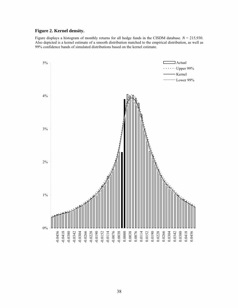
38

Figure 2. Kernel density. Figure displays a histogram of monthly returns for all hedge funds in the CISDM database. N = 215,930. Also depicted is a kernel estimate of a smooth distribution matched to the empirical distribution, as well as 99% confidence bands of simulated distributions based on the kernel estimate.

0%

1%

2%

3%

4%

5%-0

.045

6-0

.041

8-0

.038

0-0

.034

2-0

.030

4-0

.026

6-0

.022

8-0

.019

0-0

.015

2-0

.011

4-0

.007

6-0

.003

80.

0000

0.00

380.

0076

0.01

140.

0152

0.01

900.

0228

0.02

660.

0304

0.03

420.

0380

0.04

180.

0456

ActualUpper 99%KernelLower 99%

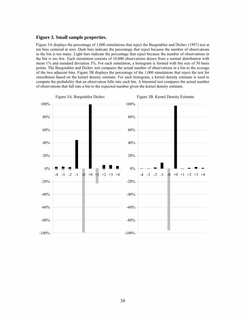
39

Figure 3. Small sample properties. Figure 3A displays the percentage of 1,000 simulations that reject the Burgstahler and Dichev (1997) test at ten bins centered at zero. Dark bars indicate the percentage that reject because the number of observations in the bin is too many. Light bars indicate the percentage that reject because the number of observations in the bin is too few. Each simulation consists of 10,000 observations drawn from a normal distribution with mean 1% and standard deviation 3%. For each simulation, a histogram is formed with bin size of 50 basis points. The Burgstahler and Dichev test compares the actual number of observations in a bin to the average of the two adjacent bins. Figure 3B displays the percentage of the 1,000 simulations that reject the test for smoothness based on the kernel density estimate. For each histogram, a kernel density estimate is used to compute the probability that an observation falls into each bin. A binomial test compares the actual number of observations that fall into a bin to the expected number given the kernel density estimate.

Figure 3A. Burgstahler Dichev Figure 3B. Kernel Density Estimate

-100%

-80%

-60%

-40%

-20%

0%

20%

40%

60%

80%

100%

-4 -3 -2 -1 -0 +0 +1 +2 +3 +4

-100%

-80%

-60%

-40%

-20%

0%

20%

40%

60%

80%

100%

-4 -3 -2 -1 -0 +0 +1 +2 +3 +4

40

Figure 4. Stock returns. Figures 4A, 4B, and 4C show histograms of monthly returns of individual NASDAQ and AMEX/NYSE stocks over three periods defined by tick size regime: eighths, sixteenths, and decimals, respectively. Bold vertical bars indicate returns bracketing zero.

NASDAQ NSYEFigure 4C. April 2001 - December 2005

NASDAQ NSYEFigure 4A. January 1994 - May 1997

NASDAQ NSYEFigure 4B. July 1997 - August 2000

0%

1%

2%

3%

4%

5%

-0.2

751

-0.2

522

-0.2

292

-0.2

063

-0.1

834

-0.1

605

-0.1

375

-0.1

146

-0.0

917

-0.0

688

-0.0

458

-0.0

229

0.00

000.

0229

0.04

580.

0688

0.09

170.

1146

0.13

750.

1605

0.18

340.

2063

0.22

920.

2522

0.27

51

0%

1%

2%

3%

4%

5%

-0.2

650

-0.2

429

-0.2

208

-0.1

987

-0.1

767

-0.1

546

-0.1

325

-0.1

104

-0.0

883

-0.0

662

-0.0

442

-0.0

221

0.00

000.

0221

0.04

420.

0662

0.08

830.

1104

0.13

250.

1546

0.17

670.

1987

0.22

080.

2429

0.26

50

0%

1%

2%

3%

4%

5%

-0.3

493

-0.3

202

-0.2

911

-0.2

620

-0.2

329

-0.2

038

-0.1

747

-0.1

456

-0.1

164

-0.0

873

-0.0

582

-0.0

291

0.00

000.

0291

0.05

820.

0873

0.11

640.

1456

0.17

470.

2038

0.23

290.

2620

0.29

110.

3202

0.34

93

0%

1%

2%

3%

4%

5%

-0.1

735

-0.1

591

-0.1

446

-0.1

302

-0.1

157

-0.1

012

-0.0

868

-0.0

723

-0.0

578

-0.0

434

-0.0

289

-0.0

145

0.00

000.

0145

0.02

890.

0434

0.05

780.

0723

0.08

680.

1012

0.11

570.

1302

0.14

460.

1591

0.17

350%

1%

2%

3%

4%

5%

-0.2

266

-0.2

077

-0.1

888

-0.1

699

-0.1

510

-0.1

322

-0.1

133

-0.0

944

-0.0

755

-0.0

566

-0.0

378

-0.0

189

0.00

000.

0189

0.03

780.

0566

0.07

550.

0944

0.11

330.

1322

0.15

100.

1699

0.18

880.

2077

0.22

66

0%

1%

2%

3%

4%

5%

-0.1

588

-0.1

456

-0.1

323

-0.1

191

-0.1

059

-0.0

926

-0.0

794

-0.0

662

-0.0

529

-0.0

397

-0.0

265

-0.0

132

0.00

000.

0132

0.02

650.

0397

0.05

290.

0662

0.07

940.

0926

0.10

590.

1191

0.13

230.

1456

0.15

88

41

Figure 5. Mutual fund returns. Histograms of monthly returns of all equity mutual funds in the CRSP database. Bold vertical bars indicate returns bracketing zero.

20052002

2000 2003

2001 2004

1994

1995

1996

1997

1998

1999

0%

1%

2%

3%

4%

5%

6%

7%

8%

-0.1

272

-0.1

166

-0.1

060

-0.0

954

-0.0

848

-0.0

742

-0.0

636

-0.0

530

-0.0

424

-0.0

318

-0.0

212

-0.0

106

0.00

000.

0106

0.02

120.

0318

0.04

240.

0530

0.06

360.

0742

0.08

480.

0954

0.10

600.

1166

0.12

72

0%

1%

2%

3%

4%

5%

6%

7%

8%

-0.0

903

-0.0

834

-0.0

764

-0.0

695

-0.0

625

-0.0

556

-0.0

486

-0.0

417

-0.0

347

-0.0

278

-0.0

208

-0.0

139

-0.0

069

0.00

000.

0069

0.01

390.

0208

0.02

780.

0347

0.04

170.

0486

0.05

560.

0625

0.06

950.

0764

0.08

34

0%

1%

2%

3%

4%

5%

6%

7%

8%

-0.1

288

-0.1

188

-0.1

089

-0.0

990

-0.0

891

-0.0

792

-0.0

693

-0.0

594

-0.0

495

-0.0

396

-0.0

297

-0.0

198

-0.0

099

0.00

000.

0099

0.01

980.

0297

0.03

960.

0495

0.05

940.

0693

0.07

920.

0891

0.09

900.

1089

0.11

88

0%

1%

2%

3%

4%

5%

6%

7%

8%

-0.1

963

-0.1

812

-0.1

661

-0.1

510

-0.1

359

-0.1

208

-0.1

057

-0.0

906

-0.0

755

-0.0

604

-0.0

453

-0.0

302

-0.0

151

0.00

000.

0151

0.03

020.

0453

0.06

040.

0755

0.09

060.

1057

0.12

080.

1359

0.15

100.

1661

0.18

12

0%

1%

2%

3%

4%

5%

6%

7%

8%

-0.2

290

-0.2

114

-0.1

938

-0.1

761

-0.1

585

-0.1

409

-0.1

233

-0.1

057

-0.0

881

-0.0

705

-0.0

528

-0.0

352

-0.0

176

0.00

000.

0176

0.03

520.

0528

0.07

050.

0881

0.10

570.

1233

0.14

090.

1585

0.17

610.

1938

0.21

14

0%

1%

2%

3%

4%

5%

6%

7%

8%

-0.2

158

-0.1

992

-0.1

826

-0.1

660

-0.1

494

-0.1

328

-0.1

162

-0.0

996

-0.0

830

-0.0

664

-0.0

498

-0.0

332

-0.0

166

0.00

000.

0166

0.03

320.

0498

0.06

640.

0830

0.09

960.

1162

0.13

280.

1494

0.16

600.

1826

0.19

92

0%

1%

2%

3%

4%

5%

6%

7%

8%

-0.2

652

-0.2

448

-0.2

244

-0.2

040

-0.1

836

-0.1

632

-0.1

428

-0.1

224

-0.1

020

-0.0

816

-0.0

612

-0.0

408

-0.0

204

0.00

000.

0204

0.04

080.

0612

0.08

160.

1020

0.12

240.

1428

0.16

320.

1836

0.20

400.

2244

0.24

48

0%

1%

2%

3%

4%

5%

6%

7%

8%

-0.2

689

-0.2

482

-0.2

275

-0.2

069

-0.1

862

-0.1

655

-0.1

448

-0.1

241

-0.1

034

-0.0

827

-0.0

621

-0.0

414

-0.0

207

0.00

000.

0207

0.04

140.

0621

0.08

270.

1034

0.12

410.

1448

0.16

550.

1862

0.20

690.

2275

0.24

82

0%

1%

2%

3%

4%

5%

6%

7%

8%

-0.2

275

-0.2

100

-0.1

925

-0.1

750

-0.1

575

-0.1

400

-0.1

225

-0.1

050

-0.0

875

-0.0

700

-0.0

525

-0.0

350

-0.0

175

0.00

000.

0175

0.03

500.

0525

0.07

000.

0875

0.10

500.

1225

0.14

000.

1575

0.17

500.

1925

0.21

00

0%

1%

2%

3%

4%

5%

6%

7%

8%

-0.1

421

-0.1

312

-0.1

202

-0.1

093

-0.0

984

-0.0

874

-0.0

765

-0.0

656

-0.0

547

-0.0

437

-0.0

328

-0.0

219

-0.0

109

0.00

000.

0109

0.02

190.

0328

0.04

370.

0547

0.06

560.

0765

0.08

740.

0984

0.10

930.

1202

0.13

12

0%

1%

2%

3%

4%

5%

6%

7%

8%

-0.1

025

-0.0

946

-0.0

867

-0.0

788

-0.0

709

-0.0

631

-0.0

552

-0.0

473

-0.0

394

-0.0

315

-0.0

236

-0.0

158

-0.0

079

0.00

000.

0079

0.01

580.

0236

0.03

150.

0394

0.04

730.

0552

0.06

310.

0709

0.07

880.

0867

0.09

46

0%

1%

2%

3%

4%

5%

6%

7%

8%

-0.1

313

-0.1

212

-0.1

111

-0.1

010

-0.0

909

-0.0

808

-0.0

707

-0.0

606

-0.0

505

-0.0

404

-0.0

303

-0.0

202

-0.0

101

0.00

000.

0101

0.02

020.

0303

0.04

040.

0505

0.06

060.

0707

0.08

080.

0909

0.10

100.

1111

0.12

12

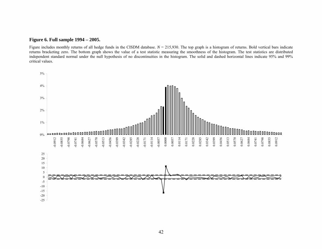
42

Figure 6. Full sample 1994 – 2005. Figure includes monthly returns of all hedge funds in the CISDM database. N = 215,930. The top graph is a histogram of returns. Bold vertical bars indicate returns bracketing zero. The bottom graph shows the value of a test statistic measuring the smoothness of the histogram. The test statistics are distributed independent standard normal under the null hypothesis of no discontinuities in the histogram. The solid and dashed horizontal lines indicate 95% and 99% critical values.

0%

1%

2%

3%

4%

5%

-0.0

912

-0.0

855

-0.0

798

-0.0

741

-0.0

684

-0.0

627

-0.0

570

-0.0

513

-0.0

456

-0.0

399

-0.0

342

-0.0

285

-0.0

228

-0.0

171

-0.0

114

-0.0

057

0.00

00

0.00

57

0.01

14

0.01

71

0.02

28

0.02

85

0.03

42

0.03

99

0.04

56

0.05

13

0.05

70

0.06

27

0.06

84

0.07

41

0.07

98

0.08

55

0.09

12

-25-20-15-10

-505

10152025

43

Figure 7. Audit versus non-audit months. Figure 7A includes months during which an audit occurred and the prior two months, N = 1,908. Figure 7B includes observations from funds with no audit dates, N = 15,574. Observations match the date, strategy, and size quintile of observations in Figure 7A.The top graph is a histogram of returns. Bold vertical bars indicate returns bracketing zero. The bottom graph shows the value of a test statistic measuring the smoothness of the histogram. The test statistics are distributed independent standard normal under the null hypothesis of no discontinuities in the histogram.

Figure 7A. Audit Months Figure 7B. Non-audit Months

0%

2%

4%

6%

8%

10%

12%

-0.0

720

-0.0

660

-0.0

600

-0.0

540

-0.0

480

-0.0

420

-0.0

360

-0.0

300

-0.0

240

-0.0

180

-0.0

120

-0.0

060

0.00

000.

0060

0.01

200.

0180

0.02

400.

0300

0.03

600.

0420

0.04

800.

0540

0.06

000.

0660

0.07

20

-5-4-3-2-1012345

0%

2%

4%

6%

8%

10%

12%

-0.0

840

-0.0

770

-0.0

700

-0.0

630

-0.0

560

-0.0

490

-0.0

420

-0.0

350

-0.0

280

-0.0

210

-0.0

140

-0.0

070

0.00

000.

0070

0.01

400.

0210

0.02

800.

0350

0.04

200.

0490

0.05

600.

0630

0.07

000.

0770

0.08

40

-5-4-3-2-1012345

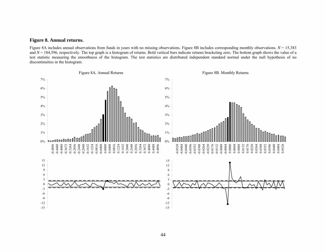
44

Figure 8. Annual returns. Figure 8A includes annual observations from funds in years with no missing observations. Figure 8B includes corresponding monthly observations. N = 15,383 and N = 184,596, respectively. The top graph is a histogram of returns. Bold vertical bars indicate returns bracketing zero. The bottom graph shows the value of a test statistic measuring the smoothness of the histogram. The test statistics are distributed independent standard normal under the null hypothesis of no discontinuities in the histogram.

Figure 8A. Annual Returns Figure 8B. Monthly Returns

0%

1%

2%

3%

4%

5%

6%

7%

-0.4

896

-0.4

488

-0.4

080

-0.3

672

-0.3

264

-0.2

856

-0.2

448

-0.2

040

-0.1

632

-0.1

224

-0.0

816

-0.0

408

0.00

000.

0408

0.08

160.

1224

0.16

320.

2040

0.24

480.

2856

0.32

640.

3672

0.40

800.

4488

0.48

96

-15-12

-9-6-30369

1215

0%

1%

2%

3%

4%

5%

6%

7%

-0.0

528

-0.0

484

-0.0

440

-0.0

396

-0.0

352

-0.0

308

-0.0

264

-0.0

220

-0.0

176

-0.0

132

-0.0

088

-0.0

044

0.00

000.

0044

0.00

880.

0132

0.01

760.

0220

0.02

640.

0308

0.03

520.

0396

0.04

400.

0484

0.05

28

-15-12

-9-6-30369

1215

45

Figure 9. Factor models. Figures 9A and 9B include observations of raw hedge fund returns as well as fitted returns from linear factor models. N = 200,500 in both cases. The top graph is a histogram of returns. Bold vertical bars indicate returns bracketing zero. The bottom graph shows the value of a test statistic measuring the smoothness of the histogram. The test statistics are distributed independent standard normal under the null hypothesis of no discontinuities in the histogram.

Figure 9A. Raw Returns Figure 9B. Fitted Returns

-20-16-12

-8-4048

121620

0%

1%

2%

3%

4%

5%

-0.0

464

-0.0

426

-0.0

387

-0.0

348

-0.0

310

-0.0

271

-0.0

232

-0.0

193

-0.0

155

-0.0

116

-0.0

077

-0.0

039

0.00

000.

0039

0.00

770.

0116

0.01

550.

0193

0.02

320.

0271

0.03

100.

0348

0.03

870.

0426

0.04

64

0%

1%

2%

3%

4%

5%

-0.0

277

-0.0

254

-0.0

231

-0.0

207

-0.0

184

-0.0

161

-0.0

138

-0.0

115

-0.0

092

-0.0

069

-0.0

046

-0.0

023

0.00

000.

0023

0.00

460.

0069

0.00

920.

0115

0.01

380.

0161

0.01

840.

0207

0.02

310.

0254

0.02

77

-20-16-12

-8-4048

121620

46

Figure 10. CTAs versus hedge funds. Figures 10A and 10B include monthly returns of all CTAs and hedge funds in the CISDM database. N = 64,562 and N = 215,930, respectively. Bold vertical bars indicate returns bracketing zero.

Figure 10A. CTAs

0%1%2%3%4%5%6%7%8%9%

-0.1

84

-0.1

72

-0.1

61

-0.1

49

-0.1

38

-0.1

26

-0.1

15

-0.1

03

-0.0

92

-0.0

80

-0.0

69

-0.0

57

-0.0

46

-0.0

34

-0.0

23

-0.0

11

0.00

0

0.01

1

0.02

3

0.03

4

0.04

6

0.05

7

0.06

9

0.08

0

0.09

2

0.10

3

0.11

5

0.12

6

0.13

8

0.14

9

0.16

1

0.17

2

0.18

4

Figure 10B. Hedge Funds

0%1%2%3%4%5%6%7%8%9%

-0.1

84

-0.1

72

-0.1

61

-0.1

49

-0.1

38

-0.1

26

-0.1

15

-0.1

03

-0.0

92

-0.0

80

-0.0

69

-0.0

57

-0.0

46

-0.0

34

-0.0

23

-0.0

11

0.00

0

0.01

1

0.02

3

0.03

4

0.04

6

0.05

7

0.06

9

0.08

0

0.09

2

0.10

3

0.11

5

0.12

6

0.13

8

0.14

9

0.16

1

0.17

2

0.18

4

47

Figure 11. Estimated number of distorted returns. Listed are estimates of the number of hedge fund returns that have been distorted. Estimates are computed from comparing the frequency of observing returns in different bins across the pooled distributions of CTA returns and hedge fund returns.

-2,000-1,000

01,0002,0003,0004,0005,0006,0007,0008,000

-0.1

84

-0.1

72

-0.1

61

-0.1

49

-0.1

38

-0.1

26

-0.1

15

-0.1

03

-0.0

92

-0.0

80

-0.0

69

-0.0

57

-0.0

46

-0.0

34

-0.0

23

-0.0

11

0.00

0

0.01

1

0.02

3

0.03

4

0.04

6

0.05

7

0.06

9

0.08

0

0.09

2

0.10

3

0.11

5

0.12

6

0.13

8

0.14

9

0.16

1

0.17

2

0.18

4

48

Figure 12. Smoothing profiles. Figures 12A and 12B include observations from funds in the bottom and top quartiles as measured by return smoothing. N = 31,981 and N = 31,166, respectively. The top graph is a histogram of returns. Bold vertical bars indicate returns bracketing zero. The bottom graph shows the value of a test statistic measuring the smoothness of the histogram. The test statistics are distributed independent standard normal under the null hypothesis of no discontinuities in the histogram.

Figure 12B. High SmoothingFigure 12A. Low Smoothing

0%

1%

2%

3%

4%

5%

6%

7%

-0.0

408

-0.0

374

-0.0

340

-0.0

306

-0.0

272

-0.0

238

-0.0

204

-0.0

170

-0.0

136

-0.0

102

-0.0

068

-0.0

034

0.00

000.

0034

0.00

680.

0102

0.01

360.

0170

0.02

040.

0238

0.02

720.

0306

0.03

400.

0374

0.04

08

-10-8-6-4-202468

10

0%

1%

2%

3%

4%

5%

6%

7%

-0.0

960

-0.0

880

-0.0

800

-0.0

720

-0.0

640

-0.0

560

-0.0

480

-0.0

400

-0.0

320

-0.0

240

-0.0

160

-0.0

080

0.00

000.

0080

0.01

600.

0240

0.03

200.

0400

0.04

800.

0560

0.06

400.

0720

0.08

000.

0880

0.09

60

-10-8-6-4-202468

10

49

Figure 13. Discontinuity by strategy. Figures 13A and 13B include observations from funds in the Equity Market Neutral and Distressed Securities categories. N = 10,855 and N = 7,840, respectively. The top graph is a histogram of returns. Bold vertical bars indicate returns bracketing zero. The bottom graph shows the value of a test statistic measuring the smoothness of the histogram. The test statistics are distributed independent standard normal under the null hypothesis of no discontinuities in the histogram.

Figure 13A. Equity Market Neutral Figure 13B. Distressed Securities

0%

1%

2%

3%

4%

5%

6%

7%

8%

-0.0

624

-0.0

572

-0.0

520

-0.0

468

-0.0

416

-0.0

364

-0.0

312

-0.0

260

-0.0

208

-0.0

156

-0.0

104

-0.0

052

0.00

000.

0052

0.01

040.

0156

0.02

080.

0260

0.03

120.

0364

0.04

160.

0468

0.05

200.

0572

0.06

24

-5-4-3-2-1012345

0%

1%

2%

3%

4%

5%

6%

7%

8%

-0.0

552

-0.0

506

-0.0

460

-0.0

414

-0.0

368

-0.0

322

-0.0

276

-0.0

230

-0.0

184

-0.0

138

-0.0

092

-0.0

046

0.00

000.

0046

0.00

920.

0138

0.01

840.

0230

0.02

760.

0322

0.03

680.

0414

0.04

600.

0506

0.05

52

-5-4-3-2-1012345

50

Figure 14. Defunct versus live funds. Figures 14A and 14B include defunct and live funds. In all cases, the first 12 observations for each fund are dropped. N = 79,426 and N = 87,822, respectively. The top graph is a histogram of returns. Bold vertical bars indicate returns bracketing zero. The bottom graph shows the value of a test statistic measuring the smoothness of the histogram. The test statistics are distributed independent standard normal under the null hypothesis of no discontinuities in the histogram.

Figure 14A. Defunct Funds Figure 14B. Live Funds

0%

1%

2%

3%

4%

5%

6%

-0.0

624

-0.0

572

-0.0

520

-0.0

468

-0.0

416

-0.0

364

-0.0

312

-0.0

260

-0.0

208

-0.0

156

-0.0

104

-0.0

052

0.00

000.

0052

0.01

040.

0156

0.02

080.

0260

0.03

120.

0364

0.04

160.

0468

0.05

200.

0572

0.06

24

-20-16-12

-8-4048

121620

0%

1%

2%

3%

4%

5%

6%

-0.0

504

-0.0

462

-0.0

420

-0.0

378

-0.0

336

-0.0

294

-0.0

252

-0.0

210

-0.0

168

-0.0

126

-0.0

084

-0.0

042

0.00

000.

0042

0.00

840.

0126

0.01

680.

0210

0.02

520.

0294

0.03

360.

0378

0.04

200.

0462

0.05

04

-20-16-12

-8-4048

121620

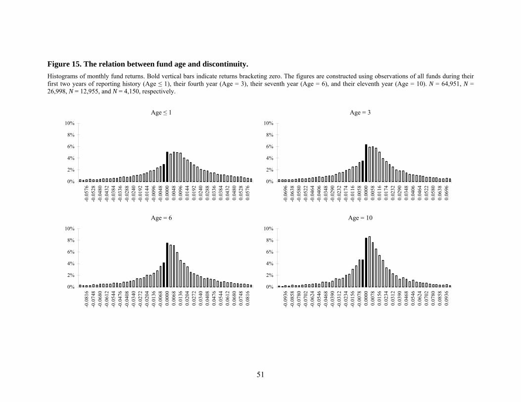
51

Figure 15. The relation between fund age and discontinuity. Histograms of monthly fund returns. Bold vertical bars indicate returns bracketing zero. The figures are constructed using observations of all funds during their first two years of reporting history (Age ≤ 1), their fourth year (Age = 3), their seventh year (Age = 6), and their eleventh year (Age = 10). N = 64,951, N = 26,998, N = 12,955, and N = 4,150, respectively.

Age ≤ 1 Age = 3

Age = 6 Age = 10

0%

2%

4%

6%

8%

10%

-0.0

576

-0.0

528

-0.0

480

-0.0

432

-0.0

384

-0.0

336

-0.0

288

-0.0

240

-0.0

192

-0.0

144

-0.0

096

-0.0

048

0.00

000.

0048

0.00

960.

0144

0.01

920.

0240

0.02

880.

0336

0.03

840.

0432

0.04

800.

0528

0.05

76

0%

2%

4%

6%

8%

10%

-0.0

696

-0.0

638

-0.0

580

-0.0

522

-0.0

464

-0.0

406

-0.0

348

-0.0

290

-0.0

232

-0.0

174

-0.0

116

-0.0

058

0.00

000.

0058

0.01

160.

0174

0.02

320.

0290

0.03

480.

0406

0.04

640.

0522

0.05

800.

0638

0.06

96

0%

2%

4%

6%

8%

10%

-0.0

816

-0.0

748

-0.0

680

-0.0

612

-0.0

544

-0.0

476

-0.0

408

-0.0

340

-0.0

272

-0.0

204

-0.0

136

-0.0

068

0.00

000.

0068

0.01

360.

0204

0.02

720.

0340

0.04

080.

0476

0.05

440.

0612

0.06

800.

0748

0.08

16

0%

2%

4%

6%

8%

10%

-0.0

936

-0.0

858

-0.0

780

-0.0

702

-0.0

624

-0.0

546

-0.0

468

-0.0

390

-0.0

312

-0.0

234

-0.0

156

-0.0

078

0.00

000.

0078

0.01

560.

0234

0.03

120.

0390

0.04

680.

0546

0.06

240.

0702

0.07

800.

0858

0.09

36

52

Figure 16. The relation between fund age and discontinuity. The figures show the value of a test statistic measuring the smoothness of the histograms of monthly fund returns. The test statistic is distributed standard normal under the null hypothesis of no discontinuities in the histogram. The two values to the left and right of a zero return are indicated by solid squares. The figures are constructed using observations of all funds during their first two years of reporting history (Age ≤ 1), their fourth year (Age = 3), their seventh year (Age = 6), and their eleventh year (Age = 10). N = 64,951, N = 26,998, N = 12,955, and N = 4,150, respectively.

Age ≤ 1 Age = 3

Age = 6 Age = 10

-15-12

-9-6-30369

1215

-15-12

-9-6-30369

1215

-15-12

-9-6-30369

1215

-15-12

-9-6-30369

1215

53

Figure 17. December versus January returns. Figures 17A and 17B include returns from December and January. N = 18,590 and N = 17,411, respectively. The top graph is a histogram of returns. Bold vertical bars indicate returns bracketing zero. The bottom graph shows the value of a test statistic measuring the smoothness of the histogram. The test statistics are distributed independent standard normal under the null hypothesis of no discontinuities in the histogram.

Figure 17A. December Returns Figure 17B. January Returns

0%

1%

2%

3%

4%

5%

6%

7%

8%

-0.0

744

-0.0

682

-0.0

620

-0.0

558

-0.0

496

-0.0

434

-0.0

372

-0.0

310

-0.0

248

-0.0

186

-0.0

124

-0.0

062

0.00

000.

0062

0.01

240.

0186

0.02

480.

0310

0.03

720.

0434

0.04

960.

0558

0.06

200.

0682

0.07

44

-6-5-4-3-2-10123456

0%

1%

2%

3%

4%

5%

6%

7%

8%

-0.0

696

-0.0

638

-0.0

580

-0.0

522

-0.0

464

-0.0

406

-0.0

348

-0.0

290

-0.0

232

-0.0

174

-0.0

116

-0.0

058

0.00

000.

0058

0.01

160.

0174

0.02

320.

0290

0.03

480.

0406

0.04

640.

0522

0.05

800.

0638

0.06

96

-6-5-4-3-2-10123456

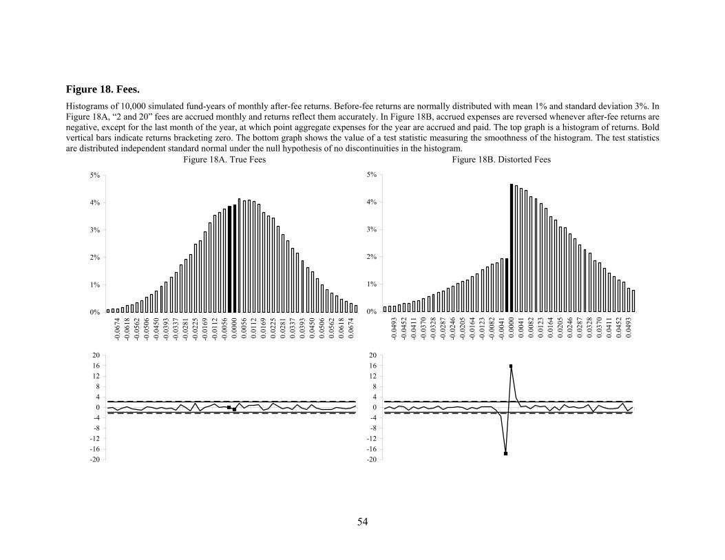
54

Figure 18. Fees. Histograms of 10,000 simulated fund-years of monthly after-fee returns. Before-fee returns are normally distributed with mean 1% and standard deviation 3%. In Figure 18A, “2 and 20” fees are accrued monthly and returns reflect them accurately. In Figure 18B, accrued expenses are reversed whenever after-fee returns are negative, except for the last month of the year, at which point aggregate expenses for the year are accrued and paid. The top graph is a histogram of returns. Bold vertical bars indicate returns bracketing zero. The bottom graph shows the value of a test statistic measuring the smoothness of the histogram. The test statistics are distributed independent standard normal under the null hypothesis of no discontinuities in the histogram.

Figure 18A. True Fees Figure 18B. Distorted Fees

0%

1%

2%

3%

4%

5%

-0.0

674

-0.0

618

-0.0

562

-0.0

506

-0.0

450

-0.0

393

-0.0

337

-0.0

281

-0.0

225

-0.0

169

-0.0

112

-0.0

056

0.00

000.

0056

0.01

120.

0169

0.02

250.

0281

0.03

370.

0393

0.04

500.

0506

0.05

620.

0618

0.06

74

0%

1%

2%

3%

4%

5%

-0.0

493

-0.0

452

-0.0

411

-0.0

370

-0.0

328

-0.0

287

-0.0

246

-0.0

205

-0.0

164

-0.0

123

-0.0

082

-0.0

041

0.00

000.

0041

0.00

820.

0123

0.01

640.

0205

0.02

460.

0287

0.03

280.

0370

0.04

110.

0452

0.04

93

-20-16-12

-8-4048

121620

-20-16-12

-8-4048

121620