What can be learned from gravitational-waves on the physics of bursts and compact binaries

Vivien Raymond for LIGO Scientific collaboration and Virgo collaboration

LIGO DCC G140082610th Rencontres du Vietnam August 3 - 9, 2014 ICISE, Quy Nhon, Vietnam

Quantum fluctuations in the early universe

Binary Supermassive Black Holes in the galactic nuclei

Compact Binary Coalescences

Rotating NS, Supernovae

Compact objects captured by

Supermassive Black Holes

Cosmic microwave background polarization

Space Interferometers

Ground Interferometers

Pulsar Timing

years hours sec msage of the universewave period

log(frequency)

Sour

ces

Dete

ctor

s

-16 -14 -12 -10 -8 -6 -4 -2 0 +2

The Gravitational Wave Spectrum

[Inspired from http://science.gsfc.nasa.gov/663/research/] 2

Gravitational Wave Astronomy

• Gravitational wave detectors will study sources characterised by extreme physical conditions: strong non-linear gravity and relativistic motions, very high densities, …

!

!

!

• Here are some examples of questions which will hopefully be answered:

3

[Image: NASA/CXC/GSFC/T.Strohmayer]

Fundamental physics:

• What are the properties of gravitational waves?

• Is General Relativity still valid under strong-gravity conditions?

• Are nature’s black holes the black holes of General Relativity?

• How does matter behave under extremes of density and pressure?

4

Astrophysics

• How abundant are stellar-mass binary black holes?

• Is the mechanism that generates gamma-ray bursts a compact binary coalescence?

• How do compact binary stars form and evolve, and what has been their effect on star formation rates?

• Where and when do massive black holes form, and what role do they play in the formation and evolution of galaxies?

• What happens when a massive star collapses?

5

Prediction for Detection Rates

7

TABLE IV: Compact binary coalescence rates per Mpc3 per Myr.a

Source Rlow Rre Rhigh Rmax

NS-NS (Mpc−3 Myr−1) 0.01 [1] 1 [1] 10 [1] 50 [16]NS-BH (Mpc−3 Myr−1) 6× 10−4 [18] 0.03 [18] 1 [18]BH-BH (Mpc−3 Myr−1) 1× 10−4 [14] 0.005 [14] 0.3 [14]

aSee footnotes in Table II for details on the sources of the values in this Table

TABLE V: Detection rates for compact binary coalescence sources.

IFO Sourcea Nlow Nre Nhigh Nmax

yr−1 yr−1 yr−1 yr−1

NS-NS 2× 10−4 0.02 0.2 0.6NS-BH 7× 10−5 0.004 0.1

Initial BH-BH 2× 10−4 0.007 0.5IMRI into IMBH < 0.001b 0.01c

IMBH-IMBH 10−4d 10−3e

NS-NS 0.4 40 400 1000NS-BH 0.2 10 300

Advanced BH-BH 0.4 20 1000IMRI into IMBH 10b 300c

IMBH-IMBH 0.1d 1e

aTo convert the rates per MWEG in Table II into detection rates, optimal horizon distances of 33 Mpc / 445 Mpc are assumed for NS-NSinspirals in the Initial / Advanced LIGO-Virgo networks. For NS-BH inspirals, horizon distances of 70 Mpc / 927 Mpc are assumed. ForBH-BH inspirals, horizon distances of 161 Mpc / 2187 Mpc are assumed. These distances correspond to a choice of 1.4 M⊙ for NS massand 10 M⊙ for BH mass. Rates for IMRIs into IMBHs and IMBH-IMBH coalescences are quoted directly from the relevant papers withoutconversion. See Section III for more details.bRate taken from the estimate of BH-IMBH IMRI rates quoted in [19] for the scenario of BH-IMBH binary hardening via 3-body

interactions; the fraction of globular clusters containing suitable IMBHs is taken to be 10%, and no interferometer optimizations areassumed.cRate taken from the optimistic upper limit rate quoted in [19] with the assumption that all globular clusters contain suitable IMBHs;

for the Advanced network rate, the interferometer is assumed to be optimized for IMRI detections.dRate taken from the estimate of IMBH-IMBH ringdown rates quoted in [20] assuming 10% of all young star clusters have sufficient

mass, a sufficiently high binary fraction, and a short enough core collapse time to form a pair of IMBHs.eRate taken from the estimate of IMBH-IMBH ringdown rates quoted in [20] assuming all young star clusters have sufficient mass, a

sufficiently high binary fraction, and a short enough core collapse time to form a pair of IMBHs.

III. CONVERSION FROM MERGER RATES TO DETECTION RATES

Although some publications quote detection rates for Initial and Advanced LIGO-Virgo networks directly, theconversion from coalescence rates per galaxy to detection rates is not consistent across all publications. Therefore,we choose to re-compute the detection rates as follows.4

The actual detection threshold for a network of interferometers will depend on a number of factors, including thenetwork configuration (the relative locations, orientations, and noise power spectral densities of the detectors), thecharacteristics of the detector noise (its Gaussianity and stationarity), and the search strategy used (coincident vs.coherent search) (see, e.g., [24]). A full treatment of these effects is beyond the scope of this paper. Instead, weestimate event rates detectable by the LIGO-Virgo network by scaling to an average volume within which a singledetector is sensitive to CBCs above a fiducial signal-to-noise ratio (SNR) threshold of 8. This is a conservative choiceif the detector noise is Gaussian and stationary and if there are two or more detectors operating in coincidence.5

4 Rates of IMRIs into IMBHs and IMBH-IMBH coalescences are an exception: because of the many assumptions involved in convertingrates per globular cluster into LIGO-Virgo detection rates, we quote detection rates for these sources directly as they appear in therelevant publications.

5 The real detection range of the network is a function of the data quality and the detection pipeline, and can only be obtained empirically.However, we can argue that our choice is not unreasonable as follows. We compute below that the NS-NS horizon distance for theInitial-era interferometers is Dhorizon = 33 Mpc. According to Eq. (5), this corresponds to an accessible volume of ∼ 150 MWEGs or∼ 250 L10. Meanwhile, the 90%-confidence upper limit on NS-NS rates from a year and a half of data (including approximately half

[Abadie et al., Class. Quant. Grav.27:173001 (2010)]

6

Upper Limits

[Abadie et al., PRD 85, 082002 (2012)]

10

2.0 5.0 8.0 11.0 14.0 17.0 20.0 25.0

Total Mass (M�)

10�6

10�5

10�4

Rat

e(M

pc�

3yr

�1)

3.0 8.0 13.0 18.0 23.0

Component Mass (M�)

10�5

10�4

Rat

e(M

pc�

3yr

�1)

FIG. 4: The marginalized upper limits as a function of mass.The top plot shows the limit as a function of total mass M ,using a distribution uniform in m

1

for a given M . The lowerplot shows the limit as a function of the black hole mass, withthe neutron star mass restricted to the range 1� 3M�. Thelight bars indicate upper limits from previous searches. Thedark bars indicate the combined upper limits including theresults of this search.

spinning. Signals from spinning systems are recoveredwith a worse match to our templates since we use a non-spinning template bank.

While the rates presented here represent an improve-ment over the previously published results from ear-lier LIGO and Virgo science runs, they are still abovethe astrophysically predicted rates of binary coalescence.There are numerous uncertainties involved in estimat-ing astrophysical rates, including limited numbers ofobservations and unknown model parameters; conse-quently the rate estimates are rather uncertain. ForBNS systems the estimated rates vary between 1 ⇥ 10�8

and 1 ⇥ 10�5 Mpc�3yr�1, with a “realistic” estimateof 1 ⇥ 10�6 Mpc�3yr�1. For BBH and NSBH, realis-tic estimates of the rate are 5 ⇥ 10�9 Mpc�3yr�1 and

BNS NSBH BBH

10�10

10�9

10�8

10�7

10�6

10�5

10�4

10�3

Rat

eE

stim

ates

� Mpc�

3 yr�

1�

FIG. 5: Comparison of CBC upper limit rates for BNS, NSBHand BBH systems. The light gray regions display the upperlimits obtained in the S5-VSR1 analysis; dark gray regionsshow the upper limits obtained in this analysis, using the S5-VSR1 limits as priors. The new limits are up to a factor of1.4 improvement over the previous results. The lower (blue)regions show the spread in the astrophysically predicted rates,with the dashed-black lines showing the “realistic” estimates[5]. Note: In [5], NSBH and BBH rates were quoted using ablack-hole mass of 10M�. We have therefore rescaled the S5and S6 NSBH and BBH upper limits in this plot by a factorof (M

5

/M10

)5/2, where M10

is the chirp mass of a binary inwhich the black hole mass is 10M� and M

5

is the chirp massof a binary in which the black hole mass is 5M�.

3 ⇥ 10�8 Mpc�3yr�1 with at least an order of magnitudeuncertainty in either direction [5]. In all cases, the upperlimits derived here are two to three orders of magnitudeabove the “realistic” estimated rates, and about a fac-tor of ten above the most optimistic predictions. Theseresults are summarized in Figure 5.

VII. DISCUSSION

We performed a search for gravitational waves fromcompact binary coalescences with total mass between 2and 25 M� with the LIGO and Virgo detectors usingdata taken between July 7, 2009 and October 20, 2010.No gravitational waves candidates were detected, and weplaced new upper limits on CBC rates. These new limitsare up to a factor of 1.4 improvement over those achievedusing previous LIGO and Virgo observational runs up toS5/VSR1 [4], but remain two to three orders of magni-tude above the astrophysically predicted rates.

The installation of the advanced LIGO and Virgo de-tectors has begun. When operational, these detectors willprovide a factor of ten increase in sensitivity over the ini-tial detectors, providing a factor of ⇠ 1000 increase inthe sensitive volume. At that time, we expect to observetens of binary coalescences per year [5].

In order to detect this population of gravitational wave

7

• No inspiral signals detected

• 90% confidence limits on coalescence rates:

• For binary neutron stars: < 1.3×10–4 Mpc-3 yr-1

• For binary black holes with 5+5M⊙: < 6.4×10–6 Mpc-3 yr-1

• Soon to confront expected range of merger rates

2018 Preview

8

source current upper limit 2nd gen rate predicted rateneutron star binaries

(1.35 + 1.35 M⊙) 1.3x10-4 Mpc-3 yr-1 1.3 ⨉ 10-7 Mpc-3 yr-1 10-6 Mpc-3 yr-1

stellar mass BH binaries(5 + 5 M⊙) 6.4 ⨉ 10-6 Mpc-3 yr-1 6.4 ⨉ 10-9 Mpc-3 yr-1 5 ⨉ 10-9 Mpc-3 yr-1

mixed binaries(1.35 + 5 M⊙) 3.1 ⨉ 10-5 Mpc-3 yr-1 3.1 ⨉ 10-8 Mpc-3 yr-1 3 ⨉ 10-8 Mpc-3 yr-1

“high stellar mass” BH binaries(50 + 50 M⊙) 7 ⨉ 10-8 Mpc-3 yr-1 7 ⨉ 10-11 Mpc-3 yr-1 —

intermediate mass BH binaries(center of 88 + 88 M⊙) 1.2 ⨉ 10-7 Mpc-3 yr-1 1.2 ⨉ 10-10 Mpc-3 yr-1 3 ⨉ 10-10 Mpc-3 yr-1

ringdowns(BH merger, q=1:4, MT=125 M⊙) 1.1 ⨉ 10-7 Mpc-3 yr-1 1.1 ⨉ 10-10 Mpc-3 yr-1 3 ⨉ 10-10 Mpc-3 yr-1

generic short-duration transient(BH merger, supernova, etc...) 1.3 yr-1 1.3 yr-1 —

Does Not Include Improvements to Detector Bandwidth

<==

<<

[Phys. Rev. D 85 082002; Phys. Rev. D 85 122007; Phys. Rev. D 87 022002; Phys. Rev. D 89 102006; Phys. Rev. D 89 122003]

Advanced network expected ranges

101

102

103

10−24

10−23

10−22

10−21

frequency (Hz)

stra

in n

ois

e a

mp

litu

de

(H

z−1/2

)

Advanced LIGO

Early (2015, 40 − 80 Mpc)Mid (2016−17, 80 − 120 Mpc)Late (2017−18, 120 − 170 Mpc)Design (2019, 200 Mpc)BNS−optimized (215 Mpc)

101

102

103

10−24

10−23

10−22

10−21

frequency (Hz)

stra

in n

ois

e a

mp

litu

de

(H

z−1/2

)

Advanced Virgo

Early (2016−17, 20 − 60 Mpc)Mid (2017−18, 60 − 85 Mpc)Late (2018−20, 65 − 115 Mpc)Design (2021, 130 Mpc)BNS−optimized (145 Mpc)

Figure 1: aLIGO (left) and AdV (right) target strain sensitivity as a function of frequency. Theaverage distance to which binary neutron star (BNS) signals could be seen is given in Mpc. Currentnotions of the progression of sensitivity are given for early, middle, and late commissioning phases,as well as the final design sensitivity target and the BNS-optimized sensitivity. While both datesand sensitivity curves are subject to change, the overall progression represents our best currentestimates.

BNS ranges for the various stages of aLIGO and AdV expected evolution are also provided in Fig. 1.The installation of aLIGO is well underway. The plan calls for three identical 4 km interfer-

ometers, referred to as H1, H2, and L1. In 2011, the LIGO Lab and IndIGO consortium in Indiaproposed installing one of the aLIGO Hanford detectors, H2, at a new observatory in India (LIGO-India). As of early 2013 LIGO Laboratory has begun preparing the H2 interferometer for shipmentto India. Funding for the Indian portion of LIGO-India is in the final stages of consideration bythe Indian government.

The first aLIGO science run is expected in 2015. It will be of order three months in duration,and will involve the H1 and L1 detectors (assuming H2 is placed in storage for LIGO-India). Thedetectors will not be at full design sensitivity; we anticipate a possible BNS range of 40 – 80Mpc.Subsequent science runs will have increasing duration and sensitivity. We aim for a BNS range of80 – 170Mpc over 2016–18, with science runs of several months. Assuming that no unexpectedobstacles are encountered, the aLIGO detectors are expected to achieve a 200Mpc BNS range circa2019. After the first observing runs, circa 2020, it might be desirable to optimize the detectorsensitivity for a specific class of astrophysical signals, such as BNSs. The BNS range may thenbecome 215Mpc. The sensitivity for each of these stages is shown in Fig. 1.

Because of the planning for the installation of one of the LIGO detectors in India, the installationof the H2 detector has been deferred. This detector will be reconfigured to be identical to H1 andL1 and will be installed in India once the LIGO-India Observatory is complete. The final schedulewill be adopted once final funding approvals are granted. It is expected that the site developmentwould start in 2014, with installation of the detector beginning in 2018. Assuming no unexpectedproblems, first runs are anticipated circa 2020 and design sensitivity at the same level as the H1and L1 detectors is anticipated for no earlier than 2022.

The commissioning timeline for AdV [3] is still being defined, but it is anticipated that in

8

[Aasi et al. arXiv:1304.0670 (2013)]

9

Parameter Estimation

• Fit a model to the data (noise and signal models)

• Build a Likelihood function

• Specify prior knowledge

• Numerically estimates the resulting Posterior Distribution Function (sampling algorithms)

posterior =prior ⇤ likelihood

evidence

10

Parameter Estimation

[http://www.ligo.org/science/Publication-S6PE/index.php]

11

Parameter Estimation

[http://www.ligo.org/science/Publication-S6PE/index.php]

12

[http://www.ligo.org/science/Publication-S6PE/index.php]13

GW100916

• On a nice day of September 2010 …

14

GW100916

• On a nice day of September 2010 …

!

!

15

GW100916

• On a nice day of September 2010 …

!

!

!

• This event was later reveled to be a “blind injection” http://www.ligo.org/news/blind-injection.php http://www.ligo.org/science/GW100916/index.php !!• Multi-Messenger Astronomy (see talk by Chris Pankow)

16

• Circular binary signal model

• 15 parameters:

• masses (2)

• spins (6)

• sky position (2)

• orientation (3)

• distance and time (2)

17

Masses estimation

• Masses are estimated primarily by the “chirp mass”:

!

!

!

• (Leading term in the post-Newtonian expansion)

• Results in a strong degeneracy

18

M =(m1m2)3/5

(m1 +m2)1/5

Spin parameters estimation

• spin1 constrained (black-hole)

• spin2 unconstrained (neutron-star)

a: dimentionless spin parameter (∈[0;1]) t: tilt angle between the orbital angular momentum and spin

Model selection

• Using the Bayes Factor

• (Needs inclusion of the prior odds to obtain the Odds ratio)

• In this example:

• strong evidence for precession

• weak evidence for two spins

• The injected signal was a precessing back-hole - neutron-star binary.

0

50

100

150

200

No spin

1 aligned spin

2 aligned spins

1 precessing spin

2 precessing spinslog(Bayes Factor of signal vs noise)

20

Combining triggers

• Astrophysical population statements

• Inference of the population parameters (Mandel, I., Phys. Rev. D 81, 084029 (2010); Farr et al. arXiv:1302.5341 (2013))

• Selection bias from the detector network (C Messenger and J Veitch New J. Phys. 15 053027 (2013))

• Testing General Relativity (Agathos et al. Phys. Rev. D 89, 082001 (2014); Chatziioannou et al. Phys. Rev. D 86, 022004 (2012))

• Measuring Neutron Star Equation of State (via tidal parameters)

(Wade et al. Phys. Rev. D 89, 103012 (2014); Pozzo et al. Phys. Rev. L 111, 071101 (2013))

21

Supernovae

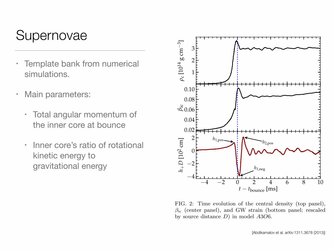
• Template bank from numerical simulations.

• Main parameters:

• Total angular momentum of the inner core at bounce

• Inner core’s ratio of rotational kinetic energy to gravitational energy

5

Model A ⌦c,min

⌦c,max

�ic,b,min

�ic,b,max

Numbersequence [km] [rad s�1] [rad s�1] [10�2] of modelsA1 300 1 15.5 1.62 0.21 30A2 417 1 11.5 3.13 0.19 22A3 634 1 9.5 3.58 0.18 18A4 1268 1 6.5 4.66 0.13 12A5 10000 1 5.5 5.15 0.11 10

TABLE I: Summary of key parameters of our model sequences. ⌦c,max

is the central angular velocity corresponding to thefastest spinning model in each A-sequence. �

ic,b,min

and �ic,b,max

are the values of � = T/|W | of the inner core at bounce forthe slowest and fastest rotators of each sequence, respectively. Note that ⌦

c,max

and �ic,b,max

in the only mildly di↵erentiallyrotating sequence A4 and A5 are limited by the fact that more rapidly spinning models fail to collapse. In more di↵erentiallyrotating models, ⌦

c,max

is the value for which we obtain �ic,b,max

. Due to centrifugal e↵ects, models with higher initial ⌦c

yieldsmaller �

ic,b (see, Fig. 4, and, e.g., [26, 37, 50]).

�4 �2 0 2 4 6 8 10�4

�2

0

2h2,pos

h1,pos

h1,neg

0.02

0.04

0.06

0.08

0.10

1

2

3

t � tbounce [ms]� c

[1014

gcm

�3]

�ic

h +D

[102

cm]

FIG. 2: Time evolution of the central density (top panel),�ic

(center panel), and GW strain (bottom panel; rescaledby source distance D) in model A3O6. The arrows indicatethe first three pronounced generic features of the GW signal,labeled h

1,pos, h1,neg, and h

2,pos. The thin vertical dashedline indicates the time of core bounce defined as the time atwhich the equatorial edge of the inner core reaches an en-tropy of 3 k

B

baryon�1. The dashed red line shows the GWstrain for the same model simulated with 50% higher reso-lution in both the angular and radial direction. There is ex-cellent agreement, which suggests that our fiducial resolutionyields converged results.

IV. RESULTS: DYNAMICS AND WAVEFORMS

The top panel of Fig. 2 depicts the time evolutionof the central density ⇢

c

during the last phase of col-lapse, bounce, and the early postbounce phase of model

FIG. 3: Ratio of rotational kinetic energy to gravitational en-ergy of the inner core at bounce �

ic,b as a function of initialcentral angular velocity ⌦

c

. All model sequences, from nearuniform rotation (A5) to strong di↵erential rotation (A1),are shown. Sequences with uniform or moderate di↵eren-tial rotation terminate at ⌦c beyond which they would befully centrifugally supported already at the onset of collapse.Cf. Table I. Note that the mapping ⌦c ! �

ic,b depends onprogenitor structure [38].

A3O6, which is representative for many of the simulatedmodels. For future reference, we define the time of core

bounce as the moment at which the specific entropy atthe edge of the inner core in the equatorial plane reaches3 k

B

baryon�1. Just before bounce, ⇢c

increases rapidlydue to the accelerated contraction of the inner core. Oncenuclear density is reached, the sti↵ening of the nuclearEOS abruptly decelerates collapse. The inner core over-shoots its equilibrium configuration due to its immenseinertia, and consequently ⇢

c

reaches ⇠3.7 ⇥ 1014 g cm�3

at maximum contraction. The core bounces back and set-tles at a postbounce (pb) quasi-equilibrium central den-sity ⇢

c,pb of ⇠3⇥1014 g cm�3, after a series of ring-downoscillations that last for ⇠10 � 15 ms. These oscillations

[Abdikamalov et al. arXiv:1311.3678 (2013)]

Supernovae

[Edwards et al. arXiv:1407.7549 (2014)]

Bayesian parameter estimation of core collapse supernovae 5

The signals were initially sampled at 100 kHz and subsequently downsampled by

a rational factor to 16384 Hz — the sampling rate of the Advanced LIGO detectors.

Downsampling by a rational factor essentially involved two steps: upsampling by an

integer factor via interpolation and then applying a low-pass filter to eliminate the

high frequency components necessary to avoid aliasing at lower sampling rates; and

downsampling by an integer factor to achieve the desired sampling rate [51]. The

resampled data was zero-bu↵erred to ensure each signal was the same length, N = 16384,

which corresponded to 1 s of data at the Advanced LIGO sampling rate. Each signal

was then aligned so that the first negative peak (not necessarily the global minimum),

corresponding to the time of core bounce, occurred halfway through the time series.

In this analysis, the source of a GW emission is assumed to be optimally oriented

(perpendicular) to a single interferometer. Each signal is linearly polarized with zero

cross-polarization.

−100

0

100h +

D (c

m) A1O4.5

A2O3.5A3O3.0A4O2.5A5O2.5

−250

0

250

0.50 0.51 0.52Time (s)

h +D

(cm

) A1O8.0A2O6.0A3O5.5A4O5.0A5O5.0

Figure 1: A snapshot of the Abdikamalov et al [45] catalogue. The top panel shows the

GW strain (scaled by source distance) for five models with di↵erent levels of precollapse

di↵erential rotation (from strongest di↵erential rotation A1 to weakest A5), each with

�ic,b ⇠ 0.03 (i.e., slowly rotating progenitors). The bottom panel is the same, but for

rapidly rotating progenitors with �ic,b ⇠ 0.09.

We can see a general waveform morphology in figure 1. During core collapse,

there is a slow increase in GW strain until the first local maximum is reached (before

0.5 s). This is followed by core bounce, where the strain rapidly decreases towards a

local minimum (at 0.5 s). This corresponds to the time when the inner core expands

at bounce. After this, there is a period of ring-down oscillations. For slowly rotating

Post-merger neutron star

• Un-modeled, high-frequency search

• Mass-dependent relationship:

!

!

• Peak frequency

• Radius of a fiducial 1.6M⊙

neutron star

• Neutron start Equation of State signature

5

−0.002 0.003 0.008 0.013 0.018

Time [s]

−3

−2

−1

0

1

2

3

h+(t)

×10−20 Target Waveform

1500 2000 2500 3000 3500 4000

Frequency [Hz]

0

1

2

3

4

5

| h2(

f)|[

Hz−

1]

×10−48

0.2

0.4

0.6

0.8

1.0

1.2

1.4

1.6

|hL

1(

f)|2

[Hz−

1]

×10−44 Reconstructions

−0.002 0.008 0.018

Time [s]

−5

0

5

hL

1(t)×

10−

21

0.2

0.4

0.6

0.8

1.0

1.2

1.4

1.6

|hH

1(

f)|2

[Hz−

1]

−0.002 0.008 0.018

Time [s]

−5

0

5

hH

1(t)×

10−

21

1500 2000 2500 3000 3500 4000 4500

Frequency [Hz]

0.0

0.2

0.4

0.6

0.8

1.0

1.2

1.4

|hV

1(

f)|2

[Hz−

1]

−0.002 0.008 0.018

Time [s]

−5

0

5

h V1(t)×

10−

21

1500 2000 2500 3000 3500 4000

Frequency [Hz]

0.00

0.05

0.10

0.15

0.20

0.25

0.30

0.35

|h(

f)|2

[arb

.unit

s]

Average Spectrum and Fits

Average spectrum

NS: BIC =−1880.26

BH: BIC =−1017.21

FIG. 1. Demonstration of signal characterization from the Shen EoS and 1.35–1.35M⊙ system, which results in a survivingPMNS. Left column: the time-series and power spectral density of the ‘plus’ (+) polarisation of the target waveform, for asource located 0.7Mpc from the Earth. A small distance is deliberately chosen to provide a high SNR signal for demonstrativepurposes. Center column: the power spectral densities and time series (insets) of the detector responses reconstructed by theCWB algorithm. The subscripts H1, L1 and V1 refer to simulated results from the LIGO detectors located in Hanford andLivingston, and the Virgo detector, respectively. Right column: the SNR-weighted average reconstructed power spectral densityand fitted models. The model for the delayed collapse scenario is preferred in this instance, as indicated by the relative valuesof the Bayesian Information Criterion (BIC), defined by equation 8, for the delayed and prompt collapse scenarios.

the measurement errors are independent and identicallydistributed according to a normal distribution, the BICis, up to an additive constant which is the same for allmodels:

BIC = n lnχ2min + k lnn, (9)

and

χ2min =

1

n− 1

n!

i=1

(Pi − S∗i )

2, (10)

where Pi and S∗i are the average power spectral density

of the reconstructed detector response and the value ofthe best-fitting model in the ith frequency bin, respec-tively. The best-fit model is found via least-squares min-imisation where the value of the center frequency of theGaussian component f

′

peak is constrained to lie above therelevant value from table I and the power law is con-strained such that α < 0.

Figure 3 shows the workflow of this detection and clas-sification analysis pipeline. The proposed procedure is:

1. We assume a robust detection of an inspiral signalfrom BNS is achieved from a separate analysis, pro-viding an estimate for the time of coalescence andtotal mass of the system.

2. A high-frequency CWB analysis is performed in asmall time window around the time of coalescenceof the BNS inspiral. The CWB analysis is con-strained to [1.5, 4] kHz.

3. If CWB detects statistically significant excesspower in a small time window around the time ofBNS coalescence, assume this is associated with thecoalescence and attempt to classify as follows.

4. Construct PSDs of detector reconstructions, {Pi}jand average according to equation 5 to obtain {Pi}.

[Clark et al. arXiv:1406.5444 (2014)]

fpeak ) R1.6

Bursts

• Gamma-Ray Bursts (see the talk by Michał Wąs)

• Do Intermediate Mass Black Holes exist? (Aasi et al. Phys. Rev. D 89, 122003 (2014))

• Targets:

• Intermediate mass ratio inspirals

• Eccentric binary black holes

• Chirp mass reconstruction

25

Bursts

• Un-modelled searches: the unexpected in gravitational-wave astronomy !

• Flux, amplitude, frequency profile, duration, sky localisation, polarisation, …

26[Abadie et al. Phys. Rev. D 85,122007 (2012)]

8

FIG. 2: Representative waveforms injected into data for simulation studies. The top row is the time domain and the bottomrow is a time-frequency domain representation of the waveform. From left to right: a 361 Hz Q = 9 sine-Gaussian, a ⌧ = 4.0 msGaussian waveform, a white noise burst with a bandwidth of 1000–2000 Hz and characteristic duration of ⌧ = 20 ms and,finally, a ringdown waveform with a frequency of 2000 Hz and ⌧ = 1 ms.

• Band-limited white noise signals:The polarization components are bursts of uncorre-lated band-limited white noise, time shaped with aGaussian profile; H+ andH⇥ have — on average —equal RMS amplitudes and symmetric shape aboutthe central frequency (see Figure 2).

• Neutron star collapse waveforms:For a comparison with previous searches [17, 18],we considered numerical simulations by Baiotti etal. [5], who modeled neutron star gravitational col-lapse to a black hole and the subsequent ring-down.As in previous searches, we chose the models D1 (anearly spherical 1.67 M� neutron star) and D4 (a1.86 M� neutron star that is maximally deformedat the time of its collapse into a black hole) to rep-resent the extremes of the parameter space in massand spin considered in the aforementioned work.Both waveforms are linearly polarized (H⇥ = 0)and their emission is peaked at a few kHz.

The simulated signals were injected with many ampli-tude scale factors to trace out the detection e�ciency asa function of signal strength. The amplitude of the sig-nal is expressed in terms of the root-sum-square strainamplitude (hrss) arriving at the Earth, defined as:

hrss =

sZ|h+(t)|2 + |h⇥(t)|2dt (3.8)

The signal amplitude at a detector is modulated by thedetector antenna pattern functions, expressed as follows:

hdet(t) = F+(⇥,�, )h+(t) + F⇥(⇥,�, )h⇥(t) (3.9)

where F+ and F⇥ are the antenna pattern functions,which depend on the orientation of the wavefront relativeto the detector, denoted here in terms of the sky position

(⇥,�), and on the polarization angle . The sky po-sitions of simulated signals are distributed isotropicallyand polarization angles are chosen to be uniformly dis-tributed. The detection e�ciency is defined as the frac-tion of signals successfully recovered using the same se-lection thresholds and DQFs as in the actual search. Thedetection e�ciency of the search depends on the networkconfiguration and the selection cuts used in the analysis.Detection e�ciencies for the H1L1V1 network for se-

lected waveforms as a function of signal amplitude hrss

and as a function of distance (for the D1 and D4 wave-forms from Baiotti et al. [5]) are reported in Figures 3and 4 , respectively. As in the previous joint run, typicalsensitivities for this network in terms of hrss for the se-lected waveforms lie in the range ⇠ 5⇥ 10�22 Hz�1/2 to⇠ 1 ⇥ 10�20 Hz�1/2; typical distances at 50% detectione�ciency for neutron star collapse waveforms lie in therange ⇠ 50 pc to ⇠ 200 pc.Two convenient characterizations of the sensitivity,

the hrss at 50% and 90% detection e�ciency (h50%rss and

h90%rss respectively) are obtained from fitting the e�ciency

curves and are reported in Tables II, III, and IV for thevarious families. Notice that the 3-fold network, H1L1V1,has a better sensitivity than the weighted average overall networks: 2-fold networks have ⇠ 3/4 of the analyzedlive time, but feature a lower sensitivity.

D. Systematic Uncertainties

The most relevant systematic uncertainty in the astro-physical interpretation of our results is due to the cal-ibration error on the strain data produced by each de-tector [34, 35]. The e↵ect of calibration systematics onnetwork detection e�ciency has been estimated by dedi-cated simulations of GW signals in which the signal am-plitude and phase at each detector is randomly jittered